Ch19 mish11 embfm

Chapter 19Quantity Theory, Inflation and the

Demand for Money

© 2016 Pearson Education, Inc. All rights reserved. 19-2

Preview

• This chapter examines the quantity theory of money and its link to the demand for money

• The link between interest rates and the demand for money is then addressed


Learning Objectives

• Assess the relationship between money growth and inflation in the short run and the long run, as implied by the quantity theory of money.

• Identify the circumstances under which budget deficits can lead to inflationary monetary policy.

• Summarize the three motives underlying the liquidity preference theory of money demand.


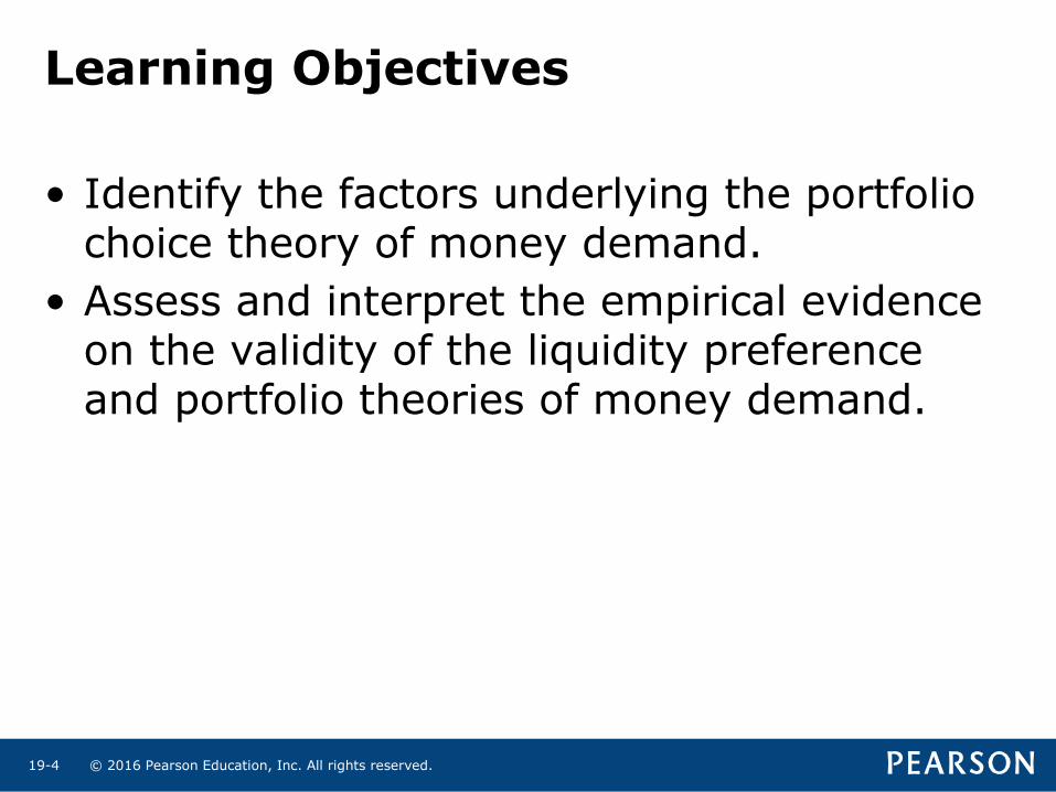
Learning Objectives

• Identify the factors underlying the portfolio choice theory of money demand.

• Assess and interpret the empirical evidence on the validity of the liquidity preference and portfolio theories of money demand.


Quantity Theory of Money

M = the money supply

P = price level

Y = aggregate output (income)

P × Y = aggregate nominal income (nominal GDP)

V = velocity of money (average number of times per year that a dollar is spent)

V = P × Y

MEquation of Exchange

M ×V = P × Y

Velocity of Money and The Equation of Exchange:


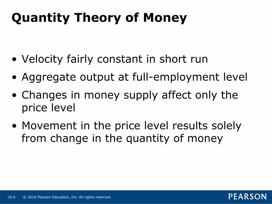
• Velocity fairly constant in short run

• Aggregate output at full-employment level

• Changes in money supply affect only the price level

• Movement in the price level results solely from change in the quantity of money



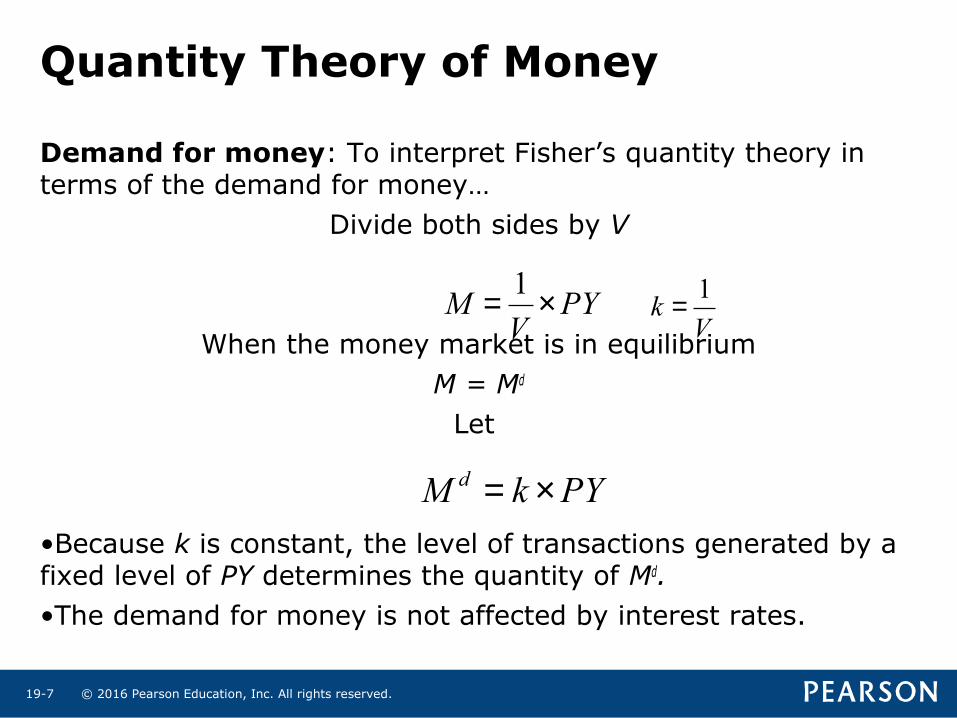
Demand for money: To interpret Fisher’s quantity theory in terms of the demand for money…

Divide both sides by V

When the money market is in equilibriumM = Md

Let

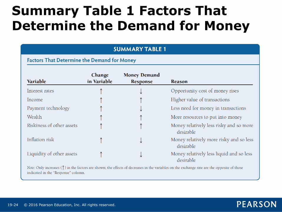
•Because k is constant, the level of transactions generated by a fixed level of PY determines the quantity of Md.•The demand for money is not affected by interest rates.

PYV

M ×= 1V

k1=

PYkM d ×=



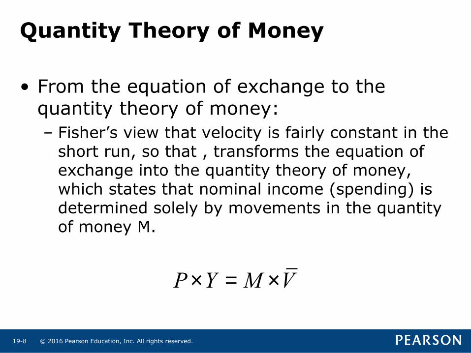
• From the equation of exchange to the quantity theory of money:– Fisher’s view that velocity is fairly constant in the

short run, so that , transforms the equation of exchange into the quantity theory of money, which states that nominal income (spending) is determined solely by movements in the quantity of money M.

P Y M V× = ×



Quantity Theory and the Price Level

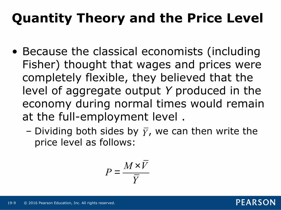
• Because the classical economists (including Fisher) thought that wages and prices were completely flexible, they believed that the level of aggregate output Y produced in the economy during normal times would remain at the full-employment level .– Dividing both sides by , we can then write the

price level as follows:

M VP

Y

×=

Y


Quantity Theory and Inflation

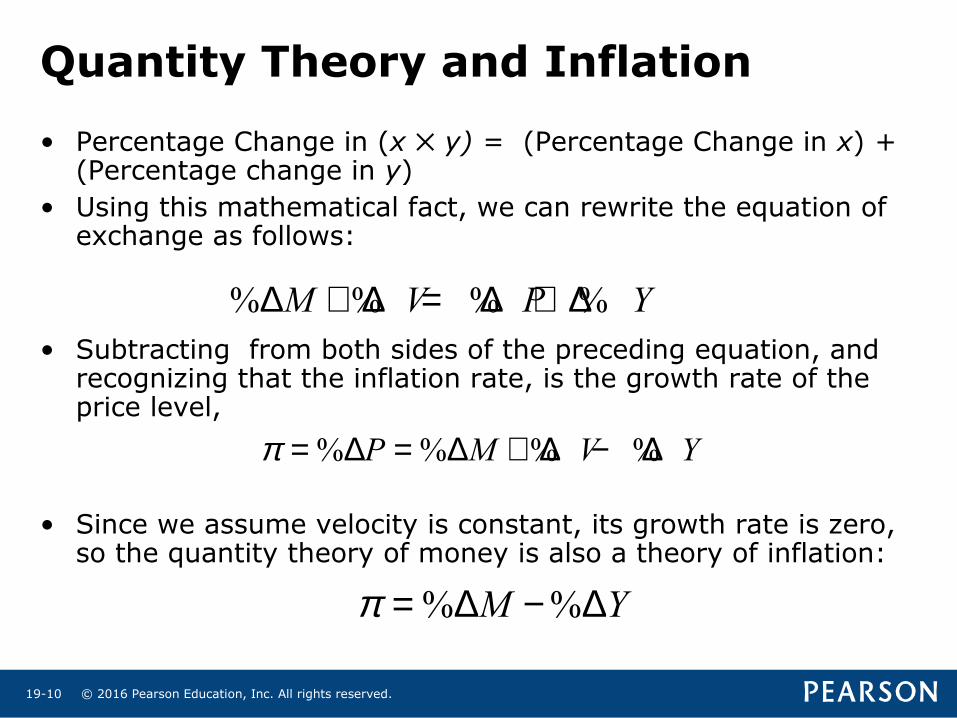
• Percentage Change in (x ✕ y) = (Percentage Change in x) + (Percentage change in y)

• Using this mathematical fact, we can rewrite the equation of exchange as follows:

• Subtracting from both sides of the preceding equation, and recognizing that the inflation rate, is the growth rate of the price level,

• Since we assume velocity is constant, its growth rate is zero, so the quantity theory of money is also a theory of inflation:

% % % %M V P Y∆ + ∆ = ∆ + ∆

% % % %P M V Yπ = ∆ = ∆ + ∆ − ∆

% %M Yπ = ∆ − ∆


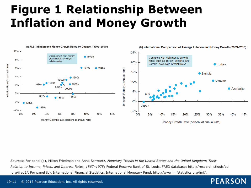
Figure 1 Relationship Between Inflation and Money Growth

Sources: For panel (a), Milton Friedman and Anna Schwartz, Monetary Trends in the United States and the United Kingdom: Their

Relation to Income, Prices, and Interest Rates, 1867–1975; Federal Reserve Bank of St. Louis, FRED database: http://research.stlouisfed

.org/fred2/. For panel (b), International Financial Statistics. International Monetary Fund, http://www.imfstatistics.org/imf/.


Figure 2 Annual U.S. Inflation and Money Growth Rates, 1965–2015

Sources: Federal Reserve Bank of St. Louis, FRED database: http://research.stlouisfed.org/fred2/.


Budget Deficits and Inflation

• There are two ways the government can pay for spending: raise revenue or borrow– Raise revenue by levying taxes or go into debt by

issuing government bonds

• The government can also create money and use it to pay for the goods and services it buys


• The government budget constraint thus reveals two important facts:– If the government deficit is financed by an

increase in bond holdings by the public, there is no effect on the monetary base and hence on the money supply.

– But, if the deficit is not financed by increased bond holdings by the public, the monetary base and the money supply increase.

Budget Deficits and Inflation


Hyperinflation

• Hyperinflations are periods of extremely high inflation of more than 50% per month.

• Many economies—both poor and developed—have experienced hyperinflation over the last century, but the United States has been spared such turmoil.

• One of the most extreme examples of hyperinflation throughout world history occurred recently in Zimbabwe in the 2000s.


Keynesian Theories of Money Demand

• Keynes’s liquidity preference theory

• Why do individuals hold money? Three motives:– Transactions motive

– Precautionary motive

– Speculative motive

• Distinguishes between real and nominal quantities of money


Transactions Motive

• Keynes initially accepted the quantity theory view that the transactions component is proportional to income.

• Later, he and other economists recognized that new methods for payment, referred to as payment technology, could also affect the demand for money.


Precautionary Motive

• Keynes also recognized that people hold money as a cushion against unexpected wants.

• Keynes argued that the precautionary money balances people want to hold would also be proportional to income.


Speculative Motive

• Keynes also believed people choose to hold money as a store of wealth, which he called the speculative motive.


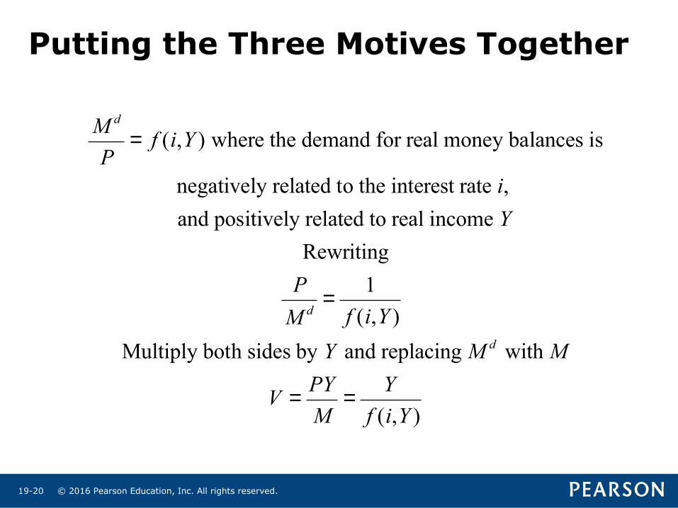
M d

P= f (i,Y ) where the demand for real money balances is

negatively related to the interest rate i,

and positively related to real income Y

Rewriting

P

M d= 1

f (i,Y )

Multiply both sides by Y and replacing M d with M

V = PY

M= Y

f (i,Y )

Putting the Three Motives Together


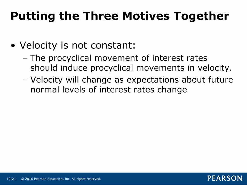
Putting the Three Motives Together

• Velocity is not constant:– The procyclical movement of interest rates

should induce procyclical movements in velocity.– Velocity will change as expectations about future

normal levels of interest rates change


Portfolio Theories of Money Demand

• Theory of portfolio choice and Keynesian liquidity preference – The theory of portfolio choice can justify the

conclusion from the Keynesian liquidity preference function that the demand for real money balances is positively related to income and negatively related to the nominal interest rate.


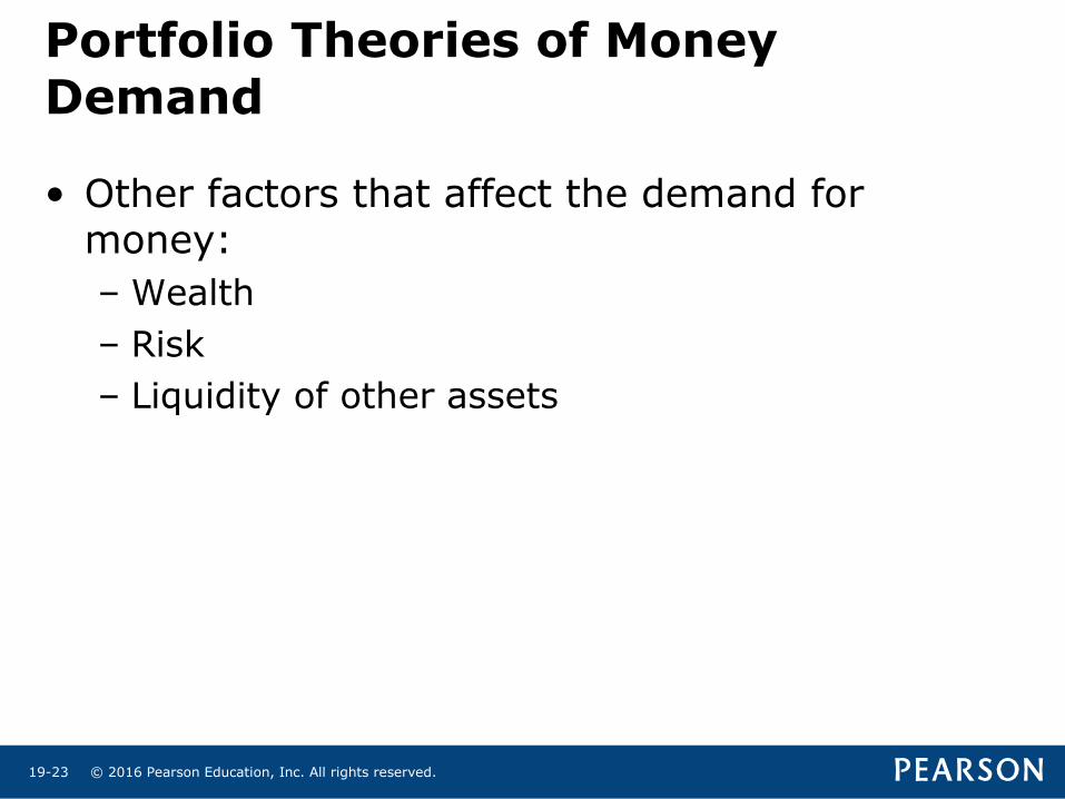
• Other factors that affect the demand for money:– Wealth– Risk– Liquidity of other assets

Portfolio Theories of Money Demand


Summary Table 1 Factors That Determine the Demand for Money


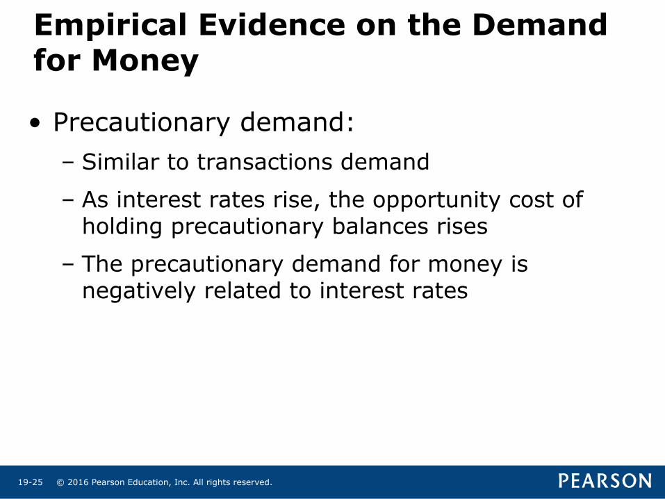
• Precautionary demand:– Similar to transactions demand

– As interest rates rise, the opportunity cost of holding precautionary balances rises

– The precautionary demand for money is negatively related to interest rates

Empirical Evidence on the Demand for Money


Interest Rates and Money Demand

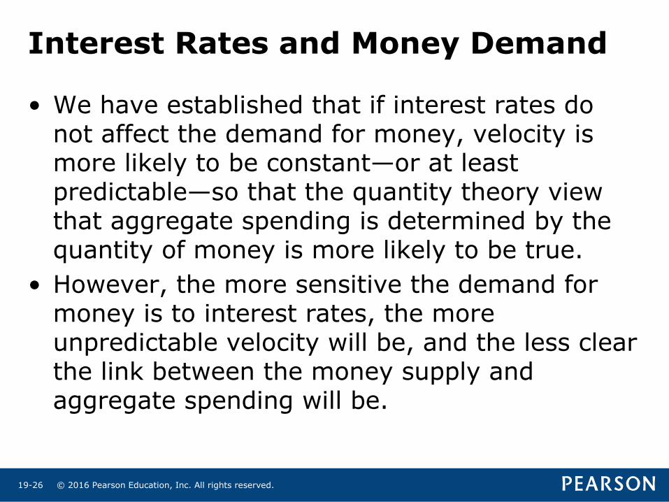
• We have established that if interest rates do not affect the demand for money, velocity is more likely to be constant—or at least predictable—so that the quantity theory view that aggregate spending is determined by the quantity of money is more likely to be true.

• However, the more sensitive the demand for money is to interest rates, the more unpredictable velocity will be, and the less clear the link between the money supply and aggregate spending will be.


Stability of Money Demand

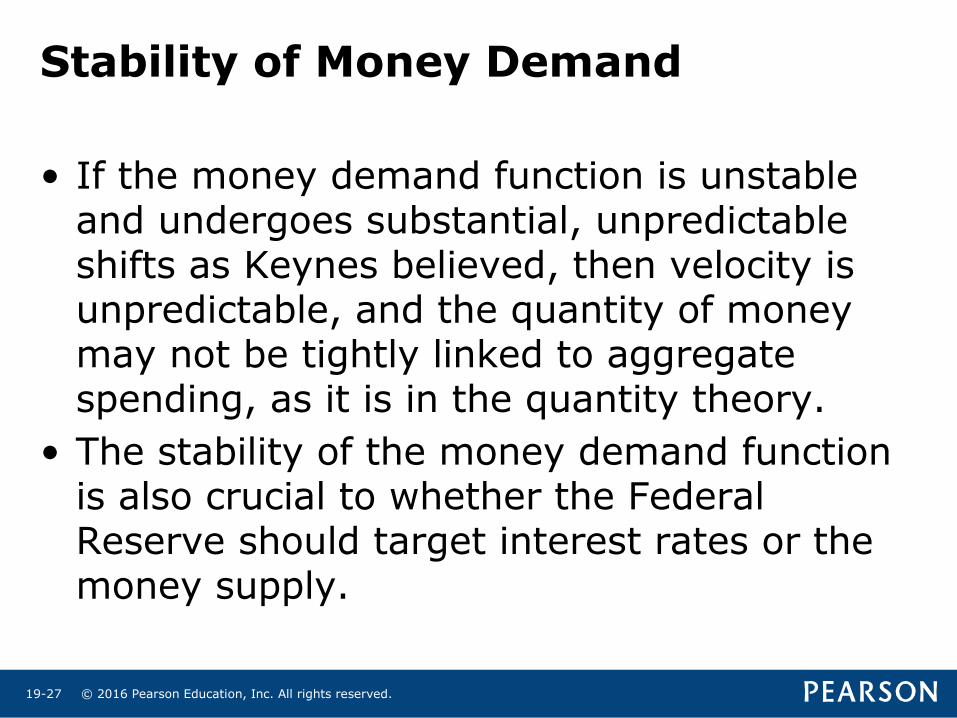
• If the money demand function is unstable and undergoes substantial, unpredictable shifts as Keynes believed, then velocity is unpredictable, and the quantity of money may not be tightly linked to aggregate spending, as it is in the quantity theory.

• The stability of the money demand function is also crucial to whether the Federal Reserve should target interest rates or the money supply.


Stability of Money Demand

• If the money demand function is unstable and so the money supply is not closely linked to aggregate spending, then the level of interest rates the Fed sets will provide more information about the stance of monetary policy than will the money supply.

Documents

Ch19 mish11 embfm