Spring 1, 2013

Chapter 4. Ch 04 P35 Build a ModelExcept for charts and answers that must be written, only Excel formulas that use cell references or functions will be accepted for credit. Numeric answers in cells will not be accepted.

Inputs: PV = 1000I/YR = 10%N = 5

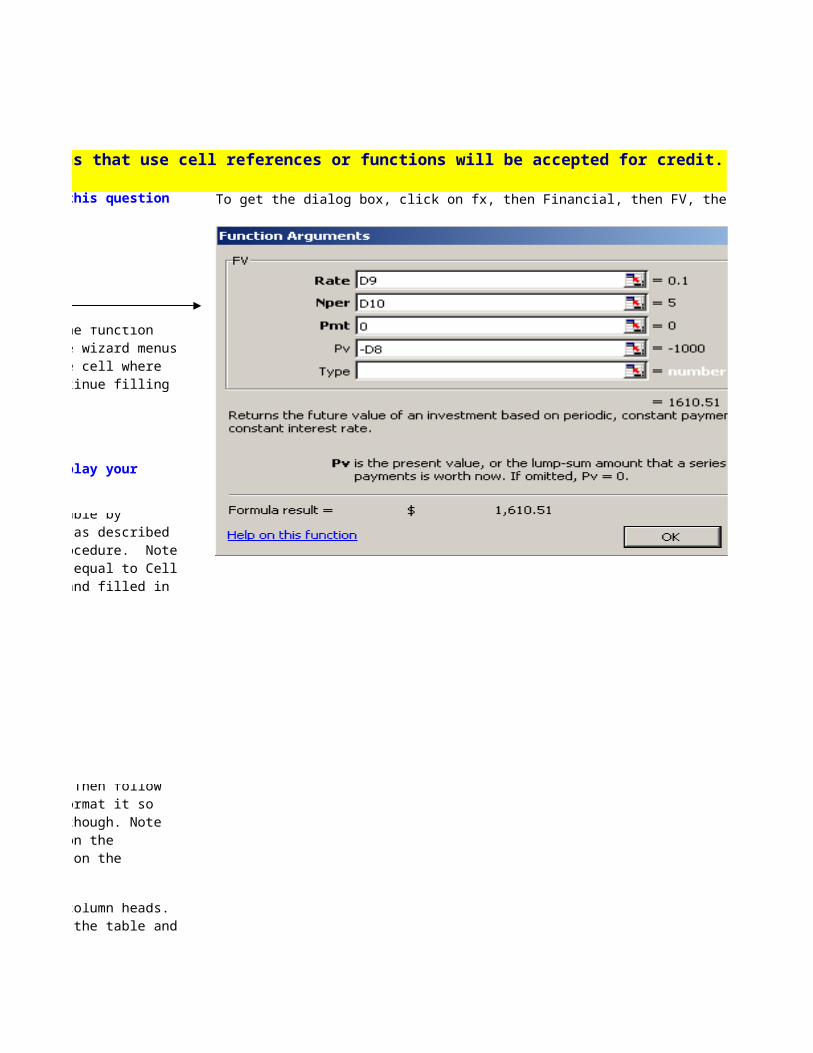
Formula: FV = PV(1+I)^N = $ 1,610.51 Wizard (FV): $1,610.51

Experiment by changing the input values to see how quickly the output values change.

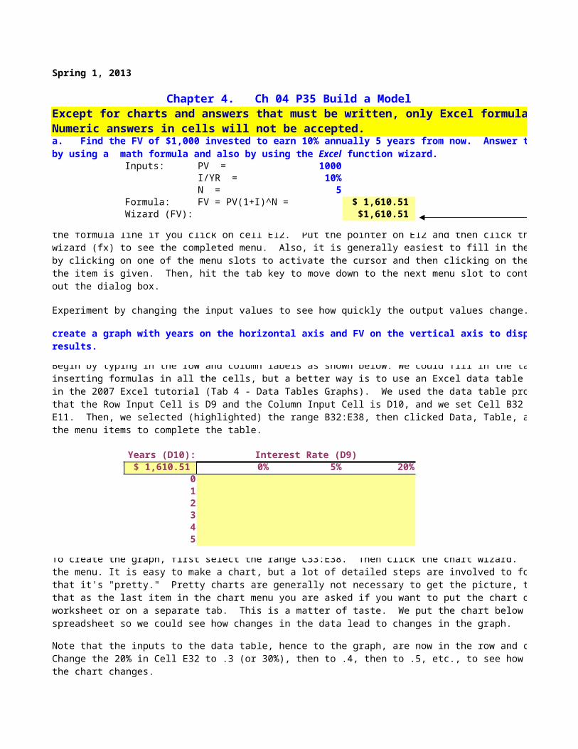
Years (D10): Interest Rate (D9) $ 1,610.51 0% 5% 20%

012345

a. Find the FV of $1,000 invested to earn 10% annually 5 years from now. Answer this question by using a math formula and also by using the Excel function wizard.

Note: When you use the wizard and fill in the menu items, the result is the formula you see on the formula line if you click on cell E12. Put the pointer on E12 and then click the function wizard (fx) to see the completed menu. Also, it is generally easiest to fill in the wizard menus by clicking on one of the menu slots to activate the cursor and then clicking on the cell where the item is given. Then, hit the tab key to move down to the next menu slot to continue filling out the dialog box.

b. Now create a table that shows the FV at 0%, 5%, and 20% for 0, 1, 2, 3, 4, and 5 years. Then create a graph with years on the horizontal axis and FV on the vertical axis to display your results.

Begin by typing in the row and column labels as shown below. We could fill in the table by inserting formulas in all the cells, but a better way is to use an Excel data table as described in the 2007 Excel tutorial (Tab 4 - Data Tables Graphs). We used the data table procedure. Note that the Row Input Cell is D9 and the Column Input Cell is D10, and we set Cell B32 equal to Cell E11. Then, we selected (highlighted) the range B32:E38, then clicked Data, Table, and filled in the menu items to complete the table.

To create the graph, first select the range C33:E38. Then click the chart wizard. Then follow the menu. It is easy to make a chart, but a lot of detailed steps are involved to format it so that it's "pretty." Pretty charts are generally not necessary to get the picture, though. Note that as the last item in the chart menu you are asked if you want to put the chart on the worksheet or on a separate tab. This is a matter of taste. We put the chart below on the spreadsheet so we could see how changes in the data lead to changes in the graph.

Note that the inputs to the data table, hence to the graph, are now in the row and column heads. Change the 20% in Cell E32 to .3 (or 30%), then to .4, then to .5, etc., to see how the table and the chart changes.

Inputs: FV = 1000I/YR = 10%N = 5

Formula: PV = FV/(1+I)^N = $ 620.92 Wizard (PV): $ 620.92

d. A security has a cost of $1,000 and will return $2,000 after 5 years. What rate of return does the security provide?

Inputs: PV = -1000FV = 2000I/YR = ?N = 5

Wizard (Rate): 14.87%

Inputs: PV = -30FV = 60I/YR = growth rate 2%N = ?

Wizard (NPER): 35.00 = Years to double.

c. Find the PV of $1,000 due in 5 years if the discount rate is 10% per year. Again, work the problem with a formula and also by using the function wizard.

Note: In the wizard's menu, use zero for Pmt because there are no periodic payments. Also, set the FV with a negative sign so that the PV will appear as a positive number.

Note: Use zero for Pmt since there are no periodic payments. Note that the PV is given a negative sign because it is an outflow (cost to buy the security). Also, note that you must scroll down the menu to complete the inputs.

e. Suppose California’s population is 30 million people, and its population is expected to grow by 2% per year. How long would it take for the population to double?

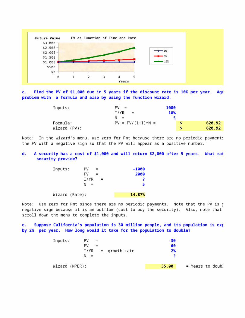
0 1 2 3 4 5

$0

$500

$1,000

$1,500

$2,000

$2,500

$3,000

FV as Function of Time and Rate

0%

5%

10%

Years

Future Value

Inputs: PMT = $ 1,000 N = 5 I/YR = 15%

PV: Use function wizard (PV) PV = -$3,352.16

FV: Use function wizard (FV) FV = -$6,742.38

g. How would the PV and FV of the above annuity change if it were an annuity due rather than an ordinary annuity?

PV annuity due = -$3,352.16 x 115% = -$3,854.98

Exactly the same adjustment is made to find the FV of the annuity due.

FV annuity due = -$6,742.38 x 115% = -$7,753.74

h. What would the FV and the PV for parts a and c be if the interest rate were 10% with

Part a. FV with semiannual compounding: Orig. Inputs New InputsInputs: PV = 1000 1000

I/YR = 10% 5%N = 5 10

Formula: FV = PV(1+I)^N = $ 1,610.51 $ 1,628.89 Wizard (FV): $ 1,610.51 $ 1,628.89

Part c. PV with semiannual compounding: Orig. Inputs New InputsInputs: FV = 1000 1000

I/YR = 10% 5%N = 5 10

Formula: PV = FV/(1+I)^N = $ 620.92 $ 613.91 Wizard (PV): $ 620.92 $ 613.91

f. Find the PV of an ordinary annuity that pays $1,000 at the end of each of the next 5 years if the interest rate is 15%. Then find the FV of that same annuity.

For the PV, each payment would be received one period sooner, hence would be discounted back one less year. This would make the PV larger. We can find the PV of the annuity due by finding the PV of an ordinary annuity and then multiplying it by (1 + I).

semiannual compounding rather than 10% with annual compounding?

i. Find the PV and FV of an investment that makes the following end-of-year payments. The interest rate is 8%.

Year Payment1 1002 2003 400

Rate = 8%

To find the PV, use the NPV function: PV = $ 581.59

Year Payment x (1 + I )^(N-t) = FV1 100 1.17 116.64 2 200 1.08 216.00 3 400 1.00 400.00

Sum = $ 732.64

An alternative procedure for finding the FV would be to find the PV of the series using the NPVfunction, then compound that amount, as is done below:

PV = $ 581.59 FV of PV = $ 732.64

Original amount of mortgage: 50000Term of mortgage: 10Interest rate: 0.085

Annual payment (use PMT function): -$7,620.39

Excel does not have a function for the sum of the future values for a set of uneven payments. Therefore, we must find this FV by some other method. Probably the easiest procedure is to simply compound each payment, then sum them, as is done below. Note that since the payments are received at the end of each year, the first payment is compounded for 2 years, the second for 1 year, and the third for 0 years.

j. Suppose you bought a house and took out a mortgage for $50,000. The interest rate is 8.5%, and you must amortize the loan over 10 years with equal end-of-year payments. Set up an amortization schedule that shows the annual payments and the amount of each payment that repays the principal and the amount that constitutes interest expense to the borrower and interest income to the lender.

Year Beg. Amt. Pmt Interest Principal End. Bal.1 $50,000.00 $7,620.39 $4,250.00 $3,370.39 $46,629.612 $46,629.61 $7,620.39 $3,963.52 $3,656.87 $42,972.753 $42,972.75 $7,620.39 $3,652.68 $3,967.70 $39,005.044 $39,005.04 $7,620.39 $3,315.43 $4,304.96 $34,700.095 $34,700.09 $7,620.39 $2,949.51 $4,670.88 $30,029.216 $30,029.21 $7,620.39 $2,552.48 $5,067.90 $24,961.317 $24,961.31 $7,620.39 $2,121.71 $5,498.67 $19,462.638 $19,462.63 $7,620.39 $1,654.32 $5,966.06 $13,496.579 $13,496.57 $7,620.39 $1,147.21 $6,473.18 $7,023.40

10 $7,023.40 $7,620.39 $596.99 $7,023.40 $0.00

(1) Create a graph that shows how the payments are divided between interest and principal repayment over time.

(2) Suppose the loan called for 10 years of monthly payments, 120 payments in all, with the same original amount and the same nominal interest rate. What would the amortization schedule show now?

The monthly payment would be: -$619.93

Go back to cells D184 and D185, and change the interest rate and the term to maturity to see how the payments would change.

Now we would have a 12 × 10 = 120-payment loan at a monthly rate of .085/12 = 0.007083333%.

1 2 3 4 5 6 7 8 9 10$0.00

$1,000.00$2,000.00$3,000.00$4,000.00$5,000.00$6,000.00$7,000.00$8,000.00

Breakdown of Payments

Principal

Interest

Years

Month Beg. Amt. Pmt Interest Principal End. Bal.1 $50,000.00 $619.93 $354.17 $265.76 $49,734.242 $49,734.24 $619.93 $352.28 $267.64 $49,466.593 $49,466.59 $619.93 $350.39 $269.54 $49,197.054 $49,197.05 $619.93 $348.48 $271.45 $48,925.605 $48,925.60 $619.93 $346.56 $273.37 $48,652.236 $48,652.23 $619.93 $344.62 $275.31 $48,376.927 $48,376.92 $619.93 $342.67 $277.26 $48,099.678 $48,099.67 $619.93 $340.71 $279.22 $47,820.449 $47,820.44 $619.93 $338.73 $281.20 $47,539.24

10 $47,539.24 $619.93 $336.74 $283.19 $47,256.0511 $47,256.05 $619.93 $334.73 $285.20 $46,970.8512 $46,970.85 $619.93 $332.71 $287.22 $46,683.6313 $46,683.63 $619.93 $330.68 $289.25 $46,394.3814 $46,394.38 $619.93 $328.63 $291.30 $46,103.0815 $46,103.08 $619.93 $326.56 $293.36 $45,809.7116 $45,809.71 $619.93 $324.49 $295.44 $45,514.2717 $45,514.27 $619.93 $322.39 $297.54 $45,216.7418 $45,216.74 $619.93 $320.29 $299.64 $44,917.0919 $44,917.09 $619.93 $318.16 $301.77 $44,615.3320 $44,615.33 $619.93 $316.03 $303.90 $44,311.4221 $44,311.42 $619.93 $313.87 $306.06 $44,005.3722 $44,005.37 $619.93 $311.70 $308.22 $43,697.1423 $43,697.14 $619.93 $309.52 $310.41 $43,386.7424 $43,386.74 $619.93 $307.32 $312.61 $43,074.1325 $43,074.13 $619.93 $305.11 $314.82 $42,759.3126 $42,759.31 $619.93 $302.88 $317.05 $42,442.2627 $42,442.26 $619.93 $300.63 $319.30 $42,122.9728 $42,122.97 $619.93 $298.37 $321.56 $41,801.4129 $41,801.41 $619.93 $296.09 $323.84 $41,477.5730 $41,477.57 $619.93 $293.80 $326.13 $41,151.4431 $41,151.44 $619.93 $291.49 $328.44 $40,823.0132 $40,823.01 $619.93 $289.16 $330.77 $40,492.2433 $40,492.24 $619.93 $286.82 $333.11 $40,159.1334 $40,159.13 $619.93 $284.46 $335.47 $39,823.6635 $39,823.66 $619.93 $282.08 $337.84 $39,485.8236 $39,485.82 $619.93 $279.69 $340.24 $39,145.5837 $39,145.58 $619.93 $277.28 $342.65 $38,802.9438 $38,802.94 $619.93 $274.85 $345.07 $38,457.8639 $38,457.86 $619.93 $272.41 $347.52 $38,110.3440 $38,110.34 $619.93 $269.95 $349.98 $37,760.3641 $37,760.36 $619.93 $267.47 $352.46 $37,407.9042 $37,407.90 $619.93 $264.97 $354.96 $37,052.9543 $37,052.95 $619.93 $262.46 $357.47 $36,695.4844 $36,695.48 $619.93 $259.93 $360.00 $36,335.4745 $36,335.47 $619.93 $257.38 $362.55 $35,972.9246 $35,972.92 $619.93 $254.81 $365.12 $35,607.8047 $35,607.80 $619.93 $252.22 $367.71 $35,240.1048 $35,240.10 $619.93 $249.62 $370.31 $34,869.7849 $34,869.78 $619.93 $246.99 $372.93 $34,496.85

50 $34,496.85 $619.93 $244.35 $375.58 $34,121.2751 $34,121.27 $619.93 $241.69 $378.24 $33,743.0452 $33,743.04 $619.93 $239.01 $380.92 $33,362.1253 $33,362.12 $619.93 $236.32 $383.61 $32,978.5154 $32,978.51 $619.93 $233.60 $386.33 $32,592.1855 $32,592.18 $619.93 $230.86 $389.07 $32,203.1156 $32,203.11 $619.93 $228.11 $391.82 $31,811.2957 $31,811.29 $619.93 $225.33 $394.60 $31,416.6958 $31,416.69 $619.93 $222.53 $397.39 $31,019.3059 $31,019.30 $619.93 $219.72 $400.21 $30,619.0960 $30,619.09 $619.93 $216.89 $403.04 $30,216.0561 $30,216.05 $619.93 $214.03 $405.90 $29,810.1562 $29,810.15 $619.93 $211.16 $408.77 $29,401.3763 $29,401.37 $619.93 $208.26 $411.67 $28,989.7164 $28,989.71 $619.93 $205.34 $414.58 $28,575.1265 $28,575.12 $619.93 $202.41 $417.52 $28,157.6066 $28,157.60 $619.93 $199.45 $420.48 $27,737.1267 $27,737.12 $619.93 $196.47 $423.46 $27,313.6668 $27,313.66 $619.93 $193.47 $426.46 $26,887.2169 $26,887.21 $619.93 $190.45 $429.48 $26,457.7370 $26,457.73 $619.93 $187.41 $432.52 $26,025.2171 $26,025.21 $619.93 $184.35 $435.58 $25,589.6372 $25,589.63 $619.93 $181.26 $438.67 $25,150.9673 $25,150.96 $619.93 $178.15 $441.78 $24,709.1874 $24,709.18 $619.93 $175.02 $444.91 $24,264.2875 $24,264.28 $619.93 $171.87 $448.06 $23,816.2276 $23,816.22 $619.93 $168.70 $451.23 $23,364.9977 $23,364.99 $619.93 $165.50 $454.43 $22,910.5678 $22,910.56 $619.93 $162.28 $457.65 $22,452.9279 $22,452.92 $619.93 $159.04 $460.89 $21,992.0380 $21,992.03 $619.93 $155.78 $464.15 $21,527.8881 $21,527.88 $619.93 $152.49 $467.44 $21,060.4482 $21,060.44 $619.93 $149.18 $470.75 $20,589.6983 $20,589.69 $619.93 $145.84 $474.08 $20,115.6184 $20,115.61 $619.93 $142.49 $477.44 $19,638.1685 $19,638.16 $619.93 $139.10 $480.82 $19,157.3486 $19,157.34 $619.93 $135.70 $484.23 $18,673.1187 $18,673.11 $619.93 $132.27 $487.66 $18,185.4588 $18,185.45 $619.93 $128.81 $491.11 $17,694.3389 $17,694.33 $619.93 $125.33 $494.59 $17,199.7490 $17,199.74 $619.93 $121.83 $498.10 $16,701.6491 $16,701.64 $619.93 $118.30 $501.63 $16,200.0292 $16,200.02 $619.93 $114.75 $505.18 $15,694.8493 $15,694.84 $619.93 $111.17 $508.76 $15,186.0894 $15,186.08 $619.93 $107.57 $512.36 $14,673.7295 $14,673.72 $619.93 $103.94 $515.99 $14,157.7396 $14,157.73 $619.93 $100.28 $519.64 $13,638.0997 $13,638.09 $619.93 $96.60 $523.33 $13,114.7698 $13,114.76 $619.93 $92.90 $527.03 $12,587.7399 $12,587.73 $619.93 $89.16 $530.77 $12,056.96

100 $12,056.96 $619.93 $85.40 $534.52 $11,522.44101 $11,522.44 $619.93 $81.62 $538.31 $10,984.13102 $10,984.13 $619.93 $77.80 $542.12 $10,442.00103 $10,442.00 $619.93 $73.96 $545.96 $9,896.04104 $9,896.04 $619.93 $70.10 $549.83 $9,346.21105 $9,346.21 $619.93 $66.20 $553.73 $8,792.48106 $8,792.48 $619.93 $62.28 $557.65 $8,234.83107 $8,234.83 $619.93 $58.33 $561.60 $7,673.24108 $7,673.24 $619.93 $54.35 $565.58 $7,107.66109 $7,107.66 $619.93 $50.35 $569.58 $6,538.08110 $6,538.08 $619.93 $46.31 $573.62 $5,964.46111 $5,964.46 $619.93 $42.25 $577.68 $5,386.78112 $5,386.78 $619.93 $38.16 $581.77 $4,805.01113 $4,805.01 $619.93 $34.04 $585.89 $4,219.11114 $4,219.11 $619.93 $29.89 $590.04 $3,629.07115 $3,629.07 $619.93 $25.71 $594.22 $3,034.85116 $3,034.85 $619.93 $21.50 $598.43 $2,436.42117 $2,436.42 $619.93 $17.26 $602.67 $1,833.75118 $1,833.75 $619.93 $12.99 $606.94 $1,226.81119 $1,226.81 $619.93 $8.69 $611.24 $615.57120 $615.57 $619.93 $4.36 $615.57 $0.00

Except for charts and answers that must be written, only Excel formulas that use cell references or functions will be accepted for credit.

To get the dialog box, click on fx, then Financial, then FV, then OK.

7/22/2012