Embed Size (px)
DESCRIPTION
Ch 7 Decision theory Learning objectives: After completing this chapter, you should be able to: 1.Outline the characteristics of a decision theory approach to decision making. 2.Describe and give examples of decisions under certainty, risk, and complete uncertainty. - PowerPoint PPT Presentation
Citation preview
Ch 7Decision theory
Learning objectives:
After completing this chapter, you should be able to:1.Outline the characteristics of a decision theory approach to decision
making.
2.Describe and give examples of decisions under certainty, risk, and complete uncertainty.
3.Cons tract a payoff table.
4.Use decision trees to lay out decision alternatives and possible consequences of decisions.
SummaryDecision theory is a general approach to decision making. It is very
useful for a decision maker who must choose from a list of a alternative. Knowing that one of a number of possible future states of nature will occur and that this will have an impact on the payoff
realized by a particular alternative.
Glossary
Payoff: a table that shows the payoff for each alternative for each state of nature.
Risk: A decision problem in which the state of nature have probability associated which their occurrence.
Uncertainty: Refers to a decision problem in which probabilities of occurrence for the various states of nature one unknown.
Decision tree: A schematic representation of a decision problem that involves the use of branches and nodes.
Ch.7
Decision theory
1 .Decision making
A. Under certainty .
B. Under complete uncertainty.
C. Under risk.
2 .Decision tree
A. Expected monetary value model.
B. Expected net present value model.
Decision theory
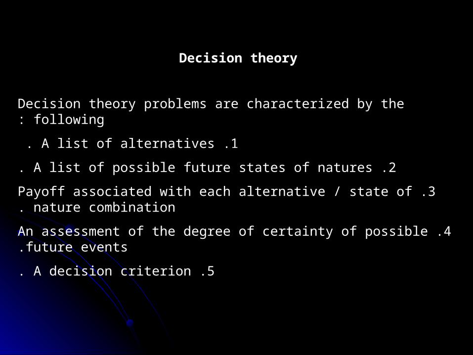
Decision theory problems are characterized by the following:
1 .A list of alternatives .
2 .A list of possible future states of natures.
3 .Payoff associated with each alternative / state of nature combination.
4 .An assessment of the degree of certainty of possible future events.
5 .A decision criterion.
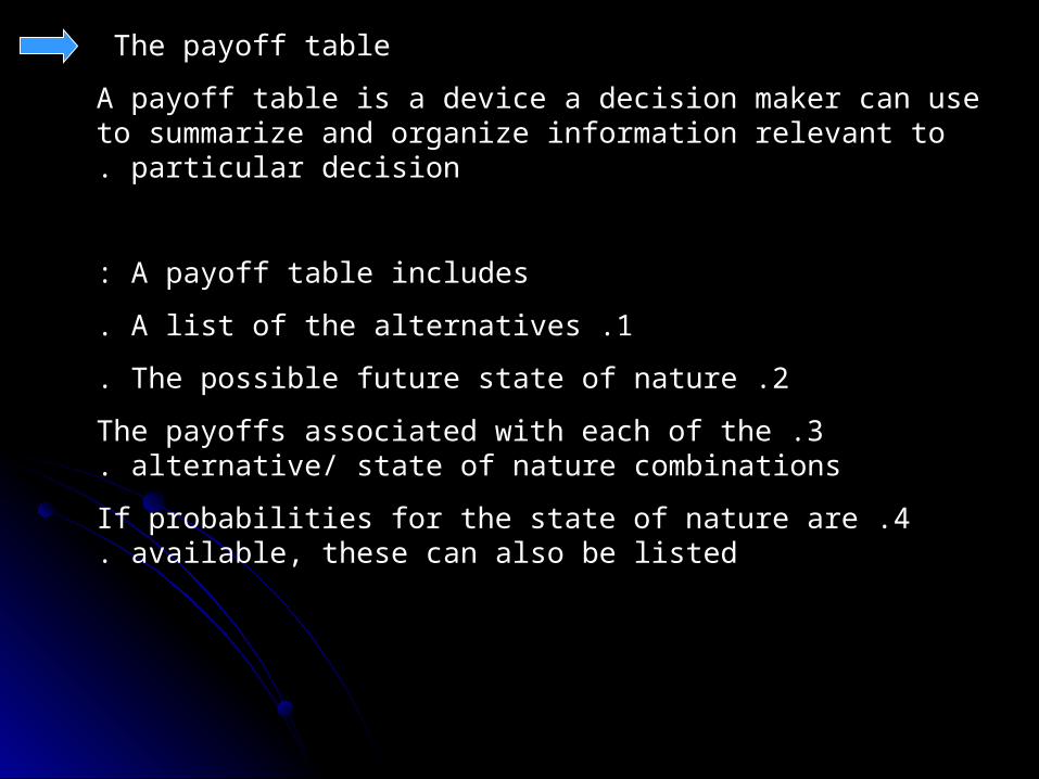
The payoff table
A payoff table is a device a decision maker can use to summarize and organize information relevant to particular decision.
A payoff table includes:
1 .A list of the alternatives.
2 .The possible future state of nature.
3 .The payoffs associated with each of the alternative/ state of nature combinations.
4 .If probabilities for the state of nature are available, these can also be listed.
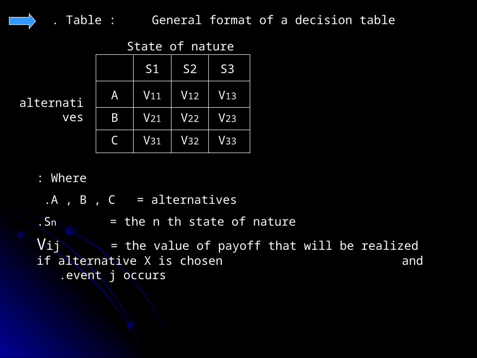
Table : General format of a decision table.
State of nature
alternativesV11 V12 V13
V21 V22 V23
V31 V32 V33
A
B
C
S1 S2 S3
Where:
A , B , C = alternatives .
Sn = the n th state of nature.
Vij = the value of payoff that will be realized if alternative X is chosen and event j occurs.
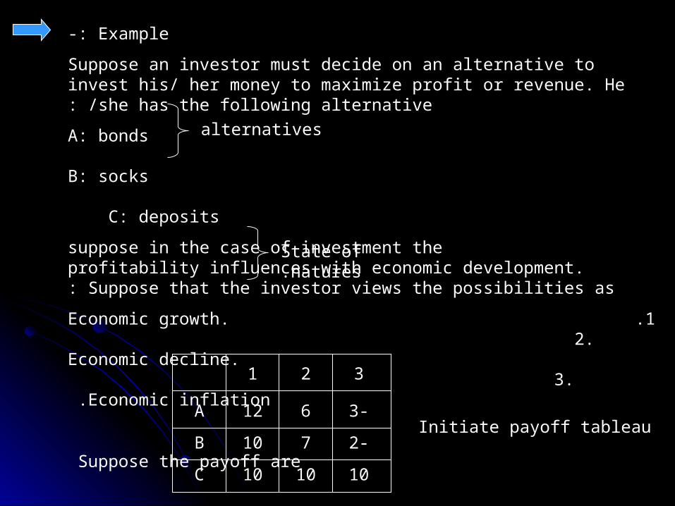
Example-:
Suppose an investor must decide on an alternative to invest his/ her money to maximize profit or revenue. He /she has the following alternative:
A: bonds B: socks
C: deposits
suppose in the case of investment the profitability influences with economic development. Suppose that the investor views the possibilities as:
1 .Economic growth. 2. Economic decline.
3. Economic inflation .
Suppose the payoff are
alternatives
State of natures.
12 6 -3
10 7 -2
10 10 10
A
B
C
1 2 3
Initiate payoff tableau
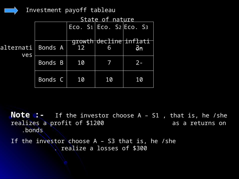
Investment payoff tableau
State of nature
alternatives
Eco. S1 growth
Eco. S2 decline
Eco. S3 inflation
Bonds A
Bonds B
Bonds C
12
10
10
6
7
10
-3
-2
10
Note :- If the investor choose A – S1 , that is, he /she realizes a profit of $1200 as a returns on bonds .
If the investor choose A – S3 that is, he /she realize a losses of $300 .
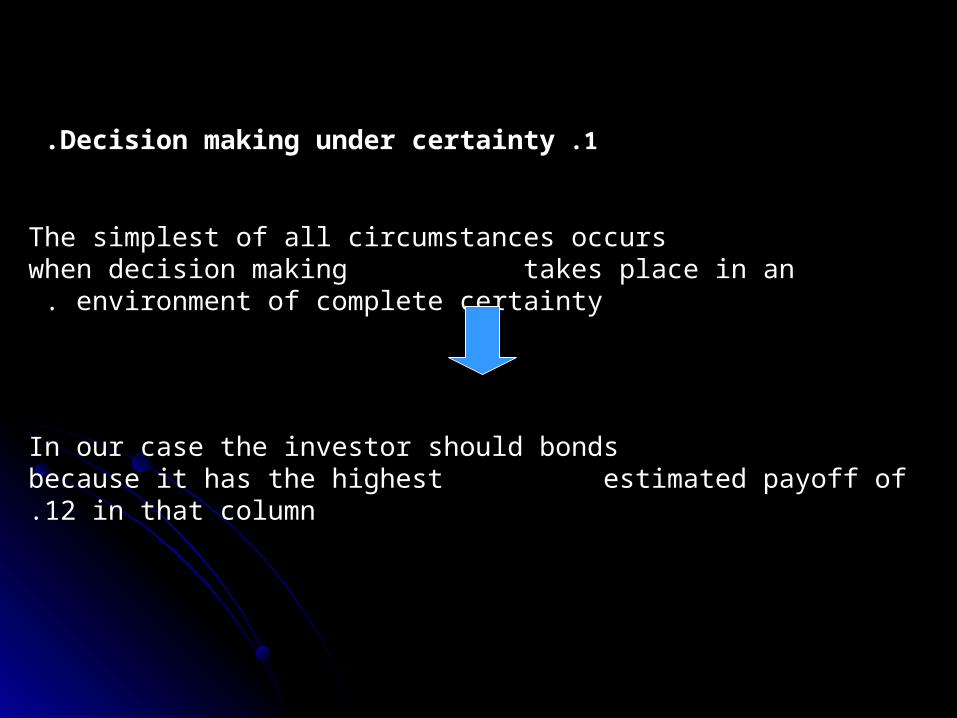
1 .Decision making under certainty.
The simplest of all circumstances occurs when decision making takes place in an environment of complete certainty .
In our case the investor should bonds because it has the highest estimated payoff of 12 in that column.
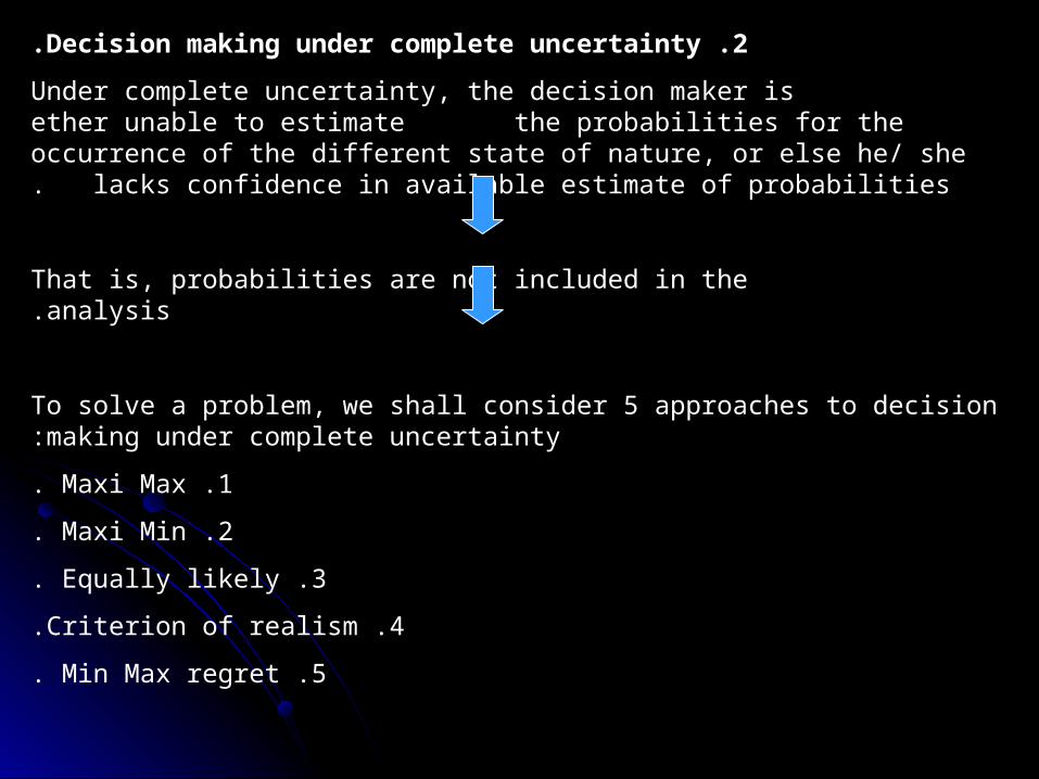
2 .Decision making under complete uncertainty.
Under complete uncertainty, the decision maker is ether unable to estimate the probabilities for the occurrence of the different state of nature, or else he/ she lacks confidence in available estimate of probabilities.
That is, probabilities are not included in the analysis.
To solve a problem, we shall consider 5 approaches to decision making under complete uncertainty:
1 .Maxi Max.
2 .Maxi Min.
3 .Equally likely.
4 .Criterion of realism.
5 .Min Max regret.
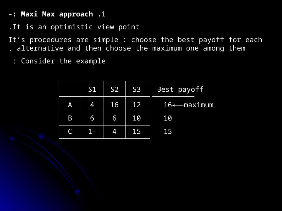
1 .Maxi Max approach-:
It is an optimistic view point.
It’s procedures are simple : choose the best payoff for each alternative and then choose the maximum one among them.
Consider the example :
4 16 12
6 6 10
-1 4 15
A
B
C
S1 S2 S3 Best payoff
16
10
15
maximum
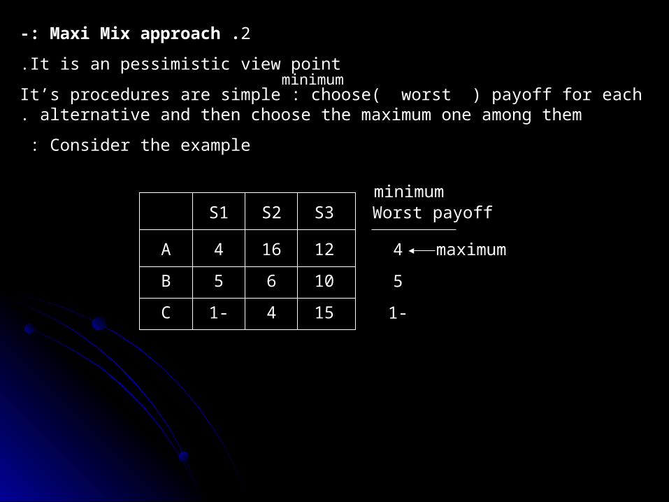
2 .Maxi Mix approach-:
It is an pessimistic view point.
It’s procedures are simple : choose( worst ) payoff for each alternative and then choose the maximum one among them.
Consider the example :
minimum
4 16 12
5 6 10
-1 4 15
A
B
C
S1 S2 S3 Worst payoff
4
5
-1
maximum
minimum
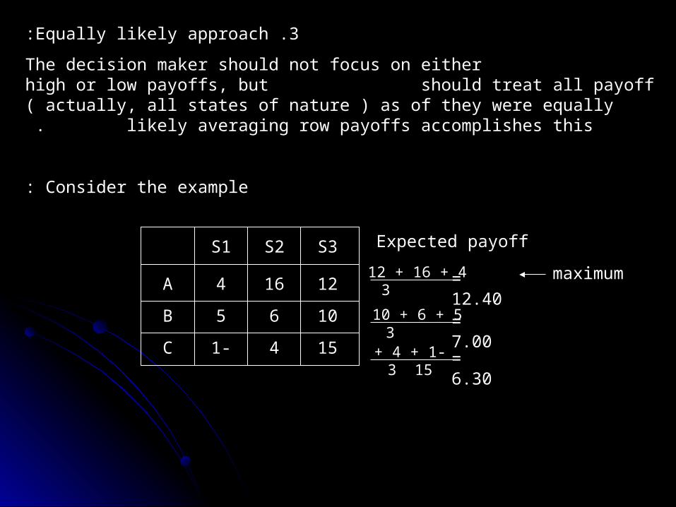
3 .Equally likely approach:
The decision maker should not focus on either high or low payoffs, but should treat all payoff ( actually, all states of nature ) as of they were equally
likely averaging row payoffs accomplishes this .
Consider the example:
4 16 12
5 6 10
-1 4 15
A
B
C
S1 S2 S3 Expected payoff
4 + 16 + 12 3
5 + 6 + 10 3
-1 + 4 + 15 3
maximum = 12.40
= 7.00
= 6.30
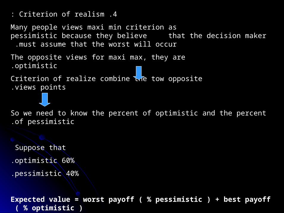
4 .Criterion of realism:
Many people views maxi min criterion as pessimistic because they believe that the decision maker must assume that the worst will occur .
The opposite views for maxi max, they are optimistic.
Criterion of realize combine the tow opposite views points.
So we need to know the percent of optimistic and the percent of pessimistic.
Suppose that
60% optimistic.
40% pessimistic.
Expected value = worst payoff ( % pessimistic ) + best payoff ( % optimistic )
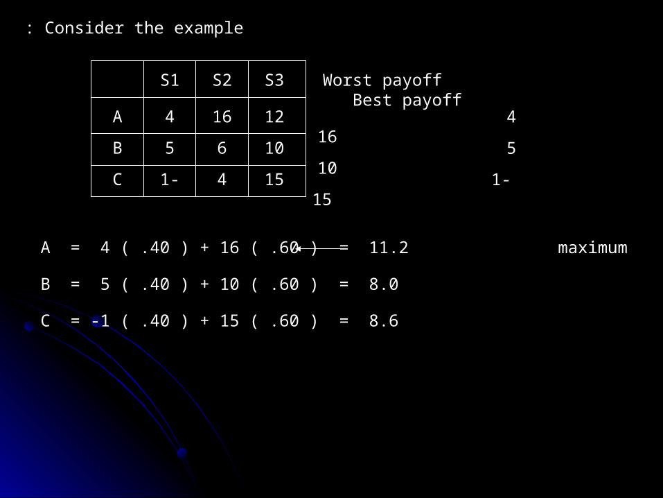
Consider the example:
4 16 12
5 6 10
-1 4 15
A
B
C
S1 S2 S3 Worst payoff Best payoff
4 16
5 10
- 1 15
A = 4 ( .40 ) + 16 ( .60 ) = 11.2 maximum
B = 5 ( .40 ) + 10 ( .60 ) = 8.0
C = -1 ( .40 ) + 15 ( .60 ) = 8.6
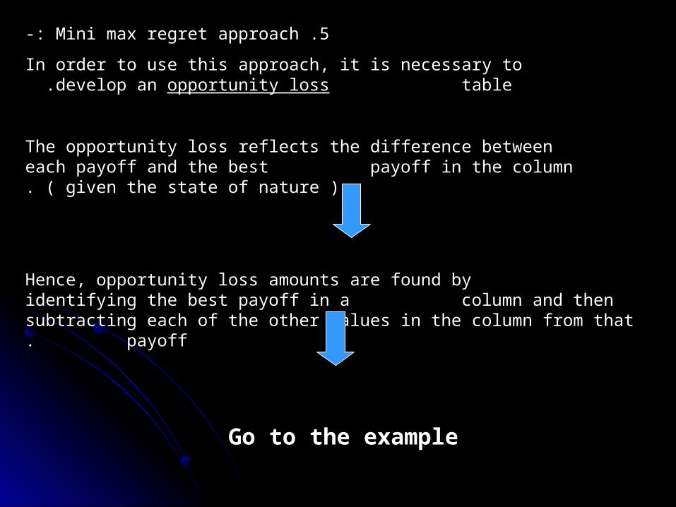
5 .Mini max regret approach-:
In order to use this approach, it is necessary to develop an opportunity loss table .
The opportunity loss reflects the difference between each payoff and the best payoff in the column ( given the state of nature ).
Hence, opportunity loss amounts are found by identifying the best payoff in a column and then subtracting each of the other values in the column from that payoff.
Go to the example
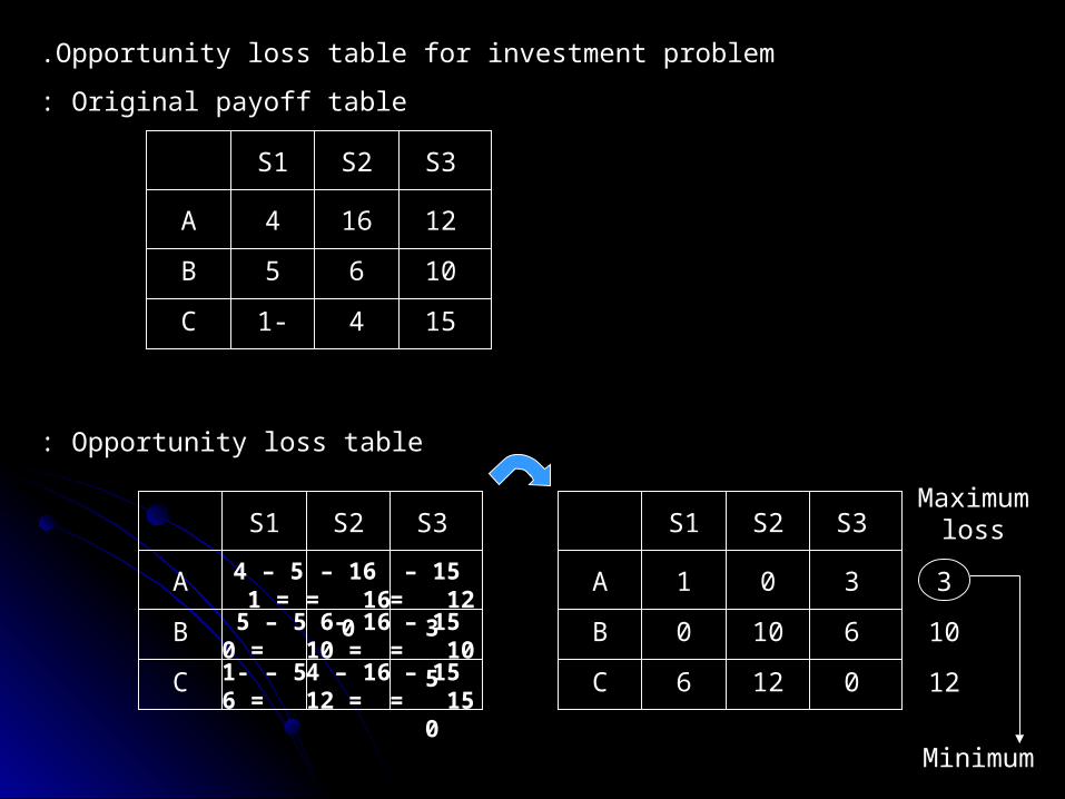
Opportunity loss table for investment problem.
Original payoff table:
Opportunity loss table:
4 16 12
5 6 10
-1 4 15
A
B
C
S1 S2 S3
5 – 4 =1
A
B
C
S1 S2 S3
16 – 16 =0
15 – 12 =3
5 – 5 =0
16– 6 =10
15 – 10 =5
5- – 1 =6
16 – 4 =12
15 – 15 =0
1 0 3
0 10 6
6 12 0
A
B
C
S1 S2 S3Maximum
loss
3
10
12
Minimum
3 .Decision making under risk.
The essential difference between decision making under complete uncertainty and decision making partial uncertainty ( risk ) is the presence of probabilities.
Under risk the manager know the probabilities for the occurrence of various state of natures.
1 .The probabilities may be subjective estimates from manager, or
2 .From experts in a particular field , or.
3 .They may reflect historical frequencies.
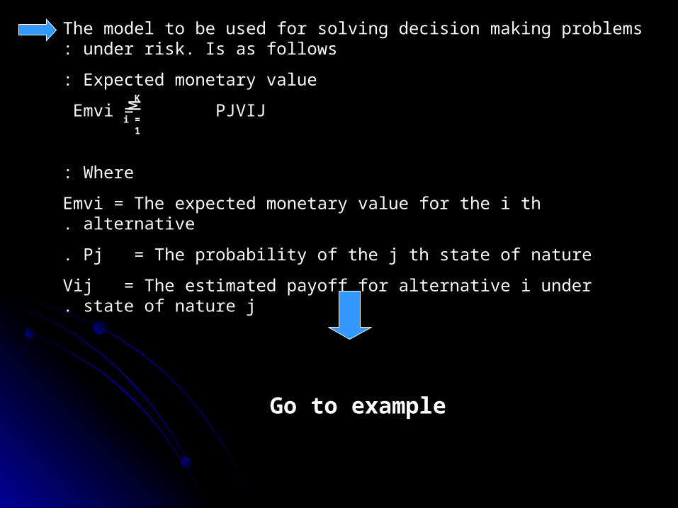
The model to be used for solving decision making problems under risk. Is as follows:
Expected monetary value:
Emvi = PJVIJ
Where:
Emvi = The expected monetary value for the i th alternative.
Pj = The probability of the j th state of nature.
Vij = The estimated payoff for alternative i under state of nature j.
Go to example
Mi = 1
K
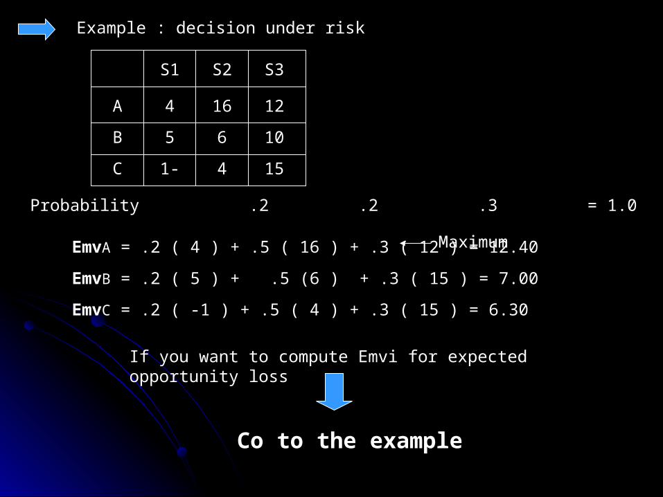
Example : decision under risk
4 16 12
5 6 10
-1 4 15
A
B
C
S1 S2 S3
Probability .2 .2 .3 = 1.0
EmvA = .2 ( 4 ) + .5 ( 16 ) + .3 ( 12 ) = 12.40
EmvB = .2 ( 5 ) + .5 (6 ) + .3 ( 15 ) = 7.00
EmvC = .2 ( -1 ) + .5 ( 4 ) + .3 ( 15 ) = 6.30
If you want to compute Emvi for expected opportunity loss
Co to the example
Maximum
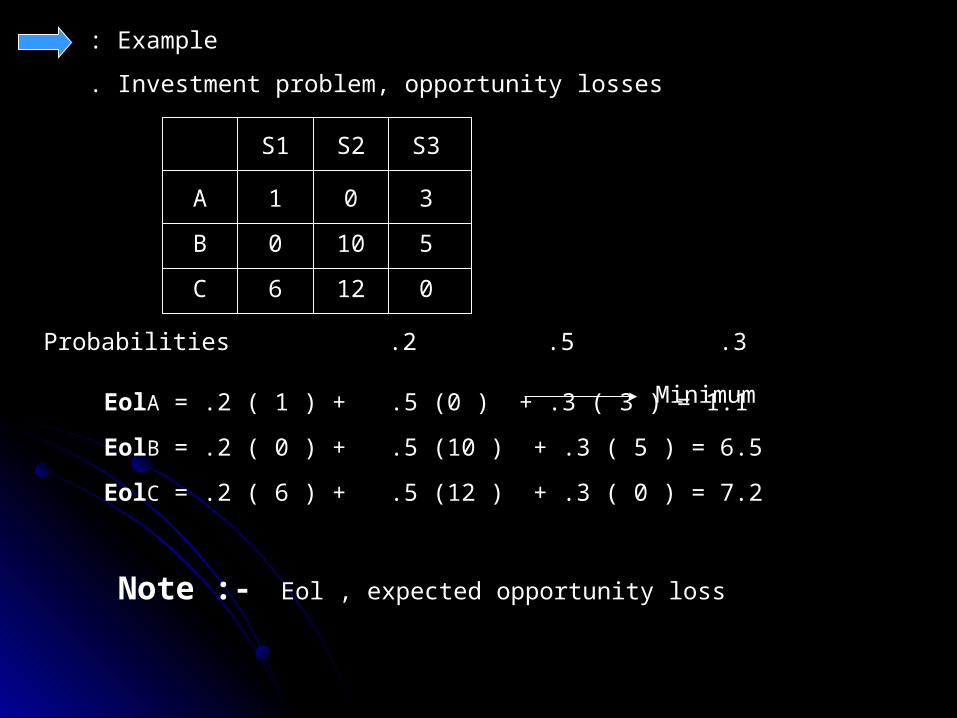
Example:
Investment problem, opportunity losses.
1 0 3
0 10 5
6 12 0
A
B
C
S1 S2 S3
Probabilities .2 .5 .3
EolA = .2 ( 1 ) + .5 (0 ) + .3 ( 3 ) = 1.1
EolB = .2 ( 0 ) + .5 (10 ) + .3 ( 5 ) = 6.5
EolC = .2 ( 6 ) + .5 (12 ) + .3 ( 0 ) = 7.2
Minimum
Note :- Eol , expected opportunity loss
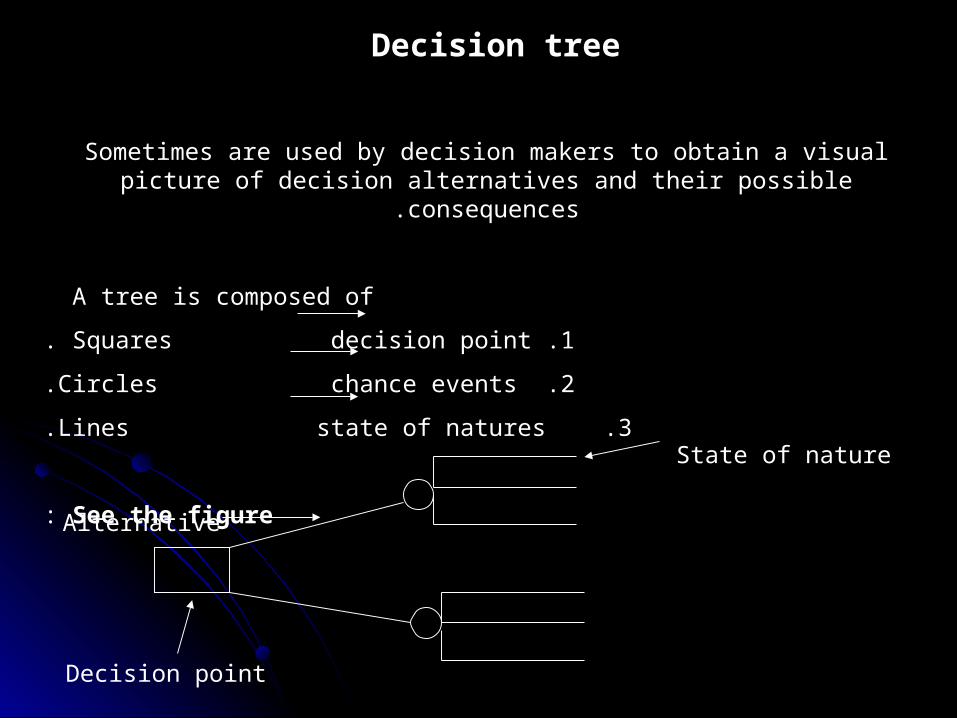
Decision tree
Sometimes are used by decision makers to obtain a visual picture of decision alternatives and their possible consequences.
A tree is composed of
1 .Squares decision point.
2 .Circles chance events.
3 .Lines state of natures .
See the figure:
State of nature
Alternative
Decision point
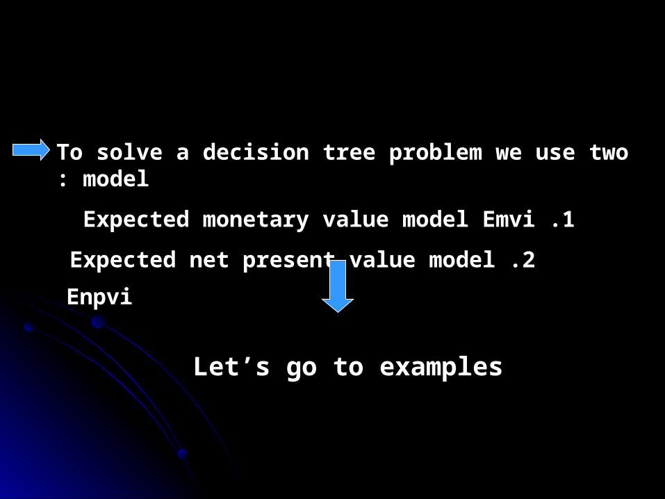
To solve a decision tree problem we use two model:
1 .Expected monetary value model Emvi
2 .Expected net present value model
Enpvi
Let’s go to examples
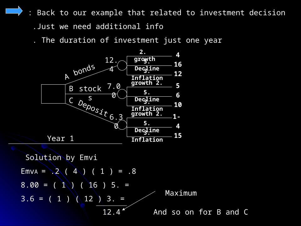
Back to our example that related to investment decision:
Just we need additional info .
The duration of investment just one year .
. 2 growth
.5 Decline
.3 Inflation
4
16
12.2 growth
.5 Decline
.3 Inflation
5
6
10.2 growth
.5 Decline
.3 Inflation
-1
4
15
12.4
7.00
6.30
A
B
C
bonds
stocks
Deposit
1 Year
Solution by Emvi
EmvA = .2 ( 4 ) ( 1 ) = .8
. = 5 ) 16 ) ( 1 = ( 8.00
. = 3 ) 12 ) ( 1 = ( 3.6
12.4
Maximum
And so on for B and C
Using Enpvi to solve decision tree problems.
Note -:
1 .You need to have with you net present value tables single, and annuity tables. And you can use them.
Or
2 .You need to have net present value equations and you can apply it.
Let’s go examples
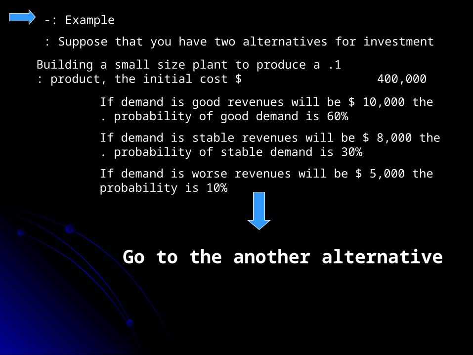
Example-:
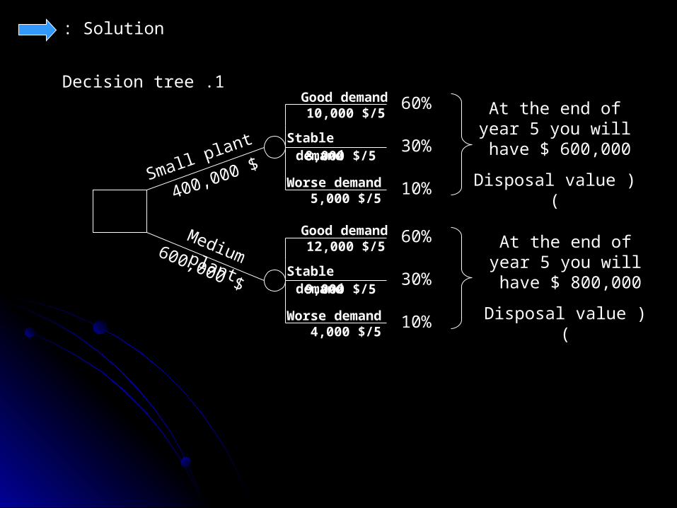
Suppose that you have two alternatives for investment:
1 .Building a small size plant to produce a product, the initial cost $ 400,000:
If demand is good revenues will be $ 10,000 the probability of good demand is 60%.
If demand is stable revenues will be $ 8,000 the probability of stable demand is 30%.
If demand is worse revenues will be $ 5,000 the probability is 10%
Go to the another alternative
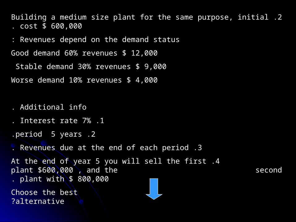
2 .Building a medium size plant for the same purpose, initial cost $ 600,000.
Revenues depend on the demand status:
Good demand 60% revenues $ 12,000
Stable demand 30% revenues $ 9,000
Worse demand 10% revenues $ 4,000
Additional info.
1 .Interest rate 7%.
2 .period 5 years.
3 .Revenues due at the end of each period.
4 .At the end of year 5 you will sell the first plant $600,000 , and the second plant with $ 800,000.
Choose the best alternative?
Go to the solution.
Solution:
Small plant
Medium plant
1 .Decision tree Good demand
5 $/10,000
Stable demand 5 $/8,000
Worse demand 5 $/5,000
60%
30%
10%
Good demand 5 $/12,000
Stable demand 5 $/9,000
Worse demand 5 $/4,000
60%
30%
10%
$400,000
$
600,000
At the end of year 5 you will have $
600,000
)Disposal value(
At the end of year 5 you will have $
800,000
)Disposal value(
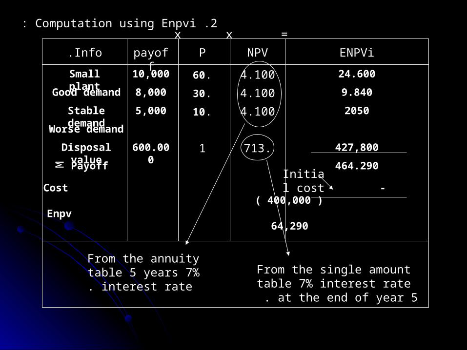
2 .Computation using Enpvi:
Info. payoff P NPV ENPVi
x x =
Small plant 10,000 .60 4.100 24.600
Good demand 8,000 .30 4.100 9.840
Stable demand 5,000 .10 4.100 2050
Worse demand
Disposal value 600.000 1 .713 427,800
Payoff M 464.290
- Cost ( 400,000 )
Enpv 64,290
Initial cost
From the annuity table 5 years 7% interest rate. From the single amount table
7% interest rate at the end of year 5 .
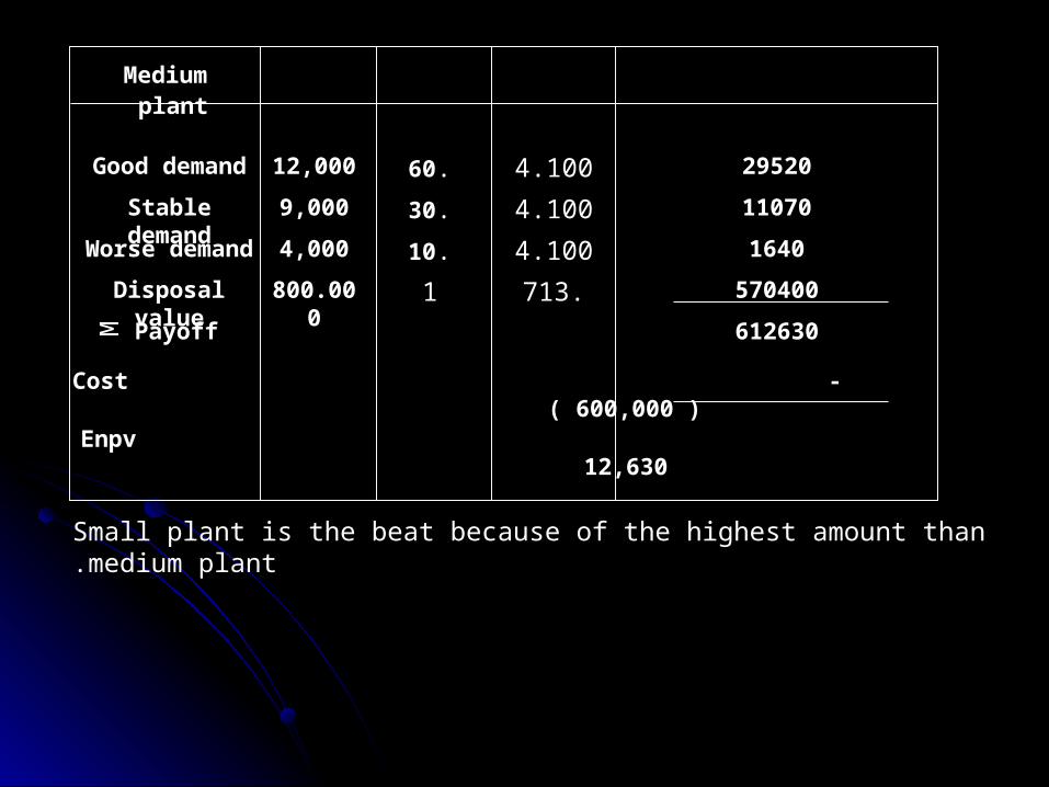
Medium plant
Good demand 12,000 .60 4.100 29520
Stable demand 9,000 .30 4.100 11070
Worse demand
Disposal value 800.000 1 .713 570400
Payoff M 612630
- Cost ( 600,000 )
Enpv 12,630
4,000 .10 4.100 1640
Small plant is the beat because of the highest amount than medium plant.
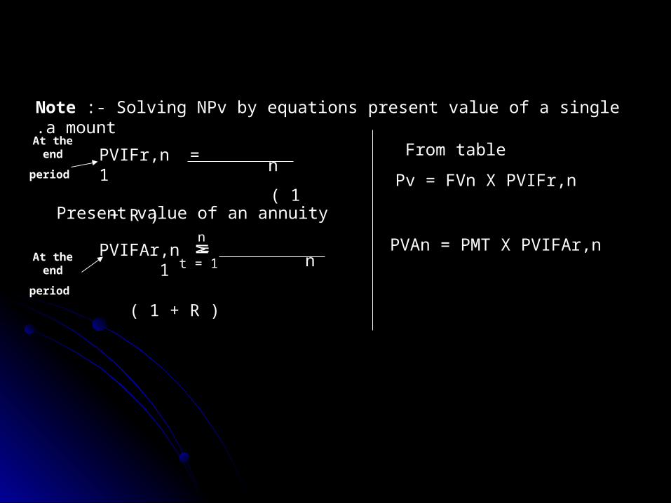
Note :- Solving NPv by equations present value of a single a mount.
PVIFr,n = 1 ( 1 + R )
n
Present value of an annuity
PVIFAr,n = 1 ( 1 + R )
n
M
n
t = 1
At the end
period
At the end
period
From table
Pv = FVn X PVIFr,n
PVAn = PMT X PVIFAr,n
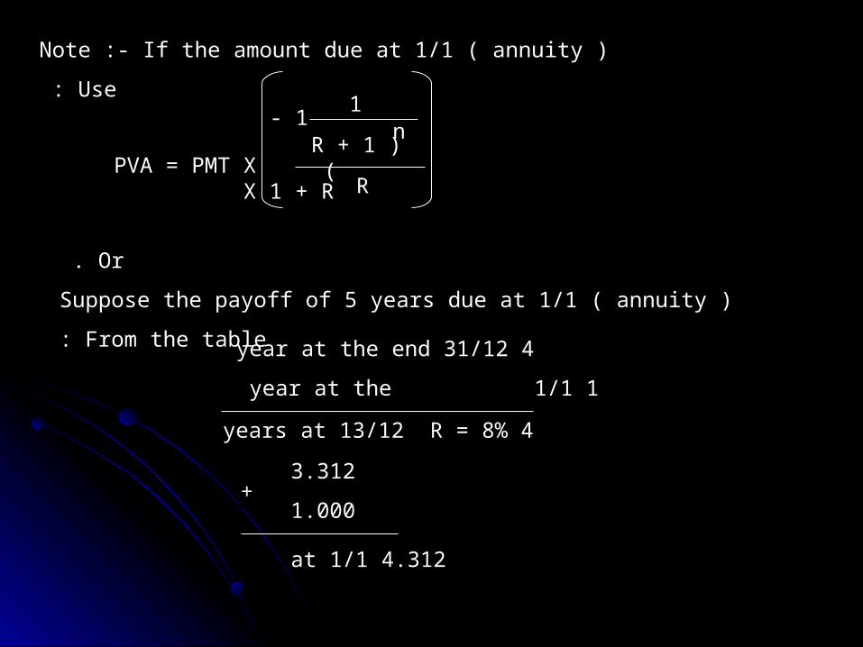
Note :- If the amount due at 1/1 ( annuity )
Use :
PVA = PMT X X 1 + R R
1 - 1
)1 + R ( n
Or .
Suppose the payoff of 5 years due at 1/1 ( annuity )
From the table: 4 year at the end 31/12
1 year at the 1/1
4 years at 13/12 R = 8%
3.312
1.000+
4.312 at 1/1