Ch 3-1 Limits

Slide 1-2

THE LIMIT (L) OF A FUNCTION IS THE VALUE THE FUNCTION (y) APPROACHES AS THE VALUE OF (x) APPROACHES A GIVEN VALUE.

ax Lxf )(lim

Slide 1-3

Direct Substituion

•Easiest way to solve a limit•Can’t use if it gives an undefined answer

Slide 1-4

Table method and direct substitution method.

3lim ?x 2x

because as x gets closer and closerto 2, x cubed gets closer and closerto 8. (graphically on next slide)

Slide 1-5

Slide 1-6

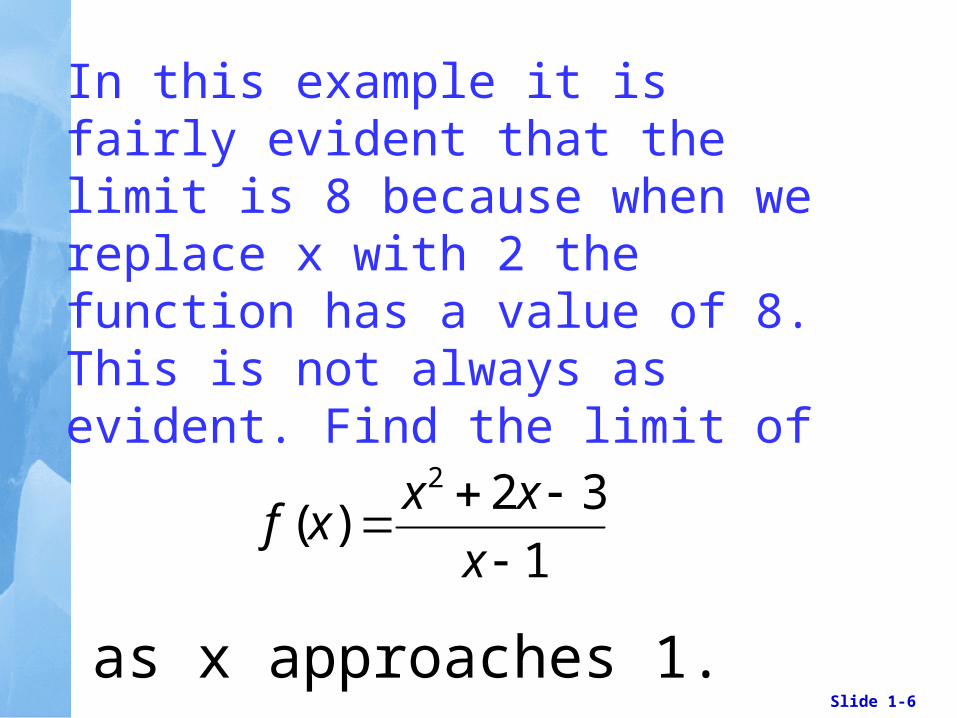
In this example it is fairly evident that the limit is 8 because when we replace x with 2 the function has a value of 8. This is not always as evident. Find the limit of

1

32)(

2

x

xxxf

as x approaches 1.

Slide 1-7

Rewrite before substituting

Factor and cancel common factors – then do direct substitution.

The answer is 4.

Slide 1-8

means x approaches a from the right and

means x approaches a from the left

ax

ax

Slide 1-9

When finding the limit of a function it is important to let x approach a from both the right and left. If the same value of L is approached by the function then the limit exist and

Lxf )(limax

Slide 1-10

THEOREM:As x approaches a, the limit of f (x) is L, if the limit from the left exists and the limit from the right exists and both limits are L. That is, if

1)

and 2)

then

limx a

f (x) L,

limx a

f (x) L,

limx a

f (x) L,

Slide 1-11

Graphs can be used to determine the limit of a function. Find the following limits.

1

1lim

2

x

x1x

Slide 1-12

a) Limit GraphicallyObserve on the graph

that: 1)

and 2)

Therefore, does not exist.

limx1

H (x) 4

limx1

H (x) 2

limx1

H (x)

1.1 Limits: A Numerical and Graphical Approach

Slide 1-13

The “Wall” Method:As an alternative approach to Example 1, we can draw a “wall” at x = 1, as shown in blue on the following graphs. We then follow the curve from left to rightwith pencil until we hit the wall and mark the locationwith an × , assuming it can be determined. Then we follow the curve from right to left until we hit the walland mark that location with an ×. If the locations arethe same, we have a limit. Otherwise, the limit does not exist.

1.1 Limits: A Numerical and Graphical Approach

Slide 1-14

Thus for Example 1:

does not exist limx 3

H (x) 4limx1

H (x)

1.1 Limits: A Numerical and Graphical Approach

Slide 1-15

a) Limit GraphicallyObserve on the graph

that: 1)

and 2)

Therefore,

limx 3

f (x) 4

limx 3

f (x) 4

limx 3

f (x) 4.

1.1 Limits: A Numerical and Graphical Approach

Slide 1-16

We can also use Derive to evaluate limits.

Slide 1-17

Use Derive to find the indicated limit.

12204 25

0lim

xxxx

3

22

2 4

1limx

x

x

3

92

3lim

x

x

x

Slide 1-18

Limits at infinitySometimes we will be concerned with the value of a function as the value of x increases without bound. These cases are referred to as limits at infinity and are denoted

( ) and ( )lim limx x

f x f x

Slide 1-19

For polynomial functions the limit will be + or - infinity as demonstrated by the end behavior of the leading term.

Slide 1-20

For rational functions, the limit at infinity is the same as the horizontal asymptote (y = L) of the function. Recall the method of finding the horizontal asymptote depends on the degrees of the numerator and denominator

Slide 1-21Copyright © 2008 Pearson Education, Inc. Publishing as

Pearson Addison-Wesley

Slide 1.1- 21

Limit GraphicallyObserve on the graph

that,again, you can only approach ∞ from the left.

Therefore,

limx

f (x) 3.

1.1 Limits: A Numerical and Graphical Approach

Slide 1-22

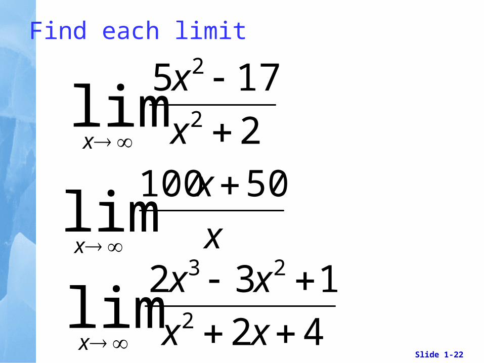
Find each limit

x

x

x

50100lim

42

1322

23

lim

xx

xx

x

2

1752

2

lim

x

x

x

Slide 1-23

Infinite limits

When considering f(x) may increase or decrease without bound (becomes infinite) as x approaches a. In these cases the limit is infinite and

)(lim xfax

)(lim xfax

Slide 1-24

b) Limit GraphicallyObserve on the graph

that: 1)

and 2)

Therefore, does not exist.

limx 2

f (x)

limx 2

f (x)

limx 2

f (x)

1.1 Limits: A Numerical and Graphical Approach

Slide 1-25

When this occurs the line x = a is a vertical asymptote.

Polynomial functions do not have vertical asymptotes, but rational functions have vertical asymptotes at values of x that make the denominator = 0.

Slide 1-26

Find each limit.

xx

3lim

0 1

3lim

1 xx

1

3lim

1 xx

Slide 1-27

The cost (in dollars) for manufacturing a particular videotape is

xxC 615000)(

)(xC

lim ( )x

C x

where x is the number of tapesproduced. The average cost pertape, denoted by is foundby dividing C(x) by x. Find and interpret