Embed Size (px)
Citation preview
49th AIAA Aerospace Sciences Meeting, Jan. 4–7, 2011, Orlando, Fl
Best Practices for CFD Simulations of Launch Vehicle
Ascent with Plumes - OVERFLOW Perspective
Marshall Gusman∗, Jeffrey Housman
∗
ELORET Corporation, 465 S. Mathilda Ave. Suite 103, Sunnyvale, CA 94086
Cetin Kiris†
NASA Ames Research Center, Moffett Field, CA 94035
A simulation protocol has been developed for modeling rocket plumes of heavy liftlaunch vehicles (HLLV) during ascent. The procedure uses a series of sensitivity studiesapplied to the Saturn V launch vehicle to establish accurate plume physics modeling ofHLLV main engines. These analyses include a comparison of calorically and thermallyperfect gas models, a grid dependence study, a sensitivity analysis of nozzle exit boundaryconditions for both single and multi-species gas assumptions, and a thorough turbulencemodel sensitivity study. The results of the analyses are assessed by comparing the pre-dicted plume induced flow separation (PIFS) distance, an important quantity for thermalprotection system design. This quantity is also used to validate the results with exist-ing flight data. The viscous Computational Fluid Dynamics (CFD) code OVERFLOW, aReynolds Averaged Navier-Stokes flow solver for structured overset grids is utilized. Thiswork is a continuation of the CFD best practices for Ares V aero-database simulation,1
with the additional complexity of plume physics modeling.
Nomenclature
D : Reference diameter, mReD : Reynolds number based on DM∞ : Free-stream Mach numberP∞ : Free-stream pressure, PaT∞ : Free-stream temperature, ◦Kρ : Density, kg/m3
c : Speed of sound, m/sT : Temperature, ◦Ky+ : Non-dimensional wall spacingPIFS : Plume-induced flow separationSA : Spalart Allmaras 1-equation turbulence modelSST : Shear-Stress Transport 2-Equation Turbulence modelSST-00 : SST turbulence model with no correctionsSST-10 : SST turbulence model with curvature correctionSST-01 : SST turbulence model with temperature correctionSST-11 : SST turbulence model with curvature and temperature correction
∗Aerospace Engineer†Branch Chief
1 of 15
American Institute of Aeronautics and Astronautics
I. Introduction
High-fidelity modeling and simulation is currently being used in NASA’s development of next generationlaunch vehicles, including a Heavy Lift Launch Vehicle (HLLV) for carrying large payloads to low earth orbit.The best practice protocol provides information on the necessary mesh resolution requirements, physicalmodels, boundary conditions, and turbulence models to accurately predict the quantities of interest. Inthe context of HLLV ascent, some of the quantities of interest include aerodynamic force and momentcoefficients and load distributions, as well as base heating and surface pressure estimates. To provideacceptable predictions of these quantities, the CFD simulations must accurately model the physics of theexhaust plume as it expands with increasing altitude. The purpose of this study is to investigate the CFDrequirements to accomplish this goal, as a first step in developing current CFD practices for plumes. Thiswork, along with work in USM3D,2 is a continuation of the CFD best practices for aero-database generationof Ares V during ascent, Kiris et al.1
Rockets at high-altitude are subject to a fluid dynamics phenomenon known as Plume-Induced FlowSeparation3 (PIFS). Flow separation occurs when an adverse pressure gradient forces the boundary layerto detach from the surface of the rocket. One cause of the adverse pressure gradient during ascent is theexpansion of the exhaust plume as the rocket gains altitude. In a low ambient pressure environment, thehigh pressure at the nozzle exit rapidly expands the exhaust jet in both downstream and radial directions.This produces an obstruction to the free-stream flow which forms an adverse pressure gradient near the aftsection of the rocket. Ultimately, the flow separates and recirculation from the base of the vehicle to theupstream separation point allows convective transport of hot exhaust gas along the surface of the vehicle.The distance between the end of the vehicle and the separation point of the surface is denoted as the PIFSdistance. Accurate prediction of the PIFS distance is critical to the design of the thermal protection system,and will be used in this study to quantify the accuracy of the computed results. The purpose of this work isto demonstrate, through a series of sensitivity studies, the modeling and simulation requirements for accurateplume physics modeling and PIFS distance prediction of HLLVs during ascent. The Saturn V launch vehicleis used in this study as a representative HLLV, and flight data from the launch of Apollo 11 is used tovalidate the computed results.
In this paper, a preliminary study is performed to compare plume modeling for two multi-species gasmodels. This two-dimensional axisymmetric jet expansion problem was performed with the commercialCFD software, Star-CCM+,4 to evaluate the calorically perfect gas assumption used in the NASA-developedCFD code OVERFLOW.5 OVERFLOW is a viscous Reynolds Averaged Navier-Stokes (RANS) flow solverfor high Reynolds number turbulent flows using structured overset grids. OVERFLOW is used to performall three-dimensional plume simulations reported in this paper. A series of sensitivity and validation stud-ies are performed to determine the best practices for plume simulations and predictions of PIFS. Thesestudies include a near-wall grid resolution study, sensitivity analysis of nozzle exit boundary conditions formulti-species flow models, a comparison between the multi-species gas model and single species gas model as-sumptions, and a detailed turbulence modeling sensitivity study. Best practices resulting from these studiesare summarized in the conclusion.
The current work builds on the knowledge and experience attained through previous studies on otherlaunch vehicles. These studies include work on the Space Shuttle,6 best practices for overset grid generation,7best practices for Orion,8 and best practices for ascent aerodynamics of Ares I.9
II. Problem Description
Simulations in this paper are performed using the Saturn V launch vehicle during ascent, with theinclusion of exhaust plume effects. Saturn V is an Apollo-era launch vehicle, with a vertical-stack designthat resembles design concepts for future heavy lift launch vehicles currently being developed at NASA. Datafor the Saturn V’s trajectory, geometry, and flight performance is publicly available, along with flight datasuch as PIFS distance. All flight trajectory information is derived from the Flight Evaluation report fromthe launch of Apollo 11.10
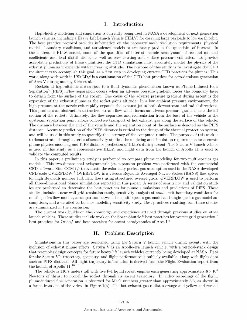
The vehicle is 110.7 meters tall with five F-1 liquid rocket engines each generating approximately 8× 10⁶
Newtons of thrust to propel the rocket through its ascent trajectory. In video recordings of the flight,plume-induced flow separation is observed for Mach numbers greater than approximately 3.3, as shown ina frame from one of the videos in Figure 1(a). The hot exhaust gas radiates orange and yellow and reveals
2 of 15
American Institute of Aeronautics and Astronautics
the extent of plume induced flow separation up the sides of the vehicle. PIFS distance measurements weremade from video footage of the launch, and contain an uncertainty of approximately 10%. At Mach 4.4,PIFS was measured at 15 meters from the vehicle reference station 0, see Figure 1(b) for a diagram of PIFSmeasurements. To reduce loads on the vehicle and crew, the center engine cut-off (CECO) event occursat 136 seconds, leading to a brief reduction in PIFS distance before it climbs back to 33 meters at Mach6.5. Steady-state simulations were performed at four points in the ascent trajectory with correspondingsupersonic Mach numbers 1.5, 2.7, 4.4, and 6.5. A description of the flow solvers used in this study ispresented in the next section.
Table 1. Free-stream conditions for Saturn V PIFS simulations.
M∞ P∞ (Pa) T∞ (◦K) ReD
1.5 12111.0 217 6.1522×10⁷
2.7 2250.0 221 2.2623×10⁷
4.4 151.0 264 1.6970×10⁶
6.5 22.0 247 4.0600×10⁵
(a) (b)
Figure 1. PIFS examples: (a) frame from chase plane footage of Apollo 6 flight with PIFS visible by extent
of radiating exhaust gas, and (b) diagram of Saturn V station zero (located 2.8 m from the nozzle exit) and
measurement of PIFS distance.
III. CFD Solvers
A. OVERFLOW
The NASA flow solver OVERFLOW-2 is used to simulate the viscous flow field around the Saturn V launchvehicle with exhaust plumes. OVERFLOW is an implicit structured overset Reynolds-Averaged Navier-Stokes (RANS) solver for structured overset grids. Second-order central-differencing with explicit artificialdissipation is used for the convective fluxes. The Beam-Warming block tri-diagonal implicit ADI scheme isrun in parallel using domain decomposition and the Message Passing Interface (MPI) standard. The solverwas run on the Columbia and Pleiades supercomputers at NASA Ames Research Center, using 128 processors
3 of 15
American Institute of Aeronautics and Astronautics
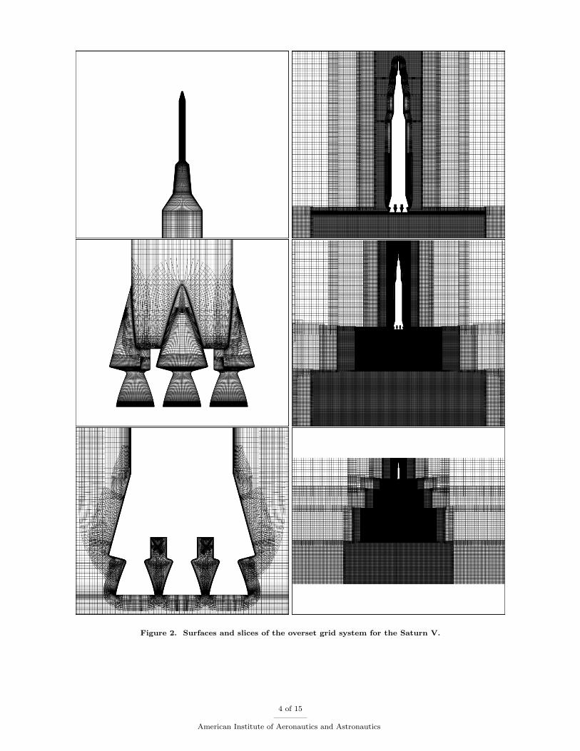
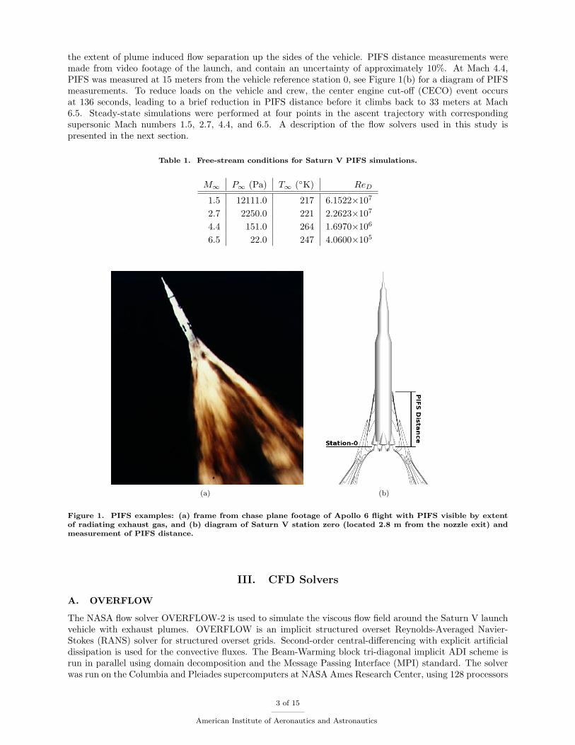
Figure 2. Surfaces and slices of the overset grid system for the Saturn V.
4 of 15
American Institute of Aeronautics and Astronautics
and approximately 36 hours of runtime for each steady state run. Structured viscous overset grid systemswere built to represent the geometry of the Saturn V flight vehicle using grid generation scripts based on theChimera Grid Tools (CGT) script library.11 The overset grid system for Saturn V, see Figure 2, contains 67zones and approximately 52-60 million grid points. A hierarchy of successively refined cylindrical off-bodygrids are used to discretize the external domain. The off-body grids shown on the right of Figure 2 werecreated in the plume region to maintain high resolution for all points in the trajectory. Using cylindricalgrids allows the plume to remain well-resolved in the off-body using fewer mesh points than a Cartesianoff-body grid system. Typical convergence results are shown in Figure 3, where the residual convergenceis plotted on the left and the force convergence is plotted on the right. The large spikes in the earlystages of the residual plot are caused by a successive reduction of the artificial dissipation parameters fromrelatively large values to the default values described in the OVERFLOW manual, see Ref. 5. Modifyingthe dissipation parameters during the development of the steady solution allows the use of a large CFLnumber throughout the computations, and leads to overall faster convergence of the problem. The nozzleexit boundary conditions used for the simulations are described in detail in Section V.
Figure 3. Convergence history of the OVERFLOW residuals (left) and forces (right) for the Saturn V.
B. Star-CCM+
The commercial software package Star-CCM+ is used to compare the calorically perfect gas assumption withthe thermally perfect gas model for simulations of plume expansion. Star-CCM+ is an unstructured poly-hedral finite-volume Navier-Stokes flow solver. The code is made parallel using domain decomposition andMPI message passing. The inviscid fluxes are discretized using Roe flux difference splitting12 with MUSCLextrapolation and central-differencing for the viscous fluxes. An implicit point Gauss-Seidel procedure isused to iterate to steady-state along with algebraic multigrid for convergence acceleration.
IV. Plume Physics
The exhaust plume emitted from a liquid rocket engine is a complex flow field composed of a chemicallyreacting mixture of gases and unburned liquid fuel. In Table 2, five categories of plume physics modelingare described in descending levels of complexity. Each model is listed with its requirements, limitations, andexamples of available CFD software that have implementations of the model. The best practices for CFDsupport of HLLV design requires accurate predictions of flow phenomena such as PIFS distance. For efficientuse of computational resources, the least expensive model which predicts the relevant quantities of interestshould be used. The two most commonly implemented and tested choices are the single-species perfectgas model and the calorically perfect multi-species model, both of which are available in OVERFLOW. Todetermine the differences between the calorically perfect and thermally perfect multi-species gas assumptionson modeling plume expansion, Star-CCM+ was applied to a two-dimensional axisymmetric nozzle case usingthese two different gas models.
5 of 15
American Institute of Aeronautics and Astronautics
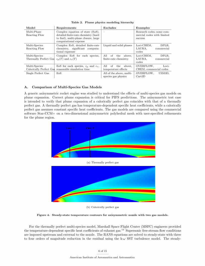
Table 2. Plume physics modeling hierarchy
Model Requirements Excludes Examples
Multi-PhaseReacting Flow
Complex equation of state (EoS),detailed finite-rate chemistry (hardto find), multi-phase closure, largecomputational expense
– Research codes, some com-mercial codes with limitedsuccess
Multi-SpeciesReacting Flow
Complex EoS, detailed finite-ratechemistry, significant computa-tional expsense
Liquid and solid phases Loci-CHEM, DPLR,LAURA, commercialcodes
Multi-SpeciesThermally Perfect Gas
Complex EoS for each species,cp(T ) and cv(T )
All of the above,finite-rate chemistry
Loci-CHEM, DPLR,LAURA, commercialcodes
Multi-SpeciesCalorically Perfect Gas
EoS for each species, cp and cv ,reasonable simulation time
All of the above,temperature effects
OVERFLOW, Loci-CHEM, commercial codes
Single Perfect Gas EoS All of the above, multi-species gas physics
OVERFLOW, USM3D,Cart3D
A. Comparison of Multi-Species Gas Models
A generic axisymmetric rocket engine was studied to understand the effects of multi-species gas models onplume expansion. Correct plume expansion is critical for PIFS predictions. The axisymmetric test caseis intended to verify that plume expansion of a calorically perfect gas coincides with that of a thermallyperfect gas. A thermally perfect gas has temperature-dependent specific heat coefficients, while a caloricallyperfect gas assumes constant specific heat coefficients. The gas models are compared using the commercialsoftware Star-CCM+ on a two-dimensional axisymmetric polyhedral mesh with user-specified refinementsfor the plume region.
(a) Thermally perfect gas
(b) Calorically perfect gas
Figure 4. Steady-state temperature contours for axisymmetric nozzle with two gas models.
For the thermally perfect multi-species model, Marshall Space Flight Center (MSFC) engineers providedthe temperature-dependent specific heat coefficients of exhaust gas.13 Supersonic free-stream flow conditionsare imposed upstream and external to the nozzle. The RANS equations are solved to steady-state with threeto four orders of magnitude reduction in the residual using the k-ω SST turbulence model. The steady-
6 of 15
American Institute of Aeronautics and Astronautics
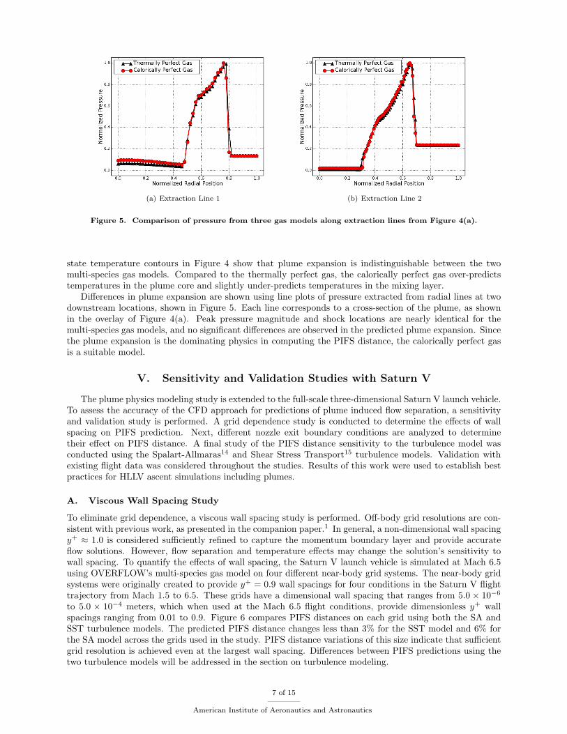
(a) Extraction Line 1 (b) Extraction Line 2
Figure 5. Comparison of pressure from three gas models along extraction lines from Figure 4(a).
state temperature contours in Figure 4 show that plume expansion is indistinguishable between the twomulti-species gas models. Compared to the thermally perfect gas, the calorically perfect gas over-predictstemperatures in the plume core and slightly under-predicts temperatures in the mixing layer.
Differences in plume expansion are shown using line plots of pressure extracted from radial lines at twodownstream locations, shown in Figure 5. Each line corresponds to a cross-section of the plume, as shownin the overlay of Figure 4(a). Peak pressure magnitude and shock locations are nearly identical for themulti-species gas models, and no significant differences are observed in the predicted plume expansion. Sincethe plume expansion is the dominating physics in computing the PIFS distance, the calorically perfect gasis a suitable model.
V. Sensitivity and Validation Studies with Saturn V
The plume physics modeling study is extended to the full-scale three-dimensional Saturn V launch vehicle.To assess the accuracy of the CFD approach for predictions of plume induced flow separation, a sensitivityand validation study is performed. A grid dependence study is conducted to determine the effects of wallspacing on PIFS prediction. Next, different nozzle exit boundary conditions are analyzed to determinetheir effect on PIFS distance. A final study of the PIFS distance sensitivity to the turbulence model wasconducted using the Spalart-Allmaras14 and Shear Stress Transport15 turbulence models. Validation withexisting flight data was considered throughout the studies. Results of this work were used to establish bestpractices for HLLV ascent simulations including plumes.
A. Viscous Wall Spacing Study
To eliminate grid dependence, a viscous wall spacing study is performed. Off-body grid resolutions are con-sistent with previous work, as presented in the companion paper.1 In general, a non-dimensional wall spacingy+ ≈ 1.0 is considered sufficiently refined to capture the momentum boundary layer and provide accurateflow solutions. However, flow separation and temperature effects may change the solution’s sensitivity towall spacing. To quantify the effects of wall spacing, the Saturn V launch vehicle is simulated at Mach 6.5using OVERFLOW’s multi-species gas model on four different near-body grid systems. The near-body gridsystems were originally created to provide y+ = 0.9 wall spacings for four conditions in the Saturn V flighttrajectory from Mach 1.5 to 6.5. These grids have a dimensional wall spacing that ranges from 5.0 × 10⁻⁶
to 5.0 × 10⁻⁴ meters, which when used at the Mach 6.5 flight conditions, provide dimensionless y+ wallspacings ranging from 0.01 to 0.9. Figure 6 compares PIFS distances on each grid using both the SA andSST turbulence models. The predicted PIFS distance changes less than 3% for the SST model and 6% forthe SA model across the grids used in the study. PIFS distance variations of this size indicate that sufficientgrid resolution is achieved even at the largest wall spacing. Differences between PIFS predictions using thetwo turbulence models will be addressed in the section on turbulence modeling.
7 of 15
American Institute of Aeronautics and Astronautics
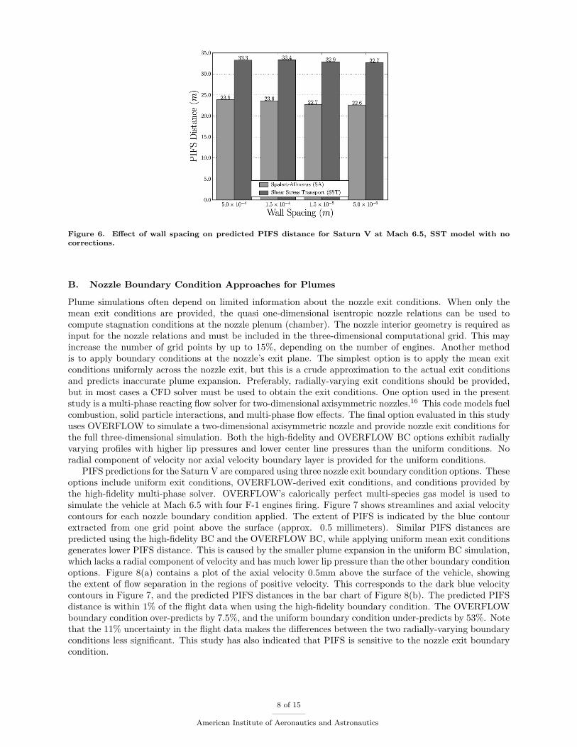
Figure 6. Effect of wall spacing on predicted PIFS distance for Saturn V at Mach 6.5, SST model with no
corrections.
B. Nozzle Boundary Condition Approaches for Plumes
Plume simulations often depend on limited information about the nozzle exit conditions. When only themean exit conditions are provided, the quasi one-dimensional isentropic nozzle relations can be used tocompute stagnation conditions at the nozzle plenum (chamber). The nozzle interior geometry is required asinput for the nozzle relations and must be included in the three-dimensional computational grid. This mayincrease the number of grid points by up to 15%, depending on the number of engines. Another methodis to apply boundary conditions at the nozzle’s exit plane. The simplest option is to apply the mean exitconditions uniformly across the nozzle exit, but this is a crude approximation to the actual exit conditionsand predicts inaccurate plume expansion. Preferably, radially-varying exit conditions should be provided,but in most cases a CFD solver must be used to obtain the exit conditions. One option used in the presentstudy is a multi-phase reacting flow solver for two-dimensional axisymmetric nozzles.16 This code models fuelcombustion, solid particle interactions, and multi-phase flow effects. The final option evaluated in this studyuses OVERFLOW to simulate a two-dimensional axisymmetric nozzle and provide nozzle exit conditions forthe full three-dimensional simulation. Both the high-fidelity and OVERFLOW BC options exhibit radiallyvarying profiles with higher lip pressures and lower center line pressures than the uniform conditions. Noradial component of velocity nor axial velocity boundary layer is provided for the uniform conditions.
PIFS predictions for the Saturn V are compared using three nozzle exit boundary condition options. Theseoptions include uniform exit conditions, OVERFLOW-derived exit conditions, and conditions provided bythe high-fidelity multi-phase solver. OVERFLOW’s calorically perfect multi-species gas model is used tosimulate the vehicle at Mach 6.5 with four F-1 engines firing. Figure 7 shows streamlines and axial velocitycontours for each nozzle boundary condition applied. The extent of PIFS is indicated by the blue contourextracted from one grid point above the surface (approx. 0.5 millimeters). Similar PIFS distances arepredicted using the high-fidelity BC and the OVERFLOW BC, while applying uniform mean exit conditionsgenerates lower PIFS distance. This is caused by the smaller plume expansion in the uniform BC simulation,which lacks a radial component of velocity and has much lower lip pressure than the other boundary conditionoptions. Figure 8(a) contains a plot of the axial velocity 0.5mm above the surface of the vehicle, showingthe extent of flow separation in the regions of positive velocity. This corresponds to the dark blue velocitycontours in Figure 7, and the predicted PIFS distances in the bar chart of Figure 8(b). The predicted PIFSdistance is within 1% of the flight data when using the high-fidelity boundary condition. The OVERFLOWboundary condition over-predicts by 7.5%, and the uniform boundary condition under-predicts by 53%. Notethat the 11% uncertainty in the flight data makes the differences between the two radially-varying boundaryconditions less significant. This study has also indicated that PIFS is sensitive to the nozzle exit boundarycondition.
8 of 15
American Institute of Aeronautics and Astronautics
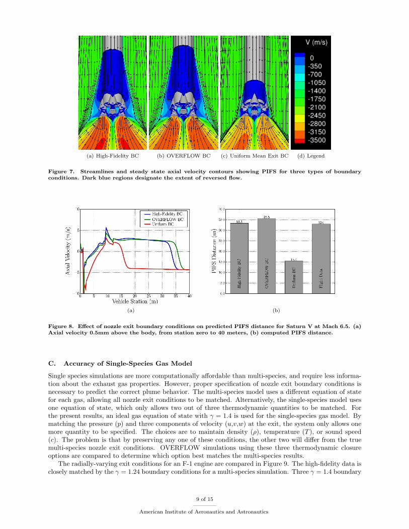
(a) High-Fidelity BC (b) OVERFLOW BC (c) Uniform Mean Exit BC (d) Legend
Figure 7. Streamlines and steady state axial velocity contours showing PIFS for three types of boundary
conditions. Dark blue regions designate the extent of reversed flow.
(a) (b)
Figure 8. Effect of nozzle exit boundary conditions on predicted PIFS distance for Saturn V at Mach 6.5. (a)
Axial velocity 0.5mm above the body, from station zero to 40 meters, (b) computed PIFS distance.
C. Accuracy of Single-Species Gas Model
Single species simulations are more computationally affordable than multi-species, and require less informa-tion about the exhaust gas properties. However, proper specification of nozzle exit boundary conditions isnecessary to predict the correct plume behavior. The multi-species model uses a different equation of statefor each gas, allowing all nozzle exit conditions to be matched. Alternatively, the single-species model usesone equation of state, which only allows two out of three thermodynamic quantities to be matched. Forthe present results, an ideal gas equation of state with γ = 1.4 is used for the single-species gas model. Bymatching the pressure (p) and three components of velocity (u,v,w) at the exit, the system only allows onemore quantity to be specified. The choices are to maintain density (ρ), temperature (T ), or sound speed(c). The problem is that by preserving any one of these conditions, the other two will differ from the truemulti-species nozzle exit conditions. OVERFLOW simulations using these three thermodynamic closureoptions are compared to determine which option best matches the multi-species results.
The radially-varying exit conditions for an F-1 engine are compared in Figure 9. The high-fidelity data isclosely matched by the γ = 1.24 boundary conditions for a multi-species simulation. Three γ = 1.4 boundary
9 of 15
American Institute of Aeronautics and Astronautics
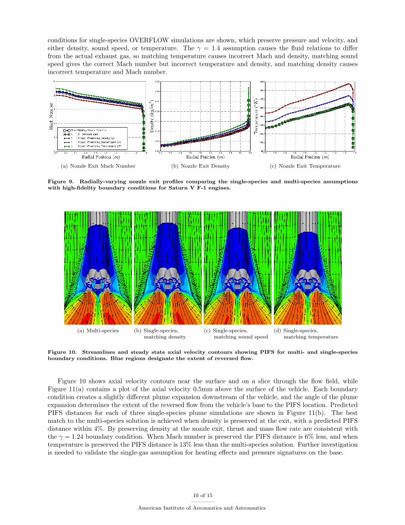
conditions for single-species OVERFLOW simulations are shown, which preserve pressure and velocity, andeither density, sound speed, or temperature. The γ = 1.4 assumption causes the fluid relations to differfrom the actual exhaust gas, so matching temperature causes incorrect Mach and density, matching soundspeed gives the correct Mach number but incorrect temperature and density, and matching density causesincorrect temperature and Mach number.
(a) Nozzle Exit Mach Number (b) Nozzle Exit Density (c) Nozzle Exit Temperature
Figure 9. Radially-varying nozzle exit profiles comparing the single-species and multi-species assumptions
with high-fidelity boundary conditions for Saturn V F-1 engines.
(a) Multi-species (b) Single-species,matching density
(c) Single-species,matching sound speed
(d) Single-species,matching temperature
Figure 10. Streamlines and steady state axial velocity contours showing PIFS for multi- and single-species
boundary conditions. Blue regions designate the extent of reversed flow.
Figure 10 shows axial velocity contours near the surface and on a slice through the flow field, whileFigure 11(a) contains a plot of the axial velocity 0.5mm above the surface of the vehicle. Each boundarycondition creates a slightly different plume expansion downstream of the vehicle, and the angle of the plumeexpansion determines the extent of the reversed flow from the vehicle’s base to the PIFS location. PredictedPIFS distances for each of three single-species plume simulations are shown in Figure 11(b). The bestmatch to the multi-species solution is achieved when density is preserved at the exit, with a predicted PIFSdistance within 4%. By preserving density at the nozzle exit, thrust and mass flow rate are consistent withthe γ = 1.24 boundary condition. When Mach number is preserved the PIFS distance is 6% less, and whentemperature is preserved the PIFS distance is 13% less than the multi-species solution. Further investigationis needed to validate the single-gas assumption for heating effects and pressure signatures on the base.
10 of 15
American Institute of Aeronautics and Astronautics
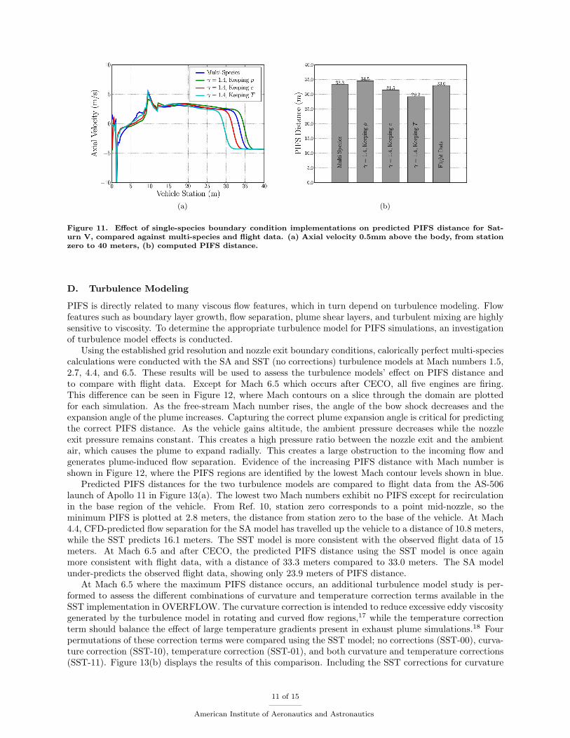
(a) (b)
Figure 11. Effect of single-species boundary condition implementations on predicted PIFS distance for Sat-
urn V, compared against multi-species and flight data. (a) Axial velocity 0.5mm above the body, from station
zero to 40 meters, (b) computed PIFS distance.
D. Turbulence Modeling
PIFS is directly related to many viscous flow features, which in turn depend on turbulence modeling. Flowfeatures such as boundary layer growth, flow separation, plume shear layers, and turbulent mixing are highlysensitive to viscosity. To determine the appropriate turbulence model for PIFS simulations, an investigationof turbulence model effects is conducted.
Using the established grid resolution and nozzle exit boundary conditions, calorically perfect multi-speciescalculations were conducted with the SA and SST (no corrections) turbulence models at Mach numbers 1.5,2.7, 4.4, and 6.5. These results will be used to assess the turbulence models’ effect on PIFS distance andto compare with flight data. Except for Mach 6.5 which occurs after CECO, all five engines are firing.This difference can be seen in Figure 12, where Mach contours on a slice through the domain are plottedfor each simulation. As the free-stream Mach number rises, the angle of the bow shock decreases and theexpansion angle of the plume increases. Capturing the correct plume expansion angle is critical for predictingthe correct PIFS distance. As the vehicle gains altitude, the ambient pressure decreases while the nozzleexit pressure remains constant. This creates a high pressure ratio between the nozzle exit and the ambientair, which causes the plume to expand radially. This creates a large obstruction to the incoming flow andgenerates plume-induced flow separation. Evidence of the increasing PIFS distance with Mach number isshown in Figure 12, where the PIFS regions are identified by the lowest Mach contour levels shown in blue.
Predicted PIFS distances for the two turbulence models are compared to flight data from the AS-506launch of Apollo 11 in Figure 13(a). The lowest two Mach numbers exhibit no PIFS except for recirculationin the base region of the vehicle. From Ref. 10, station zero corresponds to a point mid-nozzle, so theminimum PIFS is plotted at 2.8 meters, the distance from station zero to the base of the vehicle. At Mach4.4, CFD-predicted flow separation for the SA model has travelled up the vehicle to a distance of 10.8 meters,while the SST predicts 16.1 meters. The SST model is more consistent with the observed flight data of 15meters. At Mach 6.5 and after CECO, the predicted PIFS distance using the SST model is once againmore consistent with flight data, with a distance of 33.3 meters compared to 33.0 meters. The SA modelunder-predicts the observed flight data, showing only 23.9 meters of PIFS distance.
At Mach 6.5 where the maximum PIFS distance occurs, an additional turbulence model study is per-formed to assess the different combinations of curvature and temperature correction terms available in theSST implementation in OVERFLOW. The curvature correction is intended to reduce excessive eddy viscositygenerated by the turbulence model in rotating and curved flow regions,17 while the temperature correctionterm should balance the effect of large temperature gradients present in exhaust plume simulations.18 Fourpermutations of these correction terms were compared using the SST model; no corrections (SST-00), curva-ture correction (SST-10), temperature correction (SST-01), and both curvature and temperature corrections(SST-11). Figure 13(b) displays the results of this comparison. Including the SST corrections for curvature
11 of 15
American Institute of Aeronautics and Astronautics
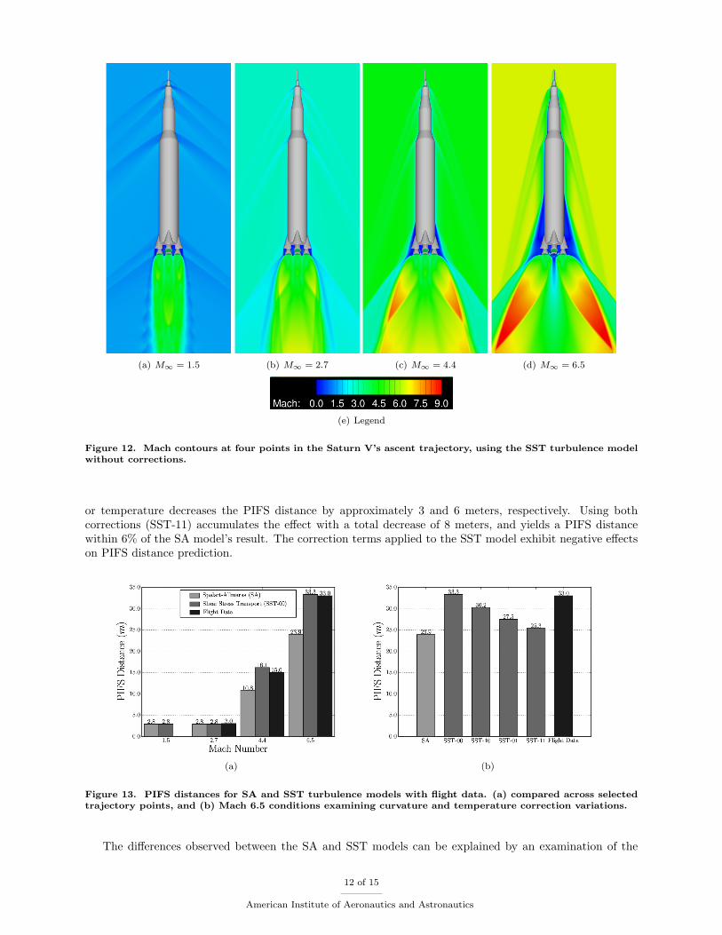
(a) M∞ = 1.5 (b) M∞ = 2.7 (c) M∞ = 4.4 (d) M∞ = 6.5
(e) Legend
Figure 12. Mach contours at four points in the Saturn V’s ascent trajectory, using the SST turbulence model
without corrections.
or temperature decreases the PIFS distance by approximately 3 and 6 meters, respectively. Using bothcorrections (SST-11) accumulates the effect with a total decrease of 8 meters, and yields a PIFS distancewithin 6% of the SA model’s result. The correction terms applied to the SST model exhibit negative effectson PIFS distance prediction.
(a) (b)
Figure 13. PIFS distances for SA and SST turbulence models with flight data. (a) compared across selected
trajectory points, and (b) Mach 6.5 conditions examining curvature and temperature correction variations.
The differences observed between the SA and SST models can be explained by an examination of the
12 of 15
American Institute of Aeronautics and Astronautics
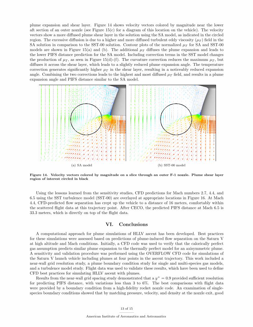
plume expansion and shear layer. Figure 14 shows velocity vectors colored by magnitude near the loweraft section of an outer nozzle (see Figure 15(c) for a diagram of this location on the vehicle). The velocityvectors show a more diffused plume shear layer in the solution using the SA model, as indicated in the circledregion. The excessive diffusion is due to a higher and more diffused turbulent eddy viscosity (µT ) field in theSA solution in comparison to the SST-00 solution. Contour plots of the normalized µT for SA and SST-00models are shown in Figure 15(a) and (b). The additional µT diffuses the plume expansion and leads tothe lower PIFS distance prediction for the SA model. Including correction terms in the SST model changesthe production of µT , as seen in Figure 15(d)-(f). The curvature correction reduces the maximum µT , butdiffuses it across the shear layer, which leads to a slightly reduced plume expansion angle. The temperaturecorrection generates significantly higher µT in the shear layer, resulting in a noticeably reduced expansionangle. Combining the two corrections leads to the highest and most diffused µT field, and results in a plumeexpansion angle and PIFS distance similar to the SA model.
(a) SA model (b) SST-00 model
Figure 14. Velocity vectors colored by magnitude on a slice through an outer F-1 nozzle. Plume shear layer
region of interest circled in black
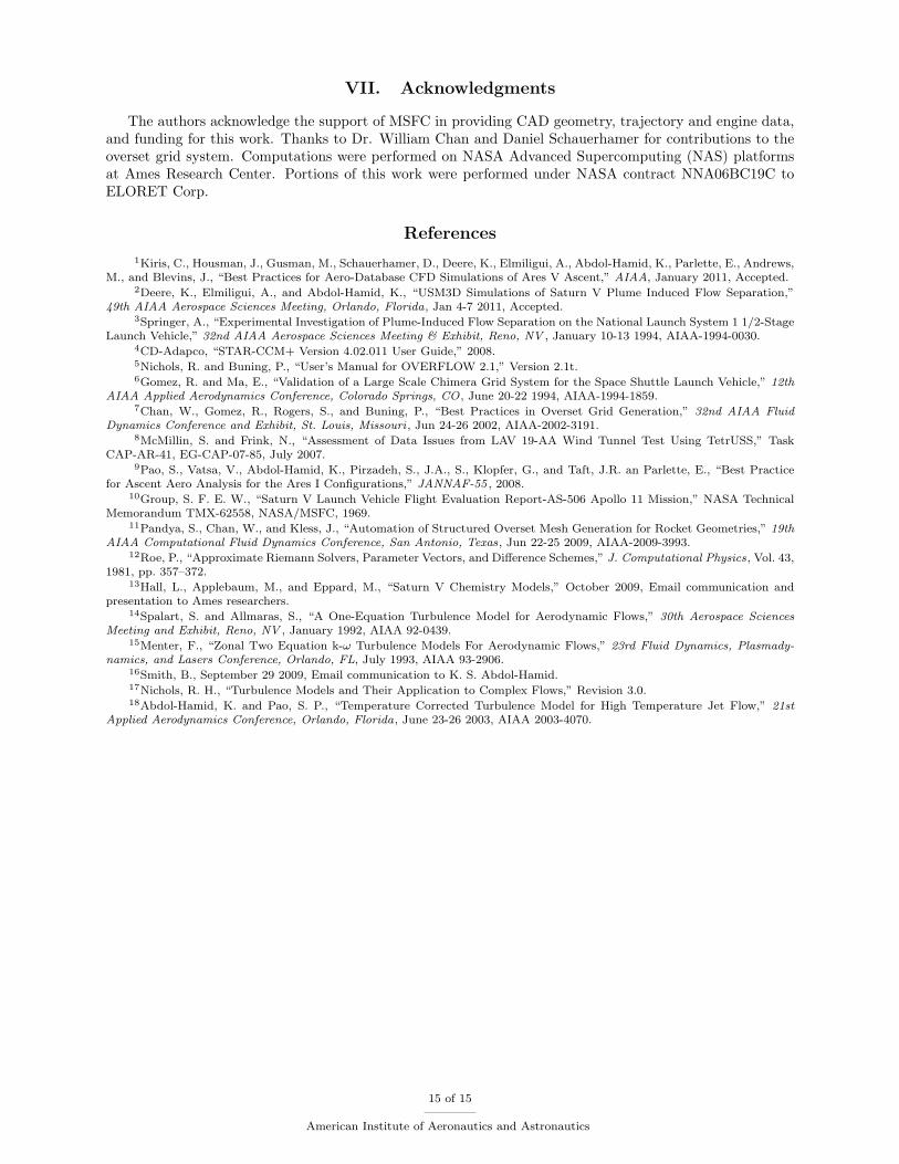
Using the lessons learned from the sensitivity studies, CFD predictions for Mach numbers 2.7, 4.4, and6.5 using the SST turbulence model (SST-00) are overlayed at appropriate locations in Figure 16. At Mach4.4, CFD-predicted flow separation has crept up the vehicle to a distance of 16 meters, comfortably withinthe scattered flight data at this trajectory point. After CECO, the predicted PIFS distance at Mach 6.5 is33.3 meters, which is directly on top of the flight data.
VI. Conclusions
A computational approach for plume simulations of HLLV ascent has been developed. Best practicesfor these simulations were assessed based on predictions of plume-induced flow separation on the Saturn Vat high altitude and Mach conditions. Initially, a CFD code was used to verify that the calorically perfectgas assumption predicts similar plume expansion to the thermally perfect model for an axisymmetric plume.A sensitivity and validation procedure was performed using the OVERFLOW CFD code for simulations ofthe Saturn V launch vehicle including plumes at four points in the ascent trajectory. This work included anear-wall grid resolution study, a plume boundary condition study for single and multi-species gas models,and a turbulence model study. Flight data was used to validate these results, which have been used to defineCFD best practices for simulating HLLV ascent with plumes.
Results from the near-wall grid spacing study demonstrated that a y+ = 0.9 provided sufficient resolutionfor predicting PIFS distance, with variations less than 3 to 6%. The best comparisons with flight datawere provided by a boundary condition from a high-fidelity rocket nozzle code. An examination of single-species boundary conditions showed that by matching pressure, velocity, and density at the nozzle exit, good
13 of 15
American Institute of Aeronautics and Astronautics
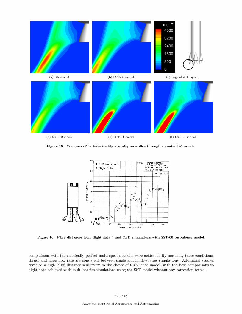
(a) SA model (b) SST-00 model (c) Legend & Diagram
(d) SST-10 model (e) SST-01 model (f) SST-11 model
Figure 15. Contours of turbulent eddy viscosity on a slice through an outer F-1 nozzle.
Figure 16. PIFS distances from flight data10 and CFD simulations with SST-00 turbulence model.
comparisons with the calorically perfect multi-species results were achieved. By matching these conditions,thrust and mass flow rate are consistent between single and multi-species simulations. Additional studiesrevealed a high PIFS distance sensitivity to the choice of turbulence model, with the best comparisons toflight data achieved with multi-species simulations using the SST model without any correction terms.
14 of 15
American Institute of Aeronautics and Astronautics
VII. Acknowledgments
The authors acknowledge the support of MSFC in providing CAD geometry, trajectory and engine data,and funding for this work. Thanks to Dr. William Chan and Daniel Schauerhamer for contributions to theoverset grid system. Computations were performed on NASA Advanced Supercomputing (NAS) platformsat Ames Research Center. Portions of this work were performed under NASA contract NNA06BC19C toELORET Corp.
References
1Kiris, C., Housman, J., Gusman, M., Schauerhamer, D., Deere, K., Elmiligui, A., Abdol-Hamid, K., Parlette, E., Andrews,M., and Blevins, J., “Best Practices for Aero-Database CFD Simulations of Ares V Ascent,” AIAA, January 2011, Accepted.
2Deere, K., Elmiligui, A., and Abdol-Hamid, K., “USM3D Simulations of Saturn V Plume Induced Flow Separation,”49th AIAA Aerospace Sciences Meeting, Orlando, Florida, Jan 4-7 2011, Accepted.
3Springer, A., “Experimental Investigation of Plume-Induced Flow Separation on the National Launch System 1 1/2-StageLaunch Vehicle,” 32nd AIAA Aerospace Sciences Meeting & Exhibit, Reno, NV , January 10-13 1994, AIAA-1994-0030.
4CD-Adapco, “STAR-CCM+ Version 4.02.011 User Guide,” 2008.5Nichols, R. and Buning, P., “User’s Manual for OVERFLOW 2.1,” Version 2.1t.6Gomez, R. and Ma, E., “Validation of a Large Scale Chimera Grid System for the Space Shuttle Launch Vehicle,” 12th
AIAA Applied Aerodynamics Conference, Colorado Springs, CO , June 20-22 1994, AIAA-1994-1859.7Chan, W., Gomez, R., Rogers, S., and Buning, P., “Best Practices in Overset Grid Generation,” 32nd AIAA Fluid
Dynamics Conference and Exhibit, St. Louis, Missouri , Jun 24-26 2002, AIAA-2002-3191.8McMillin, S. and Frink, N., “Assessment of Data Issues from LAV 19-AA Wind Tunnel Test Using TetrUSS,” Task
CAP-AR-41, EG-CAP-07-85, July 2007.9Pao, S., Vatsa, V., Abdol-Hamid, K., Pirzadeh, S., J.A., S., Klopfer, G., and Taft, J.R. an Parlette, E., “Best Practice
for Ascent Aero Analysis for the Ares I Configurations,” JANNAF-55 , 2008.10Group, S. F. E. W., “Saturn V Launch Vehicle Flight Evaluation Report-AS-506 Apollo 11 Mission,” NASA Technical
Memorandum TMX-62558, NASA/MSFC, 1969.11Pandya, S., Chan, W., and Kless, J., “Automation of Structured Overset Mesh Generation for Rocket Geometries,” 19th
AIAA Computational Fluid Dynamics Conference, San Antonio, Texas, Jun 22-25 2009, AIAA-2009-3993.12Roe, P., “Approximate Riemann Solvers, Parameter Vectors, and Difference Schemes,” J. Computational Physics, Vol. 43,
1981, pp. 357–372.13Hall, L., Applebaum, M., and Eppard, M., “Saturn V Chemistry Models,” October 2009, Email communication and
presentation to Ames researchers.14Spalart, S. and Allmaras, S., “A One-Equation Turbulence Model for Aerodynamic Flows,” 30th Aerospace Sciences
Meeting and Exhibit, Reno, NV , January 1992, AIAA 92-0439.15Menter, F., “Zonal Two Equation k-ω Turbulence Models For Aerodynamic Flows,” 23rd Fluid Dynamics, Plasmady-
namics, and Lasers Conference, Orlando, FL, July 1993, AIAA 93-2906.16Smith, B., September 29 2009, Email communication to K. S. Abdol-Hamid.17Nichols, R. H., “Turbulence Models and Their Application to Complex Flows,” Revision 3.0.18Abdol-Hamid, K. and Pao, S. P., “Temperature Corrected Turbulence Model for High Temperature Jet Flow,” 21st
Applied Aerodynamics Conference, Orlando, Florida, June 23-26 2003, AIAA 2003-4070.
15 of 15
American Institute of Aeronautics and Astronautics