CFD Modelling of a Two-Phase Closed Thermosyphon Charged with R134a and R404a

Bandar Fadhl a,+, Luiz C. Wrobel a*, Hussam Jouhara b a Institute of Materials and Manufacturing

b Institute of Energy Futures, RCUK Centre for Sustainable Energy Use in Food Chains (CSEF)

a,b College of Engineering, Design and Physical Sciences, Brunel University London, Uxbridge, Middlesex UB8 3PH, London, UK

Keywords: Two-phase thermosyphon, Computational fluid dynamics (CFD), Phase change material, Pool boiling, Liquid film condensation, R134a, R404a

1 A B S T R A C T

This paper examines the application of CFD modelling to simulate the two-phase heat

transfer mechanisms in a wickless heat pipe, also called a thermosyphon. Two

refrigerants, R134a and R404a, were selected as the working fluids of the

investigated thermosyphon. A CFD model was built to simulate the details of the

two-phase flow and heat transfer phenomena during the start-up and steady-state

operation of the thermosyphon. The CFD simulation results were compared with

experimental measurements, with good agreement obtained between predicted

temperature profiles and experimental temperature data, thus confirming that the CFD

model was successful in reproducing the heat and mass transfer processes in the

R134a and R404a charged thermosyphon, including the pool boiling in the evaporator

section and the liquid film in the condenser section.

+Permanent address: Department of Mechanical Engineering, Umm Al-Qura University, Makkah, KSA * Corresponding author. Tel.: +441895266696. E-mail address: luiz.wrobel@brunel.ac.uk

Page

2

2 INTRODUCTION

A wickless heat pipe is a two-phase heat transfer device with a highly effective

thermal conductivity, containing a small amount of working fluid that circulates in a

sealed tube utilising the gravity forces to return the condensate back to the evaporator

[1]. When the evaporator section is heated by an external source, the heat will be

transferred to the working fluid through the evaporator wall. The working fluid

absorbs an amount of heat proportional to the latent heat of evaporation, which is

sufficient to change the fluid from liquid to vapour. The vapour then moves to the

condenser section where it changes phase again, back to liquid, along the condenser's

wall, giving up its latent heat that it absorbed in the evaporator section. The

condensed liquid is then returned to the evaporator due to gravitational or capillary

forces, according to the type of heat pipe [1-5]. Heat pipes have been successfully

used for waste heat energy recovery in a vast range of engineering applications, such

as heating, ventilation, and air conditioning (HVAC) systems [2], ground source heat

pumps [6], water heating systems [7] and electronics thermal management [8].

The most important characteristics to consider in identifying suitable working fluids

are compatibility and wettability with the heat pipe materials, good thermal stability

and conductivity, high latent heat of evaporation, high surface tension and low

viscosity for both liquid and vapour [9]. In typical thermosyphons, the selection of the

working fluid and the shell materials is subject to the working environment and

temperature under which the thermosyphon-based system will function. For low

temperature applications, ammonia and various refrigerants such as R134a, R22 and

R410a have been used as working fluids with copper, steel, aluminium and other

compatible metals as shell materials. Water has been proven to be a suitable working

fluid for temperatures between 30°C and 300°C, with good compatibility with various

metals including copper and stainless steel. Liquid metals and various organic fluids

have been selected for thermosyphons when the working temperature is above 300°C

[6, 10-14].

Two-phase closed thermosyphons have been extensively used in many applications

[15]; however, only a limited number of CFD numerical simulation studies have been

published. Kafeel and Turan [16] studied the effect of different pulsed increases in

Page

3

heat input at the evaporator zone on the behaviour of thermosyphons. They used

similar thermosyphon configurations to that of Amatachaya et al [17] to validate the

simulation model, and an Eulerian model to simulate film condensation at the

condenser zone with a filling ratio of 30% of the evaporator zone. Alizadehdakhel et

al. [18] reported on a two-dimensional model and experimental studies in which they

investigated the effect of input heat flow and filling ratio of the working fluid on the

performance of a two-phase closed thermosyphon, using water as the working fluid.

Zhang et al. [19] developed a two-dimensional model for a disk-shaped flat two-

phase thermosyphon used in electronics cooling. The authors simulated the flow

inside the disk flat two-phase thermosyphon as a single-phase flow with water as the

working fluid. They compared the distribution of vapour velocity and temperature

with experimental results to determine the factors that affected the axial thermal

resistance of a flat thermosyphon.

Annamalai and Ramalingam [20] carried out an experimental investigation and CFD

analysis of a wicked heat pipe using ANSYS CFX. The authors considered the region

inside the heat pipe as a single phase of vapour and the wick region as the liquid

phase, and used distilled water as the working fluid. They compared the predicted

surface temperature along the evaporator and condenser walls and the vapour

temperature inside the heat pipe with the experimental data. Lin et al. [21] built a

CFD model to predict the heat transfer capability of miniature oscillating heat pipes

(MOHPs) using VOF and Mixture models, and water as the working fluid. The

effects of different heat transfer lengths and inner diameters at different heat inputs

were used to analyse the heat transfer capability of MOHPs.

There is an obvious gap in the published literature on CFD simulations of the two-

phase heat transfer/flow within a wickless heat pipe. Therefore, the purpose of this

paper is to build a CFD model to cover all details of two-phase flow and heat transfer

phenomena during the operation of a wickless heat pipe charged with two working

fluids, namely R134a and R404a. The reported work focuses on their thermal

performance during start-up and operation. The developed CFD model has been

validated experimentally and theoretically with good agreement. A user-defined

Page

4

function (UDF), together with a VOF model, has been used in order to simulate the

phase change during the pool boiling and the liquid film condensation.

3 CFD SIMULATION OF MASS AND HEAT TRANSFER DURING THE EVAPORATION AND CONDENSATION PROCESSES

In this study, the commercial code ANSYS FLUENT 14.0 and the Volume of Fluid

(VOF) method have been applied for the modelling of a closed two-phase

thermosyphon. The details of the VOF model and the Navier-Stokes equations for the

VOF model, relevant to this study, have been discussed by Fadhl et al. [1].

During the thermosyphon operation, phase change occurs from liquid to vapour phase

during the nucleate pool boiling in the evaporator section and from vapour to liquid

phase during the liquid film condensation in the condenser section. In this study, user-

defined functions (UDFs) are employed to specify customised source terms reported

by Fadhl et al. [1] and De Schepper et al. [22] for the existing governing equations in

the FLUENT package, in order to determine mass and energy sources for the phases

involved in the mass and heat transfer processes.

Mass sources, SM in the volume fraction equation, can be given by the following

expressions:

For mass transfer during the evaporation process:

sat

satmixLLM T

TTS −−= aρ1.0

1 (1)

( )12 MM SS −= (2)

For mass transfer during the condensation process:

sat

mixsatVVM T

TTS −= aρ1.0

3 (3)

( )34 MM SS −= (4)

where Tmix and Tsat are the mixture and saturation temperatures, respectively, and 𝛼𝛼𝐿𝐿

and 𝛼𝛼𝑉𝑉 are the volume fraction of the liquid and vapour phases, respectively.

Page

5

In the VOF model, the temperature is introduced as a mixture temperature rather than

liquid or vapour temperatures, as the VOF model associates some variables such as

temperature and velocity with the mixture phase, not with a specific phase. The

volume fraction for each phase in the cell has been defined by the VOF model.

Therefore, the evaporation process required two mass sources for the calculation of

the mass transfer, Eq. (1) describing the amount of mass taken from the liquid phase

and Eq. (2) describing the amount of mass added to the vapour phase. The same

procedure takes place for the condensation process, Eq. (3) and Eq. (4) describing the

amount of mass transfer from vapour to liquid phase.

Energy sources SE in the energy equation used in the present study are determined by

multiplying the calculated mass sources in Eq. (1) and Eq. (3) by the latent heat of

evaporation for the working fluid, and can be expressed as follows;

( )LHSS ME .11

= (5)

( )LHSS ME .32

= (6)

where LH is latent heat of evaporation. A single source term for both phases is

required in the evaporation, Eq. (5) or condensation, Eq. (6) during the heat transfer

process.

4 MODEL GEOMETRY AND COMPUTATIONAL MESH

A two-dimensional model was developed to simulate the two-phase flow and heat

transfer phenomena in a thermosyphon. According to the experimental conditions

described in [1], a closed thermosyphon tube wall made of copper with a thickness of

0.9mm and a total length of 500mm was used as the thermosyphon geometry, as can

be seen in Figure 1. The evaporator and condenser sections of the thermosyphon

model are taken to be 200mm in length, making the adiabatic section 100mm long.

The outer and inner diameters are 22mm and 20.2mm, respectively.

The temperature distribution along the thermosyphon wall was monitored using eight

thermocouples, according to the experimental setup [1]. As shown in Figure 1, Ta

gave the temperature of the adiabatic section, Te1 and Te2 were used to obtain the

Page

6

average temperature of the evaporator section, while Tc1 to Tc5 were used to for the

average temperature of the condenser section.

The geometry was constructed and meshed using the GAMBIT grid generation

software. The solid and fluid regions contain 24,944 and 105,000 Quad cells,

respectively. Near the left and right walls, fifteen layers of cells are used in order to

capture the thin liquid film that develops in that region. The first grid size is 0.01mm

and the growth ratio is 1.2. Three layers of 180 cells have been used for the upper and

bottom walls. Boundary conditions on the upper and lower caps of the thermosyphon

are set to adiabatic, as shown in Figure 2.

Different mesh sizes were used to test grid independence as shown in Figure 3. The

average temperature of the evaporator (Tevaporator), adiabatic (Tadiabatic) and condenser

(Tcondenser) sections for different mesh sizes for the R134a working fluid were

monitored and are shown in Table 1. For the R134a-charged thermosyphon and

heating power of 30 W, it was found that almost the same average temperatures for

the evaporator, adiabatic and condenser sections were obtained for different mesh

sizes. As a result, the mesh size of 129,944 Quad cells, Map cells is selected for the

simulation analysis.

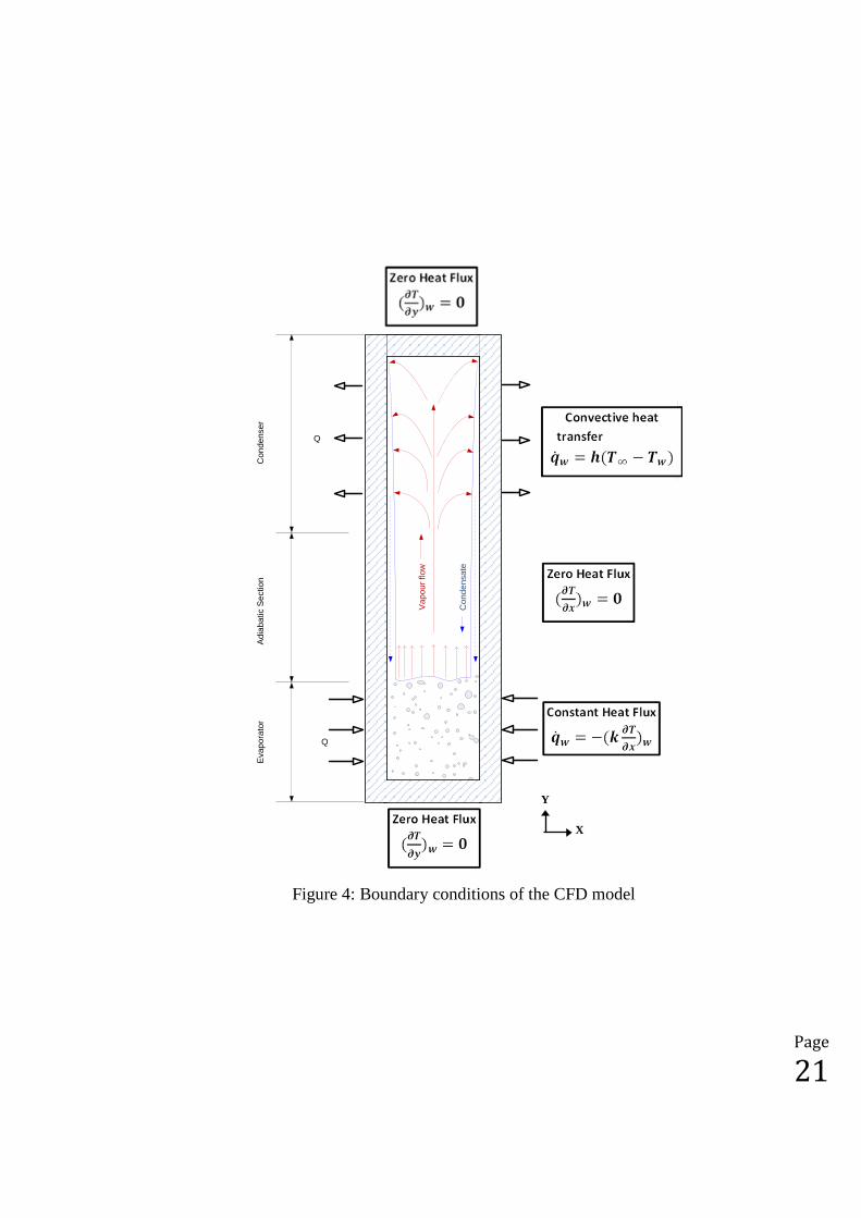
5 BOUNDARY AND OPERATING CONDITIONS

A non-slip boundary condition was imposed at the inner walls of the thermosyphon.

In order to simulate the heating and evaporation, a constant heat flux was defined at

the wall boundaries of the evaporator section, depending on the power input. A zero

heat flux is defined as boundary condition on the adiabatic section. The condenser

section was cooled as a result of heat released when vapour condenses. It has been

assumed that the condenser is cooled by water, according to the experimental

apparatus. Thus, a convection heat transfer coefficient was defined as boundary

condition on the condenser’s wall. The corresponding heat transfer coefficients have

been calculated using the formula:

( )∞−=

TTrLQh

avcc

cc

,2π (7)

Page

7

where hc is the condenser heat transfer coefficient, Qc is the rate of heat transfer from

the condenser, Lc is the condenser height, r is the pipe radius, Tc,av is the condenser

average temperature and T∞ is the average temperature of the condenser cooling

water. Figure 4 illustrates the boundary conditions implemented to the computational

model.

In order to verify the sensitivity of the results to the value of the heat transfer

coefficients, an empirical correlation proposed by Zukauskas [23] is used to

determine the average Nusselt number for external forced convection over a circular

pipe, defined as:

𝑁𝑁𝑁𝑁𝑍𝑍𝑍𝑍𝑍𝑍𝑍𝑍𝑍𝑍𝑍𝑍𝑍𝑍𝑍𝑍𝑍𝑍 = ℎ𝑐𝑐 𝑥𝑥 𝐷𝐷𝑐𝑐𝑍𝑍𝑙𝑙

= 0.683 𝑅𝑅𝑅𝑅0.466 𝑃𝑃𝑃𝑃𝑙𝑙13 (for 40 ≤ Re ≥ 4000) (8)

𝑅𝑅𝑅𝑅 =𝑈𝑈 𝑥𝑥 𝐷𝐷𝑐𝑐𝑣𝑣𝑙𝑙

(9)

where 𝑘𝑘𝑙𝑙, 𝑣𝑣𝑙𝑙 and 𝑃𝑃𝑃𝑃𝑙𝑙 are the thermal conductivity, kinematic viscosity and Prandtl

number of the condenser cooling water, U is the inlet cooling water velocity and Dc is

the condenser outer diameter.

Churchill and Bernstein [24] reported an additional correlation to determine the

average Nusselt number, defined as:

𝑁𝑁𝑁𝑁𝐶𝐶ℎ𝑍𝑍𝑢𝑢𝑐𝑐ℎ𝑖𝑖𝑙𝑙𝑙𝑙 = ℎ𝑐𝑐 𝑥𝑥 𝐷𝐷𝑐𝑐𝑍𝑍𝑙𝑙

= 0.3 + 𝑅𝑅𝑅𝑅0.5 𝑃𝑃𝑢𝑢13

[1+(0.4/𝑃𝑃𝑟𝑟)23]14�1 + � 𝑅𝑅𝑅𝑅

282,000�58�

45

(0.62) (10)

In order to test the simulation results independence on the condenser heat transfer

coefficients, correlations (7), (8) and (10) were checked for the heating power

throughput of 30 W for the working fluid R134a. Thus, the average temperature of

the evaporator, adiabatic and condenser sections are shown in Table 2. From this

observation, it is apparent that the average temperature for the evaporator, adiabatic

and condenser are very close for different tested correlations. Consequently,

correlation (7) is selected to determine the heat transfer coefficients of the condenser's

wall based on the experimental data (see Table 3).

Page

8

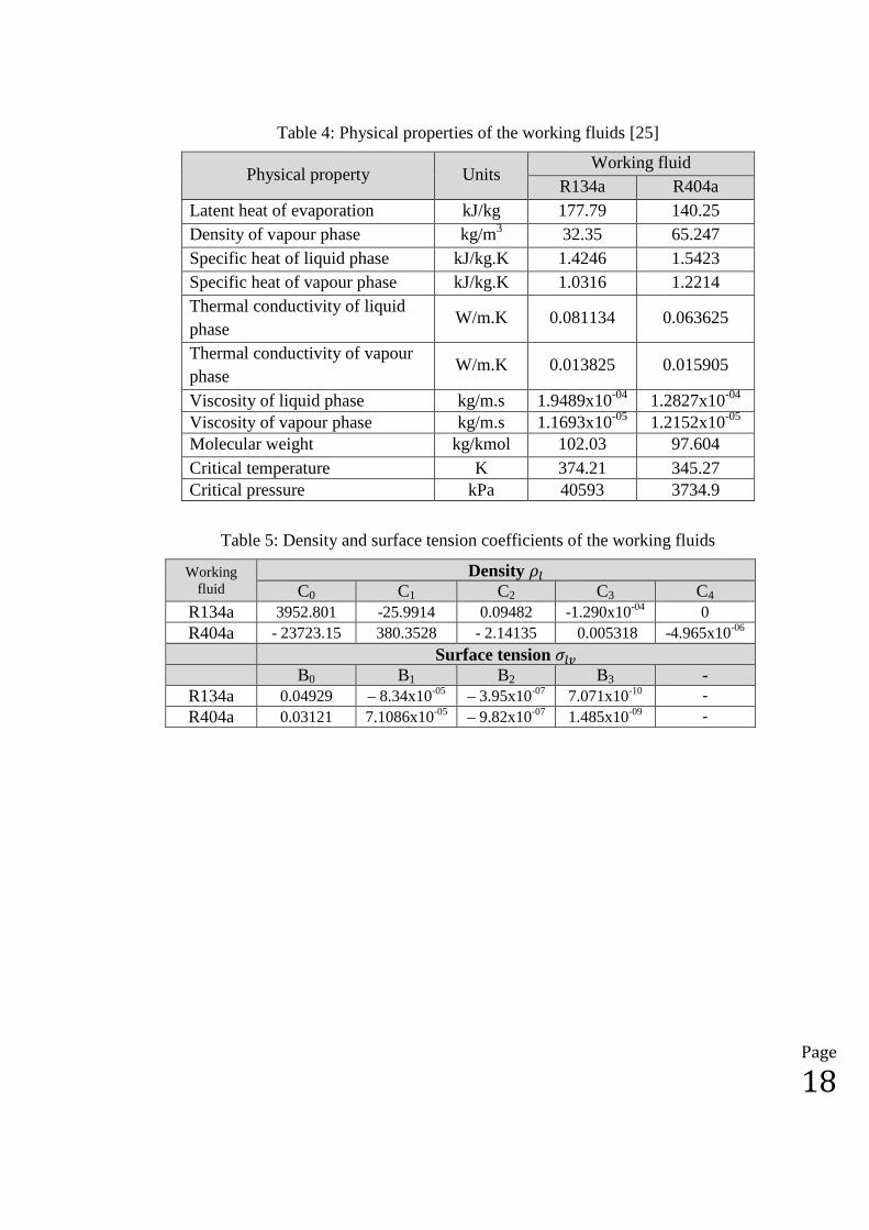
The model considered R134a or R404 as working fluids with a 100% filling ratio of

the evaporator section (i.e. FR=100%). Apart from the density of the liquid phase and

surface tension, the physical properties of the working fluids are assumed to be

temperature-independent to limit the calculation time. These properties are taken at

298.15 K using the NIST REFPROP program [25], and can be found in Table 4.

The density of the liquid phase (𝜌𝜌𝑙𝑙) of the working fluid is considered as temperature-

dependent and fitted into functions of temperature in the form of a high-order

polynomial, defined as:

𝜌𝜌𝑙𝑙(𝑇𝑇) = �𝐶𝐶𝑖𝑖 . 𝑇𝑇𝑖𝑖𝑛𝑛=4

𝑖𝑖=0

(11)

where 𝐶𝐶𝑖𝑖 are the density coefficients listed in Table 5.

The effect of surface tension (𝜎𝜎𝑙𝑙𝑙𝑙) along the interface between the two phases is also

considered as temperature-dependent and included in the model by using the

following correlation.

𝜎𝜎𝑙𝑙𝑙𝑙(𝑇𝑇) = �𝐵𝐵𝑖𝑖 . 𝑇𝑇𝑖𝑖𝑛𝑛=3

𝑖𝑖=0

(12)

where 𝐵𝐵𝑖𝑖 are the surface tension coefficients listed in Table 5.

The thermophysical properties listed in tables 4 & 5 have been obtained from the

NIST REFPROP program [25].

6 CFD SOLUTION PROCEDURE

A transient simulation with a time step of 0.001s is carried out to model the dynamic

behaviour of the two-phase flow. The time step has been selected based on the

Courant number, which is the ratio of the time step to the time a fluid takes to move

across a cell. For VOF models, the maximum Courant number allowed near the

interface is 250 [21]. For a time step of 0.001, the Courant number is less than 1. The

simulation reaches a steady state within 120s.

Page

9

FLUENT provides different segregated algorithms for pressure-velocity coupling. For

reduced CPU time and to avoid convergence difficulties, a combination of the

SIMPLE algorithm for pressure-velocity coupling and a first-order upwind scheme

for the determination of momentum and energy is included in the model. Geo-

Reconstruct and PRESTO discretization for the volume fraction and pressure

interpolation scheme, respectively, are also performed in the simulation. In the

current work, the numerical computation is considered to have converged when the

scaled residual was 10-5 for the mass and velocity components and about 10-6 for the

energy component.

The vapour phase of the working fluid is defined as the primary phase and the liquid

phase is defined as the secondary phase. For the calculation of the mass and heat

transfer during the evaporation and condensation processes, the boiling temperatures

and the latent heat of evaporation of the working fluids have been defined in the UDF

code. When the simulation was started, the liquid pool in the evaporator is heated

first. Once the saturation temperature defined in the UDF is reached, evaporation

starts and phase change occurs due to boiling at the inner evaporator wall. The

saturated vapour then flows upward, where it condenses along the inner cold walls of

the condenser forming a thin liquid film.

7 FLOW VISUALISATION OF CFD SIMULATION

In the following sub-sections, the CFD simulation findings from the tests will be

visualised and an analysis of the nature of the heat transfer, pool boiling and liquid

film condensation processes within the R134a and R404a charged thermosyphons

will be discussed.

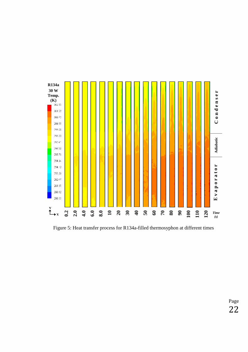
7.1 Heat transfer process

In order to understand the heat transfer process during the thermosyphon operation,

the temperature contours at different times have been observed during the start-up

(heating) and steady-state operation. In this visual observation, the temperature

distribution in the fluid region inside the evaporator, adiabatic and condenser sections

has been recorded for both R134a and R404a. The results for R134a are shown in

Page

10

Figure 5. A heating power of 30 W was selected to compare the heat transfer process

for both working fluids.

At the beginning of the heating procedure, the operating pressure and temperature of

the working fluid were set to the saturation values at the initial temperature of the

heat pipe (around 25°C for both cases), as shown in Figure 5. Between 2.0 s and 8.0

s, the temperature in the evaporator increases as a constant heat is applied to the outer

wall of the evaporator section, which allows heat to transfer through the evaporator

wall into the liquid pool, as shown in Figure 5. Boiling heat transfer continues on the

walls of the evaporator section due to the temperature difference between the wall

and the saturated working fluid within the thermosyphon. The generated vapour then

moves upward, as shown at 20 s, and this vapour flows through the adiabatic section

to the condenser section, as can be seen at 30 s, 40 s and 50 s in Figure 5. Then, a

high temperature region appears in the condenser section between 60 s and 90 s due

to the vapour reaching this section. The region near the inner wall of the condenser

section has a lower temperature than the middle region as a result of vapour

condensing along the inner surface of the condenser wall. Eventually, between 100 s

and 120 s, the temperature distribution inside the thermosyphon becomes uniform as

shown in Figure 5. The above described procedure shows the heat transfer process

during the operation of the thermosyphon charged with R134a. The same can be

observed for the case when the thermosyphon was charged with R404a.

Consequently, the temperature distribution in the fluid region inside the

thermosyphon for R404a has not been shown.

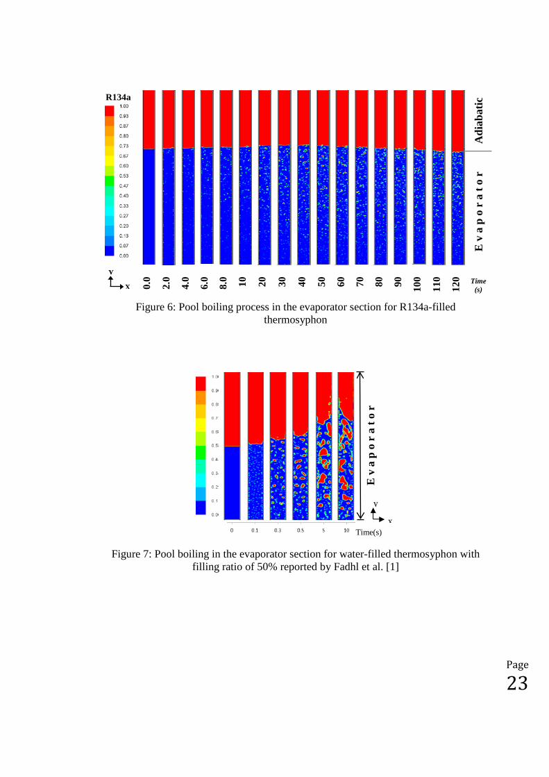
7.2 Evaporation process

The pool boiling phenomena taking place inside the evaporator section has also been

visualised during the evaporation process. Figure 6 shows the volume fraction

contours of the liquid pool in the evaporator section for R134a, for a power

throughput of 30 W. The liquid pool of the tested working fluid is represented by a

blue colour, which takes the value of 0 for the vapour volume fraction, and the vapour

is represented by a red colour, which takes the value of 1 for the vapour volume

fraction.

Page

11

The working fluids have initially filled the total volume of the evaporator section, as

shown in Figure 6 at 0.0 s. By applying a constant heat flux onto the wall of the

evaporator section, heat is then conducted through the evaporator wall to the inner

wall to be transferred into the saturated liquid by boiling. Due to the weight of the

working fluid column, localised natural convection currents at the lower half of the

evaporator section can be seen due to the slight increase in the saturation

pressure/temperature of the working fluid. The liquid starts to boil at a position where

the liquid temperature at the wall exceeds the saturation temperature (at the adjacent

liquid film that is stuck on the inner wall of the evaporator), hence local nucleation

sites critical radiuses are exceeded so continuous nucleation takes place. Vapour

bubbles then start to form at those positions, as shown in Figure 6 between 2.0 s and

10 s. By continuous nucleation, isolated vapour bubbles form and rise all the way up

to the top region of the liquid pool before breaking up and releasing their vapour

content. This is illustrated in Figure 6 at time 20 s and above. During the evaporation

process described above, the liquid volume fraction decreases and the vapour volume

fraction increases. The same procedure has been obtained for R404a. Consequently,

the volume fraction contours of the liquid pool in the evaporator section for R404a

have not been shown.

It is clear from Figure 6 that the pool boiling behaviour of R134a is significantly

different to that of water, as very small bubbles grow during the pool boiling. The

reason behind this is related to the value of the critical nucleation site radiuses. Fadhl

et al [1] reported CFD simulations of the pool boiling behaviour of water with the

filling ratio of 50%, a snapshot of which can be seen in Figure 7. The results for both

water and the refrigerants have been validated visually using transparent glass

wickless heat pipes. This provides evidence that the CFD model has the ability to

reproduce the difference in pool boiling behaviour between different working fluids.

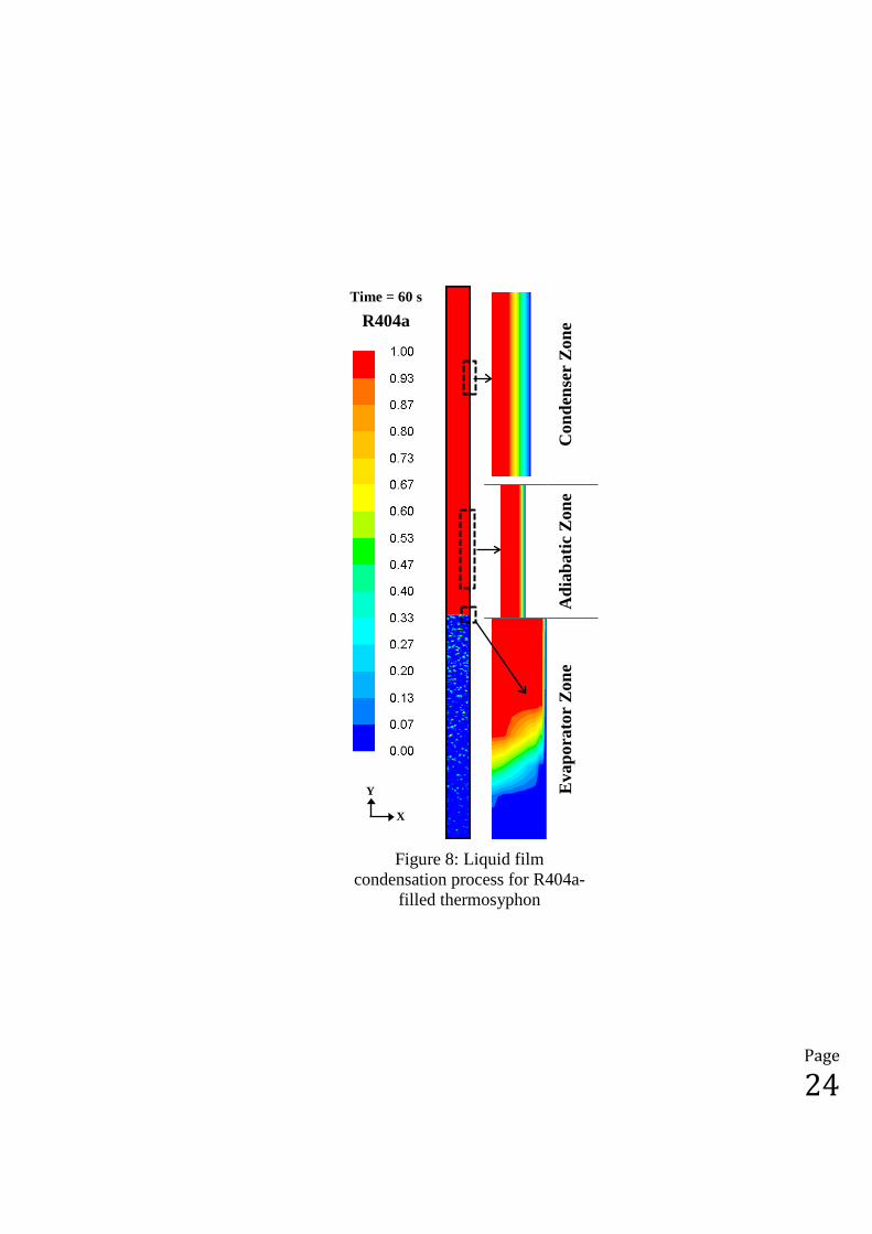
7.3 Condensation process

Following the boiling process, the converse process takes place in the condenser

section. The CFD model predicts the condensate film configuration as illustrated in

Page

12

Figure 8 for the R404a charged thermosyphon that was undergoing a power

throughput of 30 W.

It is illustrated that the liquid film will then fall down under gravity through the

adiabatic section, which is clearly shown in Figure 8 at the adiabatic zone.

Eventually, the liquid pool in the evaporator section will be charged by a continuous

thin liquid film as illustrated in Figure 8 at the evaporator zone.

8 TEMPERATURE DISTRIBUTION OF CFD SIMULATION OF THERMOSYPHON

The temperature profiles along the modelled thermosyphon have been observed under

different power throughputs using 8 positions in the model, which allowed the

monitoring of the average wall temperatures of the evaporator, adiabatic and

condenser sections. Two positions placed 40mm and 160mm from the bottom are

used to monitor the evaporator section and one position is used at the centre of the

adiabatic section. Five evenly spaced positions are used to monitor the condenser

section. These five positions are used to confirm the absence of non-condensable

gases which, if present, would be swept by the vapour towards the top area of the

condenser section where they would accumulate and reduce the thermal performance.

Thus, non-condensable gases are neglected in the current CFD model.

Figures 9 and 10 illustrate the experimental and CFD simulation temperature

distributions along the R134a and R404a charged thermosyphons, respectively, for

varying applied heat loads. The distance between 0 and 200mm indicates the

evaporator section, while the distance between 300 and 500mm indicates the

condenser section. The middle section is the adiabatic region. The CFD simulation

results of temperature distribution profiles have been compared with the experimental

data by determining the average relative error (ARE), which is the absolute

percentage difference between CFD simulation and experimental average wall

temperature. As depicted in Figures 9 and 10, the CFD simulation results showed the

same trend as the experimental results.

Page

13

Referring to Figures 9 and 10, the CFD simulation results of the selected

thermosyphon showed very good agreement with the temperature profiles from

experimental data for the lower power throughputs. The average wall temperatures of

the evaporator, adiabatic and condenser are close to those obtained in the

experiments. As a result, the ARE of evaporator, adiabatic and condenser average

wall temperatures are 1.25%, 0.78% and 1.03%, respectively for R134a, and 2.66%,

0.78% and 0.49%, respectively for R404a. For heat loads above approximately 60 W,

the predicted CFD evaporator average temperature has deviated from the

experimental results due to the consideration of a continuous heat power input along

the length of the evaporator section where, in the experiment, a wire heater is evenly

wrapped around the evaporator section to ensure it was not directly above a

thermocouple.

9 CONCLUSIONS

A two-phase closed thermosyphon is considered in this paper when charged with two

working fluids, R134a and R404a, in CFD simulations of the evaporation and

condensation phenomena inside the thermosyphon. The findings of the CFD

simulations demonstrate that the proposed CFD model can successfully reproduce the

complex phenomena inside the thermosyphon, including the pool boiling in the

evaporator section and the liquid film in the condenser section. The proposed CFD

model was validated solely with the limited experimental data available and further

validation is still necessary over greater operating ranges/configurations.

The CFD results show that the pool boiling behaviour of both refrigerants is

significantly different to that of water, as very small bubbles grow during the pool

boiling. The results for both water and the refrigerants have been validated by

visualisation experiments carried out with a transparent glass heat pipe. This provides

evidence that the CFD model has the ability to simulate thermosyphons charged with

different working fluids.

Page

14

The average wall temperature along the thermosyphon has been compared with the

experimental results at the same condition for both working fluids, and demonstrates

that the predicted CFD simulation results agreed with the experimental results.

Acknowledgment

The first author deeply appreciates the financial support in the form of a PhD

studentship offered by Mechanical Engineering Department, Umm Al-Qura

University, Ministry of Higher Education, Kingdom of Saudi Arabia.

10 REFERENCES

[1] Fadhl B, Wrobel LC, Jouhara H. Numerical modelling of the temperature distribution in a two-phase closed thermosyphon. Applied Thermal Engineering 2013; 60: 122-131.

[2] Kerrigan K, Jouhara H, O'Donnell GE, Robinson AJ. Heat pipe-based radiator for low grade geothermal energy conversion in domestic space heating. Simulation Modelling Practice and Theory 2011; 19: 1154-1163.

[3] ESDU. Heat pipes - general information on their use, operation and design. ESDU Manual 80013 1980.

[4] Faghri A. Heat Pipe Science and Technology. Taylor & Francis: Washington, D.C., 1995.

[5] Dunn P, Reay DA. Heat Pipes. Pergamon Press: New York, 1994;343.

[6] Jouhara H, Meskimmon R. Experimental investigation of wraparound loop heat pipe heat exchanger used in energy efficient air handling units. Energy 2010; 35: 4592-4599.

[7] Mathioulakis E, Belessiotis V. A new heat-pipe type solar domestic hot water system. Solar Energy 2002; 72: 13-20.

[8] Weng Y-, Cho H-, Chang C-, Chen S-. Heat pipe with PCM for electronic cooling. Applied Energy 2011; 88: 1825-1833.

[9] Reay D, Kew P. Heat Pipes: Theory, Design and Applications. Elsevier Science & Technology: UK, 2009;367.

Page

15

[10] Jouhara H, Robinson AJ. An experimental study of small-diameter wickless heat pipes operating in the temperature range 200oC to 450oC. Heat Transfer Engineering 2009; 30: 1041-1048.

[11] Groll M. Heat pipe research and development in western Europe. Heat Recovery Systems and CHP 1989; 9: 19-66.

[12] Abou-Ziyan HZ, Helali A, Fatouh M, Abo El-Nasr MM. Performance of stationary and vibrated thermosyphon working with water and R134a. Applied Thermal Engineering 2001; 21: 813-830.

[13] Ong KS, Haider-E-Alahi M. Performance of a R-134a-filled thermosyphon. Applied Thermal Engineering 2003; 23: 2373-2381.

[14] Yau YH, Foo YC. Comparative study on evaporator heat transfer characteristics of revolving heat pipes filled with R134a, R22 and R410A. International Communications in Heat and Mass Transfer 2011; 38: 202-211.

[15] Jiao B, Qiu LM, Zhang XB, Zhang Y. Investigation on the effect of filling ratio on the steady-state heat transfer performance of a vertical two-phase closed thermosyphon. Applied Thermal Engineering 2008; 28: 1417-1426.

[16] Kafeel K, Turan A. Simulation of the response of a thermosyphon under pulsed heat input conditions. International Journal of Thermal Sciences 2014; 80: 33-40.

[17] Amatachaya P, Srimuang W. Comparative heat transfer characteristics of a flat two-phase closed thermosyphon (FTPCT) and a conventional two-phase closed thermosyphon (CTPCT). International Communications in Heat and Mass Transfer 2010; 37: 293-298.

[18] Alizadehdakhel A, Rahimi M, Alsairafi AA. CFD modeling of flow and heat transfer in a thermosyphon. International Communications in Heat and Mass Transfer 2010; 37: 312-318.

[19] Zhang M, Liu Z, Ma G, Cheng S. Numerical simulation and experimental verification of a flat two-phase thermosyphon. Energy Conversion and Management 2009; 50: 1095-1100.

[20] Annamalai AS, Ramalingam V. Experimental investigation and computational fluid dynamics analysis of an air cooled condenser heat pipe. Thermal Science 2011; 15: 759-772.

[21] Lin Z, Wang S, Shirakashi R, Winston Zhang L. Simulation of a miniature oscillating heat pipe in bottom heating mode using CFD with unsteady modeling. International Journal of Heat and Mass Transfer 2013; 57: 642-656.

Page

16

[22] De Schepper SCK, Heynderickx GJ, Marin GB. Modeling the evaporation of a hydrocarbon feedstock in the convection section of a steam cracker. Computers & Chemical Engineering 2009; 33: 122-132.

[23] Žukauskas A. Heat Transfer from Tubes in Crossflow. Advances in Heat Transfer. Elsevier:93-160.

[24] Churchill SW, Bernstein M. Correlating equation for forced convection from gases and liquids to a circular cylinder in crossflow. Journal of Heat Transfer 1977; 99: 300-306.

[25] Lemmon EW, Huber ML, McLinden MD. NIST Standard Reference Database 23: Reference Fluid Thermodynamics and Transport Properties-REFPROP. National Institute of Standards and Technology, Standard Reference Data Program, Gaithersburg 2013; Version 9.1.

Page

17

TABLES

Table 1: Grid-independence results for thermosyphon charged with R134a

Mesh size (cells) 19,500 69,276 129,944 Tevaporator K 303.66 302.31 302.47 Tadiabatic K 299.18 299.01 299.64 Tcondenser K 294.63 294.80 295.62

Table 2: Average temperatures for the thermosyphon charged with R134a for different heat transfer coefficient correlations

Correlation of condenser heat transfer coefficient Eq. (7) Eq. (8) Eq. (10)

hc W/m2.K 394.4 592.3 654.6 Tevaporator K 302.47 302.29 302.22 Tadiabatic K 299.64 299.80 299.74 Tcondenser K 295.62 295.14 294.99

Table 3: Condenser heat transfer coefficients for different heat inputs R134a

Evaporator section

Condenser cooling water Jacket

Condenser section

Qin T∞ Qc Tc av hc W K W K W/m2.K

19.74 293.4 19.74 296.1 531.6 29.58 292.2 29.58 297.6 394.4 39.53 291.4 39.53 301.5 284.6 50.16 292.1 50.16 300.8 414.6 100.44 296.7 100.44 306.7 728.4

R404a 19.88 298.3 19.88 300.3 730.3 29.04 296.3 29.04 298.7 848.7 40.66 296.1 40.66 299.4 894.7 49.61 296.9 49.61 301 885.5 100.65 297.3 100.65 304.5 1008.7

Page

18

Table 4: Physical properties of the working fluids [25]

Physical property Units Working fluid

R134a R404a Latent heat of evaporation kJ/kg 177.79 140.25 Density of vapour phase kg/m3 32.35 65.247 Specific heat of liquid phase kJ/kg.K 1.4246 1.5423 Specific heat of vapour phase kJ/kg.K 1.0316 1.2214 Thermal conductivity of liquid phase

W/m.K 0.081134 0.063625

Thermal conductivity of vapour phase

W/m.K 0.013825 0.015905

Viscosity of liquid phase kg/m.s 1.9489x10-04 1.2827x10-04 Viscosity of vapour phase kg/m.s 1.1693x10-05 1.2152x10-05 Molecular weight kg/kmol 102.03 97.604 Critical temperature K 374.21 345.27 Critical pressure kPa 40593 3734.9

Table 5: Density and surface tension coefficients of the working fluids

Working fluid

Density 𝜌𝜌𝑙𝑙 C0 C1 C2 C3 C4

R134a 3952.801 -25.9914 0.09482 -1.290x10-04 0 R404a - 23723.15 380.3528 - 2.14135 0.005318 -4.965x10-06

Surface tension 𝜎𝜎𝑙𝑙𝑙𝑙 B0 B1 B2 B3 -

R134a 0.04929 – 8.34x10-05 – 3.95x10-07 7.071x10-10 - R404a 0.03121 7.1086x10-05 – 9.82x10-07 1.485x10-09 -

Page

19

FIGURES

Figure 1: Model geometry and dimension [1]

Te1

Te2

Ta

Tc1

Tc2

Tc3

Tc4

Tc5

y

x

Page

20

Figure 2: Mesh distribution

Figure 3: A section of the computational mesh

X

Y

Solid region Solid region Fluid region

Solid region

Evap

orat

or

Adi

abat

ic

Con

dens

er

19,500 69,276 129,944

y

x

Page

21

Figure 4: Boundary conditions of the CFD model

Vap

our

Q

Eva

pora

tor

Adi

abat

ic S

ectio

nC

onde

nser

Q

Vap

our f

low

Con

dens

ate

X

Y

Page

22

R134a

C o

n d

e n

s e

r 30 W Temp.

(K)

Adi

abat

ic

E v

a p

o r

a t

o r

0.2

2.0

4.0

6.0

8.0 10

20

30

40

50

60

70

80

90

100

110

120 Time

(s)

Figure 5: Heat transfer process for R134a-filled thermosyphon at different times

X

Y

Page

23

R134a

Adi

abat

ic

E v

a p

o r

a t

o r

0.0

2.0

4.0

6.0

8.0 10

20

30

40

50

60

70

80

90

100

110

120 Time

(s)

Figure 6: Pool boiling process in the evaporator section for R134a-filled thermosyphon

Figure 7: Pool boiling in the evaporator section for water-filled thermosyphon with

filling ratio of 50% reported by Fadhl et al. [1]

X

Y

Time(s)

E v

a p

o r

a t

o r

y

x

Page

24

Time = 60 s

Con

dens

er Z

one R404a

Adi

abat

ic Z

one

Eva

pora

tor

Zon

e

Figure 8: Liquid film condensation process for R404a-

filled thermosyphon

X

Y

Page

25

Figure 9: Temperature distribution profiles for experiments and CFD simulations

along R134a-filled thermosyphon for different heat loads

290

310

330

350

370

390

Tem

pera

ture

(K)

19.74 W29.58 W39.53 W50.16 W100.44 W

E v a p o r a t o r A d i a b a t i c C o n d e n s e rR134a

Experimntal

290

310

330

350

370

390

0 50 100 150 200 250 300 350 400 450 500

Tem

pera

ture

(K)

Length (mm)

19.74 W29.58 W39.53 W50.16 W100.44 W

ARE= 1.25 %

ARE= 0.78 %

ARE= 1.03 %

E v a p o r a t o r A d i a b a t i c C o n d e n s e rR134a CFD

Page

26

Figure 10: Temperature distribution profiles for experiments and CFD simulations

along R404a-filled thermosyphon for different heat loads

290

310

330

350

370

390

Tem

pera

ture

(K)

19.88 W29.04 W40.66 W49.61 W100.65 W

R404a ExperimntalE v a p o r a t o r A d i a b a t i c Co n d e n s e r

290

310

330

350

370

390

0 50 100 150 200 250 300 350 400 450 500

Tem

pera

ture

(K)

Length (mm)

19.88 W29.04 W40.66 W49.61 W100.65 W

E v a p o r a t o r A d i a b a t i c C o n d e n s e r R404a CFD

ARE= 0.49 %

ARE= 0.78 %

ARE= 2.66 %