Embed Size (px)
Citation preview
ISSN 2042-2695
CEP Discussion Paper No 1677
February 2020
The Rise of Agribusiness and the Distributional Consequences of Policies on Intermediated Trade
Swati Dhingra Silvana Tenreyro
Abstract Policies to encourage agribusinesses-led development of crop markets are high on the agenda of many policy-makers. Since the 1980s, several countries have moved to a model in which agribusinesses provide market access to farmers. The motivation behind these policies is to raise income and wellbeing, particularly for low-income rural households. Yet, systematic analyses of the overall impact of such policies on household welfare are scant. This paper provides a novel modelling framework to study the role of agribusinesses in shaping the gains from trade and the share accruing to small farmers. Exploiting a national policy change in Kenya in 2004, we find that the shift to the agribusiness model reduced farmer incomes from policy-affected crops, relative to other crops. The relative fall in incomes was higher for farmers selling primarily to large agribusinesses. Correspondingly, agribusiness firms specialized in policy-affected crops saw larger increases in profit margins. Farmers in villages with a comparative advantage in policy-affected crops saw larger reductions in consumption, especially of durable assets. The findings contribute to the academic and policy debate on the impact of market power on the size and distribution of the gains from trade. Key words: agribusiness, market power, intermediated trade, middlemen, oligopsony JEL Codes: F1; F6; Q1; O1 This paper was produced as part of the Centre’s Trade Programme. The Centre for Economic Performance is financed by the Economic and Social Research Council. We are grateful to Vernon Henderson, Stephen Machin and Michael Peters for detailed suggestions and to various seminar participants for helpful comments. Ningyuan Jia, Hua Jin and Vaishnavi Agarwal provided superb research assistance. Swati thanks the ERC Starting Grant 760037 for research support during this project. The data used in this work were collected and made available by the Tegemeo Institute of Agricultural Policy and Development of Egerton University, Kenya. However the specific findings and recommendations remain solely the authors' and do not necessarily reflect those of Tegemeo Institute.
Swati Dhingra, London School of Economics, CEPR and Centre for Economic Performance, London School of Economics. Silvana Tenreyro, London School of Economics, CEPR, CFM and Centre for Economic Performance, London School of Economics. Published by Centre for Economic Performance London School of Economics and Political Science Houghton Street London WC2A 2AE All rights reserved. No part of this publication may be reproduced, stored in a retrieval system or transmitted in any form or by any means without the prior permission in writing of the publisher nor be issued to the public or circulated in any form other than that in which it is published. Requests for permission to reproduce any article or part of the Working Paper should be sent to the editor at the above address. S. Dhingra and S. Tenreyro, submitted 2020.
POLICIES ON INTERMEDIATED TRADE 2
1. Introduction
Trade rarely takes place directly between producers and final consumers of the prod-
uct. Intermediaries grease the wheels of commerce. They evoke images ranging from
being the unsung heroes of trade to being the villains who siphon off the gains from
trade away from producers and consumers (Antras and Costinot 2011). There are few
examples where the role of intermediation takes on greater significance for economic
welfare than in agricultural markets faced by small farmers.
Agriculture continues to support a vast majority of people in many countries, par-
ticularly in low-income countries where agriculture is the main source of livelihood,
employment and exports. Agricultural productivity in these areas has remained low
and most farmers are at the bottom end of their national income distributions (e.g.
Lagakos and Waugh, 2013; Conley and Udry, 2010). Much of the literature in inter-
national trade treats crops as homogenous products that are exchanged in perfectly
competitive markets. While this may be true of world commodity markets, a vast liter-
ature finds that farmers face high transaction costs in selling their crops to markets at
home and abroad (example, Fafchamps and Hill 2008). The bulk of the world’s farmers
- about 80 per cent- are smallholders who lack the productive assets, access to tech-
nologies, and infrastructure needed to market their produce. They rely overwhelmingly
on intermediated trade of their crops, through government boards, state companies,
traders, cooperatives or agribusinesses (Lowder et al. 2014, Barrett 2008).
Since market reforms in many countries in the 1980s and 1990s, governments have
moved away from controlling crop markets to encouraging participation by private-
sector firms (Dillon and Dambro 2017). There has been an accompanying increase in
the production of export crops and a rise in new intermediaries including supermarket
chains, agro-industrial firms, and export oriented companies offering outgrower schemes
(Barrett and Mutambatsere 2008). Examples of these new relationships include small
farmers that engage in tobacco production for the British American Tobacco company
(Minot 2011), vegetable farming for European supermarkets by farmers in Madagascar
(Minten et al. 2009), and production for supermarket supply chains in Latin America,
Asia and Africa (Reardon and Timmer 2007).1
The process of moving to an agribusiness model continues to be high on the agenda of
many governments. For example, policymakers in Africa are currently introducing new
1Further examples include contract farming in Senegalese groundnut production (Warning and Key2002), contract farming of high-value crops by Mexican farmers for exports to the US (Runsten 1994),pineapple and banana farming in Central American for exports to the US and Europe (Goodman andWatts 1997), commercial farming of export crops in Kenya and commercial farming of cash crops likesugar, cotton and tea in Europe and Central Asia (Robbins and Ferris, 2003).
POLICIES ON INTERMEDIATED TRADE 3
legislations for seeds, land, contract enforcement, and taxes to ease consolidation and
operation of large commercial farms (UNCTAD 2009; Provost et al. 2014; Provost and
Kabendera 2014; Carr 2013). The Ethiopian government has committed to enabling
long-term land leases and greater enforcement of commercial farm contracts. Govern-
ments in Malawi and Ghana promised to set aside 200,000 and 100,000 hectares of prime
land for commercial investors respectively. Many of these investments are for non-food
crops, including cotton, biofuels and rubber, or for projects explicitly targeting export
markets.
The hope with such market reforms and agribusiness policies is that they will stim-
ulate growth in smallholder agriculture through better technology and market devel-
opment. This will unleash the potential to lift millions of low-income households out
of poverty (Barrett and Mutambatsere 2008). Yet much of agriculture, especially in
the poorest parts of the world, has shown few signs of the radical transformation that
was hoped for. For example, Collier and Dercon (2014) note that low yields, limited
commercialisation and unchanging population-land ratios have characterised the last
fifty years of African agriculture. They argue that this raises doubts over the ability of
the current development model in transforming agriculture. There is growing concern
that market reforms may have created a dual structure in farming activities, with few
large agribusinesses that have the scale and capital to wield market power over many
small farmers.2
While plans for new policies to commercialise smallholder farming abound, system-
atic analysis of the topic is remarkably thin. In particular, there is little quantitative
evidence on the effects of regulatory barriers on intermediary competition and welfare
of farmers (Dillon and Dambro 2017). This paper contributes towards understand-
ing these policy impacts by providing a theoretical framework which is implemented
empirically in the context of Kenya.
Kenya typifies the debate over policies to move to agribusiness-led development of
crop markets for farmers. In 2004, the Kenyan national government implemented a set
of policies to shift from state-led to agribusiness-led intermediation. Laws pertaining to
eighteen distinct crops (out of about 100) saw a radical shift in policy towards operation
of private-sector firms in intermediation and agribusiness activities, like milling and
processing of produce. These crops made up about half of farm income among Kenyan
households, on average. Given this national policy change and reliable panel data
2Case studies provide some evidence for these concerns. For example, Warning and Key (2002) lookat melon cultivation in Senegal and document that small farmers had negotiated a fixed price for theirproduce. But when there was a glut in supply, the contracting firm did not return to purchase themelons and farmers lost out as spot market prices fell dramatically.
POLICIES ON INTERMEDIATED TRADE 4
during the period, Kenya provides a unique setting to examine the impacts of policies
on intermediated trade.
Building on key insights from Antras and Costinot (2011), the paper develops a model
where farmers differ in their comparative advantage across crops, and intermediaries dif-
fer in their technology and market power. More specifically, in our setting, farmers differ
in their comparative advantage (or relative productivity) in policy-affected crops, rela-
tive to other crops. Farmers can sell the policy-affected crops through state companies
or private firms that have oligopsonistic power. In turn, state and private firms differ
in their intermediation productivity and market power, which generates differences in
how much they pay to farmers. Private firms include small traders and agribusinesses,
who buy the policy-affected crops from farmers to sell to others. Agribusinesses also
provide facilities such as processing or quality knowhow, which raise the value of farm
produce when farmers make sunk investments to realize these productivity gains. In
equilibrium, farmers with the highest comparative advantage in policy-affected crops
sort into engaging with agribusinesses. Medium comparative-advantage farmers do not
invest in a relationship with agribusinesses and receive the farmgate price paid by inter-
mediaries (private or state). Finally, the lowest comparative-advantage farmers select
into growing other crops.
Moving to an agribusiness model directly expands the market size available to private
intermediaries, especially agribusinesses in the economy. This induces firms to pay
higher farmgate prices because they account for greater price sensitivity in a bigger
market. But it also affects the cropping and intermediation choices of farmers and the
entry decisions of firms into intermediation and agribusiness activities. Increased supply
of policy-affected crops together with greater entry of firms indirectly determines the
size of the market per firm and hence the market power that firms wield over farmers
after the policy change. The net impact on farm incomes from policy-affected crops is
positive or negative, depending on this tradeoff between market expansion and market
power. When firms are sufficiently productive in intermediation, the tradeoff goes
towards raising farm incomes owing to greater entry of firms operating in the market
for policy-affected crops. In contrast, moving to an agribusiness model lowers farm
incomes when farmers depend on relatively inefficient intermediary firms that wield
increased market power from greater supply of policy-affected crops per firm. The net
impact on farmers’ incomes from the policy-affected crops therefore is an empirical
question, which we take to the data.
Comparing crops that were affected by the policy with other crops, the shift in
national policy raised farmers’ engagement with agribusinesses in the policy-affected
POLICIES ON INTERMEDIATED TRADE 5
crops. Farm incomes from the policy-affected crops fell, and they fell much more than
those from other crops. Putting together data on profits margins of agribusiness firms
listed on the Nairobi stock exchange, we examine the mirror image of the division of
the gains from trade. Agribusiness profit margins rose, and much more so for firms
specialised in policy-affected crops, relative to other crops. In our setting, the shift
to an agribusiness model therefore reallocated the gains from trade from smallholder
farmers to agribusinesses specialised in the policy-affected crops.
Overall, household welfare, measured by total net incomes or value of assets owned by
households, declined. The welfare losses were concentrated in villages that had a com-
parative advantage in the policy-affected crops. Comparative advantage villages (with
above-median potential yields in policy-affected crops based on FAOSTAT’s agroeco-
logical model) have greater income dependence on policy-affected crops and suffered
greater losses in household welfare. The findings validate concerns that commercialisa-
tion of agriculture through monopsonistic firms is not a panacea for lagging productivity
and limited poverty reduction in rural areas (Dillon and Dambro 2017, Collier and Der-
con 2014).
The rest of the paper is organized as follows. After connecting our findings to other
strands of the literature, Section 2 starts with a discussion of the context of Kenyan
agriculture and data sources. Section 3 presents the theoretical framework and discusses
its implications. Section 4 presents the empirical results and Section 5 concludes.
Related Literature. The paper connects to a growing literature that has focused on in-
termediaries in agriculture (as discussed earlier and in references cited in the several
surveys cited above). Our findings are also related to other branches of the literature on
intermediaries and market power. On the theoretical side, early work has examined how
factor prices under comparative advantage are altered in the presence of a monopsony
(Feenstra,1980; Markusen and Robson 1980; McCulloch and Yellen 1980; Bhagwati et
al.,1998, Devadoss and Song 2006). Recent contributions on intermediated trade have
focused on some of the microfoundations for market power. In particular, Antras and
Costinot (2011) and Chau et al. (2009) focus on search and matching frictions that
confer market power to intermediaries. Bardhan et al. (2013) stress reputational rents
in the intermediation and Sheveleva and Krishna (2016) the contractual environment
in developing economies. Our main theoretical contribution is to embed key struc-
tural characteristics of smallholder farming to examine policy shifts in the presence of
agribusiness activity.
POLICIES ON INTERMEDIATED TRADE 6
On the empirical side, our findings are related to work on gains from trade in the
presence of intermediaries. For example, Atkin and Donaldson (2012), Startz (2018)
and Grant and Startz (2019) examine the gains from trade to Ethiopian and Nigerian
consumers of products sold by imperfectly competitive intermediaries. The work is
also related to recent findings on intermediated trade in agriculture. Macchiavello and
Morjaria (2015b) estimate the value of the relationship between domestic exporters and
foreign buyers of Kenyan roses. Casaburi and Reed (2017) and Bergquist (2017) recover
market structure parameters using experimental evidence on traders, while Chatterjee
(2019) and Tomar (2018) estimate a positive relationship between competition among
small traders and the shares received by Indian farmers.
2. Context and Data
The application to Kenyan agriculture captures the institutional context of small
farmers selling through traders and agribusinesses in an economy that is highly depen-
dent on agriculture. Kenya is a lower middle-income country in sub-Saharan Africa,
where agriculture makes up 25 per cent of GDP and 75 per cent of the labor force.
Kenyan agriculture typifies the broad debate on how to cope with declining agricul-
tural productivity growth in a predominantly smallholder agricultural economy. While
a vast majority of people continue to be employed in agriculture, productivity growth
has been slow and yields per acre of land are low. A principal solution proposed to ad-
dress this problem has been to encourage large-scale agribusinesses in developing crop
markets for farmers. The motivation is that they will provide the improved inputs,
technologies and access to world markets needed to raise farm incomes substantially.
We inform this debate by examining the extent to which policies that reduce the
role of the state and encourage agribusinesses affect farmers. Two features enable the
analysis. First, the Kenyan government adopted a national policy to reduce the role of
the state as a buyer of crops from farmers and to encourage agribusiness participation
instead. The policy applied to 18 (out of over 100) major crops, which make up half
of household farm incomes during the period. Second, the database contains a panel
of incomes of Kenyan households by crop and buyer types, which is rare in most low-
income countries and which provides the microdata to examine the policy impacts.
The main crops for farmers in Kenya are maize, tea, sugarcane, coffee cherries, ba-
nanas, wheat and tomatoes. In each of these crops (except tea), Kenya is an exporter
but makes up less than 1 per cent of world exports. Maize is the most important main
crop every year and the ranking of the other main crops changes slightly across years.
POLICIES ON INTERMEDIATED TRADE 7
The first part of our analysis will examine farm incomes at the household-crop-season-
year level to understand the impacts of policies on intermediated trade across crops
based on whether they were affected by the policy or not. It will then determine the
profits earned by firms, based on whether they were specialised in the policy-affected
crops or other crops. The second part of our analysis will examine the welfare im-
pacts of the policy for the household, so the analysis will then be conducted at the
household-year level. Summary statistics for key variables are in an Appendix, and fur-
ther statistics related to Kenyan farming are relegated to the descriptives in Dhingra
and Tenreyro (2017) while here we focus on discussing key features of the policy shift
and the income panel.
By the 1980s, agricultural growth in Kenya had stagnated and state presence had
expanded to board purchases and administered prices. For example, maize and wheat
prices were set by a national board until 1996, after which the administered price regime
was largely done away with (Winter-Nelson and Argwings-Kodhek 2007). Although
price controls had been lifted and divestment in state companies had started, the big
push to commercialize agriculture came in 2004 when policies were put in place to
encourage agribusiness participation in crop markets. Two key developments prompted
this policy shift. A new government headed by President Kibaki came to power in
2002 on the platform to “do something about agriculture.” The general view was
that processing costs and marketing margins of state companies were higher in Kenya
than best practices elsewhere. Moreover, horticulture and floriculture, which had been
largely undistorted by government purchases, had experienced high growth rates but
they made up a small share of farmer incomes (see Machhiavello and Morjaria 2015a).
This led to the view that the success of the growing sectors could be replicated by
reducing state presence and encouraging agribusiness operation in crop markets which
had previously experienced state presence.
In March 2004, the Strategy for Revitalising Agriculture (SRA) was launched, propos-
ing a “radical reform” of the role of the state within Kenyan agriculture. In particular,
President Kibaki outlined the broad strategy as follows: The strategy emphasizes the
creation of an environment to promote private sector-led agricultural development. In
this regard, my government is determined to rationalize the functions of agro-based
parastatals by privatising the ones performing commercial activities while strengthening
the capacity of the ones whose function is basically regulation. I would like to empha-
size that it is not the intention of my government to create roadblocks in the way of the
private sector... The primary objective of the strategy is to provide a policy and institu-
tional environment that is conducive to increasing agricultural productivity, promoting
POLICIES ON INTERMEDIATED TRADE 8
investment, and encouraging private sector involvement in agricultural enterprises and
agribusiness (SRA 2004).
The launch of this strategy was seen as a way for the new government to differentiate
itself from the long regime of the previous president. Former President Moi was seen
to have used the main state parastatal, the National Cereals and Produce Board, to
channel resources to his home area after the 1978-82 drought (Poulton and Kanyinga
2014). President Kibaki’s policy was expected to lower the power of state parastatals,
which were considered inefficient compared to agribusinesses that operated elsewhere
in Africa.
It was commonly thought that state parastatals had high intermediation costs and
agribusinesses would provide better market access to farmers (FAOSTAT 2013). Agribusi-
nesses operated in Kenya before 2004. For example, top agribusiness firms included a
mix of multinational and domestic firms like Unilever, British American Tobacco Com-
pany, Kakuzi/Camellia and Unga Group. But their operations were constrained by
government policy.
To shift from state presence to agribusiness participation, policy changes included
divestiture from government services and companies, rationalization of laws to ease
private-sector operation in processing activities and automatic licenses under invest-
ment incentives. Although the policy documents are too lengthy to be reproduced
fully here, key pieces of legislation included the SRA 2004, which contains within it a
list of Acts and Amendments applicable to different crops as well as laws specific to
certain activities like the Investment Promotion Act and the Privatization Act. The
SRA 2004 fully liberalized the processing and marketing of crops such as coffee, sugar,
pyrethrum and cotton. The Investment Promotion Act 2004 opened up several avenues
for agribusiness activities in many crops. For example, it entitled investment certificate
holders the license to grow pyrethrum, mill maize, grow sisal, establish sisal factories
and deal in coffee. The Privatization Act 2005 put down certain statutory boards and
government companies for review and divestment.
We compile the full list of crops that shifted to an agribusiness model from the official
documents (SRA 2004 and Acts contained therein). The policy-affected crops include
different varieties of maize, coffee cherries, wheat, cotton, sugarcane, sisal, pyrethrum,
fodder, cashewnuts, rice and oats. Other crops that are grown in Kenya but were not
affected by the policy included varieties of fruit, vegetables, flowers, legumes, certain
coarse grains and tea (which had previously been largely shifted to worker controlled
agencies).
POLICIES ON INTERMEDIATED TRADE 9
Information on the cropping patterns and the incomes received per buyer are obtained
from surveys implemented by Egerton University in Nairobi. The sampling frame was
designed in consultation with the Kenya National Bureau of Statistics. The surveys
randomly sample over 1,300 rural households that represent eight different agricultural-
ecological zones in Kenya (see Chamberlin and Jayne 2013 for details of the stratified
random sampling).
The Kenyan household panel covers rural households with less than fifty acres of
land. They are surveyed in 2000, 2004 and 2007. Compared to similar surveys in
developing countries, the attrition rates of the original Kenya sample are low – about
90 per cent of the households are resampled. This is particularly important because
standard datasets of rural households in low-income countries can have attrition rates
as high as 20 per cent (Suri et al. 2009) or even 50 per cent (as in the World Bank’s
LSMS datasets).
In each year, the survey asks households to report the quantity harvested of each
crop on each field, the type of buyer to whom the largest sale is made and the price
paid for the latter. Aggregating up across all fields, the income earned per household-
crop-buyer is the sum across all fields of the quantity times the price paid by the
largest buyer for each field on which the crop is grown. The overwhelming majority of
households sell each crop to just one type of buyer. We therefore aggregate the data
up to the household-crop level for each cropping season and year, and categorize sales
by an indicator for the buyer type for each household-crop-season-year observation.
Monetary values are reported in Kenyan shillings (Ksh) here and they are deflated with
World Bank GDP deflators to 1999 values.
Having discussed the context and data, we proceed to incorporating key features of
the two in the theoretical framework of the subsequent section and the empirical work
to follow afterwards.
3. Theoretical Framework
This section develops a theoretical framework to account for the microstructure of
intermediation in crop markets. There is a continuum of farmers, each endowed with a
unit of land, on which they can grow the crops which are affected by the policy and other
crops. For brevity, we refer to these as Policy crops and Other crops respectively. Policy
crops experience a shift in government policy to encourage agribusiness participation.
The theoretical framework connects changes in the policy to farm incomes and overall
household welfare.
POLICIES ON INTERMEDIATED TRADE 10
It broadly builds on the work on intermediated trade by Antras and Costinot (2011).
Like in their setting, farmers have a comparative advantage in one of two crops and
intermediaries have market power. Compared to their setting, we abstract from search
frictions and focus instead on the microstructure of intermediation to take the theory
closer to our empirical setting. However, the broad forces that operate when policy
switches from state actors to private actors are similar to their comparison of inter-
mediation through domestic and foreign traders. In particular, intermediaries differ in
bargaining power and they impose externalities on each other through entry and pric-
ing. The focus here is on the impact of policies to shift to agribusiness-led development
of markets for farmers, and we will show that these policies can heighten market power
through externalities present in these markets.
In our theoretical framework, an economy consists of Farmers who rely on intermedi-
aries to sell their produce. The empirical application will be to Kenya, which is assumed
to be a small open economy that takes world prices for crops as given. Intermediation
to take the produce to the market is provided by Traders and Agribusinesses who com-
pete oligopsonistically. Intermediation is also provided by the State through boards,
cooperatives or government companies. The government chooses policies to shift the
economy from state-led intermediation to an agribusiness model. Agribusinesses pro-
vide better access to world markets but also have market power because farmers require
sunk investments to realise the potential gains from agribusiness activities. This section
first describes the cropping and selling choices of farmers, then the pricing and entry
decisions of intermediaries and finally the equilibrium earnings of farmers before and
after the policy.
3.1. Farmers. Each farmer has linear utility for a numeraire good and therefore maxi-
mizes farm earnings. A farm can produce ϕ units of the Policy crops, where ϕ is drawn
from a productivity distribution G(ϕ). Other crops are normalized to provide a unit in-
come. To enable explicit solutions, G is assumed to be Pareto withG(ϕ) = 1−(ϕmin/ϕ)k
where ϕ ≥ ϕmin > 0 and k ≥ 1. Comparative advantage of the economy in policy crops
is reflected in higher values of ϕmin, while a fall in the Pareto shape parameter k cap-
tures an increase in inequality (as measured by the Gini index for relative productivity
of land in policy crops).
Farmers observe their productivity and choose whether to grow policy crops or other
crops. Having chosen to grow policy crops, they choose whether to make investments
to engage with agribusinesses. Agribusinesses provide farmers with technical services
to transform their produce into more marketable surplus through, for example, quality
POLICIES ON INTERMEDIATED TRADE 11
control, knowhow or processing facilities. Obtaining these income gains requires sunk
relationship-specific investments by the farmer and the surplus from the productivity
gains is shared through bilateral Nash bargaining between the agribusiness and the
farmer. Once investments are sunk, farmers receive a share of these productivity gains
and the going rate for their produce in the market. The going rate depends on what
agribusinesses and small traders pay and also on what state companies pay. State
companies have the capacity to buy a share κ of all the farm produce. Policies to
reduce the share of farm purchases by the state will be our focus and we will show that
this can be summarized by a drop in κ.
3.2. Intermediaries. There is a finite number N of private-sector firms which provide
trading services for the produce of farmers in a Cournot oligopsonistic fashion. Each
trading firm pays an entry cost of F units of the numeraire. Profit from providing
trading services to farmers for intermediary i is
πi = (pm− pi)qi
where p denotes the world price of the policy crop, 0 ≤ m ≤ 1 is the intermediation
productivity which acts like the inverse of an iceberg trade cost and pi is the Cournot
price paid to farmers by firms.
A finite number M of the private-sector firms incur entry costs Fa to also engage in
agribusiness activities. They potentially provide technical knowhow to farmers which
raises the quality or productivity of the marketable farm surplus, a reasoning that is
often provided as motivation for agribusiness-friendly policies across the world. Let ma
denote the productivity gain from engaging with an agribusiness, which is realized by
the farmer once relationship-specific investments are undertaken. The surplus from the
relationship for agribusiness services is shared under bilateral Nash bargaining, with βa
denoting the share of the agribusiness.
State purchases are defined in a similar way to agribusiness purchases, but state com-
panies are assumed to not compete with private firms in price setting. State companies
provide trading services and potentially technical knowhow to raise farm surplus. They
choose a price ps to pay farmers for both services and do not compete with private firms
in price setting through the market.3
To examine the policy shift from the state to private companies, we define κ ∈ [0, 1]
as the probability of being able to sell to state companies. When κ approaches one,
farmers can potentially sell all their farm produce to the state at their set price ps. When
3Under bilateral Nash bargaining, the “price” paid by the state is ps = (1− βs) (ms +m) p.
POLICIES ON INTERMEDIATED TRADE 12
κ approaches zero, farmers just have agribusinesses and traders to sell to. A drop in
κ, as mentioned earlier, will summarize a shift in policy away from state companies to
an agribusiness-led model of development of crop markets. To examine the impacts of
such policy shifts, we first discuss the sorting of farmers by crops and buyers, and then
proceed to determining the prices paid by buyers to farmers.
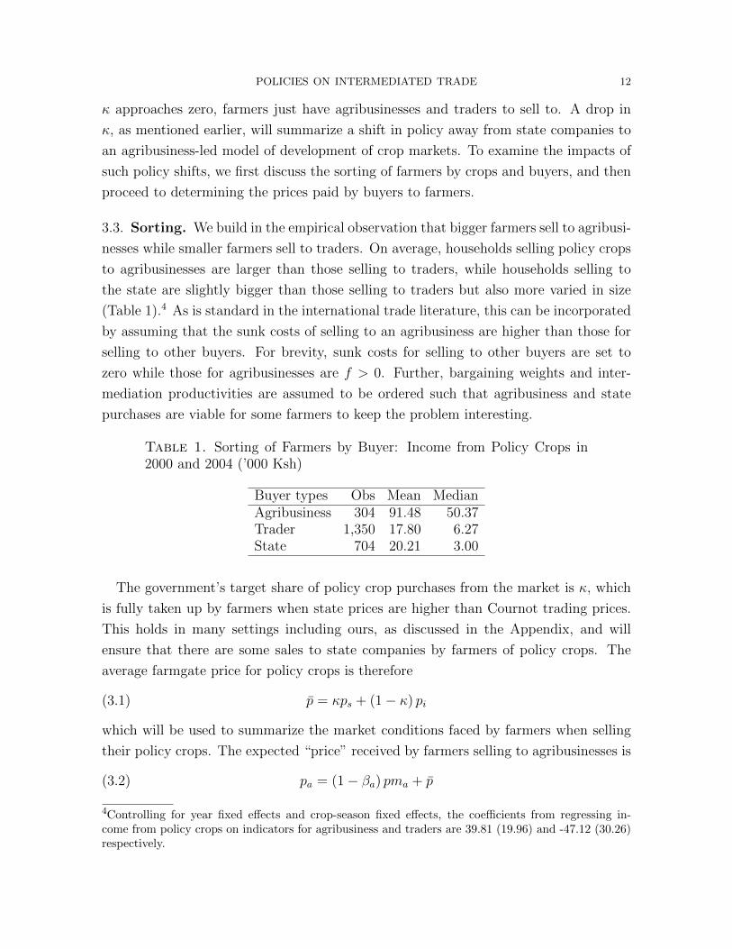
3.3. Sorting. We build in the empirical observation that bigger farmers sell to agribusi-
nesses while smaller farmers sell to traders. On average, households selling policy crops
to agribusinesses are larger than those selling to traders, while households selling to
the state are slightly bigger than those selling to traders but also more varied in size
(Table 1).4 As is standard in the international trade literature, this can be incorporated
by assuming that the sunk costs of selling to an agribusiness are higher than those for
selling to other buyers. For brevity, sunk costs for selling to other buyers are set to
zero while those for agribusinesses are f > 0. Further, bargaining weights and inter-
mediation productivities are assumed to be ordered such that agribusiness and state
purchases are viable for some farmers to keep the problem interesting.
Table 1. Sorting of Farmers by Buyer: Income from Policy Crops in2000 and 2004 (’000 Ksh)
Buyer types Obs Mean MedianAgribusiness 304 91.48 50.37Trader 1,350 17.80 6.27State 704 20.21 3.00
The government’s target share of policy crop purchases from the market is κ, which
is fully taken up by farmers when state prices are higher than Cournot trading prices.
This holds in many settings including ours, as discussed in the Appendix, and will
ensure that there are some sales to state companies by farmers of policy crops. The
average farmgate price for policy crops is therefore
(3.1) p̄ = κps + (1− κ) pi
which will be used to summarize the market conditions faced by farmers when selling
their policy crops. The expected “price” received by farmers selling to agribusinesses is
(3.2) pa = (1− βa) pma + p̄
4Controlling for year fixed effects and crop-season fixed effects, the coefficients from regressing in-come from policy crops on indicators for agribusiness and traders are 39.81 (19.96) and -47.12 (30.26)respectively.
POLICIES ON INTERMEDIATED TRADE 13
which consists of the surplus share and the going rate for trading services.5
Having defined the prices, farmers sort as follows into their cropping and intermedi-
ation choices. Farmers with productivity lower than
(3.3) ϕi ≡ 1/p̄
earn less in policy crops than in other crops, so they devote their land to other crops.
Farmers with productivity higher than ϕi prefer to grow policy crops. They choose
agribusinesses if their productivity is higher than
(3.4) ϕa ≡ f/ (pa − p̄)
so that they can meet the scale needed to justify the sunk investments. To sum up, the
lowest productivity farmers grow other crops, the medium productivity farmers choose
to grow policy crops but do not take up agribusiness services and the most productive
farmers grow policy crops and invest in agribusiness services.
3.4. Cournot Pricing. Having determined the cropping patterns and the sorting of
farmers by intermediaries, the price of trading services can be determined by solving
for a symmetric equilibrium. The supply of policy crops to the private market is
Q = (1− κ)
ˆ ∞ϕi
ϕdG (ϕ) = (1− κ)k
k − 1ϕkminp̄
k−1.
Therefore the perceived elasticity of demand for trading services is
∂ ln qi/∂ ln pi = (k − 1) (1− κ) (pi/p̄) (Q/qi) .
Cournot oligopsonists choose their optimal farmgate price such that the markdown on
intermediated world prices is equal to the inverse of their perceived demand elasticity:
(pm− pi) /pi = ∂ ln qi/∂ ln pi.
Substituting for the demand elasticity under a symmetric equilibrium, the optimal
price paid by oligopsonistic firms is
(3.5) pi =N (k − 1) pm− κps/ (1− κ)
N (k − 1) + 1.
In the benchmark case of perfect competition and no state companies, farmers receive
the world price, net of intermediation costs. Under infinite entry (N → ∞) or a
perfectly equal land distribution (k → ∞), prices do not change the extent to which
farmers alter their supply to intermediaries, so the full world price is transmitted to
5The qualitative results are similar when agribusinesses are assumed to pay for their trading servicesthrough Nash bargaining as well, but the expressions become much more tedious.
POLICIES ON INTERMEDIATED TRADE 14
farmers. When intermediaries are oligopsonistic (finite N and k), farmers receive a
smaller share of the price net of trade costs. Finally, holding entry fixed, prices paid
are lower when market size is smaller (due to higher government involvement κ).
3.5. Entry. Free entry of intermediaries ensures average profits are driven down to
entry costs. Ignoring the integer constraint, free entry in trading services gives
(3.6) (1− κ)k
k − 1ϕkmin (pm− pi)ϕ−k+1
i /N = F
where
pm− pi =pm+ κps/ (1− κ)
N (k − 1) + 1
is the markdown in farmgate prices arising from oligopsonistic pricing. Similarly, free
entry into agribusiness operations ensures average profit from agribusiness activities is
driven down to entry costs,
(3.7)k
k − 1ϕkmin (1− κ) (pma − (pa − p̄))ϕ−k+1
a /M = Fa.
To ensure that the number of firms exceeds one, we assume entry costs are not too high
to completely preclude entry into the crop market.6
Having discussed the entry conditions, the equilibrium of the economy can be speci-
fied in terms of the optimal cutoffs, optimal prices and optimal entry. These are given
jointly by the cutoff equations 3.3 and 3.4, the pricing equations 3.1, 3.2 and 3.5 and
the free entry equations 3.6 and 3.7.
3.6. Incomes. We are interested in examining income changes experienced by farmers
as a result of a policy shift away from state companies towards private companies in
development of crop markets. As mentioned earlier, this can be summarized by a drop
in the probability of being able to sell to state companies κ, so we discuss comparative
statics of incomes with respect to κ. Much of the analysis will summarize income
changes in terms of changes in market conditions, ∂ ln p̄/∂ lnκ, which will be a useful
statistic to understand the welfare implications of the policy change.
Incomes of farmers selling policy crops to agribusinesses is
Ia =
ˆ ∞ϕa
(paϕ− f) dG.
6Conditions to ensure this in terms of primitives are in the Appendix.
POLICIES ON INTERMEDIATED TRADE 15
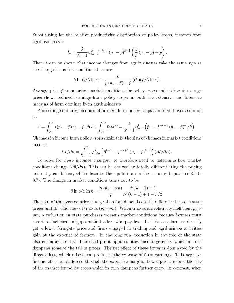
Substituting for the relative productivity distribution of policy crops, incomes from
agribusinesses is
Ia =k
k − 1ϕkminf
−k+1 (pa − p̄)k−1(
1
k(pa − p̄) + p̄
).
Then it can be shown that income changes from agribusinesses take the same sign as
the change in market conditions because
∂ ln Ia/∂ lnκ =p̄
1k
(pa − p̄) + p̄(∂ ln p̄/∂ lnκ) .
Average price p̄ summarizes market conditions for policy crops and a drop in average
price shows reduced earnings from policy crops on both the extensive and intensive
margins of farm earnings from agribusinesses.
Proceeding similarly, incomes of farmers from policy crops across all buyers sum up
to
I =
ˆ ∞ϕa
((pa − p̄)ϕ− f) dG+
ˆ ∞ϕi
p̄ϕdG =k
k − 1ϕkmin
(p̄k + f−k+1 (pa − p̄)k /k
).
Changes in income from policy crops again take the sign of changes in market conditions
because
∂I/∂κ =k2
k − 1ϕkmin
(p̄k−1 + f−k+1 (pa − p̄)k−1
)(∂p̄/∂κ) .
To solve for these incomes changes, we therefore need to determine how market
conditions change (∂p̄/∂κ). This can be derived by totally differentiating the pricing
and entry conditions, which describe the equilibrium in the economy (equations 3.1 to
3.7). The change in market conditions turns out to be
∂ ln p̄/∂ lnκ =κ (ps − pm)
p̄
N (k − 1) + 1
N (k − 1) + 1− k/2.
The sign of the average price change therefore depends on the difference between state
prices and the efficiency of traders (ps−pm). When traders are relatively inefficient ps >
pm, a reduction in state purchases worsens market conditions because farmers must
resort to inefficient oligopsonistic traders who pay less. In this case, farmers directly
get a lower farmgate price and firms engaged in trading and agribusiness activities
gain at the expense of farmers. In the long run, reduction in the role of the state
also encourages entry. Increased profit opportunities encourage entry which in turn
dampens some of the fall in prices. The net effect of these forces is dominated by the
direct effect, which raises firm profits at the expense of farm earnings. This negative
income effect is reinforced through the extensive margin. Lower prices reduce the size
of the market for policy crops which in turn dampens further entry. In contrast, when
POLICIES ON INTERMEDIATED TRADE 16
traders are sufficiently efficient pm > ps, the direct effect of a reduction in the role of
the state is smaller than the indirect effect from entry of firms which raises the price
received by farmers.
Summing up, incomes from policy crops, including for farmers who engage with
agribusinesses, fall after the policy shift when traders are relatively inefficient and vice-
versa. This will be the first part of the empirical application, which examines the
incomes earned by farmers in policy crops, relative to other crops, and we summarize
it in Proposition 1 below.
Proposition 1. When traders are relatively inefficient, incomes of farmers from pol-
icy crops fall with a policy shift towards private sector-led intermediation (lower κ).
Agribusiness profits rise till they are eroded away through greater entry after the policy
shift. The opposite results hold for relatively efficient traders.
Our empirical setting corresponds with relatively inefficient traders and we will show
in section 4 that incomes from policy crops are lower after the policy change in the em-
pirical application. More generally, however, the theoretical framework can be extended
to also allow for rent sharing in agribusiness activities to be affected by competition
among agribusinesses. Then prices paid to farmers for making agribusiness investments
rise with a reduction in state purchases. This is because the increase in market size
for agribusinesses encourages entry and therefore the surplus share that they pay to
farmers. There are then two opposing forces affecting farm incomes after the rollback
in state participation – average prices p̄ change as described earlier but agribusiness
prices pa − p̄ rise due to increased competition among firms. Moreover, if the policy
shift is additionally considered to have reduced entry costs for agribusiness activities Fa,
then the positive competitive forces that raise the rents paid to farmers are reinforced.
Which force dominates, changes in trading prices or rent sharing from agribusinesses,
depends on the shares and elasticities of each activity in farm incomes, and is there-
fore an empirical question.7 This will be implemented through a difference-in-difference
specification, which compares farm earnings and firm profits from policy crops and
other crops, before and after the policy change.
3.7. Comparative Advantage and Incomes. We are ultimately interested in ex-
amining how changes in agricultural intermediation policies impact the overall welfare
of farmers. A natural metric for farmer welfare is the total income across all crops.
7For example, Macchiavello and Morjaria (2015) find competition among coffee mills in Rwanda un-dermined relational contracts between mills and farmers, leading to lower farmer welfare.
POLICIES ON INTERMEDIATED TRADE 17
Aggregating up farm incomes across crops, the total income from farming is
Y =
ˆ ∞ϕa
((pa − p̄)ϕ− f) dG+
ˆ ∞ϕi
p̄ϕdG+
ˆ ϕi
ϕmin
dG = 1+1
k − 1ϕkmin
[p̄k + f−k+1 (pa − p̄)k
].
The change in farm income again takes on the sign of the average price change because
Y ′/Y ≡ ∂ lnY/∂ lnκ =
(k
k − 1ϕkminp̄
k/Y
)(∂ ln p̄/∂ lnκ)
where the first term in parenthesis on the RHS corresponds to the share of farm incomes
arising from trading of policy crops. If the total farm income is compared over time,
then incomes are expected to fall or rise after the policy shift, depending on how
average prices respond to the policy shift. But simply using time variation in incomes
makes it difficult to ascribe the income change to the policy shift, rather than to other
time varying changes in the economy. We therefore minimize concerns regarding time-
varying factors other than the policy shift affecting incomes by using the theoretical
framework to guide empirical examination. In particular, we compare farm incomes by
comparative advantage in policy crops. Farmers with a higher comparative advantage
would be more reliant and more affected by policies pertaining to those crops.
Following recent work using agronomical databases to determine crop choices, farm
income changes can be compared across villages with higher or lower comparative ad-
vantage in the policy crops. The theoretical framework implies such a comparison. For
example, comparing two villages that differ in ϕmin, it can be shown that income shares
from policy crops, entry and average prices for policy crops are higher in comparative
advantage villages. Looking further at how incomes in the two villages evolve after the
policy shift, it can be shown that income changes depend on the extent to which the
shares of policy crops in incomes and the responsiveness of average prices to state pur-
chases differ by comparative advantage. Comparative advantage villages have higher
shares of their incomes from policy crops. Furthermore, the responsiveness of their
average price change to state purchases is also larger, (except under a very unequal
productivity distribution). The price effect, in either case, does not overturn the first
order effect of large income shares from policy crops which make these villages more
exposed to the policy change. Specifically,
∂ lnY ′/∂ lnϕmin =k
2
N − 1
(N (k − 1) + 1− k/2)2
(k − N − 2
N − 1
)> 0
for all k ≥ 1. Therefore, when the national government reduces its purchases (κ falls),
comparative advantage villages see bigger total income changes, even after accounting
POLICIES ON INTERMEDIATED TRADE 18
for different pricing and entry strategies of firms across villages. This prediction, sum-
marized in Proposition 2 below, can be taken to the data and implemented through a
standard difference-in-difference strategy, which compares total incomes in comparative
advantage villages and other villages, before and after the policy shift.
Proposition 2. Farmers in villages with a comparative advantage in policy crops
(higher ϕmin) face bigger impacts on their total incomes.
Having provided a theoretical framework to understand income changes, the next
section proceeds to empirically examining Propositions 1 and 2.
4. Empirics
This section starts with examining Proposition 1, which relates incomes earned at the
crop level by households before and after the policy shift. The impacts on crop incomes
from all buyers and from agribusinesses are discussed in turn. Then it proceeds to
examining the profits of agribusinesses, by their specialisation in policy crops, before
and after the policy shift. The final sub-section examines Proposition 2, which compares
income and welfare impacts at the level of the household across comparative advantage
villages and other villages.
4.1. Crop Incomes and Policy. To operationalize Proposition 1, we implement a
difference-in-difference (DiD) analysis comparing incomes received from policy crops
with other crops, before and after the policy shift. Let c index crops (example, dry
maize) and g index the group - Policy crops or Other crops - to which each crop
belongs. Let Postt be an indicator for the period after the policy shift which consists
of the main and short cropping seasons for the year 2006-2007 (from July 2006 to June
2007), while the period before consists of the main and short seasons in 1999-2000 and
2003-2004. Then Incomecghst (in Ksh) is the income received for crop c in group g by
household h in season s of year t, which is specified as follows:
Incomecghst =β PosttPolicyg + αcs + αh + αt + εcghst(4.1)
Policyg = 1 for the 18 crops that experienced a policy shift from the Strategy for
Revitalizing Agriculture in 2004 and 0 otherwise. β is the coefficient of interest which
is negative when incomes from policy crops fall relative to other crops after the policy
shift and ε is an error term. Crop-season fixed effects are included to account for
time-invariant differences in incomes across crops in each season, and standard errors
POLICIES ON INTERMEDIATED TRADE 19
are clustered by crops.8 Year fixed effects account for general macroeconomic changes
in the country. Household fixed effects ensure that we are examining income changes
within households.
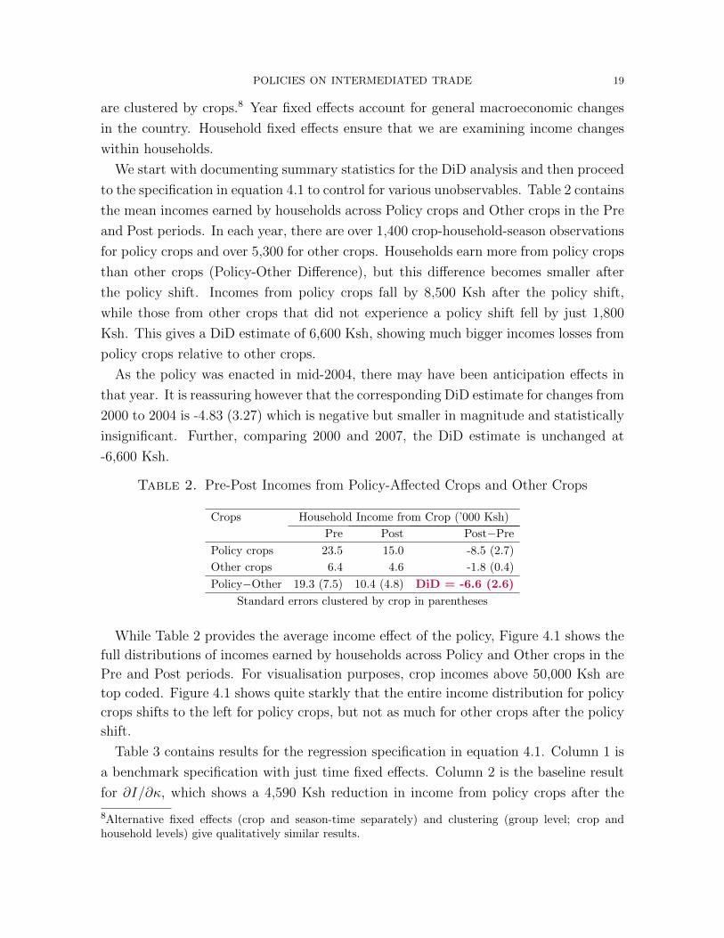
We start with documenting summary statistics for the DiD analysis and then proceed
to the specification in equation 4.1 to control for various unobservables. Table 2 contains
the mean incomes earned by households across Policy crops and Other crops in the Pre
and Post periods. In each year, there are over 1,400 crop-household-season observations
for policy crops and over 5,300 for other crops. Households earn more from policy crops
than other crops (Policy-Other Difference), but this difference becomes smaller after
the policy shift. Incomes from policy crops fall by 8,500 Ksh after the policy shift,
while those from other crops that did not experience a policy shift fell by just 1,800
Ksh. This gives a DiD estimate of 6,600 Ksh, showing much bigger incomes losses from
policy crops relative to other crops.
As the policy was enacted in mid-2004, there may have been anticipation effects in
that year. It is reassuring however that the corresponding DiD estimate for changes from
2000 to 2004 is -4.83 (3.27) which is negative but smaller in magnitude and statistically
insignificant. Further, comparing 2000 and 2007, the DiD estimate is unchanged at
-6,600 Ksh.
Table 2. Pre-Post Incomes from Policy-Affected Crops and Other Crops
Crops Household Income from Crop (’000 Ksh)
Pre Post Post−Pre
Policy crops 23.5 15.0 -8.5 (2.7)
Other crops 6.4 4.6 -1.8 (0.4)
Policy−Other 19.3 (7.5) 10.4 (4.8) DiD = -6.6 (2.6)
Standard errors clustered by crop in parentheses
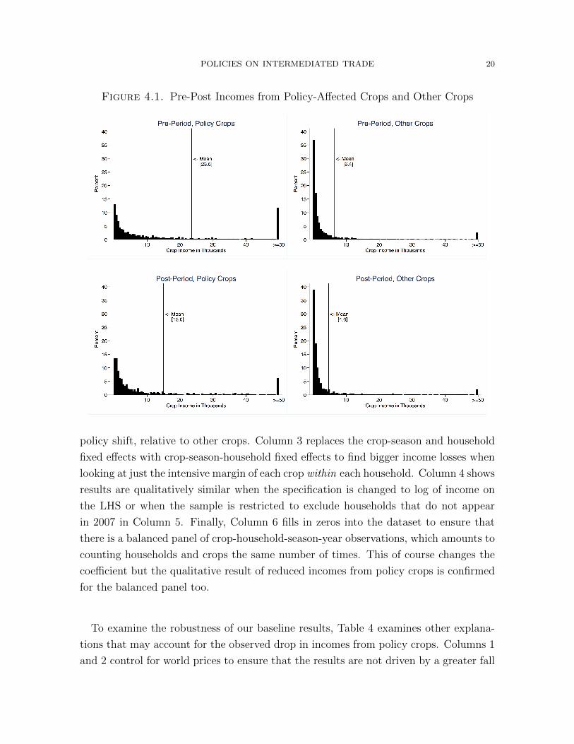
While Table 2 provides the average income effect of the policy, Figure 4.1 shows the
full distributions of incomes earned by households across Policy and Other crops in the
Pre and Post periods. For visualisation purposes, crop incomes above 50,000 Ksh are
top coded. Figure 4.1 shows quite starkly that the entire income distribution for policy
crops shifts to the left for policy crops, but not as much for other crops after the policy
shift.
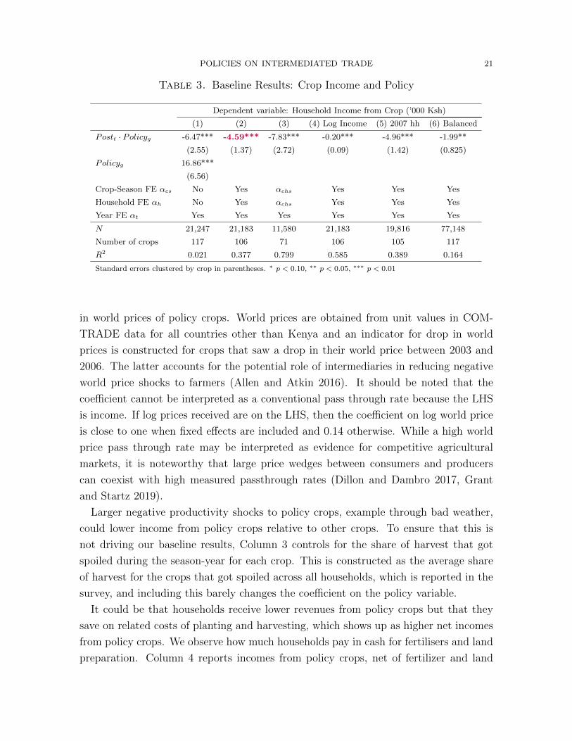
Table 3 contains results for the regression specification in equation 4.1. Column 1 is
a benchmark specification with just time fixed effects. Column 2 is the baseline result
for ∂I/∂κ, which shows a 4,590 Ksh reduction in income from policy crops after the
8Alternative fixed effects (crop and season-time separately) and clustering (group level; crop andhousehold levels) give qualitatively similar results.
POLICIES ON INTERMEDIATED TRADE 20
Figure 4.1. Pre-Post Incomes from Policy-Affected Crops and Other Crops
policy shift, relative to other crops. Column 3 replaces the crop-season and household
fixed effects with crop-season-household fixed effects to find bigger income losses when
looking at just the intensive margin of each crop within each household. Column 4 shows
results are qualitatively similar when the specification is changed to log of income on
the LHS or when the sample is restricted to exclude households that do not appear
in 2007 in Column 5. Finally, Column 6 fills in zeros into the dataset to ensure that
there is a balanced panel of crop-household-season-year observations, which amounts to
counting households and crops the same number of times. This of course changes the
coefficient but the qualitative result of reduced incomes from policy crops is confirmed
for the balanced panel too.
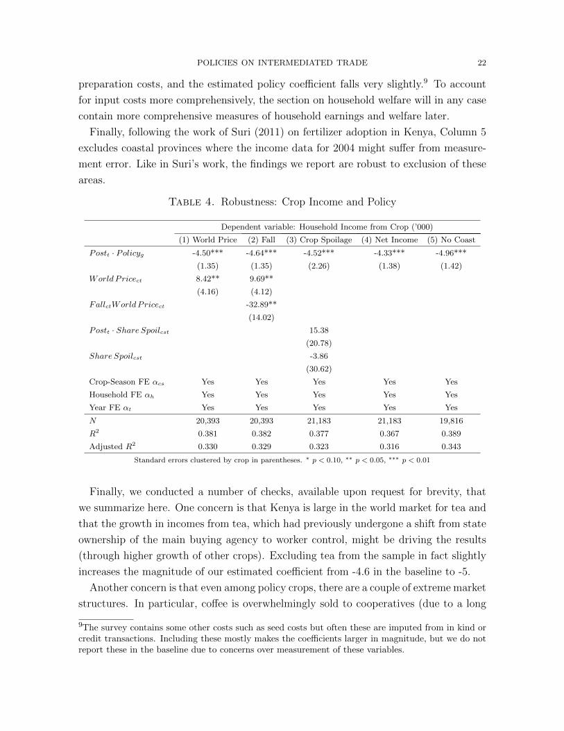
To examine the robustness of our baseline results, Table 4 examines other explana-
tions that may account for the observed drop in incomes from policy crops. Columns 1
and 2 control for world prices to ensure that the results are not driven by a greater fall
POLICIES ON INTERMEDIATED TRADE 21
Table 3. Baseline Results: Crop Income and Policy
Dependent variable: Household Income from Crop (’000 Ksh)
(1) (2) (3) (4) Log Income (5) 2007 hh (6) Balanced
Postt · Policyg -6.47*** -4.59*** -7.83*** -0.20*** -4.96*** -1.99**
(2.55) (1.37) (2.72) (0.09) (1.42) (0.825)
Policyg 16.86***
(6.56)
Crop-Season FE αcs No Yes αchs Yes Yes Yes
Household FE αh No Yes αchs Yes Yes Yes
Year FE αt Yes Yes Yes Yes Yes Yes
N 21,247 21,183 11,580 21,183 19,816 77,148
Number of crops 117 106 71 106 105 117
R2 0.021 0.377 0.799 0.585 0.389 0.164
Standard errors clustered by crop in parentheses. ∗ p < 0.10, ∗∗ p < 0.05, ∗∗∗ p < 0.01
in world prices of policy crops. World prices are obtained from unit values in COM-
TRADE data for all countries other than Kenya and an indicator for drop in world
prices is constructed for crops that saw a drop in their world price between 2003 and
2006. The latter accounts for the potential role of intermediaries in reducing negative
world price shocks to farmers (Allen and Atkin 2016). It should be noted that the
coefficient cannot be interpreted as a conventional pass through rate because the LHS
is income. If log prices received are on the LHS, then the coefficient on log world price
is close to one when fixed effects are included and 0.14 otherwise. While a high world
price pass through rate may be interpreted as evidence for competitive agricultural
markets, it is noteworthy that large price wedges between consumers and producers
can coexist with high measured passthrough rates (Dillon and Dambro 2017, Grant
and Startz 2019).
Larger negative productivity shocks to policy crops, example through bad weather,
could lower income from policy crops relative to other crops. To ensure that this is
not driving our baseline results, Column 3 controls for the share of harvest that got
spoiled during the season-year for each crop. This is constructed as the average share
of harvest for the crops that got spoiled across all households, which is reported in the
survey, and including this barely changes the coefficient on the policy variable.
It could be that households receive lower revenues from policy crops but that they
save on related costs of planting and harvesting, which shows up as higher net incomes
from policy crops. We observe how much households pay in cash for fertilisers and land
preparation. Column 4 reports incomes from policy crops, net of fertilizer and land
POLICIES ON INTERMEDIATED TRADE 22
preparation costs, and the estimated policy coefficient falls very slightly.9 To account
for input costs more comprehensively, the section on household welfare will in any case
contain more comprehensive measures of household earnings and welfare later.
Finally, following the work of Suri (2011) on fertilizer adoption in Kenya, Column 5
excludes coastal provinces where the income data for 2004 might suffer from measure-
ment error. Like in Suri’s work, the findings we report are robust to exclusion of these
areas.
Table 4. Robustness: Crop Income and Policy
Dependent variable: Household Income from Crop (’000)
(1) World Price (2) Fall (3) Crop Spoilage (4) Net Income (5) No Coast
Postt · Policyg -4.50*** -4.64*** -4.52*** -4.33*** -4.96***
(1.35) (1.35) (2.26) (1.38) (1.42)
WorldPricect 8.42** 9.69**
(4.16) (4.12)
FallctWorldPricect -32.89**
(14.02)
Postt · Share Spoilcst 15.38
(20.78)
Share Spoilcst -3.86
(30.62)
Crop-Season FE αcs Yes Yes Yes Yes Yes
Household FE αh Yes Yes Yes Yes Yes
Year FE αt Yes Yes Yes Yes Yes
N 20,393 20,393 21,183 21,183 19,816
R2 0.381 0.382 0.377 0.367 0.389
Adjusted R2 0.330 0.329 0.323 0.316 0.343
Standard errors clustered by crop in parentheses. ∗ p < 0.10, ∗∗ p < 0.05, ∗∗∗ p < 0.01
Finally, we conducted a number of checks, available upon request for brevity, that
we summarize here. One concern is that Kenya is large in the world market for tea and
that the growth in incomes from tea, which had previously undergone a shift from state
ownership of the main buying agency to worker control, might be driving the results
(through higher growth of other crops). Excluding tea from the sample in fact slightly
increases the magnitude of our estimated coefficient from -4.6 in the baseline to -5.
Another concern is that even among policy crops, there are a couple of extreme market
structures. In particular, coffee is overwhelmingly sold to cooperatives (due to a long
9The survey contains some other costs such as seed costs but often these are imputed from in kind orcredit transactions. Including these mostly makes the coefficients larger in magnitude, but we do notreport these in the baseline due to concerns over measurement of these variables.
POLICIES ON INTERMEDIATED TRADE 23
tradition of non-governmental agencies in this sector) while sugar is overwhelmingly sold
to agribusinesses (due to the need for immediate processing of the harvest). Excluding
coffee barely moves the estimated policy coefficient as just about 5 per cent of the sample
constitutes coffee. Alternatively, we include an interaction term between an indicator
for coffee and the policy variable - PosttPolicygCoffeec. The estimated coefficient on
the interaction is -0.32 (with a standard error of 2.67). This suggests the policy shift
showed negligible income reductions when the buyers, who are largely cooperatives, do
not exert monopsony power. Excluding sugar changes the policy coefficient to -3.88
(1.16), which is qualitatively similar to the baseline but somewhat smaller.
There is another concern that our baseline results might reflect what happened in
maize markets, which is the main food crop grown by households and also the chief
source of income for the previous President Moi’s home base. Excluding maize still
gives negative income impacts of the policy, and the estimated coefficient increases in
magnitude to -5.8. Therefore, the robustness exercises reveal that crop-specific pecu-
liarities do not seem to be the driving force behind our baseline results.
4.2. Crop Incomes, Policy and Agribusiness. To examine differences across agribusi-
ness and other buyers, let Agribusinesschst = 1 when the crop is sold mainly to an
agribusiness, which refers to large companies, exporters, millers and processors in the
survey.10 Theoretically, income reduction from the policy shift is lower for farmers sell-
ing through agribusinesses, because average trading prices fall more than rents from
agribusinesses. This raises the share of agribusinesses in income from policy crops af-
ter the policy shift (Ia/I rise with lower κ). However, incomes from policy crops fall
for farmers selling to agribusinesses and other buyers. Allowing for heterogeneity in
the policy coefficient across purchases made by agribusinesses and other buyers, the
specification in equation 4.1 can be extended as follows:
Incomecghst =βaPosttPolicygAgribusinesschst + γ1PolicygAgribusinesschst
+ β PosttPolicygOtherBuyerschst + γ2PolicygOtherBuyerschst
+ γ3PosttAgribusinesschst + γ4Agribusinesschst
+ γ5PosttOtherBuyerschst + γ6OtherBuyerschst
+ αcs + αh + αt + εcghst
10As our focus is on a policy shift from state to private-sector purchases, co-operatives, boards andworker controlled agencies like the National Cereals and Produce Board or the Kenya Tea DevelopmentAgency Holdings Limited are excluded from the agribusiness category.
POLICIES ON INTERMEDIATED TRADE 24
where βa would be the estimated income impact of the policy for households who sell
the crop mainly to agribusinesses and β would be the estimated income impact of the
policy for households selling the crop to buyers other than agribusinesses.
The share of agribusinesses rises during the period and agribusinesses become the
majority buyer of policy crops. The share of agribusinesses in farm purchases rises from
40 per cent to 51.5 per cent in policy crops. Other crops also see a rise in agribusiness
shares from 2 per cent to 9.8 per cent, but the levels remain much lower. Regressing
an indicator for agribusiness purchases on PosttPolicyg and the set of fixed effects
(crop-season, household and time), the estimated coefficient on the policy variable is
5 per cent, which rises to 9 per cent when the contribution of each crop to total farm
income of the household is used as weights for the regression. Following the discussion
on robustness, when PosttPolicygCoffeec is included in the regression, the estimated
likelihood of agribusiness purchases rises to 8.2 per cent (unweighted) and 12.3 per cent
(weighted by crop share).
Households selling to agribusinesses experience a drop in income from policy crops
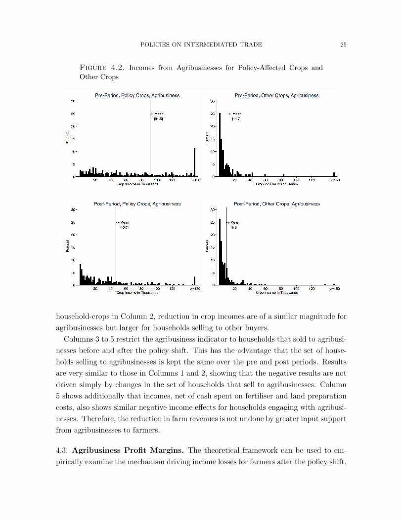
after the policy shift, as expected. This can be seen in Figure 4.2, which plots the
distributions of incomes for households selling to agribusinesses. Households selling to
agribusinesses have much higher incomes from policy crops, but they also experience
much bigger reductions in their incomes from policy crops. The distribution of income
from policy crops shifts to the left while incomes from other crops shows a much more
muted shift to the left, after the policy shift. The finding of large income losses for
households selling policy crops to agribusinesses is consistent with the large 40 per cent
reduction in cotton yields that farmers faced when outgrower schemes failed in Zambia
(Brambilla and Porto 2011).
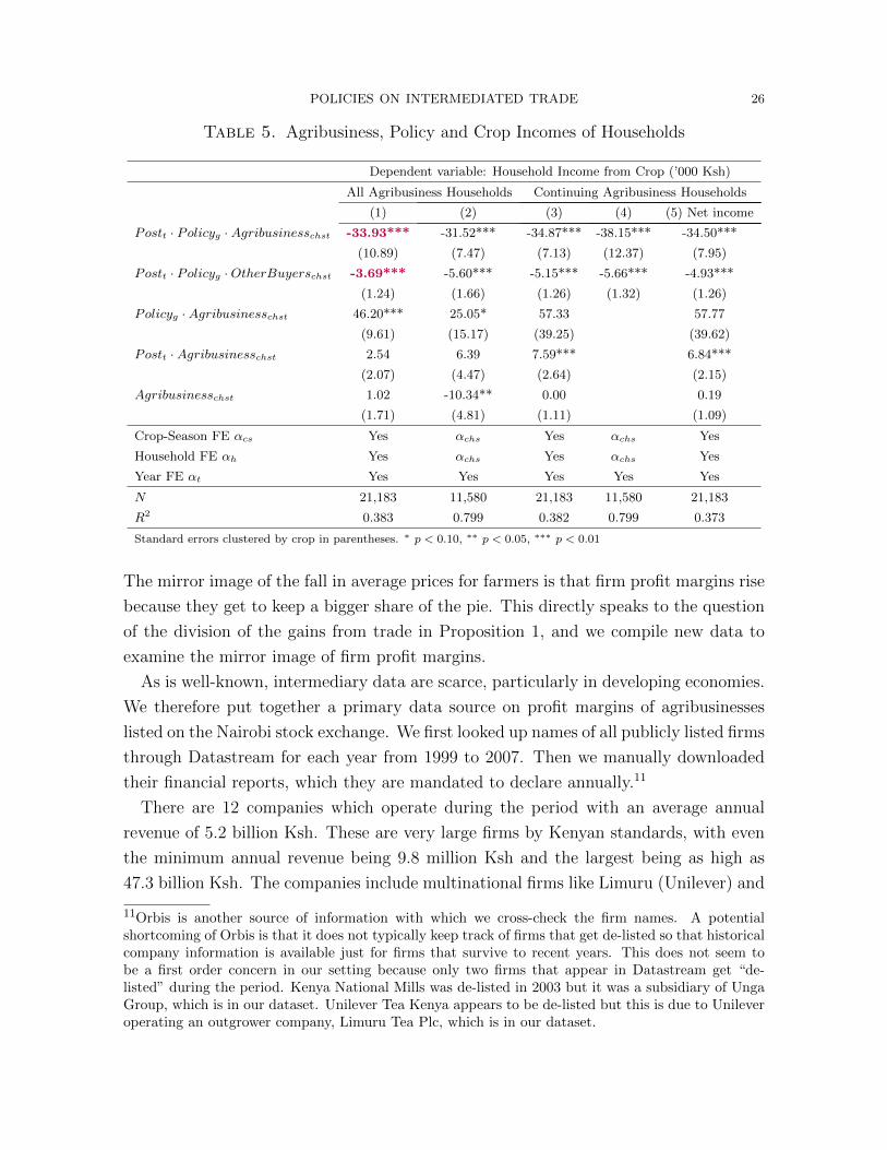
Table 5 shows the income impact of the policy after separating out purchases made
by agribusiness and other buyers. For crops sold to agribusinesses, Column 1 shows
households experience an average 34,000 Ksh reduction in income from policy crops
after the policy shift, relative to other crops. The magnitude is much larger because
sales of policy crops to agribusinesses also tend to be much larger, as expected from the
sorting patterns of households to agribusinesses. This can be seen from the γ1 coefficient
on PolicygAgribusinesschst which is 46,000 Ksh. Households selling to other buyers are
also impacted negatively. The magnitude is much smaller at 3,690 Ksh, reflecting their
much lower levels of crop incomes. Evaluated at the mean incomes of households selling
to agribusinesses and to other buyers, the estimated income elasticity at the mean of
the PosttPolicyg variable is -7 per cent for households selling to agribusinesses and
-11 per cent for those selling to other buyers. Looking just at the intensive margin of
POLICIES ON INTERMEDIATED TRADE 25
Figure 4.2. Incomes from Agribusinesses for Policy-Affected Crops and
Other Crops
household-crops in Column 2, reduction in crop incomes are of a similar magnitude for
agribusinesses but larger for households selling to other buyers.
Columns 3 to 5 restrict the agribusiness indicator to households that sold to agribusi-
nesses before and after the policy shift. This has the advantage that the set of house-
holds selling to agribusinesses is kept the same over the pre and post periods. Results
are very similar to those in Columns 1 and 2, showing that the negative results are not
driven simply by changes in the set of households that sell to agribusinesses. Column
5 shows additionally that incomes, net of cash spent on fertiliser and land preparation
costs, also shows similar negative income effects for households engaging with agribusi-
nesses. Therefore, the reduction in farm revenues is not undone by greater input support
from agribusinesses to farmers.
4.3. Agribusiness Profit Margins. The theoretical framework can be used to em-
pirically examine the mechanism driving income losses for farmers after the policy shift.
POLICIES ON INTERMEDIATED TRADE 26
Table 5. Agribusiness, Policy and Crop Incomes of Households
Dependent variable: Household Income from Crop (’000 Ksh)
All Agribusiness Households Continuing Agribusiness Households
(1) (2) (3) (4) (5) Net income
Postt · Policyg ·Agribusinesschst -33.93*** -31.52*** -34.87*** -38.15*** -34.50***
(10.89) (7.47) (7.13) (12.37) (7.95)
Postt · Policyg ·OtherBuyerschst -3.69*** -5.60*** -5.15*** -5.66*** -4.93***
(1.24) (1.66) (1.26) (1.32) (1.26)
Policyg ·Agribusinesschst 46.20*** 25.05* 57.33 57.77
(9.61) (15.17) (39.25) (39.62)
Postt ·Agribusinesschst 2.54 6.39 7.59*** 6.84***
(2.07) (4.47) (2.64) (2.15)
Agribusinesschst 1.02 -10.34** 0.00 0.19
(1.71) (4.81) (1.11) (1.09)
Crop-Season FE αcs Yes αchs Yes αchs Yes
Household FE αh Yes αchs Yes αchs Yes
Year FE αt Yes Yes Yes Yes Yes
N 21,183 11,580 21,183 11,580 21,183
R2 0.383 0.799 0.382 0.799 0.373
Standard errors clustered by crop in parentheses. ∗ p < 0.10, ∗∗ p < 0.05, ∗∗∗ p < 0.01
The mirror image of the fall in average prices for farmers is that firm profit margins rise
because they get to keep a bigger share of the pie. This directly speaks to the question
of the division of the gains from trade in Proposition 1, and we compile new data to
examine the mirror image of firm profit margins.
As is well-known, intermediary data are scarce, particularly in developing economies.
We therefore put together a primary data source on profit margins of agribusinesses
listed on the Nairobi stock exchange. We first looked up names of all publicly listed firms
through Datastream for each year from 1999 to 2007. Then we manually downloaded
their financial reports, which they are mandated to declare annually.11
There are 12 companies which operate during the period with an average annual
revenue of 5.2 billion Ksh. These are very large firms by Kenyan standards, with even
the minimum annual revenue being 9.8 million Ksh and the largest being as high as
47.3 billion Ksh. The companies include multinational firms like Limuru (Unilever) and
11Orbis is another source of information with which we cross-check the firm names. A potentialshortcoming of Orbis is that it does not typically keep track of firms that get de-listed so that historicalcompany information is available just for firms that survive to recent years. This does not seem tobe a first order concern in our setting because only two firms that appear in Datastream get “de-listed” during the period. Kenya National Mills was de-listed in 2003 but it was a subsidiary of UngaGroup, which is in our dataset. Unilever Tea Kenya appears to be de-listed but this is due to Unileveroperating an outgrower company, Limuru Tea Plc, which is in our dataset.
POLICIES ON INTERMEDIATED TRADE 27
Kakuzi (UK-based Camellia Plc) and domestic conglomerates like the Unga group and
Uchumi supermarkets, which are well-recognized brands in Kenya.
Although firms report their accounts in different ways, two key variables are available
consistently over time and across firms. The first key variable is the profit margin of
the firm (profit before tax reported by the company divided by its revenue), which is
our dependent variable. The median profit margin of companies is 5.5 per cent and
the mean is 3.9 per cent. There is a wide range of margins, so we conduct robustness
exercises later by trimming the outlier values.
The second key variable is the cropping segment in which the company operates,
which is available from company sales reports and sales descriptions. Segment refers
to Beer and Beverages, Coffee, Horticulture, Sisal, Cotton spinning and services, Sugar
made from cane, Tea, Maize milling, Wheat production, Poultry feeds and Animal
health, or All of these. If the segment includes policy crops, then 1seg,g=1 = 1 and 0
otherwise. The policy exposure of company j can be defined as the share of sales in
policy-affected segments in the pre period (1999-2004),
Policyj =∑seg
1seg,g=1Salesseg,g,j/Total Salesj.
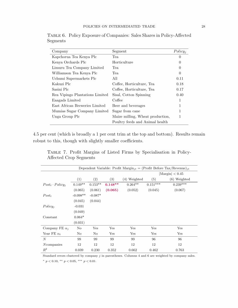
The median policy exposure is 18 per cent and the mean is 33 per cent. Table 6 contains
the list of companies, their segments and their policy exposure values. Most companies
specialize in one segment so they get values of 0 or 1. For companies that operate in
more than one segment, the policy variable reflects the sales share of policy-affected
crops. Uchumi Supermarkets operates in all segments, so we assign it the average share
of policy crops in the economy.
Having defined the key variables, the impact of the policy shift on agribusiness profits
can be estimated as follows: ProfitMarginjt = β · Postt · Policyj + αt + αj + εjt
where αj refers to firm fixed effects. The coefficient of interest is β, which captures
the extent to which profit margins rise more for firms that are more exposed to the
policy based on their crop specialisation. Table 7 contains the results. In our baseline
specification of Column 3, profit margins of firms that were specialized in policy crops
rises by 15 per cent more than firms that were specialised in other crops. If Uchumi
supermarkets is excluded from the sample, the estimated coefficient falls slightly to 13
per cent. Column 4 reports results using initial firm revenues as regression weights.
This raises the estimate to 26.4 per cent as higher revenue firms tend to have higher
profits. Finally, Columns 5 and 6 restrict profit margins to absolute values lower than
POLICIES ON INTERMEDIATED TRADE 28
Table 6. Policy Exposure of Companies: Sales Shares in Policy-AffectedSegments
Company Segment Policyj
Kapchorua Tea Kenya Plc Tea 0
Kenya Orchards Plc Horticulture 0
Limuru Tea Company Limited Tea 0
Williamson Tea Kenya Plc Tea 0
Uchumi Supermarkets Plc All 0.11
Kakuzi Plc Coffee, Horticulture, Tea 0.18
Sasini Plc Coffee, Horticulture, Tea 0.17
Rea Vipingo Plantations Limited Sisal, Cotton Spinning 0.40
Eaagads Limited Coffee 1
East African Breweries Limited Beer and beverages 1
Mumias Sugar Company Limited Sugar from cane 1
Unga Group Plc Maize milling, Wheat production, 1
Poultry feeds and Animal health
4.5 per cent (which is broadly a 1 per cent trim at the top and bottom). Results remain
robust to this, though with slightly smaller coefficients.
Table 7. Profit Margins of Listed Firms by Specialisation in Policy-Affected Crop Segments
Dependent Variable: Profit Marginjt = (Profit Before Tax/Revenue)jt
|Margin| < 0.45
(1) (2) (3) (4) Weighted (5) (6) Weighted
Postt · Policyj 0.149** 0.153** 0.148** 0.264** 0.151*** 0.239***
(0.065) (0.061) (0.065) (0.052) (0.045) (0.067)
Postt -0.098** -0.087*
(0.045) (0.044)
Policyj -0.031
(0.049)
Constant 0.064*
(0.031)
Company FE αj No Yes Yes Yes Yes Yes
Year FE αt No No Yes Yes Yes Yes
N 99 99 99 99 96 96
Ncompanies 12 12 12 12 12 12
R2 0.039 0.230 0.352 0.662 0.462 0.763
Standard errors clustered by company j in parentheses. Columns 4 and 6 are weighted by company sales.
∗ p < 0.10, ∗∗ p < 0.05, ∗∗∗ p < 0.01.
POLICIES ON INTERMEDIATED TRADE 29
At the mean policy exposure level of 0.33, the estimated rise in profits is 5 per
cent (unweighted) to 9 per cent (weighted) greater for agribusinesses specialising in the
policy crops. We conclude that the shift to an agribusiness model reallocated profits
away from farmers towards agribusiness firms. It is striking that despite an expansion
in market size for private-sector firms, incumbent agribusinesses saw a rise in profit
margins after the policy shift.
4.4. Household Welfare. Proposition 2 explains that households with a comparative
advantage in policy crops would have a greater income dependence on these crops
and experience a greater reduction in income. We therefore examine household level
outcomes by their comparative advantage in policy crops.
Comparative advantage in policy crops can be measured following a growing literature
that uses agroecological data from FAOSTAT to define the potential yields across crops
based on soil, weather and other climactic conditions of the area (example, Nunn and
Qian 2011). FAOSTAT provides data on potential yields for major crops of the world
since the 1960s. This covers 35 crops from our sample, which make up 88 per cent of
all farm incomes which can be mapped on to 90 per cent of households (who make up
92 per cent of farm incomes).
The finest level of geographical disaggregation at which we can map households in
our sample is the village. There are 107 distinct villages which can all be mapped on to
the FAO potential yield data. We use the mean potential yields for rain-fed, low input
use agriculture for the 1961-2000 baseline of FAOSTAT for all available crops in each
village. As discussed in the theoretical section, cropping choices depend on the price
and productivity of households (pϕ). For each village, we construct the difference in
potential yield values across policy and other crops as
Potential Y ieldv ≡∑
c∈Policy crops
pcϕcv −∑
c∈Other crops
pcϕcv
where pc is the world price of crop c and ϕcv is its mean potential yield in village v.
We categorise villages into those with above and below median Potential Y ieldv, and
CAv is an indicator for villages with above median Potential Y ieldv. Proposition 2
can therefore be operationalized as a DiD regression comparing household outcomes in
villages based on their comparative advantage in policy crops CAv.
For outcome Yhvt of household h in village v at time t, the DiD can be implemented
as a regression through the following specification:
Yhvt =β0PosttCAv + αh + αt + εhvt(4.2)
POLICIES ON INTERMEDIATED TRADE 30
Year fixed effects αt account for common year shocks while household fixed effects ensure
we are comparing changes in outcome Y within a household. The LHS outcomes are
total net income (income from farming, businesses and livestock, net of fertiliser and
land preparation costs) and various measures of household consumption to determine
the welfare impacts of the policy shift.
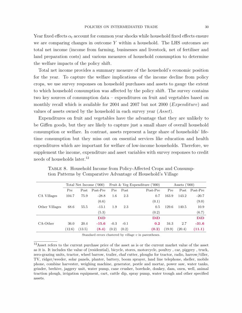
Total net income provides a summary measure of the household’s economic position
for the year. To capture the welfare implications of the income decline from policy
crops, we use survey responses on household purchases and assets to gauge the extent
to which household consumption was affected by the policy shift. The survey contains
two key sources of consumption data – expenditures on fruit and vegetables based on
monthly recall which is available for 2004 and 2007 but not 2000 (Expenditure) and
values of assets owned by the household in each survey year (Asset).
Expenditures on fruit and vegetables have the advantage that they are unlikely to
be Giffen goods, but they are likely to capture just a small share of overall household
consumption or welfare. In contrast, assets represent a large share of households’ life-
time consumption but they miss out on essential services like education and health
expenditures which are important for welfare of low-income households. Therefore, we
supplement the income, expenditure and asset variables with survey responses to credit
needs of households later.12
Table 8. Household Income from Policy-Affected Crops and Consump-tion Patterns by Comparative Advantage of Household’s Village
Total Net Income (’000) Fruit & Veg Expenditure (’000) Assets (’000)
Pre Post Post-Pre Pre Post Post-Pre Pre Post Post-Pre
CA Villages 104.7 75.9 -28.8 1.6 2.3 0.7 163.9 143.2 -20.7
(6.6) (0.1) (9.0)
Other Villages 68.6 55.5 -13.1 1.9 2.3 0.5 129.6 140.5 10.9
(5.3) (0.2) (6.7)
DiD DiD DiD
CA-Other 36.0 20.4 -15.6 -0.3 -0.1 0.2 34.3 2.7 -31.6
(12.6) (13.5) (8.4) (0.2) (0.2) (0.2) (19.9) (20.4) (11.1)
Standard errors clustered by village v in parentheses.
12Asset refers to the current purchase price of the asset as is or the current market value of the assetas it is. It includes the value of (residential), bicycle, stores, motorcycle, poultry , car, piggery , truck,zero-grazing units, tractor, wheel barrow, trailer, chaf cutter, ploughs for tractor, radio, harrow/tiller,TV, ridger/weeder, solar panels, planter, battery, boom sprayer, land line telephone, sheller, mobilephone, combine harvester, weighing machine, generator, pestle and mortar, power saw, water tanks,grinder, beehive, jaggery unit, water pump, cane crusher, borehole, donkey, dam, oxen, well, animaltraction plough, irrigation equipment, cart, cattle dip, spray pump, water trough and other specifiedassets.
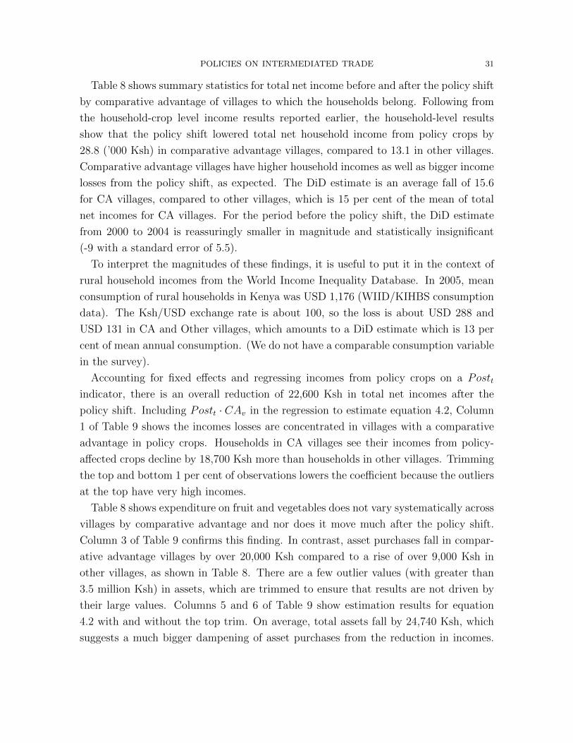
POLICIES ON INTERMEDIATED TRADE 31
Table 8 shows summary statistics for total net income before and after the policy shift
by comparative advantage of villages to which the households belong. Following from
the household-crop level income results reported earlier, the household-level results
show that the policy shift lowered total net household income from policy crops by
28.8 (’000 Ksh) in comparative advantage villages, compared to 13.1 in other villages.
Comparative advantage villages have higher household incomes as well as bigger income
losses from the policy shift, as expected. The DiD estimate is an average fall of 15.6
for CA villages, compared to other villages, which is 15 per cent of the mean of total
net incomes for CA villages. For the period before the policy shift, the DiD estimate
from 2000 to 2004 is reassuringly smaller in magnitude and statistically insignificant
(-9 with a standard error of 5.5).
To interpret the magnitudes of these findings, it is useful to put it in the context of
rural household incomes from the World Income Inequality Database. In 2005, mean
consumption of rural households in Kenya was USD 1,176 (WIID/KIHBS consumption
data). The Ksh/USD exchange rate is about 100, so the loss is about USD 288 and
USD 131 in CA and Other villages, which amounts to a DiD estimate which is 13 per
cent of mean annual consumption. (We do not have a comparable consumption variable
in the survey).
Accounting for fixed effects and regressing incomes from policy crops on a Postt
indicator, there is an overall reduction of 22,600 Ksh in total net incomes after the
policy shift. Including Postt · CAv in the regression to estimate equation 4.2, Column
1 of Table 9 shows the incomes losses are concentrated in villages with a comparative
advantage in policy crops. Households in CA villages see their incomes from policy-
affected crops decline by 18,700 Ksh more than households in other villages. Trimming
the top and bottom 1 per cent of observations lowers the coefficient because the outliers
at the top have very high incomes.
Table 8 shows expenditure on fruit and vegetables does not vary systematically across
villages by comparative advantage and nor does it move much after the policy shift.
Column 3 of Table 9 confirms this finding. In contrast, asset purchases fall in compar-
ative advantage villages by over 20,000 Ksh compared to a rise of over 9,000 Ksh in
other villages, as shown in Table 8. There are a few outlier values (with greater than
3.5 million Ksh) in assets, which are trimmed to ensure that results are not driven by
their large values. Columns 5 and 6 of Table 9 show estimation results for equation
4.2 with and without the top trim. On average, total assets fall by 24,740 Ksh, which
suggests a much bigger dampening of asset purchases from the reduction in incomes.
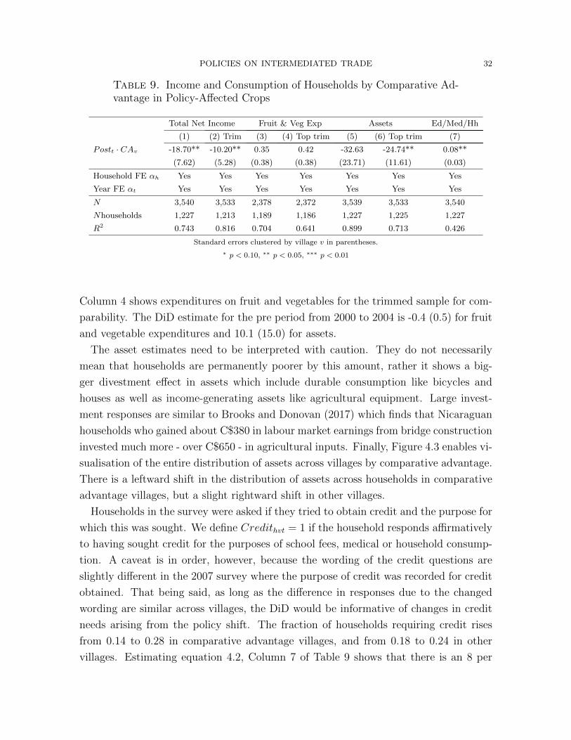
POLICIES ON INTERMEDIATED TRADE 32
Table 9. Income and Consumption of Households by Comparative Ad-vantage in Policy-Affected Crops
Total Net Income Fruit & Veg Exp Assets Ed/Med/Hh
(1) (2) Trim (3) (4) Top trim (5) (6) Top trim (7)
Postt · CAv -18.70** -10.20** 0.35 0.42 -32.63 -24.74** 0.08**
(7.62) (5.28) (0.38) (0.38) (23.71) (11.61) (0.03)
Household FE αh Yes Yes Yes Yes Yes Yes Yes
Year FE αt Yes Yes Yes Yes Yes Yes Yes
N 3,540 3,533 2,378 2,372 3,539 3,533 3,540
Nhouseholds 1,227 1,213 1,189 1,186 1,227 1,225 1,227
R2 0.743 0.816 0.704 0.641 0.899 0.713 0.426
Standard errors clustered by village v in parentheses.
∗ p < 0.10, ∗∗ p < 0.05, ∗∗∗ p < 0.01
Column 4 shows expenditures on fruit and vegetables for the trimmed sample for com-
parability. The DiD estimate for the pre period from 2000 to 2004 is -0.4 (0.5) for fruit
and vegetable expenditures and 10.1 (15.0) for assets.
The asset estimates need to be interpreted with caution. They do not necessarily
mean that households are permanently poorer by this amount, rather it shows a big-
ger divestment effect in assets which include durable consumption like bicycles and
houses as well as income-generating assets like agricultural equipment. Large invest-
ment responses are similar to Brooks and Donovan (2017) which finds that Nicaraguan
households who gained about C$380 in labour market earnings from bridge construction
invested much more - over C$650 - in agricultural inputs. Finally, Figure 4.3 enables vi-
sualisation of the entire distribution of assets across villages by comparative advantage.
There is a leftward shift in the distribution of assets across households in comparative
advantage villages, but a slight rightward shift in other villages.
Households in the survey were asked if they tried to obtain credit and the purpose for
which this was sought. We define Credithvt = 1 if the household responds affirmatively
to having sought credit for the purposes of school fees, medical or household consump-
tion. A caveat is in order, however, because the wording of the credit questions are
slightly different in the 2007 survey where the purpose of credit was recorded for credit
obtained. That being said, as long as the difference in responses due to the changed
wording are similar across villages, the DiD would be informative of changes in credit
needs arising from the policy shift. The fraction of households requiring credit rises
from 0.14 to 0.28 in comparative advantage villages, and from 0.18 to 0.24 in other
villages. Estimating equation 4.2, Column 7 of Table 9 shows that there is an 8 per
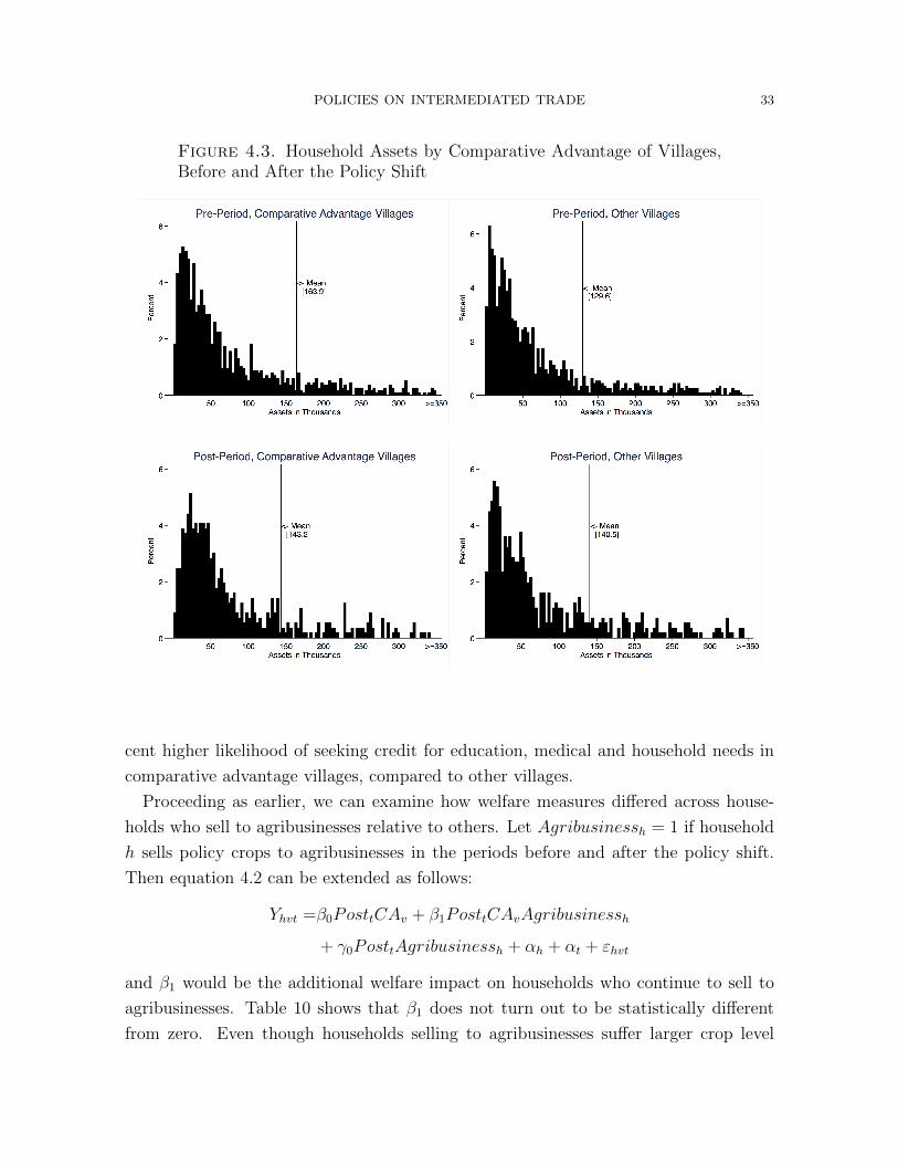
POLICIES ON INTERMEDIATED TRADE 33
Figure 4.3. Household Assets by Comparative Advantage of Villages,Before and After the Policy Shift
cent higher likelihood of seeking credit for education, medical and household needs in
comparative advantage villages, compared to other villages.
Proceeding as earlier, we can examine how welfare measures differed across house-
holds who sell to agribusinesses relative to others. Let Agribusinessh = 1 if household
h sells policy crops to agribusinesses in the periods before and after the policy shift.
Then equation 4.2 can be extended as follows:
Yhvt =β0PosttCAv + β1PosttCAvAgribusinessh
+ γ0PosttAgribusinessh + αh + αt + εhvt
and β1 would be the additional welfare impact on households who continue to sell to
agribusinesses. Table 10 shows that β1 does not turn out to be statistically different
from zero. Even though households selling to agribusinesses suffer larger crop level
POLICIES ON INTERMEDIATED TRADE 34
income losses, they have much higher incomes and other sources of funds so that their
consumption does not suffer much more.
Table 10. Income and Consumption of Households by AgribusinessPurchases and Comparative Advantage
(1) Total Net Income (1) Fruit & Veg (2) Assets (3) Ed/Med/Hh Credit
Postt · CAv -17.56** 0.53 -24.40** 0.07**
(7.93) (0.38) (11.87) (0.04)
Postt · CAv ·Agribusinessh -12.88 -1.11 -17.67 0.08
(21.33) (0.82) (54.48) (0.14)
Postt ·Agribusinessh 11.87 -1.20** -9.63 0.01
(7.39) (0.58) (15.62) (0.07)
Household FE αi Yes Yes Yes Yes
Year FE αt Yes Yes Yes Yes
N 3,540 2,372 3,533 3,540
Nhouseholds 1,227 1,186 1,225 1,227
R2 0.642 0.642 0.713 0.426
Standard errors clustered by village v in parentheses.
∗ p < 0.10, ∗∗ p < 0.05, ∗∗∗ p < 0.01
Summing up, overall household incomes fall more in villages with a comparative
advantage in policy crops. These households are still able to afford similar levels of
their daily food expenditures but their big ticket purchases suffer. The value of the
assets they own falls much more and there is some evidence suggesting that their credit
needs for education, health and household consumption rises. Therefore, many low-
income rural households experience a decline in welfare after the shift in policy to an
agribusiness model in crop markets.
5. Conclusion
Policies to encourage agribusiness-led development of crop markets have often been
proposed as a way of raising agricultural productivity and reducing poverty. A number
of proposals are on the table in several countries to adopt such policies. Yet there is
limited evidence on the impact of these policies on low-income farming households.
Theoretical work has shown that farmers can lose out from policies to promote inter-
mediation when entering intermediaries have greater market power. This paper applies
this insight to policies to promote agribusiness entry into crop markets. Taking the
theory to data from Kenya, the paper shows that Kenyan households experienced a
greater reduction in incomes from crops that saw a shift from state to agribusiness-led
intermediation in farming.
POLICIES ON INTERMEDIATED TRADE 35
As state companies withdrew from intermediation to make way for agribusinesses,
profit margins of agribusiness firms specialising in the policy-affected crops grew much
more than those of firms specialising in other crops. Despite policies to increase compe-
tition, large agribusiness firms that specialised in the policy crops saw a 5 to 8 per cent
greater increase in their profit margins. The policy shift therefore raised firm profits at
the expense of farm incomes for households.
Overall incomes and consumption of households fell, and the income losses were con-
centrated in villages specialising in the policy-affected crops (owing to greater compara-
tive advantage from agroecological factors). Households in villages with a comparative
advantage in policy-affected crops saw bigger overall income losses, with the difference
being equivalent to 13 per cent of average annual consumption of rural households in
Kenya. These households adjusted to the income loss by drawing down on the value of
the assets that they owned.
To sum up, the results provide evidence for long-standing concerns in the literature
that commercialisation of agriculture, via agribusinesses that wield monopsony power,
need not raise income earning opportunities for small farmers. The results also confirm
the lesson taken by the Kenyan government from this experience. In the revised version
of their agricultural strategy in 2010, policymakers reflected on how smallholder farmers
could suffer when “liberalisation is carried out where there is no critical mass and enough
capacity for the private sector to grow” (ASDS 2010). As long panels start to evolve,
further work can provide a better understanding of the conditions that can enable
agribusiness intermediation to translate into productivity gains for low-income farmers.
References
ASDS, “Agricultural Sector Development Strategy 2010–2020,” Government of Kenya,
2010.
Allen, Treb and David Atkin, “Volatility and the Gains from Trade,” Technical Report,
National Bureau of Economic Research 2016.
Antras, Pol and Arnaud Costinot, “Intermediated Trade,” The Quarterly Journal of
Economics, 2011, 126 (3), 1319–1374.
Atkin, David and Dave Donaldson, “Who’s getting globalized? the size and nature of
intranational trade costs,” Yale University and MIT, unpublished mimeo, 2012.
Bardhan, Pranab, Dilip Mookherjee, and Masatoshi Tsumagari, “Middlemen margins
and globalization,” American Economic Journal: Microeconomics, 2013, 5 (4), 81–119.
Barrett, Christopher B., “Smallholder market participation: Concepts and evidence
from eastern and southern Africa,” Food Policy, 2008, 33 (4), 299–317.
POLICIES ON INTERMEDIATED TRADE 36
Barrett, Christopher B. and Emelly Mutambatsere, Agricultural markets in developing
countries, Vol. 2nd Edition, London: Palgrave Macmillan, 2008.
Bergquist, Lauren F. and Michael Dinerstein, “Competition and Entry in Agricultural
Markets: Experimental Evidence from Kenya,” Working Paper, 2019.
Bhagwati, Jagdish N., Arvind Panagariya, and Thirukodikaval N. Srinivasan, Lectures
on international trade, MIT press, 1998.
Brambilla, Irene and Guido G. Porto, “Market structure, outgrower contracts, and farm
output. Evidence from cotton reforms in Zambia,” Oxford Economic Papers, 2011.
Brooks, Wyatt and Kevin Donovan, “Eliminating Uncertainty in Market Access: The
Impact of New Bridges in Rural Nicaragua,” Working Paper, 2017.
Carr, Stephen, “What happens to the small farmers when the large ones take over?,”
Thrive, CGIAR Research Program on Water, Land and Ecosystems, February 2013.
Casaburi, Lorenzo and Tristan Reed, “Competition in Agricultural Markets: An Ex-
perimental Approach,” CEPR Discussion Paper No. DP11985, 2017.
Chamberlin, Jordan and T. S. Jayne, “Unpacking the meaning of ’market access’: evi-
dence from rural Kenya,” World Development, 2013, 41, 245–264.
Chatterjee, Shoumitro, “Market Power and Spatial Competition in Rural India,” Work-
ing Paper, 2019.
Chau, Nancy, Hideaki Goto, and Ravi Kanbur, “Middlemen, Non-Profits, and Poverty,”
Technical Report, Cornell University, Department of Applied Economics and Manage-
ment 2009.
Collier, Paul and Stefan Dercon, “African Agriculture in 50Years: Smallholders in a
Rapidly Changing World?,” World Development, 2014, 63, 92–101.
Conley, Timothy G. and Christopher R. Udry, “Learning about a new technology:
Pineapple in Ghana,” The American Economic Review, 2010, 100 (1), 35–69.
Devadoss, Stephen and Wongun Song, “Oligopsony Distortions and Welfare Implica-
tions of Trade,” Review of International Economics, 2006, 14 (3), 452–465.
Dhingra, Swati and Silvana Tenreyro, “Piggy-Back Exporting, Intermediation, and the
Gains from Trade to Small Farmers,” Working Paper, 2017.
Dillon, Brian and Chelsey Dambro, “How Competitive Are Crop Markets in Sub-
Saharan Africa?,” American Journal of Agricultural Economics, 2017, 99 (5), 1344-
1361.
Fafchamps, Marcel and Ruth V. Hill, “Price transmission and trader entry in domestic
commodity markets,” Economic Development and Cultural Change, 2008, 56 (4), 729–
766.
POLICIES ON INTERMEDIATED TRADE 37
FAOSTAT, “Review of food and agricultural policies in the Kenya 2005-2011,” Country
Report, February 2013.
Feenstra, Robert C., “Monopsony distortions in an open economy: A theoretical anal-
ysis,” Journal of International Economics, 1980, 10 (2), 213–235.
Goodman, David and Michael Watts, Globalising food: agrarian questions and global
restructuring, Psychology Press, 1997.
Grant, Matthew and Meredith Startz, “Cutting Out the Middleman: The Structure of
Chains of Intermediation” Working Paper, January 2019.
Lagakos, David and Michael E. Waugh, “Selection, agriculture, and cross-country pro-
ductivity differences,” The American Economic Review, 2013, 103 (2), 948–980.
Lowder, Sarah K., Jakob Skoet, and Saumya Singh, “What do we really know about
the number and distribution of farms and family farms in the world?,” FAO, 2014.
Macchiavello, Rocco and Ameet Morjaria, “The value of relationships: evidence from
a supply shock to Kenyan rose exports,” The American Economic Review, 2015, 105
(9), 2911–2945.
Macchiavello, Rocco and Ameet Morjaria, “Competition and Relational Contracts: Ev-
idence from Rwanda’s Coffee Mills,” Technical Report, Working Paper, LSE and Har-
vard 2015.
Markusen, James R. and Arthur J. Robson, “Simple general equilibrium and trade with
a monopsonized sector,” Canadian Journal of Economics, 1980, pp. 668–682.
McCulloch, Rachel and Janet L. Yellen, “Factor market monopsony and the allocation
of resources,” Journal of International Economics, 1980, 10 (2), 237–247.
Minot, Nicholas, “Contract farming in sub-Saharan Africa: opportunities and chal-
lenges,” in “Policy seminar: Smallholder-led Agricultural Commercialization and Poverty
Reduction: How to Achieve It,” 2011, pp. 18–22.
Minten, Bart, Lalaina Randrianarison, and Johan F. M. Swinnen, “Global retail chains
and poor farmers: Evidence from Madagascar,” World Development, 2009, 37 (11),
1728–1741.
Nunn, Nathan and Nancy Qian, “The Potato’s Contribution to Population and Urban-
ization: Evidence from a Historical Experiment,” The Quarterly Journal of Economics,
2011, 126 (2), 593-650.
Poulton, Colin and Karuti Kanyinga, “The Politics of Revitalising Agriculture in Kenya,”
Development Policy Review, 2014, 32 (S2), s151-s172.
Provost, C. and E. Kabendera, “Tanzania: ’large-scale farming turns small farmers into
mere labourers’,” The Guardian, February 2014.
POLICIES ON INTERMEDIATED TRADE 38
Provost, C., L. Ford, and M. Tran, “New Alliance condemned as new wave of colonialism
in Africa,” The Guardian, February 2014.
Reardon, Thomas and C. Peter Timmer, “Transformation of markets for agricultural
output in developing countries since 1950: How has thinking changed?,” Handbook of
Agricultural Economics, 2007, 3, 2807–2855.
Robbins, Peter and R. S. B. Ferris, The impact of globalization on the agricultural
sectors of East and Central African countries, Vol. 1, Iita, 2003.
Runsten, David, “Transaction Costs in Mexican Fruit and Vegetable Contracting: Im-
plications for Asociacion en participacipation,” Atlanta, 1994, 10, 12.
Sheveleva, Yelena and Kala Krishna, “Wheat or Strawberries? Intermediated Trade
with Limited Contracting,” American Economic Journal: Microeconomics, 2016.
Startz, Meredith, “The value of face-to-face: Search and contracting problems in Nige-
rian trade,” Working Paper, 2018.
Suri, Tavneet, “Selection and Comparative Advantage in Technology Adoption,” Econo-
metrica, 2011, 79 (1), 159–209.
Suri, Tavneet, David Tschirley, Charity Irungu, Raphael Gitau, Daniel Kariuki, and
Others, “Rural incomes, inequality and poverty dynamics in Kenya”, Egerton univer-
sity. Tegemeo institute of agricultural policy and development, 2009.
Tomar, Shekhar, “Gains from Agricultural Market Integration: Role and Size of Inter-
mediaries,” Working Paper, 2009.
UNCTAD, “World Investment Report 2009: Transnational Corporations, Agricultural
Production and Development,” 2009.
Warning, Matthew and Nigel Key, “The social performance and distributional con-
sequences of contract farming: An equilibrium analysis of the Arachide de Bouche
program in Senegal,” World Development, 2002, 30 (2), 255–263.
Winter-Nelson, Alex and Gem Argwings-Kodhek, “Distortions to Agricultural Incen-
tives in Kenya,” Agricultural Distortions Working Paper 45, December 2007.
Appendix
Equilibrium. To ensure that there is more than one entrant in the market for policy
crops, we make the following assumption in terms of primitives:
Assumption: Entry costs are low enough for at least one firm to enter. Specifically,
N ≥ 1 if Fkk−1/ (k − 1)k−2 ≤ ((1− κ) pm+ κps)k ϕkmin.
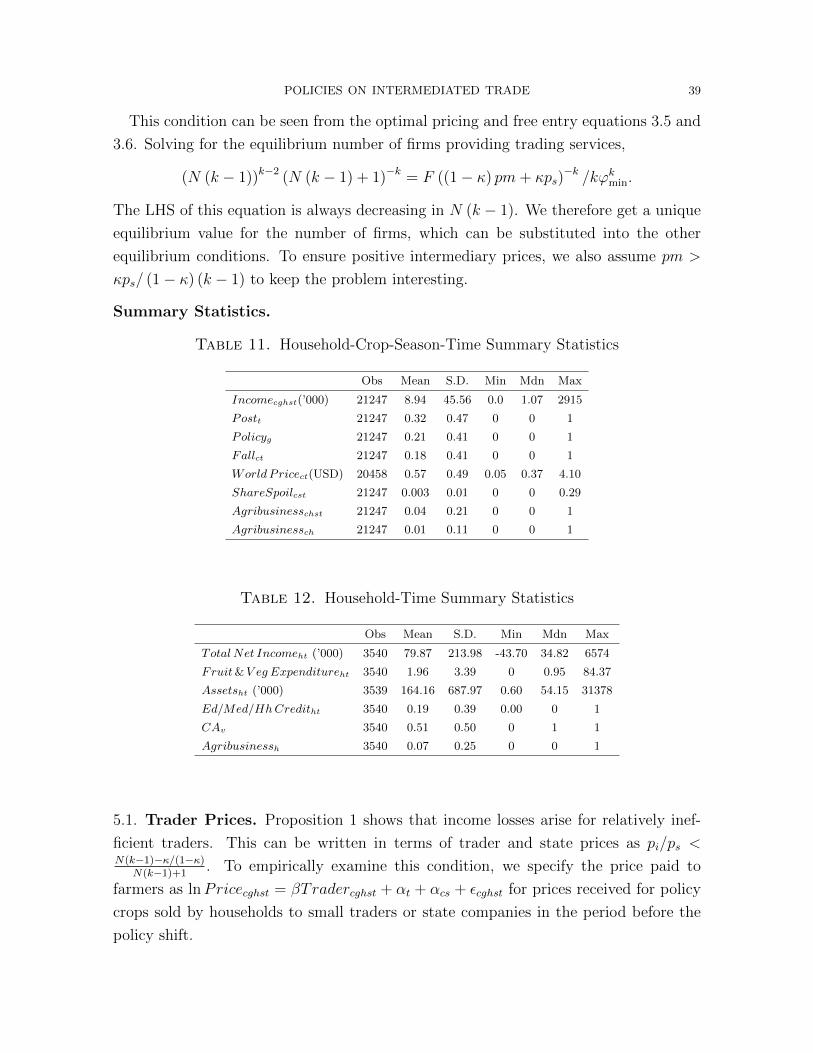
POLICIES ON INTERMEDIATED TRADE 39
This condition can be seen from the optimal pricing and free entry equations 3.5 and
3.6. Solving for the equilibrium number of firms providing trading services,
(N (k − 1))k−2 (N (k − 1) + 1)−k = F ((1− κ) pm+ κps)−k /kϕkmin.
The LHS of this equation is always decreasing in N (k − 1). We therefore get a unique
equilibrium value for the number of firms, which can be substituted into the other
equilibrium conditions. To ensure positive intermediary prices, we also assume pm >
κps/ (1− κ) (k − 1) to keep the problem interesting.
Summary Statistics.
Table 11. Household-Crop-Season-Time Summary Statistics
Obs Mean S.D. Min Mdn Max
Incomecghst(’000) 21247 8.94 45.56 0.0 1.07 2915
Postt 21247 0.32 0.47 0 0 1
Policyg 21247 0.21 0.41 0 0 1
Fallct 21247 0.18 0.41 0 0 1
WorldPricect(USD) 20458 0.57 0.49 0.05 0.37 4.10
ShareSpoilcst 21247 0.003 0.01 0 0 0.29
Agribusinesschst 21247 0.04 0.21 0 0 1
Agribusinessch 21247 0.01 0.11 0 0 1
Table 12. Household-Time Summary Statistics
Obs Mean S.D. Min Mdn Max
Total Net Incomeht (’000) 3540 79.87 213.98 -43.70 34.82 6574
Fruit&V eg Expenditureht 3540 1.96 3.39 0 0.95 84.37
Assetsht (’000) 3539 164.16 687.97 0.60 54.15 31378
Ed/Med/HhCreditht 3540 0.19 0.39 0.00 0 1
CAv 3540 0.51 0.50 0 1 1
Agribusinessh 3540 0.07 0.25 0 0 1
5.1. Trader Prices. Proposition 1 shows that income losses arise for relatively inef-
ficient traders. This can be written in terms of trader and state prices as pi/ps <N(k−1)−κ/(1−κ)
N(k−1)+1. To empirically examine this condition, we specify the price paid to
farmers as lnPricecghst = βTradercghst + αt + αcs + εcghst for prices received for policy
crops sold by households to small traders or state companies in the period before the
policy shift.
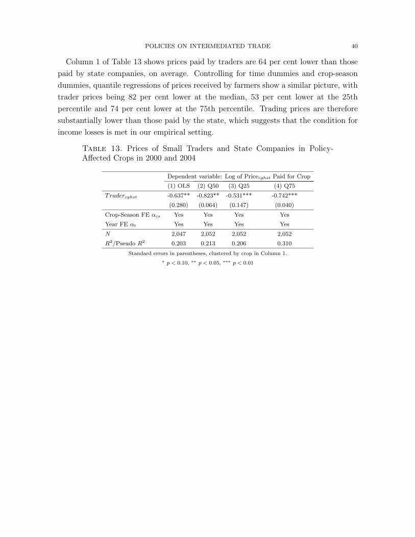
POLICIES ON INTERMEDIATED TRADE 40
Column 1 of Table 13 shows prices paid by traders are 64 per cent lower than those
paid by state companies, on average. Controlling for time dummies and crop-season
dummies, quantile regressions of prices received by farmers show a similar picture, with
trader prices being 82 per cent lower at the median, 53 per cent lower at the 25th
percentile and 74 per cent lower at the 75th percentile. Trading prices are therefore
substantially lower than those paid by the state, which suggests that the condition for
income losses is met in our empirical setting.
Table 13. Prices of Small Traders and State Companies in Policy-Affected Crops in 2000 and 2004
Dependent variable: Log of Pricecghst Paid for Crop
(1) OLS (2) Q50 (3) Q25 (4) Q75
Tradercghst -0.637** -0.823** -0.531*** -0.742***
(0.280) (0.064) (0.147) (0.040)
Crop-Season FE αcs Yes Yes Yes Yes
Year FE αt Yes Yes Yes Yes
N 2,047 2,052 2,052 2,052
R2/Pseudo R2 0.203 0.213 0.206 0.310
Standard errors in parentheses, clustered by crop in Column 1.
∗ p < 0.10, ∗∗ p < 0.05, ∗∗∗ p < 0.01

CENTRE FOR ECONOMIC PERFORMANCE Recent Discussion Papers
1676 Jeffrey Grogger Ria Ivandic Tom Kirchmaier
Comparing Conventional and Machine-Learning Approaches to Risk Assessment in Domestic Abuse Cases
1675 Mary Amiti Stephen J. Redding David E. Weinstein
Who’s Paying for the U.S. Tariffs? A Longer-Term Perspective
1674 Cheng Chen Claudia Steinwender
Import Competition, Heterogeneous Preferences of Managers and Productivity
1673 Stefano Bolatto Alireza Naghavi Gianmarco Ottaviano Katja Zajc Kejzar
Intellectual Property and the Organization of the Global Value Chain
1672 Timothy Besley Isabel Roland John Van Reenen
The Aggregate Consequences of Default Risk: Evidence from Firm-Level Data
1671 Jan-Emmanuel De Neve Daisy Fancourt Christian Krekel Richard Layard
A Local Community Course That Raises Mental Wellbeing and Pro-Sociality
1670 Tommaso Sonno Globalization and Conflicts: The Good, the Bad and the Ugly of Corporations in Africa
1669 Michael Amior Immigration, Local Crowd-Out and Undercoverage Bias
1668 Antoine Berthou John Jong-Hyun Chung Kalina Manova Charlotte Sandoz Dit Bragard
Trade, Productivity and (Mis)allocation

1667 Holger Breinlich Elsa Leromain Dennis Novy Thomas Sampson
Exchange Rates and Consumer Prices: Evidence from Brexit
1666 Fabrice Defever Michele Imbruno Richard Kneller
Trade Liberalization, Input Intermediaries and Firm Productivity: Evidence from China
1665 Philippe Aghion Antonin Bergeaud Richard Blundell Rachel Griffith
The Innovation Premium to Soft Skills in Low-Skilled Occupations
1664 Filip Gesiarz Jan-Emmanuel De Neve Tali Sharot
The Motivational Cost of Inequality: Pay Gaps Reduce the Willingness to Pursue Rewards
1663 Felix Koenig Technical Change and Superstar Effects: Evidence From the Roll-Out of Television
1662 Enrico Moretti Claudia Steinwender John Van Reenen
The Intellectual Spoils of War? Defense R&D, Productivity and International Spillovers
1661 Decio Coviello Andrea Ichino Nicola Persico
Measuring the Gains from Labor Specialization
1660 Nicolás González-Pampillón Spillover Effects from New Housing Supply
1659 Walter Bossert Andrew E. Clark Conchita D’Ambrosio Anthony Lepinteur
Economic Insecurity and the Rise of the Right
The Centre for Economic Performance Publications Unit Tel: +44 (0)20 7955 7673 Email [email protected] Website: http://cep.lse.ac.uk Twitter: @CEP_LSE