ISSN 2042-2695

CEP Discussion Paper No 1229

July 2013

Unmet Aspirations as an Explanation for the

Age U-shape in Human Wellbeing

Hannes Schwandt

Abstract A large literature in behavioral and social sciences has found that human wellbeing follows a

U-shape over age. Some theories have assumed that the U-shape is caused by unmet

expectations that are felt painfully in midlife but beneficially abandoned and experienced

with less regret during old age. In a unique panel of 132,609 life satisfaction expectations

matched to subsequent realizations, I find people to err systematically in predicting their life

satisfaction over the life cycle. They expect -- incorrectly -- increases in young adulthood

and decreases during old age. These errors are large, ranging from 9.8% at age 21 to -4.5% at

age 68, they are stable over time and observed across socio-economic groups. These findings

support theories that unmet expectations drive the age U-shape in wellbeing.

.

JEL Classifications: A12, I30, D84

Keywords: life satisfaction, expectations, aging

This paper was produced as part of the Centre’s Wellbeing Programme. The Centre for

Economic Performance is financed by the Economic and Social Research Council.

Acknowledgements I am thankful to Ada Ferrer-i-Carbonell, Robin Hogarth and Andrew Oswald for guidance

and advice on this project as well as to Janet Currie, Guy Mayraz, Johannes Müller-Trede,

Hannes Wiese and Tali Sharot for helpful comments.

Hannes Schwandt is a Visiting Research Scholar with the Centre for Economic

Performance, London School of Economics and Political Science. He is also a Postdoctoral

Research Associate at the Center for Health and Wellbeing, Woodrow Wilson School,

Princeton University.

Published by

Centre for Economic Performance

London School of Economics and Political Science

Houghton Street

London WC2A 2AE

All rights reserved. No part of this publication may be reproduced, stored in a retrieval

system or transmitted in any form or by any means without the prior permission in writing of

the publisher nor be issued to the public or circulated in any form other than that in which it

is published.

Requests for permission to reproduce any article or part of the Working Paper should be sent

to the editor at the above address.

H. Schwandt, submitted 2013

2

1. Introduction

Behavioral and social scientists have shown increasing interest in self-reported life

satisfaction and other subjective indicators as measures of human wellbeing (1-3). Using

these measures a large and emerging literature has established that wellbeing follows a U-

shape over age (4-8). Even though some controversy remains over the existence of this U-

shape (9), it has been observed in over 50 nations (4), across socio-economic groups (5)

and recently also for great apes (7). Little is known about its origins (7). One theory (8) is

that the U-shape is driven by unmet aspirations which are painfully felt in midlife but

beneficially abandoned later in life. A complementary theory builds on the neuroscientific

finding (10) that the emotional reaction to missed chances decreases with age so that the

elderly might feel less regret about unmet aspirations.

Assuming that regret about unmet aspirations drives the U-shape implies that

people err dramatically in predicting their wellbeing over the life-cycle. When young,

people expect a bright future though actual wellbeing decreases. In old age expectations

are adjusted downwards though actual wellbeing is rising. Human belief formation is

known to exhibit systematic biases such as optimism (11-15) and the underestimation of

hedonic adaptation to changes in life circumstances (16, 17). However, existing literatures

typically analyze specific forecast settings with less emphasis on overall wellbeing

measures or the role of age. The extent to which people err in predicting changes in their

wellbeing over the life-cycle is unknown.

This paper examines whether people make systematic errors when thinking about

their wellbeing in five years time and how these errors change with age. Results are based

on a unique data set from the German Socio-Economic Panel (SOEP) that includes both

respondents' current life satisfaction as well as their expectations about life satisfaction in

five years. The panel structure of the SOEP allows an individual's expectation in a given

year to be matched to the same individual's realization five years ahead to form individual

specific forecast errors..

The SOEP is a representative annual survey that started in West-Germany in 1984

and includes East-Germany since 1990. Current life satisfaction is reported in all years

3

while expected life satisfaction is included from 1991 to 2004. The wording of the

questions, translated from German, is:

Please answer according to the following scale: 0 means 'completely dissatisfied', 10 means 'completely satisfied':

- How satisfied are you with your life, all things considered? [1]

- And how do you think you will feel in five years? [2]

It is important to distinguish self-reported life satisfaction from other subjective

wellbeing measures (18). For example, the findings of this paper might not carry over to

reports of momentary emotional affect. However, life satisfaction might be of particular

interest in the context of wellbeing forecasts. Recent experimental evidence (19) indicates

that people tend to choose those life circumstances for which they predict the highest

future life satisfaction rather than the most pleasant future hedonic experience.

2. Results

The sample used in this study is all those respondents between the ages of 17 and 85 who

responded to question [2] in the waves 1991 to 2002 and to question [1] five years later.

The resulting sample consists of 23,161 individuals for whom a total of 132,609 life

satisfaction forecast errors were constructed. Descriptive statistics are provided in Table

A1.

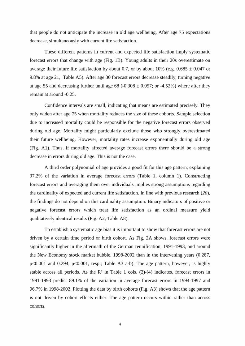
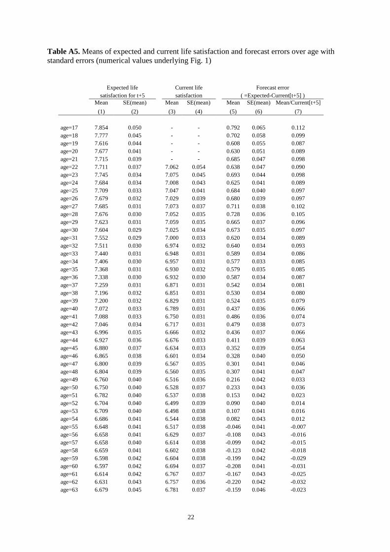
Figure 1A plots people's expected life satisfaction in five years averaged over age

at the forecast, ranging from age 17 to 85, and the same sample's current life satisfaction

five years ahead at ages 22 to 90. In line with the existing literature (4-8) current life

satisfaction is U-shaped between ages 20 and 70, with peaks around ages 23 and 69, a

local minimum in the mid-50s and a further decline after age 75. As the plot of life

satisfaction expectations shows, this U-shape is not anticipated. During young adulthood

people expect their life satisfaction to increase strongly. With age, expectations decrease

but remain above current life satisfaction until the late 50s when the two graphs coincide.

Thereafter expectations remain stable while actual life satisfaction increases, indicating

4

that people do not anticipate the increase in old age wellbeing. After age 75 expectations

decrease, simultaneously with current life satisfaction.

These different patterns in current and expected life satisfaction imply systematic

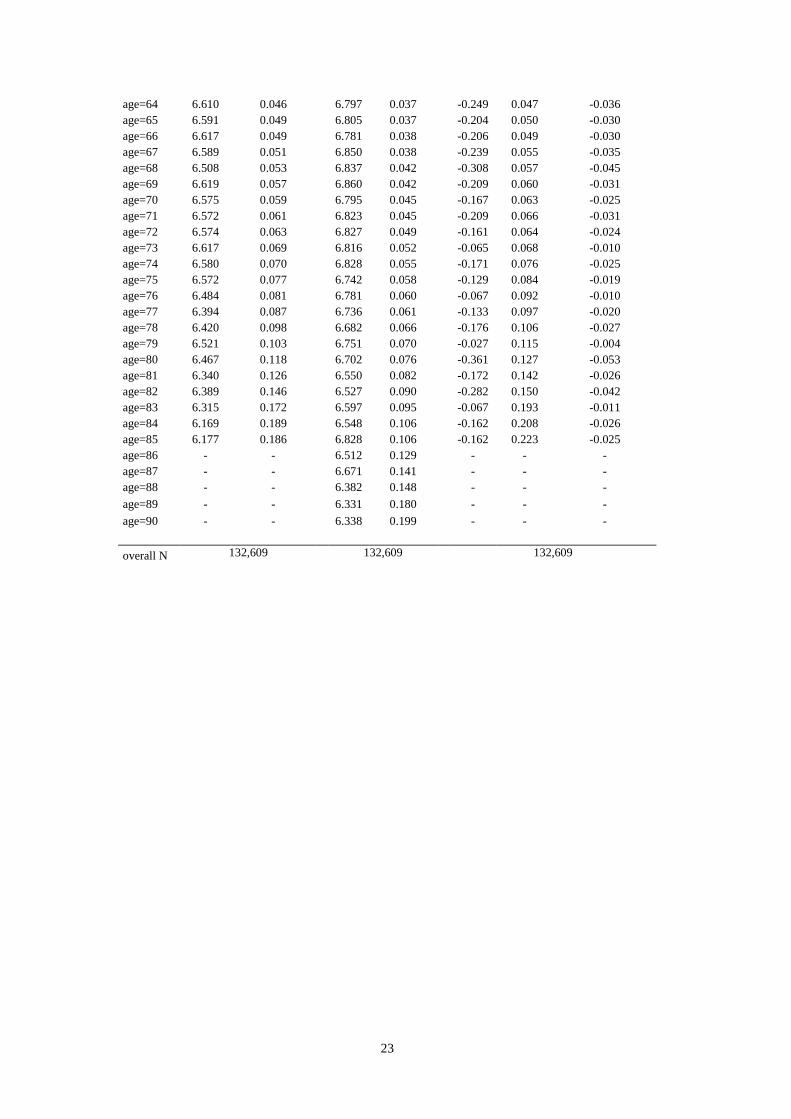
forecast errors that change with age (Fig. 1B). Young adults in their 20s overestimate on

average their future life satisfaction by about 0.7, or by about 10% (e.g. 0.685 ± 0.047 or

9.8% at age 21, Table A5). After age 30 forecast errors decrease steadily, turning negative

at age 55 and decreasing further until age 68 (-0.308 ± 0.057; or -4.52%) where after they

remain at around -0.25.

Confidence intervals are small, indicating that means are estimated precisely. They

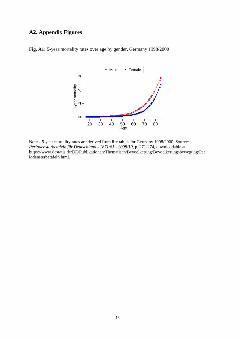
only widen after age 75 when mortality reduces the size of these cohorts. Sample selection

due to increased mortality could be responsible for the negative forecast errors observed

during old age. Mortality might particularly exclude those who strongly overestimated

their future wellbeing. However, mortality rates increase exponentially during old age

(Fig. A1). Thus, if mortality affected average forecast errors there should be a strong

decrease in errors during old age. This is not the case.

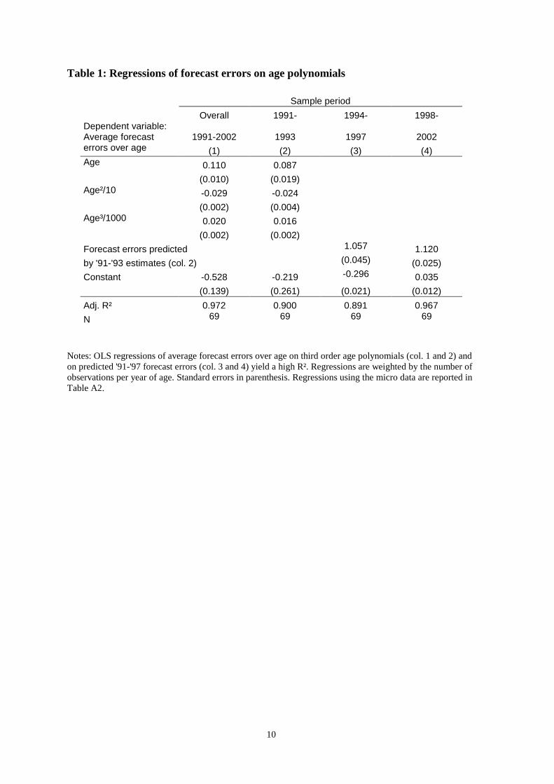
A third order polynomial of age provides a good fit for this age pattern, explaining

97.2% of the variation in average forecast errors (Table 1, column 1). Constructing

forecast errors and averaging them over individuals implies strong assumptions regarding

the cardinality of expected and current life satisfaction. In line with previous research (20),

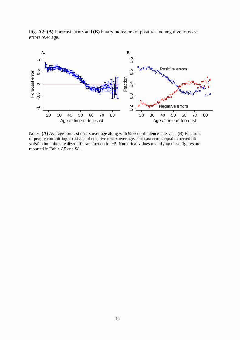
the findings do not depend on this cardinality assumption. Binary indicators of positive or

negative forecast errors which treat life satisfaction as an ordinal measure yield

qualitatively identical results (Fig. A2, Table A8).

To establish a systematic age bias it is important to show that forecast errors are not

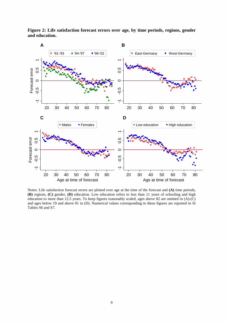
driven by a certain time period or birth cohort. As Fig. 2A shows, forecast errors were

significantly higher in the aftermath of the German reunification, 1991-1993, and around

the New Economy stock market bubble, 1998-2002 than in the intervening years (0.287,

p<0.001 and 0.294, p<0.001, resp.; Table A3 a-b). The age pattern, however, is highly

stable across all periods. As the R² in Table 1 cols. (2)-(4) indicates. forecast errors in

1991-1993 predict 89.1% of the variation in average forecast errors in 1994-1997 and

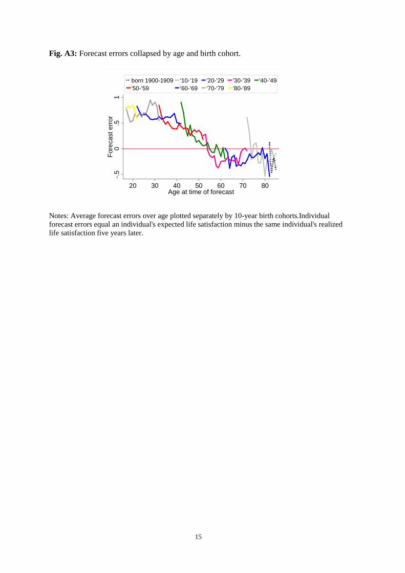
96.7% in 1998-2002. Plotting the data by birth cohorts (Fig. A3) shows that the age pattern

is not driven by cohort effects either. The age pattern occurs within rather than across

cohorts.

5

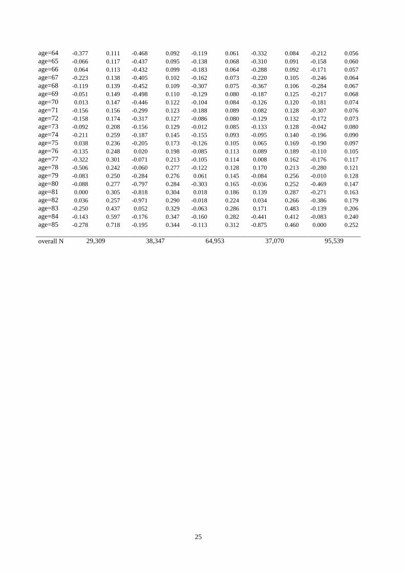
Figure 2B plots forecast errors over the life-cycle separately for East- and West-

Germany. The pattern looks remarkably similar across these two regions that were

economically and culturally different in the aftermath of German Reunification (21).

Below age 55, forecast errors are not significantly different between regions, and only

slightly more negative in East Germany above age 55 (-0.088, p<0.001, Table A3 c-d). As

shown in Fig. 2C age effects are also similar by gender. Below age 55, the gender

difference is small and insignificant, while forecast errors are slightly more negative for

males above age 55 (-0.044, p=0.044, Table A3 e-f).

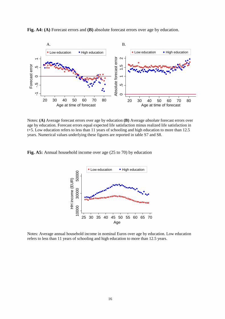
Surprisingly, the life-cycle pattern is more pronounced for the more educated (Fig.

2 D). People with fewer years of education make significantly less positive forecast errors

before age 55 (difference -0.116, p<0.001, Table A3 g) and significantly less negative

forecast errors after age 55 (difference 0.166, p<0.001, Table A3 h). Notice, however, that

smaller average forecast errors do not necessarily imply greater precision. On average,

negative and positive errors cancel out. Average absolute forecast errors are significantly

larger for the less educated (0.226, p<0.001; Table A4, Fig. A4).

3. Discussion

These findings show a striking age-associated bias in life satisfaction forecasts. The young

strongly overestimate their future life satisfaction while the elderly tend to underestimate

it. The similarity of the observed patterns across regions and their stability over time

indicate that the findings might be generalizable to other developed countries in other

decades. Indeed, as Easterlin (22) has shown in a pioneering study, suggestive cross-

sectional evidence on life ladder ranking expectations from the Cantril surveys (23) is in

line with similar age biases in West-Germany and other developed countries around 1960

(see SI Fig. A6).

What are the causes underlying this age bias? One well known source of systematic

forecast errors is that people underestimate how quickly they adapt to socio-economic

changes such as changes in income (16, 17). Thus the observed age bias could be

generated by the young expecting too much from anticipated income increases with the

6

elderly, who face decreasing incomes, committing the opposite error. In the data, forecast

errors indeed roughly match with the average income profile which is increasing during

young adulthood and decreasing after age 50 (Fig. A5). Further, the age bias is slightly

more pronounced for the highly educated who have steeper income profiles than those

with less education (Fig. A5).

However, the remarkable similarity across economically and culturally distinct

regions and across gender suggests that some of the causes of the age bias go beyond age-

related socio-economic characteristics. It is well established finding in psychological

research that people tend to overestimate the likelihood of positive events and

underestimate the likelihood of negative events (11-15, 24). For example, people expect to

enjoy healthier lives than average or underestimate the probability of being divorced (11).

Optimism bias has also been demonstrated in non-human animals (25). Neuroscientific

research (13-15) has accumulated broad evidence that this bias is generated by selective

processing of negative and positive information in the frontal brain which allows people to

maintain biased expectations when confronted with discomforting evidence. This might

provide a biological explanation for why life satisfaction expectations are overoptimistic

during much of adulthood and adjust only slowly over time. It does not explain, though,

why expectations remain stable after midlife while actual life satisfaction increases,

implying negative forecast errors during old age. However, little is known about optimism

in old age and existing evidence is conflicting (26).

How do the age associated errors in expected life satisfaction documented here

relate to the age U-shape in wellbeing? Some theories (8, 10) have assumed that the U-

shape is driven by unmet expectations that negatively affect people's wellbeing in midlife

but are abandoned and experienced with less regret during old age. The data reported here

support this notion. Young adults have high aspirations that are subsequently unmet. And

their life satisfaction decreases with age as long as expectations remain high and unmet.

Aspirations are abandoned and expectations align with current wellbeing in the late 50s.

This is the age when wellbeing starts to rise again. Further, given the disappointed

expectations accumulated until that age, it is possible that wellbeing increases if the elderly

learn to feel less regret (10). Following this interpretation of the U-shape in wellbeing, the

observed negative forecast errors during old age might indicate that people do not

7

anticipate the wellbeing enhancing effects of abandoning high aspirations and

experiencing less regret.

Disseminating the knowledge of age associated forecast errors in life satisfaction

could help people adjust their expectations, optimize important decisions in their life and

suffer less when aspirations are not met. This might weaken the midlife drop in life

satisfaction.

8

4. Figures and Tables

Figure 1: Expected life satisfaction, current life satisfaction and life satisfaction forecast errors over age A B

Notes: Expected life satisfaction, current life satisfaction and life satisfaction forecast errors are plotted over age. (A) (o) Expectations about life satisfaction in five years averaged over age, ranging from age 17 to 85. Sample size is 132,609. (■) The same sample's average current life satisfaction at ages 22 to 90. Current and expected life satisfaction are coded for each individual from a scale of 0 (completely dissatisfied) to 10 (completely satisfied). (B) Individual forecast errors averaged over age at time of the forecast (●) with 95% confidence intervals (I), for the same sample as in (A). Individual forecast errors equal an individual's expected life satisfaction in five years minus the same person's current life satisfaction five years ahead. Numerical values corresponding to both figures are reported in Table A3.

Expected for t+5

Current

66.

57

7.5

8

20 30 40 50 60 70 80 90

Life

sat

isfa

ctio

n

Age

-1-0

.50

0.5

120 30 40 50 60 70 80

For

ecas

t err

or

Age at time of forecast

9

Figure 2: Life satisfaction forecast errors over age, by time periods, regions, gender and education. A B

C D

Notes: Life satisfaction forecast errors are plotted over age at the time of the forecast and (A) time periods, (B) regions, (C) gender, (D) education. Low education refers to less than 11 years of schooling and high education to more than 12.5 years. To keep figures reasonably scaled, ages above 82 are omitted in (A)-(C) and ages below 19 and above 81 in (D). Numerical values corresponding to these figures are reported in SI Tables S6 and S7.

-1-0

.50

0.5

1

20 30 40 50 60 70 80

'91-'93 '94-'97 '98-'02

For

ecas

t err

or

-1-0

.50

0.5

1

20 30 40 50 60 70 80

East-Germany West-Germany

-1-0

.50

0.5

1

20 30 40 50 60 70 80

Males Females

For

ecas

t err

or

Age at time of forecast

-1-0

.50

0.5

1

20 30 40 50 60 70 80

Low education High education

Age at time of forecast

10

Table 1: Regressions of forecast errors on age polynomials

Sample period

Overall 1991- 1994- 1998- Dependent variable: Average forecast 1991-2002 1993 1997 2002 errors over age (1) (2) (3) (4) Age 0.110 0.087

(0.010) (0.019)

Age²/10 -0.029 -0.024

(0.002) (0.004)

Age³/1000 0.020 0.016

(0.002) (0.002)

Forecast errors predicted 1.057 1.120

by '91-'93 estimates (col. 2) (0.045) (0.025)

Constant -0.528 -0.219 -0.296 0.035

(0.139) (0.261) (0.021) (0.012)

Adj. R² 0.972 0.900 0.891 0.967

N 69 69 69 69

Notes: OLS regressions of average forecast errors over age on third order age polynomials (col. 1 and 2) and on predicted '91-'97 forecast errors (col. 3 and 4) yield a high R². Regressions are weighted by the number of observations per year of age. Standard errors in parenthesis. Regressions using the micro data are reported in Table A2.

11

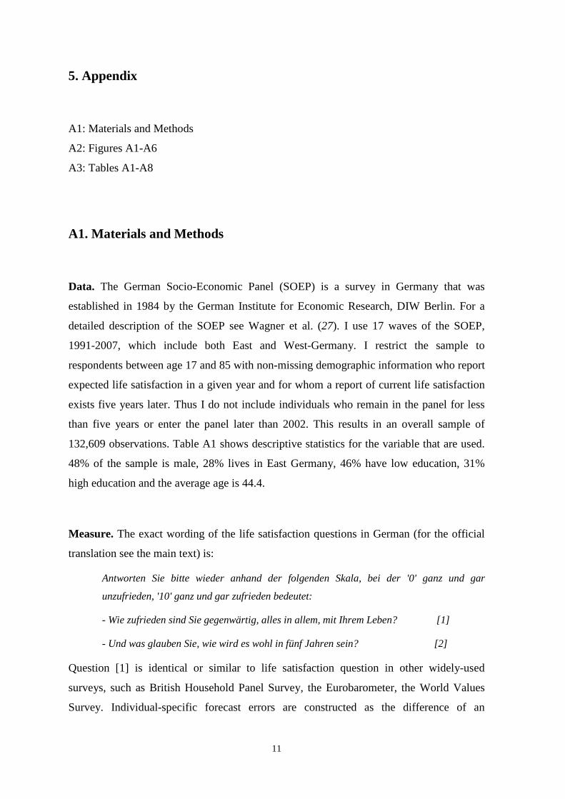
5. Appendix

A1: Materials and Methods

A2: Figures A1-A6

A3: Tables A1-A8

A1. Materials and Methods

Data. The German Socio-Economic Panel (SOEP) is a survey in Germany that was

established in 1984 by the German Institute for Economic Research, DIW Berlin. For a

detailed description of the SOEP see Wagner et al. (27). I use 17 waves of the SOEP,

1991-2007, which include both East and West-Germany. I restrict the sample to

respondents between age 17 and 85 with non-missing demographic information who report

expected life satisfaction in a given year and for whom a report of current life satisfaction

exists five years later. Thus I do not include individuals who remain in the panel for less

than five years or enter the panel later than 2002. This results in an overall sample of

132,609 observations. Table A1 shows descriptive statistics for the variable that are used.

48% of the sample is male, 28% lives in East Germany, 46% have low education, 31%

high education and the average age is 44.4.

Measure. The exact wording of the life satisfaction questions in German (for the official

translation see the main text) is:

Antworten Sie bitte wieder anhand der folgenden Skala, bei der '0' ganz und gar

unzufrieden, '10' ganz und gar zufrieden bedeutet:

- Wie zufrieden sind Sie gegenwärtig, alles in allem, mit Ihrem Leben? [1]

- Und was glauben Sie, wie wird es wohl in fünf Jahren sein? [2]

Question [1] is identical or similar to life satisfaction question in other widely-used

surveys, such as British Household Panel Survey, the Eurobarometer, the World Values

Survey. Individual-specific forecast errors are constructed as the difference of an

12

individual's answer to question [2] in a given year minus the same individual's answer to

question [1] five years later. Kahneman et al. (28) have pointed out that the way in which

life satisfaction is elicited in surveys might induce people to give too much weight to

material aspects of their life reported beforehand in the same questionnaire. Such 'focusing

illusion' might also matter for expected life satisfaction. For example, individuals with

increasing income profiles might report higher life satisfaction expectations if the survey

induced them to focus on their income. However, forecast errors are constructed as the

difference of two life satisfaction measures, so that any common effect on the level of

these measures is cancelled out.

Methods. A nonparametric approach is employed to analyze age patterns in life

satisfaction forecast errors in a flexible and transparent way. Life satisfaction measures and

forecast errors are averaged and plotted over age. Numerical values are tabulated in Tables

S4 to S8. To summarize the age patterns in forecast errors numerically I fit third order age

polynomials over the average forecast errors weighted by the size of the age cells.

Regression results for individual instead of averaged forecast errors are reported in Table

A2. The interaction of the age effects with time, region, gender and education is assessed

by collapsing the data separately for each subgroup. Relevant subgroup differences in

mean forecast errors are tested for significance by equality of means t-tests. Results are

reported in Tables S3 and S4.

13

A2. Appendix Figures Fig. A1: 5-year mortality rates over age by gender, Germany 1998/2000

Notes: 5-year mortality rates are derived from life tables for Germany 1998/2000. Source: Periodensterbetafeln für Deutschland - 1871/81 - 2008/10, p. 271-274, downloadable at https://www.destatis.de/DE/Publikationen/Thematisch/Bevoelkerung/Bevoelkerungsbewegung/Periodensterbetafeln.html.

0.2

.4.6

5-ye

ar m

orta

lity

20 30 40 50 60 70 80Age

Male Female

14

Fig. A2: (A) Forecast errors and (B) binary indicators of positive and negative forecast errors over age. A. B.

Notes: (A) Average forecast errors over age along with 95% confindence intervals. (B) Fractions of people committing positive and negative errors over age. Forecast errors equal expected life satisfaction minus realized life satisfaction in t+5. Numerical values underlying these figures are reported in Table A5 and S8.

-1-0

.50

0.5

1

20 30 40 50 60 70 80

For

ecas

t err

or

Age at time of forecast

Positive errors

Negative errors

0.2

0.3

0.4

0.5

0.6

20 30 40 50 60 70 80

Fra

ctio

nAge at time of forecast

15

Fig. A3: Forecast errors collapsed by age and birth cohort.

Notes: Average forecast errors over age plotted separately by 10-year birth cohorts.Individual forecast errors equal an individual's expected life satisfaction minus the same individual's realized life satisfaction five years later.

-.5

0.5

1

20 30 40 50 60 70 80Age at time of forecast

born 1900-1909 '10-'19 '20-'29 '30-'39 '40-'49'50-'59 '60-'69 '70-'79 '80-'89

For

ecas

t err

or

16

Fig. A4: (A) Forecast errors and (B) absolute forecast errors over age by education.

A. B.

Notes: (A) Average forecast errors over age by education (B) Average absolute forecast errors over age by education. Forecast errors equal expected life satisfaction minus realized life satisfaction in t+5. Low education refers to less than 11 years of schooling and high education to more than 12.5 years. Numerical values underlying these figures are reported in table S7 and S8.

Fig. A5: Annual household income over age (25 to 70) by education

Notes: Average annual household income in nominal Euros over age by education. Low education refers to less than 11 years of schooling and high education to more than 12.5 years.

-1-.

50

.51

20 30 40 50 60 70 80

Low education High education

For

ecas

t err

or

Age at time of forecast

0.5

11.

52

20 30 40 50 60 70 80

Low education High education

Abs

olut

e fo

reca

st e

rror

Age at time of forecast

1000

030

000

5000

0

25 30 35 40 45 50 55 60 65 70

Low education High education

HH

inco

me

(EU

R)

Age

17

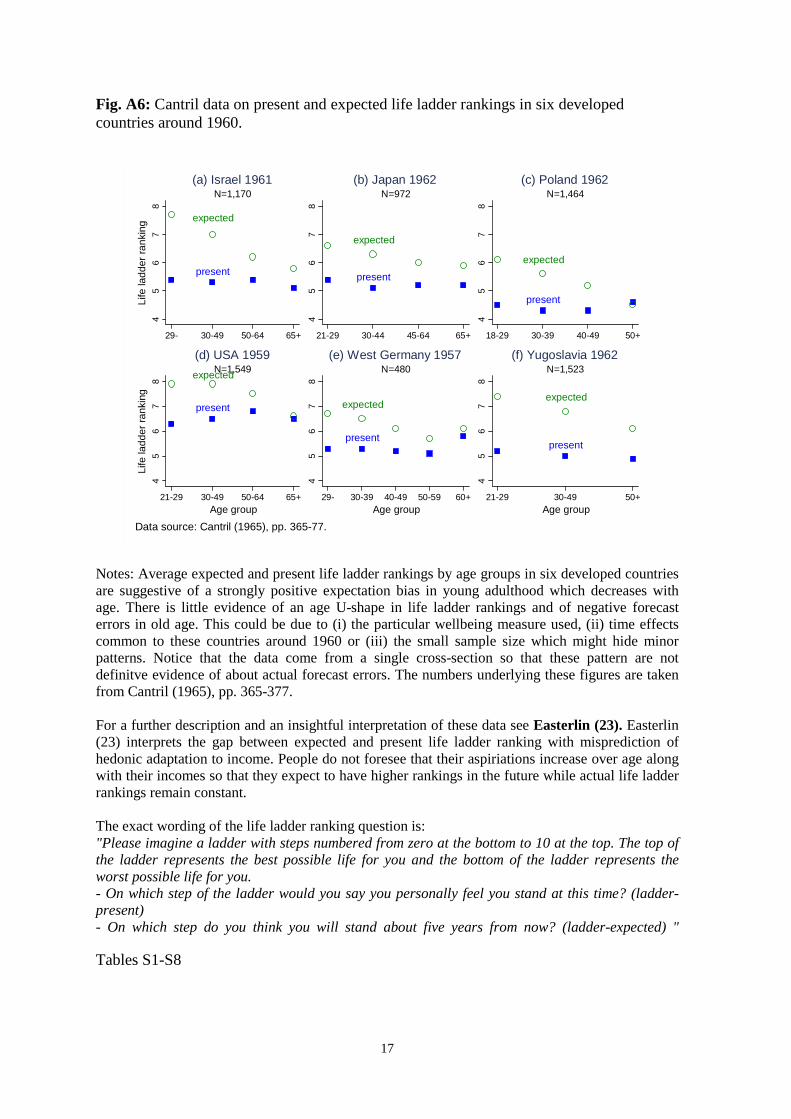
Fig. A6: Cantril data on present and expected life ladder rankings in six developed countries around 1960.

Notes: Average expected and present life ladder rankings by age groups in six developed countries are suggestive of a strongly positive expectation bias in young adulthood which decreases with age. There is little evidence of an age U-shape in life ladder rankings and of negative forecast errors in old age. This could be due to (i) the particular wellbeing measure used, (ii) time effects common to these countries around 1960 or (iii) the small sample size which might hide minor patterns. Notice that the data come from a single cross-section so that these pattern are not definitve evidence of about actual forecast errors. The numbers underlying these figures are taken from Cantril (1965), pp. 365-377. For a further description and an insightful interpretation of these data see Easterlin (23). Easterlin (23) interprets the gap between expected and present life ladder ranking with misprediction of hedonic adaptation to income. People do not foresee that their aspiriations increase over age along with their incomes so that they expect to have higher rankings in the future while actual life ladder rankings remain constant. The exact wording of the life ladder ranking question is: "Please imagine a ladder with steps numbered from zero at the bottom to 10 at the top. The top of the ladder represents the best possible life for you and the bottom of the ladder represents the worst possible life for you. - On which step of the ladder would you say you personally feel you stand at this time? (ladder-present) - On which step do you think you will stand about five years from now? (ladder-expected) " Tables S1-S8

present

expected

45

67

8

29- 30-49 50-64 65+

Life

ladd

er r

anki

ng

N=1,170 (a) Israel 1961

present

expected

45

67

8

21-29 30-44 45-64 65+

N=972 (b) Japan 1962

present

expected

45

67

8

18-29 30-39 40-49 50+

N=1,464 (c) Poland 1962

present

expected

45

67

8

21-29 30-49 50-64 65+

Life

ladd

er r

anki

ng

Age group

N=1,549 (d) USA 1959

present

expected

45

67

8

29- 30-39 40-49 50-59 60+ Age group

N=480 (e) West Germany 1957

present

expected

45

67

8

21-29 30-49 50+ Age group

N=1,523 (f) Yugoslavia 1962

Data source: Cantril (1965), pp. 365-77.

18

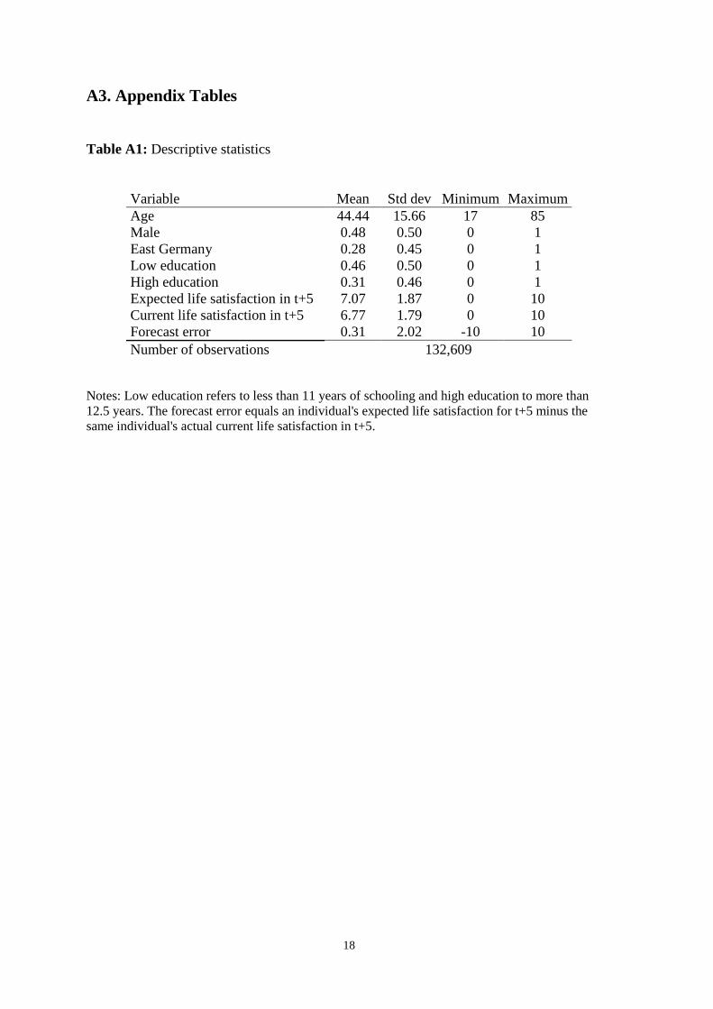
A3. Appendix Tables Table A1: Descriptive statistics

Variable Mean Std dev Minimum Maximum Age 44.44 15.66 17 85 Male 0.48 0.50 0 1 East Germany 0.28 0.45 0 1 Low education 0.46 0.50 0 1 High education 0.31 0.46 0 1 Expected life satisfaction in t+5 7.07 1.87 0 10 Current life satisfaction in t+5 6.77 1.79 0 10 Forecast error 0.31 2.02 -10 10 Number of observations 132,609

Notes: Low education refers to less than 11 years of schooling and high education to more than 12.5 years. The forecast error equals an individual's expected life satisfaction for t+5 minus the same individual's actual current life satisfaction in t+5.

19

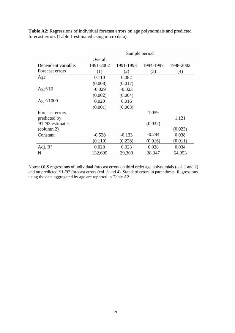
Table A2: Regressions of individual forecast errors on age polynomials and predicted forecast errors (Table 1 estimated using micro data).

Sample period Overall

Dependent variable: 1991-2002 1991-1993 1994-1997 1998-2002 Forecast errors (1) (2) (3) (4) Age 0.110 0.082

(0.008) (0.017) Age²/10 -0.029 -0.023

(0.002) (0.004) Age³/1000 0.020 0.016

(0.001) (0.003) Forecast errors predicted by

1.059 1.121

'91-'93 estimates (column 2)

(0.032) (0.023)

Constant -0.528 -0.133 -0.294 0.038 (0.110) (0.228) (0.016) (0.011) Adj. R² 0.028 0.023 0.028 0.034 N 132,609 29,309 38,347 64,953

Notes: OLS regressions of individual forecast errors on third order age polynomials (col. 1 and 2) and on predicted '91-'97 forecast errors (col. 3 and 4). Standard errors in parenthesis. Regressions using the data aggregated by age are reported in Table A2.

20

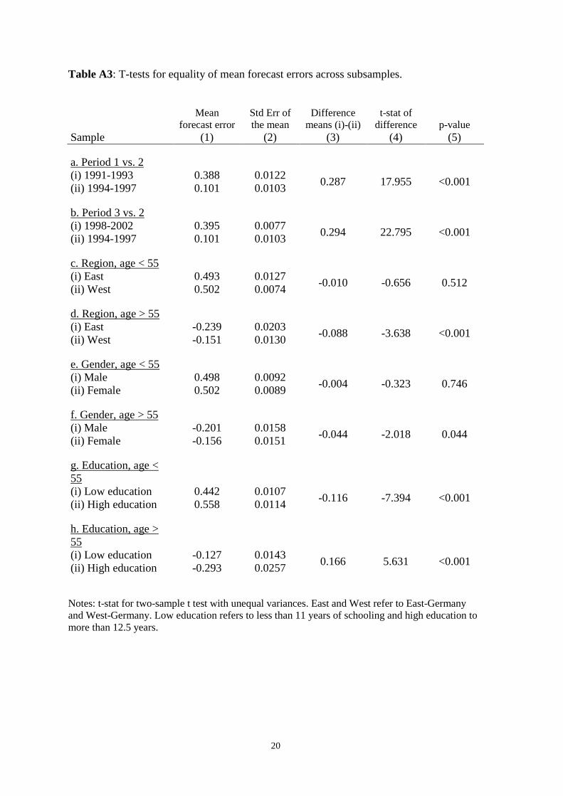
Table A3: T-tests for equality of mean forecast errors across subsamples.

Mean Std Err of Difference t-stat of forecast error the mean means (i)-(ii) difference p-value

Sample (1) (2) (3) (4) (5)

a. Period 1 vs. 2 (i) 1991-1993 0.388 0.0122

0.287 17.955 <0.001 (ii) 1994-1997 0.101 0.0103

b. Period 3 vs. 2 (i) 1998-2002 0.395 0.0077

0.294 22.795 <0.001 (ii) 1994-1997 0.101 0.0103

c. Region, age < 55 (i) East 0.493 0.0127

-0.010 -0.656 0.512 (ii) West 0.502 0.0074

d. Region, age > 55 (i) East -0.239 0.0203

-0.088 -3.638 <0.001 (ii) West -0.151 0.0130

e. Gender, age < 55 (i) Male 0.498 0.0092

-0.004 -0.323 0.746 (ii) Female 0.502 0.0089

f. Gender, age > 55 (i) Male -0.201 0.0158

-0.044 -2.018 0.044 (ii) Female -0.156 0.0151

g. Education, age < 55 (i) Low education 0.442 0.0107

-0.116 -7.394 <0.001 (ii) High education 0.558 0.0114

h. Education, age > 55 (i) Low education -0.127 0.0143

0.166 5.631 <0.001 (ii) High education -0.293 0.0257 Notes: t-stat for two-sample t test with unequal variances. East and West refer to East-Germany and West-Germany. Low education refers to less than 11 years of schooling and high education to more than 12.5 years.

21

Table A4: T-tests for equality of mean absolute forecast errors, low vs. high education

Mean absolute Std Err of Difference t-stat of forecast error the mean means (i)-(ii) difference p-value

Sample (1) (2) (3) (4) (4) A. Education, all ages (i) Low education 1.552 0.0059

0.226 23.527 <0.001 (ii) High education 1.326 0.0076

Notes: t-stat for two-sample t test with unequal variances. Low education refers to less than 11 years of schooling and high education to more than 12.5 years.

22

Table A5. Means of expected and current life satisfaction and forecast errors over age with standard errors (numerical values underlying Fig. 1)

Expected life Current life Forecast error satisfaction for t+5 satisfaction ( =Expected-Current[t+5] )

Mean SE(mean) Mean SE(mean) Mean SE(mean) Mean/Current[t+5] (1) (2) (3) (4) (5) (6) (7)

age=17 7.854 0.050 - - 0.792 0.065 0.112 age=18 7.777 0.045 - - 0.702 0.058 0.099 age=19 7.616 0.044 - - 0.608 0.055 0.087 age=20 7.677 0.041 - - 0.630 0.051 0.089 age=21 7.715 0.039 - - 0.685 0.047 0.098 age=22 7.711 0.037 7.062 0.054 0.638 0.047 0.090 age=23 7.745 0.034 7.075 0.045 0.693 0.044 0.098 age=24 7.684 0.034 7.008 0.043 0.625 0.041 0.089 age=25 7.709 0.033 7.047 0.041 0.684 0.040 0.097 age=26 7.679 0.032 7.029 0.039 0.680 0.039 0.097 age=27 7.685 0.031 7.073 0.037 0.711 0.038 0.102 age=28 7.676 0.030 7.052 0.035 0.728 0.036 0.105 age=29 7.623 0.031 7.059 0.035 0.665 0.037 0.096 age=30 7.604 0.029 7.025 0.034 0.673 0.035 0.097 age=31 7.552 0.029 7.000 0.033 0.620 0.034 0.089 age=32 7.511 0.030 6.974 0.032 0.640 0.034 0.093 age=33 7.440 0.031 6.948 0.031 0.589 0.034 0.086 age=34 7.406 0.030 6.957 0.031 0.577 0.033 0.085 age=35 7.368 0.031 6.930 0.032 0.579 0.035 0.085 age=36 7.338 0.030 6.932 0.030 0.587 0.034 0.087 age=37 7.259 0.031 6.871 0.031 0.542 0.034 0.081 age=38 7.196 0.032 6.851 0.031 0.530 0.034 0.080 age=39 7.200 0.032 6.829 0.031 0.524 0.035 0.079 age=40 7.072 0.033 6.789 0.031 0.437 0.036 0.066 age=41 7.088 0.033 6.750 0.031 0.486 0.036 0.074 age=42 7.046 0.034 6.717 0.031 0.479 0.038 0.073 age=43 6.996 0.035 6.666 0.032 0.436 0.037 0.066 age=44 6.927 0.036 6.676 0.033 0.411 0.039 0.063 age=45 6.880 0.037 6.634 0.033 0.352 0.039 0.054 age=46 6.865 0.038 6.601 0.034 0.328 0.040 0.050 age=47 6.800 0.039 6.567 0.035 0.301 0.041 0.046 age=48 6.804 0.039 6.560 0.035 0.307 0.041 0.047 age=49 6.760 0.040 6.516 0.036 0.216 0.042 0.033 age=50 6.750 0.040 6.528 0.037 0.233 0.043 0.036 age=51 6.782 0.040 6.537 0.038 0.153 0.042 0.023 age=52 6.704 0.040 6.499 0.039 0.090 0.040 0.014 age=53 6.709 0.040 6.498 0.038 0.107 0.041 0.016 age=54 6.686 0.041 6.544 0.038 0.082 0.043 0.012 age=55 6.648 0.041 6.517 0.038 -0.046 0.041 -0.007 age=56 6.658 0.041 6.629 0.037 -0.108 0.043 -0.016 age=57 6.658 0.040 6.614 0.038 -0.099 0.042 -0.015 age=58 6.659 0.041 6.602 0.038 -0.123 0.042 -0.018 age=59 6.598 0.042 6.604 0.038 -0.199 0.042 -0.029 age=60 6.597 0.042 6.694 0.037 -0.208 0.041 -0.031 age=61 6.614 0.042 6.767 0.037 -0.167 0.043 -0.025 age=62 6.631 0.043 6.757 0.036 -0.220 0.042 -0.032 age=63 6.679 0.045 6.781 0.037 -0.159 0.046 -0.023

23

age=64 6.610 0.046 6.797 0.037 -0.249 0.047 -0.036 age=65 6.591 0.049 6.805 0.037 -0.204 0.050 -0.030 age=66 6.617 0.049 6.781 0.038 -0.206 0.049 -0.030 age=67 6.589 0.051 6.850 0.038 -0.239 0.055 -0.035 age=68 6.508 0.053 6.837 0.042 -0.308 0.057 -0.045 age=69 6.619 0.057 6.860 0.042 -0.209 0.060 -0.031 age=70 6.575 0.059 6.795 0.045 -0.167 0.063 -0.025 age=71 6.572 0.061 6.823 0.045 -0.209 0.066 -0.031 age=72 6.574 0.063 6.827 0.049 -0.161 0.064 -0.024 age=73 6.617 0.069 6.816 0.052 -0.065 0.068 -0.010 age=74 6.580 0.070 6.828 0.055 -0.171 0.076 -0.025 age=75 6.572 0.077 6.742 0.058 -0.129 0.084 -0.019 age=76 6.484 0.081 6.781 0.060 -0.067 0.092 -0.010 age=77 6.394 0.087 6.736 0.061 -0.133 0.097 -0.020 age=78 6.420 0.098 6.682 0.066 -0.176 0.106 -0.027 age=79 6.521 0.103 6.751 0.070 -0.027 0.115 -0.004 age=80 6.467 0.118 6.702 0.076 -0.361 0.127 -0.053 age=81 6.340 0.126 6.550 0.082 -0.172 0.142 -0.026 age=82 6.389 0.146 6.527 0.090 -0.282 0.150 -0.042 age=83 6.315 0.172 6.597 0.095 -0.067 0.193 -0.011 age=84 6.169 0.189 6.548 0.106 -0.162 0.208 -0.026 age=85 6.177 0.186 6.828 0.106 -0.162 0.223 -0.025 age=86 - - 6.512 0.129 - - - age=87 - - 6.671 0.141 - - - age=88 - - 6.382 0.148 - - -

age=89 - - 6.331 0.180 - - -

age=90 - - 6.338 0.199 - - -

overall N 132,609 132,609 132,609

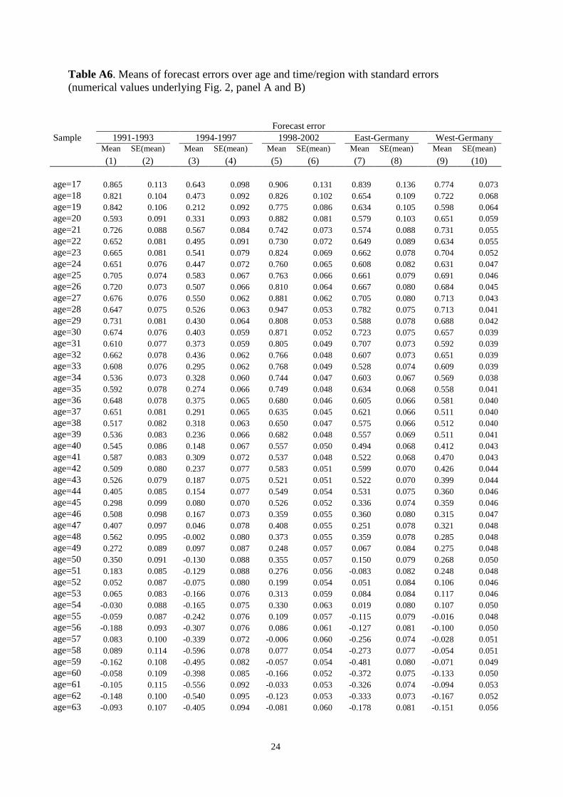
24

Table A6. Means of forecast errors over age and time/region with standard errors (numerical values underlying Fig. 2, panel A and B)

Forecast error Sample 1991-1993 1994-1997 1998-2002 East-Germany West-Germany

Mean SE(mean) Mean SE(mean) Mean SE(mean) Mean SE(mean) Mean SE(mean)

(1) (2) (3) (4) (5) (6) (7) (8) (9) (10) age=17 0.865 0.113 0.643 0.098 0.906 0.131 0.839 0.136 0.774 0.073 age=18 0.821 0.104 0.473 0.092 0.826 0.102 0.654 0.109 0.722 0.068 age=19 0.842 0.106 0.212 0.092 0.775 0.086 0.634 0.105 0.598 0.064 age=20 0.593 0.091 0.331 0.093 0.882 0.081 0.579 0.103 0.651 0.059 age=21 0.726 0.088 0.567 0.084 0.742 0.073 0.574 0.088 0.731 0.055 age=22 0.652 0.081 0.495 0.091 0.730 0.072 0.649 0.089 0.634 0.055 age=23 0.665 0.081 0.541 0.079 0.824 0.069 0.662 0.078 0.704 0.052 age=24 0.651 0.076 0.447 0.072 0.760 0.065 0.608 0.082 0.631 0.047 age=25 0.705 0.074 0.583 0.067 0.763 0.066 0.661 0.079 0.691 0.046 age=26 0.720 0.073 0.507 0.066 0.810 0.064 0.667 0.080 0.684 0.045 age=27 0.676 0.076 0.550 0.062 0.881 0.062 0.705 0.080 0.713 0.043 age=28 0.647 0.075 0.526 0.063 0.947 0.053 0.782 0.075 0.713 0.041 age=29 0.731 0.081 0.430 0.064 0.808 0.053 0.588 0.078 0.688 0.042 age=30 0.674 0.076 0.403 0.059 0.871 0.052 0.723 0.075 0.657 0.039 age=31 0.610 0.077 0.373 0.059 0.805 0.049 0.707 0.073 0.592 0.039 age=32 0.662 0.078 0.436 0.062 0.766 0.048 0.607 0.073 0.651 0.039 age=33 0.608 0.076 0.295 0.062 0.768 0.049 0.528 0.074 0.609 0.039 age=34 0.536 0.073 0.328 0.060 0.744 0.047 0.603 0.067 0.569 0.038 age=35 0.592 0.078 0.274 0.066 0.749 0.048 0.634 0.068 0.558 0.041 age=36 0.648 0.078 0.375 0.065 0.680 0.046 0.605 0.066 0.581 0.040 age=37 0.651 0.081 0.291 0.065 0.635 0.045 0.621 0.066 0.511 0.040 age=38 0.517 0.082 0.318 0.063 0.650 0.047 0.575 0.066 0.512 0.040 age=39 0.536 0.083 0.236 0.066 0.682 0.048 0.557 0.069 0.511 0.041 age=40 0.545 0.086 0.148 0.067 0.557 0.050 0.494 0.068 0.412 0.043 age=41 0.587 0.083 0.309 0.072 0.537 0.048 0.522 0.068 0.470 0.043 age=42 0.509 0.080 0.237 0.077 0.583 0.051 0.599 0.070 0.426 0.044 age=43 0.526 0.079 0.187 0.075 0.521 0.051 0.522 0.070 0.399 0.044 age=44 0.405 0.085 0.154 0.077 0.549 0.054 0.531 0.075 0.360 0.046 age=45 0.298 0.099 0.080 0.070 0.526 0.052 0.336 0.074 0.359 0.046 age=46 0.508 0.098 0.167 0.073 0.359 0.055 0.360 0.080 0.315 0.047 age=47 0.407 0.097 0.046 0.078 0.408 0.055 0.251 0.078 0.321 0.048 age=48 0.562 0.095 -0.002 0.080 0.373 0.055 0.359 0.078 0.285 0.048 age=49 0.272 0.089 0.097 0.087 0.248 0.057 0.067 0.084 0.275 0.048 age=50 0.350 0.091 -0.130 0.088 0.355 0.057 0.150 0.079 0.268 0.050 age=51 0.183 0.085 -0.129 0.088 0.276 0.056 -0.083 0.082 0.248 0.048 age=52 0.052 0.087 -0.075 0.080 0.199 0.054 0.051 0.084 0.106 0.046 age=53 0.065 0.083 -0.166 0.076 0.313 0.059 0.084 0.084 0.117 0.046 age=54 -0.030 0.088 -0.165 0.075 0.330 0.063 0.019 0.080 0.107 0.050 age=55 -0.059 0.087 -0.242 0.076 0.109 0.057 -0.115 0.079 -0.016 0.048 age=56 -0.188 0.093 -0.307 0.076 0.086 0.061 -0.127 0.081 -0.100 0.050 age=57 0.083 0.100 -0.339 0.072 -0.006 0.060 -0.256 0.074 -0.028 0.051 age=58 0.089 0.114 -0.596 0.078 0.077 0.054 -0.273 0.077 -0.054 0.051 age=59 -0.162 0.108 -0.495 0.082 -0.057 0.054 -0.481 0.080 -0.071 0.049 age=60 -0.058 0.109 -0.398 0.085 -0.166 0.052 -0.372 0.075 -0.133 0.050 age=61 -0.105 0.115 -0.556 0.092 -0.033 0.053 -0.326 0.074 -0.094 0.053 age=62 -0.148 0.100 -0.540 0.095 -0.123 0.053 -0.333 0.073 -0.167 0.052 age=63 -0.093 0.107 -0.405 0.094 -0.081 0.060 -0.178 0.081 -0.151 0.056

25

age=64 -0.377 0.111 -0.468 0.092 -0.119 0.061 -0.332 0.084 -0.212 0.056 age=65 -0.066 0.117 -0.437 0.095 -0.138 0.068 -0.310 0.091 -0.158 0.060 age=66 0.064 0.113 -0.432 0.099 -0.183 0.064 -0.288 0.092 -0.171 0.057 age=67 -0.223 0.138 -0.405 0.102 -0.162 0.073 -0.220 0.105 -0.246 0.064 age=68 -0.119 0.139 -0.452 0.109 -0.307 0.075 -0.367 0.106 -0.284 0.067 age=69 -0.051 0.149 -0.498 0.110 -0.129 0.080 -0.187 0.125 -0.217 0.068 age=70 0.013 0.147 -0.446 0.122 -0.104 0.084 -0.126 0.120 -0.181 0.074 age=71 -0.156 0.156 -0.299 0.123 -0.188 0.089 0.082 0.128 -0.307 0.076 age=72 -0.158 0.174 -0.317 0.127 -0.086 0.080 -0.129 0.132 -0.172 0.073 age=73 -0.092 0.208 -0.156 0.129 -0.012 0.085 -0.133 0.128 -0.042 0.080 age=74 -0.211 0.259 -0.187 0.145 -0.155 0.093 -0.095 0.140 -0.196 0.090 age=75 0.038 0.236 -0.205 0.173 -0.126 0.105 0.065 0.169 -0.190 0.097 age=76 -0.135 0.248 0.020 0.198 -0.085 0.113 0.089 0.189 -0.110 0.105 age=77 -0.322 0.301 -0.071 0.213 -0.105 0.114 0.008 0.162 -0.176 0.117 age=78 -0.506 0.242 -0.060 0.277 -0.122 0.128 0.170 0.213 -0.280 0.121 age=79 -0.083 0.250 -0.284 0.276 0.061 0.145 -0.084 0.256 -0.010 0.128 age=80 -0.088 0.277 -0.797 0.284 -0.303 0.165 -0.036 0.252 -0.469 0.147 age=81 0.000 0.305 -0.818 0.304 0.018 0.186 0.139 0.287 -0.271 0.163 age=82 0.036 0.257 -0.971 0.290 -0.018 0.224 0.034 0.266 -0.386 0.179 age=83 -0.250 0.437 0.052 0.329 -0.063 0.286 0.171 0.483 -0.139 0.206 age=84 -0.143 0.597 -0.176 0.347 -0.160 0.282 -0.441 0.412 -0.083 0.240 age=85 -0.278 0.718 -0.195 0.344 -0.113 0.312 -0.875 0.460 0.000 0.252 overall N 29,309 38,347 64,953 37,070 95,539

26

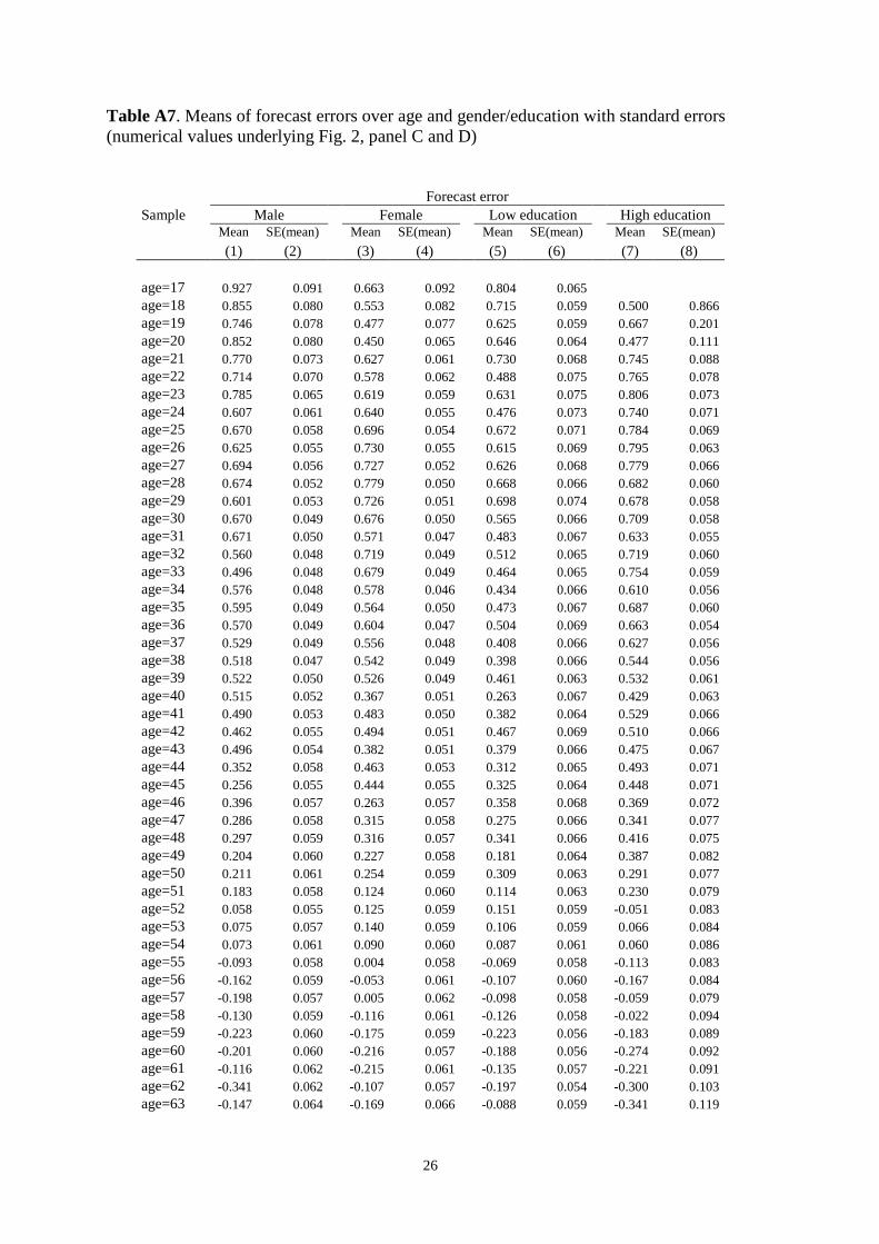
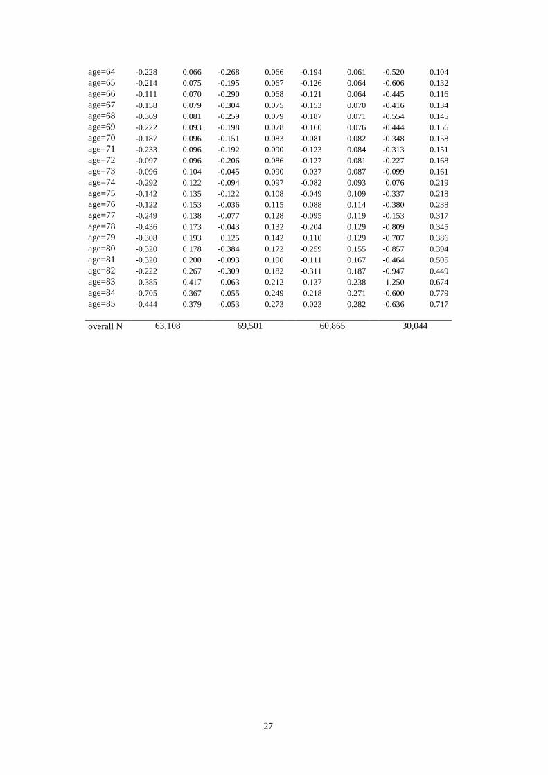
Table A7. Means of forecast errors over age and gender/education with standard errors (numerical values underlying Fig. 2, panel C and D)

Forecast error Sample Male Female Low education High education

Mean SE(mean) Mean SE(mean) Mean SE(mean) Mean SE(mean)

(1) (2) (3) (4) (5) (6) (7) (8) age=17 0.927 0.091 0.663 0.092 0.804 0.065 age=18 0.855 0.080 0.553 0.082 0.715 0.059 0.500 0.866 age=19 0.746 0.078 0.477 0.077 0.625 0.059 0.667 0.201 age=20 0.852 0.080 0.450 0.065 0.646 0.064 0.477 0.111 age=21 0.770 0.073 0.627 0.061 0.730 0.068 0.745 0.088 age=22 0.714 0.070 0.578 0.062 0.488 0.075 0.765 0.078 age=23 0.785 0.065 0.619 0.059 0.631 0.075 0.806 0.073 age=24 0.607 0.061 0.640 0.055 0.476 0.073 0.740 0.071 age=25 0.670 0.058 0.696 0.054 0.672 0.071 0.784 0.069 age=26 0.625 0.055 0.730 0.055 0.615 0.069 0.795 0.063 age=27 0.694 0.056 0.727 0.052 0.626 0.068 0.779 0.066 age=28 0.674 0.052 0.779 0.050 0.668 0.066 0.682 0.060 age=29 0.601 0.053 0.726 0.051 0.698 0.074 0.678 0.058 age=30 0.670 0.049 0.676 0.050 0.565 0.066 0.709 0.058 age=31 0.671 0.050 0.571 0.047 0.483 0.067 0.633 0.055 age=32 0.560 0.048 0.719 0.049 0.512 0.065 0.719 0.060 age=33 0.496 0.048 0.679 0.049 0.464 0.065 0.754 0.059 age=34 0.576 0.048 0.578 0.046 0.434 0.066 0.610 0.056 age=35 0.595 0.049 0.564 0.050 0.473 0.067 0.687 0.060 age=36 0.570 0.049 0.604 0.047 0.504 0.069 0.663 0.054 age=37 0.529 0.049 0.556 0.048 0.408 0.066 0.627 0.056 age=38 0.518 0.047 0.542 0.049 0.398 0.066 0.544 0.056 age=39 0.522 0.050 0.526 0.049 0.461 0.063 0.532 0.061 age=40 0.515 0.052 0.367 0.051 0.263 0.067 0.429 0.063 age=41 0.490 0.053 0.483 0.050 0.382 0.064 0.529 0.066 age=42 0.462 0.055 0.494 0.051 0.467 0.069 0.510 0.066 age=43 0.496 0.054 0.382 0.051 0.379 0.066 0.475 0.067 age=44 0.352 0.058 0.463 0.053 0.312 0.065 0.493 0.071 age=45 0.256 0.055 0.444 0.055 0.325 0.064 0.448 0.071 age=46 0.396 0.057 0.263 0.057 0.358 0.068 0.369 0.072 age=47 0.286 0.058 0.315 0.058 0.275 0.066 0.341 0.077 age=48 0.297 0.059 0.316 0.057 0.341 0.066 0.416 0.075 age=49 0.204 0.060 0.227 0.058 0.181 0.064 0.387 0.082 age=50 0.211 0.061 0.254 0.059 0.309 0.063 0.291 0.077 age=51 0.183 0.058 0.124 0.060 0.114 0.063 0.230 0.079 age=52 0.058 0.055 0.125 0.059 0.151 0.059 -0.051 0.083 age=53 0.075 0.057 0.140 0.059 0.106 0.059 0.066 0.084 age=54 0.073 0.061 0.090 0.060 0.087 0.061 0.060 0.086 age=55 -0.093 0.058 0.004 0.058 -0.069 0.058 -0.113 0.083 age=56 -0.162 0.059 -0.053 0.061 -0.107 0.060 -0.167 0.084 age=57 -0.198 0.057 0.005 0.062 -0.098 0.058 -0.059 0.079 age=58 -0.130 0.059 -0.116 0.061 -0.126 0.058 -0.022 0.094 age=59 -0.223 0.060 -0.175 0.059 -0.223 0.056 -0.183 0.089 age=60 -0.201 0.060 -0.216 0.057 -0.188 0.056 -0.274 0.092 age=61 -0.116 0.062 -0.215 0.061 -0.135 0.057 -0.221 0.091 age=62 -0.341 0.062 -0.107 0.057 -0.197 0.054 -0.300 0.103 age=63 -0.147 0.064 -0.169 0.066 -0.088 0.059 -0.341 0.119

27

age=64 -0.228 0.066 -0.268 0.066 -0.194 0.061 -0.520 0.104 age=65 -0.214 0.075 -0.195 0.067 -0.126 0.064 -0.606 0.132 age=66 -0.111 0.070 -0.290 0.068 -0.121 0.064 -0.445 0.116 age=67 -0.158 0.079 -0.304 0.075 -0.153 0.070 -0.416 0.134 age=68 -0.369 0.081 -0.259 0.079 -0.187 0.071 -0.554 0.145 age=69 -0.222 0.093 -0.198 0.078 -0.160 0.076 -0.444 0.156 age=70 -0.187 0.096 -0.151 0.083 -0.081 0.082 -0.348 0.158 age=71 -0.233 0.096 -0.192 0.090 -0.123 0.084 -0.313 0.151 age=72 -0.097 0.096 -0.206 0.086 -0.127 0.081 -0.227 0.168 age=73 -0.096 0.104 -0.045 0.090 0.037 0.087 -0.099 0.161 age=74 -0.292 0.122 -0.094 0.097 -0.082 0.093 0.076 0.219 age=75 -0.142 0.135 -0.122 0.108 -0.049 0.109 -0.337 0.218 age=76 -0.122 0.153 -0.036 0.115 0.088 0.114 -0.380 0.238 age=77 -0.249 0.138 -0.077 0.128 -0.095 0.119 -0.153 0.317 age=78 -0.436 0.173 -0.043 0.132 -0.204 0.129 -0.809 0.345 age=79 -0.308 0.193 0.125 0.142 0.110 0.129 -0.707 0.386 age=80 -0.320 0.178 -0.384 0.172 -0.259 0.155 -0.857 0.394 age=81 -0.320 0.200 -0.093 0.190 -0.111 0.167 -0.464 0.505 age=82 -0.222 0.267 -0.309 0.182 -0.311 0.187 -0.947 0.449 age=83 -0.385 0.417 0.063 0.212 0.137 0.238 -1.250 0.674 age=84 -0.705 0.367 0.055 0.249 0.218 0.271 -0.600 0.779 age=85 -0.444 0.379 -0.053 0.273 0.023 0.282 -0.636 0.717 overall N 63,108 69,501 60,865 30,044

28

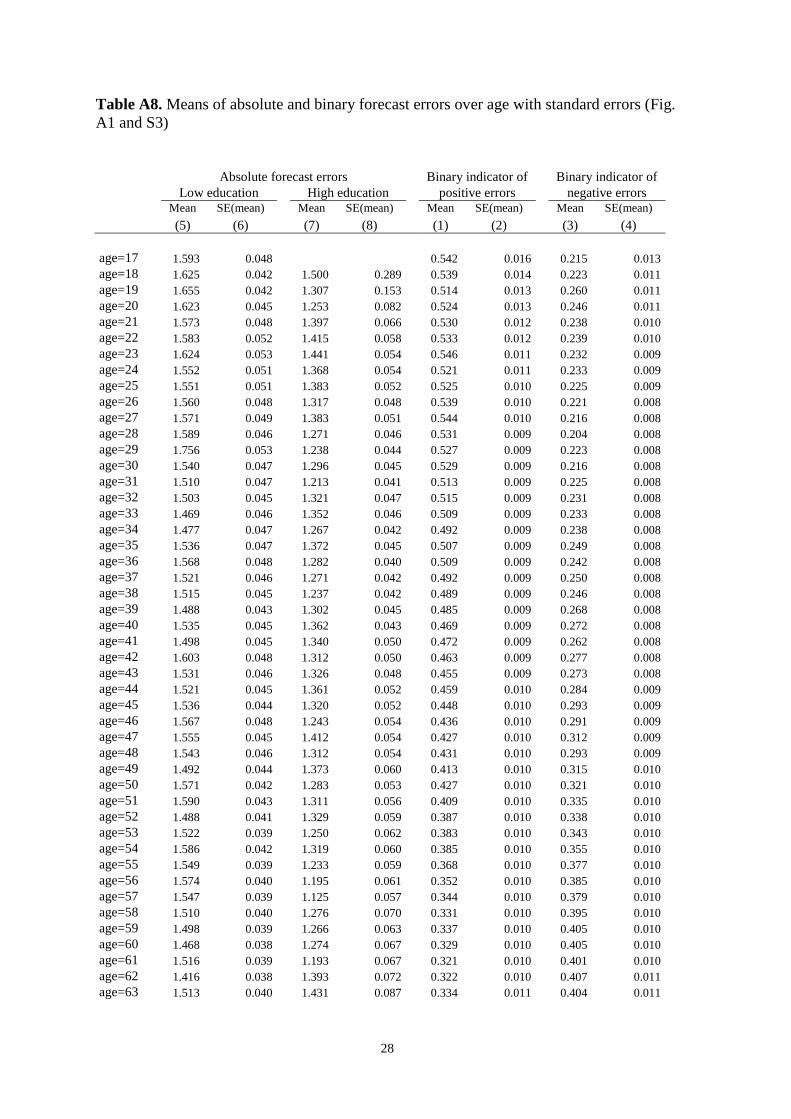
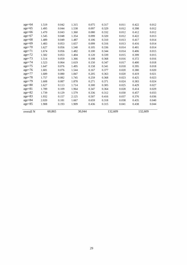
Table A8. Means of absolute and binary forecast errors over age with standard errors (Fig. A1 and S3)

Absolute forecast errors Binary indicator of Binary indicator of Low education High education positive errors negative errors

Mean SE(mean) Mean SE(mean) Mean SE(mean) Mean SE(mean)

(5) (6) (7) (8) (1) (2) (3) (4) age=17 1.593 0.048 0.542 0.016 0.215 0.013 age=18 1.625 0.042 1.500 0.289 0.539 0.014 0.223 0.011 age=19 1.655 0.042 1.307 0.153 0.514 0.013 0.260 0.011 age=20 1.623 0.045 1.253 0.082 0.524 0.013 0.246 0.011 age=21 1.573 0.048 1.397 0.066 0.530 0.012 0.238 0.010 age=22 1.583 0.052 1.415 0.058 0.533 0.012 0.239 0.010 age=23 1.624 0.053 1.441 0.054 0.546 0.011 0.232 0.009 age=24 1.552 0.051 1.368 0.054 0.521 0.011 0.233 0.009 age=25 1.551 0.051 1.383 0.052 0.525 0.010 0.225 0.009 age=26 1.560 0.048 1.317 0.048 0.539 0.010 0.221 0.008 age=27 1.571 0.049 1.383 0.051 0.544 0.010 0.216 0.008 age=28 1.589 0.046 1.271 0.046 0.531 0.009 0.204 0.008 age=29 1.756 0.053 1.238 0.044 0.527 0.009 0.223 0.008 age=30 1.540 0.047 1.296 0.045 0.529 0.009 0.216 0.008 age=31 1.510 0.047 1.213 0.041 0.513 0.009 0.225 0.008 age=32 1.503 0.045 1.321 0.047 0.515 0.009 0.231 0.008 age=33 1.469 0.046 1.352 0.046 0.509 0.009 0.233 0.008 age=34 1.477 0.047 1.267 0.042 0.492 0.009 0.238 0.008 age=35 1.536 0.047 1.372 0.045 0.507 0.009 0.249 0.008 age=36 1.568 0.048 1.282 0.040 0.509 0.009 0.242 0.008 age=37 1.521 0.046 1.271 0.042 0.492 0.009 0.250 0.008 age=38 1.515 0.045 1.237 0.042 0.489 0.009 0.246 0.008 age=39 1.488 0.043 1.302 0.045 0.485 0.009 0.268 0.008 age=40 1.535 0.045 1.362 0.043 0.469 0.009 0.272 0.008 age=41 1.498 0.045 1.340 0.050 0.472 0.009 0.262 0.008 age=42 1.603 0.048 1.312 0.050 0.463 0.009 0.277 0.008 age=43 1.531 0.046 1.326 0.048 0.455 0.009 0.273 0.008 age=44 1.521 0.045 1.361 0.052 0.459 0.010 0.284 0.009 age=45 1.536 0.044 1.320 0.052 0.448 0.010 0.293 0.009 age=46 1.567 0.048 1.243 0.054 0.436 0.010 0.291 0.009 age=47 1.555 0.045 1.412 0.054 0.427 0.010 0.312 0.009 age=48 1.543 0.046 1.312 0.054 0.431 0.010 0.293 0.009 age=49 1.492 0.044 1.373 0.060 0.413 0.010 0.315 0.010 age=50 1.571 0.042 1.283 0.053 0.427 0.010 0.321 0.010 age=51 1.590 0.043 1.311 0.056 0.409 0.010 0.335 0.010 age=52 1.488 0.041 1.329 0.059 0.387 0.010 0.338 0.010 age=53 1.522 0.039 1.250 0.062 0.383 0.010 0.343 0.010 age=54 1.586 0.042 1.319 0.060 0.385 0.010 0.355 0.010 age=55 1.549 0.039 1.233 0.059 0.368 0.010 0.377 0.010 age=56 1.574 0.040 1.195 0.061 0.352 0.010 0.385 0.010 age=57 1.547 0.039 1.125 0.057 0.344 0.010 0.379 0.010 age=58 1.510 0.040 1.276 0.070 0.331 0.010 0.395 0.010 age=59 1.498 0.039 1.266 0.063 0.337 0.010 0.405 0.010 age=60 1.468 0.038 1.274 0.067 0.329 0.010 0.405 0.010 age=61 1.516 0.039 1.193 0.067 0.321 0.010 0.401 0.010 age=62 1.416 0.038 1.393 0.072 0.322 0.010 0.407 0.011 age=63 1.513 0.040 1.431 0.087 0.334 0.011 0.404 0.011

29

age=64 1.519 0.042 1.315 0.075 0.317 0.011 0.422 0.012 age=65 1.495 0.044 1.538 0.097 0.329 0.012 0.398 0.012 age=66 1.470 0.043 1.360 0.080 0.332 0.012 0.412 0.012 age=67 1.545 0.048 1.354 0.099 0.320 0.012 0.422 0.013 age=68 1.489 0.049 1.487 0.106 0.310 0.013 0.417 0.014 age=69 1.483 0.053 1.657 0.099 0.316 0.013 0.416 0.014 age=70 1.627 0.056 1.540 0.105 0.336 0.014 0.401 0.014 age=71 1.674 0.056 1.482 0.100 0.344 0.014 0.406 0.015 age=72 1.582 0.053 1.404 0.120 0.339 0.015 0.399 0.015 age=73 1.514 0.059 1.366 0.108 0.368 0.016 0.372 0.016 age=74 1.523 0.064 1.619 0.150 0.347 0.017 0.400 0.018 age=75 1.647 0.076 1.495 0.158 0.341 0.018 0.395 0.018 age=76 1.681 0.076 1.544 0.167 0.377 0.020 0.380 0.020 age=77 1.689 0.080 1.847 0.205 0.363 0.020 0.419 0.021 age=78 1.757 0.082 1.745 0.259 0.368 0.023 0.425 0.023 age=79 1.608 0.087 1.878 0.271 0.371 0.024 0.383 0.024 age=80 1.627 0.113 1.714 0.300 0.305 0.025 0.429 0.027 age=81 1.789 0.109 1.964 0.347 0.364 0.028 0.414 0.029 age=82 1.739 0.129 1.579 0.336 0.312 0.030 0.457 0.033 age=83 1.932 0.157 2.125 0.507 0.416 0.037 0.376 0.036 age=84 2.020 0.181 1.667 0.659 0.318 0.038 0.435 0.040 age=85 1.908 0.193 1.909 0.436 0.315 0.041 0.438 0.044 overall N 60,865 30,044 132,609 132,609

30

6. References

1. Oswald AJ, Wu S (2010) Objective confirmation of subjective measures of human well-being: Evidence from the U.S.A.. Science 327:576-579

2. Easterlin RA (2003) Explaining happiness. Proceedings of the National Academy of Sciences U.S.A. 100:11176-11183

3. Clark AE, Frijters P, Shield MA (2008) Relative income, happiness, and utility: An explanation for the Easterlin paradox and other puzzles. Journal of Economic Literature 46:95-144

4. Blanchflower DG, Oswald AJ (2008) Is well-being U-shaped over the life cycle? Social Science & Medicine 66:1733-1749

5. Stone AA, Schwartz JE, Broderick JE, Deaton A (2010) A snapshot of the age distribution of psychological well-being in the United States. Proceedings of the National Academy of Sciences U.S.A. 107:9985-9990 (2010)

6. Van Landeghem B (2012) A test for the convexity of human well-being over the life cycle: Longitudinal evidence from a 20-year panel. Journal of Economic Behavior & Organization 81:571-582

7. Weiss A, King KE, Inoue-Murayama M, Matsuzawa T, Oswald AJ (2012) Evidence for a midlife crisis in great apes consistent with the U-shape in human well-being. Proceedings of the National Academy of Sciences U.S.A. 109, 19949-19952:2012

8. Frey BS, Stutzer A (2002) Happiness and Economics (Princeton Univ. Press, Princeton)

9. Frijters P, Beatton T (2012) The mystery of the U-shaped relationship between happiness and age. Journal of Economic Behavior & Organization 82:525–542.

10. Brassen S, Gamer M, Peters J, Gluth S, Büchel C (2012) Don't look back in anger! Responsiveness to missed chances in successful and nonsuccessful aging. Science 336:612-614

11. Weinstein ND (1980) Unrealistic optimism about future life events. Journal of Personality and Social Psychology 39:806-820

12. Puri M, Robinson DT (2007) Optimism and economic choice. Journal of Financial Economics 86:71-99

13. Sharot T, Riccardi AM, Raio CM, Phelps EA (2007) Neural mechanisms mediating optimism bias. Nature 450:102-105

31

14. Sharot T, Korn CW, Dolan RJ (2011) How unrealistic optimism is maintained in the face of reality. Nature Neuroscience 14:1475-1479

15. Sharot T, Kanai R, Marston D, Korn CW, Rees G, Dolan RJ (2012) Selectively altering belief formation in the human brain. Proceedings of the National Academy of Sciences U.S.A. 109:17058-17062

16. Loewenstein GF, Schkade D (1999) in Well-Being: The Foundations of Hedonic Psychology, Diener E, Schwartz N, Kahneman D (eds), Russell Sage Foundation: New York.

17. Kahneman D, Thaler R (2006) Anomalies: Utility maximization and experienced utility. Journal of Economic Perspectives 20:221-234

18. Kahneman D, Deaton A (2010) High income improves evaluation of life but not emotional well-being. Proceedings of the National Academy of Sciences U.S.A. 107:16489-16493

19. Benjamin DJ, Heffetz O, Kimball MS, Rees-Jones A (2012) What Do You Think Would Make You Happier? What Do You Think You Would Choose? American Economic Review 102:2083-2110

20. Ferrer-i-Carbonell A, Frijters P (2004) How important is methodology for the estimates of the determinants of happiness? Economic Journal 114:641-659

21. Alesina A, Fuchs-Schündeln N (2007) Good bye Lenin (or not?): The effect of Communism on people's preferences. American Economic Review 97:1507-1528

22. Easterlin RA (2001) Income and happiness: Towards a unified theory. Economic Journal 111:465-484

23. Cantril H (1965) The pattern of human concerns. (New Brunswick, NJ, Rutgers Univ. Press)

24. Mayraz, G (2011) Wishful Thinking. Discussion Paper No. 1092, Centre for Economic Performance, London School of Economics

25. Matheson SM, Asher L, Bateson M, (2008) Larger, enriched cages are associated with ‘optimistic’ response biases in captive European starlings (Sturnus vulgaris). Applied Animal Behaviour Science 109:374-383

26. Isaacowitz DM (2005) Correlates of well-being in adulthood and old age: A tale of two optimisms, Journal of Research in Personality 39:224-244

32

27. Wagner G, Frick J, Schupp J (2007) The German Socio-Economic Panel study (SOEP)-evolution, scope and enhancements. Schmollers Jahrbuch 127:139-169

28. Kahneman D, Krueger AB, Schkade D, Schwarz N, Stone AA (2006) Would You Be Happier If You Were Richer? A Focusing Illusion, Science 312:1908-1910

CENTRE FOR ECONOMIC PERFORMANCE

Recent Discussion Papers

1228 Bénédicte Apouey

Andrew E. Clark

Winning Big But Feeling No Better? The

Effect of Lottery Prizes on Physical and

Mental Health

1227 Alex Gyani

Roz Shafran

Richard Layard

David M Clark

Enhancing Recovery Rates:

Lessons from Year One of the English

Improving Access to Psychological

Therapies Programme

1226 Stephen Gibbons

Sandra McNally

The Effects of Resources Across School

Phases: A Summary of Recent Evidence

1225 Cornelius A. Rietveld

David Cesarini

Daniel J. Benjamin

Philipp D. Koellinger

Jan-Emmanuel De Neve

Henning Tiemeier

Magnus Johannesson

Patrik K.E. Magnusson

Nancy L. Pedersen

Robert F. Krueger

Meike Bartels

Molecular Genetics and Subjective Well-

Being

1224 Peter Arcidiacono

Esteban Aucejo

Patrick Coate

V. Joseph Hotz

Affirmative Action and University Fit:

Evidence from Proposition 209

1223 Peter Arcidiacono

Esteban Aucejo

V. Joseph Hotz

University Differences in the Graduation of

Minorities in STEM Fields: Evidence from

California

1222 Paul Dolan

Robert Metcalfe

Neighbors, Knowledge, and Nuggets: Two

Natural Field Experiments on the Role of

Incentives on Energy Conservation

1221 Andy Feng

Georg Graetz

A Question of Degree: The Effects of Degree

Class on Labor Market Outcomes

1220 Esteban Aucejo Explaining Cross-Racial Differences in the

Educational Gender Gap

1219 Peter Arcidiacono

Esteban Aucejo

Andrew Hussey

Kenneth Spenner

Racial Segregation Patterns in Selective

Universities

1218 Silvana Tenreyro

Gregory Thwaites

Pushing On a String: US Monetary Policy is

Less Powerful in Recessions

1217 Gianluca Benigno

Luca Fornaro

The Financial Resource Curse

1216 Daron Acemoglu

Ufuk Akcigit

Nicholas Bloom

William R. Kerr

Innovation, Reallocation and Growth

1215 Michael J. Boehm Has Job Polarization Squeezed the Middle

Class? Evidence from the Allocation of

Talents

1214 Nattavudh Powdthavee

Warn N. Lekfuangfu

Mark Wooden

The Marginal Income Effect of Education on

Happiness: Estimating the Direct and Indirect

Effects of Compulsory Schooling on Well-

Being in Australia

1213 Richard Layard Mental Health: The New Frontier for Labour

Economics

1212 Francesco Caselli

Massimo Morelli

Dominic Rohner

The Geography of Inter-State Resource Wars

1211 Stephen Hansen

Michael McMahon

Estimating Bayesian Decision Problems with

Heterogeneous Priors

1210 Christopher A. Pissarides Unemployment in the Great Recession

1209 Kevin D. Sheedy Debt and Incomplete Financial Markets: A

Case for Nominal GDP Targeting

1208 Jordi Blanes i Vidal

Marc Möller

Decision-Making and Implementation in

Teams

1207 Michael J. Boehm Concentration versus Re-Matching? Evidence

About the Locational Effects of Commuting

Costs

1206 Antonella Nocco

Gianmarco I. P. Ottaviano

Matteo Salto

Monopolistic Competition and Optimum

Product Selection: Why and How

Heterogeneity Matters

1205 Alberto Galasso

Mark Schankerman

Patents and Cumulative Innovation: Causal

Evidence from the Courts

1204 L Rachel Ngai

Barbara Petrongolo

Gender Gaps and the Rise of the Service

Economy

The Centre for Economic Performance Publications Unit

Tel 020 7955 7673 Fax 020 7404 0612

Email info@cep.lse.ac.uk Web site http://cep.lse.ac.uk