Embed Size (px)
Citation preview

Centre for Marine Science and Technology Curtin University
REPORT ON A TWO YEAR UNDERWATER NOISE
MEASUREMENT PROGRAM: BEFORE, DURING AND AFTER DREDGING AND PORT CONSTRUCTION
ACTIVITY IN DARWIN HARBOUR, 2012-2015 FINAL REPORT
By:
Salgado-Kent, C.1, Pusey, G.2, Gavrilov, A.1, Parsons, M.1, McCauley, R. 1
1, Riddoch, N.1, Parnum, I.1, Marley, S.1, and Lucke, K.1
1Centre for Marine Science and Technology (CMST), Curtin University, GPO Box U 1987 Perth 6845, WA
2RPS, 31 Bishop Street, Jolimont 6014, Western Australia
November 2015
For – CARDNO
PROJECT CMST 1122 REPORT 2015-10

Underwater Noise Monitoring Final Report Ichthys Nearshore Environmental Monitoring Program
Prepared for Cardno Curtin University ii
Executive Summary The Underwater Noise Monitoring Program was developed to monitor underwater noise levels within the vicinity of construction activities (dredging and piling) in Darwin Harbour associated with the Ichthys LNG Project (the Project). The program objectives were to verify underwater noise levels modelled in the EIS, and to conduct long-term underwater noise monitoring prior to, during and following the completion of construction activities and where required to inform potential changes in abundance and distribution of marine fauna. To verify the underwater noise models, in situ and acoustic logger measurements of underwater noise emitted from dredging and pile driving operations were collected. Verification of dredging noise levels are reported here. Verification of pile driving noise levels are reported in a separate monitoring program (INPEX 2014b).
The objective of the long-term monitoring program was to describe the dominant sources of underwater noise in the soundscape of Middle Arm and East Arm including biological, physical and anthropogenic with main emphasis on dredging, machinery and vessel noise. Long-term underwater noise monitoring was conducted using stationary autonomous sea noise recorders (noise loggers) deployed for 26 months from November 2012 to January 2015. The noise loggers deployed at Middle Arm measured the soundscape away from construction activity, and loggers deployed at East Arm measured the soundscape within the vicinity of construction activities.
The noise measurements made during the program confirmed that the underwater noise profile within Darwin Harbour is noisy from biological, physical and anthropogenic sources.
The underwater noise environment in East Arm was dominated by noises of man-made origin. The most intense noise recorded was from marine piling, followed by dredging. Dredging and/or pile driving was undertaken intermittently during 23 months: 6 months of dredging only, 9 months of piling only, and 8 months of which both dredging and pile driving were present. Dredging noise was recorded sometimes over periods lasting from about 1 to 5 hours, with short breaks in noise before it resumed. This noise was most intense between mid-December 2012 and mid-April 2013, when loggers were located closest to dredge operations. The noise was broadband, ranging from approximately 20 Hz to nearly 5 kHz with intensity levels reaching close to 160 dB re 1 Pa during some periods.
Received noise levels produced during dredging at Walker Shoal were a focus due to the hard substratum being dredged. The analyses revealed noise levels close to approximately 145 dB re 1 µPa at distances between 630 m and 680 m from the source. These levels were greater than the predicted levels of approximately 125 dB re 1 µPa at 500 m (URS 2011). The model for predicted levels used spectrum levels of 6 dB higher than a ‘normal’ CSD in the absence of available levels associated with a specialised cutter suction dredger (CSD) such as that used at Walker Shoal (URS 2011). The discrepancy between the modelling predictions and measurements therefore could be related to an incorrect source spectrum. Another factor that could have contributed is modelling of underwater sound propagation in this area or some combination of these factors (note that modelled sound propagation was validated for test piling, INPEX 2014b).
Noises of biological origin such as fish sounds could not be detected at East Arm when dredging noise was intense due to masking. Even high-amplitude impulsive noise from snapping shrimp could not be detected during dredging in many recordings. Dredging noise was not recorded between May 2013 and November 2013 and after June 2014.
During periods in which there was no pile driving or dredging in East Arm, the most intense noise dominating the soundscape was from a range of vessels and to a lesser extent machinery operating in the area. Noise from vessels was highly variable in frequency and intensity. Underwater noise from vessels was broadband, with most energy ranging from tens of Hz to several kHz and often reaching close to 130 and 140 dB re 1 Pa when at close range. The total number of vessels using and visiting Darwin Harbour has increased significantly in recent years and is expected to continue to increase. During periods of no dredging or pile driving the prominent vessel activity in East Arm resulted in an overall average noise level greater than Middle Arm, where much less vessel activity occurs.

Underwater Noise Monitoring Final Report Ichthys Nearshore Environmental Monitoring Program
Prepared for Cardno Curtin University iii
Noise from biological origin was present in East Arm and Middle Arm throughout most of the monitoring program. Biological sources included fish chorusing and snapping shrimp. Notably, the most significant source of underwater noise in Middle Arm was from biological sources. With the exception of anthropogenic noise between 24 June 2014 and 26 July 2014, man-made noises contributed little to the Middle Arm soundscape. The source of this noise is likely to be the pipe lay vessel SEMAC-1, which entered Middle Arm on 24 June 2014 to commence installation of the gas export pipeline (GEP).
Fish choruses, which are formed by individual sounds produced by many animals at the same time, were highly diverse in Darwin Harbour. A total of nine chorus types were described and attributed to finfish. The nine chorus types are referred in this report as Choruses I to IX. The chorus described as ‘Chorus I’ was the most common chorus, present at all sites, across all seasons and years and exhibited clearly defined patterns of calling. Choruses often raised ambient noise levels between 50 Hz and 3000 Hz, typically from 100 dB re 1 μPa to 125 to 130 dB re 1 μPa, though on occasion as high as 140 dB re 1 μPa. Noise from snapping shrimp occurred in all data sets. Snapping shrimp produced broadband, intense ‘snapping’ sounds which were short in duration with most energy above 1 kHz.
Dolphins, dugongs and turtles are species that use sound for reproduction, foraging, and in the case of dolphins for navigation. Of these, this program aimed to detect sounds produced by dolphins. A very minor contribution to the soundscape in Darwin Harbour was from dolphins. Click trains used by dolphins for echolocation were detected on six occasions, and whistles were detected on one occasion in East Arm. Click trains occurred at frequencies above 20 kHz, while the whistle detected ranged in frequency between 2 kHz and 4 kHz with harmonics visible up to approximately 20 kHz. Click trains and the whistle occurred over a period of approximately a few seconds. Detection ranges are expected to be in the order of a few hundred meters to a maximum of a kilometre. All detection appeared to occur during a three month period between May 2013 and August 2013. With few detections, it was not possible to associate the detections with changes in the natural environment or due to anthropogenic activity.
In summary, dredging and pile driving in East Arm elevated background noise levels significantly in areas in proximity to construction activities, and Walker Shoal dredging noise levels were greater than modelled. In the absence of dredging and pile driving, the relatively high level of vessel traffic in East Arm contributed sufficient noise to produce a higher average noise level than in Middle Arm. Despite the high human use in the north and north eastern areas of the harbour, there was a wide range and prevalence of fish choruses. As in this monitoring program, a continuation in calling behaviour by fish in the presence of anthropogenic noise has been observed in other studies. However, potential effects from anthropogenic noise, such as masking of choruses, were not measured here. Dolphins were detected infrequently. Echolocation click trains are used regularly during foraging, and repeated observations over several months often indicate a seasonal appearance of prey at a site. While all detections were within the period of a few months, no further detections were made in the following year during the corresponding months. Dolphins were either mostly silent when travelling through the detection zone, spent minimal time within the detection zone, or both.

Underwater Noise Monitoring Final Report Ichthys Nearshore Environmental Monitoring Program
Prepared for Cardno Curtin University iv
Table of Contents Executive Summary ii 1 Introduction 1
1.1 Overview 1
1.2 Background 1
1.3 Objectives 4
2 Methodology 5
2.1 Location 5
2.2 Dredging and Pile Driving Sources 7
2.3 Underwater Sound Recording 11
2.3.1 Stationary Measurements 11
2.3.2 In Situ Measurements 16
2.4 Data Analysis 18
2.4.1 Semi-automatic Detection Routine for Dolphin Whistles and Clicks 18
2.4.2 Analyses of Fish Choruses 20
3 Results 22
3.1 The Noise Environment in Darwin Harbour 22
3.2 Biological Noise 22
3.2.1 Dolphins 22
3.2.2 Fish 23
3.2.3 Snapping Shrimp 34
3.3 Anthropogenic Noise 36
3.3.1 Dredging 36
3.3.2 Vessels 40
3.4 Seasonal Changes in the Noise Environment at Middle Arm and East Arm 44
3.4.1 Overall Noise 44
3.4.2 Dolphins 56
3.4.3 Fish 56
4 Discussion 68
5 Conclusion 71
5 References 72
Underwater Noise Monitoring Final Report Ichthys Nearshore Environmental Monitoring Program
Prepared for Cardno Curtin University v
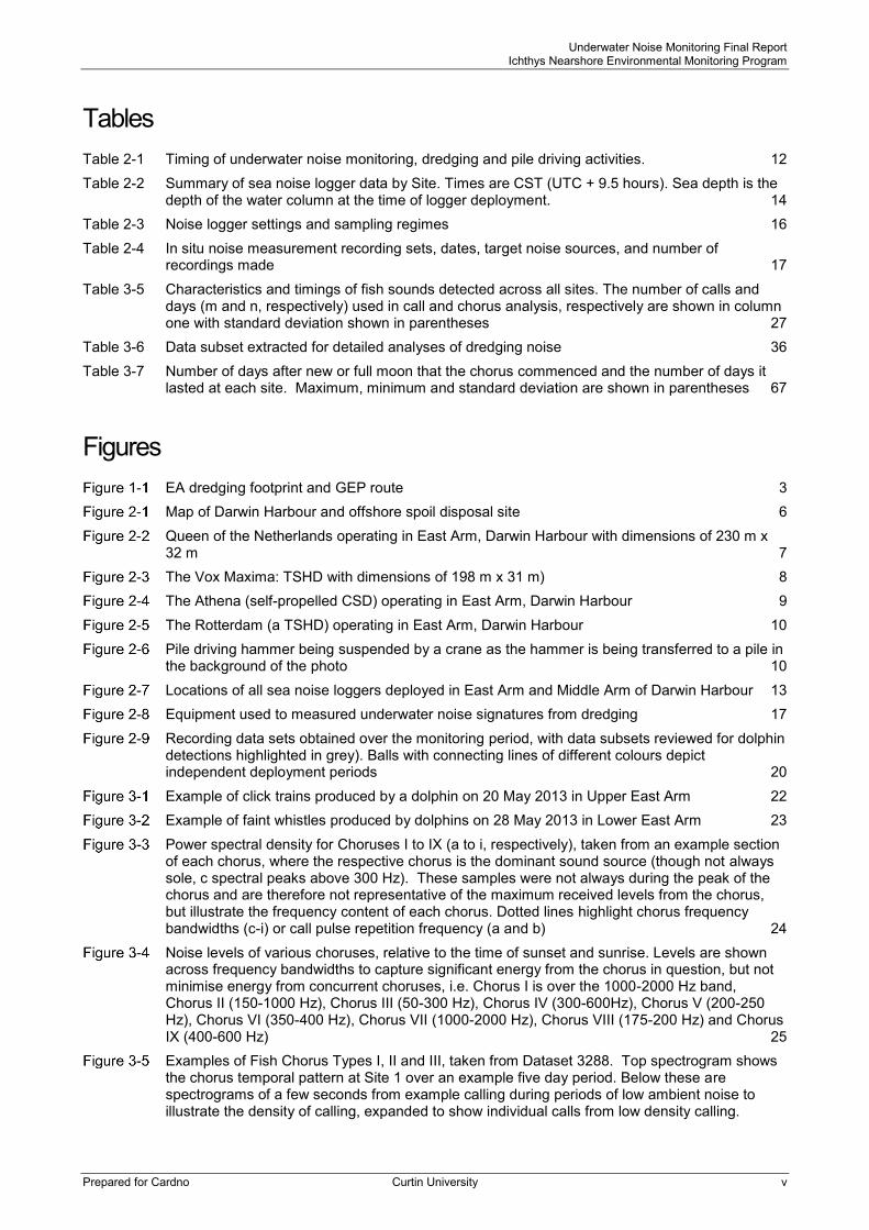
Tables Table 2-1 Timing of underwater noise monitoring, dredging and pile driving activities. 12
Table 2-2 Summary of sea noise logger data by Site. Times are CST (UTC + 9.5 hours). Sea depth is the depth of the water column at the time of logger deployment. 14
Table 2-3 Noise logger settings and sampling regimes 16
Table 2-4 In situ noise measurement recording sets, dates, target noise sources, and number of recordings made 17
Table 3-5 Characteristics and timings of fish sounds detected across all sites. The number of calls and days (m and n, respectively) used in call and chorus analysis, respectively are shown in column one with standard deviation shown in parentheses 27
Table 3-6 Data subset extracted for detailed analyses of dredging noise 36
Table 3-7 Number of days after new or full moon that the chorus commenced and the number of days it lasted at each site. Maximum, minimum and standard deviation are shown in parentheses 67
Figures EA dredging footprint and GEP route 3
Map of Darwin Harbour and offshore spoil disposal site 6
Queen of the Netherlands operating in East Arm, Darwin Harbour with dimensions of 230 m x 32 m 7
The Vox Maxima: TSHD with dimensions of 198 m x 31 m) 8
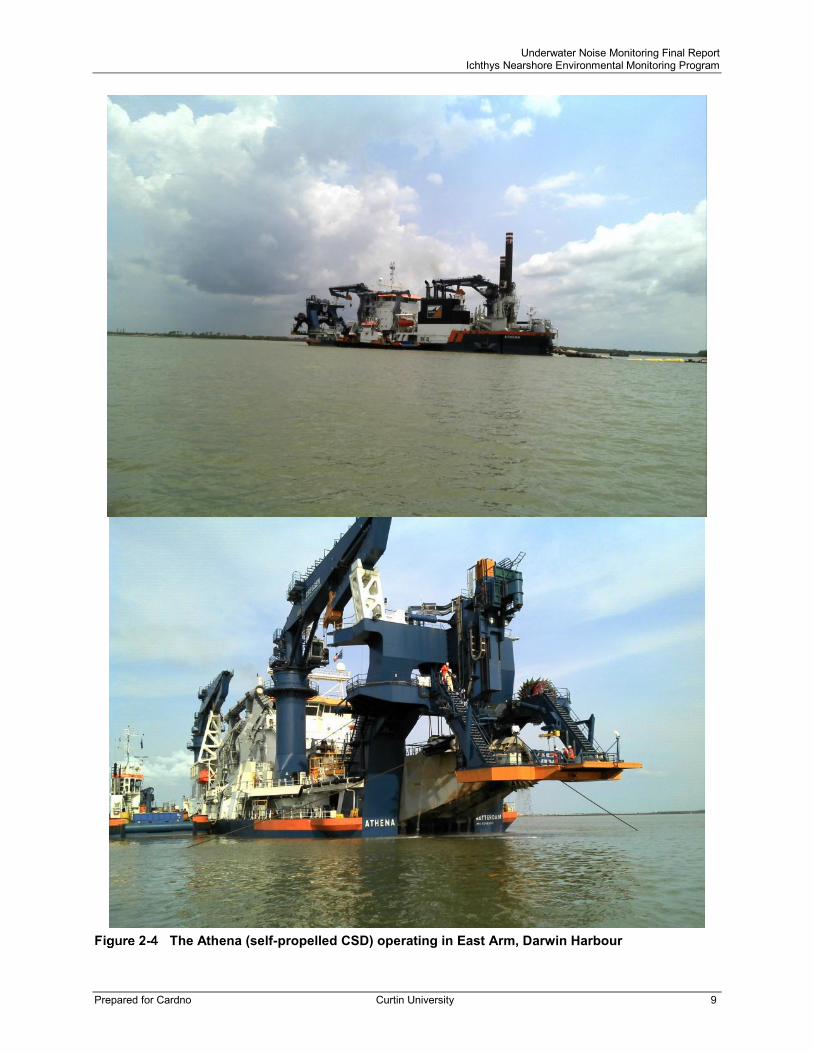
The Athena (self-propelled CSD) operating in East Arm, Darwin Harbour 9
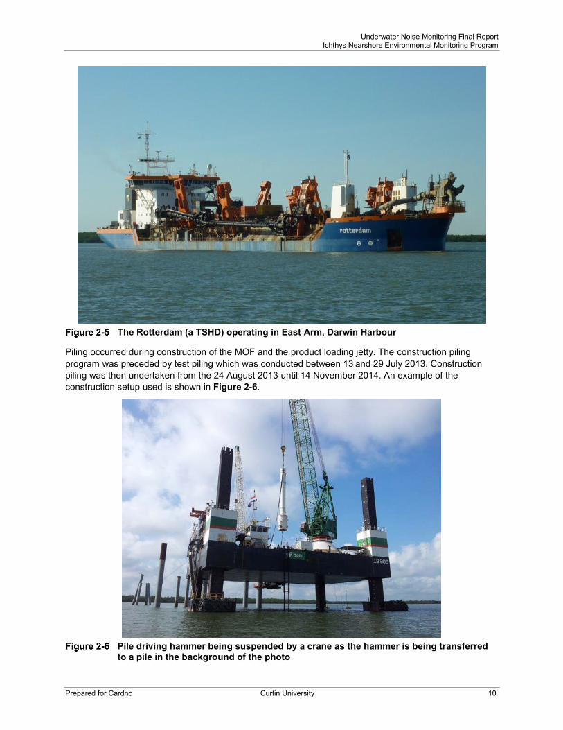
The Rotterdam (a TSHD) operating in East Arm, Darwin Harbour 10
Pile driving hammer being suspended by a crane as the hammer is being transferred to a pile in the background of the photo 10
Locations of all sea noise loggers deployed in East Arm and Middle Arm of Darwin Harbour 13
Equipment used to measured underwater noise signatures from dredging 17
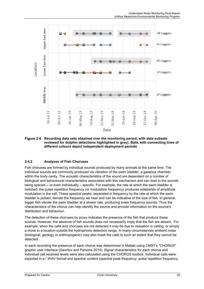
Recording data sets obtained over the monitoring period, with data subsets reviewed for dolphin detections highlighted in grey). Balls with connecting lines of different colours depict independent deployment periods 20
Example of click trains produced by a dolphin on 20 May 2013 in Upper East Arm 22
Example of faint whistles produced by dolphins on 28 May 2013 in Lower East Arm 23
Power spectral density for Choruses I to IX (a to i, respectively), taken from an example section of each chorus, where the respective chorus is the dominant sound source (though not always sole, c spectral peaks above 300 Hz). These samples were not always during the peak of the chorus and are therefore not representative of the maximum received levels from the chorus, but illustrate the frequency content of each chorus. Dotted lines highlight chorus frequency bandwidths (c-i) or call pulse repetition frequency (a and b) 24
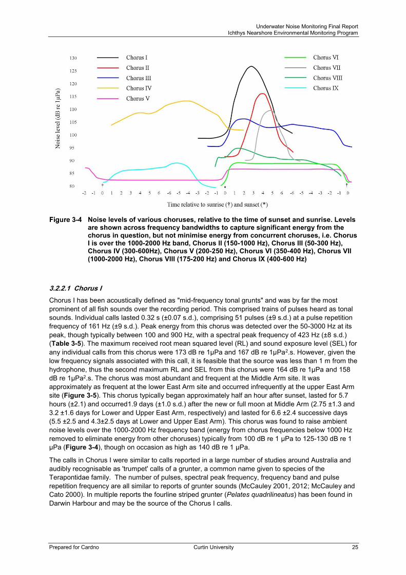
Noise levels of various choruses, relative to the time of sunset and sunrise. Levels are shown across frequency bandwidths to capture significant energy from the chorus in question, but not minimise energy from concurrent choruses, i.e. Chorus I is over the 1000-2000 Hz band, Chorus II (150-1000 Hz), Chorus III (50-300 Hz), Chorus IV (300-600Hz), Chorus V (200-250 Hz), Chorus VI (350-400 Hz), Chorus VII (1000-2000 Hz), Chorus VIII (175-200 Hz) and Chorus IX (400-600 Hz) 25
Examples of Fish Chorus Types I, II and III, taken from Dataset 3288. Top spectrogram shows the chorus temporal pattern at Site 1 over an example five day period. Below these are spectrograms of a few seconds from example calling during periods of low ambient noise to illustrate the density of calling, expanded to show individual calls from low density calling.

Underwater Noise Monitoring Final Report Ichthys Nearshore Environmental Monitoring Program
Prepared for Cardno Curtin University vi
Below these are the waveforms and expanded waveforms of the calls for Chorus I (left), II (middle) and III (right) 28
Examples of Fish Chorus Types IV, V and VI, taken from Datasets 3217, 3218 and 3221. Top spectrograms shows the chorus temporal pattern at Sites 1, 2 and 3 over an example five day period. Below these are spectrograms of a few seconds from example calling during periods of low ambient noise to illustrate the density of calling expanded to show individual calls from low density calling. Below these are the waveforms and expanded waveforms of the calls for Chorus IV (left), V (middle) and VI (right) 30
Examples of Fish Chorus Types VII, VIII and IX, taken from Dataset 3288. Top spectrogram shows the chorus temporal pattern at Site 1 over an example five day period. Below these are spectrograms of a few seconds from example calling during periods of low ambient noise to illustrate the density of calling expanded to show individual calls from low density calling. Below these are the waveforms and expanded waveforms of the calls for Chorus VII (left), VIII (middle) and IX (right) 32
Spectrograms for four different types of fish calls taken at various locations and times 34
Spectrogram of intense impulsive noise from snapping shrimp clearly seen by the red, vertical lines 35
Waveform of intense impulsive noise from snapping shrimp clearly seen by the red lines. Background noise in the absence of vessels is shown by the blue line 35
Locations of four sea noise loggers (red dots) deployed in East Arm of Darwin Harbour during the dredging operation in the Walker Shoal area. The area of dredging operation over the time period of dredging noise analysis is shown by the blue polygon 37
Long-time (500s) average spectrogram of underwater noise recorded by the LF logger near Walker Shoal from 9 to 12 November 2013 (top panel), and the sound pressure waveform of dredging noise from an individual 500-s recording (bottom panel) 38
Underwater noise level in a 20-1000 Hz frequency band (dashed line). The noise samples during the dredging operation of CSD Athena in the Walker Shoal area are indicated by red dots 39
Mean spectrum level of background underwater noise (dashed line) and percentiles of spectrum levels of dredging noise (colour lines) in 1/3-octave bands observed during the dredging operation of CSD Athena in the Walker Shoal area 39
Contours of received broadband sound pressure levels of underwater noise from a CSD dredger operating in the southern part of Walker Shoal (URS 2011) 40
Spectrogram showing intense noise from a vessel passing nearby 41
Waveform (left panel) and spectrogram (right panel) of intense broadband noise from a slowly moving vessel with the maximum received signal level of 149 dB re 1Pa 41
Example of broadband transport vessel superimposed on background dredging noise measured at a range of ~360 m. 42
Mean power spectrum density (PSD) of underwater noise measured by the LF logger between 2 November 2012 and 14 December 2012 in 1/3-octave frequency bands (±standard deviation) 43
Power spectrum density (PSD) of underwater noise with median, minimum and maximum levels in 1/3-octave frequency bands measured by the LF logger between 2 November 2012 and 14 December 2012 43
Spectrograms of sea noise recorded in Middle Arm using Low Frequency noise loggers over the first 18 months of the underwater noise measurement program 45
Spectrograms of sea noise recorded in Middle Arm using Low Frequency noise loggers over the last eight months of the underwater noise measurement program 46
Waveform (left panel) and spectrogram (right panel) at high time resolution of man-made noise recorded at 20:00 on the 24 June 2014 on LF 3322 46
Spectrograms of sea noise recorded over the two year period in Lower East Arm with Low Frequency noise loggers 48
Spectrogram of intense man-made noise between the 23 April and the 30 April 2013 49
Underwater Noise Monitoring Final Report Ichthys Nearshore Environmental Monitoring Program
Prepared for Cardno Curtin University vii
Spectrograms of sea noise recorded over the two year period in Upper East Arm over the first 15 months of the underwater noise measurement program (note: scale of the bottom, left spectrogram differs from scales of other spectrograms due to a variation in logger settings). 50
Spectrograms of sea noise recorded in Upper East Arm over the 16th to the 18th month (Aug-Nov 2014) of the underwater noise measurement program 51
Spectrograms of sea noise recorded in Upper East Arm over the last 3 months of the underwater noise measurement program 52
High frequency (top panel) and low frequency (middle panel) long-term average spectrograms of sea noise recorded on an HF logger over a 10-day period between 15 December and 25 December 2012. The bottom panels show the waveform (left) and spectrogram (right) of continuous broadband noise, likely from dredging 53
Pile driving (upper panels) and dredging noise (lower panels) waveforms (left panels) and spectrograms (right panels) from recordings on the 16 and 17 May 2014 54
Underwater recording data subsets reviewed for dolphin detections over the monitoring period, with dolphin detections indicated with a red cross. Balls with connecting lines of different colours depict independent deployment periods (lasting approximately 2 to 3 months each) 56
Presence and qualitative split of relative intensity of Chorus I for the Middle Arm, Lower East Arm and Upper East Arm (Sites 1,2 and 3 respectively – Site 4 provided an alternate Upper Middle Arm recording for the first two months only) across all recording periods 58
Presence and qualitative split of relative intensity of Chorus II for the Middle Arm, Lower East Arm and Upper East Arm (Sites 1,2 and 3 respectively – Site 4 provided an alternate Upper Middle Arm recording for the first two months only) across all recording periods 59
Presence and qualitative split of relative intensity of Chorus III for the Middle Arm, Lower East Arm and Upper East Arm (Sites 1,2 and 3 respectively) across all recording periods 60
Presence and qualitative split of relative intensity of Chorus IV for the Middle Arm, Lower East Arm and Upper East Arm (Sites 1,2 and 3 respectively) across all recording periods 61
Presence and qualitative split of relative intensity of Chorus V for the Middle Arm, Lower East Arm and Upper East Arm (Sites 1, 2 and 3 respectively) across all recording periods 62
Presence and qualitative split of relative intensity of Chorus VI for the Middle Arm, Lower East Arm and Upper East Arm (Sites 1, 2 and 3 respectively) across all recording periods 63
Presence and qualitative split of relative intensity of Chorus VII for the Middle Arm, Lower East Arm and Upper East Arm (Sites 1, 2 and 3 respectively) across all recording periods 64
Presence and qualitative split of relative intensity of Chorus VIII for the Middle Arm, Lower East Arm and Upper East Arm (Sites 1, 2 and 3 respectively) across all recording periods 65
Presence and qualitative split of relative intensity of Chorus IX for the Middle Arm, Lower East Arm and Upper East Arm (Sites 1, 2 and 3 respectively) across all recording periods 66
Trading vessels visiting Darwin Harbour in 2011/12, 2012/13, 2103/14 and 2014/15 (data from: Port of Darwin Trade Report 2015) 69
Appendices Appendix A Reference Systems and Acoustic Units

Underwater Noise Monitoring Final Report Ichthys Nearshore Environmental Monitoring Program
Prepared for Cardno Curtin University 1
1 Introduction
1.1 Overview INPEX is the operator of the Ichthys LNG Project (the Project). The Project comprises the development of offshore production facilities at the Ichthys Field in the Browse Basin, some 820 km west-south-west of Darwin, an 889 km long subsea gas export pipeline (GEP) and an onshore processing facility and product loading jetty at Bladin Point on Middle Arm Peninsula in Darwin Harbour. To support the nearshore infrastructure at Bladin Point, dredging works were carried out to extend safe shipping access from near East Arm Wharf to the new product loading facilities at Bladin Point, which are supported by piles driven into the sediment (Figure 1-1). A trench was also dredged to seat and protect the GEP for the Darwin Harbour portion of its total length. Dredged material was disposed at the spoil ground located approximately 12 km north-west of Lee Point. A detailed description of the dredging and spoil disposal methodology is provided in Section 2 of the East Arm (EA) Dredging and Spoil Disposal Management Plan (DSDMP) (INPEX 2013) and GEP DSDMP (INPEX 2014a).
1.2 Background The Project was assessed by the Department of the Environment, Water, Heritage and the Arts (DEWHA) as having the potential to cause a significant impact on Environmental Protection and Biodiversity Conservation Act 1999 (EPBC Act) protected matters, an Environmental Impact Statement (EIS) was prepared to satisfy the requirements from both the Commonwealth and the Northern Territory Governments. A component of the EIS identified potential impacts from nearshore infrastructure development including the dredging of a trench to seat and protect the GEP within Darwin Harbour, dredging to extend safe shipping access from near East Arm Wharf to the new product loading facilities at Bladin Point, and the installation of piles for supporting the new facility (in particular a Module Offloading Facility (MOF) and a long jetty) (Figure 1-1).
The works also include the disposal of dredged material at a spoil ground located approximately 12 km north-west of Lee Point (Figure 2-1). A detailed description of the proposed dredging and spoil disposal methodology is provided in Section 2 of the Dredging and Spoil Disposal Management Plan – East Arm (DSDMP) (INPEX 2013).
In the draft EIS (INPEX 2010), the production of underwater noise was identified as one of several potential environmental impacts from the nearshore component of the Project. Substantial underwater noise was predicted to be produced during activities associated with construction, including dredging, pile driving and overall increased vessel activity. A protracted drilling and blasting program was originally proposed and was identified as the source producing the most significant underwater noise. Blasting and drilling were considered to have the highest risk of direct injuries to fauna. However, alternatives to drilling and blasting were identified during subsequent stages of the Project and these works were not implemented.
Nonetheless, impacts from intense and/or prolonged noise from pile driving, dredging and increased shipping were still identified as having a potential to cause impacts, with overall underwater noise in the environment anticipated to increase above previous levels of ambient noise. Key species identified as potentially experiencing impacts from underwater noise included three species of coastal dolphins (bottlenose, Indo-pacific humpback and snubfin dolphins), dugongs, marine turtles (green, hawksbill, flatback and olive ridley) and fish.
In the assessment of underwater noise impacts to these species, a range of effects were considered including injury and hearing loss (permanent and temporary threshold shifts) as the most severe (Appendix 15 of the Draft EIS; URS 2009). Masking, stress and behavioural responses were also considered as responses to noise impacts. Behavioural responses such as avoidance or disruption of foraging or resting; masking of important signals such as echolocation signals, intra-species communication, and predator-prey cues and increased stress were identified as potentially occurring from lower level noise exposure. However, if the exposure is significant (either because of its long duration, high frequency, high intensity or a

Underwater Noise Monitoring Final Report Ichthys Nearshore Environmental Monitoring Program
Prepared for Cardno Curtin University 2
combination of these), these responses could result in abandonment of habitats or a decline in health of individuals or the population.
The draft EIS considered the fact that fauna have different levels of sensitivity to underwater noise. Cetaceans, for example, are particularly sensitive to sound since they depend upon sound to create an image of the environment through echolocation, to communicate with conspecifics (other animals of the same species) and to detect predators. The low visibility within Darwin Harbour’s naturally turbid waters means that animals likely depend heavily on sound and to a lesser extent sight. Some fish are more sensitive to sound than others and many use sound to broadcast choruses for attraction and competition amongst conspecifics for reproductive purposes.
Due to the varied levels of sensitivities among species, as well as the range in impact severity, mitigation was implemented based on what was considered to be the most severe of these effects – that is, thresholds required to cause hearing threshold shifts for key marine faunal groups (adopted from Southall et al. 2007). To map the predicted underwater noise footprint that could cause these more severe effects, INPEX conducted modelling to predict sound levels with range from key noise sources. The details of the model results are described in the EIS Supplement (INPEX 2011).
Overall, the modelling suggested that the risks of significant direct impacts to marine fauna from underwater noise produced by pile driving and dredging were predicted to be relatively low. However, there was a risk identified associated with direct and indirect behavioural changes, masking and stress responses from multiple sources and long-term noise exposure. Noise-generating activities were predicted to likely provoke avoidance of the impacted area over a sustained period. Specifically, the EIS Supplement indicated that the ‘underwater noise environment of East Arm was predicted to become a challenging environment for marine fauna, particularly the coastal dolphin species, and that it is presumed that these species will be excluded from the Eastern part of Darwin Harbour for an extended period during construction’ (INPEX 2011).
As such, a Nearshore Environmental Monitoring Plan (NEMP; Cardno 2014) was developed, which included the direct monitoring of marine fauna (e.g. turtles and dugongs) to assess potential changes in abundance and distribution as a result of construction activities. Indirect monitoring programs, including underwater noise, were also included to inform whether potential changes in fauna were attributable to Project construction activities.

Underwater Noise Monitoring Final Report Ichthys Nearshore Environmental Monitoring Program
Prepared for Cardno Curtin University 3
EA dredging footprint and GEP route

Underwater Noise Monitoring Final Report Ichthys Nearshore Environmental Monitoring Program
Prepared for Cardno Curtin University 4
1.3 Objectives The aim of the Underwater Noise Monitoring Program is to monitor and report on the effects of the Project’s construction (dredging and piling) activities on the underwater noise environment in Darwin Harbour. Key objectives of the Underwater Noise Monitoring Program include:
> Establish underwater noise characteristics at selected locations within Darwin Harbour prior to the commencement of, during, and following the completion of dredging and piling in East Arm. The data should be suitable to inform the assessment of changes in abundance and distribution of dolphins, turtles, dugongs and fish that may be observed during and after the main noise-generating activities associated with the marine construction activities, and
> Validate the modelling of CSD dredging, and of piling, undertaken as part of the EIS Supplement studies (see Appendix S7 of INPEX 2011).
- Test the conservatism of the assumptions used in the model.
- Consider whether it is warranted to feasible to modify the radius of the marine fauna observation zone around piling operations (as predicted in Appendix S7 of INPEX 2011)
To verify the underwater noise models, in situ measurements of underwater noise emitted from dredging and pile driving operations were undertaken. However, only measurements of dredging are reported on here. Pile driving measurements are reported in a separate monitoring program (INPEX 2014b).
As part of the long-term underwater noise monitoring program, biological, physical, and anthropogenic noise in Darwin Harbour was measured over a two year period, from the beginning of the Project (November 2012) to several months after dredging and marine pile driving works had been completed (January 2015) using deployed, stationary autonomous sea noise recorders (hereinafter referred to as noise loggers). Noise loggers were deployed at Middle and East Arms, to represent locations away from the construction activity and within the vicinity of the construction activities respectively. As a result, spatial and temporal changes in underwater noise inside and outside the development activity area were measured.
In summary, the specific objectives of this report are to:
> Quantify and describe noise from major physical, anthropogenic (main emphasis on dredging, machinery, vessel), and biological sources, and
> Compare the dominant sources of underwater noise in the soundscape of Middle Arm and East Arm over the measurement period.
> Compare dredging underwater noise levels measured during construction with EIS model predictions

Underwater Noise Monitoring Final Report Ichthys Nearshore Environmental Monitoring Program
Prepared for Cardno Curtin University 5
2 Methodology
2.1 Location Darwin Harbour is a large tropical embayment approximately 500 km2 in extent. Freshwater flows into Darwin Harbour in abundance during the wet season between November and April. The area experiences little rain during the dry season between May and October. The harbour has three arms: East, Middle (the largest and longest) and West (the smallest) (Figure 2-1). Each arm is surrounded by extensive mangrove systems and intertidal mud flats. Darwin Harbour experiences a maximum tide of 7.8 m, with a mean neap tide height ranging from 3.2 m to 5.0 m (mean low water neap to mean high water neap) and a mean spring tide height ranging from 1.3 m to 7.0 m (mean low water spring to mean high water spring, taken from Geoscience Australia’s chart AUS00026). Water depths in the central embayment area vary generally between 15 m and 25 m (above chart datum). In the central East Arm west of 130° 54’ E, depths vary between 10 m and 15 m, although there are extensive shallow areas bordering the central channel of 1 m to 5 m depth (above chart datum). In East Arm, east of 130° 54’ E, the water shoals from 3 m to 7 m above chart datum. The high tide range combined with long and comparatively narrow arms results in strong tidal currents of up to 2 m/s (Padovan, 1997; Talbot, 2006)..
The harbour is known to have an abundance of marine wildlife, including more than 415 species of fish (Larson and Williams 1997), 26 reptiles (including crocodiles, 20 species of seasnakes and 5 species of marine turtles – green, hawksbill, loggerhead, olive ridley and flatback), dugongs, and three species of regularly sighted dolphins (bottlenose, Indo-Pacific Humpback and snubfin dolphins (Department of Land Resource Management 2015a, 2015b). In addition to the four marine mammals that occur regularly, other species of marine mammals may visit occasionally (Chatto and Warneke 2000).
The Port of Darwin is also in a strategic geographical position being Australia’s nearest port to the growing Asian economies and the northern terminus of the AustralAsia Railway’s junction of East Arm Wharf to the national rail system. The Port has the capacity to berth, moor and service a range of vessel types. Vessels can use one of five wharfs and one mooring basin, depending upon the type and requirement of the vessel. The largest of the wharves is the East Arm Wharf, which is the principal location for import and export and handles bulk ores and liquids, live cattle, cement clinker, rig tenders, vehicle imports and general cargo and containers. Fort Hill Wharf has restricted access and handles cruise ships, custom vessels, naval vessels, tug boats and pilot vessels. Stokes Hill Wharf is an area of historic attraction used for tourism and has access for recreational and fishing vessels. The Frances Bay Fishing Harbour Mooring Basin is accessed via a lock (allowing access during most tides) and handles private and recreational vessels as well as the northern fishing fleet of prawn, fishing and pearling vessels. Hornibrook’s Wharf is used by local commercial operators including the local barramundi fishery.

Underwater Noise Monitoring Final Report Ichthys Nearshore Environmental Monitoring Program
Prepared for Cardno Curtin University 6
Map of Darwin Harbour and offshore spoil disposal site

Underwater Noise Monitoring Final Report Ichthys Nearshore Environmental Monitoring Program
Prepared for Cardno Curtin University 7
2.2 Dredging and Pile Driving Sources Dredging was necessary at various locations within Darwin Harbour to allow the extension of the existing shipping channel from near East Arm Wharf to the product loading jetty at Bladin Point, a turning basin for ships, two berthing pockets at the product loading jetty, an approach apron and berthing pocket at the MOF and a trench for the subsea GEP to Middle Arm Peninsula.
The dredging program required a range of dredging vessel, including a trailing suction hopper dredgers (TSHDs), a cutter suction dredger (CSD), backhoe dredgers (BHDs) and split hopper barges (SHBs). The CSD targeted more-consolidated material, including Walker Shoal. The dredged spoil was transported to the offshore spoil disposal ground outside Darwin Harbour.
Season One of the East Arm dredging campaign commenced on 27 August 2012 with BHDs, with the CSD commencing on 4 November 2012, with all Season One dredging operations ceasing on 30 April 2013. The ‘dry season’ dredging hiatus extended from 1 May 2013 to 31 October 2013. Season Two of the East Arm dredging campaign commenced on 1 November 2013 and ceased on 11 June 2014, while the GEP dredging program commenced on 23 October 2013 and concluded on 12 July 2014.
Some of the dredges used during the Project include: the Queen of the Netherlands (TSHD), the Athena (CSD), the Vox Maxima (TSHD) and the Rotterdam (TSHD) (see Figure 2-2 to Figure 2-5).
Queen of the Netherlands operating in East Arm, Darwin Harbour with dimensions of
230 m x 32 m

Underwater Noise Monitoring Final Report Ichthys Nearshore Environmental Monitoring Program
Prepared for Cardno Curtin University 8
The Vox Maxima: TSHD with dimensions of 198 m x 31 m)
Underwater Noise Monitoring Final Report Ichthys Nearshore Environmental Monitoring Program
Prepared for Cardno Curtin University 9
The Athena (self-propelled CSD) operating in East Arm, Darwin Harbour
Underwater Noise Monitoring Final Report Ichthys Nearshore Environmental Monitoring Program
Prepared for Cardno Curtin University 10
The Rotterdam (a TSHD) operating in East Arm, Darwin Harbour
Piling occurred during construction of the MOF and the product loading jetty. The construction piling program was preceded by test piling which was conducted between 13 and 29 July 2013. Construction piling was then undertaken from the 24 August 2013 until 14 November 2014. An example of the construction setup used is shown in Figure 2-6.
Pile driving hammer being suspended by a crane as the hammer is being transferred
to a pile in the background of the photo

Underwater Noise Monitoring Final Report Ichthys Nearshore Environmental Monitoring Program
Prepared for Cardno Curtin University 11
2.3 Underwater Sound Recording
2.3.1 Stationary Measurements
Forty-two sea noise loggers were strategically deployed in Darwin Harbour between 2 November 2012 and 15 January 2015 to capture long-term ambient noise away from and in the vicinity of construction activities (Table 2-1; Table 2-2).
Loggers deployed in Middle Arm had little influence from noise produced by construction activities, while those in East Arm were placed within proximity to Project construction activities. One deployment location was selected in West Arm, while two locations (at any one time) were selected in East Arm (one upstream and one downstream). The two loggers in East Arm were repositioned slightly over the monitoring period so that they did not interfere with construction activities. The exact locations of all logger deployment locations are shown on the map in Figure 2-7 and Table 2-2, and the sea depths at the deployment locations and the time periods of recordings are presented in Table 2-2. Hydrophones were attached on the external housing of the noise loggers which were set on the seafloor.
Both low frequency (LF) and high frequency (HF) loggers were deployed during noise monitoring. The LF sea noise loggers were designed and built at the CMST. HF loggers were of two types. One was assembled at the CMST using an HTI hydrophone, an impedance matching pre-amplifier (same as that used in the LF logger) and a programmable 16-bit digital data recorder made by Wildlife Acoustics Inc. The second HF logger was an SM2M underwater sound recorder from Wildlife Acoustics Inc. All three logger types were programmed to make continuous recordings of a fixed length (see Table 2-3), repeating every 900 seconds. Sampling rates and anti-aliasing filter settings for all loggers are given in Table 2-3.

Underwater Noise Monitoring Final Report Ichthys Nearshore Environmental Monitoring Program
Prepared for Cardno Curtin University 12
Table 2-1 Timing of underwater noise monitoring, dredging and pile driving activities. Activity 2012 2013 2014 2015
Nov Dec Jan Feb Mar Apr May Jun Jul Aug Sep Oct Nov Dec Jan Feb Mar Apr May Jun Jul Aug Sep Oct Nov Dec Jan Feb
Noi
se
Mon
itorin
g Middle Arm East Arm (Lower Reaches) East Arm (Upper Reaches)
Dev
elop
men
t Act
iviti
es
Dredging (BHD)
Dredging (CSD) Dredging (TSHD)
Piling (Test) Piling (Construction)

Underwater Noise Monitoring Final Report Ichthys Nearshore Environmental Monitoring Program
Prepared for Cardno Curtin University 13
Locations of all sea noise loggers deployed in East Arm and Middle Arm of Darwin Harbour

Underwater Noise Monitoring Final Report Ichthys Nearshore Environmental Monitoring Program
Prepared for Cardno Curtin University 14
Table 2-2 Summary of sea noise logger data by Site. Times are CST (UTC + 9.5 hours). Sea depth is the depth of the water column at the time of logger deployment.
Deployment ID
Logger Dataset No.
Latitude (S)
Longitude (E)
Sea depth
(m) Start and end of recording in water (WST)
No. of recordings
Middle Arm Site
1 LF Logger 1 (3164) 12° 32.873’ 130° 50.753’ 12 2-Nov 2012 11:00 to 2-Feb
2013 12:45 8857
2 LF Logger 1 ( 3178) 12° 32.876' 130° 50.728' 15 04-Apr 2013 12:00 to 05-Jun
2013 12:45 5934
3 LF Logger (3217) 12° 32.881’ 130° 50.752’ 15 7 Jun 2013 17:30 to 11 Sep
2013 23:30 9197
4 LF Logger (3237) 12° 32.895’ 130° 50.756’ 15 13 Sep 2013 16:00 to 11
Nov 2013 23:45 5756
5 LF Logger (3259) 12° 32.865' 130° 50.732' 15 13 Nov 2013 08:30 to 10 Feb
2013 23:15 8698
6 LF Logger (3288) 12° 32.888' 130° 50.752' 15 11 Feb 2014 10:30 to 1 May
2014 09:45 8764
7 LF Logger (3322) 12° 32.875’ 130° 50.741’ 15 10 May 2014 10:00 to 9 Aug
2014 02:45 8747
8 LF Logger (3337) 12° 32.910’ 130° 50.759’ 15 9 Aug 2014 14:30 to 19 Nov
2014 12:45 9796
9 LF Logger (3366) 12° 32.933’ 130° 50.775’ 15 19 Nov 2014 14:30 to 15 Jan
2015 08:45 5468
Lower Reaches of East Arm (Western Site towards the mouth)
10 LF Logger (3163) 12°29.827' 130°52.404' 12 2-Nov 2012 10:45 to 13-Dec
2012 15:15 3955
11 LF Logger 2 (3166) 12° 29.804' 130° 52.404' 15 14-Dec 2012 8:00 to 9-Mar
2013 3:15 8142
12 LF Logger 2 (3179) 12° 29.832' 130° 52.428' 12 03-Apr 2013 14:30 to 05-Jun
2013 09:30 5969
13 HF Logger 1 (3180) 12° 29.832' 130° 52.428' 12 03-Apr 2013 14:30 to 05-Jun
2013 07:30 6047
14 HF Logger (3218) 12° 29.836' 130° 52.400' 12 7 Jun 2013 17:30 to 6 Sep
2013 19:00 9208
15 LF Logger (3220) 12° 29.836' 130° 52.400' 12 7 Jun 2013 17:30 to 11 Sep
2013 23:30 9204
16 LF Logger (3236) 12° 29.828' 130° 52.405' 12 18 Sep 2013 12:00 to 11
Nov 2013 23:45 4935
17 HF Logger (3240) 12° 29.828' 130° 52.405' 12 18 Sep 2013 18:00 to 12
Nov 2013 18:45 5736
18 LF Logger (3258) 12° 30.152’ 130° 53.859’ 5 12 Nov 2013 17:30 to 10 Feb
2014 23:15 Unrecovered
19 HF Logger (3260) 12° 30.152’ 130° 53.859’ 5 12 Nov 2013 09:30 to 10 Feb
2014 23:15 Unrecovered
20 LF Logger (3289) 12° 30.187' 130° 54.213' 5 - Failed
21 LF Logger (3289-2) 12° 30.108' 130° 54.705' 9 - Failed

Underwater Noise Monitoring Final Report Ichthys Nearshore Environmental Monitoring Program
Prepared for Cardno Curtin University 15
Deployment ID
Logger Dataset No.
Latitude (S)
Longitude (E)
Sea depth
(m) Start and end of recording in water (WST)
No. of recordings
22 HF Logger (3291) 12° 30.187' 130° 54.213' 5 11 Feb 2014 10:00 to 14 Mar
2014 17:15 8801
23 HF Logger (3291-2) 12° 30.108' 130° 54.705' 9 11 Feb 2014 10:00 to 10
May 2014 17:15 8801
24 LF Logger (3323) 12° 29.853’ 130° 52.444’ 12 10 May 2014 07:00 to 8 Aug
2014 16:45 8671
25 HF Logger (3324) 12° 29.853’ 130° 52.444’ 12 10 May 2014 14:30 to 9 Aug
2014 16:30 8650
26 LF Logger (3238) 12° 30.149' 130° 53.860' 5 18 Sep 2013 16:00 to 11
Nov 2013 23:45 5743
27 HF Logger (3339) 12° 29.857’ 130° 52.408’ 12 9 Aug 2014 13:30 to 19 Nov
2014 09:45 9778
28 HF Logger (3368) 12° 29.858’ 130° 52.412’ 12 18 Nov 2014 17:30 to 15 Jan
2015 08:45 5556
Upper Reaches of East Arm (Eastern Site )
29 HF Logger 1 (3165) 12°30.617’ 130°54.022’ 13 1-Nov 2012 18:15 to 3-Nov
2012 18:00 195
30 LF Logger ( 3196) 12° 30.664' 130° 53.958' 15 14-Dec 2012 16:00 to 11-Apr
2013 10:15 9711
31 LF Logger 3 (3202) 12° 30.200' 130° 53.671' 5 03-Apr 2013 10:30 to 05-Jun
2013 06:00 6004
32 HF Logger 2 (3181) 12° 30.200' 130° 53.671' 5 03-Apr 2013 10:30 to 05-Jun
2013 06:15 6043
33 HF Logger (3219) 12° 30.187' 130° 53.851' 5 7 Jun 2013 19:00 to 6 Sep
2013 23:30 9188
34 LF Logger (3221) 12° 30.187' 130° 53.851' 5 7 Jun 2013 17:30 to 11 Sep
2013 23:30 9194
35 HF Logger (3239) 12° 30.149' 130° 53.860' 5 19 Sep 2013 09:30 to 12
Nov 2013 23:45 5265
36 LF Logger (3257) 12° 29.825' 130° 52.408' 12 12 Nov 2013 17:30 to 10 Feb
2014 23:15 8689
37 HF Logger (3261) 12° 29.825' 130° 52.408' 12 13 Nov 2013 08:00 to 10 Feb
2014 23:15 Failed
38 HF Logger (3325) 12° 30.130' 130° 54.724' 5 17 May 2014 09:15 to 9 Aug
2014 09:00 8723
39 HF Logger (3338) 12° 30.127’ 130° 54.703’ 5 9 Aug 2014 13:31 to 19 Nov
2014 10:32 9781
40 HF Logger (3369) 12° 30.127' 130° 54.748' 5 19 Nov 2014 13:30 to 15 Jan
2015 13:00 5473
41 LF Logger (3367) 12° 30.127' 130° 54.748' 5 18 Nov 2014 17:30 to 15 Jan
2015 13:30 5557
Upper Reaches of East Arm (Eastern Site 2)
42 HF Logger 2 (3162) 12° 29.783' 130° 55.174' 12 2-Nov 2012 10:00 to 13-dec
2012 12:00 3944

Underwater Noise Monitoring Final Report Ichthys Nearshore Environmental Monitoring Program
Prepared for Cardno Curtin University 16
Table 2-3 Noise logger settings and sampling regimes
Logger Dataset # Gain (ch.1/ch.2,
dB)
Sample Rate/Anti-aliasing
Filter (kHz)
Duty Cycle
LF Logger (3163) 20/40 11/4.5 350 s every 900 s
HF Logger (3165) 32/56 96/45 300 s every 900 s
HF Logger (3162) 20/44 96/45 300 s every 900s
HF Logger (3196) 20/44 48/23 120 s every 900 s
LF Logger (3164) 20/40 11/5 350 s every 900 s
LF Logger (3166) 20/40 11/5 350 s every 900 s
HF Loggers (3180, 3181, 3218, 3219, 3239, 3240, 3260, 3261, 3290, 3291-1, 3291-2, 3324, 3325) 44 96/45 250 s every 900 s
HF Loggers (3324, 3338) 44 96/45 250 s every 900 s
LF Loggers (3178, 3179, 3202, 3217, 3220, 3221, 3236,3237, 3238, 3257, 3258, 3259, 3287, 3288, 3289-1, 3289-2, 3322, 3323, 3337, 3366)
40 12/5.5 500 s every 900 s
HF Logger (3339) 54 96/45 250 s every 900 s
LF Logger (3367) 20/40 11/4.5 350 s every 900 s
HF Logger (3369) 32 96/45 250 s every 900 s
The frequency response of all noise loggers assembled at CMST was calibrated with respect to the input voltage of the analogue-to-digital converter (ADC) per 1 Pa at the hydrophone before deployment by inputting white noise of a known level in series with the hydrophone and then correcting the recorded signal for the hydrophone sensitivity. The frequency responses of loggers are presented in the field reports (Gavrilov and Salgado Kent 2015, Salgado Kent et al. 2015, Parsons et al. 2014, Salgado Kent and McCauley 2014, Salgado Kent et al. 2014a, Salgado Kent et al. 2014b, Marley et al. 2013, McCauley et al. 2013, Salgado Kent et al. 2013,).
The SM2M sea noise recorder does not have any calibration circuit (or capability) and hence the frequency response of SM2M was determined based on the calibrated hydrophone sensitivity of -163.7 dB re V/µPa, the total recording system gain and the ADC conversion rate in number of bits per 1 Volt.
2.3.2 In Situ Measurements
The in situ measurements involved lowering of a hydrophone over the side of a small vessel to measure underwater noise generated from specific activities. By using this technique, measurements could be made at various ranges and azimuths (to account for any source directionality) from the source. Measurements were made to estimate source levels (equivalent source level at 1 m range if it were assumed to be a point source) and verify predicted noise levels used in assessing environmental impacts.
Small vessel measurements were made three times during the underwater noise monitoring program; once at the beginning of the program in December 2012, once in February 2013, and once in August 2014 (Table 2-4). Recording sets were made during dredging and pile driving activities.

Underwater Noise Monitoring Final Report Ichthys Nearshore Environmental Monitoring Program
Prepared for Cardno Curtin University 17
Table 2-4 In situ noise measurement recording sets, dates, target noise sources, and number of recordings made
Recording Sets
Dates Noise Source Targeted No. of Recordings
1 14 December 2012 to 15 December 2012 Dredging 24
2 9 February 2013 to 10 February 2013 Dredging and Pile Driving 34
3 7 August 2014 Pile Driving 13
Recordings were made by lowering the hydrophone to approximately 4 to 7 m depth over the side of the boat and at tidal heights (above Prediction Datum) between 0.3 m and 6 m. Bushnell laser range finding binoculars (eye safe with a maximum range of 400 m) and a hand held GPS with a compass were used to obtain the positional information of the dredgers (at approximately the middle point of the length of the dredgers) and pile being driven.
The measurements were made with a SoundDevices 744T digital recorder using 24 bit samples and 48 kHz or 96 kHz sample rate with gain varied to suit the signal level (hard set; Figure 2-8). The hydrophone was a Reson TC4033 with a Reson VP 1000 pre-amplifier, with gain (a setting on the pre-amplifier) set to suit the signal level (adjustable gain from 0 dB to 32 dB in 6 dB steps).
Equipment used to measured underwater noise signatures from dredging
The recording system was calibrated after the measurements were taken by inputting white noise of known level in series with the hydrophone and then correcting the measured voltage for the hydrophone sensitivity, which was -202.6 dB re 1V/Pa. The frequency responses of the recording system (system gain) are shown in the field reports (Gavrilov et al. 2012, 2015; Salgado Kent et al. 2014c). The measured sea noise waveform and spectrum levels were corrected for the system’s frequency response in the analyses.

Underwater Noise Monitoring Final Report Ichthys Nearshore Environmental Monitoring Program
Prepared for Cardno Curtin University 18
2.4 Data Analysis Processing and analysis of sea noise data involved two stages:
1. The power spectral density (PSD) of sea noise (or noise spectrum) was calculated for each recording. The recording channel of higher gain was selected if the signal was not clipped by the ADC dynamic range; otherwise, the low-gain channel was used. The PSD was corrected for the frequency response of the acoustic recording system derived from the calibration data and from the hydrophone sensitivity, so that the noise spectra and spectral levels represented absolute values (Pa2/Hz and dB re 1 Pa2/Hz, respectively). These spectra were used to plot long-term average spectrograms of sea noise. Such spectrograms were then used to visually review the main features of sea noise and their long-term variations in the second stage of data analysis; and
2. A Matlab toolbox with a Graphic User Interface was developed to: a) visualise sea noise spectrograms of low temporal resolution (long-term average spectrograms) for a chosen time period of several days; b) select particular recording times based on the spectrogram features of interest; and c) analyse the waveform and spectrogram of sea noise within the individual recording made at the selected time. During this stage the time-frequency characteristics of sea noise was investigated in more detail using spectrograms of high resolution. Moreover, a de-spiking filter and low- and high-pass filtering was applied to the noise signal to reduce the effect of snapping shrimp noise and to extract signals of interest (e.g. dolphin clicks and whistles). An auto-regression method was used to locate impulses of snapping shrimp noise, and to remove these impulses and interpolate the signal waveform within the resulting gaps. Such an approach to signal de-noising allows the preservation of spectral characteristics of other noises recorded on the logger. Because the de-spiking procedure is computationally heavy (demanding a large amount of RAM) it was not applied to the whole dataset.
Acoustic units used for sea noise analysis and referred to in this report are described in Appendix A.
For the purposes of this report, long-term average spectrograms of sea noise obtained from the signal PSDs averaged over each individual recording were created with each panel representing time periods of ten days to visually examine the noise data for long-term variations. The spectrograms are displayed with a logarithmic frequency scale and a fixed colour scale bounded within 50 dB and 90 to 130 dB re 1 Pa2/Hz. The spectrograms of the LF logger data have a frequency scale from 5 Hz to 5000 Hz, while the HF logger data are split into two bandwidths: one in the lower frequency range from 20 Hz to 1000 Hz and the other in the range of 1 kHz to 46 kHz.
These spectrograms demonstrate broad-scale temporal patterns only and, because of the averaging involved, do not display individual signals that are short compared with the averaging time. The spectrograms tend to highlight signal types that are intense and/or persist across the averaging time (e.g. intense ship or dredging noise).
An analysis of higher temporal resolution was undertaken for selected recordings to demonstrate typical signals at monitored sites.
2.4.1 Semi-automatic Detection Routine for Dolphin Whistles and Clicks
Dolphins depend heavily on acoustics for communication, avoidance of predators, locating prey and for navigating through their environment. Dolphins produce a range of sounds including whistles, burst-pulses and clicks. Clicks are produced primarily as sonar for navigation and foraging (Au 1993), while whistles and burst-pulses are used for communication (Herzing 2000). When a series of clicks are produced, it is called a click train. Clicks and click trains are used as biosonar. The animal producing the clicks interprets information from the echo of the click upon its return after it has bounced off of an object. In some cases clicks are produced in such rapid succession that it is thought that the animals would not be able to use the information from their echoes as biosonar, and they are thought to be used for communication instead. These very rapid ‘bursts’ of clicks are called burst pulses.

Underwater Noise Monitoring Final Report Ichthys Nearshore Environmental Monitoring Program
Prepared for Cardno Curtin University 19
The sounds dolphins create differ amongst species, populations, and often amongst individuals. Furthermore, different sounds have been associated with different behavioural contexts (Herzing 2015; 1996, May-Collado 2013, Dudzinski 1996). Moreover, sounds may vary with habitat as well as the underwater noise characteristics of the environment (Hawkins 2010; May-Collado & Wartzok 2008). Because of the unique quality of sounds, the attributes of whistles and sometimes burst pulses can be assigned to dolphin species if there have been acoustics studies undertaken to describe the sound repertoire of each species in that habitat. Due to the lack of such studies for Darwin Harbour, communication and echolocation sounds detected during this program were attributed to ‘dolphins’, with the assumption that the species would likely be one of the three commonly occurring coastal species in the harbour (bottlenose dolphin, Indo-Pacific humpback dolphin, or snubfin dolphin).
Dolphin whistles and clicks are relatively short in duration, and unless dolphins remained at an underwater noise monitoring area for long periods (hours), these signals are unlikely to be detected by visually inspecting long-term low-temporal resolution spectrograms. For this reason semi-automatic detection routines were developed to narrow down the number of individual recordings to be visually inspected at high resolution. While both of these sounds are often detected from a single group of dolphins during a relatively short period (minutes), often only one of these sound types is detected. Hence, detection routines were developed for both sounds so that datasets could be searched for both types of sound.
Click train detection: Odontocetes (toothed cetaceans) such as bottlenose dolphins echo-locate using short, broadband clicks. Usually a series of clicks is emitted with a constant interval between them – termed the Inter-Click Interval (ICI). Click trains were detected using the following steps:
1. A high-pass filter was applied to the waveform;
2. The times in which clicks that were of the same duration as dolphin clicks were determined;
3. Click trains with a uniform ICI were considered possible detections;
4. Detections were manually (visually) assessed for confirmation that they originated from dolphins.
Whistle detection: Many Odontocetes, including bottlenose dolphins, emit whistles for communication. These whistles are typically 0.7-1.5 s in duration and range in frequency between 1 and 20 kHz. The algorithm developed by CMST is based on image analysis of the spectrogram to detect quasi tonal /frequency modulated signals. Full details of the method are outlined in Gavrilov et al. (2015). In summary, the following steps were taken to detect whistles:
1. Spectrograms were generated one at a time;
2. For each spectrogram, the image was scaled by convolution with a Gaussian kernel to reduce noise;
3. Local directional derivatives up to the second order were calculated and elements of the spectrogram matrix belonging to the ridges were found;
4. A detection was recorded if the local strength of each detected ridge was significant;
5. These detections were manually assessed for confirmation.
Due to the extremely large data set, a subset of the detections identified by the algorithm were selected for manual checking using Adobe Audition. The subset consisted of the first 120 to 350 s recordings produced at 00:00, 04:00, 08:00, 12:00, 16:00 and 18:00 hours of each day for all HF Logger recordings made in East Arm, and at 00:00, 08:00, 16:00 hours of each day for all recordings made in Middle Arm (Figure 2-9). East Arm datasets were searched for clicks and whistles, while Middle Arm datasets were searched for whistles only (due to the frequency of clicks being above the highest frequency recorded by LF recorders).
Underwater Noise Monitoring Final Report Ichthys Nearshore Environmental Monitoring Program
Prepared for Cardno Curtin University 20
Recording data sets obtained over the monitoring period, with data subsets
reviewed for dolphin detections highlighted in grey). Balls with connecting lines of different colours depict independent deployment periods
2.4.2 Analyses of Fish Choruses
Fish choruses are formed by individual sounds produced by many animals at the same time. The individual sounds are commonly produced via vibration of the swim bladder, a gaseous chamber within the body cavity. The acoustic characteristics of the sound are dependent on a number of biological and behavioural characteristics associated with this mechanism and can lead to the sounds being species – or even individually – specific. For example, the rate at which the swim bladder is twitched, the pulse repetition frequency (or modulation frequency) produces sidebands of amplitude modulation in the call. These spectral peaks, separated in frequency by the rate at which the swim bladder is pulsed, denote the frequency we hear and can be indicative of the size of fish. In general, bigger fish vibrate the swim bladder at a slower rate, producing lower frequency sounds. Thus the characteristics of the chorus can help identify the source and provide information on the source's distribution and behaviour.
The detection of these choruses by proxy indicates the presence of the fish that produce these sounds. However, the absence of fish sounds does not necessarily imply that the fish are absent. For example, when the calls and choruses are not detected it may be due to cessation in calling, or simply a move to a location outside the hydrophone detection range. In many circumstances ambient noise (biological, geology or anthropogenic) may also mask the calls to such an extent that they cannot be detected.
In each recording the presence of each chorus was determined in Matlab using CMST's "CHORUS" graphic user interface (Gavrilov and Parsons 2014). Signal characteristics for each chorus and individual call received levels were also calculated using the CHORUS toolbox. Individual calls were exported in a *.WAV format and spectral content (spectral peak frequency, pulse repetition frequency,

Underwater Noise Monitoring Final Report Ichthys Nearshore Environmental Monitoring Program
Prepared for Cardno Curtin University 21
spectral content over defined periods) were determined using Matlab programs designed by CMST. For data on duration, spectral peak and pulse repetition frequencies, the mean and standard deviation values were determined. As received levels are highly dependent on receiver range from the source which could not be confirmed in this program, only the maximum received levels were determined as an indication of the minimum source level possible for individual calls (i.e. the source level was likely to be higher that the recorded received levels as in all but one case where the fish were a minimum of one metre from the receiver). Received levels of root mean squared pressure and sound exposure levels (SEL) have been given across the full bandwidth of the recording. A qualitative description of the call sound was also given to provide a more rounded understanding of the signal.
Commencement and cessation of each chorus was calculated through manual scrutiny of CHORUS data. Times of sunrise/sunset (upper limb or lower limb of the sun crossing the horizon, respectively) were calculated through the CHORUS software, while lunar phase and time of high and low tides were obtained from www.timeanddate.com. Environmental data (temperature, salinity) were obtained from the publicly available monitoring reports associated with the Projects Water Quality and Subtidal Sedimentation Monitoring Program as part of the NEMP. In many conditions noise levels attributed to tide, wind, concurrent fish choruses, vessels, machinery and construction operations masked the subject chorus for short periods or the entire duration of the particular chorus. Thus, calibrated received levels due to the chorus could not always be determined, or the chorus may have been completely masked and could not be assessed as present or absent. As a result, the presence of each chorus type over the entire recording period was assessed via data scrutiny via the CHORUS toolbox. A qualitative estimate was also made to assess whether chorus levels on a particular day were weak, medium or strong, compared with the highest recorded levels attributed to that chorus type. Selected times where choruses occurred during periods of low ambient noise were analysed to estimate the times and levels of peak calling relative to sunrise and sunset.
To infer the likely chorus source acoustic characteristics from each call type were compared to previous CMST records and other published reports of fish calls, and to the presence of the respective species at the recording location in previous monitoring reports.

Underwater Noise Monitoring Final Report Ichthys Nearshore Environmental Monitoring Program
Prepared for Cardno Curtin University 22
3 Results
3.1 The Noise Environment in Darwin Harbour The underwater environment within Darwin Harbour is relatively noisy from biological, physical, and anthropogenic activities.
The soundscape within Darwin Harbour reflected its unique biological and physical environment, in addition to the range of human activities associated with recreation, fishing, tourism, defence and port operations, and the Project construction works. Below, the dominant biological and anthropogenic underwater noise components of the soundscape recorded between November 2012 and February 2015 are described.
3.2 Biological Noise
3.2.1 Dolphins
Dolphin echolocation click trains were detected on six occasions, and whistles were detected on one occasion. Clicks trains were recorded in East Arm and occurred at frequencies above 20 kHz (Figure 3-1) and generally occurred over a period of a few seconds. The single incident in which whistles were detected (28 May 2013 in Lower East Arm) had a fundamental frequency between 2 and 4 kHz (Figure 3-2) with harmonics visible up to approximately 20 kHz. The signal was faint and complete information on frequency range not obtained.
Example of click trains produced by a dolphin on 20 May 2013 in Upper East Arm

Underwater Noise Monitoring Final Report Ichthys Nearshore Environmental Monitoring Program
Prepared for Cardno Curtin University 23
Example of faint whistles produced by dolphins on 28 May 2013 in Lower East Arm
3.2.2 Fish
A source of dominant biological noise in recordings was fish of different species. Nine chorus types were found to be present at various times across the recording periods and were attributed to finfish. Henceforth, these nine chorus types are referred to as Chorus I - IX. In many cases calls of the various chorus types were detected outside the timing of each chorus, but were few in number to analyse and did not meet criteria of either a continuous (McCauley and Cato 2000) or discontinuous (McCauley 2001) chorus.
Figure 3-3 illustrates the frequency bandwidths associated with each chorus type. In plots c to i (Choruses III to IX respectively), the frequency band containing energy from the chorus has been highlighted by the dotted lines. Variations in the curve outside of these bandwidths are the result of other sound sources, whether they are noise artefacts (increases in the curve, mostly below 100 Hz), other finfish calls (Figure 3-3c, spectral peaks above 300 Hz) or shrimp clicks (increase in curves above 1 kHz in all choruses). In Choruses I and II (Figure 3-3a and Figure 3-3b respectively) the spacing between the spectral peaks, the pulse repetition frequency is highlighted by arrows.

Underwater Noise Monitoring Final Report Ichthys Nearshore Environmental Monitoring Program
Prepared for Cardno Curtin University 24
Power spectral density for Choruses I to IX (a to i, respectively), taken from an example section of each chorus, where the respective chorus is the dominant sound source (though not always sole, c spectral peaks above 300 Hz). These samples were not always during the peak of the chorus and are therefore not representative of the maximum received levels from the chorus, but illustrate the frequency content of each chorus. Dotted lines highlight chorus frequency bandwidths (c-i) or call pulse repetition frequency (a and b)
Underwater Noise Monitoring Final Report Ichthys Nearshore Environmental Monitoring Program
Prepared for Cardno Curtin University 25
Noise levels of various choruses, relative to the time of sunset and sunrise. Levels
are shown across frequency bandwidths to capture significant energy from the chorus in question, but not minimise energy from concurrent choruses, i.e. Chorus I is over the 1000-2000 Hz band, Chorus II (150-1000 Hz), Chorus III (50-300 Hz), Chorus IV (300-600Hz), Chorus V (200-250 Hz), Chorus VI (350-400 Hz), Chorus VII (1000-2000 Hz), Chorus VIII (175-200 Hz) and Chorus IX (400-600 Hz)
3.2.2.1 Chorus I
Chorus I has been acoustically defined as "mid-frequency tonal grunts" and was by far the most prominent of all fish sounds over the recording period. This comprised trains of pulses heard as tonal sounds. Individual calls lasted 0.32 s (±0.07 s.d.), comprising 51 pulses (±9 s.d.) at a pulse repetition frequency of 161 Hz (±9 s.d.). Peak energy from this chorus was detected over the 50-3000 Hz at its peak, though typically between 100 and 900 Hz, with a spectral peak frequency of 423 Hz (±8 s.d.) (Table 3-5). The maximum received root mean squared level (RL) and sound exposure level (SEL) for any individual calls from this chorus were 173 dB re 1μPa and 167 dB re 1μPa2.s. However, given the low frequency signals associated with this call, it is feasible that the source was less than 1 m from the hydrophone, thus the second maximum RL and SEL from this chorus were 164 dB re 1μPa and 158 dB re 1μPa2.s. The chorus was most abundant and frequent at the Middle Arm site. It was approximately as frequent at the lower East Arm site and occurred infrequently at the upper East Arm site (Figure 3-5). This chorus typically began approximately half an hour after sunset, lasted for 5.7 hours (±2.1) and occurred1.9 days (±1.0 s.d.) after the new or full moon at Middle Arm (2.75 ±1.3 and 3.2 ±1.6 days for Lower and Upper East Arm, respectively) and lasted for 6.6 ±2.4 successive days (5.5 ±2.5 and 4.3±2.5 days at Lower and Upper East Arm). This chorus was found to raise ambient noise levels over the 1000-2000 Hz frequency band (energy from chorus frequencies below 1000 Hz removed to eliminate energy from other choruses) typically from 100 dB re 1 μPa to 125-130 dB re 1 μPa (Figure 3-4), though on occasion as high as 140 dB re 1 μPa.
The calls in Chorus I were similar to calls reported in a large number of studies around Australia and audibly recognisable as 'trumpet' calls of a grunter, a common name given to species of the Terapontidae family. The number of pulses, spectral peak frequency, frequency band and pulse repetition frequency are all similar to reports of grunter sounds (McCauley 2001, 2012; McCauley and Cato 2000). In multiple reports the fourline striped grunter (Pelates quadrilineatus) has been found in Darwin Harbour and may be the source of the Chorus I calls.

Underwater Noise Monitoring Final Report Ichthys Nearshore Environmental Monitoring Program
Prepared for Cardno Curtin University 26
3.2.2.2 Chorus II
Chorus II has been qualitatively described as comprising "low-frequency tonal croaks". Similar to Chorus I, Chorus II calls consist of trains of pulses heard as tonal sounds. Individual calls lasted 0.19 s (± 0.04 s.d.) and comprised 9.1 pulses (± 1.2 s.d.) at a pulse repetition frequency of 47 Hz (±7 s.d.). Acoustic energy from this chorus was detected over the 50-1500 Hz at its peak, though typically between 300 and 900 Hz, with a spectral peak frequency of 267 Hz (±25 s.d.) (Figure 3-5, Table 3-5). The maximum RL and SPL for any individual calls from this chorus were 149 dB re 1μPa and 139 dB re 1μPa2.s. In contrast to Chorus I, this chorus typically began approximately 2.3 hours (±0.7 s.d.) after sunset and lasted 3.7 hours (±1.2 s.d.). Although less frequent than Chorus I, this chorus also displayed a lunar relationship occurring after new and full moons and lasting for three-four successive days (Figure 3-5, further detail given in Section 3.4). In contrast to Chorus I however, Chorus II was only detected on the Middle Arm recordings (Figure 3-5, Site 1).
The pulse repetition frequency, number of pulses, received levels and spectral peak frequencies in these calls are similar to those of black jewfish (Protonibea diacanthus, McCauley 2001; Mok et al. 2009) and its close relative the mulloway (Argyrosomus japonicus, Parsons et al. 2012, 2013). Given the lack of other fish of size likely to produce sounds with these frequency characteristics, together with the presence of black jewfish in Darwin Harbour, imply these species are likely to be the source of Chorus II.

Underwater Noise Monitoring Final Report Ichthys Nearshore Environmental Monitoring Program
Prepared for Cardno Curtin University 27
Table 3-5 Characteristics and timings of fish sounds detected across all sites. The number of calls and days (m and n, respectively) used in call and chorus analysis, respectively are shown in column one with standard deviation shown in parentheses
Fish Chorus Type (m, n)
Call description (m) No. pulses** Call
duration (s)
Pulse** repetition frequency
(Hz)
Maximum received
level (dB re 1µPa)
Maximum SEL
(dB re 1µPa2s)
Frequency band or
peaks (Hz)
Approximate spectral peak
frequencies (Hz)
Increase in spectral levels
above expected levels
(dB re 1 μPa/Hz)
Timing (hrs post-sunset*
or sunrise†)
Time of peak calling
(hrs post sunset* or sunrise†)
I (57,19)
Mid-frequency tonal grunts with sidebands of
amplitude modulation
51 (9) 0.32 (0.07) 161 (9) 164 158 50-3000
(300-900) 423 (8) Up to 40 *0.5 †-5.5 *2.9
II (43,7)
Low-frequency tonal grunts with sidebands of
amplitude modulation
9.1 (1.2) 0.19 (0.04) 47
(7) 149 139 50-1500 (100-900) 267 (25) Up to 30 *2.1
†-5.1 *4.1
III (41, 15)
Short duration downsweep, followed by short bursts increasing in intensity and frequency
**18 (1.25) 2.66 (0.34) **6.88 (1.01)
123 (1.2) 116 118 50-300 111 (7.3)
213.8 (14.9) Up to 10 *0.2 †-0.3 *1.9
IV (51, 23)
Series of short impulsive knocks at various
repetition rates 7.68 (2.67) 1.21 (0.16) 6.37 (2.49) 134 125 100-600 305 (11.5) Up to 10
†1.0 *-0.5
(all day at peak) *-4.2
V (32, 9)
Short downsweep leading to a tonal horn --- 1.29 (0.24) 208 (6.1) 115 110 208, 420,
610, 830 208 (6) Up to 5 *0.5 †-1.5
(often continuous) variable
VI (29, 11)
Short upsweep leading to a tonal horn --- 0.94 (0.42) 363 (8.4) 110 104 332, 739 332 (27.9) Up to 10
*0.7 †-0.3
(often continuous) variable
VII (n/a, 3)
Fluttering-like single or double pulse calls --- ---- ---- ---- ---- 100-1000 585 Up to 15 *3.2
*6.3 *4.8
VIII (25, 7)
Repeated bursts at a constant frequency 30.1 (9.2) 6.62 (2.04)
**4.58 (0.62)
424 (17) 100 108 175-750 350 Up to 10 *-0.8
†-1.2 *1.1
IX (n/a, 3)
Frog-like croaking comprising few callers ---- 0.31 (0.1) ---- 106 102 400-800 530 Up to 10 †0.3
*-3.1 †-5.1
**Refers to number or frequency of bursts, rather than pulses. In column five, succeeding number relates to pulse frequency

Underwater Noise Monitoring Final Report Ichthys Nearshore Environmental Monitoring Program
Prepared for Cardno Curtin University 28
Examples of Fish Chorus Types I, II and III, taken from Dataset 3288. Top spectrogram shows the chorus temporal pattern at Site 1 over an example five day period. Below these are spectrograms of a few seconds from example calling during periods of low ambient noise to illustrate the density of calling, expanded to show individual calls from low density calling. Below these are the waveforms and expanded waveforms of the calls for Chorus I (left), II (middle) and III (right)

Underwater Noise Monitoring Final Report Ichthys Nearshore Environmental Monitoring Program
Prepared for Cardno Curtin University 29
3.2.2.3 Chorus III
Chorus III was characterised by a "short duration downsweep, followed by a series of short bursts increasing in intensity and frequency as the call progresses" (Figure 3-5). These calls lasted 2.66 s (±0.34 s.d.), with individual bursts lasting 0.11 s. The calls comprised 18 bursts (±1.25 s.d.) at a burst repetition frequency of 6.88 Hz (±1.01 s.d.), with pulses within these pulse occurring at 123 Hz. Signal to noise ratio was too weak to accurately determine the number of pulses within these bursts. Acoustic energy from this chorus was detected between 50 and 300 Hz, with spectral peaks frequencies at 111 Hz (±7.3 s.d.) and 213.8 Hz (±14.9 s.d.) (Table 3-5). The maximum received root mean squared sound pressure level and sound exposure level for any individual calls from this chorus were 116 dB re 1μPa and 118 dB re 1μPa2.s. Calls from this chorus have been detected throughout the day, however, the peak levels of calling were typical during hours of darkness, either commencing and ceasing 0.7 hours (±0.4 s.d.) after sunset and 1.3 hours (±0.4 s.d.) prior to sunrise, respectively, or increasing significantly in received levels at these times. The chorus was observed at all three recording sites, though predominantly at the Middle Arm and Lower east Arm sites. Details on the seasonal timing of the chorus can be found in section 3.4. This chorus was found to raise ambient noise levels over the 50-300 Hz frequency band typically to 105 dB re 1 μPa.
While a source for calls of this type has not been formally reported in Australia, the author has been underwater at the time several similar sounds were produced in close proximity to a school of batfish. Confirmation of the batfish as the source was inferred by observation of body movements simultaneously to hearing the sound (R. McCauley pers. obs.). Darwin Harbour is home to a large population of shortfin batfish (Zabidius novemaculeatus) (Gomelyuk 2012) considered likely to be the source of this chorus.
3.2.2.4 Chorus IV
Chorus IV, comprised short, impulsive, single pulses at reduced repetition rates compared with Choruses I and II, heard as broadband "knocking" sounds (Figure 3-6). These calls lasted 1.21 s (± 0.16 s.d.) from 7.68 pulses (±2.67) at a pulse repetition frequency of 6.37 Hz (± 2.49 s.d.). The chorus contains energy between 100 and 600 Hz (Figure 3-6) however individual pulses contain multiple spectral peaks (Figure 3-6) likely due to the shallow water propagation of the signal to the hydrophone. The spectral peak frequency for calls in this chorus occurred at 305.3 Hz (±11.5 s.d.). Maximum received SPL and SEL were 134 dB re 1μPa and 125 dB re 1μPa2.s. Overall, this chorus was found to raise ambient noise levels over the 50-600 Hz frequency band typically to 115 dB re 1 μPa. Similar to Chorus III, these calls were detected at all times of day, though in contrast, this chorus was most prevalent during hours of daylight, notably increasing approximately 2 hours after sunrise and ceasing around 0.5 hours prior to sunset. Also similar to Chorus III, the calls were most prevalent at the Middle Arm and Lower East Arm locations, though during peak calling periods were all detect in large numbers at the Upper East Arm Site (Figure 3-6).
While no visual confirmation of the source of Chorus V calls was obtained, there are multiple species of fish that reportedly produce sounds similar to these. West Australian dhufish (Glaucosoma hebraicum), and pearl perch (Glaucosoma bugeri), for example, produce trains of similar single pulse signals at spectral peak frequencies between 50 and 250 Hz, using bilateral sonic muscles (Mok et al. 2011, Parsons et al. 2014, 2012). The threadfin perch (Glaucosoma magnificum), known to school in large numbers in northern Australia’s tropical waters, is of the same family as the dhufish and thrives in shallow waters such as those of Darwin Harbour. The calls recorded here were of higher peak frequency than those of the dhufish, as would be expected for calls produced via the same mechanism, but from a smaller fish (G. magnificum typically mature at ~20 cm, compared with ~40 cm for the dhufish). This is therefore a feasible source for the Chorus IV calls, though it has not been confirmed.

Underwater Noise Monitoring Final Report Ichthys Nearshore Environmental Monitoring Program
Prepared for Cardno Curtin University 30
Examples of Fish Chorus Types IV, V and VI, taken from Datasets 3217, 3218 and 3221. Top spectrograms shows the chorus temporal pattern at Sites 1, 2 and 3 over an example five day period. Below these are spectrograms of a few seconds from example calling during periods of low ambient noise to illustrate the density of calling expanded to show individual calls from low density calling. Below these are the waveforms and expanded waveforms of the calls for Chorus IV (left), V (middle) and VI (right)

Underwater Noise Monitoring Final Report Ichthys Nearshore Environmental Monitoring Program
Prepared for Cardno Curtin University 31
3.2.2.5 Chorus V
Chorus V was described as a "downsweep horn", comprising a short downsweep leading into a tonal sound, reminiscent of a trumpet (Figure 3-6). Calls in this chorus lasted 1.29 s (± 0.24 s.d.). The number of pulses could not be determined as the signal to noise ratio was low and interference at some point during the call limited the counting of total pulse numbers. However, pulse repetition frequencies from small portions of calls were determined at 208 Hz (±6.1 s.d.). Energy in these calls began centred at around 250 Hz (with a harmonic at 500 Hz), dropping to the spectral peak of 208 Hz (±6.0 s.d.) with harmonics at around 420 Hz (±10.4 s.d.) and smaller peaks at 610 and 830 Hz. Both dominant peak frequencies displayed 3 dB bandwidths of less than 50 Hz. Maximum received SPL and SEL were 115 dB re 1μPa and 110 dB re 1μPa2.s., respectively. This chorus was found to raise ambient noise levels over the 200-250 Hz frequency band typically by around 10 dB to 95 dB re 1 μPa. Over the 150 to 200 Hz frequency band it raised ambient noise levels typically to 95 dB re 1 μPa, often throughout the day, but increasing around half an hour after sunset, to around the same time before sunrise. The chorus was detected at all three sites. It was found to occur continuously at its peak, though more prevalent in hours of darkness, sometimes in line with the commencement and cessation of Chorus III.
Choruses with similar acoustic characteristics have been observed elsewhere in the northern coastal waters of Western Australia, though the authors do not know of a report identifying the source species.
3.2.2.6 Chorus VI
In contrast to Chorus V, Chorus VI was an "upsweep horn", comprising a short upsweep leading into a tonal sound, reminiscent of a trumpet sound (Figure 3-6). Calls in this chorus were shorter than Chorus V, lasting 0.94 s (±0.42 s.d.). Once again, the number of pulses could not be determined as invariably interference at some point during the call limited the counting of total pulse numbers. However, pulse repetition frequencies from small portions of calls were determined at 363 Hz (±8.4 s.d.). Energy in these calls began at around 300 Hz (with a harmonic at 600 Hz), rising to the spectral peak of 332 Hz (±27.9 s.d.) with harmonics at around 739 Hz (± 4.8 s.d.). Maximum received SPL and SEL were 110 dB re 1μPa and 104 dB re 1μPa2.s, respectively. Present only on the Upper East Arm recordings, this chorus occurred throughout the day and night and while peak calling was observed to occur during hours of darkness, the low levels of the chorus meant determining a start and end of the chorus was problematic. The fact that this chorus was not detected on the downstream logger implies that the sources were closer to the Upper East Arm logger or even further upstream.
Similar to Chorus VI, these calls have been observed elsewhere in the northern coastal waters of Western Australia; however there are no known reports that identify the source species. It is notable that this chorus was only observed in the upper reaches of the harbour whereas other, similar calls have previously been observed in deeper waters (author, pers. obs.).
3.2.2.7 Chorus VII
Chorus VII comprised "fluttering" like calls, thought to be produced by single or double pulses of a swim bladder. However, signals were too numerous to confidently discern individual calls. As a result, many acoustic properties of individual calls could not be determined. The chorus was only detected on a few days at the Middle Arm site, predominantly due to the low received levels from the chorus and the masking by the more prominent Choruses I and II. Energy from this chorus spanned frequencies between 100 and 1000 Hz, peaking at 585 Hz (Figure 3-7) and raised ambient noise levels over the 1000-2000 Hz frequency band typically to 110 dB re 1 μPa. This chorus was detected after the end of Chorus I, though the beginning could not be determined due to the overlap with Chorus I and its cessation occurring at a similar time to Chorus II. As individual calls could not be discerned the received levels for this chorus were not determined.
Given the frequency band and timing of these calls, it is conceivable that the Terapontids responsible for Chorus I were also responsible for Chorus VII. McCauley and Cato (2006) and McCauley (2001) noted that Terapontids were capable of producing a number of sounds using different swim bladder chambers and varying the number of pulses, similar to variations observed in mulloway by Parsons et al. (2014, 2012). However, this remains to be determined.

Underwater Noise Monitoring Final Report Ichthys Nearshore Environmental Monitoring Program
Prepared for Cardno Curtin University 32
Examples of Fish Chorus Types VII, VIII and IX, taken from Dataset 3288. Top spectrogram shows the chorus temporal pattern at Site 1 over an example five day period. Below these are spectrograms of a few seconds from example calling during periods of low ambient noise to illustrate the density of calling expanded to show individual calls from low density calling. Below these are the waveforms and expanded waveforms of the calls for Chorus VII (left), VIII (middle) and IX (right)

Underwater Noise Monitoring Final Report Ichthys Nearshore Environmental Monitoring Program
Prepared for Cardno Curtin University 33
3.2.2.8 Chorus VIII
Chorus VIII comprised calls of "constant frequency repeated bursts", similar to that of a phone left off the hook (Figure 3-7). These repeated bursts (30.1 bursts, ±9.2 s.d.) were emitted at a consistent burst rate (4.58 Hz, ±0.62 s.d.), maintained the same frequency (spectral peak, 350 Hz) but increased in received levels throughout the calls, which lasted 6.62 s (±2.04 s.d.). The pulse repetition frequency within the bursts was 424 Hz (±17 s.d.). Energy from this chorus occurred between 175 and 750 Hz, with four predominant peaks at 190, 380, 570 and 740 Hz. Maximum received SPL and SEL were 100 dB re 1μPa and 108 dB re 1μPa2.s, respectively, illustrating that this chorus comprised either calls of low source level, or originated some distance from the hydrophone. Over the 175 to 200 frequency band this chorus was found to raise ambient noise levels by 10 dB to 15 dB, typically to 95 dB re 1 μPa. Though low received levels were detected, the chorus was particularly common, occurring at all sites and often throughout the entire 24 hour period. Periods of cessation at differing times of day were observed, though this has not been quantified.
The source of this chorus is unknown. While the burst repetition frequency is similar to that of Chorus III calls, the spectral content of calls in this chorus were significantly higher (200 Hz to 1000 Hz, compared with 50 Hz to 300 Hz).
3.2.2.9 Chorus IX
Chorus IX comprised short "croaking" calls with broadband energy between 400 and 800 Hz, peaking at 530 Hz (Figure 3-7). The chorus was only found on a few days; however, individual calls were detected by chance, at various times throughout the recordings. The chorus energy was of low energy; however, the reason in this case was likely because there were far fewer of these calls, rather than calls of low source level. Calls lasted 0.31 s (±0.1 s.d.) with maximum received SPL and SEL at 106 dB re 1μPa and 102 dB re 1μPa2.s, respectively. The chorus was found to raise ambient noise levels over the 400-600 Hz frequency band typically by over 10 dB, to 95 dB re 1 μPa. This chorus occurred at various times throughout the day, though least prevalent in the mornings and was only detected at the Middle Arm site.
Based on the frequency band, duration and audio scrutiny, the author has heard similar individual calls on various recordings taken around temperate and tropical Australia. However, as yet no source species has been identified.
3.2.2.10 Other Calls
Numerous calls have been observed during the course of these recordings. The most common four types of calls are shown in Figure 3-8. These calls were all comparatively sparse and almost always detected by chance. Similar to many of the finfish calls around Australia, acoustic energy was predominantly below 3 kHz. The sources for the calls are unknown, however, the call displayed in Figure 3-8, top right, bears striking similarities to the knocking sounds of the weakfish in America (Luczkovich et al. 1999), a small sciaenid. While there are a few relatives of similar size around tropical Australia, sound production has not been characterised for them.
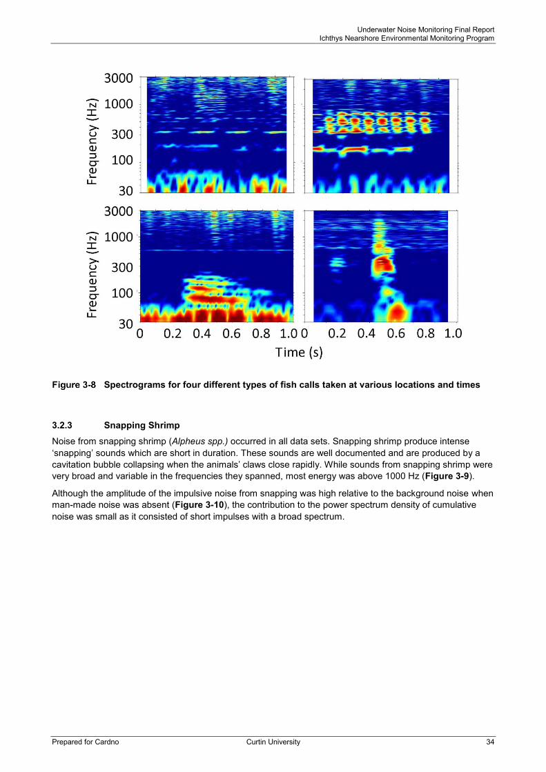
Underwater Noise Monitoring Final Report Ichthys Nearshore Environmental Monitoring Program
Prepared for Cardno Curtin University 34
Spectrograms for four different types of fish calls taken at various locations and times
3.2.3 Snapping Shrimp
Noise from snapping shrimp (Alpheus spp.) occurred in all data sets. Snapping shrimp produce intense ‘snapping’ sounds which are short in duration. These sounds are well documented and are produced by a cavitation bubble collapsing when the animals’ claws close rapidly. While sounds from snapping shrimp were very broad and variable in the frequencies they spanned, most energy was above 1000 Hz (Figure 3-9).
Although the amplitude of the impulsive noise from snapping was high relative to the background noise when man-made noise was absent (Figure 3-10), the contribution to the power spectrum density of cumulative noise was small as it consisted of short impulses with a broad spectrum.
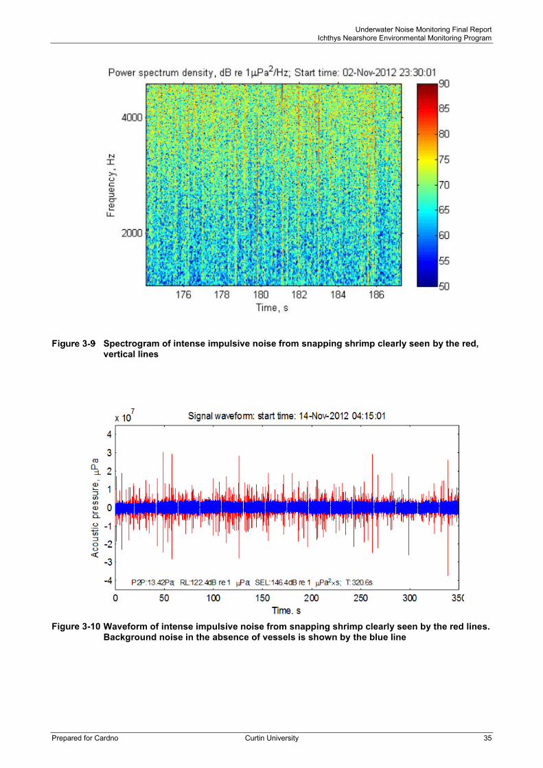
Underwater Noise Monitoring Final Report Ichthys Nearshore Environmental Monitoring Program
Prepared for Cardno Curtin University 35
Spectrogram of intense impulsive noise from snapping shrimp clearly seen by the red, vertical lines
Waveform of intense impulsive noise from snapping shrimp clearly seen by the red lines. Background noise in the absence of vessels is shown by the blue line

Underwater Noise Monitoring Final Report Ichthys Nearshore Environmental Monitoring Program
Prepared for Cardno Curtin University 36
3.3 Anthropogenic Noise During the recording period a range of sounds were recorded which were considered to be from anthropogenic sources. Anthropogenic sources included dredging, a range of vessel types using and transiting through Darwin Harbour, machinery being operated on the various vessels and dredgers, and pile driving. Noise from dredgers and vessels are described here. Noise from piling has been described in field reports on in situ measurements made as part of this underwater noise monitoring program (Gavrilov et al. 2015; Salgado Kent et al. 2014c; Gavrilov et al. 2012;) as well as in reports by other authors (INPEX 2014a).
3.3.1 Dredging
Cutter suction dredging and TSHDs in East Arm Darwin Harbour were carried out during two seasons: 4 November 2012 to 30 April 2013 (Season One) and 1 November 2013 to 11 June 2014 (Season Two; Table 2-1). The sediment composition differed significantly at the various dredging locations within the harbour monitored for underwater noise (INPEX 2012). Hard, fully or partly cemented sediment materials, such as conglomerate, sandstone and siltstone constitute more than 65% of bed material in the Walker Shoal area.
Example recordings were selected for detailed analyses of dredging noise when the CSD Athena was operating at Walker Shoal. INPEX provided the vessel positions and dredging status1 during: two days of operation of the CSD Athena (Figure 2-6) at Walker Shoal (Figure 2-7).
Table 3-6 Data subset extracted for detailed analyses of dredging noise Area CSD Athena
Walker Shoal (SP5) 2 days (10 and 11 Nov 2013)
In this section of the report, the characteristics of underwater noise created by the CSD operating at Walker Shoal is presented, followed by a comparison with the model predictions (URS 2011).
3.3.1.1 Noise Recorded during Operation for the CSD Athena at Walker Shoal
Underwater noise recorded between 12 am on 10 November and 12 am on 12 November 2013 were extracted from two noise loggers, one low-frequency (dataset 3236) and one high-frequency (dataset 3240HF), located in the downriver area of East Arm, approximately 650m from Walker Shoal (Figure 3-11). This noise corresponded with the period in which the CSD Athena was operating at Walker Shoal. The other pair of LF and HF noise loggers in East Arm (datasets 3238LF and 3239HF) was located further upriver near the berthing area, about 3 km away from the dredging site at Walker Shoal. Sea noise recordings made by these two more remote loggers did not reveal any trace of dredging noise from Walker Shoal. This is most likely due to the acoustic shadowing effect of South Shell Island in which underwater sound transmission was blocked between the dredging site and the noise loggers (see Figure 3-11). Both downriver loggers recorded dredging noise produced by the CSD Athena, with most of the dredging noise energy below 5 kHz, therefore data from the low-frequency logger (set 3236LF) were used for analysis.
1 defined as the removal of bottom material with the cutter/trailer head in direct contact with the seabed

Underwater Noise Monitoring Final Report Ichthys Nearshore Environmental Monitoring Program
Prepared for Cardno Curtin University 37
Locations of four sea noise loggers (red dots) deployed in East Arm of Darwin Harbour during the dredging operation in the Walker Shoal area. The area of dredging operation over the time period of dredging noise analysis is shown by the blue polygon
Periods of dredging noise are clearly visible in the long-time average spectrogram as long lasting intervals of intense broadband noise (Figure 3-12). The long-time average spectrogram and the sound pressure waveform from the individual 500-s noise recording (bottom panel of Figure 3-12) also show that the dredging noise level and spectrum varied considerably over time and as the dredger moved. The broadband Sound Pressure Level (SPL) sometimes rose as high as 150 dB re 1 μPa RMS.

Underwater Noise Monitoring Final Report Ichthys Nearshore Environmental Monitoring Program
Prepared for Cardno Curtin University 38
Long-time (500s) average spectrogram of underwater noise recorded by the LF logger near Walker Shoal from 9 to 12 November 2013 (top panel), and the sound pressure waveform of dredging noise from an individual 500-s recording (bottom panel)
Figure 3-13 demonstrates the correlation of the underwater noise level in a broad frequency band of 20 Hz to 1 kHz with the dredging activity. During dredging the underwater noise level in this frequency band was 10 dB to 30 dB higher than when the dredger was not operating. Statistics of the variation in the spectrum level of dredging noise in 1/3-octave frequency bands is illustrated by Figure 3-14. This figure shows the mean spectrum level of background noise in the absence of dredging (black dashed line) and percentiles of the spectrum levels measured for dredging noise. The Nth percentile shows the spectrum levels below which N% of all measurements of dredging noise fall in 1/3-octave bands. The 50th percentile gives the median values. This figure reveals that the maximum spectrum level of dredging noise at 500 Hz to 600 Hz stayed below 130 dB re 1 µPa2/Hz for about 99% of the time and exceeded 120 dB for approximately 50% of the time.

Underwater Noise Monitoring Final Report Ichthys Nearshore Environmental Monitoring Program
Prepared for Cardno Curtin University 39
Underwater noise level in a 20-1000 Hz frequency band (dashed line). The noise samples during the dredging operation of CSD Athena in the Walker Shoal area are indicated by red dots
Mean spectrum level of background underwater noise (dashed line) and percentiles of spectrum levels of dredging noise (colour lines) in 1/3-octave bands observed during the dredging operation of CSD Athena in the Walker Shoal area
3.3.1.4 Comparison to modelling predictions for the Walker Shoal area
SVT made predictions of underwater noise levels from dredging at Walker Shoal using the source spectrum level measured from a different type of CSD dredger and a numerical model of underwater sound propagation (URS 2011). The predictions of the broadband underwater noise levels from a CSD-type dredger operating over the southern edge of Walker Shoal are shown in Figure 3-15. According to these predictions, the broadband sound pressure level from the dredging operation would be approximately 125 dB re 1 µPa at 500 m and about 120 dB at 1 km from the dredger (Appendix A Table 5-3 in URS 2011). These
10/11/13 11/11/13 12/11/13110
115
120
125
130
135
140
145
150
155
Nois
e level (d
B r
e 1
P
a R
MS
)
Noise level in 20-1000 Hz frequency band
101
102
103
70
80
90
100
110
120
130
140
Frequency (Hz)
Pow
er
spectr
al density
(dB
re 1
P
a2
/ H
z)
1/3-octave dredging and background noise levels
dredging 99%
dredging 95%
dredging 75%
dredging 50%
dredging 25%
dredging 5%
mean background noise

Underwater Noise Monitoring Final Report Ichthys Nearshore Environmental Monitoring Program
Prepared for Cardno Curtin University 40
levels are more than 20 dB lower than the approximate median broadband noise level of 145 dB (Figure 3-13) measured at distances from 630 m to 680 m from the dredger at the Walker Shoal site on 10 and 11 November 2013.
Contours of received broadband sound pressure levels of underwater noise from a CSD dredger operating in the southern part of Walker Shoal (URS 2011)
3.3.2 Vessels
Noise from vessels was highly variable in frequency and intensity. While the type of vessel, speed, type of machinery on the vessel and the distance from the noise logger were not recorded during this program, underwater noise characteristics of vessels are known to be directly related to these attributes. The most intense noise from a vessel is generally from propeller cavitation for vessels that use propellers for propulsion. Bubbles are created when there is sufficient low pressure areas created by rotating propeller blades. The bubbles grow, collapse and rebound. This oscillation of bubbles creates intense noise. For vessels having machinery, machinery noise transmits into the water through the hull of vessels. Machinery can include engines, pumps, and generators, among other sources which create a range of sounds.
Underwater noise from vessels recorded during the monitoring program was always broadband, with most energy ranging from tens of Hz to several kHz (Figure 3-16, Figure 3-17 and Figure 3-18) with a peak in energy often occurring between 20 and 200 Hz. The example of vessel noise in Figure 3-16 shows the broadband noise energy as well as tonal components mainly below 70 Hz mainly resulting from the blade rotation rate. Vessels passing by an acoustic receiver have ‘V’ shaped patterns in the energy of the power spectrum (see Figure 3-16). This is a result of the noise transmission paths from the source located close to the sea surface. The ‘V’ shaped pattern is not as evident for a slowly moving vessel (Figure 3-17).

Underwater Noise Monitoring Final Report Ichthys Nearshore Environmental Monitoring Program
Prepared for Cardno Curtin University 41
Spectrogram showing intense noise from a vessel passing nearby
Waveform (left panel) and spectrogram (right panel) of intense broadband noise from a slowly moving vessel with the maximum received signal level of 149 dB re 1Pa
While noise from vessels could be relatively intense with noise levels often above 130 and 140 dB re 1Pa (Figure 3-17), occasionally energy from vessels was superimposed upon energy from dredging and could not be separated (Figure 3-18).

Underwater Noise Monitoring Final Report Ichthys Nearshore Environmental Monitoring Program
Prepared for Cardno Curtin University 42
Example of broadband transport vessel superimposed on background dredging noise measured at a range of ~360 m.
Overall, the frequent occurrence of relatively intense, transient broadband noise reflected the Port’s use by large vessels and cargo ships often operating under load. Smaller vessels were also frequently detected, identifiable by their relatively high frequency ranges resulting from higher propeller blade rotation rates.
As an example, the spectrum level of noise recorded in the lower reaches of East Arm between 2 November 2012 and 14 December 2012 demonstrated major variations in the noise spectrum due to vessels and other anthropogenic noise. Noise levels exceeded 20 dB at frequencies between approximately 50 Hz and 1 kHz (Figure 3-19 and Figure 3-20). This frequency band contained most of the energy of man-made noise produced in the area during this period. The maximum contribution of man-made noise to the ambient noise environment was nearly 50 dB in this frequency band in this example.
Distance 1.0299 km
12 32' S
12 28' S
130 44' E 130
48' E 130
52' E 130
56' E
R25
0 50 100 150 200 250136
137
138
139
140
141
142
143
144
145
Time, s
Noi
se le
vel,
dB re
1 P
a
Noise from transport vessel at ~360m superimposed on dredging noise
Distance 1.0299 km
12 32' S
12 28' S
130 44' E 130
48' E 130
52' E 130
56' E
R25
Distance 1.0299 km
12 32' S
12 28' S
130 44' E 130
48' E 130
52' E 130
56' E
R25
0 50 100 150 200 250136
137
138
139
140
141
142
143
144
145
Time, s
Noi
se le
vel,
dB re
1 P
a
0 50 100 150 200 250136
137
138
139
140
141
142
143
144
145
Time, s
Noi
se le
vel,
dB re
1 P
a
Noise from transport vessel at ~360m superimposed on dredging noiseNoise from transport vessel at ~360m superimposed on dredging noise

Underwater Noise Monitoring Final Report Ichthys Nearshore Environmental Monitoring Program
Prepared for Cardno Curtin University 43
Mean power spectrum density (PSD) of underwater noise measured by the LF logger between 2 November 2012 and 14 December 2012 in 1/3-octave frequency bands (±standard deviation)
Power spectrum density (PSD) of underwater noise with median, minimum and maximum levels in 1/3-octave frequency bands measured by the LF logger between 2 November 2012 and 14 December 2012
10 100 100050
60
70
80
90
100
110
Frequency (Hz)
PS
D (d
B re
1
Pa2
/ Hz)
10 100 100050
60
70
80
90
100
110
Frequency (Hz)
PS
D (d
B re
1
Pa2
/ Hz)
10 100 100040
50
60
70
80
90
100
110
120
130
Frequency (Hz)
PSD
(dB
re 1
Pa
2/ H
z)
medianminimummaximum
10 100 100040
50
60
70
80
90
100
110
120
130
Frequency (Hz)
PSD
(dB
re 1
Pa
2/ H
z)
medianminimummaximum
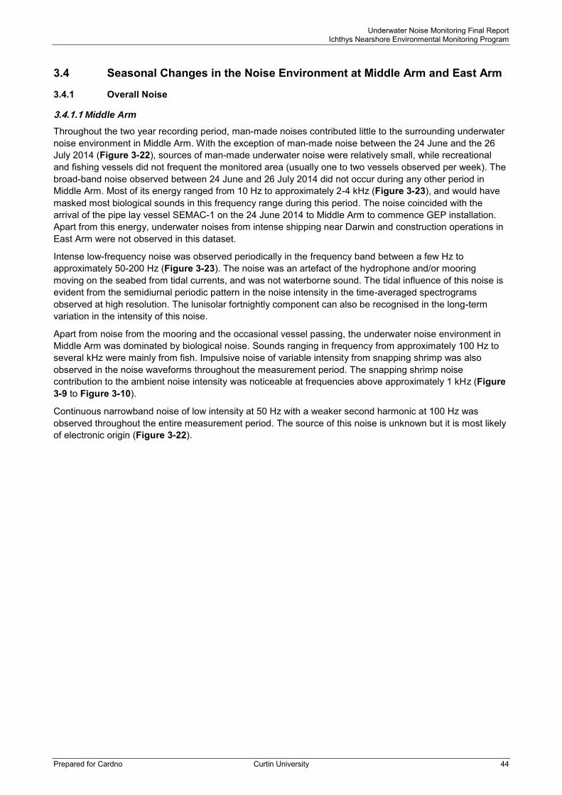
Underwater Noise Monitoring Final Report Ichthys Nearshore Environmental Monitoring Program
Prepared for Cardno Curtin University 44
3.4 Seasonal Changes in the Noise Environment at Middle Arm and East Arm
3.4.1 Overall Noise
3.4.1.1 Middle Arm
Throughout the two year recording period, man-made noises contributed little to the surrounding underwater noise environment in Middle Arm. With the exception of man-made noise between the 24 June and the 26 July 2014 (Figure 3-22), sources of man-made underwater noise were relatively small, while recreational and fishing vessels did not frequent the monitored area (usually one to two vessels observed per week). The broad-band noise observed between 24 June and 26 July 2014 did not occur during any other period in Middle Arm. Most of its energy ranged from 10 Hz to approximately 2-4 kHz (Figure 3-23), and would have masked most biological sounds in this frequency range during this period. The noise coincided with the arrival of the pipe lay vessel SEMAC-1 on the 24 June 2014 to Middle Arm to commence GEP installation. Apart from this energy, underwater noises from intense shipping near Darwin and construction operations in East Arm were not observed in this dataset.
Intense low-frequency noise was observed periodically in the frequency band between a few Hz to approximately 50-200 Hz (Figure 3-23). The noise was an artefact of the hydrophone and/or mooring moving on the seabed from tidal currents, and was not waterborne sound. The tidal influence of this noise is evident from the semidiurnal periodic pattern in the noise intensity in the time-averaged spectrograms observed at high resolution. The lunisolar fortnightly component can also be recognised in the long-term variation in the intensity of this noise.
Apart from noise from the mooring and the occasional vessel passing, the underwater noise environment in Middle Arm was dominated by biological noise. Sounds ranging in frequency from approximately 100 Hz to several kHz were mainly from fish. Impulsive noise of variable intensity from snapping shrimp was also observed in the noise waveforms throughout the measurement period. The snapping shrimp noise contribution to the ambient noise intensity was noticeable at frequencies above approximately 1 kHz (Figure 3-9 to Figure 3-10).
Continuous narrowband noise of low intensity at 50 Hz with a weaker second harmonic at 100 Hz was observed throughout the entire measurement period. The source of this noise is unknown but it is most likely of electronic origin (Figure 3-22).

Underwater Noise Monitoring Final Report Ichthys Nearshore Environmental Monitoring Program
Prepared for Cardno Curtin University 45
Spectrograms of sea noise recorded in Middle Arm using Low Frequency noise loggers over the first 18 months of the underwater noise measurement program
Noise from movement of the mooring
Energy from fish choruses
Energy from snapping shrimp
2012 2013
2014

Underwater Noise Monitoring Final Report Ichthys Nearshore Environmental Monitoring Program
Prepared for Cardno Curtin University 46
Spectrograms of sea noise recorded in Middle Arm using Low Frequency noise loggers over the last eight months of the underwater noise measurement program
Waveform (left panel) and spectrogram (right panel) at high time resolution of man-made noise recorded at 20:00 on the 24 June 2014 on LF 3322
Man-made noise atypical of Middle Arm
Possible electronic noise at 50 Hz
2014 2015

Underwater Noise Monitoring Final Report Ichthys Nearshore Environmental Monitoring Program
Prepared for Cardno Curtin University 47
3.4.1.2 Lower East Arm
The underwater noise environment in the lower reaches of East Arm near the entrance of the Port, was dominated by shipping noise and other man-made sources of underwater noise associated with operations requiring movement of equipment or vessels in and out of the port (e.g. machinery noise). Often it was not possible to identify individual noise sources in such a complex noise environment. Man-made noise was most intense between the 23 April and the 30 April 2013, and was due to dredging within proximity of the noise logger (Figure 3-24 and Figure 3-25). Intense broadband man-made noise from vessels and machinery also occurred typically between 5 to 20 times per day throughout the recording period in the frequency band of approximately 10 Hz to 2 kHz. Periods of intense man-made broadband noise, lasting from approximately 1 hour to 5 hours also were observed over the recording period. The frequency band of this noise was from approximately 5 Hz to nearly 2 kHz. Because the spectrum was broad and relatively flat it was most likely from cavitation noise from a large propeller or perhaps a pump impeller, rather than machinery noise. The intensity level of this noise ranged from below 110 dB re 1 µPa to above 130 dB re 1 µPa during some periods.
Noises of biological origin such as fish were observed when man-made noise was not present, although these were not as detectable as in Middle Arm and often masked behind man-made noise. Snapping shrimp were also present throughout this dataset.
As in the recording in Middle Arm, low-frequency noise ranging from 5 Hz to approximately 200 Hz was present throughout the recordings, which appear characteristic of movement of the mooring or hydrophone, or material against the hydrophone during tidal flows.

Underwater Noise Monitoring Final Report Ichthys Nearshore Environmental Monitoring Program
Prepared for Cardno Curtin University 48
Spectrograms of sea noise recorded over the two year period in Lower East Arm with Low Frequency noise loggers
Shipping and vessel noise Intense man-made
noise
2014
2012 2013
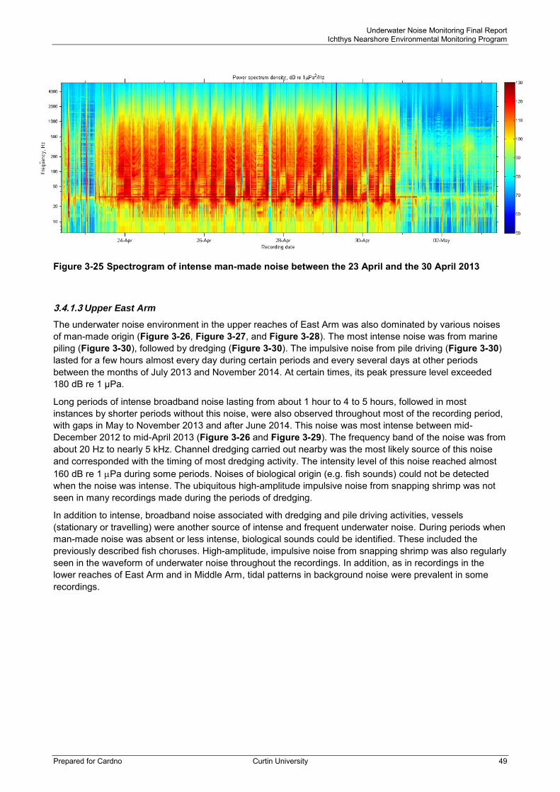
Underwater Noise Monitoring Final Report Ichthys Nearshore Environmental Monitoring Program
Prepared for Cardno Curtin University 49
Spectrogram of intense man-made noise between the 23 April and the 30 April 2013
3.4.1.3 Upper East Arm
The underwater noise environment in the upper reaches of East Arm was also dominated by various noises of man-made origin (Figure 3-26, Figure 3-27, and Figure 3-28). The most intense noise was from marine piling (Figure 3-30), followed by dredging (Figure 3-30). The impulsive noise from pile driving (Figure 3-30) lasted for a few hours almost every day during certain periods and every several days at other periods between the months of July 2013 and November 2014. At certain times, its peak pressure level exceeded 180 dB re 1 µPa.
Long periods of intense broadband noise lasting from about 1 hour to 4 to 5 hours, followed in most instances by shorter periods without this noise, were also observed throughout most of the recording period, with gaps in May to November 2013 and after June 2014. This noise was most intense between mid-December 2012 to mid-April 2013 (Figure 3-26 and Figure 3-29). The frequency band of the noise was from about 20 Hz to nearly 5 kHz. Channel dredging carried out nearby was the most likely source of this noise and corresponded with the timing of most dredging activity. The intensity level of this noise reached almost 160 dB re 1 Pa during some periods. Noises of biological origin (e.g. fish sounds) could not be detected when the noise was intense. The ubiquitous high-amplitude impulsive noise from snapping shrimp was not seen in many recordings made during the periods of dredging.
In addition to intense, broadband noise associated with dredging and pile driving activities, vessels (stationary or travelling) were another source of intense and frequent underwater noise. During periods when man-made noise was absent or less intense, biological sounds could be identified. These included the previously described fish choruses. High-amplitude, impulsive noise from snapping shrimp was also regularly seen in the waveform of underwater noise throughout the recordings. In addition, as in recordings in the lower reaches of East Arm and in Middle Arm, tidal patterns in background noise were prevalent in some recordings.

Underwater Noise Monitoring Final Report Ichthys Nearshore Environmental Monitoring Program
Prepared for Cardno Curtin University 50
Spectrograms of sea noise recorded over the two year period in Upper East Arm over the first 15 months of the underwater noise measurement program (note: scale of the bottom, left spectrogram differs from scales of other spectrograms due to a variation in logger settings).
Dredging noise
Dredging and pile driving noise
2014
2013
Low signal due to faulty
connection

Underwater Noise Monitoring Final Report Ichthys Nearshore Environmental Monitoring Program
Prepared for Cardno Curtin University 51
Spectrograms of sea noise recorded in Upper East Arm over the 16th to the 18th month (Aug-Nov 2014) of the underwater noise measurement program
Artefacts possibly from electronic noise
2014

Underwater Noise Monitoring Final Report Ichthys Nearshore Environmental Monitoring Program
Prepared for Cardno Curtin University 52
Spectrograms of sea noise recorded in Upper East Arm over the last 3 months of the underwater noise measurement program
2015 2014

Underwater Noise Monitoring Final Report Ichthys Nearshore Environmental Monitoring Program
Prepared for Cardno Curtin University 53
High frequency (top panel) and low frequency (middle panel) long-term average spectrograms of sea noise recorded on an HF logger over a 10-day period between 15 December and 25 December 2012. The bottom panels show the waveform (left) and spectrogram (right) of continuous broadband noise, likely from dredging

Underwater Noise Monitoring Final Report Ichthys Nearshore Environmental Monitoring Program
Prepared for Cardno Curtin University 54
Pile driving (upper panels) and dredging noise (lower panels) waveforms (left panels) and spectrograms (right panels) from recordings on the 16 and 17 May 2014

Underwater Noise Monitoring Final Report Ichthys Nearshore Environmental Monitoring Program
Prepared for Cardno Curtin University 55
3.4.1.1 Underwater noise levels in association with construction activities
Underwater noise was recorded over approximately 26 months from November 2012 to January 2015. Dredging and/or pile driving was undertaken intermittently during 23 months, 6 months of which was dredging only, 9 months of which was only pile driving, and 8 months of which was both dredging and pile driving. Neither dredging nor pile driving occurred between May and June 2013 and after November 2015.
The underwater noise levels recorded during this program had greater variability in East Arm than in Middle Arm, with high levels generally coinciding with dredging and pile driving. On average, underwater noise levels were 5 to 20 dB higher in East Arm than in Middle Arm. The high levels at the beginning of the deployment period in upper East Arm coincided with CSD dredging activity, and high levels from August 2013 to November 2014 coincided with pile driving and CSD and TSHD dredging. Noise levels dominated by anthropogenic sources measured in the lower and upper reaches of East Arm varied depending upon the distance between the logger and dredging and/or pile driving activities. Lower levels at all locations coincided with the cessation of Project construction activities between May and June 2013. However, even during periods without dredging and pile driving activities, average spectral levels were ~5-15 decibels greater in East Arm than in Middle Arm in some frequency bands due to more frequent and intense vessel noise in East Arm than in Middle Arm.

Underwater Noise Monitoring Final Report Ichthys Nearshore Environmental Monitoring Program
Prepared for Cardno Curtin University 56
3.4.2 Dolphins
Dolphin echolocation click trains were detected on six occasions, while whistles were detected on only one occasion. All detections occurred between May 2013 and August 2013 in East Arm (Figure 3-31). Such few acoustic dolphin detections were either due to dolphins not spending much time within the vicinity of the sea noise loggers, or dolphins not producing sound when within the detection range of the noise loggers.
Underwater recording data subsets reviewed for dolphin detections over the monitoring period, with dolphin detections indicated with a red cross. Balls with connecting lines of different colours depict independent deployment periods (lasting approximately 2 to 3 months each)
3.4.3 Fish
Presence by site of each chorus across the entire recording period can be seen in Figure 3-32 to Figure 3-40, broadly illustrating some interesting patterns in calling.
Chorus I (Terapontidae, grunters) displayed a clear semi-lunar pattern commencing on, or shortly after, the new and full moons, each month. The chorus lasted for several days depending on the time of year. The chorus was least present and weakest during the early period of the dry season (May to September), increasing in the lead up to the wet season and then displaying the highest levels, for the longest periods during the wet season. The timing and presence of the chorus was similar in 2014-2015 wet season, post construction, to the 2012-2013 wet season, pre-construction activity. While received levels due to the chorus could not always be determined due to masking by ambient noise the chorus could, on many occasions, be

Underwater Noise Monitoring Final Report Ichthys Nearshore Environmental Monitoring Program
Prepared for Cardno Curtin University 57
detected. The commencement and number of days the chorus was present did not vary considerably between new and full moons, however, the difference between wet and dry season was marked. Although there were few data points, the difference in the number of days in each season for 2013, compared with 2014 was minimal at Middle Arm, though there was a small difference in the East Arm Sites in the dry season.
Chorus II (Black jewfish, Protonibea diacanthus) was only present on a few occasions, at the Middle Arm site, and almost all, during the height of the wet season, between mid-November and mid-March. Each time this chorus also appeared within a few days of the new or full moon, lasting only for a few days, up to a maximum of a week (Table 3-7). Low levels of the chorus were also detected for a few days in May 2013 at the Middle Arm site and also the Lower East Arm site.
Chorus III (Batfish, Zabidius novemaculeatus) was predominantly present towards the end of the wet season through to the end of the dry season (Figure 3-34). However, while it was regularly present at Sites 1 and 2 in May and June 2013, it was only present at Site 1 for six days around the start of June in 2014. August for both years was the most prolonged period for the chorus, across all three sites; however, in 2014, it was only detected for approximately 55% of the total time of the previous year (63%, 46% and 55% for the Middle Arm, Lower East and Upper East Arms respectively).
Chorus IV, present predominantly in the lower reaches of the Middle and East Arms was only observed during the dry season. Visual scrutiny of the spectrograms would suggest that chorus levels were highest after the new and full moons, though there is insufficient data to test this. The chorus was present at similar periods during the 2013 and 2014 dry seasons.
Chorus V was present between February and October in 2013 and 2014, but absent during the height of the wet season. Received levels due to this chorus were not particularly high and of several thin frequency bands. As a result, increased ambient noise often masked the chorus and the peak calling during the season could not be ascertained.
Chorus VI was only observed at the Upper East Arm site, during the 2013 dry season and appeared to peak around the new moon. It was conspicuous in its absence from the same site in the 2014 dry season, however, with limited information on the source species and chorus data from previous years it is difficult to determine the reasons for the variation in this chorus.
Chorus VII produced low received levels and occurred at times and frequencies overlapping that of Choruses I and II. As a result, it is likely that this chorus often went undetected, providing limited data. The limited number of detections occurred predominantly 1 to 5 days after the new or full moons (Table 3-7).
Chorus VIII was also a comparatively low level chorus, comprising fewer callers than Choruses I-VII. It was predominantly present during the dry seasons, between the end of March and October, but also appeared in a weaker form at the Middle Arm and Lower East Arm sites in January 2013, 2014 and 2015. The chorus’ levels varied significantly across all recordings and with significant masking occurring it is not possible to determine when the peaks occurred.
Chorus IX produced particularly low received levels and could therefore be masked at any time. The few detections of this chorus were not sufficient to infer any lunar or seasonal patterns.

Underwater Noise Monitoring Final Report Ichthys Nearshore Environmental Monitoring Program
Prepared for Cardno Curtin University 58
Presence and qualitative split of relative intensity of Chorus I for the Middle Arm, Lower East Arm and Upper East Arm (Sites 1,2 and 3 respectively – Site 4 provided an alternate Upper Middle Arm recording for the first two months only) across all recording periods
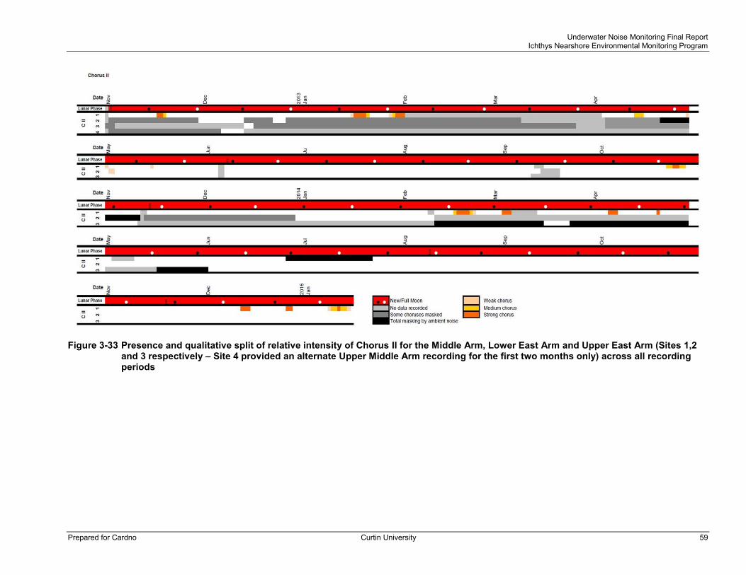
Underwater Noise Monitoring Final Report Ichthys Nearshore Environmental Monitoring Program
Prepared for Cardno Curtin University 59
Presence and qualitative split of relative intensity of Chorus II for the Middle Arm, Lower East Arm and Upper East Arm (Sites 1,2 and 3 respectively – Site 4 provided an alternate Upper Middle Arm recording for the first two months only) across all recording periods

Underwater Noise Monitoring Final Report Ichthys Nearshore Environmental Monitoring Program
Prepared for Cardno Curtin University 60
Presence and qualitative split of relative intensity of Chorus III for the Middle Arm, Lower East Arm and Upper East Arm (Sites 1,2 and 3 respectively) across all recording periods

Underwater Noise Monitoring Final Report Ichthys Nearshore Environmental Monitoring Program
Prepared for Cardno Curtin University 61
Presence and qualitative split of relative intensity of Chorus IV for the Middle Arm, Lower East Arm and Upper East Arm (Sites 1,2 and 3 respectively) across all recording periods
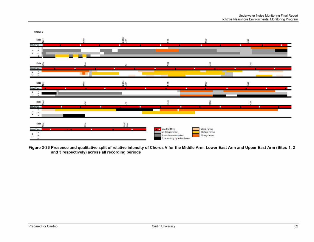
Underwater Noise Monitoring Final Report Ichthys Nearshore Environmental Monitoring Program
Prepared for Cardno Curtin University 62
Presence and qualitative split of relative intensity of Chorus V for the Middle Arm, Lower East Arm and Upper East Arm (Sites 1, 2 and 3 respectively) across all recording periods
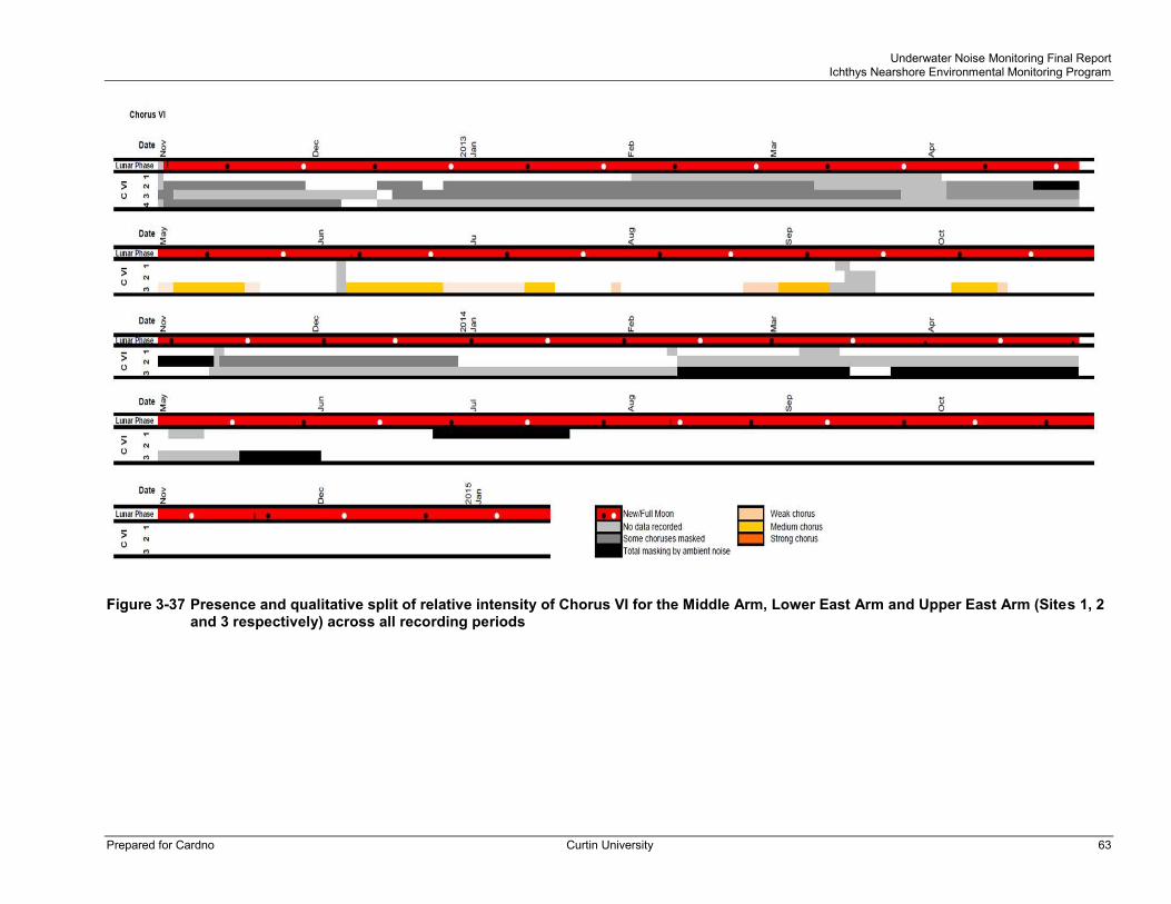
Underwater Noise Monitoring Final Report Ichthys Nearshore Environmental Monitoring Program
Prepared for Cardno Curtin University 63
Presence and qualitative split of relative intensity of Chorus VI for the Middle Arm, Lower East Arm and Upper East Arm (Sites 1, 2 and 3 respectively) across all recording periods

Underwater Noise Monitoring Final Report Ichthys Nearshore Environmental Monitoring Program
Prepared for Cardno Curtin University 64
Presence and qualitative split of relative intensity of Chorus VII for the Middle Arm, Lower East Arm and Upper East Arm (Sites 1, 2 and 3 respectively) across all recording periods

Underwater Noise Monitoring Final Report Ichthys Nearshore Environmental Monitoring Program
Prepared for Cardno Curtin University 65
Presence and qualitative split of relative intensity of Chorus VIII for the Middle Arm, Lower East Arm and Upper East Arm (Sites 1, 2 and 3 respectively) across all recording periods

Underwater Noise Monitoring Final Report Ichthys Nearshore Environmental Monitoring Program
Prepared for Cardno Curtin University 66
Presence and qualitative split of relative intensity of Chorus IX for the Middle Arm, Lower East Arm and Upper East Arm (Sites 1, 2 and 3 respectively) across all recording periods

Underwater Noise Monitoring Final Report Ichthys Nearshore Environmental Monitoring Program
Prepared for Cardno Curtin University 67
Table 3-7 Number of days after new or full moon that the chorus commenced and the number of days it lasted at each site. Maximum, minimum and standard deviation are shown in parentheses
Middle Arm Lower East Arm Upper East Arm
Comparison No. chorus periods analysed
Sites 1, 2, 3 Days Post Moon No. days present Days Post Moon No. days present Days Post Moon No. days present
All chorus 46, 33, 26 1.9 (4, 0, 1.0) 6.6 (12, 2, 2.4) 2.8 (6, 1, 1.3) 5.5 (11, 1, 2.5) 3.2 (7, 0, 1.6) 4.3 (9, 1, 2.5)
All full moons 24, 18, 14 1.75 (4, 0, 1.22) 6.8 (11, 3, 2.4) 2.8 (5, 1, 1.2) 5.4 (9, 1, 2.5) 3.3 (6, 1, 1.3) 4 (9, 1, 2.6)
All new moons 22, 15, 11 2.0 (4, 1, 0.8) 6.3 (12, 2, 2.4) 2.7 (6, 1, 1.3) 5.6 (11, 1, 2.5) 3.2 (7, 0, 1.9) 4.6 (8, 1, 2.4)
All wet seasons 24, 18, 13 1.5 (3, 0, 1.0) 8.1 (12, 5, 1.9) 2.4 (5, 1, 1.2) 9.9 (11, 1, 2.2) 3.5 (7, 1, 1.6) 4.4 (9, 1, 3.0)
All dry seasons 22, 16, 13 2.3 (4, 1, 0.9) 4.9 (8, 2, 1.7) 3.1 (6, 1, 1.2) 3.8 (6, 1, 1.6) 2.9 (6, 0, 1.5) 4.2 (8, 2, 1.9)
2013 Wet season 6, 8, 5 1.4 (3, 0, 1.1) 7.75 (12, 6, 2.1) 2.3 (4, 1, 1.1) 6.9 (11, 1, 2.8) 4.2 (7, 2, 1.7) 2.5 (7, 1, 2.3)
2014 Wet season 11,3,1 1.2 (3, 0, 1.0) 8.4 (11, 5, 2.1) 4 (5, 3, 1) 6.3 (7, 6, 0.6) 4 2
2013 Dry season 12, 9, 8 2.7 (4, 1, 1.2) 4.75 (8, 2, 2.0) 3.9 (6, 3, 0.9) 2.8 (4, 1, 1.2) 2.5 (4, 0, 1.5) 4.75 (8, 2, 2.1)
2014 Dry season 11, 6, 5 1.9 (2, 1, 0.3) 5.1 (7, 3, 1.4) 2 (3, 1, 0.6) 5.3 (6, 5, 0.5) 3.6 (6, 3, 1.3) 3.2 (5, 2, 1.3)
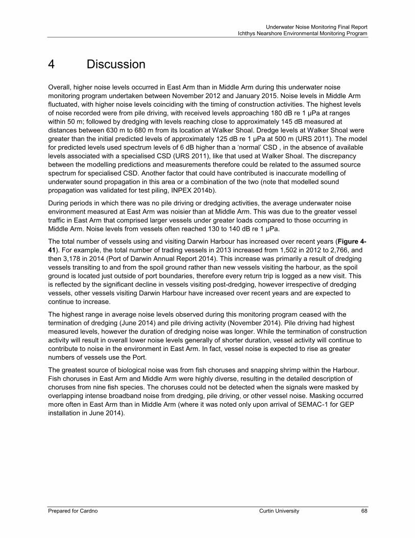
Underwater Noise Monitoring Final Report Ichthys Nearshore Environmental Monitoring Program
Prepared for Cardno Curtin University 68
4 Discussion
Overall, higher noise levels occurred in East Arm than in Middle Arm during this underwater noise monitoring program undertaken between November 2012 and January 2015. Noise levels in Middle Arm fluctuated, with higher noise levels coinciding with the timing of construction activities. The highest levels of noise recorded were from pile driving, with received levels approaching 180 dB re 1 µPa at ranges within 50 m; followed by dredging with levels reaching close to approximately 145 dB measured at distances between 630 m to 680 m from its location at Walker Shoal. Dredge levels at Walker Shoal were greater than the initial predicted levels of approximately 125 dB re 1 µPa at 500 m (URS 2011). The model for predicted levels used spectrum levels of 6 dB higher than a ‘normal’ CSD , in the absence of available levels associated with a specialised CSD (URS 2011), like that used at Walker Shoal. The discrepancy between the modelling predictions and measurements therefore could be related to the assumed source spectrum for specialised CSD. Another factor that could have contributed is inaccurate modelling of underwater sound propagation in this area or a combination of the two (note that modelled sound propagation was validated for test piling, INPEX 2014b).
During periods in which there was no pile driving or dredging activities, the average underwater noise environment measured at East Arm was noisier than at Middle Arm. This was due to the greater vessel traffic in East Arm that comprised larger vessels under greater loads compared to those occurring in Middle Arm. Noise levels from vessels often reached 130 to 140 dB re 1 µPa.
The total number of vessels using and visiting Darwin Harbour has increased over recent years (Figure 4-41). For example, the total number of trading vessels in 2013 increased from 1,502 in 2012 to 2,766, and then 3,178 in 2014 (Port of Darwin Annual Report 2014). This increase was primarily a result of dredging vessels transiting to and from the spoil ground rather than new vessels visiting the harbour, as the spoil ground is located just outside of port boundaries, therefore every return trip is logged as a new visit. This is reflected by the significant decline in vessels visiting post-dredging, however irrespective of dredging vessels, other vessels visiting Darwin Harbour have increased over recent years and are expected to continue to increase.
The highest range in average noise levels observed during this monitoring program ceased with the termination of dredging (June 2014) and pile driving activity (November 2014). Pile driving had highest measured levels, however the duration of dredging noise was longer. While the termination of construction activity will result in overall lower noise levels generally of shorter duration, vessel activity will continue to contribute to noise in the environment in East Arm. In fact, vessel noise is expected to rise as greater numbers of vessels use the Port.
The greatest source of biological noise was from fish choruses and snapping shrimp within the Harbour. Fish choruses in East Arm and Middle Arm were highly diverse, resulting in the detailed description of choruses from nine fish species. The choruses could not be detected when the signals were masked by overlapping intense broadband noise from dredging, pile driving, or other vessel noise. Masking occurred more often in East Arm than in Middle Arm (where it was noted only upon arrival of SEMAC-1 for GEP installation in June 2014).

Underwater Noise Monitoring Final Report Ichthys Nearshore Environmental Monitoring Program
Prepared for Cardno Curtin University 69
Trading vessels visiting Darwin Harbour in 2011/12, 2012/13, 2103/14 and 2014/15 (data from: Port of Darwin Trade Report 2015)

Underwater Noise Monitoring Final Report Ichthys Nearshore Environmental Monitoring Program
Prepared for Cardno Curtin University 70
The chorus described as ‘Chorus I’ was the most common chorus, present at all sites, across all seasons and years, and exhibited clearly defined patterns of calling. This chorus provided the best opportunity to consider variations in occurrence associated with anthropogenic noise. Chorus I displayed some variation between the dry season in 2013 and that of 2014, but these differences occurred to a varying extent at all three sites and were observed in a small number of samples. Thus little conclusion can be drawn on varying occurrence among sites. For Chorus I, one point of certainty is that that fish were calling within the vicinity regardless of anthropogenic noise (up to a level of masking at which a chorus could still be detected). This was also true for the other choruses described in this report although the lower received levels of the remaining choruses were likely to have been completely masked more often than Chorus I.
The continuation in calling behaviour in the presence of anthropogenic noise has been observed in other studies (Parsons et al. 2009) but does not imply that the fish are not affected by anthropogenic activity. If the calls are emitted for communication purposes in association with a behavioural function, such as to attract a mate during spawning, then while the emitter may continue their behaviour, the intended recipient may not detect the call. Any resulting impacts from the masking would be specific to the call function.
Dolphins, dugongs and turtles are species that use sound for reproduction, foraging, and in the case of dolphins for navigation. Hence these species were considered to be sensitive to potential impacts from man-made noise. Of these, this program aimed to detect sounds produced by dolphins. Dugongs produce sound comparatively infrequently and the overall low density of the animals was expected to reduce the probability of detection further. Dolphins, however, were detected on several occasions. Detection ranges were expected to be on the order of a few hundred meters to a maximum of a kilometre. All detections appeared to occur during a three month period between May 2013 and August 2013, and were mostly click trains used for echolocation. Echolocation click trains are used frequently during foraging, and repeated observations over several months often indicate a seasonal appearance of prey at a site. However, no further detections were made during the following year (2014) during the corresponding months. With few detections, it is not possible to associate the detections with changes in the natural environment or due to anthropogenic activity.
Underwater Noise Monitoring Final Report Ichthys Nearshore Environmental Monitoring Program
Prepared for Cardno Curtin University 71
5 Conclusion
In summary, dredging and pile driving in East Arm elevated background noise levels significantly in areas in proximity to construction activities; and Walker Shoal dredging noise levels were greater than modelled. In the absence of dredging and pile driving, the relatively high level of vessel traffic in East Arm contributed sufficient noise to produce a higher average noise level than in Middle Arm.
Despite the high human use in the north and north eastern areas of the harbour, there was a wide range and prevalence of fish choruses. As in this monitoring program, a continuation in calling behaviour by fish in the presence of anthropogenic noise has been observed in other studies. Dolphins, however, were detected infrequently during construction activities only, and were only detected in East Arm. Echolocation click trains are used regularly during foraging, and repeated observations over several months often indicate a seasonal appearance of prey at a site. While all detections were within the period of a few months, no further detections were made in the following year during the corresponding months. Dolphins were either mostly silent when travelling through the detection zone, spent minimal time within the detection zone, or both.

Underwater Noise Monitoring Final Report Ichthys Nearshore Environmental Monitoring Program
Prepared for Cardno Curtin University 72
5 References Au, W. W. L. (1993). The Sonar of Dolphins. New York: Springer-Verlag.
Chatto R. and Warneke R.M. (2000) Records of cetacean strandings in the Northern Territory of Australia. The Beagle, Records of the Museums and Art Galleries of the Northern Territory 16, 163-175.
Darwin Port Corporation (2015) Darwin Port Corporation 2015 Trade Report. http://www.darwinport.nt.gov.au/sites/default/files/images/DPC_2015_A-R_trade_report_web.pdf.
Department of Land Resource Management. 2015a. http://www.lrm.nt.gov.au/plants-and-animals/marine-and-coastal-biodiversity/darwin-harbour#dolphin. Accessed 21 Oct 2015.
Department of Land Resource Management. 2015b. http://www.lrm.nt.gov.au/plants-and-animals/native-animals. Accessed 21 Oct 2015.
Dudzinski, K. M. (1996). Communication and behaviour in the Atlantic spotted dolphins (Stenella frontalis): Relationships between vocal and behavioural activities. Ph.D. Thesis, 133, 215.
Environment Protection and Biodiversity Conservation (EPBC) Act 1999.
Gavrilov, A., McCauley, R. and Salgado Kent, C. (2012) Measurements of underwater noise from dredging operation during East Arm Darwin Harbour development in December 2012 (Interim Report 1: In situ measurements). CMST Report 2013-3, Curtin University.
Gavrilov, A.G. and Parsons, M.J.G. (2014) A Matlab toolbox for the Characterisation Of Recorded Underwater Sound (CHORUS). Acoustics Australia, 42(3):191-196.
Gavrilov, A., Salgado Kent, C., and Pusey, G. (2015) Measurements of underwater noise from dredging operation during East Arm Darwin Harbour development in August 2014 (Report 10: In situ measurements). CMST Report 2014-51, Curtin University.
Gavrilov, A. and Salgado Kent, C. (2015) Measurements of underwater noise from dredging and port construction operations during East Arm Darwin Harbour development in August 2014 to November 2014 (Report 12: Stationary measurements). CMST Report 2015-9, Curtin University.
Gomelyuk, V.E. (2012) Assessment of Darwin Harbour fish communities using baited remote underwater video station (BRUVS). Report to Department of Land Resource Management, Darwin. 61 pp.
Hawkins, E. R. (2010). Geographic variations in the whistles of bottlenose dolphins (Tursiops aduncus) along the east and west coasts of Australia. Journal of the Acoustical Society of America, 128(2), 924-935.
Herzing, D. L. (1996). Vocalizations and associated underwater behaviour of free-ranging Atlantic spotted dolphins, Stenella frontalis and bottlenose dolphins, Tursiops truncatus. Aquatic Mammals, 22(2), 61-79.
Herzing, D. L. (2000). Acoustics and social behavior of wild dolphins: implications for a sound society. In W. W. L. Au, A. N. Popper & R. R. Fay (Eds.), Hearing by Whales and Dolphins. Springer Handbook of Auditory Research (pp. 225-272). New York: Springer Verlag.
Herzing, D. L. (2015). Synchronous and rhythmic vocalizations and correlated underwater behavior of free-ranging Atlantic spotted dolphins (Stenella frontalis) and bottlenose dolphins (Tursiops truncatus) in the Bahamas, Animal Behavior and Cognition. 2(1), 14-29.
INPEX (2010) Ichthys Gas Field Development Project: Draft Environmental Impact Statement. INPEX Operations Australia Pty Ltd.
INPEX (2011) Ichthys Gas Field Development Project: Supplement to the Draft Environmental Impact Statement. INPEX Operations Australia Pty Ltd.
INPEX (2012) Dredging and Spoil Disposal Management Plan – East Arm Rev 1. INPEX Operations Australia Pty Ltd.
INPEX (2013) Dredging and Spoil Disposal Management Plan – East Arm Rev 4. INPEX Operations Australia Pty Ltd.
INPEX (2014a) Dredging and Spoil Disposal Management Plan – Gas Export Pipeline Rev 6. INPEX Operations Australia Pty Ltd.
INPEX (2014b) Underwater Noise Management Plan Rev 3. INPEX Operations Australia Pty Ltd.
Luczkovich, J.J., Sprague, M.W., Johnson, S.E. and Pullinger, C. (1999). Delimiting spawning areas of weakfish Cynoscion regalis (family Sciaenidae) in Pamlico Sound, North Carolina using passive hydroacoustic surveys. Bioacoustics, 10:143-60.
Marley, S., Salgado Kent, C. McCauley, R. and Parsons, M. (2013). Measurements of underwater noise from dredging operation during East Arm Darwin Harbour development in April-June 2013 (Field Summary Report 4: Stationary measurements). CMST Report 2013-40, Curtin University.
May-Collado, L. J. (2013) Guyana dolphins (Sotalia guianensis) from Costa Rica emit whistles that vary with surface behaviors. Journal of the Acoustical Society of America. 134(4), EL359-EL365.
May-Collado, L. J., and Wartzok, D. (2008) A comparison of bottlenose dolphin whistles in the Atlantic Ocean: factors promoting whistle variation. Journal of Mammalogy. 89, 1229-1240.
McCauley, R.D. (2012). Fish choruses from the Kimberley, seasonal and lunar links as determined by long term sea noise monitoring, Proceedings of Acoustics 2012 - Fremantle, 21-23 November 2012, Fremantle, Australia
McCauley, R.D. (2001). Biological sea noise in northern Australia: Patterns of fish calling, PhD Thesis, James Cook University of North Queensland. 290 pp.
McCauley, R.D. & Cato, D.H. (2000). Patterns of fish calling in a nearshore environment in the Great Barrier Reef. The Royal Society, vol. 355, pp. 1289-93.

Underwater Noise Monitoring Final Report Ichthys Nearshore Environmental Monitoring Program
Prepared for Cardno Curtin University 73
McCauley, R., Gavrilov, A., Salgado Kent, C. (2013). Measurements of underwater noise from dredging operation during East Arm Darwin Harbour development in December 2012 to April 2013 (Interim Report 3: Stationary measurements). CMST Report 2013-27, Curtin University.
Mok, H.K., Yu, H.Y., Ueng, J.P. and We, R.C. (2009). Characterization of sounds of the blackspotted croaker Protonibea diacanthus (Sciaenidae) and localization of its spawning sites in estuarine coastal waters of Taiwan. Zoological Studies, 48(3): 325-333.
Mok, H.K., Parmentier, E., Chiu, K.H., Tsai, K.E., Chiu, P.H. and Fine, M.L. (2011). An Intermediate in the evolution of superfast sonic muscles, Frontiers in Zoology, 8:31-38
NT Heritage Conservation Act (1991).
Padovan, A.V. (1997). The water quality of Darwin Harbour: October 1990 – November 1991. Water Quality Branch, Water Resources Division, Department of Lands, Planning and Environment, NT Government, Report No. 34/1997D December 1997.
Parsons, M.J.G., McCauley, R.D., Mackie, M., Siwabessy, P.J., Duncan, A.J. (2009). Localisation of individual mulloway (Argyrosomus japonicus) within a spawning aggregation and their behaviour throughout a diel spawning period, ICES Journal of Marine Science, 66:1007-14.
Parsons, M.J.G., McCauley, R.D., Mackie, M. and Duncan, A.J. (2012). In situ source levels of mulloway (Argyrosomus japonicus) calls. Journal of the Acoustical Society of America, 132(5):3559-68.
Parsons, M.J.G., McCauley, R.D., and Mackie, M.C. (2013a). Characterisation of mulloway advertisement sounds. Acoustics Australia, 41(3): 196-201.
Parsons, M.J.G., Lewis, P., Longbottom, S.G., McCauley, R.D. and Fairclough, D. (2013b). Sound production by the West Australian dhufish (Glaucosoma hebraicum). Journal of the Acoustical Society of America, 134(4): 2701-2709.
Parsons, M.J.G., Longbottom, S.M., McCauley, R.D., and Fairclough, D.V. (2014). In situ calls of Western Australian dhufish (Glaucosoma hebraicum) Acoustics Australia, 42(1): 31-35.
Parsons, M., Salgado Kent, C. and McCauley, R. (2014). Measurements of underwater noise from dredging and port construction operations during East Arm Darwin Harbour development in May 2014 to August 2014 (Report 11: Stationary measurements). CMST Report 2014-54, Curtin University.
Salgado Kent, C., Gavrilov, A. and McCauley, R. (2013). Measurements of underwater noise from dredging operation during East Arm Darwin Harbour development in December 2012 (Interim Report 2: Stationary measurements). CMST Report 2013-9, Curtin University.
Salgado Kent, C. and McCauley, R. (2014). Measurements of underwater noise from dredging and port construction operations during East Arm Darwin Harbour development in November 2013 to February 2014 (Report 8: Stationary measurements). CMST Report 2014-21, Curtin University.
Salgado Kent, C. McCauley, R. and Gavrilov, A. (2014a). Measurements of underwater noise from dredging and port construction operation during East Arm Darwin Harbour development in June 2013 to September 2013 (Field Summary Report 5: Stationary measurements). CMST Report 2013-50, Curtin University.
Salgado Kent, C., Parsons, M., McCauley, R., Gavrilov A., and Lucke, K. (2014b). Measurements of underwater noise from dredging and port construction operation during East Arm Darwin Harbour development in September 2013 to November 2013 (Report 6: Stationary measurements). CMST Report 2014-5, Curtin University.
Salgado Kent, C., Gavrilov A., and McCauley, R. (2014c). Measurements of underwater noise from dredging operation during East Arm Darwin Harbour development in December (Report 7: In situ measurements). CMST Report 2014-20, Curtin University.
Salgado Kent, C., Parsons, M., Gavrilov A., and McCauley, R. (2015). Measurements of underwater noise from dredging and port construction operations during East Arm Darwin Harbour development in February 2014 to May 2014 (Report 9: Stationary measurements). CMST Report 2014-47, Curtin University.
Southall, B. L., et al. (2007). Marine mammal noise exposure criteria: initial scientific recommendations. Aquatic Mammals. 33(4), 411‐521.
SVT (2014). PLJ and MOF Piling Underwater Noise – 3rd Monitoring Campaign Month 3 Noise Logging Report. Report No. 1254080-22-100-Rev1.
Talbot, S. (2006). The water quality of Darwin Harbour: Decembeer 2002 – December 2004. Aims report no. 37. Australian Institute of Marine Science. 55 p.
Territory Parks and Wildlife Conservation Act (TPWC Act 2006).
URS (2009). Ichthys Gas Field Development Project: Review of Literature on Sound in the Ocean and on the Effects of Noise on Marine Fauna. Appendix 15 of the Draft EIS.INPEX Document No. C036-AH-REP-0020 Rev 2.
URS (2011). Ichthys Gas Field Development Project. Potential effects of underwater blasting, pile driving and dredging on sensitive marine fauna in Darwin Harbour. INPEX Document No. C036-AH-REP-0115.
Underwater Noise Monitoring Final Report Ichthys Nearshore Environmental Monitoring Program
Prepared for Cardno Curtin University 74
Appendix A: Reference Systems and Acoustic Units All locations use the WGS84 chart datum.
Underwater acoustic units can be confusing; therefore, a short description is given below. The units and their definitions used in this report are:
> Root-mean-square (RMS) pressure (Pa) and its level (or noise level, dB re 1Pa) – these measures are commonly used to characterise the acoustic intensity of continuous sea noise in a broad frequency band. The noise level is 10log(RMS pressure).
dB re 1Pa Broadband – this is the integrated energy across the full frequency bandwidth of the source. Usually, exact frequency bandwidths are not stated so it is assumed that the measurement encompasses the frequency range of dominant energy in the source (i.e. the signal energy outside this frequency range does not contribute to the overall source energy received).
dB re 1Pa across a 1/3 octave band – 1/3 octaves are recognised logarithmically increasing frequency bands used in airborne acoustic studies. Each band has a defined lower frequency, centre frequency and upper frequency. The dB re 1Pa within a 1/3 octave band is the intensity summed across the band. The 1/3 octave bands are normally referenced by their centre frequency. It transpires that most vertebrates hear frequencies in a similar fashion, thus 1/3 octave values are useful for studies of marine animal hearing.
> Power Spectrum Density (PSD, Pa2/Hz) and spectrum level (dB re 1Pa2/Hz) – these are characteristics of sea noise spectra. The power spectrum density characterise the noise power in each 1-Hz band of the spectrum. The spectrum level is 10log(PSD). These units are widely used in underwater acoustics and are useful for comparing the spectral components of different sources.
> Source Level (dB re 1Pa @ 1 m) – this is the intensity of a measured source at a reference range of 1 m, which has been assumed to be a point source and which has had the transmission loss correction for that range and frequency applied. The source level is then the intensity at 1-m range that the source would radiate if it were an infinitesimal point. Most real sources are not infinitesimal points so for large sources such as vessels and air gun arrays, where the radiated noise is actually the sum of many spatially separated sub-sources, source levels are never actually reached but are a theoretical construct. Source levels are useful for estimating the transmission of sources and comparing source total noise output.
APPENDIX A