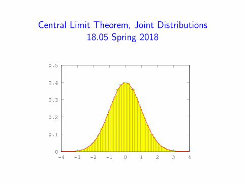
Central Limit Theorem, Joint Distributions18.05 Spring 2018

0

0.1

0.2

0.3

0.4

0.5

-4 -3 -2 -1 0 1 2 3 4

Exam next Wednesday

Exam 1 on Wednesday March 7, regular room and time.

Designed for 1 hour. You will have the full 80 minutes.

Class on Monday will be review.

Practice materials posted.

Learn to use the standard normal table for the exam.

No books or calculators.

You may have one 4× 6 notecard with any information you like.

February 27, 2018 2 / 31

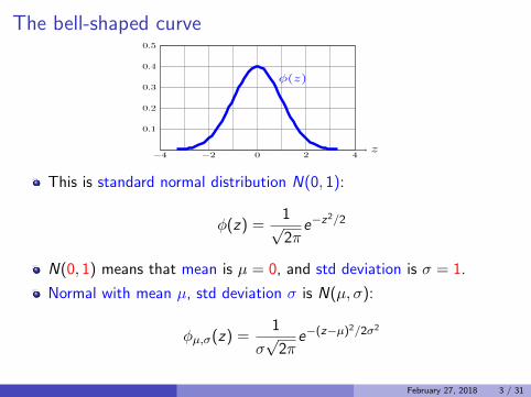
The bell-shaped curve

−4 −2 0 2 4

0.1

0.2

0.3

0.4

0.5

z

φ(z)

This is standard normal distribution N(0, 1):

φ(z) =1√2π

e−z2/2

N(0, 1) means that mean is µ = 0, and std deviation is σ = 1.

Normal with mean µ, std deviation σ is N(µ, σ):

φµ,σ(z) =1

σ√

2πe−(z−µ)

2/2σ2

February 27, 2018 3 / 31

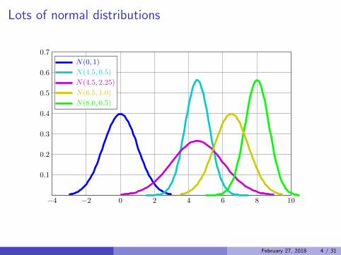
Lots of normal distributions

−4 −2 0 2 4 6 8 10

0.1

0.2

0.3

0.4

0.5

0.6

0.7

N(0, 1)

N(4.5, 0.5)

N(4.5, 2.25)

N(6.5, 1.0)

N(8.0, 0.5)

February 27, 2018 4 / 31

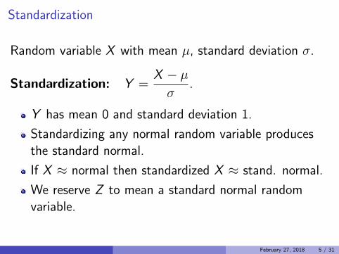
Standardization

Random variable X with mean µ, standard deviation σ.

Standardization: Y =X − µσ

.

Y has mean 0 and standard deviation 1.

Standardizing any normal random variable producesthe standard normal.

If X ≈ normal then standardized X ≈ stand. normal.

We reserve Z to mean a standard normal randomvariable.

February 27, 2018 5 / 31

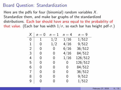
Board Question: Standardization

Here are the pdfs for four (binomial) random variables X .Standardize them, and make bar graphs of the standardizeddistributions. Each bar should have area equal to the probability ofthat value. (Each bar has width 1/σ, so each bar has height pdf·σ.)

X n = 0 n = 1 n = 4 n = 90 1 1/2 1/16 1/5121 0 1/2 4/16 9/5122 0 0 6/16 36/5123 0 0 4/16 84/5124 0 0 1/16 126/5125 0 0 0 126/5126 0 0 0 84/5127 0 0 0 36/5128 0 0 0 9/5129 0 0 0 1/512

February 27, 2018 6 / 31

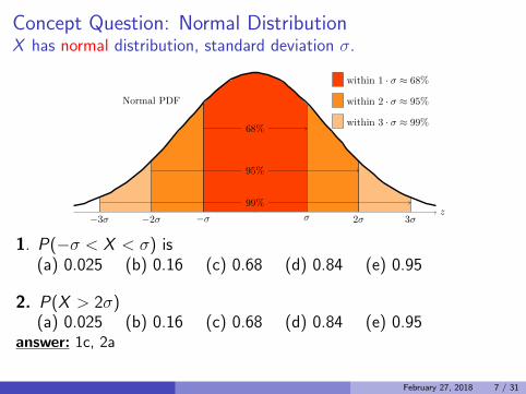
Concept Question: Normal DistributionX has normal distribution, standard deviation σ.

z−σ σ−2σ 2σ−3σ 3σ

Normal PDF

within 1 · σ ≈ 68%

within 2 · σ ≈ 95%

within 3 · σ ≈ 99%68%

95%

99%

1. P(−σ < X < σ) is(a) 0.025 (b) 0.16 (c) 0.68 (d) 0.84 (e) 0.95

2. P(X > 2σ)(a) 0.025 (b) 0.16 (c) 0.68 (d) 0.84 (e) 0.95

answer: 1c, 2a

February 27, 2018 7 / 31

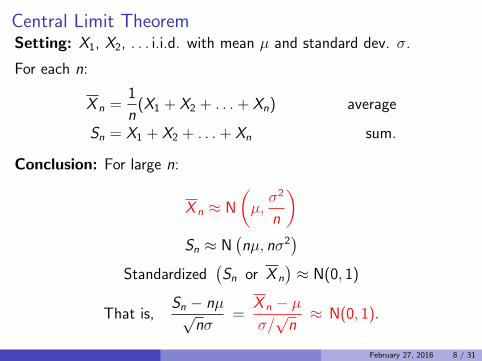
Central Limit TheoremSetting: X1, X2, . . . i.i.d. with mean µ and standard dev. σ.

For each n:

X n =1

n(X1 + X2 + . . . + Xn) average

Sn = X1 + X2 + . . . + Xn sum.

Conclusion: For large n:

X n ≈ N

(µ,σ2

n

)Sn ≈ N

(nµ, nσ2

)Standardized

(Sn or X n

)≈ N(0, 1)

That is,Sn − nµ√

nσ=

X n − µσ/√n≈ N(0, 1).

February 27, 2018 8 / 31

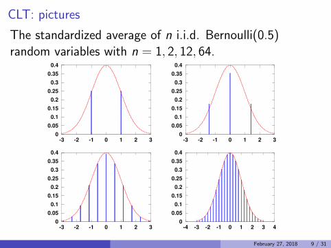
CLT: pictures

The standardized average of n i.i.d. Bernoulli(0.5)random variables with n = 1, 2, 12, 64.

0

0.05

0.1

0.15

0.2

0.25

0.3

0.35

0.4

-3 -2 -1 0 1 2 3

0

0.05

0.1

0.15

0.2

0.25

0.3

0.35

0.4

-3 -2 -1 0 1 2 3

0

0.05

0.1

0.15

0.2

0.25

0.3

0.35

0.4

-3 -2 -1 0 1 2 3

0

0.05

0.1

0.15

0.2

0.25

0.3

0.35

0.4

-4 -3 -2 -1 0 1 2 3 4

February 27, 2018 9 / 31

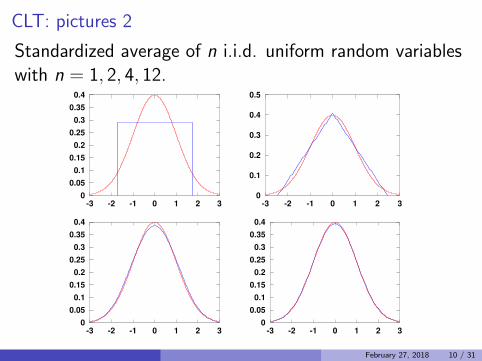
CLT: pictures 2

Standardized average of n i.i.d. uniform random variableswith n = 1, 2, 4, 12.

0

0.05

0.1

0.15

0.2

0.25

0.3

0.35

0.4

-3 -2 -1 0 1 2 3

0

0.1

0.2

0.3

0.4

0.5

-3 -2 -1 0 1 2 3

0

0.05

0.1

0.15

0.2

0.25

0.3

0.35

0.4

-3 -2 -1 0 1 2 3

0

0.05

0.1

0.15

0.2

0.25

0.3

0.35

0.4

-3 -2 -1 0 1 2 3

February 27, 2018 10 / 31

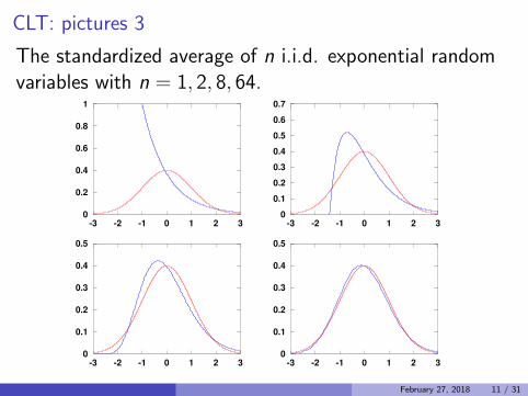
CLT: pictures 3

The standardized average of n i.i.d. exponential randomvariables with n = 1, 2, 8, 64.

0

0.2

0.4

0.6

0.8

1

-3 -2 -1 0 1 2 3

0

0.1

0.2

0.3

0.4

0.5

0.6

0.7

-3 -2 -1 0 1 2 3

0

0.1

0.2

0.3

0.4

0.5

-3 -2 -1 0 1 2 3

0

0.1

0.2

0.3

0.4

0.5

-3 -2 -1 0 1 2 3

February 27, 2018 11 / 31

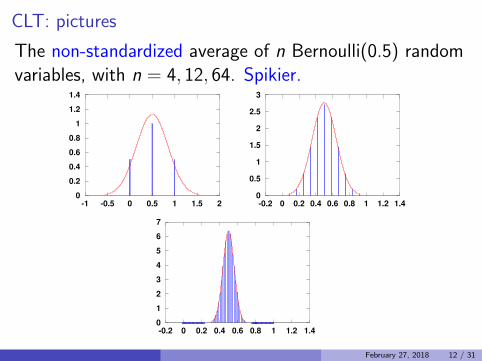
CLT: pictures

The non-standardized average of n Bernoulli(0.5) randomvariables, with n = 4, 12, 64. Spikier.

0

0.2

0.4

0.6

0.8

1

1.2

1.4

-1 -0.5 0 0.5 1 1.5 2

0

0.5

1

1.5

2

2.5

3

-0.2 0 0.2 0.4 0.6 0.8 1 1.2 1.4

0

1

2

3

4

5

6

7

-0.2 0 0.2 0.4 0.6 0.8 1 1.2 1.4

February 27, 2018 12 / 31

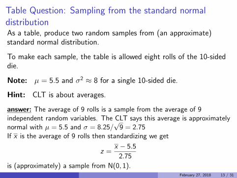
Table Question: Sampling from the standard normaldistributionAs a table, produce two random samples from (an approximate)standard normal distribution.

To make each sample, the table is allowed eight rolls of the 10-sideddie.

Note: µ = 5.5 and σ2 ≈ 8 for a single 10-sided die.

Hint: CLT is about averages.

answer: The average of 9 rolls is a sample from the average of 9independent random variables. The CLT says this average is approximatelynormal with µ = 5.5 and σ = 8.25/

√9 = 2.75

If x is the average of 9 rolls then standardizing we get

z =x − 5.5

2.75

is (approximately) a sample from N(0, 1).February 27, 2018 13 / 31

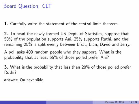
Board Question: CLT

1. Carefully write the statement of the central limit theorem.

2. To head the newly formed US Dept. of Statistics, suppose that50% of the population supports Ani, 25% supports Ruthi, and theremaining 25% is split evenly between Efrat, Elan, David and Jerry.

A poll asks 400 random people who they support. What is theprobability that at least 55% of those polled prefer Ani?

3. What is the probability that less than 20% of those polled preferRuthi?

answer: On next slide.

February 27, 2018 14 / 31

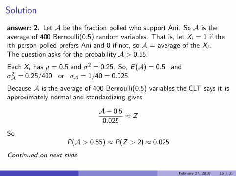
Solution

answer: 2. Let A be the fraction polled who support Ani. So A is theaverage of 400 Bernoulli(0.5) random variables. That is, let Xi = 1 if theith person polled prefers Ani and 0 if not, so A = average of the Xi .The question asks for the probability A > 0.55.

Each Xi has µ = 0.5 and σ2 = 0.25. So, E (A) = 0.5 andσ2A = 0.25/400 or σA = 1/40 = 0.025.

Because A is the average of 400 Bernoulli(0.5) variables the CLT says it isapproximately normal and standardizing gives

A− 0.5

0.025≈ Z

SoP(A > 0.55) ≈ P(Z > 2) ≈ 0.025

Continued on next slide

February 27, 2018 15 / 31

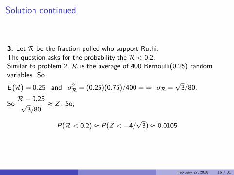
Solution continued

3. Let R be the fraction polled who support Ruthi.The question asks for the probability the R < 0.2.Similar to problem 2, R is the average of 400 Bernoulli(0.25) randomvariables. So

E (R) = 0.25 and σ2R = (0.25)(0.75)/400 =⇒ σR =√

3/80.

SoR− 0.25√

3/80≈ Z . So,

P(R < 0.2) ≈ P(Z < −4/√

3) ≈ 0.0105

February 27, 2018 16 / 31

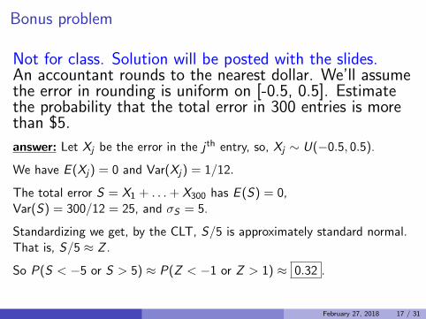
Bonus problem

Not for class. Solution will be posted with the slides.An accountant rounds to the nearest dollar. We’ll assumethe error in rounding is uniform on [-0.5, 0.5]. Estimatethe probability that the total error in 300 entries is morethan $5.

answer: Let Xj be the error in the j th entry, so, Xj ∼ U(−0.5, 0.5).

We have E (Xj) = 0 and Var(Xj) = 1/12.

The total error S = X1 + . . .+ X300 has E (S) = 0,Var(S) = 300/12 = 25, and σS = 5.

Standardizing we get, by the CLT, S/5 is approximately standard normal.That is, S/5 ≈ Z .

So P(S < −5 or S > 5) ≈ P(Z < −1 or Z > 1) ≈ 0.32 .

February 27, 2018 17 / 31

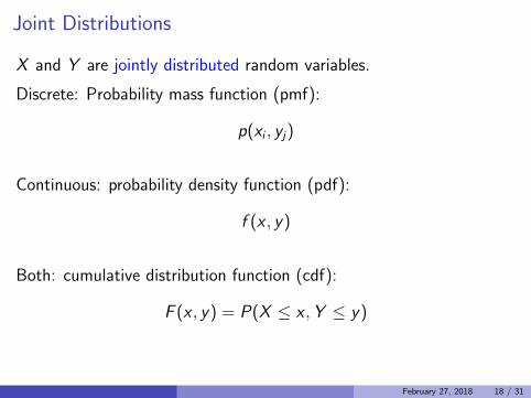
Joint Distributions

X and Y are jointly distributed random variables.

Discrete: Probability mass function (pmf):

p(xi , yj)

Continuous: probability density function (pdf):

f (x , y)

Both: cumulative distribution function (cdf):

F (x , y) = P(X ≤ x ,Y ≤ y)

February 27, 2018 18 / 31

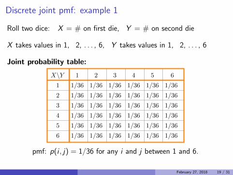
Discrete joint pmf: example 1

Roll two dice: X = # on first die, Y = # on second die

X takes values in 1, 2, . . . , 6, Y takes values in 1, 2, . . . , 6

Joint probability table:

X\Y 1 2 3 4 5 6

1 1/36 1/36 1/36 1/36 1/36 1/36

2 1/36 1/36 1/36 1/36 1/36 1/36

3 1/36 1/36 1/36 1/36 1/36 1/36

4 1/36 1/36 1/36 1/36 1/36 1/36

5 1/36 1/36 1/36 1/36 1/36 1/36

6 1/36 1/36 1/36 1/36 1/36 1/36

pmf: p(i , j) = 1/36 for any i and j between 1 and 6.

February 27, 2018 19 / 31

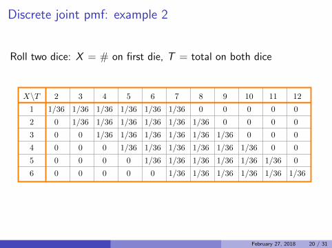
Discrete joint pmf: example 2

Roll two dice: X = # on first die, T = total on both dice

X\T 2 3 4 5 6 7 8 9 10 11 12

1 1/36 1/36 1/36 1/36 1/36 1/36 0 0 0 0 0

2 0 1/36 1/36 1/36 1/36 1/36 1/36 0 0 0 0

3 0 0 1/36 1/36 1/36 1/36 1/36 1/36 0 0 0

4 0 0 0 1/36 1/36 1/36 1/36 1/36 1/36 0 0

5 0 0 0 0 1/36 1/36 1/36 1/36 1/36 1/36 0

6 0 0 0 0 0 1/36 1/36 1/36 1/36 1/36 1/36

February 27, 2018 20 / 31

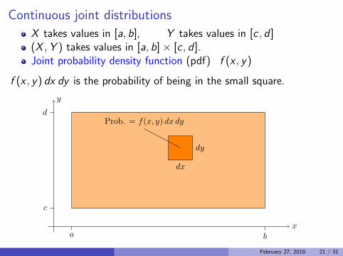
Continuous joint distributions

X takes values in [a, b], Y takes values in [c , d ](X ,Y ) takes values in [a, b]× [c , d ].Joint probability density function (pdf) f (x , y)

f (x , y) dx dy is the probability of being in the small square.

dx

dy

Prob. = f(x, y) dx dy

x

y

a b

c

d

February 27, 2018 21 / 31

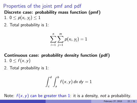
Properties of the joint pmf and pdfDiscrete case: probability mass function (pmf)1. 0 ≤ p(xi , yj) ≤ 1

2. Total probability is 1:

n∑i=1

m∑j=1

p(xi , yj) = 1

Continuous case: probability density function (pdf)1. 0 ≤ f (x , y)

2. Total probability is 1:∫ d

c

∫ b

a

f (x , y) dx dy = 1

Note: f (x , y) can be greater than 1: it is a density, not a probability.February 27, 2018 22 / 31

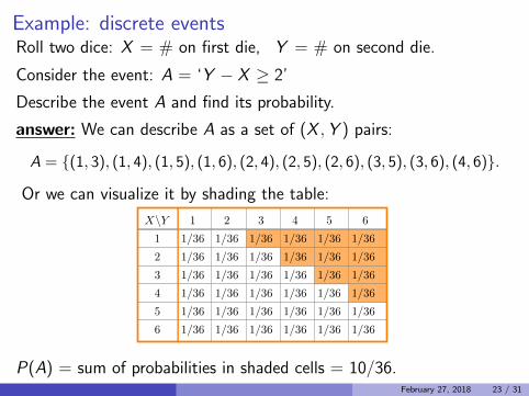
Example: discrete eventsRoll two dice: X = # on first die, Y = # on second die.

Consider the event: A = ‘Y − X ≥ 2’

Describe the event A and find its probability.

answer: We can describe A as a set of (X ,Y ) pairs:

A = {(1, 3), (1, 4), (1, 5), (1, 6), (2, 4), (2, 5), (2, 6), (3, 5), (3, 6), (4, 6)}.

Or we can visualize it by shading the table:

X\Y 1 2 3 4 5 6

1 1/36 1/36 1/36 1/36 1/36 1/36

2 1/36 1/36 1/36 1/36 1/36 1/36

3 1/36 1/36 1/36 1/36 1/36 1/36

4 1/36 1/36 1/36 1/36 1/36 1/36

5 1/36 1/36 1/36 1/36 1/36 1/36

6 1/36 1/36 1/36 1/36 1/36 1/36

P(A) = sum of probabilities in shaded cells = 10/36.February 27, 2018 23 / 31

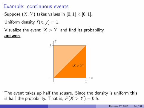
Example: continuous events

Suppose (X ,Y ) takes values in [0, 1]× [0, 1].

Uniform density f (x , y) = 1.

Visualize the event ‘X > Y ’ and find its probability.answer:

x

y

1

1

‘X > Y ’

The event takes up half the square. Since the density is uniform thisis half the probability. That is, P(X > Y ) = 0.5.

February 27, 2018 24 / 31

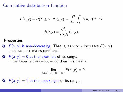
Cumulative distribution function

F (x , y) = P(X ≤ x , Y ≤ y) =

∫ y

c

∫ x

af (u, v) du dv .

f (x , y) =∂2F

∂x∂y(x , y).

Properties1. F (x , y) is non-decreasing. That is, as x or y increases F (x , y)

increases or remains constant.2. F (x , y) = 0 at the lower left of its range.

If the lower left is (−∞,−∞) then this means

lim(x ,y)→(−∞,−∞)

F (x , y) = 0.

3. F (x , y) = 1 at the upper right of its range.

February 27, 2018 25 / 31

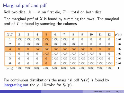
Marginal pmf and pdf

Roll two dice: X = # on first die, T = total on both dice.

The marginal pmf of X is found by summing the rows. The marginalpmf of T is found by summing the columns

X\T 2 3 4 5 6 7 8 9 10 11 12 p(xi)

1 1/36 1/36 1/36 1/36 1/36 1/36 0 0 0 0 0 1/6

2 0 1/36 1/36 1/36 1/36 1/36 1/36 0 0 0 0 1/6

3 0 0 1/36 1/36 1/36 1/36 1/36 1/36 0 0 0 1/6

4 0 0 0 1/36 1/36 1/36 1/36 1/36 1/36 0 0 1/6

5 0 0 0 0 1/36 1/36 1/36 1/36 1/36 1/36 0 1/6

6 0 0 0 0 0 1/36 1/36 1/36 1/36 1/36 1/36 1/6

p(tj) 1/36 2/36 3/36 4/36 5/36 6/36 5/36 4/36 3/36 2/36 1/36 1

For continuous distributions the marginal pdf fX (x) is found byintegrating out the y . Likewise for fY (y).

February 27, 2018 26 / 31

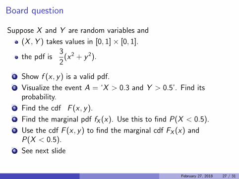
Board question

Suppose X and Y are random variables and

(X ,Y ) takes values in [0, 1]× [0, 1].

the pdf is3

2(x2 + y 2).

1 Show f (x , y) is a valid pdf.2 Visualize the event A = ‘X > 0.3 and Y > 0.5’. Find its

probability.3 Find the cdf F (x , y).4 Find the marginal pdf fX (x). Use this to find P(X < 0.5).5 Use the cdf F (x , y) to find the marginal cdf FX (x) and

P(X < 0.5).6 See next slide

February 27, 2018 27 / 31

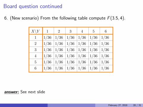
Board question continued

6. (New scenario) From the following table compute F (3.5, 4).

X\Y 1 2 3 4 5 6

1 1/36 1/36 1/36 1/36 1/36 1/36

2 1/36 1/36 1/36 1/36 1/36 1/36

3 1/36 1/36 1/36 1/36 1/36 1/36

4 1/36 1/36 1/36 1/36 1/36 1/36

5 1/36 1/36 1/36 1/36 1/36 1/36

6 1/36 1/36 1/36 1/36 1/36 1/36

answer: See next slide

February 27, 2018 28 / 31

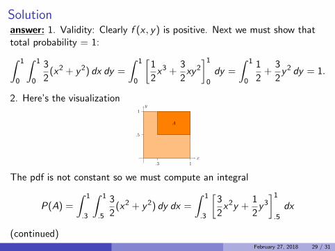
Solutionanswer: 1. Validity: Clearly f (x , y) is positive. Next we must show thattotal probability = 1:∫ 1

0

∫ 1

0

3

2(x2 + y2) dx dy =

∫ 1

0

[1

2x3 +

3

2xy2]10

dy =

∫ 1

0

1

2+

3

2y2 dy = 1.

2. Here’s the visualization

x

y

1.3

1

.5

A

The pdf is not constant so we must compute an integral

P(A) =

∫ 1

.3

∫ 1

.5

3

2(x2 + y2) dy dx =

∫ 1

.3

[3

2x2y +

1

2y3]1.5

dx

(continued)February 27, 2018 29 / 31

Solutions 2, 3, 4, 5

2. (continued) =

∫ 1

.3

3x2

4+

7

16dx = 0.5495

3. F (x , y) =

∫ y

0

∫ x

0

3

2(u2 + v2) du dv =

x3y

2+

xy3

2.

4.

fX (x) =

∫ 1

0

3

2(x2 + y2) dy =

[3

2x2y +

y3

2

]10

=3

2x2 +

1

2

P(X < .5) =

∫ .5

0fX (x) dx =

∫ .5

0

3

2x2 +

1

2dx =

[1

2x3 +

1

2x

].50

=5

16.

5. To find the marginal cdf FX (x) we simply take y to be the top of the

y -range and evalute F : FX (x) = F (x , 1) =1

2(x3 + x).

Therefore P(X < .5) = F (.5) =1

2(

1

8+

1

2) =

5

16.

6. On next slideFebruary 27, 2018 30 / 31

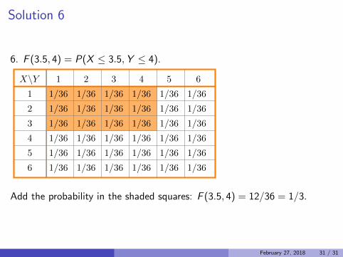
Solution 6

6. F (3.5, 4) = P(X ≤ 3.5,Y ≤ 4).

X\Y 1 2 3 4 5 6

1 1/36 1/36 1/36 1/36 1/36 1/36

2 1/36 1/36 1/36 1/36 1/36 1/36

3 1/36 1/36 1/36 1/36 1/36 1/36

4 1/36 1/36 1/36 1/36 1/36 1/36

5 1/36 1/36 1/36 1/36 1/36 1/36

6 1/36 1/36 1/36 1/36 1/36 1/36

Add the probability in the shaded squares: F (3.5, 4) = 12/36 = 1/3.

February 27, 2018 31 / 31