NBER WORKING PAPER SERIES

CENTRAL BANK SWAP ARRANGEMENTS IN THE COVID-19 CRISIS

Joshua AizenmanHiro Ito

Gurnain Kaur Pasricha

Working Paper 28585http://www.nber.org/papers/w28585

NATIONAL BUREAU OF ECONOMIC RESEARCH1050 Massachusetts Avenue

Cambridge, MA 02138March 2021, Revised August 2021

We would like to thank Apoorv Bhargava, Ricardo Cervantes, and Chau Nguyen for excellent research assistance. Insightful comments by Galina Hale and the participants of the JIMF SI “Financial Globalization and De- Globalization” conference, May 3-4, 2021 are gratefully acknowledged. We also appreciate the Latin American Reserve Fund (FLAR) for sharing with us the data on the currency shares in FX reserves for Latin American countries. We also thank Robert McCauley, Silvio Costa, Vassili Bazinas, Martin Kaufman, Gaston Gelos, Can Sever, Jeromin Zettelmeyer, participants at FLAR webinar in May 2021, and at two IMF seminars for useful comments and suggestions. The views expressed in the paper are those of the authors, and do not necessarily represent the views of the International Monetary Fund, its Executive Board or its management or the NBER.

NBER working papers are circulated for discussion and comment purposes. They have not been peer-reviewed or been subject to the review by the NBER Board of Directors that accompanies official NBER publications.

© 2021 by Joshua Aizenman, Hiro Ito, and Gurnain Kaur Pasricha. All rights reserved. Short sections of text, not to exceed two paragraphs, may be quoted without explicit permission provided that full credit, including © notice, is given to the source.

Central Bank Swap Arrangements in the COVID-19 Crisis Joshua Aizenman, Hiro Ito, and Gurnain Kaur Pasricha NBER Working Paper No. 28585March 2021, Revised August 2021JEL No. F15,F21,F32,F36,G15

ABSTRACT

Facing acute strains in the offshore dollar funding markets during the COVID-19 crisis, the Federal Reserve (Fed) implemented measures to provide US dollar liquidity through swap arrangements with other central banks and establishing a repo facility for financial institutions and monetary authorities (FIMA) in March 2020. This paper assesses motivations for the Fed liquidity lines, and the effects and spillovers of US dollar auctions by central banks. We find that the access to the liquidity arrangements was driven by the recipient economies’ close financial and trade ties with the US. Access to dollar liquidity also reflected global trade exposure. We find that announcements of expansion of Fed liquidity facilities or of auctions using these facilities led to appreciation of partner currencies against the US dollar. and reduced deviations from covered interest parity (CIP). Dollar auctions by major central banks (BoE, ECB, BoJ and SNB) led to temporary appreciation of other currencies against the US dollar, reduced CIP deviations, and persistently reduced sovereign bond yields of other economies. However, dollar auctions done by other central banks with access to Fed facilities did not have a meaningful impact on key domestic financial variables . The impact of major central bank auctions does not differ by the economies’ financial or trade links with the US or their balance sheet currency exposure, i.e. the major central bank auctions benefitted even the more vulnerable economies.

Joshua AizenmanEconomics and SIRUniversity of Southern CaliforniaUniversity ParkLos Angeles, CA 90089-0043and NBERaizenman@usc.edu

Hiro Ito15787 NW Hackney Dr.Portland, Oreg 97229USAito@pdx.edu

Gurnain Kaur PasrichaMonetary and Capital Markets DepartmentInternational Monetary Fund700 19th Street NW HQ1 6-590Washington, DC 20431gpasricha@imf.org

2

1. Introduction

The COVID-19 crisis saw an emergence of acute strains in the offshore dollar funding

markets in March 2020. As was the case during the Global Financial Crisis (GFC) of 2008, these

strains manifested as deviations from neo-classical arbitrage conditions, including deviations

from Covered Interest Parity (CIP) (Figure 1).1 Like in the last crisis, the US Federal Reserve

(Fed) took several actions to provide US dollar liquidity through foreign central banks. It

reduced the pricing of swap operations, extended the maturity, and increased the frequency of

swap operations with the five central banks with which it has standing swap lines. It also

reactivated swap lines with nine other central banks with which it had established the lines

during the GFC.

Furthermore, for the first time, on March 31, 2020, the Fed announced the establishment of

a temporary repurchase agreement facility for foreign and international monetary authorities

(FIMA). With this facility, the Fed allowed existing FIMA account holders at the New York

Federal Reserve to borrow dollars against US Treasuries they hold. The US dollars obtained by

the central banks can then be used for onward lending to institutions in their jurisdictions, thus

mitigating the US dollar liquidity shortage in these jurisdictions.

What motivates the Fed to extend dollar liquidity to selected foreign central banks?

Research on the extension of swap lines during the GFC suggests that US bank exposure to the

swap partner economies and the extent of reliance on the US as their export destination are

important motivations for the Fed to extend these lines (Aizenman and Pasricha, 2010;

Aizenman, Jinjarak, and Park, 2011).

Given that the economic environment in the COVID turmoil was different from that of the

GFC (which was driven by a shock that originated in the US financial system) and that FIMA

facility was added as another liquidity provision scheme, one may ask whether the factors

motivating the US decision to provide dollar liquidity were different in this crisis. Did the Fed

extend swap lines or develop the FIMA facility solely based on its self-interest as it did during

the GFC? What factors determined economies’ access to dollar liquidity? One may also ask to

1 See Du et al. (2018), and Liao and Zhang (2020) for linking these deviations to countries’ net foreign asset positions and the hedging channel of exchange rate determination.

3

what extent the size of US dollar auctions conducted by central banks reflected stress in domestic

financial or currency markets.

The economic impacts of these liquidity facilities are also worth investigating. Were they

effective in mitigating financial stress, and if so, which facilities? The announcements of swap

lines during the GFC had relatively large short-run impacts on the exchange rates of the selected

emerging market economics (EMs), but much smaller effect on the credit default swap (CDS)

spreads, relative to that of other EMs that were not the recipients of swap-lines (Aizenman and

Pasricha, 2010).

Further, EMs have long argued for broader expansion of US swap lines, and the FIMA

facility reflected such an expansion. The amounts of auctions conducted by the major central

banks, however, dwarfed the amounts of auctioned done by other central banks using Fed swap

lines or FIMA facility (Figure 2). Therefore, one can ask whether the impact of dollar auctions

by the major central banks differ from those by other central banks using Fed facilities. Baba and

Packer (2009) found that at the time of the GFC, US dollar term funding auctions by the ECB,

SNB, and BoE, as well as the Fed’s commitment to provide unlimited dollar swap lines

ameliorated the foreign exchange (FX) market dislocations. Rose and Spiegel (2012) found that

US dollar auctions by major central banks disproportionately benefitted economies that had

higher trade or asset exposure to the US, by reducing their CDS spreads.

We revisit these questions and investigate the announcement and implementation effects of

the dollar liquidity lines on exchange rates, government bond yields, CDS spreads and cross-

currency basis (CIP deviations). We distinguish between dollar auctions by an economy’s own

central bank with access to Fed facilities and those by the four major central banks, i.e. the Bank

of England (BOE), the Bank of Japan (BOJ), the European Central Bank (ECB), and the Swiss

National Bank (SNB). We ask whether the impacts were different, i.e. whether the dollar

auctions by the major central banks ameliorated financial stress in other economies and whether

and how these spillovers differ from the impact of the auctions conducted by the smaller central

banks with access to Fed liquidity lines, on their own economies. We use a local projection

model and daily data from 15 January 2020 to 31 May 2020, on a sample of 39 economies to

investigate these questions about the impact of liquidity facilities.

Our results indicate that an economy’s share in US trade and a military alliance with the

US are the positive factors that determined access to a Fed swap agreement. On the determinants

4

of the size of access to liquidity arrangements, we find that an economy with high levels of US

bank exposure and stronger trade ties with the US tended to have greater access to Fed liquidity,

via swap lines or FIMA. Economies with a large share of global trade, regardless of whether they

are major trading partners of the US, also had greater access to US dollar liquidity via the Fed.

The access to US dollar liquidity lines was largely determined by pre-existing

characteristics of the economies. However, the demand for US dollars auctioned by central banks

should reflect the ongoing stress in the domestic currency and financial markets. We find that

economies that faced appreciation pressures against the US dollar and whose local currency

exchange rate became more volatile were more likely to auction greater amounts of US dollars in

its domestic market. These effects were stronger for countries to which US had greater trade and

financial exposure. While this may sound paradoxical, the record of the GFC is that from gold to

the US dollar to the Japanese yen, ‘safe havens’ were greatly sought – and greatly affected – by

investors reacting to the global financial crisis. Thereby, the appreciation and the volatility of

the yen happened at the same time as the collapsing export/GDP of Japan during that time.2

As for the effects of the swap-related announcements, we find that these announcements

led to appreciation of the currencies against the US dollar, and reduced the size of the cross-

currency basis. These announcements had no meaningful impact on the 10-year government

bond yields, or CDS spreads. Dollar auctions by smaller central banks with Fed facilities did not

have significant domestic effects, but dollar auctions by major central banks (BoE, ECB, BoJ

and SNB) led to short-term appreciation of other, non-major currencies against the US dollar,

reduced the size of the cross-currency basis and persistently reduced long-term government bond

yields. These results do not change by these economies’ financial or trade exposure to the US.

Nor do they change by the pre-existing financial vulnerabilities of the countries, measured by the

foreign exchange exposure in the country’s external debt.

2 If the economy of concern is long in dollar assets (e.g., Japan, Germany, Switzerland), its currency’s appreciation would induce valuation losses in terms of its domestic currency (in addition to adverse impacts on international trade), magnifying the losses on the US equities and putting more pressure on the economy’s balance sheet Liao and Zhang (2020) show that exchange rate hedging coupled with intermediary constraints can lead to the observed relationships, that is that countries with large positive external imbalances (e.g.: Japan) experience spot currency appreciation and even greater forward appreciation, leading to larger central bank swap line usage. Hence, even with its currency appreciation, financial instability may arise, leading to larger central bank swap line usage.

5

Putting our results in the proper context, the conceptual differences between international

reserves and emergency swap lines and emergency liquidity arrangements are noteworthy. The

demand for international reserves is shaped by precautionary motives, i.e., ex ante insurance

against future sudden stops and trade funding challenges; and possibly concerns about trade

competitiveness, dubbed sometimes as mercantilist motives (Aizenman, 2008). In contrast,

emergency liquidity arrangements and swap lines provided during the GFC and the COVID-19

crisis provide liquidity relief at the time of crisis. Hence, there is no presumption that the

demand for international reserves should be explained by the same factors determining

emergency liquidity and swap lines. At the times of financial crisis, trade credits supplied by

local banks may shrink even in economies experiencing currency appreciation, as banks may opt

to reduce their risk exposure, documented by Amiti and Weinstein (2011).3 During a deep crisis

with uncertain duration, like the GFC, economies may use their international reserves as a first

line of defense, but may refrain from tapping too deeply to reserves out of the fear that depleting

reserves may cost them dearly if the crisis would deepen in the future (Aizenman and Sun,

2012). In these circumstances, swap lines and FIMA type of arrangements may mitigate the

decline of trade credit, the depletion rate of international reserves, and mitigate the rise of

sovereign spreads of exposed emerging markets.

Boissay, Patel and Shin (2020) indicate that the forces of these factors have only increased

after the GFC due to the dominant role of dollar funding, and the growing depth of the global

supply chains. Specifically, they noted:

“Trade finance, as proxied by the share of cross-border factoring in total factoring, has steadily increased over the past two decades. This long-term trend has gone hand in hand with the rise in international trade and, more specifically, the lengthening of global value chains (GVCs). While the lengths of domestic production chains estimated using world input-output tables at the country-sector level have remained constant, GVCs involving multiple border crossings have lengthened significantly between 2000 and 2017. Since financing needs increase with the length of supply chains (Bruno et al (2018), Bruno and

3 The appreciation the yen in 2008 coincided with collapsing trade credit in Japan, magnifying the contraction of international trade at times that ‘flight to safety’ induced yen appreciation. Amiti and Weinstein (2011) identify the presence of a causal link from shocks in the financial sector to exporters that result in exports declining much faster than output during banking crises. They concluded that the health of financial institutions is an important determinant of firm-level exports during crises. Since the evidence indicates that exporters in many countries are highly dependent on trade finance, these results imply that financial shocks are likely to play important roles in export declines in other countries as well. Thereby, financial and trade shocks are intertwined in different ways across countries during crises. See also Auboin (2009) review on trade credits before and during the GFC, noting that ‘While a number of public-institutions mobilized financial resources for trade finance in the fall of 2008, this has not been enough to bridge the gap between supply and demand of trade finance worldwide..’

6

Shin (2019)), trade finance has become more prominent in the context of GVCs.” (page 5). “The sharp appreciation of the dollar in the early stages of the Covid-19 crisis may have had knock-on effects to trade finance from stress in the banking system. Given the prevalence of the US dollar in trade financing, mitigating the impact of dollar credit fluctuations will be an important component of shielding global value chains from the pandemic’s economic fallout. In this respect, the recent expansion of central bank dollar swap lines and other measures to mitigate dollar liquidity conditions are likely to further cushion trade finance.” (page 6).

Baldwin and Freeman (2020) also highlight the magnification of the intermingling of trade

and finance associated with the of the GVC deepening. The COVID pandemic vividly illustrated

the dependence of the US and the EU on the GVC as the source of critical medical supplies.

These considerations imply that we should take the econometric significance of the ‘trade

factors’ in our regressions with a grain of salt: one needs micro data to identify more sharply the

role of trade, finance and the interaction between the two.4

The results of our paper also are in line with Gourinchas and Rey (2007), Obstfeld et al.

(2009), and Gopinath et al. (2020), analyzing the “exorbitant privilege” position of the US dollar,

and the dominant currency paradigm. These considerations suggest that the Fed’s swap lines and

emergency liquidity provisions of the FIMA type may impact most emerging and developing

economies, including nations with limited trade and financial dealings with the US. For

economies with greater trade and financial integration with the US, these effects tend to be more

direct, for others, in the form of spillovers.

The paper is organized as follows. In Section 2, we first review the background of the

Fed’s liquidity lines and the US dollar auctions. In Section 3, we reexamine what factors led the

Fed to select nine countries as swap partner countries as it did during the GFC. We then

investigate the determinants of the size of liquidity lines – both swap and FIMA- in Section 4. In

Section 5, we examine the determinants of the size of dollar auctions by central banks. In Section

6, we examine the impact of the liquidity lines and dollar auctions by central banks on important

financial variables. In Section 7, we present the results of numerous robustness checks. In

Section 8, we make concluding remarks.

4 To add to the complexity, trade and financial exposure are highly correlated, that can make the interpretation of the estimates of the variables challenging.

7

2. Background of the Fed’s liquidity lines and the US dollar auctions

In this section, we provide an overview of the institutional background of the Fed’s

liquidity provision policies and the US dollar auctions conducted by other central banks. Having

institutional knowledge of the Fed’s facilities and the system where other central banks auction

US dollar liquidity lines will help the reader better understand the findings from the empirical

analysis.

The Fed has standing swap lines with five central banks: ECB, BoJ, BoE, BoC and SNB.

For each central bank, there is no limit on the volume of swaps. On March 15, 2020, these

central banks agreed to reduce the pricing and extend the maturity of swap operations, and on

March 20, 2020 they increased swap operations from weekly to daily frequency. On March 19,

2020, the Fed reactivated the swap lines it had established with nine central banks at the time of

the Global Financial Crisis (GFC) of 2008, doubling their maximal lines (Table 1).5 The maturity

of the swap can be between 1 day to up to 3 months.

The Fed announced the establishment of the FIMA repo facility on March 31, 2020. To

obtain US dollar liquidity through this facility, FIMA account holders had to apply for the use of

the facility, and once approved, they could enter into repo agreements with the Fed. The Hong

Kong Monetary Authority announced on April 22, 2020, the launch of a US dollar liquidity

facility based on US dollars obtained via FIMA. In addition, central banks of Colombia, Chile

and Indonesia announced on April 20, April 8, and June 24, respectively, that they had gained

access to the FIMA facility.

Under the FIMA repo facility, the Fed supplies overnight US dollar liquidity in exchange

for existing US Treasuries held by these institutions, and the transaction can be rolled over. The

FIMA facility was expected to reduce the need for the sale of US Treasuries and mitigate

pressure in this market.6 As a facility collateralized by US treasures (rather than foreign currency

5 These central banks are: the Reserve Bank of Australia (RBA), the Banco Central do Brasil (BCB), the Bank of Korea (BoK), the Banco de Mexico (BdM), the Monetary Authority of Singapore (MAS), the Sveriges Riksbank (Sweden, SR) with the maximal lines of $60 billion; and the Danmarks Nationalbank (DNB), the Norges Bank (Norway, NB), and the Reserve Bank of New Zealand (RBNZ) with the maximal lines of $30 billion. 6 Brandao Marques and others (2020) use back of the envelope calculations to estimate the impact of significant sales of US Treasuries by emerging and developing market central banks on yields. They estimate that if these central banks sold 10% of their US Treasury holdings, concentrating in on-the-run bonds with maturities between 5 and 10 years, the impact of the sales would be to increase 10-year yields by 14 basis points if the sales were concentrated in one month and 98 basis points if the sales were concentrated in one week.

8

as in the case of swap lines), FIMA does not expose the US Fed to credit risk from the foreign

central bank.

The Fed facilities appear to have been successful in limiting the sale of US Treasuries -

economies with access to Fed facilities on average saw smaller percentage declines in holdings

of US treasuries between February and April 2020 (Figure 3).

The FIMA facility has ambivalent characteristics from the perspective of other economies.

On the one hand, it is egalitarian because the facility is accessible not only to economies with

standing swap lines or bilateral repo arrangements with the Fed, but also to economies which do

not have any such agreements, or whose banks do not have direct access to the Fed’s lending

window through their US subsidiaries or branches. It allows central banks to provide dollar

liquidity to their markets without necessarily reporting a decline in FX reserves and potentially

increasing risk perceptions for their currency.7 On the other hand, liquidity through FIMA is not

equally accessible. It is more easily available for those economies which already hold a large

volume of US Treasuries.

US dollar liquidity was actively provided to local markets through US dollar auctions by

several central banks. The dates and terms of these auctions were pre-announced, including for

those conducted by central banks other than major central banks.8 The auctions by the four major

central banks - ECB, BOJ, SNB, and BOE - peaked in mid-March at about 112 billion US

dollars per day and were the orders of magnitude larger than those by all other central banks

(Figure 2). The auctions by the other 13 central banks that published data on these auctions, used

either US dollars obtained via swap lines with the Fed or their own foreign exchange reserves.

Assuming that countries used only dollars obtained via the Fed for all auctions after they gained

access to Fed liquidity facilities, we find that nine central banks auctioned up to 8 billion US

dollars a day using Fed facilities, peaking at the end of March 2020. Some of these nine central

banks conducted US dollar auctions prior to gaining access to Fed facilities, while other central

7 The treatment of these repo transactions in BOPS involves the following considerations: First, FIMA is an overnight repo facility, i.e., the transaction is settled every day (and may be rolled over immediately after that). Second, FIMA repo is a collateralized loan. The foreign central bank sees an increase in cash and a reclassification of securities (as the US treasury securities are collateralized at the FED and frozen, they would ideally be reclassified to central banks’ other portfolio assets rather than remain in reserve assets), with a counter entry of cash liability in other investment. However, some central banks may not reclassify the collateralized securities and decide to leave them in reserve assets, resulting in an increase in reserve assets, along with the liability in other investment. 8 For example, on March 24, 2020, the Danmarks Nationalbank, Sveriges Riksbank and Norges Bank announced coordinated auctions of US dollars on 26 March 2020 using the Fed swap line.

9

banks (e.g.: India, Georgia) conducted auctions without access to Fed facilities. These auctions

peaked in mid- March, at about 23 billion USD per day. The US dollar shortage was mitigated

by late June, so was the demand for US dollar liquidity from major central banks.

3. Probability of gaining access to Fed swap lines

The Fed reactivated swap lines with the same nine central banks with which it had

established them in 2008. However, considering the difference in the economic conditions

between the GFC and the COVID crisis as well as the difference in terms of the type of shock

that hit the world economy (i.e., financial crisis originating in the US vs. the pandemic), the

determinants for the selection of the nine central banks could differ between the two crisis

episodes.

Hence, it is worthwhile to examine what factors led the nine central banks to be selected to

receive swap liquidity lines from the Fed again. Following Aizenman and Pasricha (2010), we

estimate the factors that affect the probability of economies included in the swap agreements.

The candidate factors are: exposure of US banks to individual economies (BankExp), measured

by the share of the individual market in the consolidated foreign claims of US banks; trade

exposure to the US (TradeShare), measured by the share of economy i in total US goods imports

and exports; financial openness (KAOPEN) measured by the Chinn-Ito index of capital account

openness (2006, 2008); and the existence of formal military relationship with the US

(ALLIANCE).9

By extending US dollar liquidity to economies where US banks have greater asset

exposure, the Fed could prevent costly deleveraging, possibly enhancing the welfare of both

source- and recipient-economies. The more trade economy i conducts with the US, the greater

the incentive of the Fed to secure trade flow by readily granting liquidity lines to the economy. A

more financially open economy might have more need of liquidity lines, as the size of financial

shock it faces may be larger due to its greater integration with global financial system. A non-

9 Sahasrabuddhe (2019) argues that “the literature overlooks the … politicized nature of the Fed’s decision-making” regarding the selection of emerging market swap recipients. Many observers also argue that China’s swap line policy in the aftermath of the Global Financial Crisis of 2008 was motivated by the country’s geopolitical ambition. Given the intensified rivalry between the two countries in the late 2010s, China’s ambition may also have affected US policy decisions during the COVID-19 crisis. While it is an interesting issue, we refrain from further investigating the issue of swap line geopolitics between the two economic hegemons because it is out of the scope of this paper.

10

economic factor may matter: the US may prefer providing swap lines with economies it has

closer geopolitical relationship.

We apply the probit estimation model to a sample of 65 economies, based on data

availability. This sample does not include Canada, the euro-area countries, Japan, Switzerland,

and the United Kingdom because these countries have standing swap lines with the Fed. The

dependent variable is a dummy variable that takes the value of unity when the economy of

concern is selected as the recipient of swap lines. All the explanatory variables are sampled as of

the end of 2019.

Columns of (1) through (4) of Table 2 show that all the candidate variables are significant

contributors to selection into Fed’s swap agreements when they are included alone. Greater US

banks’ exposure, greater US trade exposure, more open financial markets, and the existence of

military alliance increase the probability of receiving a Fed swap line. Among the three

variables, the variable for financial exposure of US banks alone explains the probability of

providing a swap line the most (pseudo R2 of 36%).

Columns (5) through (8) include the dummy for military alliance and one or two of the

remaining three variables. Among these models, the model in column (8), with US financial

exposure and de-jure financial openness of the economy along with the military alliance dummy,

yields the highest pseudo R2, though the estimate on financial openness becomes statistically

insignificant and that on the military alliance dummy becomes marginally significant (with the p-

value of 10.5%). Overall, both financial exposure and trade exposure and the existence of

military alliances contribute positively to the probability of selection for the swap arrangement.

These probit models predict the probability of a swap line being arranged fairly well. If we

interpret a predicted probability of selection of 15% or more as a selection prediction, models

(5), (6), (7), and (8) correctly predict 8 or 9 out of 9 swap arrangements and 48-50 out of 54-56

cases where such arrangements were not made.10

The impacts of financial exposure of US banks, trade exposure to the US, and military

alliance are not only econometrically significant but also economically significant. Based on the

estimation results of Model 8, if the level of US banks’ exposure rises by one standard deviation,

10 In the sample used for the estimation with 65 economies, nine are provided swap lines, which means the crude probability of receiving swap lines is 13.8%. We use this crude probability as the basis for the cut-off of 15% for the “successful predictions.”

11

the probability of getting selected for the swap arrangement would go up by 6.2 percentage

points. According to Model 7, a one standard deviation increase in the level of trade exposure to

the US would would increase the probability of getting selected for the swap arrangement by 7.4

percentage points. US military allies enjoy a higher probability of selection for a swap

arrangement than that of non-ally countries, and the difference in the probability is as high as

48.2%.

Our findings appear to be different from Aizenman and Pasricha (2010) with respect to the

importance of US trade exposure. Aizenman and Pasricha (2010) found that US bank exposure

was a significantly positive contributor to the selection of emerging markets for swap

agreements, but that US trade exposure was not. One reason for this difference may be that the

financial crisis originated in the US and threatened the solvency of banking institutions.

Therefore, the swap lines then were aimed at providing liquidity lines to the economies where

US bank exposure was high. During the COVID-19 crisis, despite large-scale falls in the stock

markets and widespread dollar shortage, there was no acute systematic financial instability as

during the GFC. However, during the COVID-19 crisis, global supply chains got severely

disrupted. Several papers have highlighted the increasing importance of global value chains in

the past two decades and the associated intermingling of trade and finance (Boissay, Patel and

Shin, 2020; Baldwin and Freeman; 2020). The COVID pandemic vividly illustrated the

dependence of the US and the EU on the GVC as the source of critical medical supplies, and the

sharp appreciation of the dollar in the early stages of the Covid-19 crisis may have had knock-on

effects to trade finance from stress in the banking system. These considerations imply that we

should take the econometric significance of the ‘trade factors’ in our regressions with a grain of

salt: one needs micro data to identify more sharply the role of trade, finance and the interaction

between the two.

4. Determinants of the size of liquidity lines via swap agreements and FIMA

While the number of economies that have swap agreements with the US is limited (i.e., 14

in total with five central banks with long-standing arrangements and nine reactivated), the newly

created FIMA facility is available to economies which do not have any swap agreements as long

as they hold stocks of US Treasuries in their foreign exchange reserves which they can swap for

12

dollars through the repo transactions. Therefore, the sum of the maximal amount of swap

agreement with the Fed and the amount of US Treasuries in the foreign exchange reserves

holding of an economy can be regarded as the potential availability of liquidity lines from the

Fed. We estimate the determinants of the total size of liquidity lines available.

The size of liquidity lines available to economy i, 𝑦 , is composed of swap lines, 𝑆𝑊𝐴𝑃 ,

and the FIMA line, 𝐹𝐼𝑀𝐴 , namely,

𝑦 𝑆𝑊𝐴𝑃 𝐹𝐼𝑀𝐴 . (1)

We investigate the determinants of the available amount of liquidity lines using the

estimation model below:

𝑦 𝛼 𝑋′𝛽 𝜀 (2)

where 𝑦 is the available amount of dollar liquidity and X’i is a vector of candidate explanatory

variables.

As for the size of the swap lines, SWAPi is straightforward because it is stipulated in the

agreements. The maximal amount of swap lines is $60 billion each for the RBA, BCB, BOK,

BdM, MAS, SR, and $30 billion each for the DNB, the NB, and RBNZ. We do not include the

economies of the following five central banks: the BOC, BOE, BOJ, ECB, and SNB, in the

estimation because there is no limit to the swap lines for these central banks.

Measuring the size of liquidity lines through the FIMA facility is not straightforward

because there is no stipulation about the available amount of liquidity lines through the facility.

Instead, the FIMA repo facility allows foreign central banks and other international monetary

authorities to temporarily exchange US Treasuries held in their accounts at the Federal Reserve

Bank of New York for US dollars. Hence, the amount of dollar-denominated reserve assets is a

good proxy for the dollar liquidity available to economy i.

To measure US dollar-denominated reserve assets, we need the data on the volume of

reserve assets held by central banks and their currency composition. However, such data is

13

notoriously limited.11 Recently, Ito and McCauley (2020) compiled a panel dataset on the shares

of key currencies in foreign exchange reserves for about 60 economies in the 1999-2018

period.12 In order to obtain the holdings of dollar-denominated reserve assets, as an approximate

of the availability of liquidity lines through FIMA, we multiply the dollar share in foreign

exchange reserves as of 2019 from the Ito-McCauley dataset, with total reserves (minus gold) as

of 2019.13

The candidate factors that may affect the availability of liquidity lines include the variables

we tested in the previous exercise, namely, US bank exposure, the share of trade with the US,

military alliance, and de jure financial openness. From the perspective of the US, it is rational to

build a system that can provide liquidity lines for the economies that have more loans from US

banks or that have more trade with the US.

In addition to these variables, we also test the variables for global financial exposure and

the share of the economy in world trade. The rationale to test these variables is that the US might

be willing to provide liquidity lines for the economies that do not necessarily have stronger

financial or trade ties with the US per se. In other words, the US could be “altruistic” and willing

to play the role of the guardian of the international economy by making dollar liquidity readily

available through swaps or FIMA facility for large players in international finance or trade. We

measure the level of global financial exposure (Global_Fini) with economy i’s sum of external

assets and liabilities as a ratio to the world’s external assets and liabilities over the period of

2005 through 2015, using the database compiled by Lane and Milesi-Ferretti (2001, 2007, and

2017). While a significantly positive estimate on BankExp would imply that the US is more self-

interested to make dollar liquidity readily available for economies with more consolidated claims

of US banks, a significantly positive estimate on Global_Fini would mean that the US is willing

to make dollar liquidity available for economies playing a larger role in global finance. Parallel

to Global_Fini, the variable of global trade exposure (Global_Tradei), measured by the share of

economy i’s sum of exports and imports in global trade (i.e., the world’s sum of exports and

11 Heller and Knight (1978), Dooley et al (1989), and Eichengreen and Mathieson (2000) use the International Monetary Fund’s (IMF) currency composition of official foreign exchange reserves (COFER). However, the data for individual countries are not publicly available. 12 Ito and McCauley (2020) collected the data from central banks’ annual reports, financial statements, and other publicly available information sources. Chinn, Ito, and McCauley (2021) updated the data and the new dataset covers 74 economies for the period of 1999 through 2020. We use this updated dataset for our analysis. 13 If the 2019 data is not available, the dollar share data as of 2018 is used. The data availability for this exercise is determined by the Ito and McCauley dataset.

14

imports), would show whether or not the US is altruistic to maintain global trade order by

providing liquidity to economies that have larger presence in international trade.

We also test the dummy for China since the country’s holding of dollar-denominated assets

is by far larger than the rest of the sample economies. As in the previous exercise, all the

explanatory variables are sampled as of the end of 2019. We run a cross-sectional OLS

regression for 52 economies.

The results presented in Table 3 indicate that higher US bank exposure to an economy led

to a greater liquidity from the swap agreement or the FIMA repo facility. Interestingly, the

variable for US bank exposure alone explains 58% of the variation of the availability of dollar

liquidity. Also, an economy with greater trade exposure to the US tends to have greater access to

dollar liquidity, explaining an additional 2% of the variation of dollar liquidity availability.

Columns (4) through (6) also indicate that the US is altruistic in the sense that it makes

dollar liquidity available for global major trading centers regardless of whether those economies

are major trading partners with the US. In fact, when both the variable for the share in US trade

and the one for the share of trade in world are included (column (4)), only the latter enters the

estimation model with a significantly positive estimate. Also, including the variable for the share

of trade in world increases the adjusted R2 by 26%.

However, the share in global finance does not matter for liquidity access, possibly implying

that an economy with a high level of liquidity access does not rely on USD liquidity provided by

the US. The extent of financial openness does not matter for the size of dollar-liquidity available.

Although we use the product of total reserves (minus gold) and the USD share in foreign

exchange reserves as of 2019 as an approximate of the availability of liquidity lines through

FIMA, in fact, 56% of USD reserves are US Treasuries.14 Strictly speaking, the approximate of

available liquidity lines should reflect this. Hence, we multiply the USD-denominated assets with

56% and rerun the regression with the modified proxy for the available liquidity lines (𝑦∗

𝑆𝑊𝐴𝑃 𝐹𝐼𝑀𝐴∗) as a robustness check.

The estimations with the modified proxy for the available liquidity lines yield results that

are essentially the same as those in Table 3, indicating the estimates we found in Table 3 are

robust. The only difference is that the estimate of the variable for the share of finance in the

14 We thank Bob McCauley for raising this point.

15

world turns out to be significantly negative. That suggests that economies with great presence in

global finance can find other means to get liquidity than holding dollar-denominated reserve

assets, for example, that banks in these jurisdictions may have access to dollar liquidity through

their operations in US.

These findings suggest that, as we found in the previous exercise, US bank exposure plays

an important role in terms of determining which economies have better access to dollar liquidity.

However, while the share in trade with the US per se does not matter, whether the economy of

concern is a major player of international trade globally is an important factor. That also suggests

the US is altruistic and tries to act as a guardian of international trade.

5. Determinants of the size of US dollar auctions by central banks

The actual use of liquidity lines may differ from the availability of liquidity lines. Both the

availability and the use of US dollar liquidity may affect market perceptions and conditions,

which we will investigate in section 6. In this section, we investigate what factors, especially

those in the domestic markets, determine the amount of US dollars auctioned by central banks.

Most of these auctions used the Fed liquidity lines as the source of the US dollar auctioned by

central banks – some economies used their own foreign exchange reserves.15 The amount of

dollars auctioned was largely determined by market conditions.16

We regress the amount of US dollars auctioned on a set of candidate variables. They

include: cumulative depreciation (Cuml_fx), which is the rate of change in the local currency

value per dollar with respect to the average local currency value during the last two weeks of

January 2020; exchange rate volatility (fx_vol), the standard deviations of the rate of depreciation

over rolling 14-day windows; stock market volatility (stk_vol), the standard deviations of the rate

of stock market total return over rolling 14-day windows; the level of financial instability

measured by the Chicago Board Options Exchange Volatility Index (VIX) in log; and US Bank

exposure (BankExp) to these economies as of 2019Q4. We also test the variable for the number

15 We also conducted the estimations using only the auctions that used the Fed liquidity lines. However, the estimation results did not differ from when we include non-Fed dollars (i.e., the baseline model).

16 Some central banks, including the major central banks, either did not notify a maximum limit on the auctions, or notified an amount large enough that the amount auctioned was determined by the bids received. There were only a few cases – in Colombia, India, Indonesia, and Mexico – where the amount bid was larger than the amounts notified, and therefore accepted, by the central banks.

16

of new cases of COVID infection (COVID) measured by the moving average coronavirus

infection cases per million over 7 days, and the mobility index (MOBILITY) to capture the

possible impact of economic activities on daily basis. The estimation model also includes the

interactions of US bank exposure with cumulative depreciation and exchange rate volatility. For

this estimation, we apply an OLS estimation model to the daily panel data of 51 economies for

the period of January 15, 2020 through May 29, 2020.17

In models 1 and 2 reported in Table 4, the estimate on the cumulative depreciation rate is

significantly negative, suggesting that central bankers facing their currency appreciating against

the US dollar compared to the beginning of January 2020, auctioned more US dollars in their

domestic markets. The estimate on the variable for exchange rate volatility is significantly

positive, implying when their currency’s value is unstable, central bankers auction more US

dollars. More global financial instability, which we measure with VIX, also increased the amount

of US dollars auctioned by the monetary authorities.

In column (2), we add the interaction term between the cumulative depreciation rate and

US bank exposure as well as the interaction term between exchange rate volatility and US bank

exposure. The results indicate that the reaction to cumulative depreciation or exchange rate

volatility is greater for economies to which US banks has greater exposure.

In model 3, we include the variable for the number of new COVID cases (COVID) and the

mobility index (MOBILITY) to capture the possible impact of economic activities on daily basis,

both of which are more directly related to the pandemic. Only the variable for new COVID cases

is found to be a marginally significant factor (p-value=10.8%), implying that a worsening of the

pandemic situation may lead to a greater amount of US dollar auctions. While the variable for

cumulative depreciation becomes insignificant, the estimates of the two interaction terms are

robust to the inclusion of the two COVID-related variables.18

17 This regression includes the Euro-area. We compute GDP-weighted Euro-area averages of stock price volatility, new COVID-19 cases per million and mobility indices. For US bank exposure, we use the unweighted sum over all Euro-area countries. 18 We have also tried other variables in order to improve the goodness of fit. They include: trade exposure to the US and total return from the stock markets as additional explanatory variables, and the variables related to financial exposure instead of US bank exposure such as gross portfolio exposure of country i to US using restated CPIS (Coppola and others, 2021), aggregate FX exposure (from Benetrix and others (2019) with sign changed so that

17

Correlations of the explanatory variables

The sample period of January 15, 2020 through May 29, 2020 is full of economic and non-

economic events, which could make it harder to identify the estimates if the explanatory

variables can be highly correlated with one another.

Appendix III presents the correlations of the variables used in the estimation on the size of

US dollar auctions. From the table, we can see that the explanatory variables are not highly

correlated with one another, except for the correlation between stock market volatility and VIX,

which is to be expected. Overall, the estimates of the explanatory variables do not seem to be

influenced by multicollinearity.

Estimations with the auction amounts with zeros being excluded

In this estimation exercise, the dependent variable takes the values of auctioned funds,

otherwise zero when country i’s central banks do not auction. As a robustness check, we also

conduct the estimations only when the auctions take place (i.e., drop the observations of zero

auctions). That shrinks the sample size substantially (by about 94%).

The estimation results remain intact (not reported). Naturally, the magnitudes of the

estimates change, but the statistical significance of the estimates remain qualitatively unchanged,

except for that the interaction term between exchange rate volatility and US Bank Exposure

becomes insignificant.

Heckman two-step estimation

One may suggest that we should use the Heckman (1976) two-step selection model, in

which the first step is the probit estimation of the probability of auctioning and the second step is

the OLS to estimate the amount of the auctions. If the auctioning were done randomly, the

Heckman two-step selection model would be more appropriate than a simple OLS estimation

model, because we would only observe the auction amount when the auction takes place with a

random probability. In such a case, applying an OLS estimation would lead the estimated

coefficients to be inconsistent. However, as Table 1 makes it clear, the timing of auctions is pre-

announced, i.e., it is not determined randomly by economic and non-economic conditions. It is

rather determined mechanically. Hence, the Heckman estimation is not appropriate.

higher values indicate greater FX exposure in liabilities than assets), and FX exposure in external debt. None of these variables contributed to improving the goodness of fit of either of the models shown in Table 4.

18

However, we still conduct the Heckman estimation analysis as a robustness check. In our

context, we first estimate the probability of the central bank of country i deciding to auction the

USD liquidity it has (i.e. through a swap agreement with the Fed) or it is capable of having

access to (i.e., by collateralizing its U.S. Treasuries with the FIMA repo facility). Only when

country i’s central bank auctions, do we observe the amount of auctioned funds (i.e., the

dependent variable takes the values of auctioned funds, otherwise, the auction observation is

regarded as missing. After running the probit estimation, we run the regression of equation (3) on

the same set of candidate variables as in Table 4.19

Appendix IV reports the estimation results. The top portion of the table reports the results

of the second estimation (i.e., reaction equation).20 It shows that the estimation results are

qualitatively intact, except for that the interaction term between exchange rate volatility and US

bank exposure is no longer statistically significant.

6. The economic impacts of Federal Reserve liquidity lines

In this section, we investigate the impact of Fed liquidity facilities on four financial

variables, namely, the exchange rate against the US dollar, 10-year government bond yields,

credit default swap (CDS) spreads and the absolute cross currency basis (absolute deviations

from covered interest parity), while controlling for an exhaustive list of other domestic and

international economic conditions and policies.

We separately assess the impact of the announcements related to Fed facilities and the

impact of the implementation of actual auctions. While providing dollar liquidity through a swap

agreement or the FIMA facility can have economic impacts through alleviating dollar liquidity

shortage, the mere announcement of these liquidity facilities can also have economic impacts

because such a policy announcement would affect economic agents’ expectations and

19 More technically, the Heckman selection model (1976) is specified as:

𝑦 𝑿′𝛽 𝑢 (Reaction equation)

𝑠 𝐼 𝑍′𝛾 𝜈 0 (Selection equation) where 𝑠 is a binary variable and 𝑦 is observable only when 𝑠 1. This estimation framework requires vector Z to be a superset of vector X. That is, all the variables in X and some variables in Z overlap, and these factors affect both the probability of deciding to auction USD liquidity and the volumes of auctions. Z also contains some variables that do not overlap with X, and they affect only the probability of deciding to auction, which includes stock market volatility, COVID, and MOBILITY. 20 The results of the selection (i.e., probability) equation are also consistent with theoretical predictions.

19

consequently their behavior (confidence channel). Further, as far as the impact of auctions is

concerned, we separately examine the domestic and international spillover effects of US dollar

auctions held by central banks. Finally, we examine whether the announcement or

implementation effects differed by country characteristics. Specifically, we examine whether

these effects were greater for the economies that the US banks were more exposed to, or the

economies that were more exposed to the US through trade or financial linkages, or had greater

balance sheet currency exposure.

6.1 Baseline model

To capture the size and the persistence of the impacts on economic variables, we employ

the local projection method (Jordà, 2005) with the Teulings and Zubanov (2014) extension to a

sample of 39 economies and run a series of regressions for different horizons, r = 0,1,2,…, p as

follows: 21

∆𝒀 , → 𝛽 , 𝑺𝒘𝒂𝒑𝑭𝒊𝒎𝒂𝑨𝒏𝒏 , 𝛽 , 𝑨𝒖𝒄𝒕𝒊𝒐𝒏𝑶𝒘𝒏 ,

𝛽 , 𝑨𝒖𝒄𝒕𝒊𝒐𝒏𝑴𝒂𝒋𝒐𝒓 ,

𝛽 , 𝑶𝒕𝒉𝒆𝒓 𝑷𝒐𝒍𝒊𝒄𝒊𝒆𝒔 𝒂𝒏𝒅 𝑽𝑰𝑿 ,

𝛾 𝑺𝒘𝒂𝒑𝑭𝒊𝒎𝒂𝑨𝒏𝒏 , 𝛾 𝑨𝒖𝒄𝒕𝒊𝒐𝒏𝑶𝒘𝒏 , 𝛾 𝑨𝒖𝒄𝒕𝒊𝒐𝒏𝑴𝒂𝒋𝒐𝒓 ,

∑ 𝛾 𝑶𝒕𝒉𝒆𝒓 𝑷𝒐𝒍𝒊𝒄𝒊𝒆𝒔 𝒂𝒏𝒅 𝑽𝑰𝑿 , 𝛽 𝑶𝒕𝒉𝒆𝒓 𝑪𝒐𝒏𝒕𝒓𝒐𝒍𝒔 ,

𝜇 𝑤 𝑑𝑜𝑤 𝜀 , (3)

21 The baseline specification excludes Canada, the U.K., Japan, Switzerland, and the euro area.

20

∆𝒀 , → is the cumulative percentage point change from t-1 to t+p in economy i’s currency

per US dollar; economy i’s 10-year sovereign bond yield; the sovereign 5-year credit default

swap (CDS) spread for economy i; or absolute cross-currency basis for economy i’s currency

against US dollar.

In order to identify the announcement effect, we create a dummy variable that is economy-

specific: SwapFimaAnn takes the value of one for swap recipients on the days when the Fed

announces swap policies; on the day when economy i announced it had gained access to FIMA;

and on the days when the auctions of dollars were announced by the central bank of economy i

that has access to Fed facilities. We collected the data on auction announcements from the central

banks’ websites. Creating a dummy that takes the value of one only for the swap recipient

economies on a particular day rather than for all the economies should allow us to identify

whether the announcement affected the relevant economy differently from the broad US dollar

movement on that day.

In the baseline specification, AuctionOwn is the auction amount accepted on day t by

economy i’s central bank with access to Fed facilities. AuctionMajor is the sum of the auction

amounts accepted on day t by major central banks (ECB, BOE, SNB, and BOJ).22 Both

AuctionOwn and AuctionMajor are in billions of US dollars. We collected data on the details of the

auctions - amounts allocated, amounts bid, amounts accepted, maturity, etc - from central

banks’ websites. As the baseline specification does not include the economies of the major

central banks, AuctionMajor aims to capture the spillover effects of the auctions by these major

22 Auctions conducted by central banks without access to Fed facilities (i.e. either because they had access to Fed facilities before they obtained access to the FIMA facility, or because central banks had no access to Fed facilities as of the end of the sample) are excluded from the baseline estimation, i.e. the amounts auctioned are set to be zero. For example, the Reserve Bank of India announced that it will conduct US dollar auctions on March 12, 2020, without specifying the source of the US dollars, which were most likely from its own reserves, because FIMA had not yet been announced and the RBI did not have swap lines with the Fed. We exclude these auctions because our focus is on the impacts of Fed facilities. Also, many of the central banks that did not have access to Fed facilities conducted auctions or FX intervention but they did not disclose the data. Including only some of the auctions conducted without Fed facilities would introduce measurement bias. In our current specification, the effects of auctions without relying on the Fed’s facilities should be absorbed by the economy-fixed effects. In a robustness check, we redefine the auction variable to include auctions by all central banks that disclose this data – including those without access to Fed facilities.

21

central banks.23 In robustness checks, we redefine, AuctionOwn and AuctionMajor to use the

weighted auction amounts (i.e., the auction amounts allocated based on the weights of the tenors

of the auctions, as was done in Rose and Spiegel, 2012) and also use dummies for auction days

instead of auction amounts.

We include an exhaustive list of other policy announcements in the vector Other Policies

and VIX in order to isolate the impact of the variables of interest. The vector includes: (i)

domestic economic policy announcements of fiscal policy, macroprudential policy, liquidity

provision policy, asset purchase programs, and monetary policy from the Yale Program on

Financial Stability24; (ii) a percentage point decline in the monetary policy rate; (iii) Rating: a

variable that takes the value of +1 on days when any of the three major rating agencies (Standard

and Poor’s, Moody’s, or Fitch ) announced an upgrade in the country’s sovereign credit rating, -1

for the days with a downgrade, and 0 otherwise; (iv) the number of net tightening of lockdown

policies announced (i.e., the number of lockdown tightening minus the number of lockdown

easing), using the data from ACAPS25; (v) a dummy that takes the value of one on days of major

US Fed announcements, including the January and early March FOMC decisions as well as all

the major announcements from mid-March to end-May 2020, listed in the data appendix); (vi)

VIX in natural log to control for global financial market conditions.

Finally, we include as Other Controls the 7-day moving average of new COVID cases

per million, and the domestic stock market total returns (in %).

The estimation also includes economy-fixed effects, weekly fixed effects, and day-of-the-

week fixed effects. The estimation is conducted for the business days of the sample period from

January 15 through May 29, 2020.26 Economy-fixed effects control for time-invariant, or slowly

changing, characteristics of each economy (e.g., the level of development of the medical and

23 Technically, the term “spillover effects” only applies to the impact of auctions on variables other than the exchange rate against the US dollar, as injecting US dollars into the global financial system would be expected to depreciate the dollar, as a direct effect.

24 These variables are included as dummies for the days when the relevant policy is announced. 25 Lockdown data captures the following policies: border closures, closure of business and public services, complete border closures, domestic travel restrictions, isolation and quarantine policies, international flight suspensions, limits on public gatherings, curfews, full lockdowns, state of emergency declared and partial lockdowns. Other narrower measures are not included. Data from ACAPS (https://www.acaps.org/covid-19-government-measures-dataset). 26 The first policy action related to swap operations took place on Sunday, March 15. To capture the impact of the policies, we assign the value of one in Swapfima on March 16.

22

insurance systems, economies’ debt levels, the tendency for fiscal interventions). Weekly fixed

effects control for common, global waves of the virus infections or related news, and day-of-the-

week fixed effects control for seasonality in daily frequency. We employ the local projection

method that estimates a series of regressions for each horizon p for each variable. Here, we

assign p to be 5, that means we attempt to capture the full dynamics of each of the four

dependent variables in the aftermath of policy announcements or actions by central banks over

the course of five business days. Standard errors are robust. To focus on the dynamics of the

economic variables in response to a policy shock, we focus on reporting the cumulative impulse

response functions (IRFs) rather than discussing the estimated coefficients.27

Our identification strategy proceeds as follows: (i) drop the economies of major central

banks from the estimation; (ii) define the announcement dummies to be economy-specific which

allows us to focus on differential impact on the relevant currencies and other variables of

interest; (iii) use an exhaustive list of domestic and external controls; and (iv) base the estimation

model on Teulings and Zubanov (2014), who argue that unbiasedness requires controlling for

lead values of explanatory variables within the forecast horizon (i.e. t+1 through t+p).

Controlling for lead values is important in our specification because auctions by major central

banks were held and subscribed on daily basis during the most stressful period in the sample, and

also because many other policy announcements crowded that period. Controlling for these leads

allows us to identify the individual effect of each announcement or auction.

Using the IRF based on the local projection model is more appropriate when the estimation

involves nonlinear estimates. As we discuss later, we test whether the impact of swap and other

stimulus policies varies with US trade or financial exposure with the recipient economies. To test

this, we include interaction terms between US trade or financial exposure and the policy variable

of our interest. While nonlinear VAR models exist, the estimation and interpretation of their

estimates can be highly complex. With the local projection model, this kind of exercise can be

done with ease.

27 Auerbach and Gorodnichencko (2013), Ramey and Zubairy (2018), Sever and others (2020) and many others have applied the local projection model to macroeconomic analyses.

23

6.2 Baseline results

The results of the baseline estimation in Figure 3 show that the announcements of Fed liquidity lines or US dollar auctions had a significant and persistent impact on the exchange rates of the relevant currencies – they led to appreciation of these currencies against the US dollar. The announcements also led to a temporary compression of cross-currency basis, as intended. The estimation did not detect any significant announcement impact on the CDS spreads or 10-year government bond yields. US dollar auctions by central banks with Fed dollars did not have a significant impact on financial prices, but auctions by major central banks led to appreciation of other currencies against the US dollar and a reduction in the size of CIP differentials. They also persistently reduced the 10-year government bond yields. These findings suggest that the auctions by major central banks were therefore an important tool in ameliorating global financial stress.

6.2.1 Announcement effects of Federal Reserve liquidity lines and auctions

The main purpose of Fed swap lines or the FIMA facility was to increase US dollar

liquidity globally and stabilize foreign dollar markets. Panel (a) of Figure 4 shows that on the

days of swap-related announcements, the currencies of relevant economies appreciate against

the US dollar relative to other economies. The cumulative appreciation is significant after day 2,

and reaches 2 percent by day 5, consistent with the policy objective. The announcements also

reduce the absolute size of the cross-currency basis, albeit temporarily (between days 1-4) for the

relevant currencies (Figure 4(b)).28 These results suggest that the announcements of the Fed

liquidity facilities did mitigate the dollar shortage through the confidence channel.

The announcements did not have any significant effect on the sovereign CDS spreads for

swap/FIMA recipients, The announcement effects were not found on the long-term interest rates

of the recipient economies, or the effect was transient, compared to economies that were not

beneficiaries of these announcements (Figures 4 (c-d)).29

28 However, it must be noted that the data for this variable is available for only 18 currencies.

29 The impulse responses of other key explanatory variables are consistent with expectations, where significant. For example, a shock to VIX leads to a generalized dollar appreciation and an increase in long-term government bond yields. The announcements of asset purchase programs led to a depreciation of the relevant currency against the US dollar relative to other currencies, and a relative increase in government bond yields (though the effects are significant only transitorily). Results are available upon request.

24

6.2.2 Domestic and spillover effects of US dollar auctions

With this estimation model, we can also examine the impact of central banks’ swap

auctions on financial variables. We assess the impact on the economic variables of our interest of

a one billion dollar increase in the amount auctioned by economy i’s own central bank/monetary

authority with Fed liquidity lines. We also examine the effects of US dollar auctions by the four

major central banks (i.e., BOE, BOJ, ECB, or SNB) on other economies’ financial variables.

The effects of US dollar auctions by non-major central banks, using Fed facilities, are not

significant (Figure 5). However, a one billion increase in the dollars auctioned by the major

central banks led to an immediate appreciation of other economies’ currencies against the US

dollar, with its impact persistently becoming larger through the third day. The major central bank

auctions also led to a temporary narrowing of the absolute value of the covered interest

differentials. Further, these auctions lead to an immediate and persistent decline in 10-year

government bond yields. However, the magnitude of the effect on average was small - the

cumulative effect on bond yields at day 5 is -0.003 percentage point for an additional 1 billion

US dollars auctioned – at the peak of the auctions, the major central banks auctioned 112.1

billion US dollars in a single day. At peak, other things being equal, this would translate to a 0.3

percentage point decline in the average yields of the sample economies. These findings suggest

that foreign exchange swap auctions by the major central banks are very effective and have

implications beyond the home economies.

US dollar auctions do not affect the dynamics of the sovereign CDS spreads, except for a

small and short-lived ameliorative impact of major central bank auctions on day 2.

6.3 Interactive analysis: Does US- or US-dollar exposure matter for impact of dollar auctions?

In this section, we explore whether the impact of US dollar auctions differ by country

characteristics. How the US dollar swap or auction policies affect the dynamics of the economic

variables of our interest can depend on the US exposure to these economies in terms of

international trade or finance. We found in sections 3 and 4 that US financial exposure was an

important determinant of the economies’ access to Fed liquidity. If countries to which the US

was more financially exposed benefitted more from auctions, that could suggest that the liquidity

policies were successful from a narrow US-oriented perspective. On the other hand, if the

policies were in fact broadly useful, then even if it may seem that the Fed was acting from a

25

narrow US bank or trade exposure perspective, it was actually helping everyone. . However,

economies’ own exposure to the US could also matter. Rose and Spiegel (2012) find that the

impact of swap auctions of dollar assets by foreign central banks is larger for economies that

have more trade or financial linkages with the US. Finally, it is not just US exposure, but foreign

exchange exposure that may be important - greater aggregate foreign exchange rate exposure of

an economy, particularly in external debt, could lead to greater dollar shortage once the crisis

starts. These countries could benefit more from US dollar auctions.

We therefore examine whether and to what extent the level of trade or financial linkage

with the US, or that of US-dollar exposure influences the impact of Fed liquidity policies. The

estimation model now includes the following interaction terms:

∆𝒀 , → 𝛽 , 𝑿 , 𝛿 , 𝑿 , ∙ 𝑬𝑿𝑷

𝛾 𝑿 , 𝜃 𝑿 , ∙ 𝑬𝑿𝑷 𝜌𝑬𝑿𝑷

𝛽 , 𝑶𝒕𝒉𝒆𝒓 𝑷𝒐𝒍𝒊𝒄𝒊𝒆𝒔 𝒂𝒏𝒅 𝑽𝑰𝑿 , 𝛾 𝑶𝒕𝒉𝒆𝒓 𝑷𝒐𝒍𝒊𝒄𝒊𝒆𝒔 𝒂𝒏𝒅 𝑽𝑰𝑿 ,

𝛽 𝑶𝒕𝒉𝒆𝒓 𝑪𝒐𝒏𝒕𝒓𝒐𝒍𝒔 , 𝑤 𝑑𝑜𝑤 𝜀 , 4

where 𝑋 includes each of the key explanatory variables in the baseline model, i.e.

SwapFimaAnn, AuctionOwn, and AuctionMajor. EXP is the exposure variable and takes one of five

values: either BankExp (exposure of US banks to individual economies); USShareinTrade (the

share of US in economy i’s exports and imports); gross portfolio exposure of country i to US

using restated CPIS (Coppola and others, 2021); aggregate FX exposure (from Benetrix and

others (2019) with sign changed so that higher values indicate greater FX exposure in liabilities

than assets); or FX exposure in external debt (higher values indicate greater vulnerability). Each

of these variables are measured as of the end of 2019, or the latest available value prior to 2019,

otherwise. The coefficient of interest is 𝜹𝒋𝒑,𝒓. If the extent of trade or financial exposure matters,

26

this estimate will be significant with a sign that would enlarge the absolute magnitude of

SwapFimaAnn or other policy shock variables (i.e., own or major central bank auctions).

The responses of financial variables to Fed liquidity facilities/auction announcements or to

own or major central bank auctions do not differ by US bank exposure to the relevant countries

(Figure 6). Figure 6 (a) illustrates the interactive effects of swap-related announcements and

bank exposure. That is, 𝛽 , 𝛿 , ∙ 𝐸𝑋𝑃 , ∙ 𝑆𝑤𝑎𝑝𝐹𝑖𝑚𝑎𝐴𝑛𝑛 , when EXP is

BankExp. To make the interpretation easier, we draw two CIRFs, one for the case where

BankExp takes the 75th percentile value (blue line) and the other for the 25th percentile value (red

line). From the two CIRFs and their confidence intervals, we can see that the extent of bank

exposure does not affect the impact of SwapFimaAnn. That is consistent with the finding that

𝛿 , is statistically insignificant. The impacts of swap auctions by either individual economies’

central banks or the major central banks do not depend upon bank exposure, either. The lack of

statistical significance is not just the case for the impacts on the exchange rate, but also on the

sovereign debt yield, the CDS spreads and cross-currency basis (Figures 6(b) through

6(d)).Major central banks’ US dollar auctions led to appreciation of other currencies against the

US dollar, reduced government bond yields and CIP deviations and had a small ameliorative

impact on CDS spreads, regardless of the US banks’ exposures t these countries.

The baseline results are similarly robust to including other interaction terms as well and do

not differ for the different levels of exposures, with few exceptions.30 Economies with high

financial exposure to the US (through portfolio investments) did not benefit from a decline in

government bond yields in response to their central banks’ own auctions, whereas those with low

gross exposure to US did (Figure 7 (a)). The economies with high gross financial exposure to the

US saw an increase in CDS spreads in response to own FX auctions, while those with low

exposures did not (although the two cumulative impulse response functions are not significantly

different from each other) (Figure 7 (b)). Another substantive difference between the baseline

results and the regressions with interaction terms is that when interactions with FX exposure or

FX debt exposure are included, own FX auctions lead to an increase in CDS spreads for

economies at both high and low exposures on days 4 and 5 (Figure 8(a)), whereas major central

bank auctions continue to benefit all economies (Figure 8(b)).

30 Full results are available upon request.

27

These estimation results give us an answer to the question of whether the effects of

liquidity-providing policies differ depending on country characteristics. The answer is no for the

most part. While the effect of own auction using Fed facilities depended in some instances on

country characteristic, major central bank auctions had a broadly beneficial impact on financial

conditions in other economies. This finding is different from that of Rose and Spiegel (2012).

We conclude that US liquidity-providing policies are indiscriminatory. This is consistent with

the claim that the US Fed is the lender of the last resort.

7. Robustness checks

The results presented in the previous section are robust to several changes in

specification.31 First, when we increase the forecast horizon to 11 days, and then also increase

the number of lags to 6. The results for the announcement effects and major central bank

auctions remain robust and there are no sign reversals after day 5. The results on own central

bank auctions also remain robust except that the CDS spreads on the economy’s sovereign debt

rise after day nine.

Second, the estimation results are robust when we use alternative control variables that

measure the severity of the pandemic. We have used total number of COVID-19 cases instead of

new cases per million, controlled for changes in the level of mobility with respect to the pre-

pandemic period. These variables are not significant, and do not affect the results for the

variables of interest.

Third, we weighted the US dollar amount auctioned by central banks by maturity, as in

Rose and Spiegel (2012) or used a dummy to represent the days when auctions took place rather

than auction amounts. In another robustness check, we used the amounts auctioned by all central

banks which disclosed auction data, not only the amounts auctioned using Fed liquidity lines, as

the AuctionOwn variable.32 The results remain unchanged from those described in section 6, with

a few exceptions: when using the dummies for auction days rather than auction amounts, the

31 The results are available on request. 32 In this specification, we excluded from the sample countries that they conducted auctions but did not disclose the data on these auctions. These include Hungary, Israel, Peru and Turkey.

28

impact of major central bank auctions on exchange rate is significant through day 5 while the

impact on the government yields is no longer significant. When defining the AuctionOwn variable

to include the amounts of auctions by central banks without Fed facilities, the impact of major

central bank auctions on absolute cross-currency basis is not significant anymore, while the other

results remain intact.

8. Concluding remarks

The outbreak of the COVID-19 pandemic instigated a financial turmoil in March 2020. As

in the previous episodes of financial instability, the uncertainty made investors rush to hold US

dollar-denominated assets, creating a dollar shortage. To prevent this situation from morphing

into a global systematic financial crisis, the Fed made US dollar liquidity readily available

through reinforcing or reactivating central bank swap lines and creating the FIMA repo facility.

This paper investigates the motivations for and the effects of US dollar liquidity provision

with the following questions: First, what factors led the Fed to select nine economies as swap

partners as it did at the time of the GFC? Second, what factors determined the total availability of

liquidity lines (swaps and the FIMA facility) from the Fed? Third, what domestic conditions

determined the size of dollar auctions by central banks? Fourth, what were the announcement

effects of the Fed liquidity arrangements? Fifth, what were the domestic and spillover effects of

dollar auctions by central banks? Sixth, did the economic impacts of the US dollar liquidity

provision differ depending on country characteristics?

We find that the Fed chose to reactivate swap agreements with nine economics because of

these economies’ large trade ties with the US. This result is in contrast with the previous episode

of dollar shortage in 2008 when the US signed swap agreements with emerging economies due

to their financial ties with the US. The existence of formal military alliances was also a

determinant for the Fed to reactivate the swaps for these economies. Economies with strong

financial and trade ties with the US tended to have more access to dollar liquidity lines. Global

major trading centers also had greater access to US dollar liquidity via the Fed, regardless of

whether they had more financial or trade ties with the US. The dollar amounts auctioned by

central banks were larger for currencies that faced greater exchange rate volatility, and when

global financial conditions were more unstable, as captured by a higher VIX.

29

The announcements of swap-related policies had meaningful impacts on economic

variables; they led to appreciation of the partner currencies against the US dollar, and a

narrowing of the cross-currency basis. Dollar auctions by non-major central banks with Fed

facilities did not have significant domestic effects, but dollar auctions by major central banks

(BoE, ECB, BoJ and SNB) had spillover effects – they led to short-term appreciation of other,

non-major currencies against the US dollar and reduced the size of the cross-currency basis and

longer-term government bond yields.

One may conjecture that the announcement or implementation effects may be greater for

the economies with greater links with the US or for those with greater foreign exchange

exposure. However, our findings suggest that the liquidity facilities had egalitarian impacts.

30

References

Aizenman, J., 2008. Large hoarding of international reserves and the emerging global economic architecture. The Manchester School, 76(5), pp.487-503.

Aizenman, J., Y. Jinjarak, and D. Park. 2011. “International Reserves and Swap Lines: Substitutes or Complements?” International Review of Economics and Finance, 2011, 20:1, pp. 5-18.

Aizenman, J., and G. K. Pasricha. 2010. “Selective Swap Arrangements and the Global Financial Crisis,” International Review of Economics and Finance, 19(3), 353-365.

Aizenman, J. and Y. Sun. 2012. “The financial crisis and sizable international reserves depletion: From 'fear of floating' to the 'fear of losing international reserves'?” International Review of Economics and Finance, 2012, 24, pp. 250-269.

Amiti, M., & Weinstein, D. E. 2011. Exports and financial shocks. The Quarterly Journal of Economics, 126(4), 1841-1877.

Amiti, M. and Weinstein, D.E., 2009. Exports and Financial Shocks. NBER Working Paper, (w15556).

Auboin, M., 2009. “Restoring trade finance during a period of financial crisis: Stocktaking of recent initiatives” (No. ERSD-2009-16). WTO Staff Working Paper.

Auerbach, Alan J., and Yuriy Gorodnichenko. 2013. “Fiscal multipliers in recession and expansion.” Fiscal policy after the financial crisis. University of Chicago Press. 63-98.

Baba, N., and F. Packer. 2009 “From Turmoil to Crisis: Dislocations in the FX Swap Market Before and After the Failure of Lehman Brothers,” Journal of International Money and Finance, 28, 1350-1374.

Baldwin, R. and Freeman, R., 2020. Supply chain contagion waves: VoxEU, 01 April. Boissay, F., Patel, N., and Shin, H.S., 2020. Trade credit, trade finance, and the Covid-19

Crisis. BIS Bulletin No. 24, 19 June 2020. Benetrix, A., Gautam, D., Juvenal, L and Schmitz M., 2019. Cross-Border Currency Exposures.

IMF Working Paper No. 19/299, December 2019. Brandao Marques, L., Erceg, C., Gelos, G., Gornicka, L., Kokenyne, A. and Pasricha, G.K.

(2020) “COVID-19 Shock and Multilateral Aspects of Foreign Exchange Intervention and Capital Flow Management Policies” IMF Special Series on COVID-19, 23 December 2020.

Chinn, M. D., and H. Ito. 2006. What Matters for Financial Development? Capital Controls, Institutions, and Interactions. Journal of Development Economics 81(1): 163–192.

Chinn, M. D., and H Ito. 2008. A new measure of financial openness. Journal of Comparative Policy Analysis, vol 10, no 3), pp 309–322.

Chinn, M. D., H Ito, and R.N. McCauley. 2021. “Do central banks rebalance their currency shares?”, paper presented to JIMF Conference on Financial Globalization and De-Globalization: Perspectives and Prospects, 3 May 2021, City University of Hong Kong, Hong Kong.

31

Coppola, Antonio, Matteo Maggiori, Brent Neiman, and Jesse Schreger, “Redrawing the Map of Global Capital Flows: The Role of Cross-Border Financing and Tax Havens,” Forthcoming at the Quarterly Journal of Economics, 2021.

Dooley, M., S. Lizondo and D. Mathieson. 1989. “The currency composition of foreign exchange reserves”, IMF Staff Papers, vol 36, pp 385–434.

Du, W., A. Tepper, and A. Verdelhan. 2018. Deviations from covered interest rate parity. Journal of Finance 73 (3), 915–957.

Eichengreen, B. and D. Mathieson. 2000. “The currency composition of foreign exchange reserves: retrospect and prospect”, IMF Working Papers, no WP/00/131, July.

Frankel, J and S-J Wei. 1996. “Yen bloc or dollar bloc? Exchange rate policies in East Asian economies”, in T Ito and A Krueger, eds, Macroeconomic linkage: savings, exchange rates, and capital flows, Chicago: University of Chicago Press, pp 295–329.

Gopinath, G., Boz, E., Casas, C., Díez, F.J., Gourinchas, P.O. and Plagborg-Møller, M., 2020. Dominant currency paradigm. American Economic Review, 110(3), pp.677-719.

Gourinchas, P. O., & Rey, H. 2007. From world banker to world venture capitalist: US external adjustment and the Exorbitant Privilege. In G7 current account imbalances: sustainability and adjustment (pp. 11-66). University of Chicago Press.

Heckman, J. 1976. “The Common Structure of Statistical Models of Truncation, Sample Selection and Limited Dependent Variables and a Simple Estimator for Such Models”. Annals of Economic and Social Measurement. 5 (4): 475–492.

Heller, H., and M. Knight. 1978. Reserve currency preferences of central banks, Princeton Essays in International Finance, no 131, December.

International Monetary Fund and the Bankers’ Association for Finance & Trade 2009. “Trade Finance Services: Current Environment & Recommendations: Wave 2; A Survey Among Banks Assessing the Current Trade Finance Environment,” August.

International Monetary Fund. 2020. Global Financial Stability Report, April 2020. Washington, D.C.: International Monetary Fund.

Ito, H., and R.N. McCauley. 2020. “Currency composition of foreign exchange reserves,” Journal of International Money and Finance, Volume 102 (April 2020), Article 102104.

Jordà, Ò. 2005. “Estimation and Inference of Impulse Responses by Local Projections.” American Economic Review 95 (1): 161–82.

Lane, P. R., and G. M. Milesi-Ferretti. 2017. “International Financial Integration in the Aftermath of the Global Financial Crisis,” IMF Working Paper No. 17/115.

Lane, P. and G.M. Milesi-Ferretti. 2001. “The external wealth of nations: measures of foreign assets and liabilities for industrial and developing countries”, Journal of International Economics, vol 55, pp 263–294.

Lane, P. and G.M. Milesi-Ferretti. 2007. “The External Wealth of Nations Mark II: Revised and extended estimates of foreign assets and liabilities, 1970–2004”, Journal of International Economics, vol 73, no 2. Pp 223−250.

32

Liao, G., & Zhang, T., 2020. The hedging channel of exchange rate determination. FRB International Finance Discussion Paper (1283).

Obstfeld, M., Shambaugh, J.C. and Taylor, A.M., 2009. Financial instability, reserves, and central bank swap lines in the panic of 2008. American Economic Review, 99(2), pp.480-86.

Ramey, Valerie A., and Sarah Zubairy. 2018. “Government spending multipliers in good times and in bad: evidence from US historical data.” Journal of Political Economy 126.2: 850-901.

Hannah Ritchie, Esteban Ortiz-Ospina, Diana Beltekian, Edouard Mathieu, Joe Hasell, Bobbie Macdonald, Charlie Giattino, Cameron Appel, Lucas Rodés-Guirao and Max Roser (2020) - "Coronavirus Pandemic (COVID-19)". Published online at OurWorldInData.org. Retrieved from: 'https://ourworldindata.org/coronavirus' [Online Resource]

Rose, Andy, and Mark Spiegel. 2012. “Dollar illiquidity and central bank swap arrangements during the global financial crisis,” Journal of International Economics, Elsevier, vol. 88(2), pages 326-340.

Sahasrabuddhe, Aditi. 2019. “Drawing the line: the politics of federal currency swaps in the global financial crisis, Review of International Political Economy, 26:3, 461-489, DOI: 10.1080/09692290.2019.1572639 .

Sever, Can, Rohit Goel, Dimitris Drakopoulos and Evan Papageorgiou. 2020. “Effects of Emerging Market Asset Purchase Program Announcements on Financial Markets During the COVID-19 Pandemic” IMF Working Paper No. 2020/292.

Teulings, C.N., & N. Zubanov. 2014. “Is Economic Recovery a Myth? Robust Estimation of Impulse Responses.” Journal of Applied Econometrics 29 (3): 497–514.

33

Tables and Figures

Table 1: Chronology of Fed swap lies and FIMA announcements

Date Policy Actions Relevant Central Banks

March 15 Reduced Swap Pricing Bank of Canada (BoC), Bank of England (BoE), Bank of Japan (BoJ), European

Central Bank (ECB), Swiss National Bank (SNB)

Introduced 84-day operations BoE, BoJ, ECB, SNB

March 19 Reactivate temporary swap lines with nine other central banks

Reserve Bank of Australia (RBA), Banco Central do Brasil (BCB), Bank of Korea

(BoK), Banco de Mexico (BdM), Monetary Authority of Singapore (MAS), and Sveriges Riksbank (SR) with the maximal lines of $60

billion. Danmarks Nationalbank (DNB), Norges Bank (NB), and Reserve Bank of

New Zealand (RBNZ) with the maximal lines of $30 billion.

March 20 Increased frequency of one-week operations to daily

BoC, BoE, BoJ, ECB, SNB

March 31 Established FIMA repo facility Foreign International Monetary Authority (FIMA) account holders

Notes: Bank of Canada, Bank of England, Bank of Japan, European Central Bank, Swiss National Bank have standing swap arrangements with the Fed. There is no limit to the swap amount for these central banks.

34

Table 2: Probit regressions for explaining inclusion in Fed Swap arrangements (1) (2) (3) (4) (5) (6) (7) (8)

Financial exposure 124.18 232.19 219.38of US banks (31.46)*** (124.30)* (110.33)**

Share in US trade 12.28 18.26 19.85 (6.71)* (7.42)** (8.08)**

De jure financial 1.63 1.09 1.74openness (0.70)** (0.92) (1.50)

Dummy for 1.99 3.95 2.33 2.05 3.47military alliance (0.48)*** (2.20)* (0.58)*** (0.59)*** (2.14)

Constant -1.80 -1.24 -2.23 -1.78 -4.62 -2.25 -2.88 -5.52 (0.31)*** (0.22)*** (0.58)*** (0.32)*** (2.36)* (0.47)*** (0.78)*** (2.63)**

N 65 65 63 65 65 65 63 63pseudo R2 0.39 0.07 0.13 0.36 0.73 0.49 0.51 0.76

Notes: * p<0.1; ** p<0.05; *** p<0.01. The figures reported in the table are estimated coefficients, not the marginal effects.

Table 3: Determinants of size of available liquidity lines

(1) (2) (3) (4) (5) (6)Financial exposure of 10.86 9.72 9.78 5.39 6.04 6.04

US banks (1.29)*** (1.40)*** (1.44)*** (1.00)*** (1.27)*** (1.28)*** Share in US trade 0.82 0.81 -0.49

(0.44)* (0.45)* (0.31) D. for military alliance -0.00 -0.03 -0.03 -0.03

(0.02) (0.01)*** (0.01)** (0.01)** Share of trade in world 9.38 9.26 9.26

(1.04)*** (1.10)*** (1.11)*** Share of finance in world -3.38 -3.36

(3.07) (3.16) De jure financial -0.00

openness (0.02) Constant 0.02 0.02 0.02 0.00 0.00 0.00

(0.01)* (0.01)* (0.01) (0.01) (0.01) (0.01) N 52 52 52 52 52 52

Adj. R2 0.58 0.60 0.59 0.85 0.84 0.84

Note: * p<0.1; ** p<0.05; *** p<0.01.

35

Table 4: Determinants of the size of US dollar auctions by central banks

(1) (2) (3) Cumulative Depreciation Rate -0.04 -0.01 0.00

(0.01)*** (0.00)** (0.00) Exch. rate volatility 0.43 0.01 0.00

(0.16)*** (0.04) (0.05) Stock market Volatility -0.01 0.00 0.00

(0.03) (0.03) (0.03) VIX (in log) 0.94 0.50 0.58

(0.30)*** (0.19)*** (0.33)* US Bank Exposure, 2019Q4 7.13 -7.89 -3.93

(1.51)*** (3.96)** (4.53) Cumulative Depreciation Rate -2.10 -2.50

x US Bank Exposure (0.71)*** (0.78)*** Exch. rate volatility x US Bank Exposure 30.82 29.96

(9.77)*** (10.05)*** New cases, MA 0.82

(0.51) Mobility index, MA 0.00

(0.00) N 5,457 5,457 3,693

Adj. R2 0.04 0.11 0.11 # of countries 51 51 49

Notes: * p<0.1; ** p<0.05; *** p<0.01. MA refers to 7-day backward looking moving average. For the sake of presentation, the estimate of “New cases, MA” is multiplied by 1,000.

36

Figure 1: Cross-currency basis (CIP deviations) widened during the COVID-19 crisis

3-month swaps, basis points

Source: Bloomberg, JP Morgan

37

Figure 2: Many advanced and emerging-market central banks auctioned US dollars during

the COVID-19 crisis

Note: Auctions by major central banks are those conducted by BoE, BoJ, ECB, SNB. Auctions by other CBs with

Fed facilities are those conducted by Australia, Denmark, Hong Kong (China), Indonesia, Korea, Mexico, Norway, Singapore, Sweden after the announcement of the Fed swap line or announcement of approval of access to these economies under FIMA. Auctions by other CBs without Fed facilities include those conducted by central banks of Chile, Colombia, Georgia, India and Indonesia (prior to approval of FIMA access if relevant).

38

Figure 3: Economies with access to Fed liquidity lines saw smaller decline in US treasury

holdings between February and April 2020

Note: The figure plots the percentage change in the holding of US treasury securities between end-February and end-April 2020, for economies with or without access to Fed facilities as of the end of June 2020. The economies with Fed facilities include the 14 economies with Fed swap lines as well as Hong Kong (China), Indonesia, Chile and Colombia. Economies without Fed facilities are 84 other economies on which data is available.

Source: TIC data series “Foreign Holdings OF U.S. Treasury Securities, Billions of U.S. dollars, end of period”. Extracted via Haver

39

Figure 4: Estimated effect of the announcements of the swap agreements and FIMA on financial variables

(a) (b)

(c) (d)

Notes: The figure illustrates the accumulated impact on (a) the rate of deprecation of the home currency, (b) the absolute 3-month cross-currency swap basis, (c) the CDS spread (d) the 10-year government bond yields of the announcement of Fed swap lines, the approval of FIMA application or the announcement of US dollar auctions using Fed facilities for the relevant economies over others. The announcement takes place at t=0, and the cumulative impulse response functions are illustrated for the next five business days.

40

Figure 5: Estimated effects of US dollar auctions using Fed facilities

(a) On the depreciation rate of exchange rate against US dollar

(b) On the change in the absolute cross-currency basis

41

Figure 5 (contd.): (c) On the change in the ten-year government bond yields

(d) On the change in the Sovereign CDS spreads

Notes: The auction takes place at t=0, and the cumulative impulse response functions are illustrated for the next five business days.

42

Figure 6: Interaction effects: US Bank Exposure

(a) Exchange Rate against US dollar

(b) 10-year Government Bond Yields

43

(c) 5-year Sovereign CDS spreads

(d) Absolute cross-currency basis

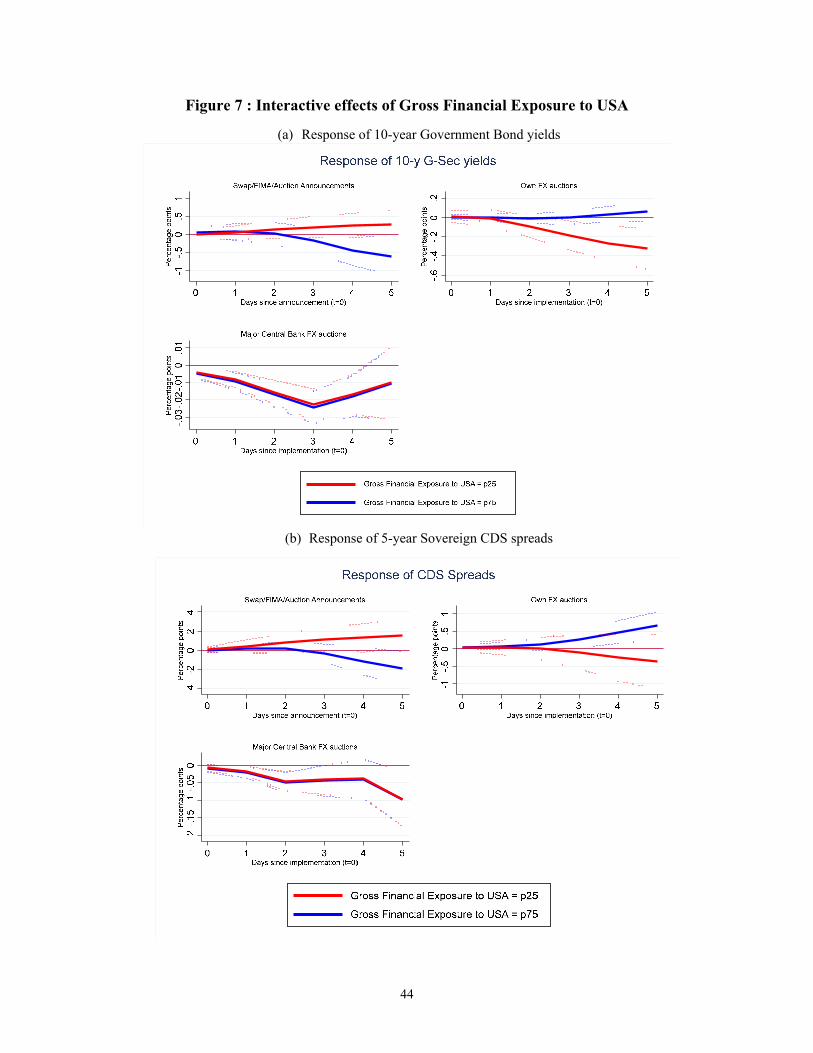
44

Figure 7 : Interactive effects of Gross Financial Exposure to USA

(a) Response of 10-year Government Bond yields

(b) Response of 5-year Sovereign CDS spreads

45

Figure 8: Interactive effects of foreign exchange exposure on CDS spreads

(a) Aggregate FX Exposure (higher values = greater short position in FX)

(b) Aggregate FX Debt Exposure (higher values = greater short position in FX)

Notes: The announcement takes place at t=0, and the cumulative impulse response functions are illustrated for the next five business days.

46

Appendix I: List of economies

Argentina Kazakhstan Trinidad and Tobago Aruba Kenya TunisiaAustraliaS Korea, Rep. S TurkeyAzerbaijan Kuwait UgandaBahamas, The Kyrgyz Republic Ukraine Bahrain Lebanon United Arab Emirates Bangladesh Liberia United KingdomS

Barbados Macao UruguayBelize Malaysia Venezuela, RB Bolivia Mauritius VietnamBosnia and Herzegovina MexicoS ZambiaBrazilS MoldovaBulgaria Morocco CanadaS NamibiaChile New ZealandS

China NicaraguaColombia Nigeria Costa Rica North Macedonia Croatia NorwayS

Czech Republic Oman DenmarkS Pakistan Dominican Republic Panama Ecuador Papua New GuineaEuro AreaS ParaguayEgypt, Arab Rep. Peru El Salvador Philippines Georgia Poland Ghana Qatar Guatemala RomaniaHaiti Russian FederationHonduras Saudi Arabia Hong Kong, China SingaporeS

Hungary South AfricaIceland Sri LankaIndia SwedenS Indonesia SwitzerlandS

Israel Taiwan Jamaica TajikistanJapanS Tanzania Jordan ThailandNote: The superscript “S” refers to the economies that are given swap lines with the Fed.

47

Appendix II: Data Sources

Below is the listing of the mnemonics for the variables used in the analysis, descriptions of these variables and the source(s) from which the primary data for constructing these variables were taken.

Variable Variable description Source 10-year G-Sec Yields Yield on 10-year government bonds, % Haver

ALLIANCE Dummy for economies that are in a formal military alliance with the US CIA Factbooks

AuctionMajor Total amount accepted in the day’s auctions of US dollars by the major central banks (ECB, BOE, SNB, and BOJ), in billions.. Websites of the sample economies’ central banks

AuctionOwn Amounts accepted in the day’s auction of US dollars by the economy’s own central bank, in billions. Websites of the sample economies’ central banks

BankExp

Claims of US banks on individual economies divided by the claims of US banks on all economies as of December 2019. Claims of US banks on all economies is constructing by summing the claims on individual economies for all economies for which data is available (i.e. it excludes the residual/unallocated amounts).

BIS Locational Banking Statistics

Absolute Basis Absolute value of the 3-month Cross-currency basis, i.e., deviations from CPI JP Morgan, Bloomberg and authors’ calculations

CDS Spreads Credit default swap spreads on sovereign senior 5-year bond. Refinitiv Datastream

Cuml_fx

Cumulative exchange rate change. The rate of change in the local currency value per dollar with respect to the average local currency value during the first two weeks of January 2020. Exchange rate is measured as local currency units per US dollar. Increase is a depreciation of the local currency.

Haver

d_AssetPurchases Dummy for days of announcements related to asset purchase programs by the economy’s central bank

Yale Program on Financial Stability https://som.yale.edu/faculty-research-centers/centers-initiatives/program-on-financial-stability/covid-19-crisis

d_Fiscal Dummy =1 when the economy’s authorities announce a fiscal policy response

Yale Program on Financial Stability https://som.yale.edu/faculty-research-centers/centers-initiatives/program-on-financial-stability/covid-19-crisis

D.FOREX Rate of depreciation for the nominal exchange rates in local currency units per US dollar. End of day values. Haver (WSJ and central bank rates)

d_Liquidity Dummy =1 when the economy’s authorities announce an asset purchase program Yale Program on Financial Stability

48

Variable Variable description Source

d_MacroPru Dummy =1 when the economy’s authorities announce a macroprudential policy action Yale Program on Financial Stability

FedSwap Dummy variable. Equals 1 if the economy received a Federal Reserve swap-line, 0 otherwise. Fed’s website

fx_vol Exchange rate volatility, measured by the standard deviations of the rate of depreciation over rolling 14-day windows. Haver

Global_Fin Level of global financial exposure, measured by economy i’s sum of external assets and liabilities as a ratio to the world’s external assets and liabilities over the period of 2005 through 2015.

Lane and Milesi-Ferretti (2001, 2007, and 2017)

Global_Trade Level of global trade exposure measured by the share of economy i’s sum of exports and imports in global trade (i.e., the world’s sum of exports and imports.

IMF Direction of Trade Statistics

Gross Portfolio Exposure to US

Gross portfolio exposure of country i to US using restated CPIS (methodology 3). Computed as (Economy i’s liabilities to US + Economy i’s Claims on US)/( Economy i’s Total Liabilities + Economy i’s Total Claims)

Coppola and others, 2021

Aggregate FX exposure

Aggregate foreign-currency exposures , variable FXAGG from Benetrix and others, Rebased to maximum = 0 in sample, i.e. Max(FXAGG)-FXAGG, so that higher values represent greater FX short position. Measrued as of last available value (2017)

Benetrix and others (2019)

Aggregate FX debt exposure

Aggregate foreign-currency debt exposures , variable FXAGG_debt from Benetrix and others, Rebased to maximum = 0 in sample, i.e. Max(FXAGG_debt)-FXAGG_debt, so that higher values represent greater FX short position in debt

Benetrix and others (2019)

IR_g International reserves minus gold Global Development IndicatorsKAOPEN Chinn-Ito index of financial openness Chinn and Ito (2006, 2008)

Lockdowns

Number of measures introduced/extended less number of measures phased-out, for the following types of measures: Border closures, closure of businesses and public services, complete border closures, curfews, domestic travel restrictions, full lockdowns, international flights suspension, isolation and quarantine policies, limit public gatherings, partial lockdowns, state of emergency declared.

ACAPS COVID-19 Government measures dataset: https://www.acaps.org/covid-19-government-measures-dataset

MOBILITY

7-day moving average of the change in mobility. The change in mobility is the percentage change from baseline, of workplace mobility from Google Global Mobility Report for all economies except China. For China, the Baidu city movement intensity data for Wuhan is used to construct the percentage change in mobility from the baseline of first two weeks in January 2020.

Google Global Mobility Report; Baidu City Movement Intensity data

49

Variable Variable description Source New COVID-19 cases

7-day backward looking moving average of new COVID-19 cases per million population Ritchie and others (2020)

Policy rate easing Decline in monetary policy rate Haver

QE Dummy for the implementation of quantitative easing (QE) by the Fed on March 23, 2020. Fed’s website

Ratings

Change in long-term foreign currency sovereign credit ratings by Fitch, Moody’s or Standard and Poor’s (S&P). The variable takes the value +1 on days that see a ratings upgrade by any of the agencies, -1 on days with a downgrade and 0 otherwise.

Fitch, Moody’s, and S&P

stk_vol Stock market return volatility, measured by the standard deviations of the rate of stock market total return over rolling 14-day windows. Haver

SwapFimaAnn

Dummy variable that takes the value of one on the days of Fed swap announcements for the swap recipients, and on the days that an economy announced it had been granted access to FIMA repo facility for that economy and on the days that an economy with access to Fed facilities announced that it would conduct US dollar auctions.

Fed and other central bank websites

TradeShare Total US goods trade with the individual economy as a share of US goods trade with the world in 2019. IMF Direction of Trade Statistics (DOTS)

Total COVID-19 cases

Total number of COVID-19 cases per million population Ritchie and others (2020)

Total_returns Daily total return of the benchmark stock market index (%) Refinitiv Datastream

US Major Announcements

Dummy = 1 on days of major US announcements, including days of FOMC announcements liste don the Fed website and major announcements during COVID-19 crisis listed in the source website.

https://www.americanactionforum.org/insight/timeline-the-federal-reserve-responds-to-the-threat-of-coronavirus/ Federal Reserve Board

USShareinTrade Share of US in the economy’s total exports and imports of goods and services in 2019 IMF DOTS

USD_share_Reserves Share of USD assets in total foreign exchange reserves Ito and McCauley (2019) and Chinn, et al. (2021)VIX Chicago Board Options Exchange Volatility Index (VIX) in log https://www.cboe.com/tradable_products/vix/

Weighted AuctionOwn Sum of the amounts accepted (in billion US dollars) in the day’s US dollar auctions weighted by the tenor of each auction. Weights are the tenor of each auction divided by the maximum tenor in sample.

Central bank websites

Weighted AuctionMajor

Weighted auctioned amounts by the four major central banks, with weights constructed as for Weighted AuctionOwn

Central bank websites

50

Appendix III: Correlation of the variables for the estimation on the size of US dollar auctions

Auction Cumulative

Deprec. Rate

Exch. rate volatility

Stock market

VolatilityVIX (in log)

US Bank Exposure, 2019Q4

New cases, MA

Mobility index, MA

Auction 1.000

Cumulative Deprec. Rate -0.047 1.000

Exch. rate volatility 0.061 0.621 1.000

Stock market Volatility 0.051 0.211 0.429 1.000

VIX (in log) 0.076 0.167 0.386 0.591 1.000

US Bank Exposure, 2019Q4 0.203 -0.110 0.040 0.035 -0.015 1.000

New cases, MA 0.015 -0.063 -0.016 -0.057 -0.058 0.064 1.000

Mobility index, MA -0.001 -0.193 -0.125 -0.179 -0.074 -0.044 -0.253 1.000

51

Appendix IV: Determinants of the size of US dollar auctions by central banks – Heckman Estimation (1) (2) (3) (4)

Reaction equation Cumulative depreciation rate -1.237 -1.149 -2.268 -1.657 (t-1) (0.536)** (0.727) (0.911)** (0.818)**

(Second estimation: Exch. rate volatility 8.556 8.874 19.686 15.947Estimation of the (4.381)* (6.403) (8.137)** (7.931)**

volume of auctions) VIX (in log) 33.084 43.144 19.298 20.421 (13.303)** (17.459)** (13.486) (13.064) US Bank Exposure, 2019Q4 77.650 126.223 126.631 133.751 (46.907)* (73.377)* (54.563)** (67.503)** Cumul. Deprec. Rate -4.603 -6.944 x US Bank Exposure (2.609)* (3.740)* Exch. rate volatility -2.325 9.809 x US Bank Exposure (25.640) (27.846)

Selection equation Cumulative depreciation rate -0.070 -0.068 -0.084 -0.065 (0.010)*** (0.012)*** (0.013)*** (0.015)***

(First estimation: Exch. rate volatility 0.474 0.477 0.661 0.559 Probability of (0.089)*** (0.099)*** (0.105)*** (0.115)***auctioning) Stock market volatility 0.103 0.105 0.082 0.085

(0.034)*** (0.034)*** (0.045)* (0.044)* VIX (in log) 0.966 1.004 0.136 0.227 (0.257)*** (0.261)*** (0.434) (0.445) US Bank Exposure, 2019Q4 6.298 6.848 5.434 6.388 (0.388)*** (0.740)*** (0.521)*** (1.075)*** Cumul. Deprec. Rate -0.059 -0.404 x US Bank Exposure (0.119) (0.155)*** Exch. rate volatility -0.506 0.872 x US Bank Exposure (1.006) (1.205) New COVID cases, MA 0.002 0.002 (0.001)* (0.001)** Mobility index, MA -0.002 -0.003 (0.002) (0.002)

/mills lambda 12.049 17.092 25.344 21.769 (9.257) (11.570) (12.309)** (11.260)*

N 5,350 5,350 2,830 2,830 R2 . . . .

# of countries 50 50 47 47

52