Embed Size (px)
Citation preview

·"I: ./·. !I i· }
PCI COURSE: SOUTH AFRICA, AUGUST 1988
by Dr. B. F. MCCULLOUGH
CENTER FOR TRANSPORTATION RESEARCH BUREAU OF ENGINEERING RESEARCH
THE UNIVERSITY OF TEXAS AT AUSTIN
Summary of the PCI Course on
Design of Concrete Roads: A Review of the 1986 AASHTO Guidelines
By Dr. B. Frank McCullough, Director
The Center for Transportation Research and the Adnan Abou-Ayyash Professor
of Civil Engineering
The primary purpose of this course is to present basic concepts
and applications for the revised AASHTO Guide for design of pavement
structures considering the following principles:
1) Introduction
2) Pavement design and management
3) General design concepts and input
4) Rigid pavement design procedure
5) Rehabilitation of flexible and rigid pavement with concrete
overlays
6) Implementation guidelines
Each of these principles and the introduction session are
discussed in more detail below.
The primary objective of the introduction session is to introduce
the participants to the Guide, with the following secondary objectives:
l) Provide the student with background on the development of the
Guide, organization of the material it contains and the
individuals contributing to its development.
2) Provide a conceptual overview of the Guide and the revisions
incorporated to provide the designer increased flexibility and
capability in design.
3) Provide the FHWA's viewpoint on implementing the Guide.

In the following
management principles.
session we will
The objective
discuss
of this
pavement design and
session will be to
familiarize the participants with the overall content of the Guide witt
special emphasis on the new or modified procedures and concepts which
have been added.
Emphasis will be given to the following items included in the
Guide namely: Glossary of terms, Roadbed soil strength, Inclusion of
environmental factors, Drainage, Pavement management, Reliability, and
Life cycle costs. Each of the listed topics will be further illustrated
by specific applications in each succeeding session.
The primary objective of the next session is to provide an
understanding of the design inputs of a general nature, i.e. applicable
to all pavement types. The secondary objective is to increase the
students capability to develop specific general input information for a
design problem.
Emphasis will be given to the analysis period, initial performance
period, roadbed soil resilient modulus, terminal serviceability index,
weighted -resilient modulus concepts, reliability, roadbed swelling,
roadbed frost heave, and pavement type. The approach used.will be to
explain the principles involved in developing the charts and their
application. Next, the procedures will be illustrated in step-by-step
applications to an example problems. Emphasis will also be given to
explaining the new concepts.
The objective of session 4 is to describe concepts related to the
use of the guide for the design of rigid pavements and to illustrate
design procedures by example problems. The design procedure will
encompass both the thickness design and horizontal dimensions such as
joint spacing, reinforcement, etc. Explanations will emphasize the type
of information required to design of pavement, sources of information
and interpretation of results that apply to specific examples. The
factors presented in Session 3 will be considered in discussing the

I ~ I
I
I I I
design procedure.
follows:
Specifically, the material will be covered as
1) Specific rigid pavement input
2) Rigid pavement thickness design
3) Rigid pavement joint design
4) Rigid pavement reinforcement design
5) Example problems
Computer aided examples will be used to illustrate specific design
procedures for new construction.
The 1986 Guide includes a procedure for evaluating existing
pavements to determine overlay requirements. Session No. 5 will review
concepts and illustrate procedures for estimating
concrete overlay requirements.
portland cement
The subjects to be covered in this session include the following;
methodology, unit delineation, remaining life, flexible overlays on
rigid existing, rigid overlays on rigid existing, rigid overlays on
existing flexible, use of recycled materials, and use of milling
procedures.
The primary objective of the final session is to encourage the
attendees to implement the Guides and provide basic procedural
guidelines for an agency to implement the new concepts. Illustrative
examples of the procedures that may be used by the States will be
provided. The basic problems will be defined, the agency needs will be
outlined, the alternate approaches or solutions will be covered, a basic
sample plan will be formulated to illustrate the concepts involved, and
the need for implementation will be emphasized.

Session 1
Introduction
Objectives
The primary objective of this session is to introduce the
participants to the Guide, with the following secondary objectives:
1. Provide the student with background on the development of the
Guide, organization of the material it contains and the
individuals contributing to its development.
2. Provide a conceptual overview of the Guide and the revisions
incorporated to provide the designer increased flexibility and
capability in design.
3. Provide the FHWA's viewpoint on implementing the Guide.
Outline
During this session, emphasis will be given to the following
items:
1. An introduction of the instructors, students, and the course
approach.
2. The agenda, objectives and scope of the sessions.
3. The background of Guide development. This will cover the
organization, individual contributors, process, etc.
4. The FHWA viewpoint on implementation as to schedule and use in
documenting designs (presentation by FHWA representative) .
5. A slide presentation providing a conceptual review of the Guide.
This will provide the student a short overview of the Guide with
emphasis on the new concepts incorporated, philosophical
considerations, the models used, and design comparisons.
6. A brief discussion of the limitations of various design methods
will be provided so that ,a fair comparison can be made. The
tendency is to critique the material at hand while holding a less
perfect method as a reference.
1.1

COURSE APPROACH
1. Familiarize a. Basic Concepts & Procedures b. Application · of Procedures c. Limitations
2. Implement a. Needs of Agency b. Me:hanistic
3. Computer Program
1.4

, TASK FORCE GUIDELINES
1. SS/ Ai' s from tests
2. Variability I Reliability
3. Emphasis on Reliability
4. Life cycle costs
5. Drainage
6. Provide for revisions
7. National & International in Scope
a.. Cities & Counties b. Other Agencies
c. Other co·untries
8. 2/3 Approval
1.5

l'l ...
HISTORICAL DEVELOPMENT OF GUIDES
1959 Guidelines
1962 - Interim Guides
1972 - Revision of Guides (Blue Manual) anq NCHRP Report 128
1 981 - Chapter Ill Revisions
1986 - Guide _,
1.6

LIMITATION OF GUIDE
1. Specific pavement materials and roadbed soil
2. Single ·environment
3. An accelerated two-year testing period . extrapolated to a 10 - 20 designs
-
4. Operating vehicles with identical axle loads and configurations, as opposed to mixed traffic
GENERAL LIMITATIONS
1. Verification
2. Inadequate statistical data ( reliability )
3. Definition of failure missing
1.7

\
en w ::c (..) <( 0 a:
en c.. c..
·--~ <( 0 en 0
-I 1-
1- c. 1- en <( w z z z (..) (..) w 0 - z (!J :::c :E en 0 - c. a. en - (.)
0 w a: 0 en c <( en --1 --1 a. 0 (.) w w
:E -I - c > ~ en - 0 w w O·J: <t c z (.) c. OJ ~

CONSULTANTS
PROJECT MANAGERS F. N. FINN & B. F. McCULLOUGH
I I I I Part I Part II Part Ill Part IV
TEAM LEADER: TEAM LEADER: TEAM LEADER: TEAM LEADER: W.R. HUDSON B.F. McCULLOUGH M.W. WITCZAK C.L. MONISMITH
P.E. IRICK R.G. HICKS M.l. DARTER M.l. DARTER
A. LeCLERC R.L. LYTTON J.EPPS

Improvements to the Guide
1. RELIABILITY
2. MR FOR SOILS
3. MR FOR LAYER COEFFICIENTS
4. DRAINAGE
5. ENVIRONMENT
6. LOAD POSITION
7. SUBBASE EROSION
8. LIFE CYCLE COSTS
9. REHABILITATION
10. PAVEMENT MANAGEMENT
11. LOAD EQUIVALENCIES
12. TRAFFIC DATA
13. LOW VOLUME ROADS
14. MECHANISTIC I EMPIRICAL DESIGN
1 1 n

en (J.)
=:: en 0
c I-(J.)
"C • -~ : :l -0 0 0 • en . J:: . I-~
N • (J.) ,... en ,...
"C II II • :l c "0 c • 0 (1)
J:: ·- en ... "C (J.) ·-t-
• 0 : • en -: t- l()
(J.) . U1 :I: N • =:: ~ en ,... 0
,... < II • c (.) II
(.) < c c c. •
1.11

0 0 1.0
~ ..J < (.)
a: c.. :: w
0 0 llll::t
0 0 C")
N'tfdS E>NIM
l. 12
(.)
1-en z < ::r: (.) w ::E -..J < (.)
a:
N
0 1.0 0 0') N
0 1.0 C")
0 M
en a: w <-' z w en en <( c.

INPUT MODELS OUTPUT
TRAFFIC FLEXIBLE PAVEMENT ENVIRONMENT RIGID STRUCTURE ...... . MATERIALS LVR COMBINATIONS
......
-t w
CONSTRAINTS REHABILITATION
ECONOMICS RELIABILITY . OPTIMUM SOLUTION

z 0 IC)
::I a: len z 0 (.)
><: ..J a: UJ > 0
c..-
I
/ I
I
~ z 0 -I-< a: 0 0: UJ 1-UJ c
X3GNI Allll8\f3~1AH3S
1 1 /,

..J ~ I
b--+1: t- I -C/) I I c. I
<J
>-~ UJ ....J
:2: c: UJ
I-> 0 C/)
-c U>o >-_ ....Jc: ~w Zc. <t
-c. c. ISd
1.15

o::t 1-<l
1-M <l
- - C\1
1-<l
,... 1-<l
~
' r
'
~
1 1 c.
-
-
-
CJ)
:I: 1-z 0 :! -

900 12,000 lb. wheel load
E:4.0x10 6 psi
800 k = 200 pci ....-... ·-(J)
c. ._... 700
en en ·w 600 c: t-en
500
:E EDGE WITH ::::> SUPPORT LOSS ~ 400
>< <(
300 :E
200 EDGE
100~--~----~--~----------~--~-1~
6 7 8 9 10 11 12
SLAB THICKNESS (in.)
1 . ] 7

8 10
-en c: 0 -(';3 (.) ·--0. 0. (';3
"C 7 ca 10
,0 -UJ EDGE WITH u.. SUPPORT LOSS
..J
1-z UJ :E 6 UJ 10 > <t
12,000 lb. wheel load c.. E = 4.0 X 1 06
· psi
k = 200 pci
6 7 8 9 10 11 12
SLAB THICKNESS '(in.)
1 1 R

900 12,000 lb. wheel load
E = 4.0 X 10 6 psi
- 800 k = 200 pci en c. - 700 en en w 600 a: ..... en
500
:E :::>
400 :E - EDGE >< -=: 300 :E
200 INTERIOR
I 100
6 7 8 9 10 11 12
SLAB THICKNESS (in.)
1. 19

-C/)
c 0 ..... ·~
(.)
0. 0. ~
'i:j ~ 0
..._....
w u... ..J
r-z W. ~ w > ~ 0..
8 10
7 10
6 10
6
INTERIOR
7 8 9
12,000 lb. wheel load 6 E = 4.0 X 10 psi
k = 200 pci
10 11 12
SLAB THICKNESS (in.)
1. 20

UJ (.) z <(
_t ..J a: ~ <( <( 1:: en > UJ
0 ..J en <( 1-
i 0 1-
(f) (f) c.. (f)
~ ...J w I c.- <
UJ 1 z z •
(.) lc :::.:.::
:::: z Q (.)
c: <( en
:I: ... w t 1- I 1-a: <(
> 1-
(f) z ::::> UJ ...J
(f) z Cl c.. 0 0 ::
I c.- ...J a. t c:
<: ~ I:: -1-1-0 ::E z z (.) en w
t ...J .. -I (f) w 0:::
1. 21

,_..
N N
ZR. So .Wr =(10 )·wr
Wr =FR. wT
RELIABILITY FR FLEXIBLE
50 1.0
85 2.8
95 5.3
99 10.6
RIGID
1.0
2.3
3.6
6.2

c.. (.) c: ..,
1.{) 0 1.{) 0 ,... ,...
("U!) SS3N:>i~IHJ. ~~d
l. 23
0 0 ,...
0 0')
0 co
0 ,......
0 (0
0 1.{)
...-.. ~ 0 ..._...
>-1-...J -cc c::x: -...J w c:

:I: a. <t c: ." 0 :E 0 z
z (/')
l. 24
...... c: Q.)
E c: 0 lo.. ·-> c:
UJ

,_. N \.11
INPUT
- THICI<NESS
• Time
• Traffic
• Reliability
• Environment
• PSI
• MR • Concrete properties
-CONFIGURATION
• Joints
• Reinforcement
Concrete properties
Steel properties
Subbase properties
(/) ,.....,_
c.. r I 1 I
\ bC/) I
-c C1)
E Q)
(/) ,.....,_
> c.. r_ en as c..
...J w \ c 0 ± :E
c >< <:]
0 (/)
0 ~
w
(/)
~ / (/) c.. ell I-
C1) ~ z en Q)
ell ;! f( - w .c ell
:E .c ::E
en ::l w en en (.)
w a: z 0 ~ u.. (.) z I>< -:I: w I- a:
1 '?h

z 0 -t-~ 1--
-I
L
-,
U> ..... c. Q.) (.) c: 0
(.)
I
-
-I -1
~c: ctSO
.... c= ....... (.)
"'C~ --Q.)0 u::u
L I -
1. 27
-I , I
c: ctS>. =ctS -... - ,...... J... J...Q.) a.>> :o 0
L- I -
- -,
>. ctS -..... J... ....... Q.)
> 0
L

r
Rehabilitation Selection
I Analysis
Unit
I I
Deflection Condition Survey
I I
Selection of Analysis Units
I Materials
Characterization
I Remaining
· · Life
I Thickness
Charts
I Overlay
Thickness
I

AASHTO Pavement Design Courses FHWA Presentation
Subject: FHWA's Policy on Pavement Design and Rehabi1itation
o FHWA published an Informational Notice in the Federal Register on April 24, 1985, outlining the FHWA rulernaking process and encouraging full and early public participation in the development of the new guide.
o Recently, AASHTO requested FHWA approval to allow the use of two new pavement guides on Federal-aid highway work (F. B. Francois' Apr.il 17 letter attached):
1. ''Guide for Design of Pavement Structures (1986)", and 2. "Guidelines on Pavement Management (1985)."
o FHWA is developing a position on pavement design and rehabilitation to be published in the Federal Register.
o FHWA's proposed position on pavement design and rehabilitation includes:
l. Adopt both AASHTO publications as "guides'' and not as standards. 2. It is desirable for each State to strengthen its pavement
management program. 3. It is desirable for each State highway agency to have a
comprehensive engineering process for the selection and design of new pavement structures and rehabilitation strategies, and pavement management based on AASHTO and FHWA guidelines and local performance. Design criteria could be based on the new AASHTO Pavement Guide or other appropriate design guides, and performance experience in the State.
4. It is desirable for each State to have a multi-disciplinary pavement team to evaluate pavement design and rehabilitation projects and to develop feasible alternatives.
o Both of the new AASHTO guides provides the users with flexibility. Therefore, each State's criteria and process may differ depending on climate, geography, materials, etc.
o FHWA will be working with each State in the development of its formal pavement design and rehabilitation process. Our goal is to find each State's process acceptable by July l, 1988.
1 ?Q
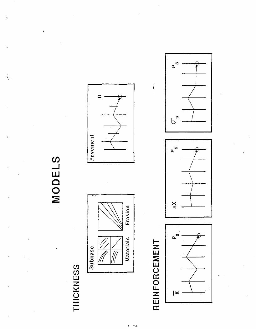
o Until our new pavement policy is adopted, we will continue to operate under our current policy which is:
Our field offices will continue using the 1972 AASHTO Interi;r1 Guide for Design of Pavement Structures (Chapter III ~evised 1~81) as the basis to evaluate the structural adequacy for pavement designs regardless of the design procedures used by the State. Our field offices have been asked to consult ~ith Headquarters regarding State requests to adopt the new Guide procedures prior to completion of the federal rulemaking process.
o When submitting designs under the new guide procedures during this interim period, it will expedite FHWA 1 s review if the data needed to compare the design to the Interim Guide procedures are also submitted.
Reorganization
Creation of a Pavement Division under Highway Operations with approximately 22 people ie. triple our current pavement staff. Division will be the primary focal point for pavement issues. Division made up of three teams: PM, PCC and AC. Pavement Management covers PMS as well as general pavement issues such· as equipment, trucks, and tire pressures. The other two teams will concentrate on Design and Rehaoilitation of flexible and rigid pavements. The reorganization plan will be implemented in August 1986.
Pavement Training
o Pavement Design Course (Four Days)
Significant need for pavement training, particularly on the new AASHTO Pavement Design Guide.
A comprehensive course on pavement design procedures including the new AASHTO guide.
o Study in Pavement Design, Rehabilitation, and Management Principles
This is the second generation of the 6-week Pavement Management Course held at the University of Texas.
Proposal is to contract for six 4-week sessions.
Have not yet solicited for Request for Proposals.
1 ")(')

NHI annual call for training is in progress. Contact FHWA Division Office or NHI.
o Techniques for Pavement Rehabilitation (3 l/2 Days)
This has been an extremely popular course now commonly known as Pavement 4R Course. 75 presentations have been given since January 1981 when course started. FHWA has 35 more presentations under contract that are available on request. Also, under consideration is the offering of 1-day modules on selected rehabilitation issues and techniques to States desiring specialized training. Interested States should contact the FHWA Division Office who will forward requests to the Washington Office.
o Pavement Seminar for State Executive Officers {1 Day)
This is primarily a second generation of the joint AASHTU/FHWA Pavement Seminar for Chief Administrative Officers held late last year in Clearwater, Florida and San Diego, California. · Material will be reorganized and aimed at the upper level of management. Work on this is just beginning and should be offered in 1987.
o Pavement Rehabilitation and Design Teams
To help support States implementation of the new AASHTO Guide, we plan to expand the scope of our current Pavement Kehabilitation Design Team concept. To date the team has visited approximately 27 States. We will provide technical assistance to State highway agencies and FHWA division offices in implementing the New Guide. This team concept will not be to review the State and make criticisms, but to assist with various aspects of rehabilitation and implementation of design procedures. Provide an outside opinion. The team will be customized to fit the particular expertise needed.
1 11

SESSION 2
Session 2
Part I · Pavement Design and Management
Principles
Objective
The objective of this session will be to familiarize the participants
with the overall content of the Guide with special emphasis on the new or
modified procedures and concepts which have been added.
Outline
Emphasis will be given to the following items included in the Guide:
1. Glossary of terms
2. Roadbed soil strength
3. Inclusion of environmental factors
4. Drainage
5. Pavement management
6. Reliability
7. Life cycle costs
Each of the above topics will be further illustrated by specific
applications in each succeeding session.
References
Reading material for this session will be found in Part f• Chapters 1
through 5. All resourse material used in the presentation is included in
the following pages.
Specific appendices of Part I (Vol I) which are related to this
2. l
Specific appendices of Part I (Volume I) which are related to this
session include: Appendices A, B, D, E, F, and G. In Volume II,
Appendices AA, BB, DD, EE, FF, GG, HH, and II provide additional
information for subjects included in this session.
2.2

DESIGN CONSIDERATIONS
1. PAVEMENT PERFORMANCE
2. TRAFFIC
3. ROADBED SOIL
4. MATERIALS OF CONSTRUCTION
5. ENVIRONMENT
6. DRAINAGE
7. RELIABILITY
8. SHOULDER DESIGN
9. PAVEMENT MANAGEMENT
10, LIFE CYCLE COSTS
2.3

GLOSSARY OF TERfS (PARTIAL)
ANA.L YS IS PER I OD - THE PERIOD OF TI~1E FOR ~IH I CH THE ECONQ'vl I C ANALYSIS IS TO BE
t1ADE; ORDINARILY WILL INCLUDE AT LEAST ONE REHABILITATION ACTIVITY.
DRAINAGE COEFFICIENTS - FACTORS USED TO MODIFY LAYER COEFFICIENTS IN FLEXIBLE
PAVEMENTS OR STRESSES IN RIGID PAVEMENTS AS A FUNCTION OF HOW WELL THE PAVEMENT
STRUCTURE CAN HANDLE THE ADVERSE EFFECT OF ~~ATER INFILTRATION,
EQUIVALENT SINGLE AXLE LOADS (ESAL'S) - SUMMATION OF EQUIVALENT 18000 POUND
SINGLE AXLE LOADS USED TO C~ffiiNE MIXED TRAFFIC TO DESIGN TRAFFIC FOR THE
DESIGN PERIOD,
LAYER COEFFICIENT (A1J A2J A3) ~ THE EMPIRICAL RELATIONSHIP Bffi/EEN STRUCTURAL
Nll'1BER (sN) AND LAYER THICKNESS WHICH EXPRESSES THE RELATIVE ABILITY OF A
1-tA.TERIAL TO FLNCTION AS A STRU::TURAL CO"'lPONENT OF THE PAVEMENT,
LOW VOLU.1E ROADS - A ROMJt'{AY GENERALLY SUBJECTED TO LOW LEVELS OF TRAFFIC; IN
THIS GUIDEJ STRUCTLRAL DESIGN IS BASED ON A RANGE OF 18-KIP ESAL' S FR0"-1
50J000 TO 1J000J000 FOR FLEXIBLE AND RIGID PA~~B~TS AND FROM 10JOQO TO
1JOQOJQOO FOR AGGREGATE SURFACED ROADS,
t10DULUS OF SUBGRADE REACTION (K) - WESTERGAARD'S fv'ODULUS OF SUBGRADE REACTION
FOR USE IN RIGID PAVEMENT DESIGN (THE LOAD IN POUNDS PER SQUARE INCH ON A
LOADED AREA OF THE ROADBED SOIL OR SUBBASE DIVIDED BY THE DEFLECTION IN INCHES
OF THE ROADBED SOIL OR SUBBASE) PSI/IN,)
PAV~1ENT PERFORMMJCE - THE TREND OF SERVICEABILITY WITH LOAD APPLICATIONS,
PERFORMANCE PERIOD - THE PERIOD OF TIME THAT AN INITIALLY CONSTRUCTED OR
REHABILITATED PAV8'1ENT STRUCTURE WILL LAST (PERFO~) BEFORE REACHING ITS
·TE~1INAL SERVICEABILITY; THIS IS ALSO REFERRED TO AS THE DESIGN PERIOD.
2.4

GLOSS4RY OF JE!ttS (PARTIAL)
RESILIENT t'QDULUS - A MEASLRE OF THE ~10DULUS OF ELASTICITY OF ROADBED SOIL
OR OTHER PAVEMENT MA. TER I AL,
ROADBED MATERIAL - THE MA.TERIAL BELOW THE SUBGRADE IN CUTS AND EMBANKMENTS
AND IN 8'1BN'li<MENT FOll-JDATIONSJ EXTENDING TO SUCH DEPTH AS AFFECTS THE SUPPORT
OF THE PAVEMENT STRUCTLRE,
TRAFFIC EQUIVALENCE FACTOR (E) - A NUMERICAL FACTOR THAT EXPRESSES THE RELATION
SHIP OF A GIVEN AXLE LOAD lD N'JOTHER AXLE LOAD IN TERMS OF THEIR EFFECT ON THE
SERVICEABILITY OF A PAVEMENT STRUCTURE, IN THIS GUIDE) ALL AXLE LOADS ARE
EQUA.TED IN TERMS OF THE EQUIVALENT NUviBER OF REPETITIONS OF AN 18-KIP SINGLE
AXLE,
2.5
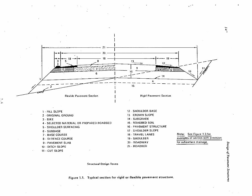
----j---1 I
Flexible Pavement Section 1
1 · FILL SLOPE
2 · ORIGINAL GROUND
3 ·DIKE 4 · SELECTED MATERIAL OR PREPARED ROADBED
5 • SHOULDER SURFACING
6 ·SUBBASE 7 · BASE COURSE
8 · SUflFACE COURSE
9 • PAVEMENT SLAB
10 - DITCH SLOPE
11 · CUT SLOPE
I
Structural Design Terms
14
4 -----15
Ri!Jid Pavement Section
12 · SHOULDER BASE
13 CROWN SlOPE
14 · SUBGRADE
15 · ROADBED SOIL
16 · PAVEMENT STRUCTURE
17 ·SHOULDER SLOPE
18 - TRAVEL LANES
19 - SHOULDER
20 ·ROADWAY 21 -ROADBED
Figure 1.1. Typical section for rigid or flexible pavement structure.
-
~ See Figure 1.3 ,for
examples of section with provision
for subsurface drainage. t;,
" .. o;;·
;::a
~
"' "" -c
" 3
" ;::a ... ~ ~ ... i: ;; ..

..c C"a Cl)
u
5
·- p ~ t ------------------------------Cl)
en
0
Criteria
pt
3.0
2.5
2.0
Traffic
for selection of
0/o Stating -Unacceptable
12
55
85
2.7
T .~PSI
~
pt • •

Appendix D
Table 0.23. Worksheet for calculating 1 8-kip equivalent single axle load (ESAL) application•.
Location Example 3
Vehicle Types
Passenger Cars Buses
Panel and Pickup Trucks Other 2-Axle/ 4-Tire Trucks 2-Axle/6-Tire Trucks 3 or More Axle Trucks All Single Unit Trucks
3 Axle Tractor Semi-Trailers 4 Axle Tractor Semi-Trailers 5 +Axle Tractor Semi-Trailers All Tractor Semi-Trailers
5 Axle Double Trailers 6 +Axle Double Trailers All Double Trailer Combos.
3 Axle Truck· Trailers 4 Axle Truck-Trailers 5 + Axle Truck-Trailers All Truck· Trailer Combos.
All Vehicles
CurTent Traffic
(A)
5,925 35
1.135 3
372 34
19 49
1,880
103 0
208 305 125
10,193
Analysis Period = 20
9" Assumed SN or D = ----
Growth Factors
(B)
4%
29.78 29.78
4%
29.78 29.78 29.78 29.78
6%
36.79 36.79 36.79
7%
41.00 41.00
6%
36.79 36.79 36.79
Design Traffic
(C)
64,402.972 380.440
12,337.109 32,609
4,043.528 369.570
E.S.A.L. Factor
(0)
.0008
.6806
.0122
.0052
.1890
. 1303
255.139 - .8646 657.989 .6560
25,245,298 2.3719
1,541.395 2.3187
2.793.097 4,095,647 1.678,544
.0152
.0152
.5317
Design
Years
o .. ion E.S.A.L.
(E)
51,522 258,927
150.513 170
764.227 48,155
220.593 431,641
59.879.322 *
3,574,033 *
42,455 62.254
892,482
1 17,833,337 E.S.A.L 66,376.294 **
* Note (1) These- two categories account for 96' percent of total E.S.A.L.'s calculated in this example.
** Note (2) Unfactored for direction and lane distribution (rnulti-laned facility).
2.8
D-'27

(f) (f)
~~ . t; I
c:~ 0 II .... ~~ > UJ c
SCHEMATIC DIAGRAM OF RESILIENT MODULUS TEST (AASHTO T274)
(h (AXIAL STRESS)
• • • • • • • •
• • • • •
• • • • • • •
• • SAMPLE ' a; './. · .. '
• • • • • (CONFINING STRESS) · • •
• • • • • • • • • •
t Ch
STRESS- STRAIN DIAGRAM MR
e (resilient) log Gd
f

NEED FOR SUBSURFACE DRAIN
BASED ON: ·,
• FREQUENCY OF RAINFALL
• AMOUNT OF RAINFALL
• QUANTITY OF WATER TO BE DRAINED
• THICKNESS OF DRAINAGE LAYER
• PERMEABILITY OF DRAINAGE LAYER
• HYDROSTATIC HEAD

ln.trodJ~ction and Bad:growui
A. Base is used as the drainage layer.*
Drainage layer as a base
Base and subbase material must meet filter criteria
Material must meet filter criteria
B. Drainage layer is part of or below the subbase.
Drainage layer as part of or b~>low the subbase
Base and subbase material must meet vertical drainage permeability criteria
filter criteria
Material must meet filter .criteria if base or subbase adjacent to draina~e-layer does not meet filter criteria ·
Note: Filter fabrics may be used in lieu of filter material, soil, or aggregate, oepending on economic considerations.
* Generally preferred configuration.
Figure 1.3. Example of drainage layer in pavement structure ( 11).
2. 11
1·19

Time reauired to drain 0 5 ft. 3 of water/ lineal foot of o 24 'wtde pavement I
2~:o"Roodwoy
=t H • Dislanct from Suooast to 1116 ~ waltrlab/6.
------ - · · ...... Ho•HtJir;llt of Drain abov;-;;;;--im~rvious boundry
PERMEABILITY
Ratio H/Ho ,o·JCM/SEC t0-4r:M/SEC 10-6CM/SEC I0-6 CM/SEC 2.8 A/Ooy 0.28FI./Oay 0.028 Ft./Day O.CXJ28 Ft./Day
0.0 Minutes Hoc;rs Days Wuks
0.1 108 /8 1.4 10.5
0.2 54 9 3.8 5.3
0.3 35 5 2.5 3.5
0.4 21 4.5 /.9 2.5
0.5 24 3.8 1.5 2.1 0.5 21 3.0 1.3 1.8
O.T 18 2.5 1.1 1.5 0.8 15 2.2 0.9 1.3
0.9 /3 2.0 0.8 1.2
/.0 10 1.8 0.1 1.1
Chart Based on OARCYS LAW In Form of 0.5 T.: K 'fHo A
T = Time( Days) H = Hydraulic Head In Ft.
,o-TCM/SEC IOCXJ028Ft/Doy
Montns
24.8 12.4
8.3 6.2
5.0 4.1
3.5
3.1
2.8
2.5
Ho= Depth of "Soil Reservoir" Overlyinq Impervious. Loyer, Fl .. A = Area, 24 Ft.2
BAS£ DRAINAGE TIM£ VARIOUS SUBGRAO£ PERMEABILITY
Figure 7.
Note: Additional details regarding vertical drainage are prov~ded in Volume 2, Appendix AA.

( o}
K~~P joints os well /- sealed os possib/8
---_;_.;~~~;.;..:...:...:::~..._Pipe
Open-groded
--
(b)
(c)
(d)
(e)
bos~
Open- graded bose
Open-qroded Subbase bose
AC or PCC -'-
drain with pipe
I
Typical details of outer edges af drainaqe systems.
or bose
-----Outlet
OPEN GRADE BASE DESIGN
Figure 17.
Note: Additional details regarding drainage designs are provided
in Volume 2, Appendix AA.
') 11.
--·---

DRC\IN~GE F0~·1ULA
vlrlERE:
t 50 = TIME FOR 50 PERCENT OF LNBOLND WATER TO mAIN (DAYS)
n e = EFFECTIVE POROSITY (so PERCENT OF ABSOUITE POROSITY)
L = LENGTH OF FLOW PATH (FEET)
K =PERMEABILITY CONSTANT (FT/DAY), AND
H = THICKNESS OF DRAINAGE LAYER
TAN a = SLOPE OF THE BASE LAYER
I I I I I I I I I I I I I I I I I I I I I I I I I I I I I I I I I I I I I I
SLOPE OF BASE LAYER
sl=VSrz+sL2
WHERE: ST2
=SLOPE IN TRANSVERSE DIRECTION
2 SL = SLOPE IN LONGITUDINAL DIRECTION
LENGTH OF FLOW PATH
'M-IERE: W = WIDTH OF LANE(S)
2.14

QUANTITY OF WATER INFILTRATING PAVEMENT
Q. = DESIGN INFILTRATION RATEJ FT 3fDAYfFT 2 OF DRAINAGE , LAYERJ.
3 IC = CRACK INFILTRATION RATEJ FT /DAY/LINEAL FOOT OF CRACK -
USE 2.4 UNLESS OTHER INFORMATION IS AVAILABLE
NC = NUMBER OF CONTRIBUTING LONGITUDINAL CRACKS
We = LENGTH OF CONTRIBUTING TRANSVERSE CRACKS OR JOINTS
W = WIDTH OF BASE OR SUBBASE SUBJECTED TO INFILTRATION) FEET
WC = SPACING OF TRANSVERSE CRACKS OR JOINTS) FEET s
Kp = CO~FFICIENT OF PERMEABILITY THROUGH UNCRACKED PAVEMENT) FT /DAY/SQUARE FOOT OF PAVEMENT
NOTE: ALTERNATE VALUES FOR Ic MA.Y BE FOLND IN LITERATURE AND JUSTIFIED BASED ON LOCAL EXPERIENCE,
2.15

DRAINAGE EXAMPLE
ASSUME:
7] = . 15
Tje = 0.81]= .12 PERCENT
L = 24 FEET
K = 1000 FTIDAY
H = 0.5 FT
TANct = 0.015 FOR 1 1/2 PERCENT TRANSVERSE
t 50 = C.12 * 242) I C2 * 1ooo) Co. 5 + 24 * o. 015)
= 69.12"/ (2000) (0.86)
= .04 DAYS
= 1 HOUR
'i , c.
I

QUALITY OF DRAINAGE
EXCELLENT
GOOD
FAIR
POOR
VERY POOR
* L = 24 FT.
H = 0,33 FT.
DRAINAGE PARAMETERS
WATER REMOVED WITHIN
0,083 DAYS(2 HOURS)
1 DAY
7 DAYS (1 WEEK)
30 DAYS (1 MONTH)
2.17
1202
100
14
3

1·20 Design of Pavement Structures
Table1.1. Permeability of graded aggregates (JJ).
Sample Number Percent Pauing 1 2 3 4 5 6
3..4 • inch sieve 100 100 100 100 100 100
V:! • inch sieve 85 84 83 81.5 79.5 75
¥a - inch sieve 77.5 76 74 72.5 69.5 63
No.4 sieve 58.5 56 52.5 49 43.5 32
No.8 sieve 42.5 39 34 29.5 22 5.8
No. 10 sieve 39 35 30 25 17 0
No. 20 sieve 26.5 22 15.5 9.8 0 0
No. 40 sieve 18.5 13.3 6.3 0 0 0
No. 60 sieve 13.0 7.5 0 0 0 0
No. 140 sieve 6.0 0 0 0 0 0
No. 200 sieve 0 0 0 0 0 0
Dry density (pcf) 121 1 17 115 1 1 1 104 101
Coefficient of permeability (ft. per day) 10 1 10 320 1,000 2.600 3.000
Note: Compare to criteria on page 2.17.
?. lR

1-)4
PLANNING ACTIVITIES
•
•
•
Assess Network Deficiencies
Establish Priorities·
Program and Budget
.. ~
A I I I l l I I I I
Research Activities
...
+ I I
I I I I I I I I I I I l I I l I I I
--..l.
Design of Pavement Srructures
DESIGN ACTIVITIES
Input Information on Materials, TraHic, Climate, Costs, etc.
_ ... Q-P'
Alternative Design Strategies
~ Analysis,
Economic Evaluation, and Optimization
,, +i Construction Activities
n
+i Maintenance Activities
.... H_ Pavement Evaluation
~ Rehabilitation Activities
Figure 2.2. Major classes of activities in a pavement management system.
2.19
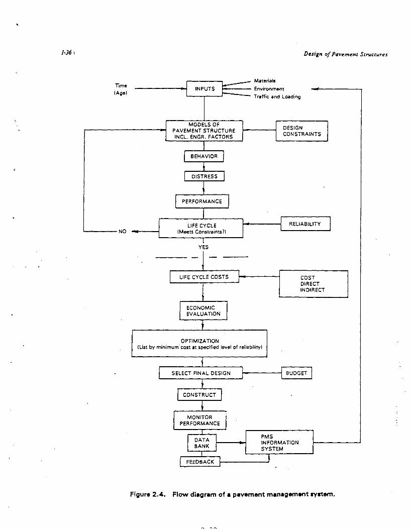
1·36t
Time (Agel
L....----NO
Design of Pavement Structures
Materials
1 INPUTS
I-Environment
- Traffic and Loading
MODELS OF DESIGN PAVEMENT STRUCTURE
INCL. ENGR. FACTORS CONSTRAINTS
I BEHAVIOR J
I DISTRESS J
I PERFORMANCE I J RELIABILITY I LIFE CYCLE I
(Meets Constraints71
I YES
- -
l LIFE CYCLE COSTS L COST I DIRECT INDIRECT
I ECONOMIC I EVALUATION
OPTIMIZATION (List by minimum cost at specified level of reliability)
SELECT FINAL DESIGN I : BUDGET I
I CONSTRUCT I
I MONITOR I PERFORMANCE
I DATA l PMS
BANK I INFORMATION SYSTEM
I FEEDBACK I ~
Figure 2.4. Flow diagram of a pavement management system.

LIFE CYCLE COSTS
1. SUMMARIZES ALL COSTS AND BENEFITS
t ENGINEERING AND ADMINISTRATION
t CONSTRUCTION
I MAINTENANCE
t USER
t SALVAGE VALUE
2. ECONOMIC COMPARISON
1 PRESENT WORTH
1 EQUIVALENT UNIFORM ANNUAL COST
t DISCOUNT RATE
I ANALYSIS PERIOD
? ?1
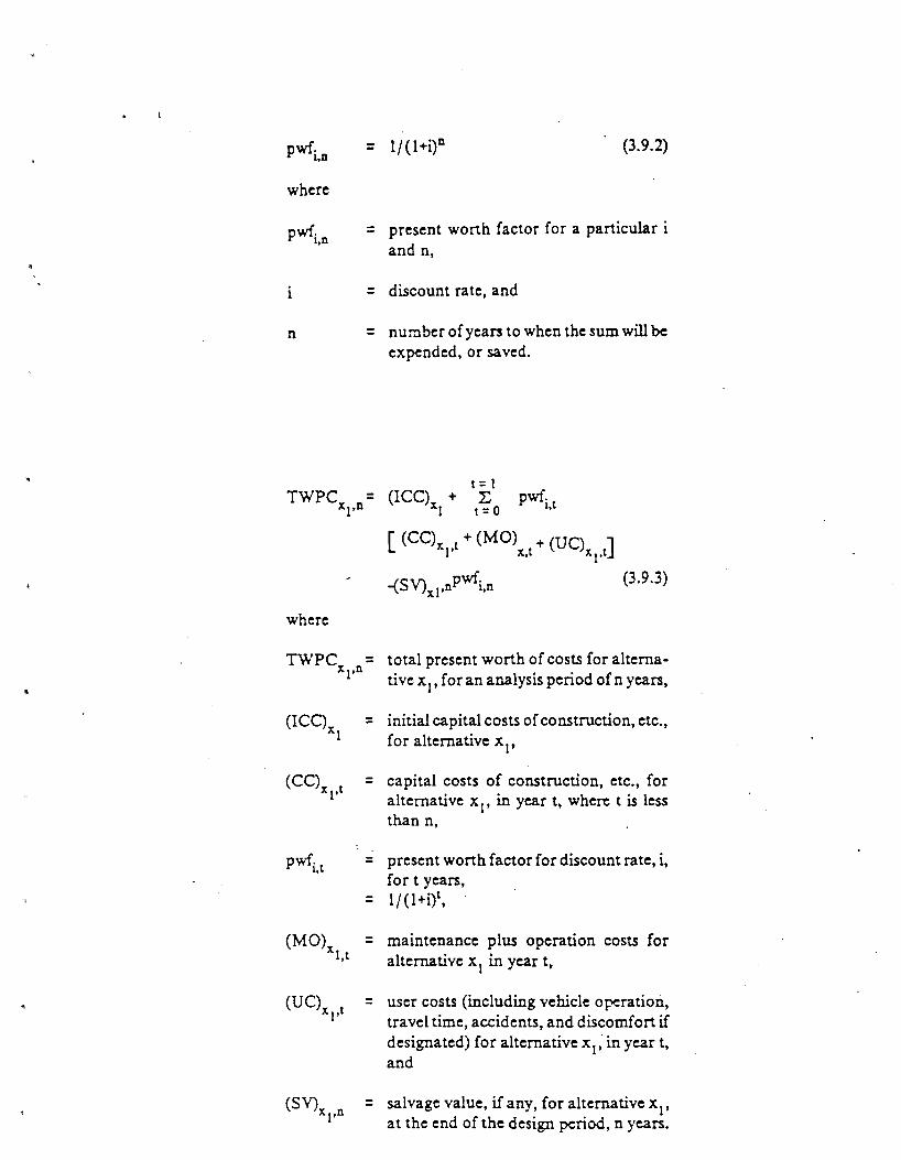
pwf. = 1/{l+i)n (3.9.2) 1,n
where
pwf. = present worth factor for a particular i 1,n and n,
= discount rate, and
n = number of years to when the sum will be expended, or saved.
t = 1 TWPCx
1,n= (ICC)x + ~ pwf.
1 t = 0 l,t
[ (CC)x t + (MO) + (UC) ] 1' x,t xl't
-(SV)x1.nPwfi,n (3.9.3)
where
TWPCx n = total present worth of costs for alterna-1' .
(CC)x t 1'
(MO)x 1,t
(UC)x t 1'
(SY\ n 1'
tive x1, for an analysis penod ofn years,
= initial capital costs of construction, etc., for alternative x 1,
= capital costs of construction, etc., for alternative x1, in year t, where t is less than n,
= present worth factor for discount rate, i, fort years,
= 1/(l+i)t,
= maintenance plus operation costs for alternative x 1 in year t,
= user costs (including vehicle operation, travel time, accidents, and discomfort if designated) for alternative x1; in year t, and
= salvage value, if any, for alternative x1,
at the end of the design period, n years.

LIFE CYCLE COST EXAMPLE
ASSUME:
INITIAL CONSTRUCTION COST: $45~00/SQ,YD,
FIXED COSTS: $15.00/SQ,YD,
ANNUAL MAINTENANCE YEAR 5 $ 0.02/SQ,YD,
ANNUAL INCREASE $0.005/SQ,YD,
COST OF OVERLAY $10.000/SQ,YD,
SALVAGE VALUEJ 70% $31.50
,, ANALYSIS PERIOD 15 YEARS
DISCOUNT RATE 4 PERCENT
YEAR COST PWF PW
0 45 1.0 45.00 * 5 0.02 0.806 0.02
6 0.025 0.775 0.02 7 0.030 0.745 0.02 8 0.035 0.716 0.03
* 9 0.040 0.689 0.03 10 10.000 0.662 6.62 15 (sv) .70 X (45 + 10) 0.545 20.98
NPW = 51,74- 20,98 = $30.76
* $141/LANE MILE EQUIVALENT TO ,.
2.23

DEFINITION OF RELIABILITY
RELIABILITY IS THE PROBABILITY THAT A DESIGNED PAVEMENT SECTION WILL PERFORM SATISFACTORILY FOR THE TRAFFIC AND ENVIRONMENTAL CONDITIONS EXPERIENCED DURING THE DESIGN PERIOD.

•
INCORPORATION OF RELIABILITY INTO AASHTO PAVEMENT DESIGN GUIDE REPLACES <IN-PART):
*. REGIONAL FACTOR IN FLEXIBLE PAVEMENT DESIGN CR TERM IN PERFORMANCE EQUATION)
* WORKING STRESS IN RIGID PAVEMENT DESIGN
(f t = sc';c IN PERFORMANCE EQUATION)
2.25

MAJOR SOURCES OF VARIATION THAT AFFECT PAVEMENT DESIGN AND/OR PERFORMANCE
* CONSTRUCTION CTHICKNESSES~ STRENGTHS~ ETC.)
* ENVIRONMENT CSOIL~ CLIMATE~ ETC.)
* TRAFFIC FORECASTS (PROJECTIONS)
* PREDICTION ERROR CERROR IN PERFORMANCE PREDICTION MODEL)
NOTE: THE AEOVE SOURCES OF VARIATIC('J HAVE BEB'i INCORPORATED IN THE RELIABILITY FACTOR FOR INITIAL DESIGN OR OVERLAYS,
2.26

USE OF MEAN (OR AVERAGE) VALUES FOR DESIGN
TEST NO. sc (psi)
1 521 MEAN II II 2 548 VALUE = 627
3 592 4 614 STD. 5 625 a= - 62 DEV. 6 636 7 649 90°/o 8 671 CONF. =~
~ 9 693 LEVEL 10 720 VALUE
, MEAN z ( ) ( Sc )d= VALUE- a
APPLIES TO ALL DESIGN FACTORS, INCLUDING :
• TRAFFIC • ROADBED SOIL STRENGTH • PAVEMENT MATERIAL PROPERTIES ·
• • LAYER THICKNESSES
Note: All input design factors must be based on averag·3 values with no adjustment based on distribution.
2.27

Table 2.2. Suggested I eve Is of reliability for various functional classifications.
Functional Classification
Interstate and other freeways
Principal Arterials
Collectors
Local
Recommended Level of Reliability
Urban
85 - 99.9
80 - 99
80 - 95
50 - 80
Rural
80 - 99.9
75 - 95
75 - 95
50 - 80
Note: Results based on a survey of the AASHTO Pavement Design Task Force
? ~~

(-lo5Fr)/5o:: 2-R
lo5 FR. = -r~ So .- 10 -c.JI:.S., r" ... =
NOTE i. The. '1./.:~lt..u! ... of C..,:: b dcfermine.d by +he. VAlue... of R 1
and i~ ob+Ainc..d -frorr1 ~ndard norTI'Ia I (...urve. ~n!C(
t-Pbk.~ by errkr-inj (100-R"/o)/100 for +h~~i/ a,...~ from - oa +o .Z:.. R .
NOTE Z. T f loj FP\ = o, C:R. = o, FR. ::r-l, and. R~s-o "/o. Thu:=. +he.. proba.bi/if.-[ for d~:jn period. :::;urviva{ i~ 50°/o. r+ -th'- tn~.ff,·v p~d,·c..-h'on ( w-;-) i~ 6ub~+i-h..Jf.ed dir-e.c:-+lt for Wt rn -t'h~ ~rfor-rna~ predic..ficr~ ( d~stj n) eauo::~:hon.
l
NOTE .3. fOr flx.e..d R. (henc::.e. fixd C.R}, FR. ,(-,c.-rease.s {orde....c...re.M~e..s) a.=, So= Js:...,.. t 5 N ,;,c..r~ase..::. (o ..... d~c..r'a~. f~ a.u.-ounb -For -+he.. :±o:ba..L ch.ane4".. vacla±ian tn -tr~f-fl"c..- pn:.did-jon.5 .E..!J..i_ perfor-manC/e--prtiioh'on6.
2.29

R
50 0
70 -.524
80 -.841
90 -L2e2
95 -1.64
99 -2.32
99.9 -3.09
RELIABILITY FACTOR FOR SPECIFIC
LEVELS OF RELIABILITY
0.34 0
0.34 < 1782
0.34 -.2589
0.34 -.4359
0.34 -.5576
0.34 -.7888
0.34 -1.0506
-z·*s 10 R 0.
1
1. 51
1. 93
2.73
3.61
6.15
11.24
.% I NCR EASE
1
51 1. 51
25
1. 93 ., .
41 ..
2.73
32 3.61
70 6. 15
83 11.24

SESSION 3

Session 3
General Design Concepts and Input
Objective
The primary objective of this session is to provide an understanding
of the design inputs of a general nature, i.e. applicable to ali pavement
types. The s~condary objective is to increase the students capability to
develop specific· general input information for a design problem.
Outline
Emphasis will be given to the following items:
1. Analysis period
2. Initial performance period
3. Roadbed soil resilient modulus
4. Terminal serviceability index
5. Weighted resilient modulus concepts
6. Reliability
7. Roadbed swelling
8. Roadbed frost heave
9. Pavement type
The approach used will be to explain the principles involved in
developing the charts and their application. Next, the procedures will be
illustrated in step-by-step applications to an example problems. Emphasis
will also be given to explaining the new concepts.
1 . 1

References
Reading material for this session will be found in Part II,
Chapters 1 and 2. The following references will also be of assistance:
1. Van Til, C.J., McCullough, B.F., Vallerga, B.A. and Hicks,
R.G., "Evaluation of AASHTO Interim Guides for Design of
Pavement Structures," NCHRP Report 128, 1972.
2. Rada, Gonzalo and Witczak, M.W., "A Comprehensive Evaluation of
Laboratory Resilient Moduli Results for Granular Material," TRB
Paper, 1981.
3. McCullough, B.F. and Elkins, G.E., "CRC Pavement Design
Manual," Austin Research Engineers, Inc., October 1979.
4. Carey, W. and Irick, P., "The Pavement Serviceability
Performance Concept," Highway Research Record 250, 1980.
In addition to this material, Appendices EE, FF, HH, II, and MM of
the Supplementary Information to the Guide will be used.
The following figures and tables in the Guide will be used during
the presentation and are listed in the order of presentation: Table
2.1, page II-5 and II-6; Figure 1.5, page I-28; Figure 1.4, page I-25;
Figure 2.3, page II-15; Figure 2.4, page II-16; Figure I-3, page I-10;
Figure 1.2, page I-10; Figure G.3, page G-4; Figure G.4, page G.7;
Figure G-7, page G-10; Figure G.8, page G-11; and Figure 2.2, page II-
11.
The student should review these items in advance.
3.2

FLOW DIAGRAM OF SCREEN PROGRAM
GENERAL INPUT
,...--(_P_av_ed_) _ __.I 1~--. __ (A_g_gr_e_ga_te_s_u_rf_ac_e---.)
I
PAVED ROAD CHARACTERISTICS
AGGREGATE
r-------J I SURFACE
(Flexible) (Rigid)
No
FLEXIBLE Overlay RIGID PAVEMENT ---,~ PAVEMENT
Overlay
Overlay
OVERLAY OVERLAY
OUTPUT
3.3

GENERAL INPUT
Problem Number & Description
1
General Design Inputs
2
Roadbed Soil Moduli
3
Paved I Aggregate Surface Road Switch
4

PAVED ROAD CHARACTERISTICS
Paved Road Swelling, Frost Characteristics Heave Data
P-1
Initial· Pavement
P-3
3.5
P-2

PSD-02
PSD-02 AASHTO PAVE~ENT STRUCTURAL DESIGN PROGRAM
VERSION 02 - APR. 1986
Prepartd For AMerican Association of Statt Highway
and Transportation Officials
Under Contract With National Cooperative Highway Research Program
Transportation Research Board Nat1onal Research Council
NCHRP Project 20-7/29
E I E . By . C lt t AR nc - ng1neer1ng onsu an s
Prttl Any Kty to Continue •••
!~PORT/CREATE DATA FILE
DATA FILE TO IMPORT I I I I I I I I I
This allows tht user to i•port and edit an existing data filt. This ~ay bt left blank if a new file is to be creattd.
DATA FILE TO CREATE AND AN~LYZE I
If left blank, a default na•t CPSOTEMP.OAT) will bt assu4ed,
3.6
I I I STEYE.RR
I I I STEYE.RR

PSD-02
PROBLEK NUK8ER AND DESCRIPTION
PROBLEM NUMBER ....... . ..... PROBLEM DESCRIPTION EXAMPLE APPLICATION OF AASHTO PAVEMENT STRUCTURAL DESIGN PROGRAM - RIGID INITIAL WITH RIGID OVERLAY
200b
F1r HELP F2r IMPORT/STORE F3r ANALYZE/PRINT/EXIT F~1 DISPLAY RESULTS
PSD-02
t t t SEHERAL DESIGN INPUT REQUIREMENTS t t t
ANALYSIS PERIOD <YEARS)
DISCOUNT RATE <Xl I I I I I I I t t I I
I I I I I I I I I I I
NUMBER OF TRAFFIC LANES <ONE DIRECTION) . LANE WIDTH <FEET)
30.0
~.00
2
12.00 COMBINED WIDTH OF SHOULDERS <FEET, ONE DIRECTION) 16.00
No.
F1r HELP F2r IMPORT/STORE F3r ANALYZE/PRINT/EXIT F~r DISPLAY RESULTS
3.7
200b

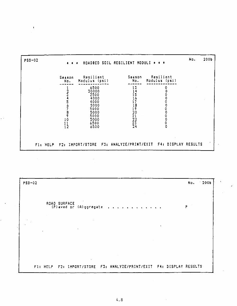
PSD-02 No. 200b I I I ROADIED SOIL REBILIEHT "ODULI t t t
Se&son Resilient Se&son Resilient No. Modulus (pI i ) No. Modulus (pI i ) ------ ------------- ------ -------------1 6~00 13 0
2 30000 14 0 3 2:500 1~ 0 4 4000 16 0 ~ 4000 17 0 6 :5000 18 0 7 :5000 1 9 0 8 5000 .20 0 9 :5000 21 0
10 :5000 22 0 11 6:500 23 0 12 6!500 24 0
Fl1 HELP F21 IMPORT/STORE F:S1 ANALYZE/PRINT/EXIT F41 DISPLAY RESULTS
PSD-02 No, 200b
ROAD SURFACE (Plaved or <Alggreg•t• p
F1t HELP F21 IMPORT/STORE F:S1 ANALYZE/PRINT/EXIT F4• DISPLAY RESULTS

REASONS FOR ADOPTING M R
1. Not identified with any specific agency
2. Fundamental engineering property
3. Techniques currently available for characterizing MR using NDT
4. M R now a standard test procedure
5. If initial equipment investment is · too high, possible to use correlation with other laboratory test
6. Favorable comparisons with other laboratory tests (U.S. Forest Service Study)
7. M R test is not too complex; familiarity and experience should reduce current problems with application
8. Reservoir of information
3.9

'l:t' 1-<J
f-M <J
N 1-. <J
T""
1-<J
..
---
r
'
3.10
en :z:: 1-z 0 ~
N ,..
-
...
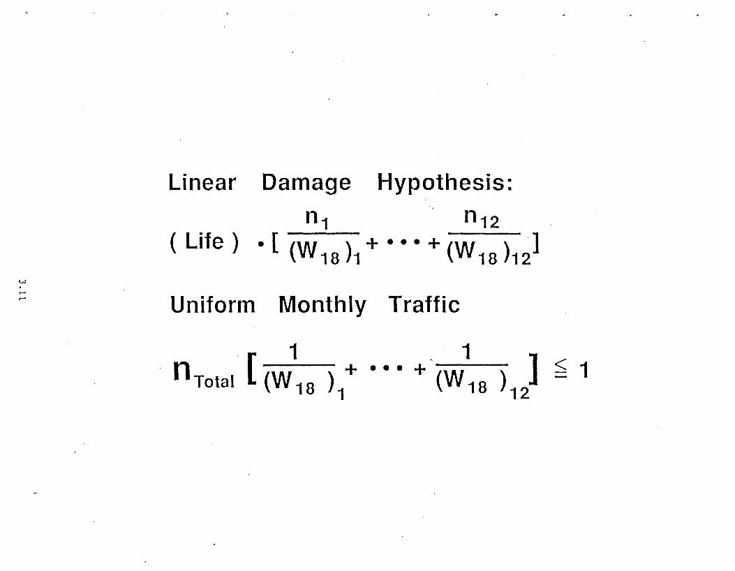
Linear Damage Hypothesis:
n1 n12
( Life ) • [ {W 18 )1 + • • • + {W 18 )1)
Uniform Monthly Traffic
. . 1 1 . nTotat ( {W
18 >/ • • • + --(W-1s-)
1) :::: 1

AASHO Equation :
k1 k2 2.32 W18 = SN •(p 0 ,p1 ,SN) ·MR
Damage Equation :
k 1 1 ] n S N k1
( p p SN) 2 ( 2.32 + • • • + 2.32 .:::_ 1
T • 0 ' t ' ( M R ~ ( M R )1 2

Inherent Reliability of AASHTO Interim Guide
Flexible Pavements -·
50 °/o reliability
Rigid Pavements (assume Pt = 2.5 )
Prior to 1981: .'·: ft = 0.75 • Sc
.•. Wt~ 8
= 0.374 W t; 8
( corresponds to approx. 85°/o reliability )
Since 1981:
• for C = 1.33 ( same as ft = 0.75 •Sc)
Wt~ 8
= 0.374 W t; 8 ( approx. 85°/o )
• for C = 2.00 Cft = 0.50•Sc)
Wt~ 8 = 0.093Wt; 8
( corresponds to approx. 98°/o reliability )
3.13

Predicted
s a-
mean value
k,D,E
3.14

..
en o_
en o_
Nl8
--""" ' .......
'
-' '
--
' ---------~--nK)
3.15
n50
no . es1gn
'

(f) 0...
z (f)
------- - -' ' ' ' ___________ ~ ~O- _ nOQ. ~n_oo_
Reliability
3. 16

0 0
0 co
II
z (/)
rr> II
z (/)
0 0 (!) v saJnf!D.:J <J'o
3.17
0 C\J
0
(J')
c 0
-+--0 (.)
c. c. <!
0 :::s
-+--(.)
<(
I
c 01 o-

• II :I:
w :: II
w "'C
Cl.) (.) Cl.) .Q (.) en -c c. ca
al .c .c 0 ::s c: en
':l 1 Q
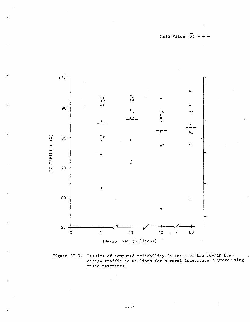
Mean Value (X)
100
0
0 oo 0 0 oo 00
oo 0
90 0 0 0 0 Oo
0
_OJJ_ 0 0 0
0
0 oo - 00 N 80 - 0 0
;:-... E-< ~
,....l ~
=:l < ....... ,....l w ~
00 0
0
0 0
70
0
60 0
0
50 -+------+----v' 1.--~:.---. 0 5 20 40 80
18-kip ESAL (millions)
Figure 11.3. Results of computed reliability in terms of the 18-kip ESAL design traffic in millions for a rural Interstate Highway using rigid pavements.
3.19

w
'" 0
FUNCTIONAL
CLASSIFICATION
INTERSTATE, FREEWAYS
PRINCIPAL ARTERIES
COLLECTORS
LOCAL
RECOMMENDED LEVEL OF RELIABILITY
URBAN RURAL
85 - 99.9 80 - 99.9
80 - 99 75 - 95
80 - 95 75 - 95
50 - 80 50 - 80

·•
ENVIRONMENTAL MODEL(S)
!J. PSI· = !J. PSI Traffic + !J. PSI Envir.
where: !J. PSITraffic = serviceability loss due to traffic which considers seasonal changes in subgrade support (i.e. resilient modulus, MR ) .
.6. PSI E · = serviceability loss due nv1r. to subgrade swelling and frost heave.
3.21

jj_ PSIEnvir. = ~ PSisw + 11 PSIFH + /1PSI0
. where: ~ .PSisw =
~ PSIFH =
serviceability loss due to subgrade swelling ·
serviceability loss due to frost heave
serviceability loss due to others factors defined by_ the state e. g. "D cracking"
3.22

H (f)
0...
P· I
p. I
p. I
Analysis Penod
Time
Analysis Period
Time
--- ....---02 ---
Analysis Period
Time
3.23
---
{j PSI Load
~PSITotal
....... .......
.......

.Appendi<r G
MOISTURE SUPPLY
NOTES:
G-3
HIGH FRACTURED
B ROADBED SOIL FABRIC
A
LOW TIGHT
al LOW MOISTURE SUPPLY:
Low rainfall Good drainage
b) HIGH MOISTURE SUPPLY
High rainfall Poor drainage Vicinity of culverts, bridge abutments. inlet leads
c) SOIL FABRIC CONDITIONS !self explanatory)
d) USE OF THE NONOGRAPH
1 l Select the appropriate moisture supply condition which may be somewhere between low and high (such as Al.
21 Select the appropriate soil fabric (such as B l. This scale must be developed by each individual agency.
31 Draw a straight line between the selected points lA to 8 l.
4) Read swell rate constant from the diagonal axis (read 0. 10).
Figure G.2.- Nomograph for estimating swell rate constant. Part II ( 1).
':\ ')I,
#-

5.0 ,-----;:==============~-------,
X w Cl z
>I-
3.0
:J CD <t w 2.0 u > a:: w C/)
1.0
Swelling Probability = 1.0
PVR= i" Swell Rote Constant = 0.04
Swell Rote Constant = 0.20
Swell Rote Constant = 0.20
® OVERLAY REQUIRED
5 10 15 20
TIME (YEARS)
Figure 6.4: PERFORMANCE CURVES ILLUSTRATING SERVICEABILITY LOSS NOT CAUSED BY TRAFFIC
3.25

J
One Section:
P{ Swell }
Three Sections:
P{ Swell }
P{ Swell }
P{ Swell }
5 miles
I~ Area subject..,_ to swell
1 =- X 100 = 5
or
0 0°/o - 3+ -- + = 100°/o -- _Q_ = 0°/o - 1
20°/o

0
Minimum Natural Dry Conditions (No Moisture Control)
Average Conditions (Normal Field Control Moisture & Density)
Optimum Conditions (Closely Controlled Moisture & Density
Throughout Life of Fadllty)
(50)
PLASTICITY INDEX (PI)
5 ft.
0 (0.83)
POTENTIAL VERTICAL RISE (~)-inches

Swell Rate Constant, 8
Time, t (years)
EXAMPLE:
t = 15 years
.e = o.1o Ps = 60%
V R = 2 inches
Solution: ~PSI sw= 0.3
15
(/')(/') 0> ..Qc::
>-a:> =:: :CCI) ctl CDi:) .~ CD ~.0 a>"O (/') ctl -o a: ~B
en a> c.. :::l <J"O
3.28
Swell Probability, P s (percent of total area
subject to swell)
Potential. Vertical Rise, VR (inches)
2

Frost Heave Rate, 0 (mm I day) 30
Time, t (years)
EXAMPLE
t = 15 years
0 = Smm I day
P = 30°/o
~PSI MAX = 2.0
15
Solution: ~PSI FH = 0.47
0.47
-(/) (l) (/) > 0 (\j
- (l)
J!::'.C ·--= (/) ..co (\j ,_ (l)u 0 -~; (l) :J CJ)"'
:I: u..
CJ) CL <J
3.29
Frost Heave Probability
f-.Aaximum Potential Serviceability Loss,
~PSI MAX
2.0

SESSION 4
Session 4
~ Pavement Design Procedures
Objectives
The objective of this session is to describe concepts related to
the use of the guide for the design of rigid pavements and to illustrate
design procedures by example problems. The design procedure will
encompass both the thickness design and horizontal dimensions such as
joint spacing, reinforcement, etc.
Outline
Explanations will emphasize the type of information required to
design of pavement, sources of information and interpretation of results
that apply to specific examples. The factors presented in Session 2
will be considered in discussing the design procedure.
the material will be covered as follows:
1. Specific rigid pavement input
2. Rigid pavement thickness design
3. Rigid pavement joint design
4. Rigid pavement reinforcement design
5. Example problems
Specifically,
Computer aided examples will be used to illustrate specific design
procedures for new construction.
References
The information covered in this session is described in Part II of
the Guides with emphasis on Sections 3.2, 3.3, 3.4, and 3.5.
4.1

Appendix I, Rigid Pavement Design Example will provide the
guidelines for working specific examples. In addition, the
supplementary Appendices HH, JJ, KK and LL provide additional
information.
The following figures and tables in the Guide will be used during
the presentation listed in the order of reference: Figure 2.1, page II-
8; Figure 4.4, page I-61; Figure 3.3, page II-41;, Figure 3.4, page II-
42; Figure 3.5, page II-43; Figure 3.6, page II-44; Figure 3.7, page
II-46; Figure 3.7, page II-47; Figure 3.8, page II-54; Figure 3.9, page
II-57; Figure 3.10, pages II-59; Figure 3 .11, page II-60; Figure 3.12,
page II-61; Figure 3 .13, pages II-66; Figure 3.14, page II-67; Table
3.2, page II-39; Table 2.7, page II-29; Table 3. 3, page II-40; Table
2.6; page II-28; Table 2. 5, page II-27; Table 3. 4, page II-50; Table
2.8, page II-30; Table 3.5, pages II-55; Table 2.9 and 2 .10, page II-31;
Table 3.7, page II-62; Table 3.8, page II-63; and Table 3. 9, page II-64.
The student should review these items in advance.
4.2

RIGID PAVEMENT
Rigid Pavement Design Inputs
P-R-1
I Additional Design Inputs and Costs
P-R-2
I Additional Rigid Pavement Costs
P-R-3
I · Overlay
Overlay Type
P-R-4
4.3

Flexible Inputs
P-R-F-1
OVERLAY
4.4
Rigid Overlay Design Inputs
P-R-R-1
Costs P-R-R-2

OUTPUT
Analysis I Display
5
Display Summary Results
6
4.5

PSD-02
PS0-02 AASHTO PAVEMENT STRUCTURAL DESIGN PROGRAM
VERSION 02- APR. 1986
Prepared For American Association of State Highway
and Transportation Officials
Under Contract With National Cooperative Highway Research Program
Transportation Research Board Nat1onal Research Council
NCHRP Project 20-7/28
By ARE Inc - Engineering Consultants
Press Any Key to Conti nut ,, •
IMPORT/CREATE DATA FILE
DATA FILE TO IMPORT , • , , , , , , , STEVE.RR This allows the user to i~port and edit an existing data file, This may be left blank if a new file is to be created.
DATA FILE TO CREATE AND ANALYZE .- • I I STEVE.RR If left blank, a default na~e (PSOTEHP.DATl will be assumed.
4.6

PSD-02
PROBLEM NUMBER AND DESCRIPTION
PROBLEM NUMBER I I I I I I I ...... PROBLEM DESCRIPTION EXAMPLE APPLICATION OF AASHTO PAVEMENT STRUCTURAL DESIGN PROGRAM - RIGID INITIAL WITH RIGID OVERLAY
200b
Fl1 HELP F21 IMPORT/STORE F31 ANALYZE/PRINT/EXIT F41 DISPLAY RESULTS
PSD-02
* * * GENERAL DESIGN INPUT REQUIREMENTS * * * ANALYSIS PERIOD (YEARS!
DISCOUNT RATE ('Xl
NUMBER OF TRAFFIC LANES (ONE DIRECTION!
LANE WIDTH CFEETl
30.0
4.00
2
12.00
COMBINED WIDTH OF SHOULDERS (FEET, ONE DIRECTION! 16.00
No.
Fl1 HELP F21 IMPORT/STORE F31 ANALYZE/PRINT/EXIT F41 DISPLAY RESULTS
4.7
200b
PSD-02 No. 200b I I I ROADBED SOIL RESILIENT MODULI * I I
Sea!on Resilient Season Re!ilient No. Modulus (psi ) No. Modulus (psi )
------ ------------- ------ -------------1 6500 13 0 2 30000 14 0 3 2500 15 0 4 4000 16 0 5 4000 17 0 6 5000 18 0 7 5000 1 9 0 8 5000 20 0 9 5000 21 0
10 5000 22 0 11 6500 23 0 12 6500 24 0
F11 HELP F21 IMPORT/STORE F3: ANALYZE/PRINT/EXIT F~1 DISPLAY RESULTS
PSD-02 No. 200b
ROAD SURFACE (P)aved or (Alggregate p
F1: HELP F2z IMPORT/STORE F3z ANALYZE/PRINT/EXIT F~1 DISPLAY RESULTS
4.8

PSD-02 t + * DESISN INPUTS FOR FLEXIBLE AND RISID PAYE~ENTS • * *
DESIRED LEVEL OF RELIABILITY (PERCENTl I I I I I
ROADBED SOIL SWELLINS AND/OR FROST HEAVE Consider? (Yles or (N)o •••••••• I I I I
90.00
y
No. 200b
F1s HELP F2z II'IPORT/STORE F3z ANALVZE/PRINT/EXIT F4z DISPLAY RESULTS
PSD-02 No.
* t * INPUTS FOR ROADBED SOIL SWELLINS AND/OR FROST HEAVE t t +
ROADBED SOIL SWELLING Potential Vertical Rise (inches) •• , Swelling probability (percent) • Swell Rate Constant •••.••••
FROST HEAVE Maxi~um Potential Serviceability Loss ••••• Frost Heave Probability (percent) • , ••••• Frost Heave Rate (mm/day) , , , , ••
1. 20 84
0.075
1. 00 10
30.00
F1s HELP F2z II'IPORT/STORE F3z ANALYZE/PRINT/EXIT F4z DISPLAY RESULTS
4.9
200b

PSD-02 No.
PAVEMENT TYPE <F>lexible or <Rligid • , •• , , , , , , , , , R
- .
F1: HELP F21 IMPORT/STORE F31 ANALYZE/PRINT/EXIT F~1 DISPLAY RESULTS
PSD-02 + + + RISID PAVEMENT DESISN INPUTS + * +
PERFORMANCE PERIOD FOR INITIAL PAVEMENT <YEARS> •
SERVICEABILITY INDEX After Initial Construction At End of Performance Period
TRAFFIC Growth Rate (percent per year) • , •••.•• (S)i~ple or <C>ompound Srowth • , , , , , , , Initial Yearly 18-Kip ESAL (both directions) Directional D1stribution Factor (percent) Lane Distribution Factor (percent! ..• Calculated Total 18-Kiip ESAL During the
Analysis Period (in the design lane) .
OVERALL STANDARD DEVIATION (LOG REPETITIONS!
15.0
4.:50 2.70
2.00 c
2400000 50 85
41379441
0.390
No.
Fl1 HELP F21 IMPORT/STORE F31 ANALYZE/PRINT/EXIT F~1 DISPLAY RESULTS
4.10
200b
200b ,

PSD-02
F 11
PSD-02
* * * ADDITIONAL RIGID PAVEMENT DESIGN INPUTS * * * AND ASSOCIATED COSTS
SUBBASE Subbase Type ••••• Thickness (inches) ••••• Elastic Modulus (psi) Unit Cost ($/CYl ••• Salvage Value (percent) •
PORTLAND CEMENT CONCRETE SLABS
I I I I
I I I I I I
I I I I I I
GRANULAR 8.00
30000 17.00
70
Type of Construction •••••••. Approximate Slab Thickness (inches) PCC Elastic Modulus <psi l .•••. Average PCC Modulus of Rupture (psi) Unit Cost of PCC (S/CYl •.••••• Salvage Value (percent) ••••
•.••• JRCP W/ TS
STRUCTURAL CHARACTERISTICS
t I I I 8 I 0
... 4500000 BOO
80.00 20
2. 60 1. 0~
. . o. ~0
No. 200b
Load Transfer Coefficient ••••••.•• Drain> Cotfficitnt , ••• , •••• 1 1
Lost of Support Factor , 1 , •••••••
HELP F2: II'\PORT/STORE F3a ANALYZE/PRINT/EXIT F~1 DISPLAY RESULTS
t t t ADDITIONAL RIGID PAVEMENT COSTS t t t
OTHER CONSTRUCTION RELATED COSTS Shoulders, If Not Full Strength ($/linear ft) 1
Drainage (S/linear ft) ••••• I •• , , I ,
Mobilization and other Fixed Costs ($/lin ftl ,
MAINTENANCE COST Initial Year <Silane milel •.••. Yearly Increase ($/lane mile/y~arl
o.oo 8.00 10~00
-700.00 100.00
No. 200b
Ft1 HELP F2a II'\PORT/STORE F3a ANALYZE/PRINT/EXIT F~1 DISPLAY RESULTS
4.11

PSD-02
OVERLAY REQUIRED FOR REMAINING 15.0 YEARS <Flledble or <Rligid ••• , •• I I I I
No.
R
Flz HELP F21 IMPORT/STORE F3z ANALYZE/PRINT/EXIT F4z DISPLAY RESULTS
PSD-02 * 4 4 RISID OVERLAY DESISN INPUTS 4 4 4
SREVICEABILITY INDEX After Overlay Construction • • • • • • • • 4.50 At End of Overlay Perfor~ance Period 2.50
OVERLAY STANDARD DEVIATION <LOG REPETITONSl • 0.350
STRUCTURAL CHARACTERISTICS & MATERIAL PROPERTIES Rigid Overlay Type .•••••••• , •••• JRCP W/ TS Mini~nu~ Thickness (inches) • • • • • • • • • • 5.00 PCC Elastic Modulus (psi) • • • • . 4500000 Average PCC Modulus of Rupture <psi l ' , 900 Load Transfer Coefficient • • • • • • • • • • • 2.60 Bond Coefficient • • • • 1.00 Drainage Coefficient • • 1.05 Loss of Support Factor • • • • 0. 00
No.
Flz HELP F2r IMPORT/STORE F3z ANALYZE/PRINT/EXIT F4: DISPLAY RESULTS
4.12
200b
200b
,,
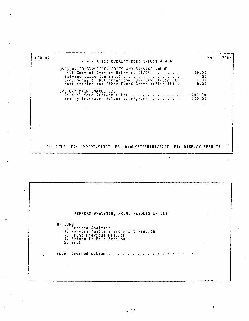
PSD-02 1 I 1 RIGID OVERLAY COST INPUTS I I t
OVERLAY CONSTRUCTION COSTS AND SALVAGE VALUE Unit Cost of Overlay Material ($/CYl •.••• Salvaoe Value (percent) •••••••.•••• Shoulders, If D1fferent than Overlay (S/lin ftl Mobilizat1on and Other Fixed Costs (S/lin ftl •
OVERLAY MAINTENANCE COST Initial Year ($/lane mile) •• , • Yearly Increase ($/lane ~ile/year) ...
80.00 20
0.00 B.OO
-700.00 100.00
No.
F11 HELP F21 IMPORT/STORE F31 ANALYZE/PRINT/EXIT F41 DISPLAY RESULTS
PERFORM ANALYSIS, PRINT RESULTS OR EXIT
OPTIONS 1. Perfor~ Analysis 2. Perform Analysis and Print Results 3. Print Previous Results 4. Return to Edit Session 5. Exit
Enter desired option •••••••••••• • • • • • •
4.13
200b

PSD-02 SOLUTION FOR INPUT DATA FILE STEVE.RR
RISID PAVEHENT STRUCTURAL DESISN
P1ve~ent Type JRCP W/ TS
Rtquired Thickness (in) 9.653
Ptrfor~ance Life (yrsl 15.0
18-kip ESAL Repetitions 17639270.
DESIGN FOR PROJECTED FUTURE OVERLAY
Overlay Type
Required Thickne5s (in)
Performance Life (yrs)
JRCP W/ TS
5.000
15.0
18-kip ESAL Repetitions 237-40120.
4.14
LIFE CYCLE COSTS (S/SYl
Initial Pavuent Construction Maintenance Salvage Value
Overlay Construction Maintenance Salvage Value
Net Present Value
-48.80 .2-4
-2. 1-4
11. 9 ~ • 13
-.69
~8.29
Press 1ny kty to continue •••

..... cu a. E C)
0 ·-0 I-<t
E ::J
~~. E ·-c ::E
p009 J!D.:J JOOd JOOd
f..J9/\
l{) ¢ r<> C\J
X9PUI Al!l!qD90fAJ9S ~U9S9Jd
4.15

"0 C)
c:
Q.)
.c
0 •
"'0 ctS 0
---------------------- co _J
Q) -
4.16

(f) o_
z (/)
-- ...... -' ' ' ' ___________ _: ~O- _ n;50_ ~n_w_
Reliability
4.17

en -ca ·-~ II Q.) w -+.J
II ca w :E Q)
0 (/)
""0 (\j 0 ..0 Q.) 0... ..0 .c ::')
""0 U) ca 0
c::
4.18

flexible Paycmentr
9.36 log10
(SN + 1) - 0.20 + logJo((4.2- Pr)/(4.2- 1.5)] 0.40 + [1094/(SN + 1)5.14]
+ 2.32 log 10~ - 8.07 1. 2.1
Rigid Pavements
log10
w18
= 7.35 log10
co + 1) - 0.06 _ logJo[(4.5- Pc)/(4.5- 1.5)]
1 + 1.624 X 10⁷
(D + 1)8.46
+ (4.22 - 0.32p )log t 10 (
o· 75
D· 75 _
- 1.132 ) 18.42
(Ec/k)"25
1.2.2
4.19

~
N 0
SUMMATION OF DAMAGE:
( 1 . 1 ) n T • (W1s) / • • • + (W1s)
12 5. 1
RIGID EQUATION
( 0 o.7s _ 1 _132 ) 3.42 w 18- i = ••• c ..•
K0.25
RELATIVE DAMAGE
1 u =
( 0 o.1s _ 1 _132 ·)3.42
K0.25
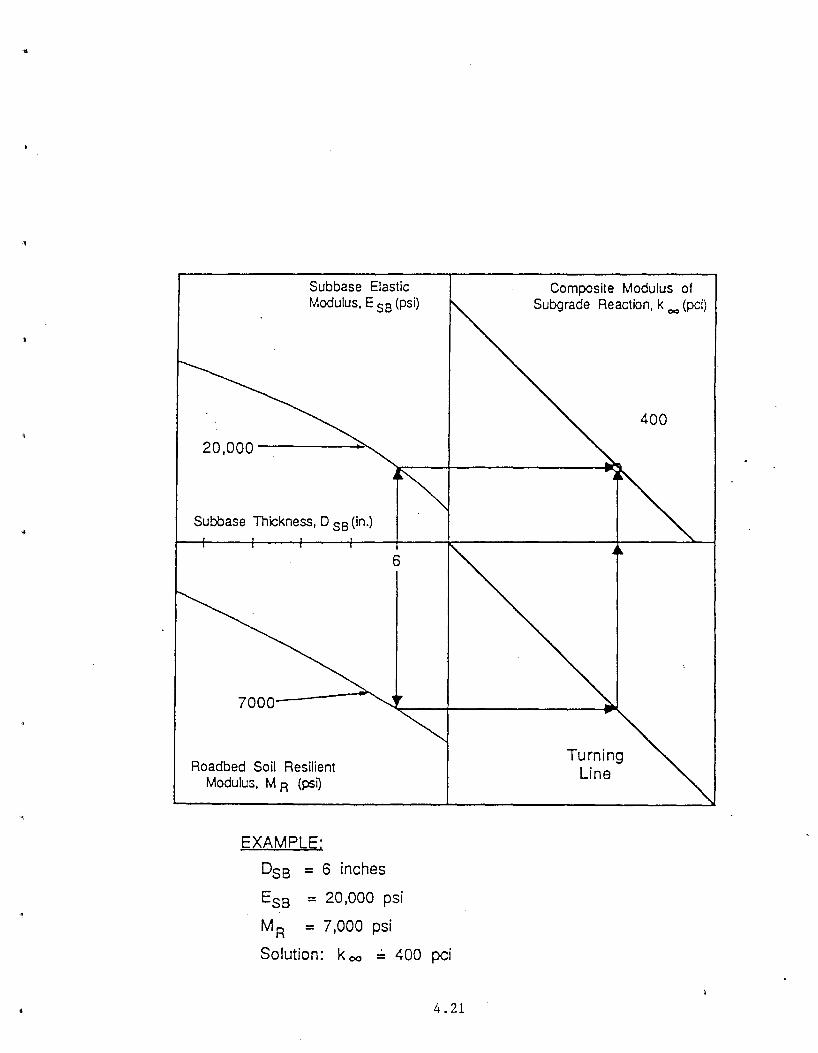
Subbase Elastic Modulus, E ss (psi)
Subbase Thickness, D ss (in.)
7000
Roadbed Soil Resilient Modulus, M R (psQ
EXAMPLE:
Dss = 6 inches
6
Ess = 20,000 psi
MR = 7,000 psi
Solution: k oo ~ 400 pci
4.21
Composite Modulus of Subgrade Reaction, k oo (pci)
Turning Line
400

-l'
N N
k1
k2
--
--
P1 = 10psi
t P2 = 10psi
+
Clay Layer
Clay Layer Rigid Layer
10 psi 200 pci -0.05 in. -
10 psi 100 pci -0.1
. -1n. Rigid Layer
• • • k Design = kchart • ( Yi) c
~ . N w
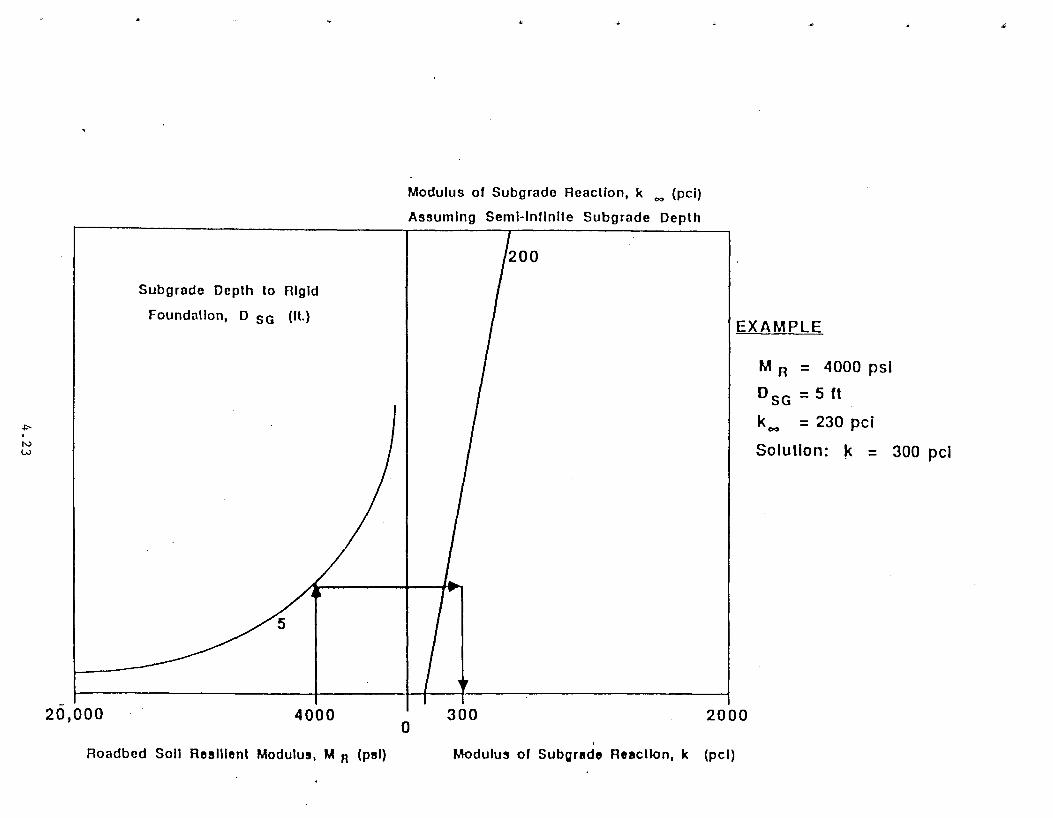
20,000
Subgrade Depth to Rigid
Foundation, D SG (ft.)
4000
Roadbed Soli Resilient Modulus, M R (psi)
Modulus of Subgrade Reaction, k oo (pel)
Assuming Semi-Infinite Subgrade Depth
EXAMPLE
M R = 4000 psi
DsG=5ft
koo = 230 pci
Solution: k = 300 pel
300 2000 0
Modulu~ of Subgrade ReacUon, k (pel)

8 10
-(/) c:: 0 -ctS (.)
0. 0. ctS
"'0 7 ctS 10 0 --
UJ EDGE WITH u.. SUPPORT LOSS -...J
r-z UJ :E 6 L!J 10 > ~ 12,000 lb. wheel load c.
. 6 E = 4.0 X 10 psi
k = 200 pci
6 7 8 9 10 11 12
SLAB THICKNESS (in.)
4.24

Chart for Considering Effect of ErodJbility
u a.
.X
§ -u 0 cv 0::
cv "0 0 '-01 .0
::::l CJ')
-0
&I)
::::l ::J
"0 Subbase 0
::E Erodability c Factor, 01 .,., cv EF a
Effective k- value ( pci)
4.25

4500 lb.
D • 3,4,5,6 1 8 and 10
inches
o2
• variable
Simulated 18-kip Single Axle Load
4500 lb.
E • 150,000 and 1 600,000 psi
E2
• 15,000 psi
v• 0.4
v• 0.35
E3
• 3,000; 7,500 v• 0.4 and 15,000 psi
Figure FF.1. Cross sections analyzed to develop relationship betYeen soil support value (Si) and roacbed soil resilient modulua (E3 or~).
4.26

..
~Crocks' -~
0 N
y
-L.
1z' ~ro'
•
r
·~
S I i t t n • u i n 1 - 0 i r • e I i o n R • d u c 1 d b y 7 5 °/o o I I h • C r o c k 1
SLAB PROPERTIES
Tnic:kneu : a" Concrete Modulus : 5 I IO' psi
Poisson's Ratio : 0.25
4 Tirts are 6000 lbs Each
CENTRAL CRACK
Void Space
#I
#2
#3
Slob Edo•
0/ 0 Area of Slob
0.00
I .59
4 .5.9
a. 16
Lou of Support Foetor
0
2
3
Figure LL.2. Slab and support conditions for erodability analysis.
4.27

Ill c..
Ill
"' 41 ... (/')
c a. <.)
c ... a.
I ' I It
300
200
100
0
9 kips 9 kips
20'
Distance Across Slob
BeQins
With Shou I d er
35'
-roo
Figure KK.l. Transverse section and stress profile for 8-inch CRCP, ~ith and ~ithout concrete shoulders. (7)
4.28

-(/)
c: 0 -ca (.) ·-c. c. ca
"C ca 0 -
w u. -fz
8 10
7 10
w 6 ~ 10 w > <X: c.
6
INTERIOR
7 8 9
12,000 lb. wheel load 6
E = 4.0 X 10 psi
k = 200 pci
10 11 12
SLAB THICKNESS (in.)
4.29
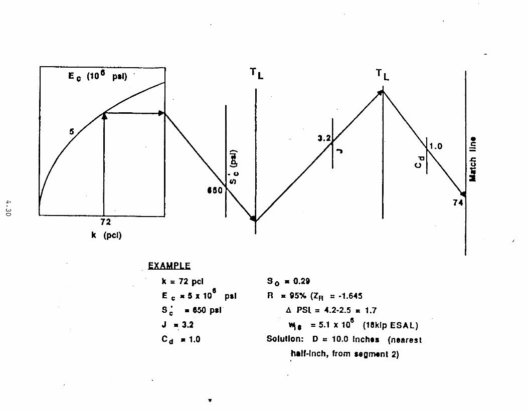
72
k (pel)
EXAMPLE;
k = 72 pel e
E c • 5 X 10 pal
s~ • 150 ,_r J • 3.2
cd • 1.0
9 0 • 0.28
A II i5% (ZA = -1.~5 11 PSL = 4.2·2.5 • 1.7
¥l\e = 5.1 X 10⁸
(18klp ESAL)
Solution: D = 10.0 Inches (nearest
half.Jnch, from segment 2)
• c --
/

CD c:
:.J
74
(J) 0.. <J
(/) (/)
0 ....J
:..0 ro Cl> (.)
-~ Cl>
(J)
c: Ol (/)
Cl> 0
Design Slab Thickness, D (inches)
Estimated Total 18-kip Equivalent Single Axle Load (ESAL) Applications, w 18 (millions)
--------------~~-------------------TL
Overall Standard Deviation, %
Reliability, R (%)
4.31

F:cs; Heave R3te. 0 (mm i day) 30
Time, t (years)
EXAMPLE
t = 15 years
0 = Smm I day
P = 30°/o
.1PSI MAX = 2.0
15
Solution: D.PSr FH = 0.47
0.47
Frost Heave Probability
Maximum Potential Serviceability Loss,
.PSI MAX
4.32
2.0

Plane
Joint Crack
Edge Steel
F5 = ~riction
!-----~~--~ ... ~X X
u •
4.33

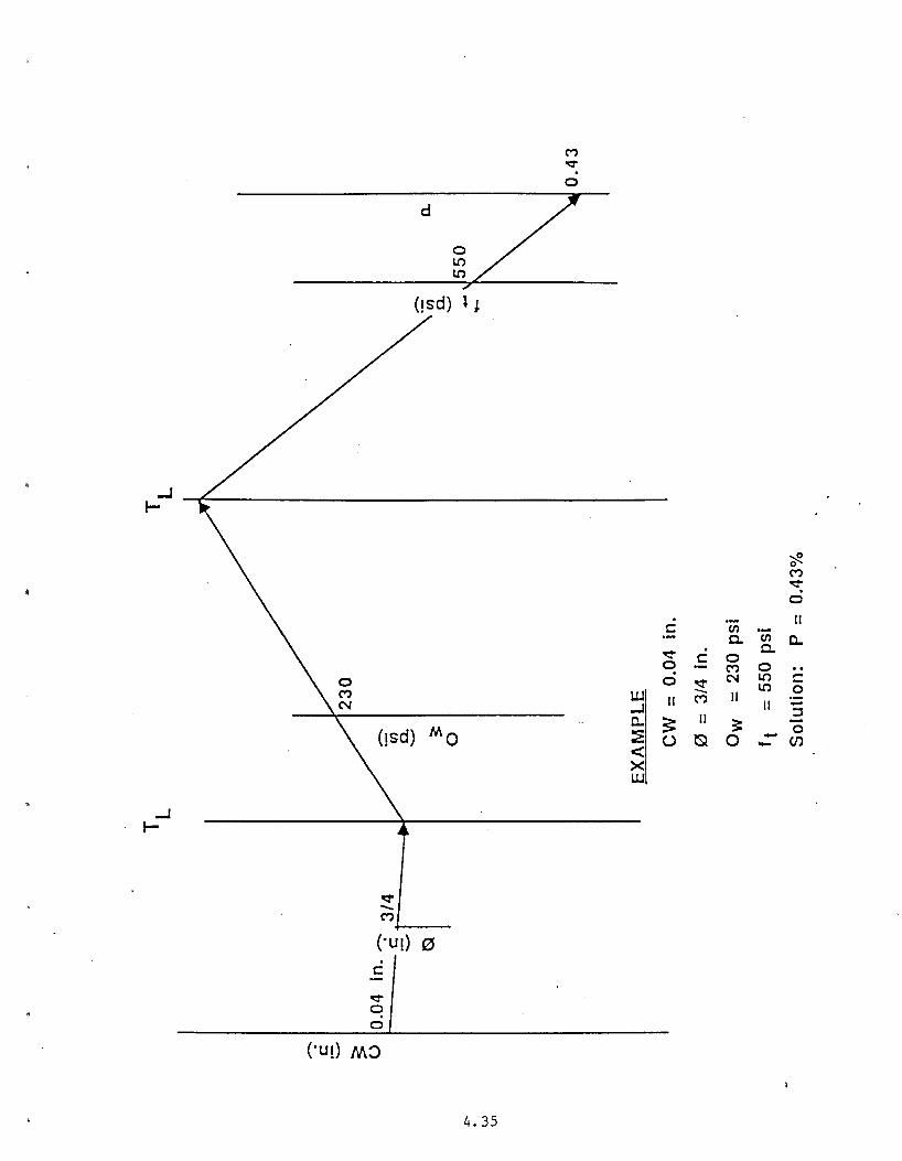
-c: -• I><
I I I I.
I I
3.5
d 1.32 -. • ~
c - &:1 c 5/8 c -
& N
..
EXAMPLE y = 3.5 ft.
ex. /rAe II: 1.3 2
0 = 518 ln.
z = 0.0004
Cfw = 230 psi
f, = 550 psi
Solution: P = 0.51%
d
(!Sd) t l
...J ....
(!Sd) Mo
..J ....
~ -M +---
('U!) M':J
4.35
M v 0
w ..J 0.. ~ < >< UJ
. c
v 0 . 0
II
$: u
~ 0 M v . 0
II (/) ·-c. (/) 0.. . c. c 0 M 0 .. N LO c
~ - LO 0 M II
II -::I II ;: 0 Q 0 - CJ) -

..J t-
0 M N
d
• 0 0 0
0
(U! I U!) z
(:lo) 0 10
,..... ~
0 u.. (/)
.X: 0 w L()
..J I"- L() L()
II II c
bCI) b
r;;( -----~------------
(!S>i) s.D
4.36
~ 0 I"-«:!' . 0
II (/)
~ c. (/) a. 0 c. 0 0 0 .. 0 M c: . N
L()
0 L() 0
II II II -::l tJ - 0
N - (/)

SESSION 5
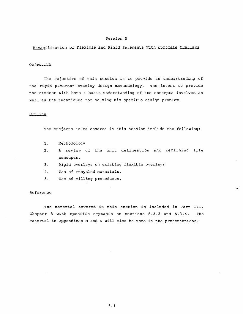
Session 5
Rehabilitation Qf Flexible ~ Rigid Pavements ~ Concrete Overlays
Objective
The objective of this session is to provide an understanding of
the rigid pavement overlay design methodology. The intent to provide
the student with both a basic understanding of the concepts involved as
well as the techniques for solving his specific design problem.
Outline
The subjects to be covered in this session include the following:
1. Methodology
2. A review of the unit delineation and remaining life
concepts.
3. Rigid overlays on existing flexible overlays.
4. Use of recycled materials.
5. Use of milling procedures.
Reference
The material covered in this section is included in Part III,
Chapter 5 with specific emphasis on sections 5. 3. 3 and 5. 3. 4. The
material in Appendices M and N will also be used in the presentations.
5. 1

~/ol
~
a-0
l AC
PCC X X
I I I I I
- - - - -:- - - --- - - --- - ---' !
AC
PCC
N
L ~T
~I
5.2
n w/ol + < 1 . . -
N w/ol
n RL = 1- w/ol
N w/ol

/11-78
c.
> ·u It)
c. ~
u
u Vl
0 u It)
u.. c
.52
~ 0 u
u
p 0
1.0
Existing Pavement
I : X
N fx
Overlaid Pavement
_\__ __
sc y
I y
scY
-I
eH
Design of Pavement Structures
lill Repe.t111onsl
~--------------~-------L----------~~----------------~-- ~
0~------------~------------------~--------~ N
1- X ... , y ~I
Figure 5.1. Relationship between serviceability-capacity condition factor and traffic.
5.3

111·82
c..
Q)
-~
"' "3 E ~
u
x=O
0
Design of Pavement Structures
.1 .. y __j ~ Traffic Repetitions
I y=O
Figure 5.3. Appropriate serviceability-traffic repetition-time curves used in traffic analysis step.
5.4

111·80
Specific overlay equ•tion form utilized.
Type Overlay Type Existing Specific Equation Conditiona/Remarb Pavement ·
Flexible Flexible SNOl. = SNY- FRLSN.uff SC=SN; n = 1.0
FlexitMe Rigid SNOl. = SNY- F RLSNuff SC a SN; n • 1.0 (IN Section 5.3.3 for specific equadons used)
Rigid Flexible D ex.= D Y (see remarks) Treat overlay anatysis as new rigid pavement destgn using existing flexibfe pavement as new foondation (aubgrade)
Rigid Rigid DOL= Oy- FRL(O~ SC = 0; .n = 1 .0 (Bonded Overlay)
o 1.4 = 0 1.4 _ F (0~1.4 SC = 0; n = 1 .4 (Partial Ol. y RL Bond Overltty)
DOL 2 = D/- FLJ!,.O._ .• ,l SC z 0; n • 2.0 (Unbonded
Overlay)
5.5

STEP 1 STEP 4
Analysis Unit ... Effective Structural Delineation
-,.. Capacity Analysis
scxeff
, r STEP 2 STEP 5 STEP 7
Traffic Future Overlay
Overlay Design Analysis Structural Capacity .. .... Analysis Analysis
scy
, r
STEP 3 STEP 6 Materials and Remaining Life
Environmental Study Factor Determination
FRL
Figure 2.5. Required overlay des~gn steps.
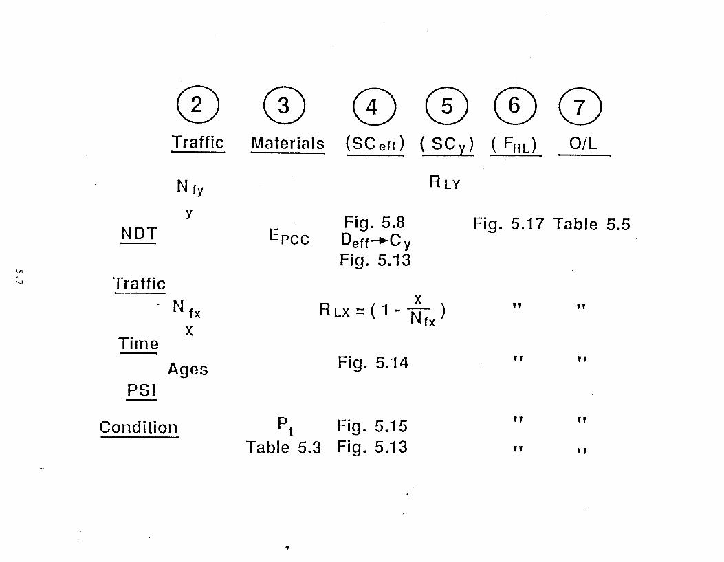
0 0 CD 0 ® (j) Traffic Materials (SCetr) ( SCy) ( FRL) 0/L
N ty RLv
y Fig. 5.8 Fig. 5.17 Table 5.5
NOT Epee Dett-+C y
Fig. 5.13 Vt .
Traffic -.....)
· N fx X
" " R LX= ( 1-- ) Nrx
X Time
Fig. 5.14 " " Ages PSI
Condition pt Fig. 5.15 " " Table 5.3 Fig. 5.13 " "

/11·91 Design of Pavement Structures
00=16.0"
"' Gl
-5 :§.
"' "' c:> c: 0
0 = 8.0" j/;
.!:? 8 ;: c c:> E c:> > <a
c.. u 6 u c.. Gl
.2: u ~ w
4
"i .. c
2
1.0 2.0 3.0 4.0 5.0 6.0
EPCC · In Situ PCC Modulus from NOT (psi x 106 l
Figure 5.8. Determination of effective PCC structural capacity (thickness) from NOT-derived PCC
modulus.
5.8

/11·100
j a:
De:sig11 of Pavement Stn.Jcture:s
100
0 ·.5 .6 .7 .8 .9 1.0
Cx · Pavement Condition Factor
Figure 5. 13. Remaining life estimate predicted from pavement condition factor.
5.9

I Rehabilitation Methods wit It Overlays 111·101
.. 100 0 v g
75 T 25 g
50 50
25 75
100 100
* ~ 75 vg = Q) .2! Cl <::)
T, 25 :J E
<::) Cl
0 . -~ 50
c: c.; 50 CD
E E Q) ~
> c: <::) 25 75 c..
~
" E
"'0 ~
100 100 > "' c..
75 I 25 X
..J c:
50 50
25 75
0 10 !5 20 Z?
t · Time To Overlay (years)
Figure 5. 14. Remaining life estimate based on time considerations for various traffic growth rates.
5.10

/ll·/02 Desigra of Pavemerat Strucrures
75
50
50
25 Flexible Pavements
0 2.0 2.5 3.0 3.5 4.0 4.5
P 11 Serviceability at Time of Overlay
Figure 5. 15. Remaining life estimate based on present serviceability value and pavement cross section.
5.11

Rehabilitation Methods with Overlays
Table 5.3. Summary of visual (C) and structural (C) condition valuec.
uyer Type
Asphaltic
PCC
Pozzolanic Base/ Subbase
Granular Base/ Subbase
Special Notes:
Pavement Condition
1. Asphalt layers that are sound, stable, uncradted and have little to no deformation in the wheel paths
2. Asphalt layers that exhibit some intermittent cracking w1th slight to moderate wheel path deformauon but are still stable.
3. Asphalt layers that exhibit some moderate to high cracking, have ravelling or aggregate de9radat1on and show moderate to high deformations 1n wheel path
4. Asphalt layers that show very heavy (extensive) cracking, considerable ravelling or de9radation and very appre<:1able wheel path deformations
1. PCC pavement that is uncracked, stable and undersealed, exhibiting no ev1dence of pumping
2. PCC pavement ·that is stable and undersealed but shows some imtial cracking (with tight, non working cracks) and no evidence of pump.ng
3. PCC pavement that is appreciably cracked or faulted with signs of progressive crack deterioration: slab fragments may range in size from I to 4 sq.yds., pumping may be present
4. PCC pavement that is very badly cracked or shattered intoJragments 2-3 ft. in maximum size
1. Chemically stabilized bases '(CTB. LCF ... ) that are relatively crack free, stable and show no evidence of pumping
2. Chemically stabilized bases (CTB. LCF ... ) that have developed very strong panern or fatigue cracking, with wide and working cracks that are progressive in nature: evidence of pumping or other causes of instability may be present
t. Unbound granular layers showing no evidence of shear or densification distress, reasonably identical physical propenies as when constructed and existing at the same "normal" moisture· density conditions as when constructed
2. Visible evidence of significant distress within layers (shear or densification), aggregate propenies have changed significantly due to abrasion, intrusion of fines from subgrade or pumping, and/or significant change in in situ moisture caused by surface infiltration or other sources
I. The visual condition factor. c.,. is related to the structural condition factor, c.- by:
c ,. c 2 • •
C Viaual Condition F~Of !'an~
0.9·1.0
0.7-0.9
0.5-0.7
0.3·0.5
0.9-1.0
0.7-0.9
0.5-0.7
0.3-0.5
0.9-1.0
0.3-0.5
0.9-1.0
0.3-0.5
11/·103
Cli.Struct Cond Factor Valua
.95
.85
.70
.60
.95
.85
.70
.60
.95
.60
.95
.60
2. The structural condition factor. Cx:' and not the c. value, is the variable used in ths structural overlay design equation (for all overlay-ex1stmg pavement types). It 11 defined by:
5.12

lll·/06
.. 0 u Ill
1.1.
..J a:
1.1.
.9 .9
.8 .8
.7 .7
.6 .6
.5 .5
.4 ~_.--~--~~--~_.--~~--~--~_.--~_.--~~--~~~~--~~ .4 100 60 40 20 0
RLv A.emaining Life (Overlaid Pavement) ~
Figure 5.17. Remaining life factor as a function of remaining life of existing and overlaid pavements.
5.13

lll·/08 Design of Pavement Structures
Table 5.5. Summary of overlay equations used in flexible overlay over existing rigid pavement analyaia.
Major Overlay Condition
Normal Structural Overlay
Break-Seat Overlay
Specific Method Used
NOT Method 1
NOT Method 2
Visual Condition Factor
Estimating Nominal Crack Spacing
Post Cracking NOT
(a)NOT Method 1
(b) NOT Method 2
SN oiEquation
SNol = SNY. F RL(0.8 0 uff + SNxeff-rJ
SNol = SNY· FRLSNxeff
SNol = SNY. FRL( a2roo + SNxeff-rp
SN 01 =SNv·0.7(abcOo +SNx.tt-rJ
SNol = SNY • 0.7 SNxeff
Special Note: The coefficient of 0 {ie.,0.4) actually varies from 0.35 for a nominal craclc spacing of approximately 2.0 ft. to a value of 0.45 for a nominal crack spacing of approximately 3.0 ft.
5.14

Rehabilitation Methods with Overlays
Table 5.6. Minimum asphalt concrete structural overlay thick.neu for PCC Pavements (from the Asphatt Institute MS-1 7).
Existing h (.min - incha)
Maximum Annua Temperature Differential (I>J:) PCC Slab Length (ft) 30 40- 50 80 70 80
10 4 4 4 4 4 4 15 4 4 4 4 4 4 20 4 4 4 4 5 5.5 25 4 4 4 5 6 7 30 4 4 5 6 7 8 35 4 4.5 6 7 8.5 • 40 4 5.5 7 8 • • 45 4.6 6 7.5 9 • • 50 5 7 8.5 • • • 60 6 8 • • • •
• Alternate other than thickness of AC overlay should definitely be considered to minimize reflective cracking.
5.15
11/·109

•·
..
lll-!12 Desig" of PavemeM Stn.~ctures
Table 5.8. Summary of concrete overlays on exist!ng concrete pavements.
TYPE OF OVERLAY
PROCEDURE
MATCHING OF' }LOCATION JOINTS IN OVER-LAY e PAVEMENT TYPE
REfLECTION OF' UNDERLYING CRACKS
TO BE EXPECTED
UNBONOCD OR S(P.l~ATEO PARTIALLY 80N0(0 OA OV(RLAY OIR~CT OV!RLAY
CL.(AN SUIH'AC( 0(11'11$ CL.(AH $UI'IF1Ct O(II'IIS AND (XCtsS JOINT S(AL. AHO (XC(SS JOINT S(AL. PL..IJ:( S(PAIU.TION COUIIIS(- ANO l'l(looiOV( (XC(SSIV( 01\.. I"L.AC( OV(IIII...lr CONCI'I(T(. AHO I'IUII(I'I.- I'I..AC( OV£111-
NOT NECESSARY
NOT NECESSARY
NOT NORI.IALLY
I..AY CONCIII(T(
REQUIRED
NOT NECESSARY
USUALLY
REQUIREMENT FOR STEEL REINFORCE
MENT
I A(OUIIIIE,Iol(l'cT IS INO(.P(NO(NT III(OUIIII(Ioi(NT IS INO(I'(HOCHT or TM( ST(E.l. D( (XISTINC OF TM( STt(L, IN (XISTIHC
'" SMOUI..O IE lASCO ON I Tto~( I'L.(X~AL STR(NGTH OF
MINIMUM THICKNESS I 1- NO STRuCTU-
~ .._ ~ AAI.. Otf'E.CTS
I'AV(W(NT 0111 C:ONOITIOH Pt.V(W(._T, ST((L. loiAT I(
OF EXISTING PAV(W(NT.
6"
YCS
USE.O TO CONTROl.. C:R.I.CKINC WHICH loiAT II£ C.:.US~ liT
l.IWITEO )ION-STIIIuCTUIIIAl. O(I"(CTS IN •t.v( W(NT,
Ovt:IIII..AT C:ONCRnt
YES
BONDED OR WONOLITHIC OVERLAY
SCAI'III'Y Al..l. 1..005( COHCI'I(T(,CI..(AH .OINTS,C:L.(AN AHO ACID [ TCH SUIIIFAC'! -,...,_AC( IOHOIHC CIIIOUT I-NO OV(RI..AY CONCI'I(T£.
REOUIREO
REQUIRED
YES
NOIIIIoiAl.LY NOT US(O IN THIN OV[IIIl.AYS.IN THICK(A OV(JIIti..AT STt£1. WAT IE
US£0 TO SUPPL.(W(NT STE:EL IN (liSTING Pt.V(Ioi(.HT.
(XISTING COf'oiCR(T(
I"
YE:S 0. ~0: C I 1,0 O
~ g~.., I..IW.IT(O STR• YES OHI..T " 0(f'£CTS CAN II( ONl.T II' Otf'CCTS' CAN II( ,_ ,....- z_ UCT. O(F(CTS
1.1.. >- v _ ,_ .._ ~~C:-;';-;-0.:.;. 7~~:-;·;-:-t------------r-"-t_P_A-III_E:_O:__ ______ +_".:.E_I'_t.I:.:.I'I.:.:E::0~-------4
>- _J o-0 "'"" VCT DEFECTS YE:S NO NO
0 <=: ~~ ~z 1 SEVERE STA- I a:: .,..,,..;t: C•O.~~·
~ WFT~~========~==================~==================~==================~ -J_- 0> ~I,:,-
v..J z YE.S YE:S
~ U) ~! ~ ~ t------t------------1------------+-------------l N(GI..IGIIII..( YES
u;::) v.,..,.., I i ~ g~ ~a l--1.-1 .. _1 T_E_o_-+------Y-E_s ____ --f-----Y-E_S-----+-----Y_E_S-------l Cl. < q:~"~ < > ~ ... ! ... (XT(HSIV( YES NO YES
• C VAI..U(S A"I'I..T TO STI'IUCTV"AI.. COHOITION OICI..T,
.&.1110 SMOU\..0 HOT I( INI"UJE.HC£0 IY SUI'I,.AC( O(I'(CTS,
5.16

SESSION 6

Session 6
Implementation Guidelines
Objective
The primary objective of this session is
attendees to implement the Guides and provide
to encourage the
basic procedural
guidelines for an agency to implement the new concepts. Illustrative
examples of the procedures that may be used by the States will be
provided.
Outline
This session will be primarily covered by a slide show. The
primary topics to be covered as to implementation are as follows:
1. The basic problems will be defined.
2. The agency needs will be outlined.
3. The alternate approaches or solutions will be covered.
4. A basic sample plan will be formulated to illustrate the
concepts involved.
5. The need for implementation will be emphasized.
After the session closes, the student will be asked to complete
and submit the training course evaluation form.
Reference
The reading assignment for supporting the information provided in
this session will be the Preface and Executive Summary of the Guide.
6.1

PROBLEM
NEEDS
ALTERNATE SOLUTIONS
FORMULATE A PLAN
IMPLEMENT
6.2

Improvements to the Guide
" 1 . RELIABILITY
2. MR FOR SOILS 3. M· R FOR LAYER COEFFICIENTS
4. DRAINAGE
5. ENVIRONMENT
6. LOAD POSITION
7. SUBBASE EROSION
8. LIFE CYCLE COSTS
9. REHABILITATION
1 0. PAVEMENT MANAGEMENT
11 . LOAD EQUIVALENCIES
12. TRAFFIC DATA
13. LOW VOLUME ROADS
14. MECHANISTIC I EMPIRICAL DESIGN·
6.3

SENSITIVITY STUDY
• Select panel
• Select range for each variable
• Solve for thickness (D)
• Plot graph of "D" vs. Variable range
• Prioritize in decreasing order of sensitivity
• Assess current knowledge
• Development program
Alter charts as needed
Characterization of variables
Commit resources on basis of priority I need
6.4

- .r: - C) - ·-- Q) J: - -.0 .UJ
Q) ca ::> . -.0 lo..
...J ca ca lo.. > E <( ca
/ > > ::J ·-"C Q)
UJ :: > -t-<( ...J
;: UJ 0 c: ...J
SS3N)f81Hl !N311\13AV'd
6.5

PSI
STATE LOW HIGH
A 550 650 1000
11 •
c ·-"" 10 en
en LU z
9 ~ 0 -:r:
0'\ l-0'\ 8
l-z LU :E 7 LU > <t a..
Low Medium High
RELATIVE CONCRETE STRENGTH

0 Lf) ..J
LU >
0') LU 0') ..J
>-1-..J -c::l ~ ..J LU a: ~ 0 0
oc 1..0
1-0 1-:::r::::r: ~ Cl)l-~LU ~:E Cl
Sl3A31 Al.lli8V'll3H SnOIH\f A l. \f - Q
6.7

0 1{)
0) 0)
w Cl :::>
" 0 1-J: (./)
c:::x: c:::x:
Cl
3GinD WIH3.LNI - 0
6.8

FUNCTIONAL RECOMMENDED LEVEL OF RELIABILITY
CLASSIFICATION URBAN RURAL
INTERSTATE, 85 - 99.9 80 - 99.9 FREEWAYS
PRINCIPAL 00 - 99 75 - 95 ARTERIES
COLLECTORS 80 - 95 75 - 95
LOCAL 50 - 80 50 - 80

CJ) :;::) ..J :;::)
zO -o UJ:E (.!) ZUJ <tO ::I:<t ua:
(.!)
c:J :;::) CJ)
NQfj_831.:130
6.10
c: w cc ~ ::> z cr: 0 (f) z w (f)

X
.X
-en c.
-u.. u.. < c: 1-
6.11

0
~ ~ z <1 0 -
" w a:
0 <1
NOI1~31::130
6.12
Ci3 u.
\,.
a> E E ::I
U)
UJ ~ 1-

CD
z 0 (!J UJ
~
0
< z 0
~
-C/) a.
6. 13
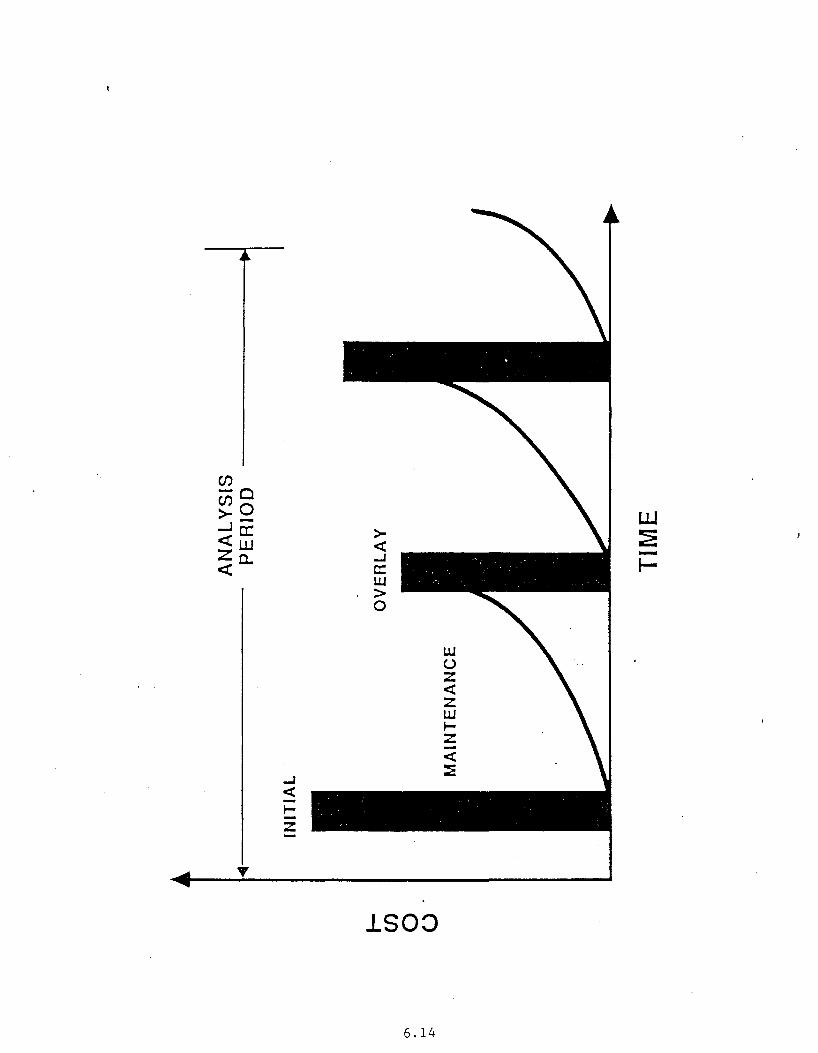
Cf) -o cno >-_ ...Ja: <t:w Za. <t:
...J < .... -z
>< ...J a: w > 0
lSOO
6.14
w (.) z < z w .... z < ::
-

("")
Cl 0
C\1 1-Cl z
UJ 1-
or- z Cl 0
(.)
~ UJ 0: ~
or- >< 1-Cl II CJ) A -0 C\1
Cl 2 A
Cl("")
NOI1~31.:130
6.15

en ,.... N c c en
>- c: 0 0 X
-I
1-<!
(.)
z <!
<l: u.
z 0 E
X 1-
en 0
z en
UJ w
~
1-0:
II
" z w 0: en z ,
0 (.)
,.... UJ c c: A ::::> N 1-c (./') -0
~
6.16

Name (optional)
Job Responsibility
AASHTO PAVEMENT DESIGN ~ORKSHOP
TRAINING COURSE EVALUATION FORM
Date
Instructions: Please complete the following questionnaire. Your
responses will provide valuable feedback and will assist in planning
subsequent course presentations.
Several items will be rated on a scale ranging from 1 to 7 and defined as
follows:
1. Poor
2. ~ell below average
3. Below average
4. Average (acceptable)
5. Good
6. Ve::y good
7. Excellent
Please circle the number which reflects your rating.
1. Please rate the course on its overall value and significance to you.
1 2 3 4 5 6 7
Comments
2. ~ere the stated objectives of the course achieved?
Very well Reasonably well
3. The le~gth of the course was:
Much too long
Short
Too long
Very short
No
About right

4. Should addition topics be covered, or should some topics be reduced or
eliminated?
Comments
5. For the intended participant, the level of technical content was:
extremely detailed
somewhat detailed
about right
somewhat general
extremely general
Comments
6. Please rate the visual aids. Poor Average Excellent
1 2 3 4 5 6 7
7. ~ould you recommend this course to your fellow workers?
~y or why not?
8. ~at constructive suggestions would you offer for improvement of
future presentations of this course?