Embed Size (px)
Citation preview
Cellarosi, F., & Marklof, J. (2016). Quadratic Weyl sums, automorphicfunctions, and invariance principles. Proceedings of the LondonMathematical Society, 113(6), 775–828.https://doi.org/10.1112/plms/pdw038
Peer reviewed version
Link to published version (if available):10.1112/plms/pdw038
Link to publication record in Explore Bristol ResearchPDF-document
This is the accepted author manuscript (AAM). The final published version (version of record) is available onlinevia London Mathematical Society at http://doi.org/10.1112/plms/pdw038. Please refer to any applicable terms ofuse of the publisher.
University of Bristol - Explore Bristol ResearchGeneral rights
This document is made available in accordance with publisher policies. Please cite only thepublished version using the reference above. Full terms of use are available:http://www.bristol.ac.uk/red/research-policy/pure/user-guides/ebr-terms/
Quadratic Weyl Sums, Automorphic Functions,
and Invariance Principles
Francesco Cellarosi∗, Jens Marklof†
June 27, 2016
Abstract
Hardy and Littlewood’s approximate functional equation for quadratic Weyl
sums (theta sums) provides, by iterative application, a powerful tool for the asymp-
totic analysis of such sums. The classical Jacobi theta function, on the other hand,
satisfies an exact functional equation, and extends to an automorphic function on
the Jacobi group. In the present study we construct a related, almost everywhere
non-differentiable automorphic function, which approximates quadratic Weyl sums
up to an error of order one, uniformly in the summation range. This not only im-
plies the approximate functional equation, but allows us to replace Hardy and
Littlewood’s renormalization approach by the dynamics of a certain homogeneous
flow. The great advantage of this construction is that the approximation is global,
i.e., there is no need to keep track of the error terms accumulating in an iterative
procedure. Our main application is a new functional limit theorem, or invariance
principle, for theta sums. The interesting observation here is that the paths of
the limiting process share a number of key features with Brownian motion (scale
invariance, invariance under time inversion, non-differentiability), although time
increments are not independent and the value distribution at each fixed time is
distinctly different from a normal distribution.
∗Queen’s University. 506 Jeffery Hall, University Avenue. Kingston, ON K7L 3N6. Canada,
[email protected]†School of Mathematics, University of Bristol, Bristol BS8 1TW, U.K., [email protected]
1
Contents
1 Introduction 3
2 Jacobi theta functions 12
2.1 The Heisenberg group and its Schrodinger representation . . . . . . . . . 12
2.2 Definition of SL(2,R) . . . . . . . . . . . . . . . . . . . . . . . . . . . . . 13
2.3 Shale-Weil representation of SL(2,R) . . . . . . . . . . . . . . . . . . . . 14
2.4 The Jacobi group and its Schrodinger-Weil representation . . . . . . . . . 15
2.5 Geodesic and horocycle flows on G . . . . . . . . . . . . . . . . . . . . . 16
2.6 Jacobi theta functions as functions on G . . . . . . . . . . . . . . . . . . 16
2.7 Transformation formulæ . . . . . . . . . . . . . . . . . . . . . . . . . . . 17
2.8 Growth in the cusp . . . . . . . . . . . . . . . . . . . . . . . . . . . . . . 19
2.9 Square integrability of Θf for f ∈ L2(R). . . . . . . . . . . . . . . . . . . 21
2.10 Hermite expansion for fφ . . . . . . . . . . . . . . . . . . . . . . . . . . . 21
2.11 The proof of Theorem 1.1 . . . . . . . . . . . . . . . . . . . . . . . . . . 24
3 The automorphic function Θχ 26
3.1 Dyadic decomposition for Θχ . . . . . . . . . . . . . . . . . . . . . . . . 27
3.2 Hermite expansion for ∆φ . . . . . . . . . . . . . . . . . . . . . . . . . . 32
3.3 Divergent orbits and Diophantine conditions . . . . . . . . . . . . . . . . 33
3.4 Proof of Theorem 1.2 . . . . . . . . . . . . . . . . . . . . . . . . . . . . . 36
3.5 Hardy and Littlewood’s approximate functional equation . . . . . . . . . 41
3.6 Tail asymptotic for Θχ . . . . . . . . . . . . . . . . . . . . . . . . . . . . 42
3.7 Uniform tail bound for Θχ . . . . . . . . . . . . . . . . . . . . . . . . . . 47
4 Limit theorems 50
4.1 Equidistribution theorems . . . . . . . . . . . . . . . . . . . . . . . . . . 50
4.2 Convergence of finite-dimensional distributions . . . . . . . . . . . . . . . 52
4.3 Tightness . . . . . . . . . . . . . . . . . . . . . . . . . . . . . . . . . . . 56
4.4 The limiting process . . . . . . . . . . . . . . . . . . . . . . . . . . . . . 58
4.5 Invariance properties . . . . . . . . . . . . . . . . . . . . . . . . . . . . . 60
4.6 Continuity properties . . . . . . . . . . . . . . . . . . . . . . . . . . . . . 62
References 65
2
1 Introduction
In their classic 1914 paper [22], Hardy and Littlewood investigate exponential sums
of the form
SN(x, α) =N∑n=1
e(
12n2x+ nα
), (1.1)
where N is a positive integer, x and α are real, and e(x) := e2πix. In today’s literature
these sums are commonly refered to as quadratic Weyl sums, finite theta series or theta
sums. Hardy and Littlewood estimate the size of |SN(x, α)| in terms of the continued
fraction expansion of x. At the heart of their argument is the approximate functional
equation, valid for 0 < x < 2, 0 ≤ α ≤ 1,
SN(x, α) =
√i
xe
(−α
2
2x
)SbxNc
(− 1
x,α
x
)+O
(1√x
), (1.2)
stated here in the slightly more general form due to Mordell [38]. This reduces the length
of the sum from N to the smaller N ′ = bxNc, the integer part of xN (note that we may
always assume that 0 < x ≤ 1, replacing SN(x, α) with its complex conjugate if nec-
essary). Asymptotic expansions of SN(x, α) are thus obtained by iterating (1.2), where
after each application the new x′ is −1/x mod 2. The challenge in this renormalization
approach is to keep track of the error terms that accumulate after each step, cf. Berry
and Goldberg [2], Coutsias and Kazarinoff [11] and Fedotov and Klopp [16]. The best
asymptotic expansion of SN(x, α) we are aware of is due to Fiedler, Jurkat and Korner
[17], who avoid (1.2) and the above inductive argument by directly estimating SN(x, α)
for x near a rational point.
Hardy and Littlewood motivate (1.2) by the exact functional equation for Jacobi’s
elliptic theta functions
ϑ(z, α) =∑n∈Z
e(
12n2z + nα
), (1.3)
where z is in the complex upper half-plane H = {z ∈ C : Im z > 0}, and α ∈ C. In this
case
ϑ(z, α) =
√i
ze
(−α
2
2z
)ϑ
(− 1
z,α
z
). (1.4)
The theta function ϑ(z, α) is a Jacobi form of half-integral weight, and can thus be
identified with an automorphic function on the Jacobi group G which is invariant under
a certain discrete subgroup Γ, the theta group. (Formula (1.4) corresponds to one of the
generators of Γ.) In the present study, we develop a unified geometric approach to both
functional equations, exact and approximate. The plan is to construct an automorphic
function Θ : Γ\G → C that yields SN(x, α) for all x and α, up to a uniformly bounded
error. This in turn enables us not only to re-derive (1.2), but to furthermore obtain an
asymptotic expansion without the need for an inductive argument. The value of SN(x, α)
3
for large N is simply obtained by evaluating Θ along an orbit of a certain homogeneous
flow at large times. (This flow is an extension of the geodesic flow on the modular
surface.) As an application of our geometric approach we present a new functional limit
theorem, or invariance principle, for SN(x, α) for random x.
To explain the principal ideas and results of our investigation, define the generalized
theta sum
SN(x, α; f) =∑n∈Z
f( nN
)e(
12n2x+ nα
), (1.5)
where f : R → R is bounded and of sufficient decay at ±∞ so that (1.5) is absolutely
convergent. Thus SN(x, α) = SN(x, α; f) if f is the indicator function of (0, 1], and
ϑ(z, α) = SN(x, α; f) if f(t) = e−πt2
and y = N−2. (We assume here, for the sake of
argument, that α is real. Complex α can also be used, but lead to a shift in the argument
of f by the imaginary part of α, cf. Section 2.)
A key role in our analysis is played by the one- resp. two-parameter subgroups {Φs :
s ∈ R} < G and H+ = {n+(x, α) : (x, α) ∈ R2} < G. The dynamical interpretation of
H+ under the action of Φs (s > 0) is that of an unstable horospherical subgroup, since
(as we will show)
H+ = {g ∈ G : ΦsgΦ−s → e for s→∞}. (1.6)
(Here e ∈ G denotes the identity element.) The corresponding stable horospherical
subgroup is defined by
H− = {g ∈ G : Φ−sgΦs → e for s→∞}. (1.7)
There is a completely explicit description of these groups, which we will defer to later
sections.
The following two theorems describe the connection between theta sums and auto-
morphic functions on Γ\G. The proof of Theorem 1.1 (for smooth cut-off functions f)
follows the strategy of [32]. Theorem 1.2 below extends this to non-smooth cut-offs by
a geometric regularization, and is the first main result of this paper.
Theorem 1.1. Let f : R → R be of Schwartz class. Then there is a square-integrable,
infinitely differentiable function Θf : Γ\G → C and a continuous function Ef : H− →[0,∞) with Ef (e) = 0, such that for all s ∈ [0,∞), x, α ∈ R and h ∈ H−,∣∣SN(x, α; f)− es/4 Θf (Γn+(x, α)hΦs)
∣∣ ≤ Ef (h), (1.8)
where N = es/2.
Of special interest is the choice h = e, since then SN(x, α; f) = es/4 Θf (Γn(x, α)Φs).
As we will see, Theorem 1.1 holds for a more general class of functions, e.g., for C1
functions with compact support (in which case Θf is continuous but no longer smooth).
For more singular functions, such as piecewise constant, the situation is more complicated
4
and we can only approximate SN(x, α) for almost every h. We will make the assumptions
on h explicit in terms of natural Diophantine conditions, which exclude in particular
h = e.
Theorem 1.2. Let χ be the indicator function of the open interval (0, 1). Then there is
a square-integrable function Θχ : Γ\G→ C and, for every x ∈ R, a measurable function
Exχ : H− → [0,∞) and a set P x ⊂ H− of full measure, such that for all s ∈ [0,∞),
x, α ∈ R and h ∈ P x, ∣∣SN(x, α)− es/4 Θχ(Γn+(x, α)hΦs)∣∣ ≤ Ex
χ(h), (1.9)
where N = bes/2c.
This theorem in particular implies the approximate functional equation (1.2), see
Section 3.5.
The central part of our analysis is to understand the continuity properties of Θχ and
its growth in the cusps of Γ\G, which, together with well known results on the dynamics
of the flow Γ\G → Γ\G, Γg 7→ ΓgΦs, can be used to obtain both classical and new
results on the value distribution of SN(x, α) for large N . The main new application
that we will focus on is an invariance principle for SN(x, α) at random argument. A
natural setting would be to take x ∈ [0, 2], α ∈ [0, 1] uniformly distributed according to
Lebesgue measure. We will in fact study a more general setting where α is fixed, and12n2 is replaced by an arbitrary quadratic polynomial P (n) = 1
2n2 + c1n + c0, with real
coeffcients c0, c1. The resulting theta sum
SN(x) = SN(x;P, α) =N∑n=1
e (P (n)x+ αn) , (1.10)
is not necessarily periodic in x. We thus assume in the following that x is distributed
according to a given Borel probability measure λ on R which is absolutely continuous
with respect to Lebesgue measure.
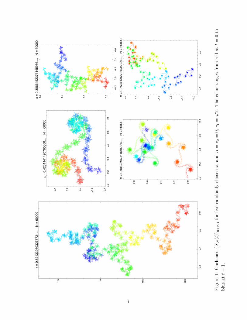
Let us consider the complex-valued curve [0, 1]→ C defined by
t 7→ XN(t) =1√NSbtNc(x) +
{tN}√N
(SbtNc+1(x)− SbtNc(x)). (1.11)
Figure 1 shows examples of XN(t) for five randomly generated values of x.
Consider the space C0 = C0([0, 1],C) of complex-valued, continuous functions on [0, 1],
taking value 0 at 0. Let us equip C0 with the uniform topology, i.e. the topology induced
by the metric d(f, g) := ‖f − g‖, where ‖f‖ = supt∈[0,1] |f(t)|. The space (C0, d) is
separable and complete (hence Polish) and is called the classical Wiener space. The
probability measure λ on R induces, for every N , a probability measure on the space C0
of random curves t 7→ XN(t). For fixed t ∈ [0, 1], XN(t) is a random variable on C. The
second principal result of this paper is the following.
5
-0.6
-0.4
-0.2
0.0
0.0
0.5
1.0
1.5
x=0.821339303278721...,
N=60000
0.0
0.2
0.4
0.6
0.8
1.0
-0.4
-0.2
0.0
0.2
0.4
x=0.4201141490785808...,N
=60000
-0.2
0.0
0.2
0.4
0.6
0.0
0.5
1.0
1.5
x=0.3866452376145986...,N
=60000
0.0
0.2
0.4
0.6
0.8
0.0
0.2
0.4
0.6
0.8
x=0.9062394051094856...,N
=60000
-0.4
-0.2
0.0
0.2
-1.0
-0.8
-0.6
-0.4
-0.2
0.0
0.2x=0.7504136536635329...,N
=60000
Fig
ure
1:C
url
icues{X
N(t
)}0<t≤
1fo
rfive
random
lych
osen
x,
andα
=c 0
=0,c 1
=√
2.T
he
colo
rra
nge
sfr
omre
datt
=0
to
blu
eatt
=1.
6
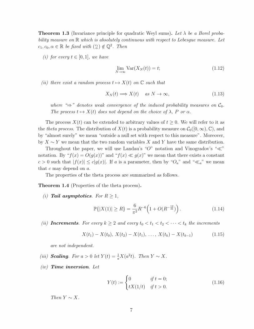
Theorem 1.3 (Invariance principle for quadratic Weyl sums). Let λ be a Borel proba-
bility measure on R which is absolutely continuous with respect to Lebesgue measure. Let
c1, c0, α ∈ R be fixed with (c1α ) /∈ Q2. Then .
(i) for every t ∈ [0, 1], we have
limN→∞
Var(XN(t)) = t; (1.12)
(ii) there exist a random process t 7→ X(t) on C such that
XN(t) =⇒ X(t) as N →∞, (1.13)
where “⇒” denotes weak convergence of the induced probability measures on C0.
The process t 7→ X(t) does not depend on the choice of λ, P or α.
The process X(t) can be extended to arbitrary values of t ≥ 0. We will refer to it as
the theta process. The distribution of X(t) is a probability measure on C0([0,∞),C), and
by “almost surely” we mean “outside a null set with respect to this measure”. Moreover,
by X ∼ Y we mean that the two random variables X and Y have the same distribution.
Throughout the paper, we will use Landau’s “O” notation and Vinogradov’s “�”
notation. By “f(x) = O(g(x))” and “f(x)� g(x)” we mean that there exists a constant
c > 0 such that |f(x)| ≤ c|g(x)|. If a is a parameter, then by “Oa” and “�a” we mean
that c may depend on a.
The properties of the theta process are summarized as follows.
Theorem 1.4 (Properties of the theta process). .
(i) Tail asymptotics. For R ≥ 1,
P{|X(1)| ≥ R} =6
π2R−6
(1 +O(R−
1231 )). (1.14)
(ii) Increments. For every k ≥ 2 and every t0 < t1 < t2 < · · · < tk the increments
X(t1)−X(t0), X(t2)−X(t1), . . . , X(tk)−X(tk−1) (1.15)
are not independent.
(iii) Scaling. For a > 0 let Y (t) = 1aX(a2t). Then Y ∼ X.
(iv) Time inversion. Let
Y (t) :=
{0 if t = 0;
tX(1/t) if t > 0.(1.16)
Then Y ∼ X.
7
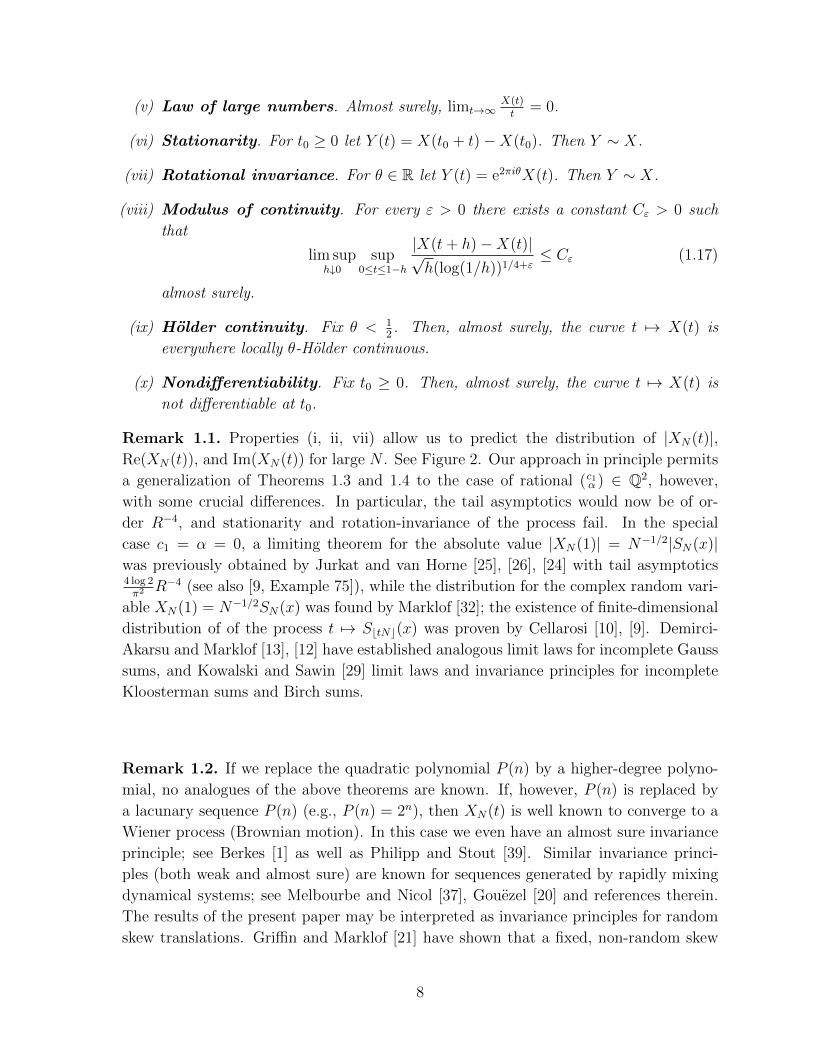
(v) Law of large numbers. Almost surely, limt→∞X(t)t
= 0.
(vi) Stationarity. For t0 ≥ 0 let Y (t) = X(t0 + t)−X(t0). Then Y ∼ X.
(vii) Rotational invariance. For θ ∈ R let Y (t) = e2πiθX(t). Then Y ∼ X.
(viii) Modulus of continuity. For every ε > 0 there exists a constant Cε > 0 such
that
lim suph↓0
sup0≤t≤1−h
|X(t+ h)−X(t)|√h(log(1/h))1/4+ε
≤ Cε (1.17)
almost surely.
(ix) Holder continuity. Fix θ < 12. Then, almost surely, the curve t 7→ X(t) is
everywhere locally θ-Holder continuous.
(x) Nondifferentiability. Fix t0 ≥ 0. Then, almost surely, the curve t 7→ X(t) is
not differentiable at t0.
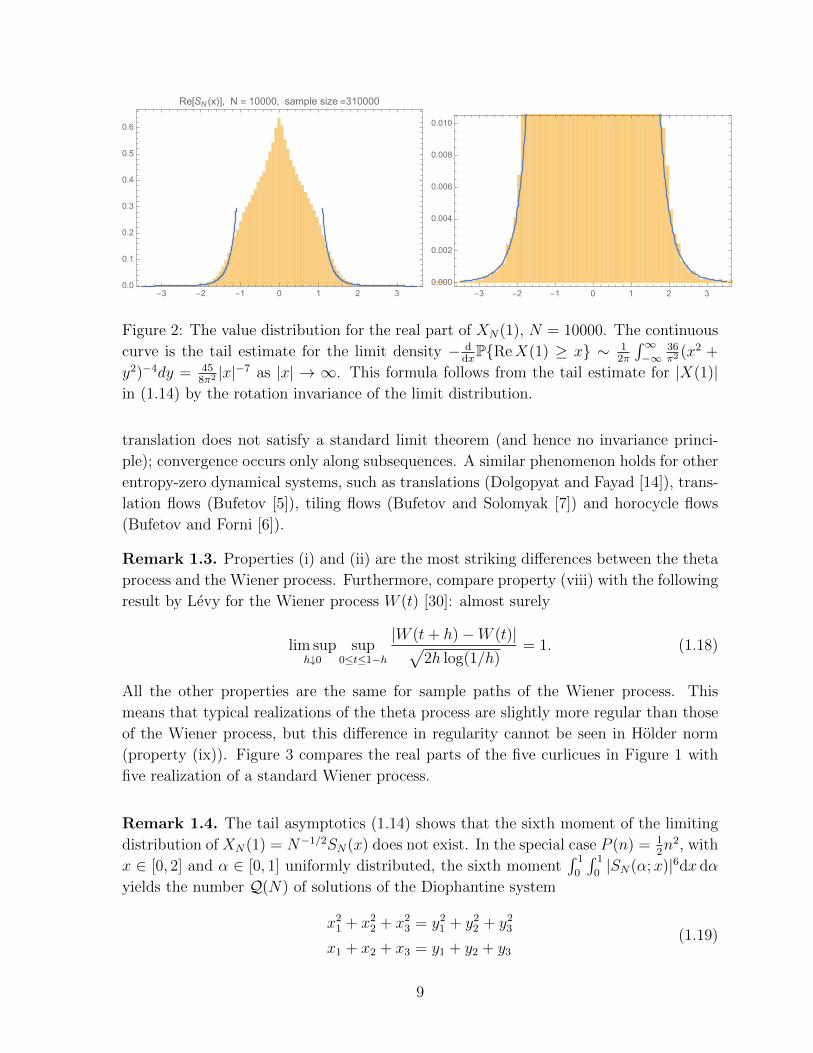
Remark 1.1. Properties (i, ii, vii) allow us to predict the distribution of |XN(t)|,Re(XN(t)), and Im(XN(t)) for large N . See Figure 2. Our approach in principle permits
a generalization of Theorems 1.3 and 1.4 to the case of rational (c1α ) ∈ Q2, however,
with some crucial differences. In particular, the tail asymptotics would now be of or-
der R−4, and stationarity and rotation-invariance of the process fail. In the special
case c1 = α = 0, a limiting theorem for the absolute value |XN(1)| = N−1/2|SN(x)|was previously obtained by Jurkat and van Horne [25], [26], [24] with tail asymptotics4 log 2π2 R−4 (see also [9, Example 75]), while the distribution for the complex random vari-
able XN(1) = N−1/2SN(x) was found by Marklof [32]; the existence of finite-dimensional
distribution of of the process t 7→ SbtNc(x) was proven by Cellarosi [10], [9]. Demirci-
Akarsu and Marklof [13], [12] have established analogous limit laws for incomplete Gauss
sums, and Kowalski and Sawin [29] limit laws and invariance principles for incomplete
Kloosterman sums and Birch sums.
Remark 1.2. If we replace the quadratic polynomial P (n) by a higher-degree polyno-
mial, no analogues of the above theorems are known. If, however, P (n) is replaced by
a lacunary sequence P (n) (e.g., P (n) = 2n), then XN(t) is well known to converge to a
Wiener process (Brownian motion). In this case we even have an almost sure invariance
principle; see Berkes [1] as well as Philipp and Stout [39]. Similar invariance princi-
ples (both weak and almost sure) are known for sequences generated by rapidly mixing
dynamical systems; see Melbourbe and Nicol [37], Gouezel [20] and references therein.
The results of the present paper may be interpreted as invariance principles for random
skew translations. Griffin and Marklof [21] have shown that a fixed, non-random skew
8
-3 -2 -1 0 1 2 30.0
0.1
0.2
0.3
0.4
0.5
0.6
Re[SN (x)], N = 10000, sample size =310000
-3 -2 -1 0 1 2 30.000
0.002
0.004
0.006
0.008
0.010
Figure 2: The value distribution for the real part of XN(1), N = 10000. The continuous
curve is the tail estimate for the limit density − ddxP{ReX(1) ≥ x} ∼ 1
2π
∫∞−∞
36π2 (x2 +
y2)−4dy = 458π2 |x|−7 as |x| → ∞. This formula follows from the tail estimate for |X(1)|
in (1.14) by the rotation invariance of the limit distribution.
translation does not satisfy a standard limit theorem (and hence no invariance princi-
ple); convergence occurs only along subsequences. A similar phenomenon holds for other
entropy-zero dynamical systems, such as translations (Dolgopyat and Fayad [14]), trans-
lation flows (Bufetov [5]), tiling flows (Bufetov and Solomyak [7]) and horocycle flows
(Bufetov and Forni [6]).
Remark 1.3. Properties (i) and (ii) are the most striking differences between the theta
process and the Wiener process. Furthermore, compare property (viii) with the following
result by Levy for the Wiener process W (t) [30]: almost surely
lim suph↓0
sup0≤t≤1−h
|W (t+ h)−W (t)|√2h log(1/h)
= 1. (1.18)
All the other properties are the same for sample paths of the Wiener process. This
means that typical realizations of the theta process are slightly more regular than those
of the Wiener process, but this difference in regularity cannot be seen in Holder norm
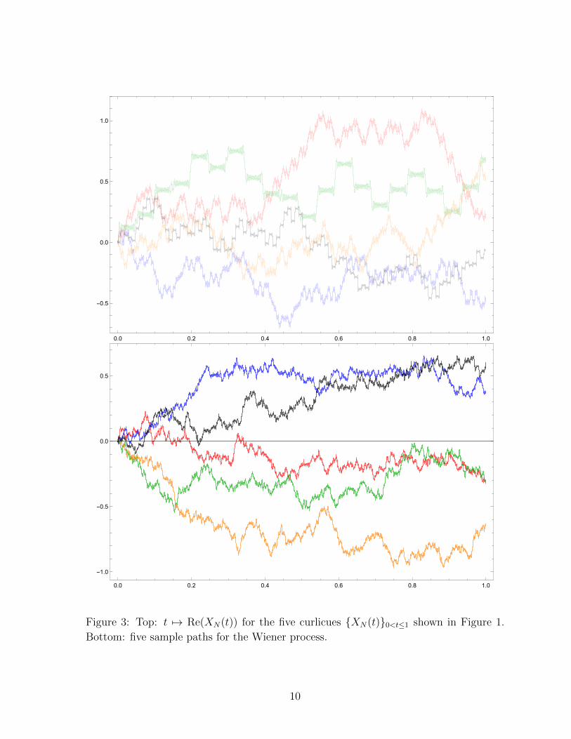
(property (ix)). Figure 3 compares the real parts of the five curlicues in Figure 1 with
five realization of a standard Wiener process.
Remark 1.4. The tail asymptotics (1.14) shows that the sixth moment of the limiting
distribution of XN(1) = N−1/2SN(x) does not exist. In the special case P (n) = 12n2, with
x ∈ [0, 2] and α ∈ [0, 1] uniformly distributed, the sixth moment∫ 1
0
∫ 1
0|SN(α;x)|6dx dα
yields the number Q(N) of solutions of the Diophantine system
x21 + x2
2 + x23 = y2
1 + y22 + y2
3
x1 + x2 + x3 = y1 + y2 + y3
(1.19)
9
0.0 0.2 0.4 0.6 0.8 1.0
-0.5
0.0
0.5
1.0
0.0 0.2 0.4 0.6 0.8 1.0
-1.0
-0.5
0.0
0.5
Figure 3: Top: t 7→ Re(XN(t)) for the five curlicues {XN(t)}0<t≤1 shown in Figure 1.
Bottom: five sample paths for the Wiener process.
10
with 1 ≤ xi, yi ≤ N (i = 1, 2, 3). Bykovskii [8] showed that Q(N) = 12π2ρ0N
3 logN +
O(N3) with
ρ0 =
∞∫−∞
∞∫−∞
∣∣∣∣1∫
0
e(uw2 − zw)dw
∣∣∣∣6dzdu. (1.20)
Using a different method, N.N. Rogovskaya [41] proved Q(N) = 18π2N
3 logN + O(N3),
which yields (without having to compute the integral (1.20) directly) ρ0 = 32. As we will
see, the integral in (1.20) also appears in the calculation of the tail asymptotics (1.14).
The currently best asymptotics for Q(N) is, to the best of our knowledge, due to V.
Blomer and J. Brudern [4].
Remark 1.5. A different dynamical approach to quadratic Weyl sums has been devel-
oped by Flaminio and Forni [18]. It employs nilflows and yields effective error estimates
in the question of uniform distribution modulo one. Their current work generalizes this
to higher-order polynomials [19], and complements Wooley’s recent breakthrough [46],
[47]. It would be interesting to see whether Flaminio and Forni’s techniques could pro-
vide an alternative to those presented here, with the prospect of establishing invariance
principles for cubic and other higher-order Weyl sums.
This paper is organized as follows. In Section 2 we define complex-valued Jacobi
theta functions, and we construct a probability space on which they are defined. The
probability space is realized as a 6-dimensional homogeneous space Γ\G. Theorem 1.1
is proven in Section 2.11 and is used in the proof of Theorem 1.2, which is carried
out in Section 3. This section also includes a new proof of Hardy and Littlewood’s
approximate functional equation (Section 3.5) and discusses several properties of the
automorphic function Θχ. In Section 4 we first prove the existence of finite-dimensional
limiting distribution for quadratic Weyl sums (Section 4.2) using equidistribution of
closed horoycles in Γ\G under the action of the geodesic flow, then we prove that the
finite dimensional distributions are tight (Section 4.3). As a consequence, the finite
dimensional distributions define a random process (a probability measure on C0), whose
explicit formula is given in Section 4.4. This formula is the key to derive all the properties
of the process listed in Theorem 1.4. Invariance properties are proved in Section 4.5,
continuity properties in Section 4.6.
Acknowledgments
We would like to thank Trevor Wooley for telling us about references [8], [41], [4],
which helped in the explicit evaluation of the leading-order constant of the tail asymp-
totics (1.14), and Emmanuel Kowalski for his comments on the manuscript. We are
furthermore grateful to the Max Planck Institute for Mathematics in Bonn for providing
11
a very congenial working environment during the program Dynamics and Numbers in
June 2014, where part of this research was carried out.
The first author gratefully acknowledges the financial support of the AMS-Simons
travel grant (2013-2014) and the NSF grant DMS-1363227. The second author thanks
the Isaac Newton Institute, Cambridge for its support and hospitality during the semester
Periodic and Ergodic Spectral Problems. The research leading to the results presented
here has received funding from the European Research Council under the European
Union’s Seventh Framework Programme (FP/2007-2013) / ERC Grant Agreement n.
291147.
2 Jacobi theta functions
This section explains how to identify the theta sums SN(x, α; f) in (1.5) with auto-
morphic functions Θf on the Jacobi group G, provided f is sufficiently regular and of
rapid decay. These automorphic functions arise naturally in the representation theory
of SL(2,R) and the Heisenberg group, which we recall in Sections 2.1–2.4. The variable
logN has a natural dynamical interpretation as the time parameter of the “geodesic”
flow on G, whereas (x, α) parametrises the expanding directions of the geodesic flow
(Section 2.5). Section 2.7 states the transformation formulas for Θf , which allows us to
represent them as functions on Γ\G, where Γ is a suitable discrete subgroup. Sections
2.8–2.10 provide more detailed analytic properties of Θf , such as growth in the cusp and
square-integrability. The proof of Theorem 1.1 is based on the exponential convergence
of nearby points in the stable direction of the geodesic flow (Section 2.11).
2.1 The Heisenberg group and its Schrodinger representation
Let ω be the standard symplectic form on R2, ω(ξ, ξ′) = xy′−yx′, where ξ = (xy) , ξ′ =(x′
y′). The Heisenberg group H(R) is defined as R2 × R with the multiplication law
(ξ, t)(ξ′, t′) =(ξ + ξ′, t+ t′ + 1
2ω(ξ, ξ′)
). (2.1)
The group H(R) defined above is isomorphic to the group of upper-triangular matrices1 x z
0 1 y
0 0 1
, x, y, z ∈ R
, (2.2)
with the usual matrix multiplication law. The isomorphism is given by
((x
y
), t
)7→
1 x t+ 12xy
0 1 y
0 0 1
. (2.3)
12
The following decomposition holds:((x
y
), t
)=
((x
0
), 0
)((0
y
), 0
)((0
0
), t− xy
2
). (2.4)
The Schrodinger representation W of H(R) on L2(R) is defined by[W
((x
0
), 0
)f
](w) = e(xw)f(w), (2.5)[
W
((0
y
), 0
)f
](w) = f(w − y), (2.6)[
W
((0
0
), t
)f
](w) = e(t)id, (2.7)
with x, y, t, w ∈ R.
For every M ∈ SL(2,R) we can define a new representation of H(R) by setting
WM(ξ, t) = W (Mξ, t). All such representations are irreducible and unitarily equivalent.
Thus for each M ∈ SL(2,R) there is a unitary operator R(M) s.t.
R(M)W (ξ, t)R(M)−1 = W (Mξ, t). (2.8)
R(M) is determined up to a unitary phase cocycle, i.e.
R(MM ′) = c(M,M ′)R(M)R(M ′), (2.9)
with c(M.M ′) ∈ C, |c(M,M ′)| = 1. If
M1 =
(a1 b1
c1 d1
), M2 =
(a2 b2
c2 d2
), M3 =
(a3 b3
c3 d3
), (2.10)
with M1M2 = M3, then
c(M1,M2) = e−iπ sgn(c1c2c3)/4. (2.11)
R is the so-called projective Shale-Weil representation of SL(2,R), and lifts to a true
representation of its universal cover SL(2,R).
2.2 Definition of SL(2,R)
Let H := {w ∈ C : Im(w) > 0} denote the upper half plane. The group SL(2,R) acts
on H by Mobius transformations z 7→ gz := az+bcz+d
, where g = ( a bc d ) ∈ SL(2,R). Every
g ∈ SL(2,R) can be written uniquely as the Iwasawa decomposition
g = nxaykφ, (2.12)
where
nx =
(1 x
0 1
), ay =
(y1/2 0
0 y−1/2
), kφ =
(cosφ − sinφ
sinφ cosφ
), (2.13)
13
and z = x+ iy ∈ H, φ ∈ [0, 2π). This allows us to parametrize SL(2,R) with H× [0, 2π);
we will use the shorthand (z, φ) := nxaykφ. Set εg(z) = (cz + d)/|cz + d|. The universal
cover of SL(2,R) is defined as
SL(2,R) := {[g, βg] : g ∈ SL(2,R), βg a continuous function on H s.t. eiβg(z) = εg(z)},(2.14)
and has the group structure given by
[g, β1g ][h, β
2h] = [gh, β3
gh], β3gh(z) = β1
g(hz) + β2h(z), (2.15)
[g, βg]−1 = [g−1, β′g−1 ], β′g−1(z) = −βg(g−1z). (2.16)
SL(2,R) is identified with H × R via [g, βg] 7→ (z, φ) = (gi, βg(i)) and it acts on H × Rvia
[g, βg](z, φ) = (gz, φ+ βg(z)). (2.17)
We can extend the Iwasawa decomposition (2.12) of SL(2,R) to a decomposition of
SL(2,R) (identified with H× R): for every g = [g, βg] ∈ SL(2,R) we have
g = [g, βg] = nxaykφ = [nx, 0][ay, 0][kφ, βkφ ]. (2.18)
For m ∈ N consider the cyclic subgroup Zm = 〈(−1, β−1)m〉, where β−1(z) = π. In
particular, we can recover the classical groups PSL(2,R) = SL(2,R)/Z1 and SL(2,R) =
SL(2,R)/Z2.
2.3 Shale-Weil representation of SL(2,R)
The Shale-Weil representation R of defined above as a projective representation of
SL(2,R) lifts to a true representation of SL(2,R) as follows. Using the decomposition
(2.18), it is enough to define the representation on each of the three factors as follows
(see [31]): for f ∈ L2(R) let
[R(nx)f ] (w) = [R(nx)f ] (w) := e(
12w2x
)f(w), (2.19)
[R(ay)f ] (w) = [R(ay)f ] (w) := y1/4f(y1/2w), (2.20)
[R(kφ)f ](w) =
f(w), if φ ≡ 0 mod 2π,
f(−w), if φ ≡ π mod 2π,
| sinφ|−1/2
∫R
e
( 12(w2 + w′2) cosφ− ww′
sinφ
)f(w′)dw′, if φ ≡/ 0 mod π,
(2.21)
14
and R(kφ) = e(−σφ/8)R(kφ). The function φ 7→ σφ is given by
σφ :=
{2ν, if φ = νπ, ν ∈ Z;
2ν + 1, if νπ < φ < (ν + 1)π, ν ∈ Z.(2.22)
and the reason for the factor e(−σφ/8) in the definition of R(kφ) is that for f ∈ S(R)
limφ→0±
[R(kφ)f ] (w) = e(±18)f(w). (2.23)
Throughout the paper, we will use the notation fφ(w) = [R(kφ)f ](w). More explicitly,
the Shale-Weil representation of SL(2,R) on L2(R) reads as
[R(z, φ)f ](w) = [R(nx)R(ay)R(kφ)f ](w) = y1/4e(12w2x)fφ(y1/2w), (2.24)
where z = x+ iy ∈ H and φ ∈ R.
2.4 The Jacobi group and its Schrodinger-Weil representation
The Jacobi group is defined as the semidirect product
SL(2,R) nH(R) (2.25)
with multiplication law
(g; ξ, ζ)(g′; ξ′, ζ ′) =(gg′; ξ + gξ′, ζ + ζ ′ + 1
2ω(ξ, gξ′)
). (2.26)
The special affine group ASL(2,R) = SL(2,R) n R2 is isomorphic to the subgroup
SL(2,R) n (R2 × {0}) of the Jacobi group and has the multiplication law
(g; ξ)(g′; ξ′) = (gg′; ξ + gξ′)) . (2.27)
For SL(2,R) 3 g = nxaykφ = (x + iy, φ) ∈ H × [0, 2π) let R(g)f := R(nx)R(ay)R(kφ)f .
If we rewrite (2.8) as
R(g)W (ξ, t) = W (gξ, t)R(g), (2.28)
then
R(g; ξ, t) = W (ξ, t)R(g) (2.29)
defines a projective representation of the Jacobi group with cocycle c as in (2.11). It
is called the Schrodinger-Weil representation. For SL(2,R) 3 [g, βg] = nxaykφ = (x +
iy, φ) ∈ H× R, we define
R(z, φ; ξ, t) = W (ξ, t)R(z, φ), (2.30)
and we get a genuine representation of the universal Jacobi group
G = SL(2,R) nH(R) = (H× R) nH(R), (2.31)
15
having the multiplication law
([g, βg]; ξ, ζ)([g′, β′g′ ]; ξ′, ζ ′) =
([gg′, β′′gg′ ]; ξ + gξ′, ζ + ζ ′ + 1
2ω(ξ, gξ′)
), (2.32)
where β′′gg′(z) = βg(g′z) + β′g′(z). The Haar measure on G is given in coordinates (x +
iy, φ; (ξ1ξ2), ζ) by
dµ(g) =dx dy dφ dξ1 dξ2 dζ
y2. (2.33)
2.5 Geodesic and horocycle flows on G
The group G naturally acts on itself by multiplication. Let us consider the action
by right-multiplication by elements of the 1-parameter group {Φt : t ∈ R} (the geodesic
flow), where
Φt =
([(e−t/2 0
0 et/2
), 0
]; 0, 0
). (2.34)
Let H+ and H− be the unstable and stable manifold for {Φs}s∈R, respectively. That is
H+ = {g ∈ G : ΦsgΦ−s → e as s→∞}, (2.35)
H− = {g ∈ G : Φ−sgΦs → e as s→∞}. (2.36)
A simple computation using (2.32) yields
H+ =
{([(1 x
0 1
), 0
];
(α
0
), 0
): x, α ∈ R
}, (2.37)
H− =
{([(1 0
u 1
), arg(u ·+1)
];
(0
β
), 0
): u, β ∈ R
}. (2.38)
We will denote the elements of H+ by n+(x, α) (see the Introduction) and those of H−by n−(u, β). We will also denote by
Ψx = n+(x, 0) =
([(1 x
0 1
), 0
]; 0, 0
)(2.39)
the horocycle flow corresponding to the unstable x-direction only.
2.6 Jacobi theta functions as functions on G
Let us consider the space of functions f : R → R for which fφ has some decay at
infinity, uniformly in φ: let us denote
κη(f) = supw,φ|fφ(w)|(1 + |w|)η. (2.40)
and define
Sη(R) :={f : R→ R
∣∣ κη(f) <∞}, (2.41)
16
see [35]. It generalizes the Schwartz space, since S(R) ⊂ Sη(R) for every η. For g ∈ Gand f ∈ Sη(R), η > 1, define the Jacobi theta function as
Θf (g) :=∑n∈Z
[R(g)f ](n). (2.42)
More explicitely, for g = (z, φ; ξ, ζ),
Θf (z, φ; ξ, ζ) = y1/4e(ζ − 12ξ1ξ2)
∑n∈Z
fφ((n− ξ2)y1/2
)e(
12(n− ξ2)2x+ nξ1
), (2.43)
where z = x + iy, ξ =(ξ1ξ2
)and fφ = R(i, φ)f . In the next section we will show that
there is a discrete subgroup Γ < G, so that Θf (γg) = Θf (g) for all γ ∈ Γ, g ∈ G. The
theta function Θf is thus well defined as a function on Γ\G.
For the original theta sum (1.10) we have
SN(x) = y−1/4Θf (x+ iy, 0; (α+c1x0 ) , c0x), (2.44)
where y = N−2 and f = 1(0,1] is the indicator function of (0, 1]. Here Θf (z, 0; ξ, ζ) is well
defined because the series in (2.43) is a finite sum. The same is true for Θf (z, φ; ξ, ζ)
when φ ≡ 0 mod π by (2.21). However, for other values of φ, the function fφ(w) decays
too slow as |w| → ∞ and we have f /∈ Sη(R) for any η > 1. For example, for φ = π/2,
fπ/2(w) = e−πi4
1∫0
e−2πiww′dw′ = eπi4
e−2πiw − 1
2πw, (2.45)
and the series (2.43) defining Θχ(z, π/2; ξ, ζ) does not converge absolutely. This illus-
trates that Θf (γ(z, 0; ξ, ζ)) may not be well-defined for general (z, 0; ξ, ζ) and γ ∈ Γ.
We shall show in Section 3 how to overcome this problem—the key step in the proof of
Theorem 1.2.
2.7 Transformation formulæ
The purpose of this section is to determine a subgroup Γ of G under which the Jacobi
theta function Θf (z, φ; ξ, ζ) is invariant. Fix f ∈ Sη, η > 1. We have the following
transformation formulæ (cf. [34]):
Θf
(−1
z, φ+ arg z;
(−ξ2
ξ1
), ζ
)= e−i
π4 Θf (z, φ, ξ, ζ) (2.46)
Θf
(z + 1, φ,
(12
0
)+
(1 1
0 1
)(ξ1
ξ2
), ζ +
ξ2
4
)= Θf (z, φ, ξ, ζ) (2.47)
Θf
(z, φ,m+ ξ, r + ζ + 1
2ω (m, ξ)
)= (−1)m1m2Θf (z, φ, ξ, ζ) , m ∈ Z2, r ∈ Z (2.48)
17
Notice that(−1
z, φ+ arg z;
(−ξ2
ξ1
), ζ
)=
([(0 −1
1 0
), arg
]; 0, 0
)(z, φ; ξ, ζ)
=(i,π
2; 0, 0
)(z, φ; ξ, ζ).
(2.49)
In other words, (2.46) describes how the Jacobi theta function Θf transforms under
left multiplication by(i, π
2; 0, 0
). Define
γ1 =
([(0 −1
1 0
), arg
]; 0,
1
8
)=
(i,π
2; 0,
1
8
), (2.50)
γ2 =
([(1 1
0 1
), 0
];
(1/2
0
), 0
)=
(1 + i, 0;
(1/2
0
), 0
), (2.51)
γ3 =
([(1 0
0 1
), 0
];
(1
0
), 0
)=
(i, 0;
(1
0
), 0
), (2.52)
γ4 =
([(1 0
0 1
), 0
];
(0
1
), 0
)=
(i, 0;
(0
1
), 0
), (2.53)
γ5 =
([(1 0
0 1
), 0
];
(0
0
), 1
)= (i, 0; 0, 1) . (2.54)
Then (2.46, 2.47, 2.48) imply that for i = 1, . . . , 5 we have Θf (γig) = Θf (g) for every
g ∈ G. The Jacobi theta function Θf is therefore invariant under the left action by the
group
Γ = 〈γ1, γ2, γ3, γ4, γ5〉 < G, . (2.55)
This means that Θf is well defined on the quotient Γ\G. Let Γ0 be the image of Γ under
the natural homomorphism ϕ : G→ G/Z ' ASL(2,R), with
Z = {(1, 2πm; 0, ζ) : m ∈ Z, ζ ∈ R}. (2.56)
Notice that Γ0 is commensurable to ASL(2,Z) = SL(2,Z) n Z2. Moreover, for fixed
(g, ξ) ∈ Γ0 we have that {([g, βg]; ξ, ζ) ∈ Γ : (g, ξ) ∈ Γ0} projects via ([g, βg]; ξ, ζ) 7→(βg(i), ζ) ∈ R × R onto {(βg(i) + kπ, k
4+ l) : k, l ∈ Z} since γ2
1 fixes the point (g, ξ).
This means that Γ is discrete and that Γ\G is a 4-torus bundle over the modular surface
SL(2,Z)\H. This implies that Γ\G is non-compact. A fundamental domain for the
action of Γ on G is
FΓ ={
(z, φ; ξ, ζ) ∈ FSL(2,Z) × [0, π)× [−12, 1
2)2 × [−1
2, 1
2)}, (2.57)
where FSL(2,Z) is a fundamental domain of the modular group in H. The hyperbolic area
of FSL(2,Z) is π3, and hence, by (2.33), we find µ(Γ\G) = µ(FΓ) = π2
3.
18
2.8 Growth in the cusp
We saw that if f ∈ Sη(R) with η > 1, then Θf is a function on Γ\G. We now observe
that it is unbounded in the cusp y > 1 and provide the precise asymptotic. Recall (2.40).
Lemma 2.1. Given ξ2 ∈ R, write ξ2 = m+ θ, with m ∈ Z and −12≤ θ < 1
2. Let η > 1.
Then there exists a constant Cη such that for f ∈ Sη(R), y ≥ 12
and all x, φ, ξ, ζ,∣∣∣∣Θf (x+ iy, φ; ξ, ζ)− y1/4e
(ζ +
(m− θ)ξ1 + θ2x
2
)fφ(−θy
12 )
∣∣∣∣ ≤ Cηκη(f) y−(2η−1)/4.
(2.58)
Proof. Since the term y1/4e(ζ + (m−θ)ξ1+θ2x
2
)fφ(−θy 1
2 ) in the left hand side of (2.58)
comes from the index n = m, it is enough to show that∣∣∣∣∣∑n 6=m
fφ
((n− ξ2)y
12
)e(
12(n− ξ2)2x+ nξ1
)∣∣∣∣∣ ≤ Cηκη(f) y−η/2. (2.59)
Indeed, ∣∣∣∣∣∑n6=m
fφ
((n− ξ2)y
12
)e(
12(n− ξ2)2x+ nξ1
)∣∣∣∣∣ ≤∑n6=m
∣∣∣fφ((n− ξ2)y12
)∣∣∣ (2.60)
≤∑n 6=m
κη(f)(1 + |n− ξ2|y
12
)η = κη(f) y−η/2∑n6=m
1
(y−1/2 + |n−m− θ|)η(2.61)
= κη(f) y−η/2∑n6=0
1
(y−1/2 + |n− θ|)η≤ Cηκη(f) y−η/2. (2.62)
Lemma 2.1 allows us derive an asymptotic for the measure of the region of Γ\G where
the theta function Θf is large. Let us define
D(f) :=
∞∫−∞
π∫0
|fφ(w)|6dφ dw. (2.63)
Lemma 2.2. Given η > 1 there exists a constant Kη ≥ 1 such that, for all f ∈ Sη(R),
R ≥ Kηκη(f),
µ({g ∈ Γ\G : |Θf (g)| > R}) =2
3D(f)R−6
(1 +Oη(κη(f)2ηR−2η)
)(2.64)
where the implied constant depends only on η.
19
Proof. Recall the fundamental domain FΓ in (2.57), and define the subset
FT ={
(x+ iy, φ; ξ, ζ) : x ∈ [−12, 1
2), y > T, φ ∈ ×[0, π), ξ ∈ [−1
2, 1
2)2, ζ ∈ [−1
2, 1
2)}.
(2.65)
We note that F1 ⊂ FΓ ⊂ F1/2. To simplify notation, set κ = Cηκη(f). We obtain an
upper bound for (2.64) via Lemma 2.1,
µ({g ∈ Γ\G : |Θf (g)| > R}) ≤ µ({g ∈ F1/2 : |Θf (g)| > R})≤ µ({g ∈ F1/2 : y1/4|fφ(−θy1/2)|+ κ y−(2η−1)/4 > R}).
(2.66)
In particular, since y1/4 + y−(2η−1)/4 ≥ y1/4|fφ(−θy1/2)| + κ y−(2η−1)/4 elements in the
above set satisfy y1/4 + y−(2η−1)/4 > R/κ, and furthermore y > 12
by the definition of
F1/2. Hence y ≥ cη(R/κ)4 for a sufficiently small cη > 0. Thus
µ({g ∈ Γ\G : |Θf (g)| > R})≤ µ({g ∈ F1/2 : y1/4|fφ(−θy1/2)|+ c−(2η−1)/4
η κ(κ/R)2η−1 > R}). (2.67)
The same argument yields the lower bound
µ({g ∈ Γ\G : |Θf (g)| > R}) ≥ µ({g ∈ F1 : |Θf (g)| > R})≥ µ({g ∈ F1 : y1/4|fφ(−θy1/2)| − c−(2η−1)/4
η κ(κ/R)2η−1 > R}). (2.68)
The terms in (2.67) and (2.68) are of the form
IT (Λ) = µ({g ∈ FT : y1/4|fφ(−θy1/2)| > Λ}), (2.69)
where T = 12
or 1 and Λ = R − c−(2η−1)/4η κ(κ/R)2η−1 or R + c
−(2η−1)/4η κ(κ/R)2η−1,
respectively. We have
IT (Λ) =
12∫
− 12
dζ
12∫
− 12
dξ1
12∫
− 12
dx
π∫0
dφ
12∫
− 12
dθ
∫y≥max(T,|fφ(−θy1/2)|−4Λ4)
dy
y2. (2.70)
By choosing the constant Kη sufficiently large, we can ensure that Λ ≥ κη(f) ≥ κ1/2(f) =
supw,φ |fφ(w)|(1+|w|)1/2. Then T ≤ |fφ(−θy1/2)|−4Λ4 and 12≥ |w||fφ(w)|2Λ−2, and using
the change of variables y 7→ w = −θy1/2, we obtain
IT (Λ) = 2
π∫0
0∫−∞
dw
|w|3
|w||fφ(w)|2Λ−2∫0
θ2dθ +
∞∫0
dw
|w|3
0∫−|w||fφ(w)|2Λ−2
θ2dθ
dφ (2.71)
=2
3Λ6
π∫0
∞∫−∞
|fφ(w)|6dw dφ, (2.72)
where Λ−6 = R−6(1 +Oη((κ/R)2η)
).
20
2.9 Square integrability of Θf for f ∈ L2(R).
Although we defined the Jacobi theta function in (2.42, 2.43) assuming that f is
regular enough so that fφ(w) decays sufficiently fast as |w| → ∞ uniformly in φ, we
recall here that Θf is a well defined element of L2(Γ\G) provided f ∈ L2(R).
Lemma 2.3. Let f1, f2, f3, f4 : R→ C be Schwartz functions. Then
1
µ(Γ\G)
∫Γ\G
Θf1(g)Θf2(g)dµ(g) =
∫R
f1(u)f2(u)du (2.73)
and
1
µ(Γ\G)
∫Γ\G
Θf1(g)Θf2(g)Θf3(g)Θf4(g)dµ(g)
=
∫R
f1(u)f2(u)du
∫R
f3(u)f4(u)du
+
∫R
f1(u)f4(u)du
∫R
f2(u)f3(u)du
.
(2.74)
Proof. The statement (2.73) is a particular case of Lemma 7.2 in [33], while (2.74) follows
from Lemma A.7 in [34].
Corollary 2.4. For every f ∈ L2(R), the function Θf is a well defined element of
L4(Γ\G). Moreover
‖Θf‖2L2(Γ\G) = µ(Γ\G)‖f‖2
L2(R), (2.75)
‖Θf‖4L4(Γ\G) = 2µ(Γ\G)‖f‖4
L2(R). (2.76)
Proof. Use Lemma 2.3, linearity in each of the fi’s and density to get the desired state-
ments for f1 = f2 = f3 = f4 = f .
2.10 Hermite expansion for fφ
In this section we use the strategy of [32] and find another representation for Θf in
terms of Hermite polynomials. We will use this equivalent representation in the proof of
Theorem 1.1 in Section 2.11.
Let Hk be the k-th Hermite polynomial
Hk(t) = (−1)ket2 dk
dtke−t
2
= k!
b k2c∑
m=0
(−1)m(2t)k−2m
m!(k − 2m)!. (2.77)
Consider the classical Hermite functions
hk(t) = (2kk!√π)−1/2e−
12t2Hk(t). (2.78)
21
For our purposes, we will use a slightly different normalization for our Hermite functions,
namely
ψk(t) = (2π)14 hk(√
2πt) = (2k−12k!)−1/2Hk(
√2π t)e−πt
2
(2.79)
The families {hk}k≥0 and {ψk}k≥0 are both orthonormal bases for L2(R, dx). Following
[32], we can write
fφ(t) =∞∑k=0
f(k)e−i(2k+1)φ/2ψk(t) (2.80)
where
f(k) = 〈f, ψk〉L2(R), (2.81)
are the Hermite coefficients of f with respect to the basis {ψk}k≥0. The uniform bound
|ψk(t)| � 1 for all k and all real t (2.82)
is classical, see [44]. It is shown in [45] that
|ψk(t)| �
{((2k + 1)1/3 + |2πt2 − (2k + 1)|
)−1/4, πt2 ≤ 2k + 1
e−γt2, πt2 > 2k + 1
(2.83)
for some γ > 0, where the implied constant does not depend on t or k. For small values
of t (relative to k) one has the more precise asymptotic
ψk(t) =23/4
π1/4((2k + 1)− 2πt2)−
14 cos
((2k+1)(2θ−sin θ)−π
4
)+O
((2k + 1)
12 (2k + 1− 2πt2)−
74
) (2.84)
where 0 ≤√
2πt ≤ (2k + 1)12 − (2k + 1)−
16 and θ = arccos
(√2πt(2k + 1)−1/2
). It will be
convenient to consider the normalized Hermite polynomials
Hk(t) = (2k−12k!)−1/2Hk(
√2πt) (2.85)
since they satisfy the antiderivative relation∫Hk(t)dt = (2π)−
12Hk+1(t)
(2k + 2)1/2. (2.86)
Lemma 2.5. Let f : R→ R be of Schwartz class. For every k ≥ 0
|f(k)| �m1
1 + kmfor every m > 1; (2.87)
22
Proof. We use integration by parts,
(2π)1/2
∫f(t)e−πt
2
Hk(t)dt =f(t)e−πt
2Hk+1(t)
(2k + 2)1/2− 1
(2k + 2)1/2
∫(Lf)(t)e−πt
2
Hk+1(t)dt,
(2.88)
where L is the operator
(Lf)(t) = f ′(t)− 2πtf(t). (2.89)
Since the function f is rapidly decreasing, the boundary terms vanish. Since Lf is also
Schwarz class, we can iterate (2.88) as many times as we want. Each time we gain a
power k−1/2. This fact yields (2.87).
The following lemma allows us to approximate fφ by f when φ is near zero. We
will use this approximation in the proof of Theorem 1.1. We will use the shorthand
Ef (φ, t) := |fφ(t)− f(t)|.
Lemma 2.6. Let f : R → R be of Schwartz class, and σ > 0. Then, for all |φ| < 1,
t ∈ R,
Ef (φ, t)�σ|φ|
1 + |t|σ. (2.90)
Proof. Assume φ ≥ 0, the case φ ≤ 0 being similar. Write
e−i(2k+1)φ/2 = 1 +O(kφ ∧ 1), (2.91)
with the notation x ∧ y := min(x, y), and by (2.80) we get
Ef (φ, t) = O
(∞∑k=0
|f(k)(kφ ∧ 1)ψk(t)|
)
= O
φ ∑0≤k≤1/φ
k|f(k)ψk(t)|
+O
∑k>1/φ
|f(k)ψk(t)|
.
(2.92)
If 1/φ < πt2−12
then by (2.83)
φ∑
0≤k≤1/φ
k|f(k)ψk(t)| � φ∑
0≤k≤1/φ
k|f(k)|e−γt2 � φ e−γt2
(2.93)
and, by (2.83, 2.84),∑k>1/φ
|f(k)ψk(t)| �∑
1/φ<k<πt2−12
|f(k)|e−γt2
+∑
k≥πt2−12
|f(k)|((2k + 1)1/3 + |2k + 1− πt2|
)−1/4
�σ φ e−γt2
+
(πt2 − 1
2
)−(σ+1)
�σ φ e−γt2
+ φ(1 + |t|σ)−1 �σ φ(1 + |t|σ)−1.
(2.94)
23
If, on the other hand, 1/φ ≥ πt2−12
, then
φ∑
0≤k≤1/φ
k|f(k)ψk(t)| � φ∑
0≤k<πt2−12
k|f(k)|e−γt2
+ φ∑
πt2−12≤k≤1/φ
k|f(k)|((2k + 1)1/3 + |2k + 1− πt2|
)−1/4
�σ φ e−γt2
+ φ(1 + |t|σ)−1 �σ φ(1 + |t|σ)−1
(2.95)
and ∑k>1/φ
|f(k)ψk(t)| �∑k>1/φ
|f(k)|e−γt2 � φ e−γt2
. (2.96)
Combining (2.92, 2.93, 2.94, 2.95, 2.96) we get the desired statement (2.90).
2.11 The proof of Theorem 1.1
Recall the notation introduced in Section 2.5. The automorphic function featured in
the statement of Theorem 1.1 is the Jacobi theta function Θf defined in (2.42).
Proof of Theorem 1.1. The fact that Θf ∈ C∞(Γ\G) for smooth f follows from (2.80)
and the estimates for the Hermite functions as shown in [32], Section 3.1. Let us then
prove the remaining part of the theorem. Recall that
SN(x, α; f) = e−s/4Θf
(x+ ie−s, 0; (α0) , 0
)= es/4Θf (n+(x, α)Φs) (2.97)
where N = es/2. Notice that
n+(x, α)n−(u, β)Φs =
(x+
u
e2s + u2+ i
es
e2s + u2, arctan(ue−s),
(α + xβ
β
),1
2αβ
).
(2.98)
We need to estimate the difference between Θf (n+(x, α)n−(u, β)Φs) and Θf (n+(x, α)Φs)
and show it depends continuously on n−(u, β) ∈ H−. To this extent, it is enough to
show continuity on compacta of H− and therefore we can assume that u and β are both
bounded. To simplify notation, we assume without loss of generality u > 0. In the
following, we will use the bounds(es
e2s + u2
)1/4
=1√N
+O
(u2
N9/2
)(2.99)(
es
e2s + u2
)1/2
=1
N+O
(u2
N5
)(2.100)
24
and
e
(1
2(n− β)2
(x+
u
e2s + u2
)+ n(α + xβ)− 1
2xβ2
)= e
(1
2n2x+ nα
)(1 +O
(un2
N4∧ 1
)),
(2.101)
where all the implied constants are uniform for N ≥ 1 and for n−(u, β) in compacta of
H−. From (2.98) we get
Θf (n+(x, α)n−(u, β)Φs) = e
(1
2αβ − 1
2(α + xβ)β
)(es
e2s + u2
) 14
×∑n∈Z
farctan(ue−s)
((n− β)
(es
e2s + u2
) 12
)e
(1
2(n− β)2
(x+
u
e2s + u2
)+ n(α + xβ)
).
(2.102)
By using (2.99) and (2.101), we obtain
Θf (n+(x, α)n−(u, β)Φs) =
(1√N
+O
(u2
N9/2
))×∑n∈Z
(∣∣∣∣∣f(
(n− β)
(es
e2s + u2
) 12
)∣∣∣∣∣+ Ef
(arctan
( u
N2
), (n− β)
(es
e2s + u2
)1/2))
× e(
1
2n2x+ nα
)(1 +O
(un2
N4∧ 1
)),
(2.103)
where Ef is as in Lemma 2.6. We claim that
∑n∈Z
f
((n− β)
(es
e2s + u2
) 12
)e
(1
2n2x+ nα
)=∑n∈Z
f( nN
)e
(1
2n2x+ nα
)+O(β) +O
(u2
N3
).
(2.104)
Indeed, by the Mean Value Theorem, the fact that f ∈ S(R), and (2.100), we have∣∣∣∣∣∑n∈Z
(f
((n− β)
(N2
N4 + u2
)1/2)− f
( nN
))e
(1
2n2x+ nα
)∣∣∣∣∣�∑n∈Z
|f ′ (τ)|(O
(β
N
)+O
(u2n
N5
))= O(β) +O
(u2
N3
) (2.105)
where τ = τ(u, β;n,N) belongs to the interval with endpoints nN
and (n−β)(
N2
N4+u2
)1/2
,
and the implied constants are uniform in N and in u, β on compacta. This proves (2.104).
25
We require two more estimates. The first uses (2.100):
∑n∈Z
∣∣∣∣∣f(
(n− β)
(es
e2s + u2
) 12
)∣∣∣∣∣O(un2
N4∧ 1
)� u
N
∑|n|≤N2/
√u
∣∣∣f( nN
)∣∣∣ ( nN
)2 1
N+
∑|n|>N2/
√u
∣∣∣f( nN
)∣∣∣= O
( uN
)+O
N ∞∫N/√u
|f(x)|dx
= O( uN
).
(2.106)
The second one uses (2.90) and (2.99, 2.100):(es
e2s + u2
)1/4∑n∈Z
Ef
(arctan
( u
N2
), (n− β)
(es
e2s + u2
)1/2)
� 1√N
u
N2
∑n∈Z
1
1 +(|n|N
)2 = O( u
N3/2
).
(2.107)
Now, combining (2.104, 2.106, 2.107), we obtain
Θf (n+(x, α)n−(u, β)Φs) = Θf (n+(x, α)Φs) +O( u
N3/2
)+O
(β
N1/2
). (2.108)
This implies (1.8) with Ef (n−(u, β)) = C(| uN|+ |β|
)for some positive constant C.
3 The automorphic function Θχ
We saw in Corollary 2.4 that Θf is a well defined element of L2(Γ\G) if f ∈ L2(R).
In this section we will consider the sharp cut-off function f = χ = 1(0,1) and find a
new series representation for Θχ by using a dyadic decomposition of the cut-off function
(Sections 3.1–3.2). We will find an explicit Γ-invariant subset D ⊂ G, defined in terms
natural Diophantine conditions (Section 3.3), where this series is absolutely convergent.
Moreover, the coset space Γ\D is of full measure in Γ\G. After proving Theorem 1.2 in
Section 3.4, we will show how it implies Hardy and Littlewood’s classical approximate
functional equation (1.2) (Section 3.5). Furthermore, we will use the explicit series
representation for Θχ to prove an analogue of Lemma 2.2 (Theorem 3.13 in section 3.6).
A uniform variation of this result is shown in Section 3.7.
26
3.1 Dyadic decomposition for Θχ
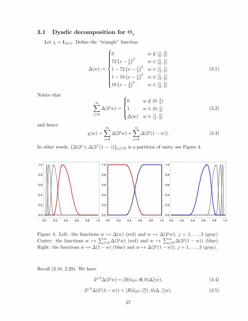
Let χ = 1(0,1). Define the “triangle” function.
∆(w) :=
0 w /∈ [16, 2
3]
72(x− 1
6
)2w ∈ [1
6, 1
4]
1− 72(x− 1
3
)2w ∈ [1
4, 1
3]
1− 18(x− 1
3
)2w ∈ [1
3, 1
2]
18(x− 2
3
)2w ∈ [1
2, 2
3]
(3.1)
Notice that
∞∑j=0
∆(2jw) =
0 w /∈ (0, 2
3)
1 w ∈ (0, 13]
∆(w) w ∈ [13, 2
3]
(3.2)
and hence
χ(w) =∞∑j=0
∆(2jw) +∞∑j=0
∆(2j(1− w)). (3.3)
In other words, {∆(2j·),∆(2j′(1− ·))}j,j′≥0 is a partition of unity, see Figure 4.
0.0 0.2 0.4 0.6 0.8 1.0
0.0
0.2
0.4
0.6
0.8
1.0
0.0 0.2 0.4 0.6 0.8 1.0
0.0
0.2
0.4
0.6
0.8
1.0
0.0 0.2 0.4 0.6 0.8 1.0
0.0
0.2
0.4
0.6
0.8
1.0
Figure 4: Left: the functions w 7→ ∆(w) (red) and w 7→ ∆(2jw), j = 1, . . . , 3 (gray).
Center: the functions w 7→∑∞
j=0 ∆(2jw) (red) and w 7→∑∞
j=0 ∆(2j(1 − w)) (blue).
Right: the functions w 7→ ∆(1− w) (blue) and w 7→ ∆(2j(1− w)), j = 1, . . . , 3 (gray).
Recall (2.18, 2.29). We have
2j/2∆(2jw) = [R(a22j ; 0, 0)∆](w), (3.4)
2j/2∆(2j(1− w)) = [R(a22j ; (01) , 0)∆−](w), (3.5)
27
where ∆−(t) := ∆(−t). Thus
χ(t) =∞∑j=0
2−j/2[R(a22j ; 0, 0)∆](t) +∞∑j=0
2−j/2[R(a22j ; (01) , 0)∆−](t). (3.6)
Let us also write the partial sums
χ(J)L =
J−1∑j=0
2−j/2[R(a22j ; 0, 0)∆](t), (3.7)
χ(J)R =
J−1∑j=0
2−j/2[R(a22j ; (01) , 0)∆−](t), (3.8)
and χ(J) = χ(J)L + χ
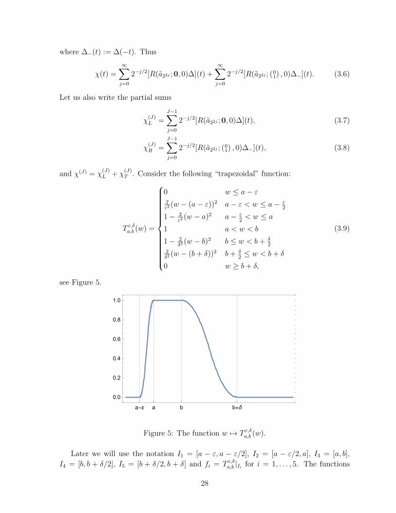
(J)T . Consider the following “trapezoidal” function:
T ε,δa,b (w) =
0 w ≤ a− ε2ε2
(w − (a− ε))2 a− ε < w ≤ a− ε2
1− 2ε2
(w − a)2 a− ε2< w ≤ a
1 a < w < b
1− 2δ2 (w − b)2 b ≤ w < b+ δ
2
2δ2 (w − (b+ δ))2 b+ δ
2≤ w < b+ δ
0 w ≥ b+ δ,
(3.9)
see Figure 5.
aa-ϵ b b+δ
0.0
0.2
0.4
0.6
0.8
1.0
Figure 5: The function w 7→ T ε,δa,b (w).
Later we will use the notation I1 = [a − ε, a − ε/2], I2 = [a − ε/2, a], I3 = [a, b],
I4 = [b, b + δ/2], I5 = [b + δ/2, b + δ] and fi = T ε,δa,b |Ii for i = 1, . . . , 5. The functions
28
χ, χ(J)L , χ
(J)R , χ(J), ∆, ∆− are all special cases of (3.9), with parameters as in the table
below.
a b ε δ
χ 0 1 0 0
χ(J)L
13·2J−1
13
16·2J−1
13
χ(J)R
23
1− 13·2J−1
13
16·2J−1
χ(J) 13·2J−1 1− 1
3·2J−11
6·2J−11
6·2J−1
∆ 13
13
16
13
∆−23
23
13
16
Lemma 3.1. There exists a constant C such that
κ2(T ε,δa,b ) = supφ,w
∣∣∣(T ε,δa,b )φ(w)∣∣∣ (1 + |w|)2 ≤ C(ε−1 + δ−1) (3.10)
for all ε, δ ∈ (0, 1] and 0 ≤ a ≤ b ≤ 1.
By adjusting C, the restriction of a, b to [0, 1] can be replaced by any other bounded
interval; we may also replace the upper bound on ε, δ by an arbitrary positive constant.
The lemma shows in particular that T ε,δa,b ∈ S2(R) for ε, δ > 0 and a ≤ b. Its proof
requires the following two estimates.
Lemma 3.2 (Second derivative test for exponential integrals, see Lemma 5.1.3 in [23]).
Let ϕ(x) be real and twice differentiable on the open interval (α, β) with ϕ′′(x) ≥ λ > 0
on (α, β). Let f(x) be real and let V = V βα (f) + maxα≤x≤β |f(x)|, where V β
α (g) denotes
the total variation of f(x) on the closed interval [α, β]. Then∣∣∣∣∣∣β∫α
e(ϕ(x))f(x)dx
∣∣∣∣∣∣ ≤ 4V√πλ. (3.11)
Lemma 3.3. Let f be real and compactly supported on [α, β], with V βα (f) < ∞. Then,
for every w, φ ∈ R,
|fφ(w)| ≤ max{3V, 2I}, (3.12)
where V = V βα (f) + maxα≤x≤β |f(x)| and I =
∫ βα|f(x)|dx.
Proof. If φ ≡ 0 mod π, then |fφ(w)| = |f(w)| ≤ V . If φ ≡ π2
mod π, then |fφ(w)| ≤ I.
If 0 < (φ mod π) < π4, let ϕ(x) =
12
(x2+w2) cosφ−wxsinφ
satisfies the hypothesis of Lemma 3.2
with λ = cotφ and we get
|fφ(w)| ≤ | sinφ|−12
4V√π cotφ
=4V√π| cosφ|
≤ 3V. (3.13)
29
The case 3π4≤ (φ mod π) < π yields the same bound by considering the complex con-
jugate of the integral before applying Lemma 3.2. If π4≤ (φ mod π) ≤ 3π
4then we have
the trivial bound
|fφ(w)| ≤ | sinφ|−12
β∫α
|f(x)|dx ≤ 2
β∫α
|f(x)|dx. (3.14)
Combining all the estimates we get (3.12).
Proof of Lemma 3.1. If φ ≡ 0 mod π, then |(T ε,δa,b )φ(w)| = |T ε,δa,b (w)| and the estimate
supw
∣∣∣(T ε,δa,b )φ(w)∣∣∣ (1 + |w|)2 = O(1) (3.15)
holds trivially.
If φ ≡ π2
mod 2π, then by (2.21), the function fφ(w) = e(−σφ/8)∫R e(−ww
′)f(w′)dw′
is (up to a phase factor) the Fourier transform of f , which reads for w 6= 0:
(T ε,δa,b )φ(w) =ie(−σφ/8)
2π3w3ε2δ2
(ε2e(−w(b+ δ))(1− e(wδ/2))2 − δ2e(−aw)(1− e(wε/2))2
),
(3.16)
and for w = 0: (T ε,δa,b )φ(0) = e(−σφ/8)2b−2a+ε+δ2
.
Similarly, if φ ≡ −π2
mod 2π, then fφ(w) = e(−σφ/8)∫R e(ww
′)f(w′)dw′, and formula
(3.16) holds with w replaced by −w.
We use the bound
|1− e(x)|2 ≤ 2|1− e(x)| ≤ 4π|x| (3.17)
applied to x = wδ/2 and x = wε/2 to conclude that, for φ ≡ π2
mod π,
|(T ε,δa,b )φ(w)| � |w|−2(δ−1 + ε−1
). (3.18)
This gives the desired bound for |w| ≥ 1. For |w| < 1, we employ instead of (3.17)
|1− e(x)|2 ≤ 4π2|x|2, (3.19)
which shows that |(T ε,δa,b )φ(w)| = O(1) in this range.
For all other φ (i.e. such that sinφ, cosφ 6= 0) we apply twice the identity
b∫a
eg(v)f(v)dv =
[eg(v) f(v)
g′(v)
]ba
−b∫
a
eg(v)
(f(v)
g′(v)
)′dv, (3.20)
30
where g(v) = 2πi12
(w2+v2) cosφ−wvsinφ
. We have
|(T ε,δa,b )φ(w)| = | sinφ|−12
∣∣∣∣∣∣∣5∑j=1
∫Ij
eg(v)fj(v)dv
∣∣∣∣∣∣∣ =| sinφ|3/2
4π2
×
∣∣∣∣∣∣∣5∑j=1
∫Ij
eg(v)3 cos2 φfj(v) + 3 cosφ(w − v cosφ)f ′j(v) + (w − v cosφ)2f ′′j (v)
(w − v cosφ)4dv
∣∣∣∣∣∣∣ . (3.21)
Let us estimate the integrals in (3.21). Consider the range |w| ≥ 3 first. The bounds
|fj(v)| ≤
{1 v ∈ [a− ε, b+ δ];
0 otherwise,(3.22)
|f ′j(v)| ≤
2ε
v ∈ [a− ε, a],2δ
v ∈ [b, b+ δ],
0 otherwise,
(3.23)
and
|f ′′j (v)| ≤
4ε2
v ∈ [a− ε, a];4δ2 v ∈ [b, b+ δ];
0 otherwise,
(3.24)
imply that5∑j=1
∫Ij
|3 cos2 φfj(v)|(w − v cosφ)4
dv �b+δ∫
a−ε
dv
(w − v cosφ)4� 1
w4, (3.25)
5∑j=1
∫Ij
∣∣3 cosφ(w − v cosφ)f ′j(v)∣∣
(w − v cosφ)4dv �
∫I1tI2
ε−1dv
|w − v cosφ|3+
∫I4tI5
δ−1dv
|w − v cosφ|3� 1
|w|3,
(3.26)5∑j=1
∫Ij
|f ′′j (v)|(w − v cosφ)2
dv �∫
I1tI2
ε−2dv
(w − v cosφ)2+
∫I4tI5
δ−2dv
(w − v cosφ)2� 1
w2(ε−1 + δ−1).
(3.27)
Therefore, for |w| ≥ 3, we have
|(T ε,δa,b )φ(w)| � 1
w2(ε−1 + δ−1) (3.28)
uniformly in all variables. For |w| < 3 we apply Lemma 3.3, which yields
|(T ε,δa,b )φ(w)| = O(1) (3.29)
since in view of (3.23) the total variation of T ε,δa,b is uniformly bounded.
31
Corollary 3.4. The series defining Θ∆(g) and Θ∆−(g) converge absolutely and uniformly
on compacta in G.
Proof. We saw that ∆ and ∆− are of the form T ε,δa,b with ε, δ > 0. The statement follows
from Lemma 3.1.
Formulæ (3.3, 3.4, 3.5) motivate the following definition of Θχ:
Θχ(g) =∞∑j=0
2−j/2Θ∆(Γg(a22j ; 0, 0)) +∞∑j=0
2−j/2Θ∆−(Γg(1; (01) , 0)(a22j ; 0, 0)). (3.30)
Each term in the above is a Jacobi theta function and, by Corollary 3.4, is Γ-invariant (cf.
Section 2.7). We will show that the series (3.30) defining Θχ(g) is absolutely convergent
for an explicit, Γ-invariant subset of G. This set projects onto a full measure set of Γ\G.
This means that we are only allow to write Θχ(Γg) only for almost every g. Therefore
Θχ is an almost everywhere defined automorphic function on the homogeneous space
Γ\G.
3.2 Hermite expansion for ∆φ
We will use here the notations from Section 2.10.
Lemma 3.5. Let ∆ : R→ R be the “triangle” function (3.1). For every k ≥ 0
|∆(k)| � 1
1 + k3/2. (3.31)
Proof. Repeat the argument in the proof of Lemma 2.5 with ∆ in place of f . In this
case we can apply (2.88) three times, and we get (3.31).
Remark 3.1. The estimate 3.31 is not optimal. One can get an additional O(k−1/4)
saving by applying (2.84) to the boundary terms after the three integration by parts.
Since the additional power saving does not improve our later results, we will simply use
(3.31).
The following lemma allows us to approximate ∆φ by ∆ when φ is near zero. We will
use this approximation in the proof of Theorem 1.2 in Section 3.4.
Lemma 3.6. Let ∆ : R→ R be the “triangle” function (3.1) and let E∆(φ, t) = |∆φ(t)−∆(t)|. For every |φ| < 1
6and every t ∈ R we have
E∆(φ, t)�
|φ|3/4, |t| ≤ 2;
|φ|3/2
1 + |t|2, |t| > 2.
(3.32)
32
Proof. Assume φ ≥ 0, the case φ ≤ 0 being similar. The estimate (3.32) for |t| > 2
follows from the proof of Lemma 3.1 (see (3.21)) and the fact that ∆ is compactly
supported. Let us then consider the case |t| < 2. We get
E∆(φ, t) = O
φ ∑0≤k≤1/φ
k|∆(k)ψk(t)|
+O
∑k>1/φ
|∆(k)ψk(t)|
. (3.33)
Since |φ| < 16, the inequality 1/φ ≥ πt2−1
2is satisfied. Therefore, by (2.83) and Lemma
3.5,
φ∑
0≤k≤1/φ
k|∆(k)ψk(t)| � φ∑
0≤k<πt2−12
k|∆(k)|e−γt2
+ φ∑
πt2−12≤k≤1/φ
k|∆(k)|((2k + 1)1/3 + |2k + 1− πt2|
)−1/4
� φe−γt2
+ φ∑
1≤k≤1/φ
k−3/4
� φ3/4
(3.34)
and ∑k>1/φ
|∆(k)ψk(t)| �∑k>1/φ
k−7/4 � φ3/4. (3.35)
Combining (3.33)-(3.35) we get the desired statement (3.32).
Remark 3.2. The statement of Lemma 3.6 is not optimal. The estimate (3.32) could
be improved for |t| < 2 to O(|φ| log(1/|φ|) by using a stronger version of Lemma 3.5, see
Remark 3.1. Since this improvement is not going to affect our results, we are content
with (3.32).
3.3 Divergent orbits and Diophantine conditions
In this section we recall a well-known fact relating the excursion of divergent geodesics
into the cusp of Γ\G and the Diophantine properties of the limit point.
A real number ω is said to be Diophantine of type (A, κ) for A > 0 and κ ≥ 1 if∣∣∣∣ω − p
q
∣∣∣∣ > A
q1+κ(3.36)
for every p, q ∈ Z, q ≥ 1. We will denote by D(A, κ) the set of such ω’s, and by D(κ)
the union of D(A, κ) for all A > 0. It is well known that for every κ > 1, the set D(κ)
has full Lebesgue measure. The elements of D(1) are called badly approximable. The set
D(1) has zero Lebesgue measure but Hausdorff measure 1.
If we consider the action of SL(2,R) on R, seen as the boundary of H, then for every
κ ≥ 1 the set D(κ) is SL(2,Z)-invariant:
33
Lemma 3.7. Let κ ≥ 1 and ω ∈ D(κ). Then for every M = ( a bc d ) ∈ SL(2,Z), Mω =aω+bcω+d
∈ D(κ).
Proof. (This is standard.) It is enough to check that the claim holds for the generators
( 1 10 1 ) and ( 0 −1
1 0 ). For the first one the statement is trivial. For the second, it suffices
to show ω ∈ D(κ) is equivalent to ω−1 ∈ D(κ). Assume without loss of generality
0 < ω < 1. Suppose first ω−1 ∈ D(A, κ) for some A > 0. Then, for 0 < p ≤ q,∣∣∣∣ω − p
q
∣∣∣∣ =ωp
q
∣∣∣∣ω−1 − q
p
∣∣∣∣ > Aω
qpκ≥ Aω
q1+κ. (3.37)
For p 6∈ (0, q], |ω− pq| ≥ min(ω, 1− ω). We have thus proved ω ∈ D(κ). To establish the
reverse implication, suppose ω ∈ D(A, κ) for some A > 0. Then, for 0 < q ≤ pdω−1e,∣∣∣∣ω−1 − q
p
∣∣∣∣ =q
ωp
∣∣∣∣ω − p
q
∣∣∣∣ > A
ωpqκ≥ A
ωdω−1eκp1+κ. (3.38)
Again we have a trivial bound for the remaining range q /∈ (0, pdω−1e]. This shows that
ω−1 ∈ D(κ).
Lemma 3.8. Let x ∈ D(A, κ) for some A ∈ (0, 1] and κ ≥ 1. Define
zs(x, u) =
(1 x
0 1
)(1 0
u 1
)(e−s/2 0
0 es/2
)i = x+
u
e2s + u2+ i
es
e2s + u2. (3.39)
Then, for s ≥ 0 and u ∈ R,
supM∈SL(2,Z)
Im(Mzs(x, u)) ≤ A−2κ e−(1− 1
κ)sW (ue−s)
≤ A−2κ e−(1− 1
κ)sW (u),
(3.40)
with
W (t) := 1 +1
2
(t2 + |t|
√4 + t2
). (3.41)
Proof. Let us set y := e−s ≤ 1. The supremum in (3.40) is achieved when Mzs(x, u)
belongs to the fundamental domain FSL(2,Z). Then
either
√3
2≤ Im(Mzs(x, 0)) < 1, or Im(Mzs(x, 0)) ≥ 1. (3.42)
In the first case we have the obvious bound Im(Mzs(x, 0)) ≤ 1. In the second case, write
M = ( a bc d ). If c = 0, then Im(Mzs(x, 0)) = y ≤ 1. If c 6= 0,
Im(Mzs(x, 0)) =y
(cx+ d)2 + c2y2≥ 1. (3.43)
This implies that (cx+ d)2/y ≤ 1 and c2y ≤ 1. The first inequality yields
y ≥ A2|c|−2κ, (3.44)
34
and therefore we have (A2
y
)1/2κ
≤ |c| ≤(
1
y
)1/2
. (3.45)
This means that
1 ≤ Im (( a bc d ) z) =y
(cx+ d)2 + c2y2≤ 1
c2y≤ A−
2κy−1+ 1
κ . (3.46)
This proves the lemma for u = 0.
Let us now consider the case of general u. Let us estimate the hyperbolic distance
between Γzs(x, 0) and Γzs(x, u) on Γ\H, which is
distΓ\H(Γzs(x, u),Γzs(x, 0)) := infM∈Γ
distH(Mzs(x, u), zs(x, 0)). (3.47)
We compute
distH(zs(x, u), zs(x, 0)) = arcosh
(1 +
(Re(z(u)− z(0))2 + (Im(z(u)− z(0))2
2 Im(z(u)) Im(z(0))
)= arcosh
(1 +
1
2u2y2
),
(3.48)
and hence
distΓ\H(Γzs(x, u),Γzs(x, 0)) ≤ arcosh
(1 +
1
2u2y2
)= log
(1 +
1
2u2y2 +
1
2|u|y
√4 + u2y2
).
(3.49)
Now,
supM∈SL(2,Z)
Im(Mzs(x, u)) ≤ supM∈SL(2,Z)
Im(Mzs(x, 0))edistΓ\H(Γzs(x,u),Γzs(x,0))
≤ supM∈SL(2,Z)
Im(Mzs(x, 0))
(1 +
1
2u2y2 +
1
2|u|y
√4 + u2y2
),
(3.50)
and the claim follows from the case u = 0.
We will in fact use the following backward variant of Lemma 3.8.
Lemma 3.9. Let x ∈ R, u ∈ R−{0} such that x+ 1u∈ D(A, κ) for some A ∈ (0, 1] and
κ ≥ 1. Then, for s ≥ 2 log(1/|u|),
supM∈SL(2,Z)
Im(Mz−s(x, u)) ≤
{max( 1
2|u| , 2) if 0 ≤ s ≤ 2 log+(1/|u|),
A−2κu1− 1
κ e−(1− 1κ
)sW (u) if s ≥ 2 log+(1/|u|),(3.51)
with log+(x) := max(log x, 0).
35
Proof. We have (1 x
0 1
)(1 0
u 1
)Φ−si =
(1 x+ 1
u
0 1
)(1 0
−u 1
)Φτ i, (3.52)
with τ = s+ log+(u2). In the range s ≥ 2 log(1/|u|), we may therefore apply Lemma 3.8
with τ in place of s, and x+ 1u
in place of x.
In the range 0 ≤ s ≤ 2 log+(1/|u|) we have Im(z−s(x, u)) = 1esu2+e−s
≥ 12. If
Im(z−s(x, u)) ≥ 1, then the maximal possible height is 12|u| . If on the other hand
12≤ Im(z−s(x, u)) < 1, then Im(Mz−s(x, u)) ≤ 2 for all M ∈ Γ.
3.4 Proof of Theorem 1.2
Let us now give a more precise formulation of Theorem 1.2 from the Introduction.
Theorem 3.10. Fix κ > 1. For x ∈ R, define
P x :=⋃A>0
P xA, P x
A :=
{n−(u, β) ∈ H− : x+
1
u∈ D(A, κ)
}. (3.53)
Then, for every (x, α) ∈ R2, h ∈ P x and s ≥ 0, the series (3.30) defining
Θχ(Γn+(x, α)hΦs) (3.54)
is absolutely convergent. Moreover, there exists a measurable function Exχ : P x → R≥0
so that
(i) for every (x, α) ∈ R2, h ∈ P x and s ≥ 0∣∣∣∣ 1√NSN(x, α)−Θχ(Γn+(x, α)hΦs)
∣∣∣∣ ≤ 1√NExχ(h), (3.55)
where N = bes/2c;
(ii) for every u0 > 1, β0 > 0, A > 0,
supx∈R
suph∈PxA∩K(u0,β0)
Exχ(h) <∞, (3.56)
with the compact subset K(u0, β0) = {n−(u, β) : u−10 ≤ |u| ≤ u0, |β| ≤ β0} ⊂ H−.
Remark 3.3. To see that Theorem 3.10 implies Theorem 1.2 notice that for every x the
set P x is of full measure in the stable horospherical subgroup H−. Let
Z = {g ∈ G : Φ−sgΦs = g for all s ∈ R}= {Φs(1; 0, t) : (s, t) ∈ R2}.
(3.57)
36
Then G = H+H−Z up to a set of Haar measure zero. By Lemma 3.7 and a short
calculation (see Lemma 3.11, Remark 3.4 below), the set
D ={n+(x, α)h ∈ G : (x, α) ∈ R2, h ∈ P x
}Z ⊂ G (3.58)
is Γ-invariant and has full measure in G.
Proof of Theorem 3.10. We assume in following that |u| ≤ u0 for an arbitrary u0 > 0.
All implied constants will depend on u0. Since χ is the characteristic function of (0, 1)
(rather than (0, 1]), we have∣∣∣SN(x, α)−√N Θχ(n+(x, α)Φs)
∣∣∣ ≤ 1 (3.59)
with s = 2 logN . Now, for every integer J ≥ 0,
J∑j=0
2−j/2(Θ∆(Γg(a22j ; 0, 0)) + Θ∆−(Γg(1; (0
1) , 0)(a22j ; 0, 0)))
= ΘT (Γg), (3.60)
where T is the trapezoidal function
T = T1
6·2J, 1
6·2J1
3·2J,1− 1
3·2J. (3.61)
Since, by Lemma 3.1, T ∈ S2(R), then the series (2.42) defining ΘT (Γg) is absolutely
convergent for every Γg ∈ Γ\G. In view of the support of T , we have
ΘT (Γn+(x, α)Φs) = Θχ(n+(x, α)Φs) (3.62)
provided 2J > 13es/2. Furthermore,
Θχ(Γn+(x, α)n−(u, β)Φs) = ΘT (n+(x, α)n−(u, β)Φs)
+∞∑
j=J+1
2−j/2Θ∆(n+(x, α)n−(u, β)Φs−(2 log 2)j)
+∞∑
j=J+1
2−j/2Θ∆−(n+(x, α)n−(u, β)Φsn−(0, 1)Φ−(2 log 2)j).
(3.63)
The proof of Theorem 3.10 therefore follows from the following estimates, which we will
derive below with the choice J = dlog2Ne:
|Θχ(n+(x, α)Φs)−ΘT (Γn+(x, α)n−(u, 0)Φs)| � |u|2/3
N1/2; (3.64)
|ΘT (n+(x, α)n−(u, β)Φs)−ΘT (n+(x, α)n−(u, 0)Φs)| = O
(|β|N1/2
); (3.65)
37
∞∑j=J+1
2−j/2∣∣Θ∆(n+(x, α)n−(u, β)Φs−(2 log 2)j)
∣∣�κFA(u)
N1/2; (3.66)
∞∑j=J+1
2−j/2∣∣Θ∆−(n+(x, α)n−(u, β)Φsn−(0, 1)Φ−(2 log 2)j)
∣∣�κFA(u)
N1/2, (3.67)
with
FA(u) = log+2 (1/|u|) max( 1
2|u| , 2)1/4 + A−1
2κu(1− 1κ
)/4W (u)1/4 max(|u|1
2κ , 1). (3.68)
Proof of (3.66) and (3.67). In view of Lemma 2.1,
∞∑j=J+1
2−j/2∣∣Θ∆(n+(x, α)n−(u, β)Φs−(2 log 2)j)
∣∣� ∞∑j=J+1
2−j/2zs−(2 log 2)j(x, u)1/4. (3.69)
and∞∑
j=J+1
2−j/2∣∣Θ∆−(n+(x, α)n−(u, β)Φsn−(0, 1)Φ−(2 log 2)j)
∣∣� ∞∑j=J+1
2−j/2zs−(2 log 2)j(x, u)1/4.
(3.70)
We divide the sum on the right and side of the above into j < J + J0 and j ≥ J + J0
with J0 = dlog+2 (1/|u|)e. The first is bounded by (apply Lemma 3.9)∑
J+1≤j<J+J0
2−j/2zs−(2 log 2)j(x, u)1/4 � 2J/2J0 max( 12|u| , 2)1/4
� N−1/2 log+2 (1/|u|) max( 1
2|u| , 2)1/4.
(3.71)
In the second range∑j≥J+J0
2−j/2zs−(2 log 2)j(x, u)1/4 � A−1
2κu(1− 1κ
)/4W (u)1/4∑
j≥J+J0
2−j/2e−(1− 1κ
)(s−(2 log 2)j)/4
�κ N−1/2A−
12κu(1− 1
κ)/4W (u)1/4 max(|u|
12κ , 1).
(3.72)
Proof of (3.64). Recall that 2J > 13es/2 and we can therefore write (3.30) as
Θχ(n+(x, α)Φs) =J∑j=0
2−j2 Θ∆(n+(x, α)Φs−(2 log 2)j)
+J∑j=0
2−j2 Θ∆−(n+(x, α)n−(0, es/2)Φs−(2 log 2)j).
(3.73)
Consider the sum in the first line of (3.73) first. We have (cf. (2.98))
n+(x, α)Φ2 logN−(2 log 2)j =
(x+ i
1
N22−2j, 0;
(α
0
), 0
). (3.74)
38
Furthermore
n+(x, α)n−(u, 0)Φ2 logN−(2 log 2)j
=
(x+
u
N42−4j + u2+ i
N22−2j
N42−4j + u2, arctan
( u
N22−2
);
(α
0
), 0
), (3.75)
so that, for 0 ≤ j ≤ J ,
Θ∆(n+(x, α)n−(u, 0)Φ2 logN−(2 log 2)j)
=
(N22−2j
N42−4j + u2
)1/4∑n∈Z
∆arctan( u
N22−2j )
(n
(N22−2j
N42−4j + u2
)1/2)
× e(
1
2n2
(x+
u
N42−4j + u2
)+ nα
).
(3.76)
Let us now proceed as in the proof of Theorem 1.1.
Θ∆(Γn+(x, α)n−(u, 0)Φ2 logN−(2 log 2)j) =
(1
(N2−j)1/2+O
(u2
(N2−j)9/2
))×∑n∈Z
[∆
(n
((N2−j)2
(N2−j)4 + u2
)1/2)
+ E∆
(arctan
(u
(N2−j)2
), n
((N2−j)2
(N2−j)4 + u2
)1/2)]
× e(
1
2n2x+ nα
)(1 +O
(|u|n2
(N2−j)4∧ 1
)). (3.77)
Using the Mean Value Theorem as in the proof of (2.104) we obtain
∑n∈Z
∆
(n
((N2−j)2
(N2−j)4 + u2
)1/2)e
(1
2n2x+ nα
)=∑n∈Z
∆( n
N2−j
)e
(1
2n2x+ nα
)+O
(u2
(N2−j)3
).
(3.78)
Analogously to (2.106) we have
∑n∈Z
∆
(n
((N2−j)2
(N2−j)4 + u2
) 12
)O
(un2
(N2−j)4∧ 1
)= O
(|u|N2−j
). (3.79)
39
Moreover, using (3.32) and the fact that∑|n|>2A
11+|n/A|2 = O(A), we have
((N2−j)2
(N2−j)4 + u2
)1/4∑n∈Z
E∆
(arctan
(u
(N2−j)2
), n
((N2−j)2
(N2−j)4 + u2
)1/2)
� 1
(N2−j)1/2
∑|n|�N2−j
(|u|
(N2−j)2
)3/4
+∑
|n|�N2−j
(|u|
(N2−j)2
)2/3
1 +∣∣ nN2−j
∣∣2
= O
(|u|3/4
N2−j
)+O
(|u|2/3
(N2−j)5/6
)= O
(|u|2/3
(N2−j)5/6
).
(3.80)
Now, combining (3.76), (3.78), (3.79), (3.80) we obtain that
Θ∆(Γn+(x, α)n−(u, 0)Φ2 logN−(2 log 2)j)
= Θ∆(Γn+(x, α)Φ2 logN−(2 log 2)j) +O
(|u|2/3
(N2−j)5/6
).
(3.81)
We can use (3.81) for 0 ≤ j ≤ J to estimate
J∑j=0
2−j/2∣∣Θ∆(n+(x, α)Φs−(2 log 2)j)−Θ∆(n+(x, α)n−(u, 0)Φs−(2 log 2)j)
∣∣� |u|
2/3
N5/6
J∑j=0
2j/3 � |u|2/3
N1/2.
(3.82)
We leave to the reader to repeat the above argument for the sum in the second line
of (3.73) and show that
J∑j=0
2−j/2∣∣Θ∆(n+(x, α)n−(0, es/2)Φs−(2 log 2)j)−Θ∆(n+(x, α)n−(u, es/2)Φs−(2 log 2)j)
∣∣� |u|
2/3
N1/2
(3.83)
Proof of (3.65). This bound follows from the Mean Value Theorem as in the proof of
(2.104).
This concludes the proof of Theorem 3.10 (and hence of Theorem 1.2).
40
3.5 Hardy and Littlewood’s approximate functional equation
To illustrate the strength of Theorem 3.10, let us show how it implies the approximate
functional equation (1.2). Recall the definition (2.50) of γ1 ∈ Γ.
Lemma 3.11. For N > 0, x > 0,
γ1n+(x, α)n−(u, β)Φ2 logN = n+(x′, α′)n−(u′, β′)Φ2 logN ′(
1; 0,1
8− α2
2x
), (3.84)
where
x′ = −1
x, N ′ = Nx, α′ =
α
x, u′ = x(1 + ux), β′ = α + βx. (3.85)
Proof. Multiplying (3.84) from the right by the inverse of n−(u, β)Φ2 logN yields
γ1n+(x, α) = n+(x′, α′)n−(u, β)Φ2 log N
(1; 0,
1
8− α2
2x
), (3.86)
where
N =N ′
N, u = u′ − uN2, β = β′ − βN. (3.87)
Multiplying the corresponding matrices in (3.86) yields
x′ = −1
x, N = u = x, α′ =
α
x, β = α. (3.88)
To conclude, we have to check that the φ-coordinates in (3.84) agree. In fact, the equality
arg
(N−2i
uN−2i+ 1+ x
)+ arg
(uN−2i+ 1
)= arg
(x(1 + ux)(xN)−2i+ 1
)(3.89)
is equivalent (since x, u,N are positive) to
arctan
(N2
u+ (N4 + u2)x
)+ arctan
( u
N2
)= arctan
(1 + ux
N2x
), (3.90)
which can be seen to hold true using the identity arctan(A)+arctan(B) = arctan(A+B1−AB
).
Remark 3.4. Note that in Lemma 3.11
x′ +1
u′= −
(x+
1
u
)−1
. (3.91)
Therefore, by Lemma 3.7, x+ 1u∈ D(κ) if and only if x′ + 1
u′∈ D(κ).
Corollary 3.12. For every 0 < x < 2 and every 0 ≤ α ≤ 1 the approximate functional
equation (1.2) holds.
41
Proof. Let us use the notation of Lemma 3.11. The invariance of Θχ under the left
multiplication by γ1 ∈ Γ, see (2.46), and Lemma 3.11 yield
Θχ
(Γn+(x, α)n−(u, β)Φ2 logN
)=√i e
(−α
2
2x
)Θχ
(Γn+(x′, α′)n−(u′, β′)Φ2 logN ′
).
(3.92)
By applying (3.55) twice with n−(u, β) ∈ P x and (by Remark 3.4) n−(u′, β′) ∈ P x′ we
obtain∣∣∣∣∣SN(x, α)−√i
xe
(−α
2
2x
)SbxNc
(−1
x,α
x
)∣∣∣∣∣≤∣∣∣SN(x, α)−
√NΘχ
(Γn+(x, α)n−(u, β)Φ2 logN
)∣∣∣+
∣∣∣∣∣√iN e
(−α
2
2x
)Θχ
(Γn+(x′, α′)n−(u′, β′)Φ2 logN ′
)−√i
xe
(−α
2
2x
)SbxNc
(−1
x,α
x
)∣∣∣∣∣≤ Ex
χ(n−(u, β)) +1√xEx′
χ (n−(u′, β′)).
(3.93)
What remains to be shown is that Exχ(n−(u, β)) and Ex′
χ (n−(u′, β′)) are uniformly bounded
in x, α over the relevant ranges. To this end, recall that u and β are free parameters
that, given x, we choose as
u =1√
5− x, β = 0. (3.94)
Then x+ 1u
=√
5 ∈ D(1) and u is bounded away from 0 and∞ for 0 < x < 2, and hence,
by (3.56), Exχ(n−(u, β)) is uniformly bounded. Furthermore, with the above choice of u,
we have
u′ =
(1
x− 1√
5
)−1
, β′ = α. (3.95)
Thus x′ + 1u′
= − 1√5∈ D(1) and u′ is bounded away from 0 and ∞ for 0 < x < 2.
Therefore, again in view of (3.56), Ex′χ (n−(u′, β′)) is uniformly bounded for 0 < x < 2,
0 ≤ α ≤ 1.
3.6 Tail asymptotic for Θχ
For the theta function Θχ we also have tail asymptotics with an explicit power saving.
Theorem 3.13. For R ≥ 1,
µ({g ∈ Γ\G : |Θχ(g)| > R}) = 2R−6(
1 +O(R−
1231
)). (3.96)
Recall the “trapezoidal” functions χ(J)L and χ
(J)R defined in (3.7, 3.8) and χ(J) =
χ(J)L + χ
(J)R . The proof of Theorem 3.13 requires the following three lemmata.
42
Lemma 3.14. Let J ≥ 1. Define
FJ(g) := Θχ
(J)L
(g) =J−1∑j=0
2−j2 Θ∆(gΦ−(2 log 2)j) (3.97)
GJ(g) := Θχ
(J)L (−·)(g) =
J−1∑j=0
2−j2 Θ∆−(gΦ−(2 log 2)j). (3.98)
Then
Θχ(g) = Θχ(J)(g) +∞∑k=1
2−kJ2
(FJ(gΦ−(2 log 2)kJ) + GJ(g(1; (0
1) , 0)Φ−(2 log 2)kJ))
(3.99)
Proof. Recall that, by Lemma 3.1, χ(J)L , χ
(J)L (−·) ∈ S2(R), and therefore the two theta
functions above are well defined for every g.
The first sum in (3.30) can be written as
∞∑j=0
2−j2 Θ∆(gΦ−(2 log 2)j) =
∞∑k=0
(k+1)J−1∑j=kJ
2−j2 Θ∆(gΦ−(2 log 2)j). (3.100)
and the k-th term in the above series is
J−1∑l=0
2−l+kJ
2 Θ∆(gΦ−(2 log 2)(l+kJ)) = 2−kJ2
J−1∑l=0
2−l2 Θ∆(gΦ−(2 log 2)kJΦ−(2 log 2)l)
= 2−kJ2FJ(gΦ−(2 log 2)kJ).
(3.101)
Similarly, the second sum in (3.30) reads as
∞∑j=0
2−j2 Θ∆−(g(1; (0
1) , 0)Φ−(2 log 2)j)
=∞∑k=0
(k+1)J−1∑j=kJ
2−j2 Θ∆−(g(1; (0
1) , 0)Φ−(2 log 2)j)
= GJ(g(1; (01) , 0)) +
∞∑k=1
2−kJ2 GJ(g(1; (0
1) , 0)Φ−(2 log 2)kJ).
(3.102)
The last thing to observe is that GJ(g(1; (01) , 0)) = Θ
χ(J)L (1−·)(g) = Θ
χ(J)R
(g). Thus
FJ(g) + GJ(g(1; (01) , 0)) = Θχ(J)(g), (3.103)
which concludes the proof of (3.99).
43
Lemma 3.15. There is a constant K such that, for all R ≥ Kδ−12J/2, 2−(J−1)/2 ≤ δ ≤ 12,
µ{g ∈ Γ\G : |Θχ(g)| > R} − µ{g ∈ Γ\G : |Θχ(J)(g)| > R(1− δ)} = O
(1
R6δ623J
),
(3.104)
µ{g ∈ Γ\G : |Θχ(J)(g)| > R(1 + δ)} − µ{g ∈ Γ\G : |Θχ(g)| > R} = O
(1
R6δ623J
).
(3.105)
Proof. We use the identity 1 = (1−δ)+2 (1−δ)2
∑∞k=1 δ
k and Lemma 3.14 for the following
union bound estimate:
µ{g ∈ Γ\G : |Θχ(g)| > R}≤ µ{g ∈ Γ\G : |Θχ(J)(g)| > R(1− δ)}
+∞∑k=1
µ{g ∈ Γ\G : |2−kJ2FJ(gΦ−(2 log 2)kJ)| > R (1−δ)
2δk} (3.106)
+∞∑k=1
µ{g ∈ Γ\G : |2−kJ2 GJ(g(1; (0
1) , 0)Φ−(2 log 2)kJ)| > R (1−δ)2δk}. (3.107)
Let us consider the sum in (3.106). We know by Lemma 3.1 that χ(J)L ∈ S2(R) with
κ2(χ(J)L ) = O(2J). We choose the constant K sufficiently large so that
R (1−δ)2δ2
J2 ≥ Kκ2(χ
(J)L ), (3.108)
holds uniformy in all parameters over the assumed ranges. This implies
R (1−δ)2δk2k
J2 ≥ Kκ2(χ
(J)L ). (3.109)
for all k. Hence, by Lemma 2.2, we can write (3.106) as
∞∑k=1
µ{g ∈ Γ\G : |Θχ
(J)L
(gΦ−(2 log 2)kJ)| > R(1− δ)
2δk2k
J2 } (3.110)
=∞∑k=1
D(χ(J)L )
R6(1− δ)6δ6k23kJO(1) = O
(1
R6δ623J
). (3.111)
The sum in (3.107) is estimated in the same way and also yields (3.111). This proves
(3.104). In order to get (3.105) we use again Lemma 3.14 and the following union bound,
44
yielding a lower bound:
µ{g ∈ Γ\G : |Θχ(g)| > R}≥ µ{g ∈ Γ\G : |Θχ(J)(g)| > R(1 + δ)}
−∞∑k=1
µ{g ∈ Γ\G : |2−kJ2FJ(gΦ−(2 log 2)kJ)| > R (1−δ)
2δk}
−∞∑k=1
µ{g ∈ Γ\G : |2−kJ2 GJ(g(1; (0
1) , 0)Φ−(2 log 2)kJ)| > R (1−δ)2δk}.
(3.112)
The last two sums are O(
1R6δ623J
)as before and we obtain (3.105).
Lemma 3.16. There is a constant K such that, for all R ≥ K2J , 0 < δ ≤ 12,
µ{g ∈ Γ\G : |Θχ(J)(g)| > R(1± δ)}
=2
3
D(χ)
R6(1 +O(δ))
(1 +O
(24JR−4
))(1 +O(2−J)). (3.113)
Proof. Lemma 2.2 implies that
µ({g ∈ Γ\G : |Θχ(J)(g)| > R(1± δ)}) =2
3
D(χ(J))
R6(1± δ)6
(1 +O
(24JR−4
))=
2
3
D(χ(J))
R6(1 +O(δ))
(1 +O
(24JR−4
)).
(3.114)
To complete the proof we need to show that
D(χ(J)) = D(χ) +O(2−J). (3.115)
The identity x6− y6 = (x2− y2)(x4 +x2y2 + y4), and the fact that χ(J)φ , χφ are uniformly
bounded (Lemma 3.3), imply
∣∣D(χ)−D(χ(J))∣∣�
∣∣∣∣∣∣π∫
0
∞∫−∞
|χφ(w)|2dw dφ−π∫
0
∞∫−∞
|χ(J)φ (w)|2dw dφ
∣∣∣∣∣∣=
∣∣∣∣∣∣π∫
0
‖χφ‖2L2dφ−
π∫0
‖χ(J)φ ‖
2L2dφ
∣∣∣∣∣∣= π
∣∣‖χ‖2L2 − ‖χ(J)‖2
L2
∣∣ ,(3.116)
by unitarity of the Shale-Weil representation. The triangle inequality yields∣∣‖χ‖2L2 − ‖χ(J)‖2
L2
∣∣ ≤ (‖χ‖L2 + ‖χ(J)‖L2
)‖χ− χ(J)‖L2 = O(2−J), (3.117)
and (3.115) follows.
45
Proof of Theorem 3.13. Combining Lemma 3.15 and Lemma 3.16 we have
µ({g ∈ Γ\G : |Θχ(g)| > R})
=2
3
D(χ)
R6(1 +O(δ))
(1 +O
(24JR−4
))(1 +O(2−J)) +O
(R−6δ−62−3J
), (3.118)
provided
R ≥ Kδ−12J/2, 2−(J−1)/2 ≤ δ ≤ 1
2. (3.119)
We set J = α log2R, δ = KR−β, with positive constants α, β,K > 0 satisfying α ≥ 2β,
α + 2β ≤ 2, K ≥√
2. Then (3.119) holds for all R ≥ 1, and
µ({g ∈ Γ\G : |Θχ(g)| > R}) =2
3
D(χ)
R6+
1
R6O(R−β +R4α−4 +R−α +R6β−3α). (3.120)
We need to work out the minimum of β, 4− 4α, α, 3α− 6β under the given constraints.
If β ≤ 3α − 6β, the largest possible value for β is 37α. Optimizing α yields α = 28
31and
thus the error term is O(R−1231 ). If on the other hand β ≥ 3α− 6β, we maximise 3α− 6β
by choosing the smallest permitted β, which is again 37α. This yields 3α− 6β = 3
7α and
we proceed as before to obtain the error O(R−1231 ).
Finally, we need to prove
D(χ) =
∞∫−∞
π∫0
|χφ(w)|6dφdw = 3. (3.121)
Recall (2.21). Using the change of variables z = w cscφ we obtain
D(χ) =
π∫0
∞∫−∞
1
| sinφ|3
∣∣∣∣∣∣1∫
0
e
(1
2w′2 cotφ− ww′ cscφ
)dw′
∣∣∣∣∣∣6
dwdφ
=
π∫0
∞∫−∞
1
| sinφ|2
∣∣∣∣∣∣1∫
0
e
(1
2w′2 cotφ− w′z
)dw′
∣∣∣∣∣∣6
dzdφ.
(3.122)
Now the change of variables u = 12
cotφ yields
D(χ) = 2
∞∫−∞
∞∫−∞
∣∣∣∣∣∣1∫
0
e(uw′2 − zw′)dw′∣∣∣∣∣∣6
dzdu = 3, (3.123)
cf. [41]. This concludes the proof of (3.96).
46
3.7 Uniform tail bound for Θχ
The goal of this section is to obtain a result, similar to Theorem 3.13, for the tail
distribution of |Θχ(x+ iy, 0; ξ, ζ)| uniform in all variables. Namely the following
Proposition 3.17. Let λ be a Borel probability measure on R which is absolutely con-
tinuous with respect to Lebesgue measure. Then
λ({x ∈ R : |Θχ(x+ iy, 0; ξ, ζ)| > R})� 1
(1 +R)4, (3.124)
uniformly in y ≤ 1, R > 0, and (ξ, ζ) ∈ H(R).
This proposition will be used in Section 4.3 to show that the finite dimensional
limiting distributions for XN(t) are tight. The proof of Proposition 3.17 requires three
lemmata. First, let us define Γ = PSL(2,Z) and Γ∞ = {( 1 m0 1 ) : m ∈ Z}. For z ∈ H and
γ ∈ Γ∞\Γ set yγ = Im(γz) and define
H(z) =∑
γ∈Γ∞\Γ
y1/4γ χ[ 1
2,∞)(y
1/4γ ). (3.125)
We note that this sum has a bounded number of terms, and H(γz) = H(z). H may thus
be viewed as a function on Γ\H. Since Γ\G is a fibre bundle over the modular surface
Γ\H (recall Section 2.7), we may furthermore identify H with a Γ-invariant function on
G by setting H(g) := H(z) with g = (x+ iy, φ; ξ, ζ).
Lemma 3.18. Let f ∈ Sη(R), η > 1. Then, for every g ∈ G, we have
|Θf (g)| ≤ C1H(g), (3.126)
where C1 = κ0(f) + C ′1κη(f) and C ′1 > 0 is some absolute constant.
Proof. Lemma 2.1 implies that |Θf (x+ iy, φ; ξ, ζ)| ≤ C1y14 uniformly in all variables for
y ≥ 12, and thus uniformly for all points in the fundamental domain FΓ. By definition,
H(x + iy) is a sum of positive terms and y1/4 is one of them if y ≥ 12. Hence y
14 ≤
H(x+ iy).
The following lemma estimates how much of the closed horocycle {x+ iy : −12≤ x ≤
12} is above a certain height in the cusp.
Lemma 3.19. Let R ≥ 1 and r(y) = 1{y1/4>R}. Then, for every y ≤ 1,
1∫0
∑γ∈Γ∞\Γ
r(yγ)dx ≤ 2R−4 (3.127)
47
Proof. For z = x + iy we have Im(( a bc d ) z) = y|cz+d|2 . Thus, writing d = d′ + mc with
1 ≤ d′ ≤ d− 1, we get∑γ∈Γ∞\Γ
r(yγ) = r(y) +∑
(c, d) = 1
c > 0
d ∈ Z
r
(y
|cz + d|2
)
= r(y) +∞∑c=1
∑d′ mod c
(c, d′) = 1
∑m∈Z
r
(y
c2∣∣z + d′
c+m
∣∣2).
(3.128)
So
1∫0
∑γ∈Γ∞\Γ
r(yγ)dx = r(y) +∞∑c=1
∑d′ mod c
(c, d′) = 1
∞∫−∞
r
(y
c2|x+ iy|2
)dx. (3.129)
A change of variables allows us to write the last integral as
∞∫−∞
r
(y
c2|x+ iy|2
)dx = y
∞∫−∞
r
(1
c2y(x2 + 1)
)dx = yr(c2y), (3.130)
where
r(t) =
∞∫−∞
r
(1
t(x2 + 1)
)dx =
∫{x∈R: t(x2+1)<R−4}
dx =
2√
1R4t− 1 if R−4 > t,
0 otherwise.(3.131)
Now (3.129) equals
r(y) + 2y∑c ≥ 1
c2y < R−4
∑d′ mod c
(c, d′) = 1
√1
R4c2y− 1. (3.132)
Since y ≤ 1 we have r(y) = 0 and (3.132) is
≤ 2y12R−2
∑c ≥ 1
c2y < R−4
∑d′ mod c
(c, d′) = 1
1
c(3.133)
≤ 2y12R−2
∑c ≥ 1
c2y < R−4
1 = 2y12R−2
⌊√1
yr4
⌋≤ y
12R−2
√1
yR4= 2R−4. (3.134)
48
Lemma 3.20. Let f ∈ Sη(R), η > 1, and λ as in Proposition 3.17.
λ({x ∈ R : |Θf (x+ iy, φ; ξ, ζ)| > R})� (1 +R)−4, (3.135)
uniformly in y ≤ 1, R > 0, and all φ, ξ, ζ.
Proof. Lemma 3.18 yields∫R
1{|Θf (x+iy,φ;ξ,ζ)|>R}λ(dx) ≤∫R
1{H(x+iy)> RC1}λ(dx). (3.136)
Since H(z + 1) = H(z), we have∫R
1{H(x+iy)> RC1}λ(dx) =
∫R/Z
1{H(x+iy)> RC1}λZ(dx) (3.137)
where λZ is the push forward under the map R→ R/Z, x 7→ z+Z. Since λ is absolutely
continuous, so is λZ (with respect to Lebesgue measure on R/Z) and we have∫R/Z
1{H(x+iy)> RC1}λZ(dx)�
∫R/Z
1{H(x+iy)> RC1}dx. (3.138)
Now, for R ≥ C1 we have∫R/Z
1{H(x+iy)> RC1}dx =
∑γ∈Γ∞\Γ
1{y
1/4γ > R
C1
}dx ≤ 2C41R−4 (3.139)
in view of Lemma 3.19. As the left hand side of (3.135) is bounded trivially by 1 for all
R < C1, the proof is complete.
Proof of Proposition 3.17. Write
Θχ(x+ iy, 0; ξ, ζ) =J∑j=0
2−j2 Θ∆((x+ iy, 0; ξ, ζ)Φ−(2 log 2)j) (3.140)
+J∑j=0
2−j2 Θ∆−((x+ iy, 0; ξ, ζ)(1; (0
1) , 0)Φ−(2 log 2)j) (3.141)
where J = dlog2 y−1/2e. Set
δj :=3
2π2
1
j2(1 ≤ j ≤ J), δ0 :=
1
2−
J∑j=1
δj. (3.142)
49
Notice that 14< δ0 ≤ 1
2− 3
2π2 and 2∑J
j=0 δj = 1. In order to handle the two sums (3.140)
and (3.141) we use a union bound as in the proof of Lemma 3.15 and apply Lemma 3.20.
We obtain
λ({x ∈ R : |Θχ(x+ iy, 0; ξ, ζ)| > R})
≤dlog y−1e∑j=0
λ({x ∈ R : |Θ∆((x+ iy, 0; ξ, ζ)Φ−(2 log 2)j)| > 2j2 δjR})
+
dlog y−1e∑j=0
λ({x ∈ R : |Θ∆−((x+ iy, 0; ξ, ζ)(1; (01) , 0)Φ−(2 log 2)j)| > 2
j2 δjR})
�dlog y−1e∑j=0
1
(1 + 2j2 δjR)4
≤ R−4
dlog y−1e∑j=0
2−2jδ−4j � R−4
(3.143)
uniformly in y. This bound is useful for R ≥ 1. For R < 1 we use the trivial bound
λ({. . .}) ≤ 1.
4 Limit theorems
We now apply the findings of the previous two main sections to prove the invariance
principle for theta sums, Theorem 1.3. Following the strategy of [32], we first estab-
lish that the random process XN(t) converges in finite-dimensional distribution to X(t)
(Section 4.2). The proof exploits equidistribution of translated horocycle segments on
Γ\G, which we derive in Section 4.1 using theorems of Ratner [40] and Shah [42]. Tight-
ness of the sequence of processes XN(t) is obtained in Section 4.3; it follows from the
uniform tail bound for Θχ (Section 3.7). Convergence in finite-dimensional distribution
and tightness yield the invariance principle for XN(t). The limiting process X(t) has
a convenient geometric interpretation in terms of a random geodesic in Γ\G (Section
4.4), from which the invariance and continuity properties stated in Theorem 1.4 can be
extracted; cf. Sections 4.5–4.6.
4.1 Equidistribution theorems
Recall that G = SL(2,R) n H(R), and define ASL(2,Z) = SL(2,R) n R2 as in [34].
Throughout this section, we assume that Γ is a lattice in G such that Γ0 = ϕ(Γ) is
commensurable with ASL(2,Z). An example of such Γ is the one defined in (2.55). We
have the following equidistribution theorems. Let Φt and Ψu be as in section 2.5.
Theorem 4.1. Let F : Γ\G → R be bounded continuous and λ a Borel probability
measure on R which is absolutely continuous with respect to Lebesgue measure. For any
50
M ∈ SL(2,R), ξ ∈ R2 \Q2 and ζ ∈ R we have
limt→∞
∫R
F (Γ(M ; ξ, ζ)ΨuΦt)dλ(u) =1
µ(Γ\G)
∫Γ\G
F (g)dµ(g). (4.1)
Proof. By a standard approximation argument it is sufficient to show that, for every
−∞ < a < b <∞, the curve
Ct = {Γ(M ; ξ, ζ)ΨuΦt) : u ∈ [a, b]} (4.2)
becomes equidistributed in Γ\G with respect to µ. In other words, the uniform proba-
bility measure νt on the orbit Ct converges weakly to µ (appropriately normalised). We
know from [15] (cf. also [36]) that for ξ ∈ R2 \Q2 the projection ϕ(Ct) becomes equidis-
tributed in Γ0\ASL(2,R), where Γ0 = ϕ(Γ) is commensurable with ASL(2,Z). Since
Γ\G is a compact extension of Γ0\ASL(2,R), this imples that (a) the sequence (νt)t is
tight and (b) the support of any possible weak limit ν projects to Γ0\ASL(2,R). Again
a classic argument (cf. [15, 42]) shows that ν is invariant under the right action of Ψu.
Therefore, by Ratner’s measure classification argument [40], every ergodic component
of ν is supported on the orbit Γ\ΓH for some closed connected subgroup H ≤ G. By
(b) we know that Γ\ΓH must project to Γ0\ASL(2,R) and hence ϕ(H) = G/Z. The
only subgroup H ≤ G which satisfies ϕ(H) = G/Z is, however, H = G and hence every
ergodic component of ν equals µ for any possible weak limit, i.e., ν = µ (up to normal-
isation). Therefore the limit is unique, which in turn implies that every subsequence in
(νt)t converges.
Theorem 4.2. Let F : R × Γ\G → R be bounded continuous and λ a Borel probability
measure on R which is absolutely continuous with respect to Lebesgue measure. Let
Ft : R × Γ\G → R be a family of uniformly bounded, continuous functions so that
Ft → F , uniformly on compacta. For any M ∈ SL(2,R), ξ ∈ R2 \Q2 and ζ ∈ R we have
limt→∞
∫R
Ft(u,Γ(M ; ξ, ζ)ΨuΦt)dλ(u) =1
µ(Γ\G)
∫R×Γ\G
F (u, g)dλ(u)dµ(g). (4.3)
Proof. This follows from Theorem 4.1 by a standard argument, see [36, Theorem 5.3].
Corollary 4.3. Let F , Ft and λ be as in Theorem 4.2. For any (α, β) ∈ R2 \ Q2 and
ζ, γ ∈ R we have
limt→∞
∫R
Ft(u,Γ
(1;(α+uβ
0
), ζ + uγ
)ΨuΦt
)dλ(u) =
1
µ(Γ\G)
∫R×Γ\G
F (u, g)dλ(u)dµ(g).
(4.4)
Proof. We have(1;(α+uβ
0
), ζ + uγ
)ΨuΦt = (1; ( α
−β) , ζ) Ψu(1;(
0β
), uγ − β(α + uβ)
)Φt
= (1; ( α−β) , ζ) ΨuΦt
(1;(
0e−t/2β
), uγ − β(α + uβ)
).
(4.5)
51
Define
Ft(u, g) = Ft(u, g
(1;(
0e−t/2β
), uγ − β(α + uβ)
)), (4.6)
F (u, g) = F (u, g (1; 0, uγ − β(α + uβ))) . (4.7)
Since right multiplication is continuous and commutes with left multiplication, we see
that, under the assumptions on Ft, Ft is a family of uniformly bounded, continuous
functions R×Γ\G→ R so that Ft → F , uniformly on compacta. Theorem 4.2 therefore
yields
limt→∞
∫R
Ft(u,Γ
(1;(α+uβ
0
), ζ + uγ
)ΨuΦt
)dλ(u) =
1
µ(Γ\G)
∫R×Γ\G
F (u, g)dλ(u)dµ(g).
(4.8)
Finally, the invariance of µ under right multiplication by (1; 0, ζ), for any ζ ∈ R, shows
that ∫R×Γ\G
F (u, g)dλ(u)dµ(g) =1
µ(Γ\G)
∫R×Γ\G
F (u, g)dλ(u)dµ(g). (4.9)
4.2 Convergence of finite-dimensional distributions
In this section we prove the convergence of the finite dimensional distributions for the
random curves (1.11). This means that, for every k ≥ 1, every 0 ≤ t1 < t2 < · · · < tk ≤ 1,
and every bounded continuous function B : Ck → R,
limN→∞
∫R
B(XN(x; t1), . . . , XN(x; tk))h(x)dx
=1
µ(Γ\G)
∫Γ\G
B(√t1Θχ(gΦ2 log t1), . . . ,
√tkΘχ(gΦ2 log tk)) dµ(g) (4.10)
Recall that, by (1.11, 2.44),
XN(x; t) = es/4Θf (x+ iye−s, 0; (α+c1x0 ) , c0x) +
{tN}√N
(SbtNc+1(x)− SbtNc(x)
), (4.11)
where s = 2 log t, y = N−2 and f = 1(0,1]. It will be more convenient to work with
XN(x; t) = es/4Θχ(x+ iye−s, 0; (α+c1x0 ) , c0x), (4.12)
where χ = 1(0,1). We have |XN(t) − XN(t)| ≤ 3N−1/2 for all t and N . Therefore, it is
enough to show that the limit (4.10) holds for XN(x; t) in place of XN(x; t). We can
write
XN(x; t) = es/4Θχ((1; (α+c1x0 ) , c0x) ΨxΦτΦs) , (4.13)
52
where τ = − log y.
To simplify notation, we will write in the following Θf,s(g) := es/4Θf (gΦs), g ∈ G.
Observe that Θf,s is also well defined on Γ\G. Moreover, for every k ∈ N and every
s = (s1, s2, . . . , sk) ∈ Rk with s1 < s2 < · · · < sk, let us define
Θf,s : Γ\G→ Ck, Θf,s(g) := (Θf,s1(g),Θf,s2(g), . . . ,Θf,sk(g)) . (4.14)
With this we have, for 0 < t1 < t2 < . . . < tk ≤ 1,(XN(x; t1), . . . , XN(x; tk)
)= Θχ,s((1; (α+c1x
0 ) , c0x) ΨxΦτ ) (4.15)
with sj = 2 log tj and τ = 2 logN . The weak convergence of finite dimensional distribu-
tion of the process XN(t) stated in (4.10) is a consequence of the above discussion and
the following
Theorem 4.4. Let λ be a Borel probability measure on R which is absolutely continuous
with respect to Lebesgue measure. Let c1, c0, α ∈ R with (α, c1) /∈ Q2. Then for every
k ≥ 1, every s = (s1, s2, . . . , sk) ∈ Rk, and every bounded continuous function B : Ck →R
limτ→∞
∫R
B(Θχ,s((1; (α+c1x0 ) , c0x)ΨxΦτ )) dλ(x) =
1
µ(Γ\G)
∫Γ\G
B(Θχ,s(g))dµ(g). (4.16)
We first prove a variant of this statement for smooth cut-off sums, with Θχ,s replaced
Θf,s, where f ∈ Sη, η > 1.
Lemma 4.5. Let f ∈ Sη(R), with η > 1. Under the assumptions of Theorem 4.4, for
every k ≥ 1, every s = (s1, s2, . . . , sk) ∈ Rk, and every bounded continuous function
B : Ck → R
limτ→∞
∫R
B(Θf,s((1; (α+c1x0 ) , c0x)ΨxΦτ )) dλ(x) =
1
µ(Γ\G)
∫Γ\G
B(Θf,s(g))dµ(g). (4.17)
Proof. Apply Corollary 4.3 with Ft(u, g) = F (u, g) = B(Θf,s(g)) (no dependence on
t, u), β = c1, γ = c0, and ζ = 0.
Lemma 4.5 implies Theorem 4.4 via a standard approximation argument that requires
the following lemmata. We first consider the variance. For z = (z1, . . . , zk) ∈ Ck, let
‖z‖Ck = (|z1|2 + . . .+ |zk|2)1/2.
Lemma 4.6. Let f , h be compactly supported, Riemann-integrable functions on R, and
assume h ≥ 0. Then, for all α, c1, c0 ∈ R,
lim supτ→∞
∫R
‖Θf,s((1; (α+c1x0 ) , c0x)ΨxΦτ )‖2
Ck h(x)dx ≤ 2k‖f‖2L2‖h‖L1 . (4.18)
53
Proof. By a standard approximation argument, we may assume without loss of generality
that h ∈ C2c (R). The Fourier transform h of h then satisfies the bound |h(y)| � |y|−2.
We have, by Parseval’s identity,∫R
‖Θf,s((1; (α+c1x0 ) , c0x)ΨxΦτ )‖2
Ck h(x)dx
= y12
k∑j=1
esj/2∑n,m∈Z
f(ny12 e−sj/2) f(my
12 e−sj/2) e((n−m)α) h
(12(m2 − n2) + c1(m− n)
)≤ y
12
k∑j=1
esj/2∑n,m∈Z
∣∣∣f(ny12 e−sj/2) f(my
12 e−sj/2) h
(12(m2 − n2) + c1(m− n)
)∣∣∣ ,(4.19)
where y = e−τ . Note that (m2 − n2) + 2c1(m − n) = (m − n)(m + n + 2c1) = 0 if and
only if [m = n or m = −n − 2c1]. The sum restricted to m = n is a Riemann sum. In
the limit y → 0,
y12
k∑j=1
esj/2∑n∈Z
∣∣∣f(ny12 e−sj/2) f(ny
12 e−sj/2)
∣∣∣→ k‖f‖2L2‖h‖L1 . (4.20)
Likewise, the sum restricted to m = −n− 2c1 yields
y12
k∑j=1
esj/2∑n∈Z
∣∣∣f(ny12 e−sj/2) f(−(n+ 2c1)y
12 e−sj/2)
∣∣∣→ k
∫R
|f(w)f(−w)|dw ‖h‖L1
≤ k‖f‖2L2‖h‖L1 .
(4.21)
The sum of the remaining terms with (m2 − n2) + 2c1(m− n) 6= 0 is bounded above by
(set p = m− n, q = m+ n and overcount by allowing all p, q ∈ Z with p 6= 0, q 6= −2c1)
y12
k∑j=1
esj/2∑p,q∈Zp 6=0
q 6=−2c1
∣∣∣f(12(q − p)y
12 e−sj/2) f(1
2(q + p)y
12 e−sj/2) h
(12p(q + 2c1)
)∣∣∣
� y12
k∑j=1
esj/2∑p,q∈Zp 6=0
q 6=−2c1
|p(q + 2c1)|−2 = O(y12 ).
(4.22)
Hence all “off-diagonal” contributions vanish as y → 0.
For the rest of this section assume that λ is a Borel probability measure on R which
is absolutely continuous with respect to Lebesgue measure.
54
Lemma 4.7. Let f be a compactly supported, Riemann-integrable function on R. Then,
for all α, c1, c0 ∈ R, K > 0,
lim supτ→∞
λ({x ∈ R : ‖Θf,s((1; (α+c1x
0 ) , c0x)ΨxΦτ )‖Ck > K})
<4k2‖f‖2
L2
K2. (4.23)
Proof. Let us denote by λ′ ∈ L1(R) the probability density of λ, and by mh the measure
with density h ∈ Cc(R), h ≥ 0. We have
λ({x ∈ R : ‖Θf,s((1; (α+c1x
0 ) , c0x)ΨxΦτ )‖Ck > K})
≤ mh
({x ∈ R : ‖Θf,s((1; (α+c1x
0 ) , c0x)ΨxΦτ )‖Ck > K})
+ ‖λ′ − h‖L1
< 4k2K−2‖f‖2L2‖h‖L1 + ‖λ′ − h‖L1
(4.24)
by Chebyshev’s inequality and Lemma 4.6. Since Cc(R) is dense in L1(R), rel. (4.23)
follows.
Lemma 4.8. For all α, c1, c0 ∈ R and ε > 0 there exists a constant Kε > 0 such that
lim supτ→∞
λ({x ∈ R : ‖Θf,s((1; (α+c1x
0 ) , c0x)ΨxΦτ )‖Ck > Kε
})≤ ε‖f‖2
L2 (4.25)
for every compactly supported, Riemann-integrable f .
Proof. It follows immediately from Lemma 4.7.
Lemma 4.9. Let f be a compactly supported, Riemann-integrable function on R. Then,
for every ε > 0, δ > 0 there exists f ∈ S2(R) with compact support such that
lim supτ→∞
λ({x ∈ R : ‖Θf,s((1; (α+c1x
0 ) , c0x)ΨxΦτ )−Θf ,s((1; (α+c1x0 ) , c0x)ΨxΦτ ) ‖Ck > δ
})< ε. (4.26)
Proof. Note that Θf,s−Θf ,s = Θf−f ,s. Since f− f is compactly supported and Riemann-
integrable, we can apply Lemma 4.7 with f − f in place of f . Choose K = ε and f so
that4k2‖f − f‖2
L2
K2≤ δ, (4.27)
which is possible since S2(R) is dense in L2(R). The claim follows.
Proof of Theorem 4.4. Lemma 4.8 and Helly-Prokhorov’s Theorem imply that every se-
quence (τj)j≥1 such that τj →∞ as j →∞ has a subsequence (τjl)l≥1 with the following
property: there is a probability measure ν on C such that for every bounded continuous
function B : Ck → C we have
liml→∞
∫R
B(Θχ,s((1; (α+c1x0 ) , c0x)ΨxΦτjl )) dλ(x) =
∫C
B(z)dν(z). (4.28)
55
The measure ν may of course depend on the choice of the subsequence. To identify that
measure, we restrict to test functions B ∈ C∞c (Ck). We claim that for such B the limit
I(χ) = limj→∞
∫R
B(Θχ,s((1; (α+c1x0 ) , c0x)ΨxΦτj)) dλ(x) (4.29)
exists. To prove this, let us first notice that, since B ∈ C∞c (Ck), it is Lipschitz, i.e.
|B(z′)−B(z′′)| ≤ C‖z′− z′′‖Ck for some constant C > 0. Therefore, by Lemma 4.9, for
every ε > 0, δ > 0, we can find a compactly supported f ∈ Sη(R) with η > 1 such that∫R
|B(Θχ,s((1; (α+c1x0 ) , c0x)ΨxΦτj))−B(Θf,s((1; (α+c1x
0 ) , c0x)ΨxΦτj)) |dλ(x)
≤ C
∫R
‖Θχ,s((1; (α+c1x0 ) , c0x)ΨxΦτj)−Θf,s((1; (α+c1x
0 ) , c0x)ΨxΦτj) ‖Ckdλ(x)
≤ C(ε+ δ).
(4.30)
Since the limit
I(f) = limj→∞
∫R
B(Θf,s((1; (α+c1x0 ) , c0x)ΨxΦτj)) dλ(x) (4.31)
exists by Lemma 4.5, the sequence∫R
B(Θf,s((1; (α+c1x0 ) , c0x)ΨxΦτj)) dλ(x)
j≥1
(4.32)
is Cauchy. Using this fact, the bound (4.30) and the triangle inequality, we see that∫R
B(Θχ,s((1; (α+c1x0 ) , c0x)ΨxΦτj)) dλ(x)
j≥1
(4.33)
is a Cauchy sequence, too, and hence the limit I(χ) exists as claimed. The bound (4.30)
implies that I(f) → I(χ) as f → χ in L2 and therefore the right-hand side of (4.28)
must equal the right-hand side of (4.16).
We have now established that, for any convergent subsequence, the weak limit ν in
(4.28) in fact unique, i.e. the same for every converging subsequence. This means that
every subsequence converges—in particular the full sequence. This concludes the proof
of the theorem.
4.3 Tightness
The purpose of this section is to prove that the family of processes {XN}N≥1 is tight.
Recall that each XN is a random variable with values on the Polish space (C0, d), cf.
56
(1.11). If we denote by PN the probability measure induced by XN on C0, then tightness
means that for every ε > 0 there exists a compact set Kε ⊂ C0 with PN(Kε) > 1− ε for
every N ≥ 1. We prove the following
Proposition 4.10. The sequence {XN}N≥1 is tight.
Proof. For every K > 0 and every positive integer N set
MK,N =
{x ∈ R : ∃m ≥ 1 and 0 ≤ k < 2m s.t.
∣∣∣∣XN
(k + 1
2m
)−XN
(k
2m
)∣∣∣∣ > K
m2
},
(4.34)
We will prove the tightness of the process t 7→ XN(t) by establishing that
limK→∞
supN≥1
λ(MK,N) = 0. (4.35)
To see that (4.35) is equivalent to tightness, recall how the curve t 7→ XN(t) depends on
x (cf. (1.10), (1.11)) and observe that functions in the set
C0 r⋃K>0
{XN : [0, 1]→ C | x ∈MK,N} (4.36)
are uniformly equicontinuous on a dense set (of dyadic rationals). Since in our case
XN(0) = 0 by definition, uniform equicontinuity is equivalent to tightness (see [3], The-
orem 7.3).
Let us now show (4.35). By construction,∣∣∣∣XN
(k + 1
2m
)−XN
(k
2m
)∣∣∣∣ ≤√N
2m. (4.37)
Therefore, if m > 0 is such that√N
2m≤ 1
m2 for all N ≥ 1, then the inequality defining
(4.34) has no solution for all K > 1. For N = 1 the inequality is m2
2m≤ 1 is valid for
every m ≥ 4. For N ≥ 2 a sufficient condition for m2
2m≤ 1√
Nis m > 5 log2N . Thus, it is
enough to restrict the range of m in (4.34) to 1 ≤ m ≤ 5 log2N . For these values of m,
let us estimate the measure of MK,N from above by estimating the measure of{x ∈ R :
∣∣∣∣XN
(k + 1
2m
)−XN
(k
2m
)∣∣∣∣ > K
m2
}(4.38)
for fixed m and k. Define N1 = k2mN and N2 = k+1
2mN . Recall (2.44), and let us observe
that
√N
(XN
(k + 1
2m
)−XN
(k
2m
))=
∑N1<n≤N2
e((1
2n2 + c1n+ c0)x+ αx
)+O(1)
= y−14 Θχ
(x+ iy, 0;
(α+c1xN1
), c0x+ ζ ′
)+O(1),
(4.39)
57
with y = 1(N2−N1)2 and for some ζ ′ ∈ R, and where the O-term is bounded in absolute
value by 2. We have
λ
{x ∈ R :
∣∣∣∣XN
(k + 1
2m
)−XN
(k
2m
)∣∣∣∣ > K
m2
}≤ λ
{x ∈ R :
√N2 −N1
∣∣∣Θχ(x+ i 1(N2−N1)2 , 0;
(α+c1xN1
), c0x+ ζ ′)
∣∣∣ > K√N
m2− 2
}.
(4.40)
Observe that K√N
m2 − 2 > K√N
2m2 for m <√KN1/4
2and for sufficiently large K (uniformly
in m, k), the inequality√KN1/4
2> 5 log2N holds true for all N ≥ 2. Now we apply
Proposition 3.17:
λ
{x ∈ R :
∣∣∣∣XN
(k + 1
2m
)−XN
(k
2m
)∣∣∣∣ > K
m2
}≤ λ
{x ∈ R :
√N2 −N1
∣∣∣Θχ(x+ i 1(N2−N1)2 , 0;
(α+c1xN1
), c0x+ ζ ′)
∣∣∣ > K√N
2m2
}
�
(1 +
K
2m2
√N
N2 −N1
)−4
� K−4m8
(N2 −N1
N
)2
� K−42−2mm8.
(4.41)
Using the fact that∑∞
m=1 2−mm8 is finite, we have
λ(MK,N)�∑
m≤5 log2 N
2m−1∑k=0
K−42−2mm8 � K−4
∞∑m=1
2−mm8 � K−4, (4.42)
uniformly in N ≥ 2. Taking the limit as K →∞ concludes the proof of the Proposition.
4.4 The limiting process
Convergence of finite dimensional limiting distributions (from Theorem 4.4) and
tightness (Proposition 4.10) imply that there exists a random process [0, 1] 3 t 7→ X(t) ∈C such that
XN =⇒ X as N →∞ (4.43)
where “⇒” denotes weak convergence in the Wiener space C0. This shows part (ii) of
Theorem 1.3. Part (i) follows from Corollary 2.4. By (4.16), we can be more precise and
write the limiting process explicitly as a C0-valued measurable function on the probability
space (Γ\G, 3π2µ), where µ is the Haar measure (2.33), normalised by 3
π2 to a probability
measure on the homogeneous space Γ\G. We have:
58
Proposition 4.11. The limit process in Theorem 1.3 is given by
X(t) =
{0 (t = 0)√t Θχ(ΓgΦ2 log t) (t > 0)
(4.44)
where g is distributed according to 3π2µ.
In other words, the curves of our random process are images (via the automorphic
function Θχ discussed in Section 3) of geodesic paths in Γ\G, rescaled by the function
es/4 =√t, where the “randomness” comes from the choice of g ∈ Γ\G according to the
normalized Haar measure 3π2µ. Moreover, we can extend our process, a priori defined
only for 0 ≤ t ≤ 1, to all t ≥ 0 by means of the formula (4.44).
Notice that the function Θχ, discussed in Section 3, is not defined everywere. However,
we are only interested in the value of Θχ along geodesics starting at µ-almost any point
Γg ∈ Γ\G. One can check that
(x+ iy, φ; ξ, ζ) Φs = (xs + iys, φs, ξ, ζ) , (4.45)
where
xs = x+y
cot 2φ+ coth s csc 2φ, (4.46)
ys =y
cosh s+ cos 2φ sinh s, (4.47)
φs = 2kπ + ε1 arccos
(ε2
√2es cosφ√
1 + e2s + (e2s − 1) cos 2φ
)if (2k − 1)π ≤ φ < (2k + 1)π.
(4.48)
In the above formula arccos : [−1, 1]→ [−π, π] and
(ε1, ε2) =
(−1,−1), (2k − 1)π ≤ φ < (2k − 1
2)π;
(−1,+1), (2k − 12)π ≤ φ < 2kπ;
(+1,+1), 2kπ ≤ φ < (2k + 12)π;
(+1,−1), (2k + 12)π ≤ φ < (2k + 1)π.
(4.49)
Moreover, the values at φ = 2kπ (resp. φ = (2k ± 12)π) are understood as limits as
φ → 2kπ (resp. φ → (2k ± 12)π), at which we get (xs, ys, φs) = (x, e−sy, 2kπ) (resp.
(xs, ys, φs) = (x, esy, (2k ± 12)π)). For every s ∈ R the function R → R, φ 7→ φs is a
bijection. Moreover, for φ /∈ π2Z
(xs, ys, φs) −→
{(x+ y tanφ, 0, bφ
π+ 1
2cπ) as s→ +∞,
(x− y cotφ, 0, (bφπc+ 1
2)π) as s→ −∞.
(4.50)
59
It follows from (4.45) and Theorem 1.2 that for µ-almost every Γg ∈ Γ\G, the function
Θχ(ΓgΦs) is well defined for all s ∈ R. Since s = 2 log t, then the typical curve t 7→ X(t)
process is well defined for every t ≥ 0. The explicit representation (4.44) of the process
X(t) allows us to deduce several properties of its typical realizations. These properties
reflect those of the geodesic flow Φs on Γ\G.
Let us remark that part (i) and (ii) of Theorem 1.4 are simply a restatement of
Theorem 3.13 and Theorem 4.4, respectively.
4.5 Invariance properties
By scaling invariance of the theta process we refer to a family of time-changes that
leave the distribution of the process t 7→ X(t) unchanged. In this section we show parts
(iii)-(vii) of Theorem 1.4.
Lemma 4.12 (Scaling invariance). Let X denote the theta process. Let a > 0, then the
process {Y (t) : t ≥ 0} defined by Y (t) = 1aX(a2t) is also a theta process.
Proof. By (4.44)
Y (t) =1
aX(a2t) =
1
ae2 log(a2t)/4Θχ(ΓgΦ2 log a2
Φ2 log t) = es/4Θχ(Γg′Φs), (4.51)
where s = 2 log t and g′ = gΦlog a4. By right-invariance of the Haar measure, if g is
distributed according to the normalized Haar measure µπ2/3
, then g′ is also distributed
according to the same measure. Therefore the processes X and Y have the same distri-
bution.
Another time change that leaves the distribution of {X(t) : t ≥ 0} is unchanged after
the rescaling t 7→ 1/t. This is called t-time-inversion and is related to the s-time-reversal
symmetry for the geodesic flow Φs on Γ\G.
Proposition 4.13 (Time inversion). The process {Y (t) : t ≥ 0} defined by
Y (t) =
{0 t = 0;
tX(1/t) t > 0,(4.52)
is also a theta process.
Proof. Observe that gΦs = ghΦ−s, where
h = (i, π/2; 0, 0) = (( 0 −11 0 ), arg; 0, 0) (4.53)
corresponds to the s-time-reversal symmetry for geodesics. The proposition then follows
immediately by (4.44) and the right-invariance of the normalized Haar measure.
60
Like in the case of Wiener process, time-inversion can be used to relate properties of
sample paths in a neighborhood of time t = 0 to properties at infinity. An example is
the following
Corollary 4.14 (Law of large numbers). Almost surely
limt→∞
X(t)
t= 0. (4.54)
Proof. Let Y be defined as in the proof of Proposition 4.13. Then, applying this propo-
sition, we have that limt→∞X(t)/t = limt→∞ Y (1/t) = Y (0) = 0 almost surely.
We want to prove another basic property of the theta process, its stationarity, i.e.
the fact that any time-shift also leaves the distribution of the process unchanged.
Theorem 4.15 (Stationarity). Fix t0 ≥ 0. Consider the process
Y (t) = X(t0 + t)−X(t0). (4.55)
Then {Y (t) : t ≥ 0} is also a theta process
Proof. A crucial observation is that we can write the term X(t0+t)−X(t0)√t
as a theta func-
tion. In fact, for t > 0 and s = 2 log t we have
[R(Φs)χ](w) = [R(ie−s, 0; 0, 0)χ](w) = e−s/4[R(i, 0; 0, 0)χ](e−s/2w)
= e−s/4χ(e−s/2w) = e−s/4χ(wt) = e−s/41(0,t)(w).
(4.56)
This implies
X(t) = es/4Θχ(ΓgΦs) = es/4∑n∈Z
[R(gΦs)χ](n) = es/4∑n∈Z
[R(g)R(Φs)χ](n)
=∑n∈Z
[R(g)1(0,t)](n) = Θ1(0,t)(Γg)
(4.57)
and
X(t0 + t)−X(t0) =∑n∈Z
[R(g)1(t0,t0+t)](n) = Θ1(t0,t0+t)(Γg). (4.58)
Now, by (4.56),
χ(t0,t0+t)(w) = 1(0,t)(w − t0) = es/4[R(Φs)χ](w − t0)
=√t [W (( 0
t0) , 0)R(Φs)χ] (w)
=√t [R(i, 0, ( 0
t0) , 0)R(Φs0)χ] (w)
(4.59)
and therefore
Y (t) = X(t0 + t)−X(t0) =√t∑n∈Z
[R(g)R(i, 0; ( 0t0) , 0)R(Φs
0)χ] (n)
= es/4Θχ(Γg′Φs)
(4.60)
where s = 2 log t and g′ = g(i, 0; ( 0t0) , 0). Using the right-invariance of the normalized
Haar measure as before, we get the desired statement.
61
Theorem 4.16 (Rotational Invariance). Fix θ ∈ R and consider the process Y (t) =
e2πiθX(t). Then Y ∼ X.
Proof. Observe that
Y (t) = e(θ)√tΘχ(ΓgΦs) =
√tΘχ(Γg(i, 0; 0, θ)Φs) (4.61)
and use the right-invariance of the normalized Haar measure as before.
4.6 Continuity properties
In this section we prove parts (viii)-(x) of Theorem 1.4. By definition of the curves
t 7→ XN(t) and tightness, we already know that typical realizations of the theta process
are continuous. In particular, for 0 ≤ t ≤ 1 (or any other compact interval) typical
realizations are uniformly continuous, i.e. there exists some function ϕ (depending on
the realization) with limh↓0 ϕ(t) = 0, called a modulus of continuity of X : [0, 1] → C,
such that
lim suph↓0
sup0≤t≤1−h
|X(t+ h)−X(t)|ϕ(h)
≤ 1 (4.62)
If X above is replaced by a Wiener process, then a classical theorem by Levy [30] states
that there exists a deterministic modulus of continuity, namely ϕ(h) =√
2h log(1/h),
for almost every realization. For the theta process, a similar result is true, but with a
smaller exponent on the logarithmic factor. This result follows from the representation
of X(t+h)−X(t)√h
as a theta function as before, and a logarithm law for the geodesic flow
proved by Sullivan [43] and by Kleinbock and Margulis [28] in very general setting.
Theorem 4.17 (Modulus of continuity). For every ε > 0 there exists a constant Cε >
such that, almost surely, for every sufficiently small h > 0 and all 0 ≤ t ≤ 1− h,
|X(t+ h)−X(t)| ≤ C√h(log(1/h))1/4+ε. (4.63)
Proof. Let us use the representation (4.60) and write
|X(t+ h)−X(t)|√h
= |Θχ(Γg (i, 0; (0t) , 0)Φr)| (4.64)
where r = 2 log h. Theorem 4.17 thus reduces to a bound on the right hand side of (4.64)
for almost every Γg ∈ Γ\G. We obtain this bound by using the dyadic decomposition
(3.30),
Θχ(g (i, 0; (0t) , 0)Φr) =
∞∑j=0
2−j/2Θ∆(Γg (i, 0; (0t) , 0)Φr−(2 log 2)j)
+∞∑j=0
2−j/2Θ∆−(Γg (i, 0; (0t) , 0)Φr(1; (0
1) , 0)Φ−(2 log 2)j),
(4.65)
62
and estimating each summand. For g, t fixed, let us set
(zs, φs; ξs, ζs) = g (i, 0; (0t) , 0)Φs (4.66)
and define
ys = supM∈SL(2,Z)
Im(Mzs) (4.67)
as the height in the cusp of our trajectory at time s (cf. (3.39)). By Lemma 2.1, we have
|Θ∆(Γg (i, 0; (0t) , 0)Φr−(2 log 2)j)| � y
1/4r−(2 log 2)j, (4.68)
|Θ∆−(Γg (i, 0; (0t) , 0)Φr(1; (0
1) , 0)Φ−(2 log 2)j)| � y1/4r−(2 log 2)j. (4.69)
If dSL(2,Z) denotes the standard Riemannian metric on the modular surface SL(2,Z)\H,
then
dSL(2,Z)(i, x+ iy) ∼ log y (y →∞). (4.70)
Kleinbock and Margulis [28] (cf. also Sullivan [43]) show that for almost every g and
every ε > 0 ,
dSL(2,Z)(i, xs + iys) ≥ (1− ε) log |s| infinitely often (4.71)
dSL(2,Z)(i, xs + iys) ≤ (1 + ε) log |s| for all sufficienly large |s|. (4.72)
Thus
|Θ∆(Γg (i, 0; (0t) , 0)Φr−(2 log 2)j)| � max(|r − (2 log 2)j|
14
(1+ε), 1), (4.73)
|Θ∆−(Γg (i, 0; (0t) , 0)Φr(1; (0
1) , 0)Φ−(2 log 2)j)| � max(|r − (2 log 2)j|14
(1+ε), 1). (4.74)
In view of (4.65), this yields
|Θχ(g(i, 0; (0t) , 0)Φr)| � |r|
14
(1+ε). (4.75)
By recalling that r = 2 log h, the proof of Theorem 4.17 follows from (4.64), and (4.75).
Despite the unusual modulus of continuity√h(log(1/h))1/4+ε, we can prove that
typical realizations of the theta process are θ-Holder continuous for any θ < 1/2. This
result is completely analogous to the one for Wiener process sample paths due to Levy
[30].
Corollary 4.18 (Holder continuity). If θ < 1/2, then, almost surely the theta process is
everywhere locally θ-Holder continuous, i.e. for every t ≥ 0 there exists δ > 0 and C > 0
such that
|X(t)−X(t′)| ≤ C|t− t′|θ for all t′ ≥ 0 with |t− t′| < δ. (4.76)
63
Proof. Let C > 0 be as in Theorem 4.17. Applying this theorem to the theta process
{X(t)−X(k) : t ∈ [k, k+ 1]} (recall Theorem 4.15) where k is a nonnegative integer, we
get that, almost surely, for every k there exists h+(k) > 0 such that for all t ∈ [k, k + 1)
and 0 < h < (k + 1− t) ∧ h+(k),
|X(t+ h)−X(t)| ≤ C√h(log(1/h))1/4+ε ≤ Chθ. (4.77)
On the other hand, by applying the same argument to the theta process {X(k+ 1− t)−X(k+1): t ∈ [k, k+1]} we obtain that, almost surely, for every k there exists h−(k) > 0
such that for all k < t ≤ k + 1 and 0 < h < (t− k) ∧ h−(k)
|X(t)−X(t− h)| ≤ C√h(log(1/h))1/4+ε ≤ Chθ. (4.78)
The desired result now follows immediately.
Now that we know that typical realization of the theta process are θ-Holder continuous
for every θ < 1/2, it is natural to ask whether they enjoy stronger regularity properties.
In particular, we study differentiability at any fixed time. We will show that for every
fixed t0 ≥ 0, typical realizations of {X(t) : t ≥ 0} are not differentiable at t0. By
stationarity it is enough to consider differentiability at t0 = 0. Then, by time inversion,
we relate differentiability at 0 to a long-term property. This property is parallel to the
law of large numbers: whereas Corollary 4.14 states that typical trajectories of the theta
process grow less then linearly, the following proposition states that the limsup growth
of |X(t)| is almost surely faster than√t.
Proposition 4.19. Almost surely
lim supt→∞
|X(t)|√t
= +∞. (4.79)
Proof. By (4.44), for s = 2 log t
|X(t)|√t
= |Θχ(gΦs)| (4.80)
with g ∈ Γ\G. Since ΦR is ergodic (cf. [27, Prop. 2.2]), we have by the Birkhoff ergodic
theorem, for any R > 0 and µ-almost every g ∈ Γ\G,
limT→∞
1
T
T∫0
1{|Θχ(gΦs)|>R} ds =µ({h ∈ Γ\G : |Θχ(h)| > R})
µ(Γ\G). (4.81)
By Theorem 3.13, the right hand side is positive for any R <∞. Hence the left hand side
guarantees that there is an infinite sequence s1 < s2 < . . .→∞ such that |Θχ(gΦsj)| > R
for all j ∈ N. Since R can be chosen arbitrarily large, lim sups→∞ |Θχ(gΦs)| = +∞.
64
Let us now prove that typical realizations of the theta process are not differentiable at
0. To this extent, let us introduce the upper derivative of a complex-valued F : [0,∞)→C at t as
D∗F (t) = lim suph↓0
|F (t+ h)− F (t)|h
. (4.82)
We have the following
Theorem 4.20. Fix t0 ≥ 0. Then, almost surely, the theta process is not differentiable
at t0. Moreover, D∗X(t0) = +∞.
Proof. Let Y be the theta process constructed by time inversion as in Proposition 4.13.
Then, by that proposition
D∗Y (0) = lim suph↓0
|Y (h)− Y (0)|h
≥ lim supt↑∞
√t |Y (1
t)| = lim sup
t↑∞
|X(t)|√t
(4.83)
and the latter lim sup is infinite by Proposition 4.19. Now let t0 > 0 be arbitrary, Then
X(t) = X(t0 + t) −X(t0) defines a theta process by Theorem 4.15 and differentiability
of X at 0 is equivalent to differentiability of X at t0.
References
[1] I. Berkes. An almost sure invariance principle for lacunary trigonometric series.
Acta Math. Acad. Sci. Hungar., 26:209–220, 1975.
[2] M.V. Berry and J. Goldberg. Renormalisation of curlicues. Nonlinearity, 1(1):1–26,
1988.
[3] P. Billingsley. Convergence of probability measures. Wiley Series in Probability and
Statistics: Probability and Statistics. John Wiley & Sons, Inc., New York, second
edition, 1999. A Wiley-Interscience Publication.
[4] V. Blomer and J. Brudern. The number of integer points on Vinogradov’s quadric.
Monatsh. Math., 160(3):243–256, 2010.
[5] A.I. Bufetov. Limit theorems for translation flows. Ann. of Math. (2), 179(2):431–
499, 2014.
[6] A.I. Bufetov and G. Forni. Limit Theorems for Horocycle Flows. Annales scien-
tifiques de l’ENS, serie 4, 47(5):851–903, 2014.
[7] A.I. Bufetov and B. Solomyak. Limit theorems for self-similar tilings. Comm. Math.
Phys., 319(3):761–789, 2013.
[8] V.A. Bykovskii. System of inequalities. J. Sov. Math., 24:159–178, 1984.
65
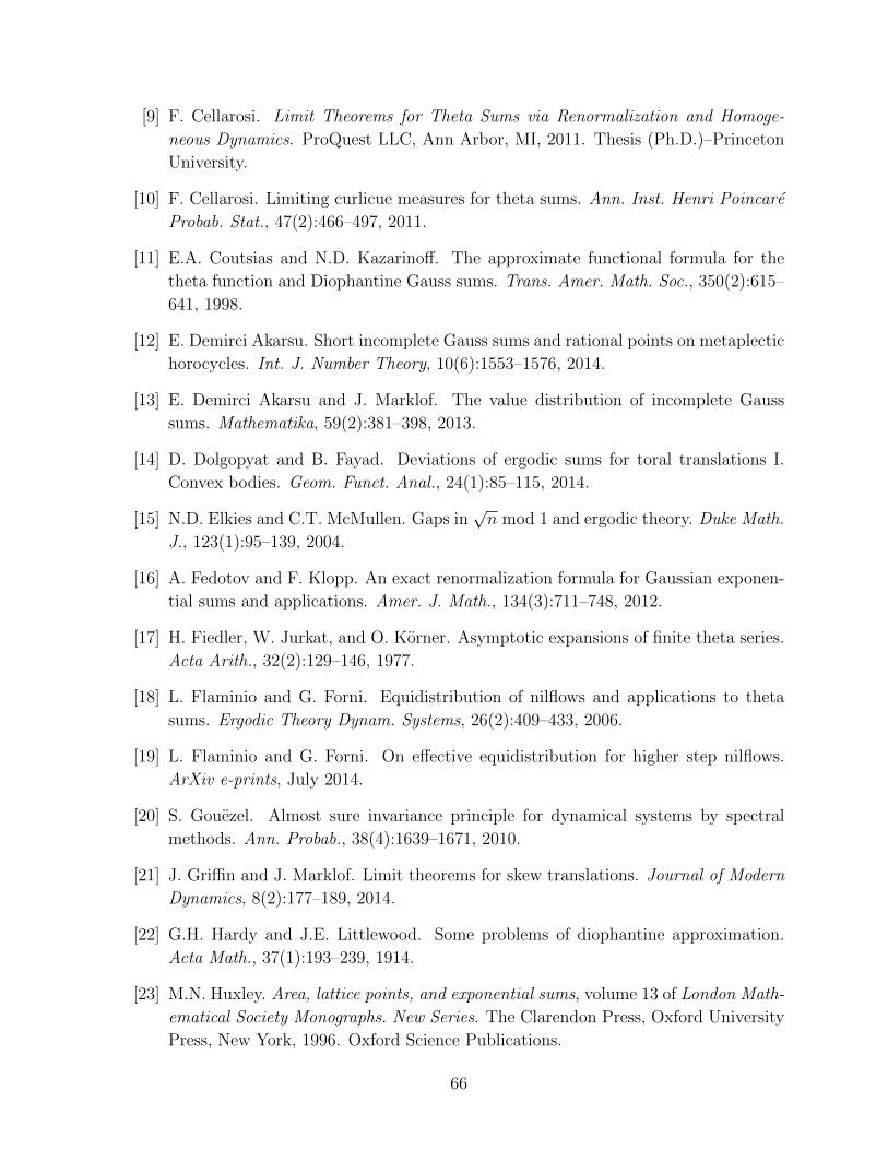
[9] F. Cellarosi. Limit Theorems for Theta Sums via Renormalization and Homoge-
neous Dynamics. ProQuest LLC, Ann Arbor, MI, 2011. Thesis (Ph.D.)–Princeton
University.
[10] F. Cellarosi. Limiting curlicue measures for theta sums. Ann. Inst. Henri Poincare
Probab. Stat., 47(2):466–497, 2011.
[11] E.A. Coutsias and N.D. Kazarinoff. The approximate functional formula for the
theta function and Diophantine Gauss sums. Trans. Amer. Math. Soc., 350(2):615–
641, 1998.
[12] E. Demirci Akarsu. Short incomplete Gauss sums and rational points on metaplectic
horocycles. Int. J. Number Theory, 10(6):1553–1576, 2014.
[13] E. Demirci Akarsu and J. Marklof. The value distribution of incomplete Gauss
sums. Mathematika, 59(2):381–398, 2013.
[14] D. Dolgopyat and B. Fayad. Deviations of ergodic sums for toral translations I.
Convex bodies. Geom. Funct. Anal., 24(1):85–115, 2014.
[15] N.D. Elkies and C.T. McMullen. Gaps in√n mod 1 and ergodic theory. Duke Math.
J., 123(1):95–139, 2004.
[16] A. Fedotov and F. Klopp. An exact renormalization formula for Gaussian exponen-
tial sums and applications. Amer. J. Math., 134(3):711–748, 2012.
[17] H. Fiedler, W. Jurkat, and O. Korner. Asymptotic expansions of finite theta series.
Acta Arith., 32(2):129–146, 1977.
[18] L. Flaminio and G. Forni. Equidistribution of nilflows and applications to theta
sums. Ergodic Theory Dynam. Systems, 26(2):409–433, 2006.
[19] L. Flaminio and G. Forni. On effective equidistribution for higher step nilflows.
ArXiv e-prints, July 2014.
[20] S. Gouezel. Almost sure invariance principle for dynamical systems by spectral
methods. Ann. Probab., 38(4):1639–1671, 2010.
[21] J. Griffin and J. Marklof. Limit theorems for skew translations. Journal of Modern
Dynamics, 8(2):177–189, 2014.
[22] G.H. Hardy and J.E. Littlewood. Some problems of diophantine approximation.
Acta Math., 37(1):193–239, 1914.
[23] M.N. Huxley. Area, lattice points, and exponential sums, volume 13 of London Math-
ematical Society Monographs. New Series. The Clarendon Press, Oxford University
Press, New York, 1996. Oxford Science Publications.
66
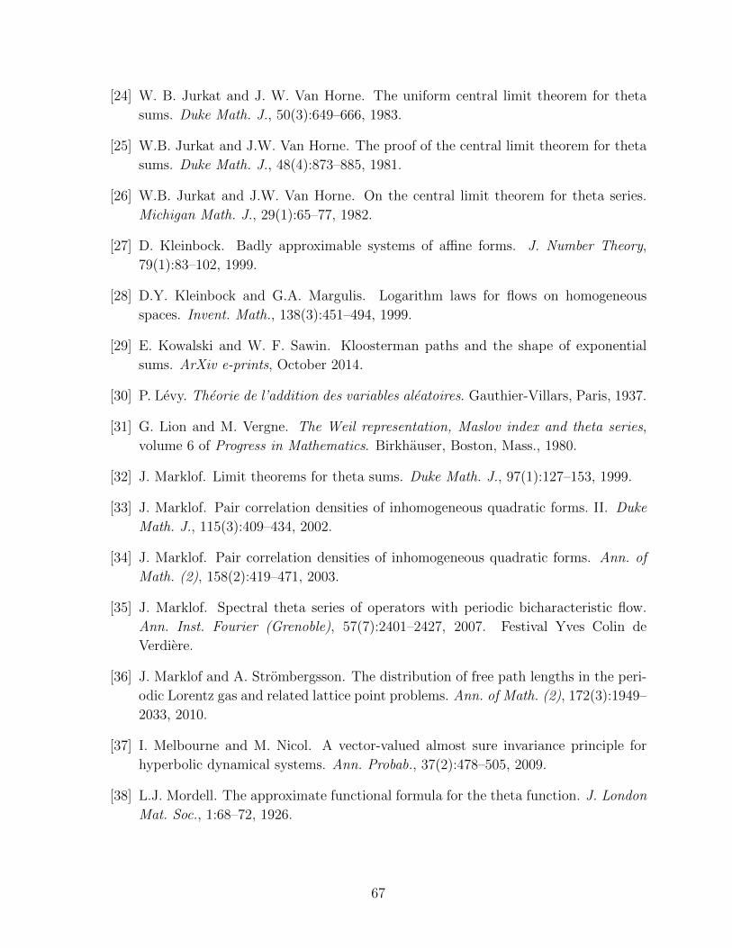
[24] W. B. Jurkat and J. W. Van Horne. The uniform central limit theorem for theta
sums. Duke Math. J., 50(3):649–666, 1983.
[25] W.B. Jurkat and J.W. Van Horne. The proof of the central limit theorem for theta
sums. Duke Math. J., 48(4):873–885, 1981.
[26] W.B. Jurkat and J.W. Van Horne. On the central limit theorem for theta series.
Michigan Math. J., 29(1):65–77, 1982.
[27] D. Kleinbock. Badly approximable systems of affine forms. J. Number Theory,
79(1):83–102, 1999.
[28] D.Y. Kleinbock and G.A. Margulis. Logarithm laws for flows on homogeneous
spaces. Invent. Math., 138(3):451–494, 1999.
[29] E. Kowalski and W. F. Sawin. Kloosterman paths and the shape of exponential
sums. ArXiv e-prints, October 2014.
[30] P. Levy. Theorie de l’addition des variables aleatoires. Gauthier-Villars, Paris, 1937.
[31] G. Lion and M. Vergne. The Weil representation, Maslov index and theta series,
volume 6 of Progress in Mathematics. Birkhauser, Boston, Mass., 1980.
[32] J. Marklof. Limit theorems for theta sums. Duke Math. J., 97(1):127–153, 1999.
[33] J. Marklof. Pair correlation densities of inhomogeneous quadratic forms. II. Duke
Math. J., 115(3):409–434, 2002.
[34] J. Marklof. Pair correlation densities of inhomogeneous quadratic forms. Ann. of
Math. (2), 158(2):419–471, 2003.
[35] J. Marklof. Spectral theta series of operators with periodic bicharacteristic flow.
Ann. Inst. Fourier (Grenoble), 57(7):2401–2427, 2007. Festival Yves Colin de
Verdiere.
[36] J. Marklof and A. Strombergsson. The distribution of free path lengths in the peri-
odic Lorentz gas and related lattice point problems. Ann. of Math. (2), 172(3):1949–
2033, 2010.
[37] I. Melbourne and M. Nicol. A vector-valued almost sure invariance principle for
hyperbolic dynamical systems. Ann. Probab., 37(2):478–505, 2009.
[38] L.J. Mordell. The approximate functional formula for the theta function. J. London
Mat. Soc., 1:68–72, 1926.
67
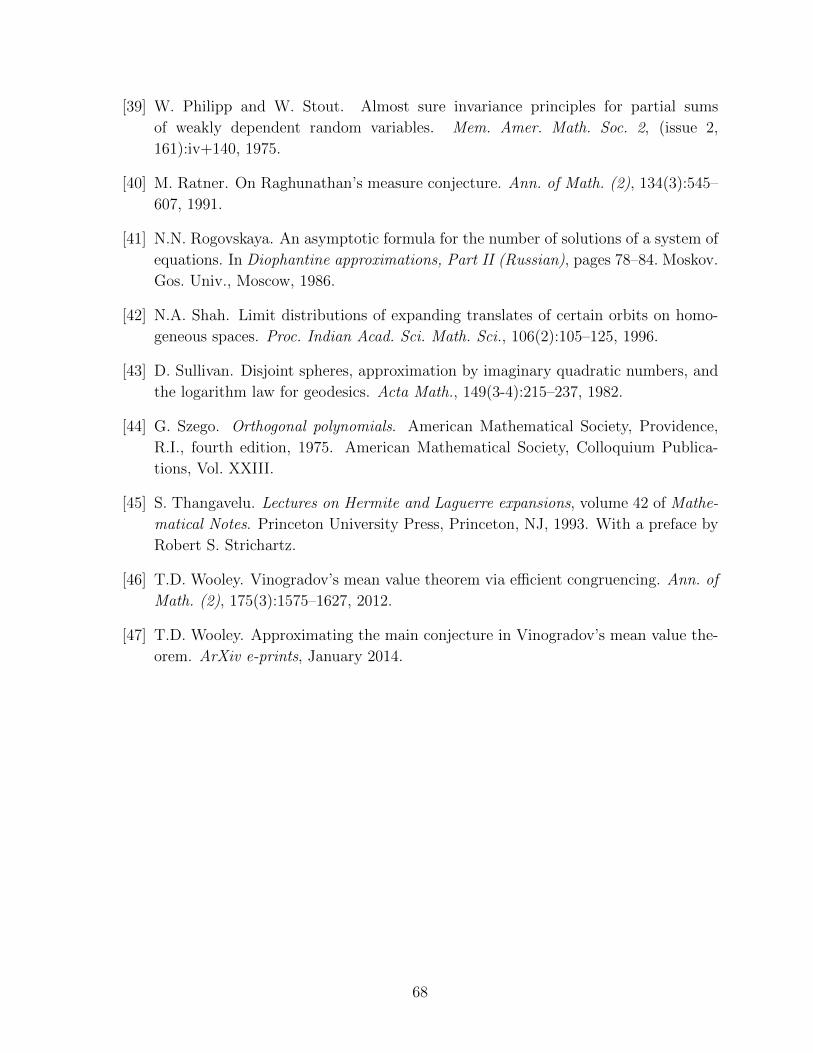
[39] W. Philipp and W. Stout. Almost sure invariance principles for partial sums
of weakly dependent random variables. Mem. Amer. Math. Soc. 2, (issue 2,
161):iv+140, 1975.
[40] M. Ratner. On Raghunathan’s measure conjecture. Ann. of Math. (2), 134(3):545–
607, 1991.
[41] N.N. Rogovskaya. An asymptotic formula for the number of solutions of a system of
equations. In Diophantine approximations, Part II (Russian), pages 78–84. Moskov.
Gos. Univ., Moscow, 1986.
[42] N.A. Shah. Limit distributions of expanding translates of certain orbits on homo-
geneous spaces. Proc. Indian Acad. Sci. Math. Sci., 106(2):105–125, 1996.
[43] D. Sullivan. Disjoint spheres, approximation by imaginary quadratic numbers, and
the logarithm law for geodesics. Acta Math., 149(3-4):215–237, 1982.
[44] G. Szego. Orthogonal polynomials. American Mathematical Society, Providence,
R.I., fourth edition, 1975. American Mathematical Society, Colloquium Publica-
tions, Vol. XXIII.
[45] S. Thangavelu. Lectures on Hermite and Laguerre expansions, volume 42 of Mathe-
matical Notes. Princeton University Press, Princeton, NJ, 1993. With a preface by
Robert S. Strichartz.
[46] T.D. Wooley. Vinogradov’s mean value theorem via efficient congruencing. Ann. of
Math. (2), 175(3):1575–1627, 2012.
[47] T.D. Wooley. Approximating the main conjecture in Vinogradov’s mean value the-
orem. ArXiv e-prints, January 2014.
68