Embed Size (px)
Citation preview
MULTI-SPACECRAFT STUDIES
OF PLASMA BOUNDARIES AT MARS
Thesis submitted for the degree of
Doctor of Philosophy
at the University of Leicester
by
Niklas Johan Theodor Edberg
Department of Physics and Astronomy
University of Leicester
September 2009

c© Niklas Johan Theodor Edberg, 2009
Abstract
Multi-spacecraft studies of plasma boundaries at Mars by NiklasJohan Theodor Edberg
We study the solar wind interaction with Mars and the location, shape,dynamics and controlling factors of the magnetic pileup boundary (MPB)and the bow shock (BS), which form as a result of this interaction, by usingsingle as well as two-spacecraft measurements.
By using Mars Global Surveyor (MGS) measurements we produce sta-tistical models of the shapes of the two boundaries. The influence on theboundaries from the crustal magnetic fields of Mars is also studied. We findthat the MPB is pushed to higher altitudes depending on the strength of theunderlying crustal fields while the BS is found at higher altitudes over theentire southern hemisphere of Mars, where the crustal fields are strongest.
By using the simultaneous measurements from Rosetta and Mars Express(MEX) we study the boundaries during high and low solar wind dynamicpressure. During low pressure, simultaneous two-spacecraft measurementsprovide leverage on the accuracy of the shape of the MPB and BS. Theirpreviously modelled shapes are found to be in agreement with the shapesderived from these two-point measurements. During high pressure, we ob-serve how the boundaries become asymmetric in their shapes, possibly dueto increased plasma outflow over one hemisphere, which lowers the plasmapressure on that side of the planet and results in an asymmetric shape.
By using MGS and MEX measurements we study the altitude of theboundaries as functions of solar wind dynamic pressure, solar EUV flux andcrustal magnetic field strength. We also examine the effect of the directionof the interplanetary magnetic field on the boundaries. We find that the dy-namic pressure, EUV flux and crustal magnetic fields are the main governingfactors of both the MPB and the BS.
iii
Acknowledgements
First of all I wish to thank my excellent supervisor Mark Lester for alwaysproviding useful input when needed but also for allowing me to roam freelywithin the realm of Mars and explore and study whatever I have found inter-esting. I am also very grateful to my second adviser Stan Cowley for manyquestions answered.
During the fall of 2007 I was given the opportunity to visit Anders Erikssonat the Swedish Institute of Space Physics in Uppsala, Sweden. For this I amalso very grateful. The result from that visit now constitutes a large fractionof this thesis. It also enabled me to catch my breath back in Sweden. Withnewly gathered strength from the homeland, I visited David Brain at theSpace Sciences Laboratory of UC Berkeley, USA, during the fall of 2008.I owe David many thanks for taking me in and enlightening me on manythings related to the science of Mars but also on many things related to thenon-science part of science. I would not have been able to finish my thesiswithout those two visits.
Furthermore, I wish to thank Ronan Modolo for always providing help andcomments. Stas Barabash and Markus Franz are greatly acknowledged forletting me use, and helping me getting started with, Mars Express ASPERA-3 data. The MGS MAG/ER and Rosetta RPC teams are also acknowledgedfor providing me with their data.
On a more personal note, I have had the fortunate opportunity to experiencea life in the UK for three years. Curries, tea breaks (coffee, really), pub trips,cricket, football, rugby, movie nights and poker nights as well as the wonderof wall-to-wall carpeting have truly fulfilled my time. For this I especiallywish to thank the many members of the RSPP group. Thanks to you all!
Finally, I also wish to thank Karin for sharing a life in science as well asin the real world.
iv

Declaration
The following papers have been produced during the time of these doctoralstudies, out of which the first four constitute the bulk of this Thesis
I. Edberg, N. J. T., Lester, M., Cowley, S. W. H. and Eriksson, A. I.,Statistical analysis of the location of the Martian magnetic pileupboundary and bow shock and the influence of crustal magnetic fields,J. Geophys. Res., 113, A08206, 2008
II. Edberg, N. J. T., Eriksson, A. I., Auster, U., Barabash, S., Boess-wetter, A., Carr, C. M., Cowley, S. W. H., Cupido, E., Franz, M.,Glassmeier, K.-H., Goldstein, R., Lester, M., Lundin, R., Modolo, R.,Nilsson, H., Richter, I., Samara, M. and Trotignon, J. G., Simultaneousmeasurements of Martian plasma boundaries by Rosetta and Mars Ex-press, Planet. Space Sci., 57, 1085-1096, doi:10.1016/j.pss.2008.10.016,2009
III. Edberg, N. J. T., Brain, D. A., Lester, M., Cowley, S. W. H., Modolo,R., Franz, M. and Barabash, S., Plasma boundary variability at Mars asobserved by Mars Global Surveyor and Mars Express, Ann. Geophys.,27, 3537-3550, 2009
IV. Edberg, N. J. T., Auster, U., Barabash, S., Boesswetter, A., Brain,D. A., Burch, J. L., Carr, C. M., Cowley, S. W. H., Cupido, E., Duru,F., Eriksson, A. I., Franz, M., Glassmeier, K.-H., Goldstein, R., Lester,M., Lundin, R., Modolo, R., Nilsson, H., Richter, I., Samara, M. andTrotignon, J. G., Rosetta and Mars Express observations of the in-fluence of high solar wind dynamic pressure on the Martian plasmaenvironment, Submitted to Ann. Geophys., 2009
V. Boesswetter, A., Auster, U., Richter, I., Franz, M., Langlais, B., Si-mon, S., Motschmann, U., Glassmeier, K.-H., Edberg, N. J. T., andLundin, R., Rosetta swing-by at Mars - an analysis of the ROMAP
v
measurements in comparison with results of 3d multi-ion hybrid sim-ulations and MEX/ASPERA-3 data, Ann. Geophys., 27, 2383-2398,2009
VI. Odzimek, A., Clausen, L. B. N., Kanawade, V., Cnossen, I., Edberg,N. J. T., Faedi, F., Del Moro, A., Ural, U., Byckling, K., Krza-czkowski, P., Iwanski, R., Struzik, P., Pajek, M., and Gajda, W.,SPARTAN Sprite-Watch Campaign 2007, In: 15th Young ScientistsConference on Astronomy and Space Physics. Proceedings of Con-tributed Papers, edited by V.Ya. Choliy and G. Ivashchenko, Logos,Kyiv, pp. 64-67, 2009.
VII. Iwanski, R., Odzimek, A., Clausen, L.B.N., Kanawade, V., Cnossen,I., Edberg, N. J. T., Meteorological study of the first observation ofred sprites from Poland, Acta. Geophysica, 57-3, 760-777, 2009.
VIII. Eriksson, A. I., Gill, R., Wahlund, J.-E., Andre, M., Malkki, A., Ly-bekk, B., Pedersen, A., Holtet, J. A., Blomberg, L. G., and Edberg,N. J. T., RPC-LAP: The Langmuir probe instrument of the Rosettaplasma consortium, In Rosetta: ESA’s mission to the origin of thesolar system, eds. R. Schulz, C. Alexander, H. Boehnhardt and K.-H. Glassmeier, pp. 435-447. Springer, ISBN: 97 8-0-387-77517-3.doi:10.1007/978-0-387-77518-0 15 4, 2009
Contents
1 Introduction 11.1 Space plasma physics . . . . . . . . . . . . . . . . . . . . . . . 2
1.1.1 Magnetohydrodynamics . . . . . . . . . . . . . . . . . 21.1.2 Frozen-in flow . . . . . . . . . . . . . . . . . . . . . . . 21.1.3 Parker spiral . . . . . . . . . . . . . . . . . . . . . . . . 41.1.4 Gyro-motion and E× B - drift . . . . . . . . . . . . . 41.1.5 Debye length . . . . . . . . . . . . . . . . . . . . . . . 71.1.6 Thermal, kinetic and magnetic pressure . . . . . . . . . 8
1.2 The planet Mars . . . . . . . . . . . . . . . . . . . . . . . . . 91.3 The solar wind interaction with Mars . . . . . . . . . . . . . . 11
1.3.1 The ionosphere and the photo-electron boundary . . . 111.3.2 The bow shock and magnetic pileup boundary . . . . . 141.3.3 The tail region . . . . . . . . . . . . . . . . . . . . . . 211.3.4 Crustal magnetic fields . . . . . . . . . . . . . . . . . . 221.3.5 Global models of the Martian plasma environment . . . 251.3.6 Erosion of the atmosphere . . . . . . . . . . . . . . . . 26
2 Instrumentation 322.1 Mars Global Surveyor: magnetometer and electron reflectometer 322.2 Mars Express: ASPERA-3 and MARSIS . . . . . . . . . . . . 332.3 Rosetta: The Rosetta Plasma Consortium . . . . . . . . . . . 372.4 Moments from ion and electron measurements . . . . . . . . . 392.5 Rosetta and Mars Express density cross-calibration . . . . . . 41
3 Mars Global Surveyor measurements of the influence of thecrustal magnetic fields 463.1 Introduction . . . . . . . . . . . . . . . . . . . . . . . . . . . . 463.2 Data analysis . . . . . . . . . . . . . . . . . . . . . . . . . . . 47
3.2.1 Shape of bow shock and magnetic pileup boundary . . 503.2.2 The influence of crustal magnetic fields . . . . . . . . . 54
vii
3.2.3 Magnetic field strength at the magnetic pileup boundary 613.3 Summary and conclusions . . . . . . . . . . . . . . . . . . . . 64
4 Rosetta and Mars Express simultaneous measurements of theeffects of low and high solar wind pressure 684.1 Introduction . . . . . . . . . . . . . . . . . . . . . . . . . . . . 694.2 Simultaneous observations during low solar wind pressure . . . 69
4.2.1 Dayside bow shock crossing . . . . . . . . . . . . . . . 714.2.2 Dayside MPB and PEB crossings . . . . . . . . . . . . 724.2.3 Flank MPB crossing . . . . . . . . . . . . . . . . . . . 754.2.4 Flank magnetosheath and bow shock crossings . . . . . 774.2.5 Mars Express observations . . . . . . . . . . . . . . . . 79
4.3 Shape and location of the plasma boundaries . . . . . . . . . . 824.4 Simultaneous observations during high pressure solar wind . . 86
4.4.1 Plasma boundary asymmetries . . . . . . . . . . . . . . 884.4.2 Cause of the asymmetries . . . . . . . . . . . . . . . . 954.4.3 Ion outflow and exosphere asymmetry . . . . . . . . . . 99
4.5 Boundary asymmetry linked to the ionospheric outflow . . . . 1034.6 Summary and conclusions . . . . . . . . . . . . . . . . . . . . 107
5 Mars Express and Mars Global Surveyor measurements 1115.1 Introduction . . . . . . . . . . . . . . . . . . . . . . . . . . . . 1115.2 Measurements of and proxies for the dynamic pressure, IMF
direction and solar EUV flux . . . . . . . . . . . . . . . . . . . 1125.3 Mars Express and Mars Global Surveyor observations . . . . . 1155.4 Case studies with simultaneous measurements . . . . . . . . . 1165.5 Statistical studies with simultaneous measurements . . . . . . 124
5.5.1 Influence of the solar wind dynamic pressure . . . . . . 1245.5.2 Influence of the IMF direction . . . . . . . . . . . . . . 128
5.6 Influence of the crustal magnetic fields . . . . . . . . . . . . . 1315.7 Influence of the solar EUV flux . . . . . . . . . . . . . . . . . 1355.8 Summary and conclusions . . . . . . . . . . . . . . . . . . . . 136
6 Conclusions & future work 1416.1 Conclusions . . . . . . . . . . . . . . . . . . . . . . . . . . . . 1416.2 Future work . . . . . . . . . . . . . . . . . . . . . . . . . . . . 144
Chapter 1Introduction
The Sun continuously emits plasma into space which forms the solar wind.
The solar wind consists of mainly hydrogen and helium ions and electrons
which propagate radially outward from the Sun. It continues to propa-
gate outward into the solar system until it either encounters the interstellar
medium at the edge of the solar system or it encounters a planetary body.
It is this solar wind’s interaction with planet Mars that is the topic of this
Thesis. The average density of the solar wind is on the order of ∼2 cm−3 at
Mars and the average speed on the order of ∼400 km s−1. The Sun also pos-
sesses a magnetic field which is convected outward by the solar wind forming
the interplanetary magnetic field (IMF), which at Mars is on the order of ∼3
nT.
In this Chapter we will first describe the basic physics of the solar wind
plasma and the general properties of the planet Mars before we summarize
some of the key features which arise from the solar wind interaction with
Mars.
1
CHAPTER 1. INTRODUCTION 2
1.1 Space plasma physics
1.1.1 Magnetohydrodynamics
The equations that describe the properties of the particles, currents and elec-
tric and magnetic fields that exist in the magnetised solar wind plasma are
Maxwell’s equations together with the equations for conservation of mass,
momentum and energy in the so called magnetohydrodynamic (MHD) ap-
proximation. The plasma is then treated as a fluid and kinetic phenomena
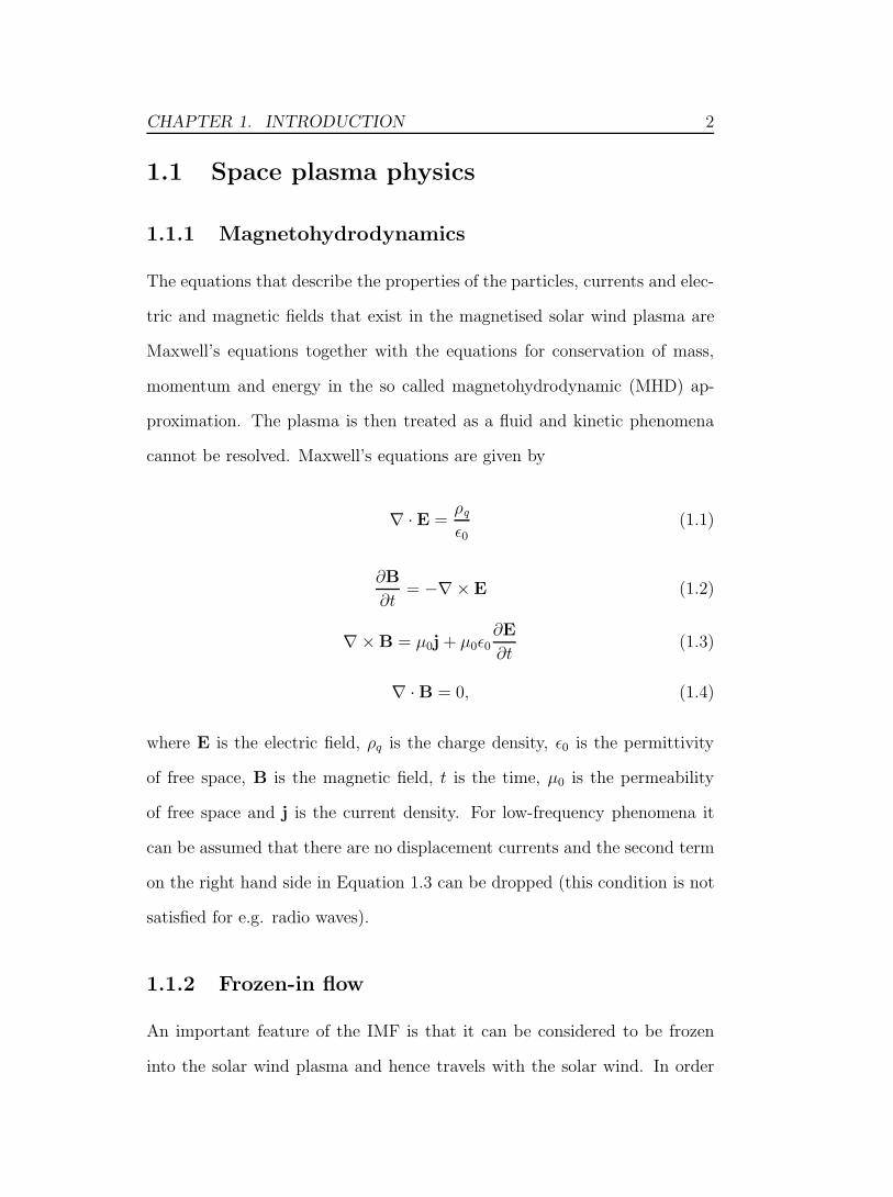
cannot be resolved. Maxwell’s equations are given by
∇ · E =ρq
ε0(1.1)
∂B
∂t= −∇×E (1.2)
∇×B = μ0j + μ0ε0∂E
∂t(1.3)
∇ · B = 0, (1.4)
where E is the electric field, ρq is the charge density, ε0 is the permittivity
of free space, B is the magnetic field, t is the time, μ0 is the permeability
of free space and j is the current density. For low-frequency phenomena it
can be assumed that there are no displacement currents and the second term
on the right hand side in Equation 1.3 can be dropped (this condition is not
satisfied for e.g. radio waves).
1.1.2 Frozen-in flow
An important feature of the IMF is that it can be considered to be frozen
into the solar wind plasma and hence travels with the solar wind. In order
CHAPTER 1. INTRODUCTION 3
to explain this we need to first consider Ampere’s law
j =∇× B
μ0
, (1.5)
and conclude that the size of the current density is on the order of
j ∼ B
μ0L, (1.6)
where L is the scale length on which the magnetic field varies significantly.
Ohm’s law gives
E = −v × B + j/σ, (1.7)
where v is the bulk velocity of the plasma and σ is the conductivity, and by
taking the curl of this and using Faraday’s law (Equation 1.2) and Ampere’s
law (Equation 1.3) we obtain the induction equation
∂B
∂t= ∇× (v ×B) + η∇2B, (1.8)
where η = 1μ0σ
. The first term on the right hand side of Equation 1.8 describes
convection of B with v (’frozen-in’ flow) and the second term is the magnetic
diffusion. The dimensionless ratio of the first and second term is the magnetic
Reynolds number
Rm =vL
η= μ0σvL, (1.9)
which is a very large number (∼ 106 − 1012) for most situations in the solar
wind. On scales L such that Rm is very large then Equation 1.8 reduces to
∂B
∂t∼ ∇× (v × B), (1.10)
CHAPTER 1. INTRODUCTION 4
and the magnetic field can therefore be considered to be frozen into the
plasma. Ohm’s law (Equation 1.7) then reduces to
E + v × B = 0, (1.11)
where is E sometimes called the convective electric field or motional electric
field (note that the same result is obtained if the conductivity in equation 1.7
goes to infinity). As a consequence of Equation 1.10, the solar wind particles
that are fixed within a magnetic flux tube at a certain time will always stay
within that flux tube, as long as the frozen-in condition holds (e.g. across
current sheets).
1.1.3 Parker spiral
Since the IMF is connected to the rotating Sun the magnetic field forms a
spiral shape in interplanetary space. The magnetic field continuously prop-
agates radially outward, frozen into the solar wind while still connected to
the source region on the Sun, which rotates (with a revolution period of
∼24-27 days, depending on latitude). This results in a spiral shape of the
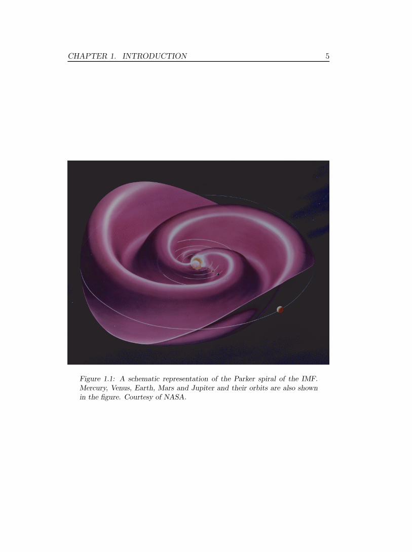
IMF known as the Parker spiral. The Parker spiral shape of the IMF is
shown schematically in Figure 1.1. In particular, this means that at Mars
the IMF is normally oriented in the ecliptic plane with an angle of 57◦ from
the Sun-Mars line.
1.1.4 Gyro-motion and E × B - drift
There are many drifts and motions of plasma particles in the presence of an
electric field E and a magnetic field B in space. We will not describe them
CHAPTER 1. INTRODUCTION 5
Figure 1.1: A schematic representation of the Parker spiral of the IMF.Mercury, Venus, Earth, Mars and Jupiter and their orbits are also shownin the figure. Courtesy of NASA.
CHAPTER 1. INTRODUCTION 6
all but rather focus on two of them in the following Section.
The Lorentz forces that act upon a single particle with charge q and
velocity v are
F = q(E + v × B). (1.12)
Applying this to Newton’s second law
F = ma, (1.13)
where m is the mass and a is the acceleration gives
mdv
dt= q(E + v ×B). (1.14)
Solving the above differential equation in the direction parallel and perpen-
dicular to the magnetic field, gives rise to the two characteristic movements.
First, the perpendicular components results in a motion where the ions and
electrons gyrate around the magnetic field lines with a gyro frequency
ωc =qB
m, (1.15)
and a gyro radius
rc =mv⊥qB
, (1.16)
where v⊥ is the velocity component perpendicular to the magnetic field.
The second movement comes from the parallel components of Equation
1.14. The particles are accelerated by the electric field, in the direction of the
electric field for the positively charged ions and in the opposite direction of the
electric field for the negatively charged electrons. During one complete gyro-

CHAPTER 1. INTRODUCTION 7
cycle the magnetic force, always being perpendicular to the motion of the
particle, averages out. But the electric force is always in the same direction.
This leads to the gyro-motion of the particle not forming a perfect circle.
On one half of each gyration is the particle accelerated by the electric field
and on the other half is it being decelerated such that the particle travels a
longer distance on one half than the other. This leads to a drift motion of
the particles in a direction perpendicular to both E and B
vE×B =E× B
B2. (1.17)
Ions and electrons, with opposite charge, gyrate in different directions while
their drifts, in a collisionless plasma, are in the same direction independent
of charge q and mass m.
1.1.5 Debye length
In a plasma, a single ion whose electrostatic potential is
Φ(r) =q
4πε0r, (1.18)
where r is the radial distance, will attract electrons while ions, with their
larger masses, will be only somewhat repelled. This will change the potential
to
Φ(r) = qe−r/λD/(4πε0r), (1.19)
where
λD =
(εkT
nq2
)1/2
(1.20)
CHAPTER 1. INTRODUCTION 8
is the Debye length, T is the temperature and k is Boltzmann’s constant.
In a cloud of plasma particles where a Maxwellian distribution of the energy
of the particles can be assumed we get collective behaviour of the plasma
rather than a collection of individual particles. The Debye sphere is then
a shielding sphere of radius λD outside of which charges and electric fields
are screened off. The Debye length is a useful quantity since it is a measure
of the length over which charge separation can occur and the distance over
which a charge separation influence its surroundings. In the solar wind this
quantity is typically on the order of ∼ 10 m. The charge-density separation
between electrons and ions also gives rise to an oscillation of the particles
with a plasma frequency
ωps =
(nq2
ε0m
)1/2
. (1.21)
1.1.6 Thermal, kinetic and magnetic pressure
Finally, there are three types of pressure associated with the solar wind
plasma. First, the thermal gas pressure is
pTh = nekTe + nikTi, (1.22)
where ni and ne are the ion and electron densities and Ti and Te the ion and
electron temperatures, respectively. The magnetic pressure is
pB =B2
2μ0(1.23)
and the dynamic pressure
pDyn = ρv2, (1.24)
CHAPTER 1. INTRODUCTION 9
where ρ is the mass density.
1.2 The planet Mars
The planet Mars is the fourth planet from the Sun and the second smallest
of all planets in the solar system with a radius of 3397 km and a mass of
6.4 · 1023 kg (∼ 11% of the Earth’s mass). Consequently, the gravitational
acceleration on Mars is 3.72 m s−2. The orbit of Mars is more elliptic than
the Earth’s orbit and its distance from the Sun varies between 1.37 AU and
1.67 AU (1 AU = 1.5·108 km = the average Sun-Earth distance). The orbital
period (a Martian year) is 687 days and a revolution period (a Martian day
or a ‘sol’) is 24h 40 min making a Martian year 668 sols. Mars’s revolution
axis is tilted by 25◦, which is similar to the Earth’s tilt of 23◦, and hence
there are spring, summer, autumn, and winter seasons on Mars as well.
The atmosphere of Mars is very different from that at Earth. The surface
pressure is only 0.007 bars and the main constituents are carbon dioxide,
CO2 (95.3%), nitrogen, N2 (2.7%) and argon, Ar (1.6%). There is very little
oxygen, O2 (0.13%) and even less water, H20 (0.03%). Clouds can form on
Mars and even snowfall has been detected by the recent Phoenix Mars lander
mission. The polar regions are also covered by water ice and carbon dioxide
ice, which sublimates in the summer and freezes again in the winter.
Mars does not possess a global intrinsic dipole-like magnetic field like
the Earth but it does have strong crustal magnetic sources, which will be
described in more detail in Section 1.3.4.
Over the past 50 years, there have been more than 40 attempts to send
spacecraft missions to Mars. Only about 50% of these reached Mars and
CHAPTER 1. INTRODUCTION 10
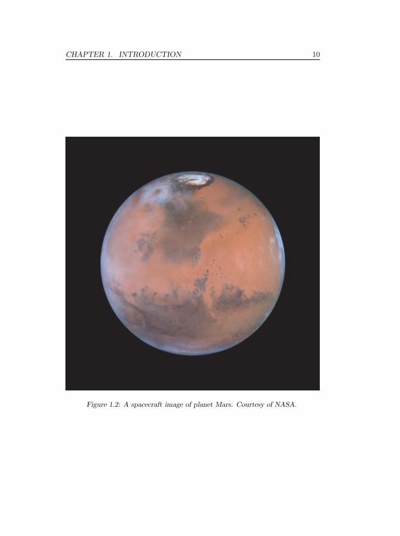
Figure 1.2: A spacecraft image of planet Mars. Courtesy of NASA.
CHAPTER 1. INTRODUCTION 11
could be labelled successful and not all of these successful missions carried
plasma instruments. Out of the ones that did carry plasma instruments
we should mention Phobos 2 (arrived 1989), Mars Global Surveyor (MGS)
(arrived 1997), Mars Express (MEX) (arrived 2003) and Rosetta (swingby
2007), which will all be referred to extensively in this Thesis.
1.3 The solar wind interaction with Mars
When the solar wind encounters a planet or any other major body in the
solar system a complex interaction region is formed. This interaction region
is characterized by various different plasma regimes with distinct boundaries.
The solar wind interaction with celestial bodies is usually divided into three
cases: interaction with a magnetised body, as for the case of Earth and the gas
giant planets such as Jupiter and Saturn, interaction with a non-magnetised
body with no significant atmosphere, as for the Moon and asteroids, and
finally, interaction with a non-magnetised planet with an atmosphere, as for
Venus, comets and Mars.
1.3.1 The ionosphere and the photo-electron boundary
The effective obstacle to the solar wind at Mars is the ionosphere. We will
therefore first describe the features of the ionosphere before we describe its
interaction with the solar wind.
The ionosphere is a thick (∼ 200-300 km) region in the upper regions of
the neutral atmosphere where planetary molecules have been ionised to form
a mixture of some ions and electrons and lots of neutral gas. In situ measure-
ments of the Martian ionosphere have only been performed by the two Viking
CHAPTER 1. INTRODUCTION 12
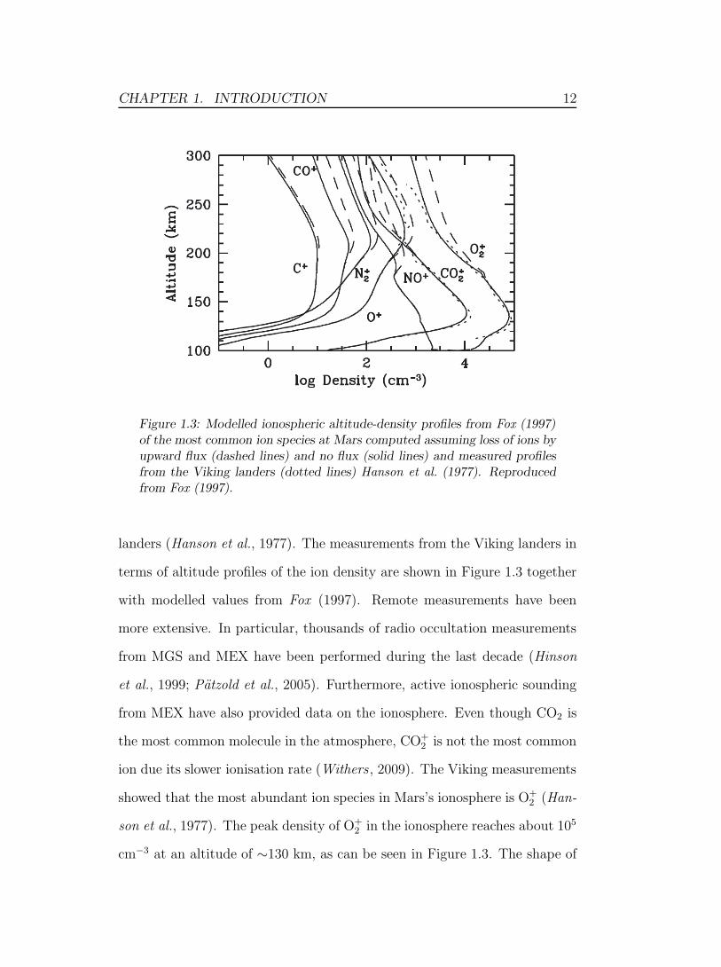
Figure 1.3: Modelled ionospheric altitude-density profiles from Fox (1997)of the most common ion species at Mars computed assuming loss of ions byupward flux (dashed lines) and no flux (solid lines) and measured profilesfrom the Viking landers (dotted lines) Hanson et al. (1977). Reproducedfrom Fox (1997).
landers (Hanson et al., 1977). The measurements from the Viking landers in
terms of altitude profiles of the ion density are shown in Figure 1.3 together
with modelled values from Fox (1997). Remote measurements have been
more extensive. In particular, thousands of radio occultation measurements
from MGS and MEX have been performed during the last decade (Hinson
et al., 1999; Patzold et al., 2005). Furthermore, active ionospheric sounding
from MEX have also provided data on the ionosphere. Even though CO2 is
the most common molecule in the atmosphere, CO+2 is not the most common
ion due its slower ionisation rate (Withers , 2009). The Viking measurements
showed that the most abundant ion species in Mars’s ionosphere is O+2 (Han-
son et al., 1977). The peak density of O+2 in the ionosphere reaches about 105
cm−3 at an altitude of ∼130 km, as can be seen in Figure 1.3. The shape of

CHAPTER 1. INTRODUCTION 13
the altitude profiles are in reasonable agreement with what is expected from
the commonly used Chapman theory (Chapman, 1931a,b). The density in-
creases exponentially with decreasing altitude up to a point, and the density
of the main peak falls off with solar zenith angle (SZA) (Morgan et al., 2008;
Withers , 2009).
The main ionisation source on the dayside of Mars is photoionisation
by solar EUV photons which creates the main peak in the altitude profiles.
Below the main peak, electron-impact processes and X-ray photons become
more important and form a second layer (Withers , 2009). At even lower al-
titudes, meteoritic impacts can create a sporadic third layer (Patzold et al.,
2005). Toward the nightside the ionosphere becomes more and more con-
trolled by electron transport processes from the dayside but since the Mar-
tian ionosphere is generally magnetized this transport is rather weak (Nagy
et al., 2004). This is, however, an area that is poorly investigated and re-
quires further study. Factors that have been shown to affect the properties
of the ionosphere include crustal magnetic fields (Withers et al., 2005) and
solar energetic particles (Espley et al., 2007).
At Venus, for instance, the transition into the ionosphere is usually very
clear. A sharp increase (on inbound passes) in the ion and electron density,
called the ionopause, is clearly visible in spacecraft data. At Mars, this tran-
sition is much more smeared out and the term ‘ionopause’ is not really ade-
quate. There is no sharp transition into an ionosphere. A related boundary
has, however, been observed by the electron spectrometers onboard MGS and
MEX. This is not an ionopause in the normal sense but a boundary where a
strong peak in the observed electron spectrum from photoionised CO2 starts
to appear at energies of ∼ 20-30 eV. This boundary has been labelled the
CHAPTER 1. INTRODUCTION 14
photo-electron boundary (PEB) (Frahm et al., 2006). The PEB is located at
an altitude of about 250 km on the dayside of Mars and extends to at least 10
000 km downstream of Mars (where the farthest downstream measurements
from MEX are made) in a cylindrical shape of approximately the planetary
radius (Frahm et al., 2006). The PEB was, however, also noted in earlier
data from MGS (Mitchell et al., 2001) but due to the low energy resolution
of the electron spectrometer the nature of this boundary remained somewhat
unclear until the arrival of MEX (Frahm et al., 2006).
1.3.2 The bow shock and magnetic pileup boundary
The solar wind interaction with Mars leads to the formation of plasma re-
gions with distinct boundaries which are the main topic in this Thesis. These
boundaries form at altitudes of ∼ 1-2 RM on the dayside and at even higher
altitudes toward the nightside. For the case of an interaction with an unmag-
netized body with an atmosphere, such as Mars, the main three boundaries
are the bow shock (BS), the magnetic pileup boundary (MPB) and the photo-
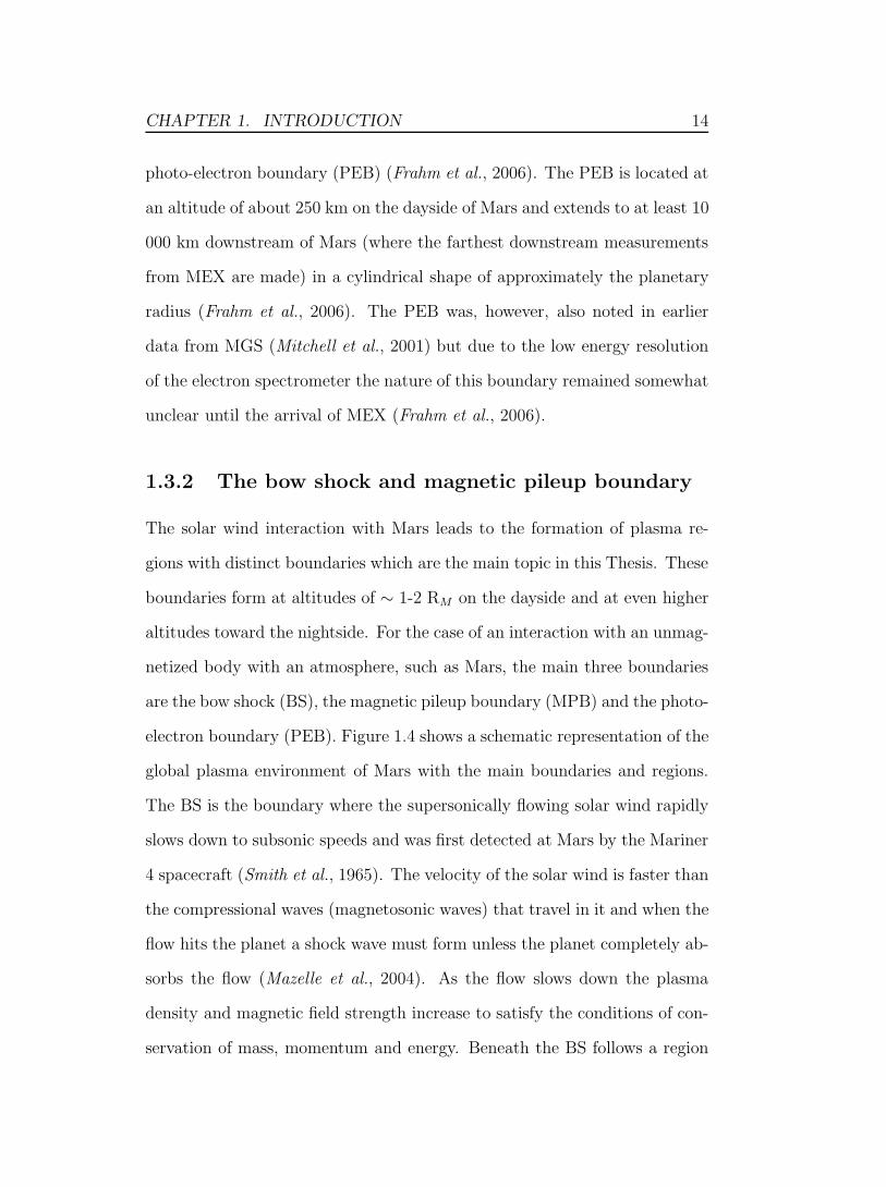
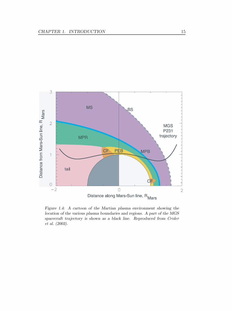
electron boundary (PEB). Figure 1.4 shows a schematic representation of the
global plasma environment of Mars with the main boundaries and regions.
The BS is the boundary where the supersonically flowing solar wind rapidly
slows down to subsonic speeds and was first detected at Mars by the Mariner
4 spacecraft (Smith et al., 1965). The velocity of the solar wind is faster than
the compressional waves (magnetosonic waves) that travel in it and when the
flow hits the planet a shock wave must form unless the planet completely ab-
sorbs the flow (Mazelle et al., 2004). As the flow slows down the plasma
density and magnetic field strength increase to satisfy the conditions of con-
servation of mass, momentum and energy. Beneath the BS follows a region
CHAPTER 1. INTRODUCTION 15
Figure 1.4: A cartoon of the Martian plasma environment showing thelocation of the various plasma boundaries and regions. A part of the MGSspacecraft trajectory is shown as a black line. Reproduced from Crideret al. (2003).
CHAPTER 1. INTRODUCTION 16
of shocked solar wind called the magnetosheath, characterized by heated and
more turbulent solar wind plasma. The Mach number (sonif, magnetosonic
and Alfenic) in the solar wind determines how much deceleration and heating
takes place at the BS (Mazelle et al., 2004). The Martian exosphere, which
is the uppermost region around Mars where upward travelling molecules can
either escape into space if the velocity is high enough or be pulled back to the
planet by the gravity, is rather extended outside the BS compared to Venus
and Earth due to the low gravity on Mars. This is important as it affects
the amount of waves upstream of the BS (Mazelle et al., 2004).
The magnetosheath, downstream of the BS, is separated from the plan-
etary plasma and the magnetic pileup region (MPR) by the MPB. At the
MPB the IMF starts to pile up, since it cannot penetrate efficiently into
the ionosphere, and drapes around the planet before it slips past around the
sides of the obstacle (Nagy et al., 2004). This boundary has been named
the planetopause, magnetopause, protonopause or ion-composition bound-
ary depending on which spacecraft sampled it and which instruments it used
to measure the characteristics of the boundary (Trotignon et al., 2006). The
plasma population differs across this boundary, with mainly solar wind ions
in the magnetosheath and planetary ions in the MPR.
Several spacecraft have sampled the Martian plasma environment and the
amount of data has increased significantly during the last decade (from 1997)
with the measurements from MGS and MEX. Slavin and Holzer (1981) pre-
sented early work on the shape of the BS at Mars using data from the early
‘Mars’ series of spacecraft. The BS has also been studied using Phobos 2
measurements by Schwingenschuh et al. (1990) and Trotignon et al. (1991,
1993), while the MPB has been studied, referred to as the magnetopause
CHAPTER 1. INTRODUCTION 17
by Lundin et al. (1990), the planetopause by Trotignon et al. (1996) and
the protonopause by Sauer et al. (1992) among others. The instrumentation
on board Phobos 2 was more extensive than on MGS, but Phobos 2 did not
complete as many orbits and did not provide data with such good spatial cov-
erage as MGS. Also, Phobos 2 had its periapsis at 850 km which was too high
to decisively determine the nature of the dayside MPB. The Martian plasma
environment could therefore be more extensively studied with the MGS mis-
sion. Phobos 2 is the only spacecraft which have carried an instrument for
studying electric fields at Mars, which, for instance, showed how the plasma
turbulence increased when the BS was crossed and the magnetosheath was
entered (Grard et al., 1989).
The coordinate system that has been used to examine the location of the
boundaries is the Mars solar orbital (MSO) system, where the x-axis points
toward the Sun, the y-axis points approximately opposite to Mars’ orbital
motion, and the z-axis is directed parallel to the orbital angular momentum
vector of Mars (Slavin and Holzer , 1981). This coordinate system is rotated
by 4◦ about the z-axis to account for the aberration of the solar wind flow
direction by the planetary orbital motion. The method used to determine
the shape of the two boundaries developed by Slavin and Holzer (1981) has
been to fit a conic section
r =L
1 + εcos(θ)(1.25)
to the crossings, where r and θ are polar coordinates with origin at X0
referenced to the x-axis, and L and ε are the eccentricity and semi-latus
rectum, respectively (Slavin and Holzer , 1981).
CHAPTER 1. INTRODUCTION 18
Since the arrival of MGS the shape and structure of both the MPB and
BS have been studied in more detail. Vignes et al. (2000) published results
on the boundary shapes using data from the first year of the pre-mapping
phase of the mission. The average position of the boundaries could be deter-
mined with more accuracy using the MGS measurements due to the many
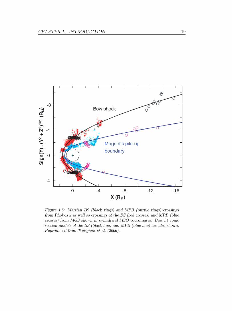
more crossings than obtained by Phobos 2. Trotignon et al. (2006) combined
MGS and Phobos 2 data to produce a more realistic boundary shape farther
downstream. The models of the BS and MPB from the study by Trotignon
et al. (2006) are shown in Figure 1.5. Bertucci et al. (2005) on the other hand
used a minimum variance technique to estimate the local normal vector at
each MPB crossing to confirm the shape derived by Vignes et al. (2000). Due
to the orbit configuration of MGS, no crossings of the MPB were observed
below a SZA of ∼20◦. This introduced an error in the fitting of a conic
section to the boundary when using MGS boundary crossings. The standoff
distance at the subsolar point (SZA = 0◦) of the empirical models were in
fact larger than the distance at SZA = 45◦ which does not seem reasonable.
MEX on the other hand, could later on sample the boundary at lower SZAs
and hence correct the problem.
There are a number of factors controlling the location of the MPB and BS.
Rosenbauer et al. (1994) provided first experimental evidence, using Phobos
2 data, that the magnetic pressure in the Martian tail balanced the upstream
solar wind dynamic pressure. Verigin et al. (1993) used the same data set
to study the influence of the upstream dynamic pressure and magnetic field
strength on the boundary locations. Crider et al. (2003) used MGS data and
studied the variation of the magnetic field strength inside the MPB in the
MPR and stated that this could be used as a proxy for upstream dynamic
CHAPTER 1. INTRODUCTION 19
Figure 1.5: Martian BS (black rings) and MPB (purple rings) crossingsfrom Phobos 2 as well as crossings of the BS (red crosses) and MPB (bluecrosses) from MGS shown in cylindrical MSO coordinates. Best fit conicsection models of the BS (black line) and MPB (blue line) are also shown.Reproduced from Trotignon et al. (2006).
CHAPTER 1. INTRODUCTION 20
pressure. The dynamic pressure as measured upstream of the planet was
confirmed, by MEX measurements, to be one of the controlling factors of the
location of the MPB when the magnetic pressure of the piled up field in the
MPR was shown to balance the dynamic pressure of the solar wind (Dubinin
et al., 2006). In between the MPR and the solar wind is the magnetosheath
where the thermal pressure balances the magnetic pressure from the inside
and the dynamic pressure from the outside (Dubinin et al., 2008a). The large
data set from MEX enables a further statistical study of the dependence on
upstream solar wind dynamic pressure on the plasma boundaries which is
one of the topics in this Thesis (see Chapter 5).
The 11-year solar cycle dependence has proved to be weak since the lo-
cations of the MPB and BS were not found to be significantly different in
Phobos 2 and MGS measurements which sampled the boundary in different
parts of the solar cycle. Phobos 2 sampled the boundaries during the in-
creasing phase of the solar cycle and MGS sampled the boundaries during
solar minimum. MEX started sampling the boundaries during the declining
phase of the solar cycle as well but will have the opportunity to sample them
during solar maximum if it stays alive for another 5 years or so.
The effect of the IMF orientation has been studied and shown to influence
the BS location (Vignes et al., 2002). The explanation for this is that the IMF
direction determines the direction of the convective electric field (Equation
1.11), which causes magnetosheath ions to move in the direction of the electric
field and electrons the opposite way, creating an asymmetry which also causes
the shape of the boundary to become asymmetric. However, in the study by
Vignes et al. (2002) only a small subset of the crossings were used when the
IMF was steady. This decreased the number of data points significantly.

CHAPTER 1. INTRODUCTION 21
As stated above, there are a number of factors that potentially influence
the position and shape of the plasma boundaries, such as solar wind dynamic
pressure, IMF direction and thermal pressure inside the BS. Added to that
list are the crustal magnetic fields of Mars, which will be introduced in Section
1.3.4. All these factors are more or less important, which will be further
investigated in Chapter 5, and when they mix with each other it becomes
challenging to determine the cause of the dynamics of the boundaries, which
will be discussed in Chapter 4.
1.3.3 The tail region
As the IMF piles up at the MPB, the field lines drape around the planet
to form the induced tail and central plasma sheet behind the planet. The
draped field lines, which are orientated according to the IMF direction on the
dayside (Brain et al., 2006), form two lobes of oppositely directed orientation
when they meet again behind the planet and a Harris current sheet can form
(Halekas et al., 2006; Halekas and Brain, 2009). The plasma sheet is oriented
according to the IMF direction. This tail extends far behind the planet with
BS crossings being observed by Phobos 2 and Mariner 4 at a distance of
15 RM downstream of Mars (Slavin et al., 1991). This was the farthest
downstream BS crossing until Rosetta arrived at Mars (see Section 4). MEX
data have revealed that the tail region is also characterized by outflowing
heavy planetary ions (Barabash et al., 2006), which will be discussed further
in Section 1.3.6. One regime of lighter planetary ions are located adjacent to
the MPB and gain energies greater than 2000 eV before gradually decreasing
in energy downtail, while heavier ions occupy the region in the optical shadow
of Mars and are accelerated to the energy of the solar wind (Fedorov et al.,
CHAPTER 1. INTRODUCTION 22
2006).
1.3.4 Crustal magnetic fields
Even if we have classified the Mars solar wind interaction to be that of an
unmagnetized body with an atmosphere, analysis of MGS data has indicated
that Mars is not totally unmagnetized. MGS measurements did lead to
the final conclusion that Mars does not posses an intrinsic global dipole-like
magnetic field. However, strong crustal magnetic fields were discovered over
large areas of the planet’s surface (Acuna et al., 1998). Strong peaks (∼100-
1500 nT at an altitude of 400 km) observed in the magnetic field data, often
in association with multiple reversals of the magnetic field direction were
identified as magnetic fields originating from the crust of the planet (Acuna
et al., 1998, 1999; Mitchell et al., 2001). As the measurements of magnetic
fields around the planet proceeded, global maps of the planetary magnetic
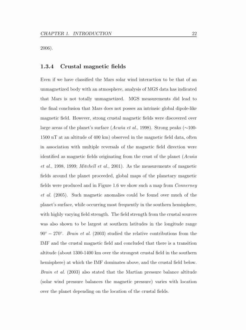
fields were produced and in Figure 1.6 we show such a map from Connerney
et al. (2005). Such magnetic anomalies could be found over much of the
planet’s surface, while occurring most frequently in the southern hemisphere,
with highly varying field strength. The field strength from the crustal sources
was also shown to be largest at southern latitudes in the longitude range
90◦ − 270◦. Brain et al. (2003) studied the relative contributions from the
IMF and the crustal magnetic field and concluded that there is a transition
altitude (about 1300-1400 km over the strongest crustal field in the southern
hemisphere) at which the IMF dominates above, and the crustal field below.
Brain et al. (2003) also stated that the Martian pressure balance altitude
(solar wind pressure balances the magnetic pressure) varies with location
over the planet depending on the location of the crustal fields.
CHAPTER 1. INTRODUCTION 23
Figure 1.6: A map of the global distribution of the crustal magnetic fieldsof Mars. The colour shows the median radial magnetic field at 400 kmfrom the filtered MGS measurements in each 1◦ × 1◦ latitude/longitudebin. Reproduced from Connerney et al. (2005).
Subsequently, global models of the crustal magnetic fields have been pro-
duced (Purucker et al., 2000; Cain et al., 2003; Arkani-Hamed , 2004; Langlais
et al., 2004). These models are all based on the MGS measurements but use
different methods. Cain et al. (2003) and Arkani-Hamed (2004) used spher-
ical harmonics up to the 90th order fitted to the data to describe the crustal
fields whereas Purucker et al. (2000) and Langlais et al. (2004) used binned
MGS data directly. The measured MGS data which are used in each model
(for either binning or for fitting to the spherical harmonic coefficients) are a
combination of IMF and crustal fields which introduces an error. The IMF
cannot be removed perfectly from the data. Secondly, the measurements
from MGS are performed at a certain altitude and consequently the crustal
field models are optimised for that altitude. Extrapolating to other altitudes

CHAPTER 1. INTRODUCTION 24
is not trivial and introduces further errors.
The crustal fields were subsequently shown to play a role in the structure
of the Martian plasma environment. Crider et al. (2002) used MGS data to
provide the first results that showed a latitude dependence of the altitude
of the MPB. The altitude of the MPB was shown to be higher for crossings
that occurred at high southern latitudes. In addition, within the longitude
range 90◦ − 270◦ where the crustal fields are strong, the distribution of the
terminator distances of the MPB was shown to be more scattered than for
crossings that occurred outside this longitude range (Crider et al., 2002).
Mazelle et al. (2004) used the same data set and discussed the possibility of
the crustal fields also affecting the BS but could not readily show it. The
effect of the crustal fields on the Martian plasma boundaries could be studied
further by using a larger data set from the MGS mission and by studying the
altitude of the BS as a function of the crustal field strength. This is a major
part of Chapter 3 and will also be touched upon in Chapters 4 and 5.
From MEX data, it was also determined that the altitude of the MPB
in terms of the altitude of magnetosheath electrons was dependent on the
crustal field strength (Franz et al., 2006b). In addition, Dubinin et al. (2008b)
detected a north-south asymmetry in the BS location. The BS in the south-
ern hemisphere was found to be located farther out than in the northern
hemisphere, independent of IMF direction. The asymmetry was assumed to
be caused by the crustal magnetic fields which pushed the boundary farther
out in the southern hemisphere.
Simulations of the solar wind interaction with Mars that include the
crustal sources do not appear to show any global changes in altitude of the
BS, but on a smaller scale it can make a difference, whereas the MPB seems
CHAPTER 1. INTRODUCTION 25
to be affected more, and especially over strong crustal sources where it forms
more of a magnetopause-like structure (Harnett and Winglee, 2007).
1.3.5 Global models of the Martian plasma environ-
ment
The global three-dimensional modelling of the Martian plasma environment
has been quite extensive in the past. This has helped in understanding the
solar wind interaction with Mars to a large extent. While spacecraft data
give invaluable information of the plasma system, simulations of the system
with global models help in testing theories of how the system is believed to
function. Spacecraft data can reveal small scale (spatial or temporal) features
while models tend to have much coarser spatial and temporal resolutions
due to computer limitations. But models have the advantage of giving a
view of the entire global picture at once, and it can also be used to study
the dependence of upstream solar wind conditions in a more straightforward
way, by changing the model’s boundary conditions.
There are essentially two types of models being used at present. MHD
models, which use the magnetohydrodynamic equations to describe the physics,
treating the plasma as a fluid (Ma et al., 2004; Terada et al., 2009). Hybrid
models, on the other hand, treating the electrons as a fluid while the ions
are treated as individual, kinetic particles (Modolo et al., 2006; Brecht and
Ledvina, 2006; Harnett and Winglee, 2007; Kallio et al., 2008; Boesswetter
et al., 2009).
No model can perfectly accurately reproduce the picture of the Martian
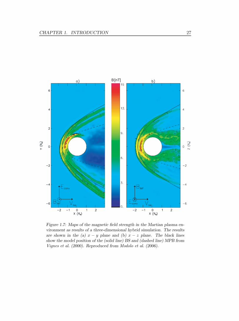
plasma environment that has risen from actual measurements. Figure 1.7
show an example of results from a simulation using the hybrid model of
CHAPTER 1. INTRODUCTION 26
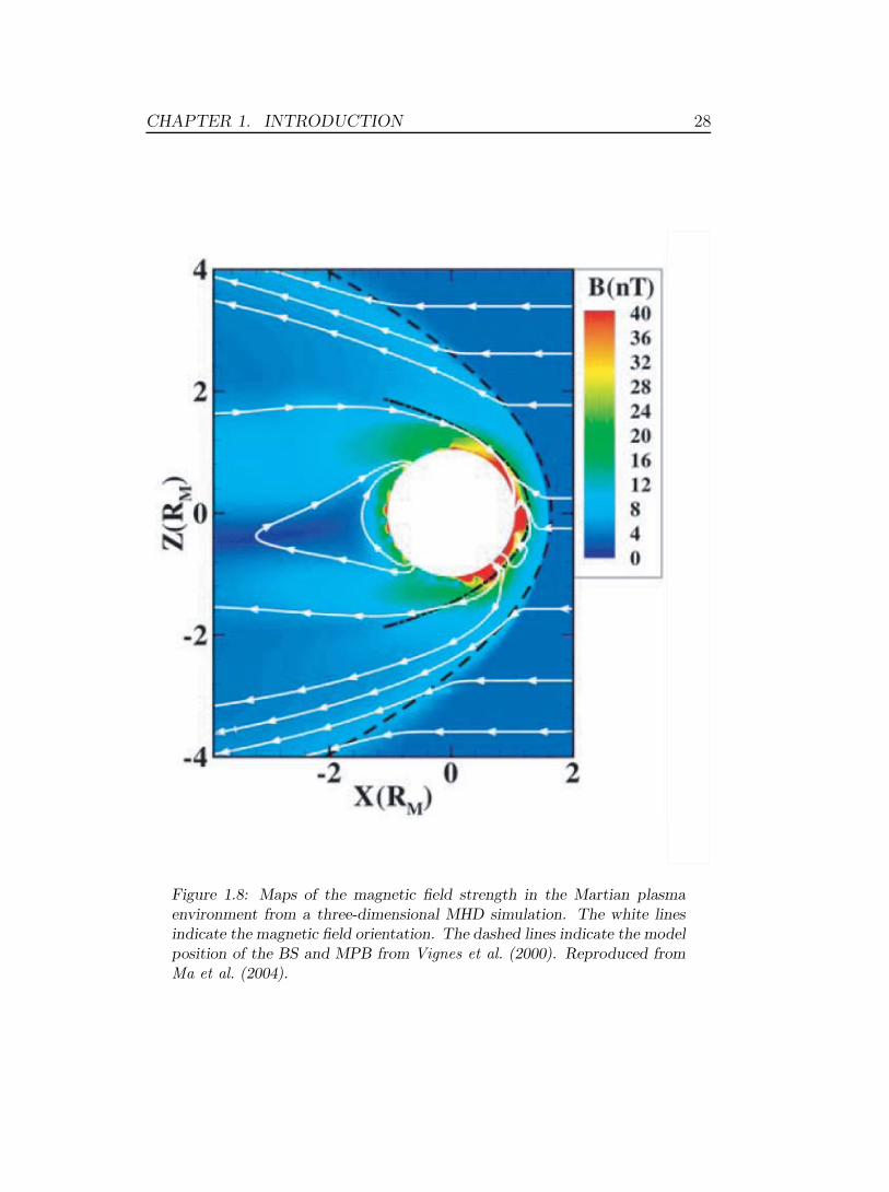
Modolo et al. (2006) and Figure 1.8 shows an example of the results from a
simulation using the MHD model of Ma et al. (2004). Both Figures show a
map of the magnetic field strength around Mars, with the Vignes et al. (2000)
models of the BS and the MPB superposed as black dashed and solid black
lines. In both models the MPB and the BS are reproduced at approximately
the same location as the empirical models suggest. The hybrid model takes
into account kinetic effects, due to the finite ion gyro radius, which includes
the asymmetry of the global environment caused by the convective electric
field. The magnetic field strength is much larger in the MHD model than in
the hybrid model in this case.
A recent study by Brain et al. (2009) shows the results of the first community-
wide comparison of all the above mentioned models when using the same
input conditions. The comparison shows a fairly large difference in terms of
where the plasma boundaries are located even though the input conditions
were the same. This reveals a weakness in the models in terms of their accu-
racy in describing the plasma system. The general picture was the same but
large differences in details were also reported.
1.3.6 Erosion of the atmosphere
Since Mars does not have a strong global magnetic field the atmosphere is
not shielded from the solar wind flow. This means that the ionosphere, con-
sisting mainly of CO+2 , O+ and O+
2 , could continuously be eroded and swept
away by the solar wind. This leads to an eventual erosion of the entire at-
mosphere. To what extent and through which exact processes this occurs
has been studied extensively. The first measurements of plasma escape came
from the Phobos 2 spacecraft where the oxygen ion escape rate was esti-
CHAPTER 1. INTRODUCTION 27
B [nT]
Figure 1.7: Maps of the magnetic field strength in the Martian plasma en-vironment as results of a three-dimensional hybrid simulation. The resultsare shown in the (a) x − y plane and (b) x − z plane. The black linesshow the model position of the (solid line) BS and (dashed line) MPB fromVignes et al. (2000). Reproduced from Modolo et al. (2006).
CHAPTER 1. INTRODUCTION 28
Figure 1.8: Maps of the magnetic field strength in the Martian plasmaenvironment from a three-dimensional MHD simulation. The white linesindicate the magnetic field orientation. The dashed lines indicate the modelposition of the BS and MPB from Vignes et al. (2000). Reproduced fromMa et al. (2004).
CHAPTER 1. INTRODUCTION 29
mated to be on the order of ∼3 · 1025 s−1, corresponding to a loss of the
present atmosphere in less than 100 million years (Lundin et al., 1989). The
physical process suggested for this escape to occur was ion pickup resulting
from the mass-loading of the solar wind in the plasma environment, as well
as ion beams from upward acceleration processes like those occurring in the
Earth’s auroral regions. Other possible processes that have been suggested
later are thermal (Jeans) escape, sputtering, ion outflow from crustal mag-
netic field cusps and bulk plasma removal (e.g. detached ionospheric clouds
caused by Kelvin-Helmholtz instabilities), see Carlsson et al. (2008) and ref-
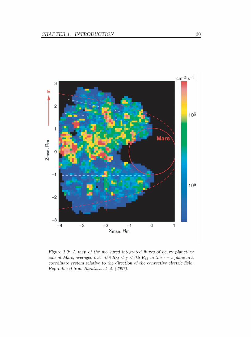
erences therein. Subsequently, more studies have been performed and after
the arrival of MEX the estimated escape rates have been adjusted downward
to be only on the order of ∼3 · 1023 s−1, significantly less than the first esti-
mated values (Barabash et al., 2007). Figure 1.9 shows a map from Barabash
et al. (2007) of these integrated fluxes at Mars from MEX measurements. It
was then suggested that water reservoirs, if there ever were any, could still
be present on Mars or alternatively, unknown escape channels could exist.
Solar forcing has been shown to increase the outflow as the observed ion es-
cape increases during periods of high dynamic pressure and high solar EUV
flux (Lundin et al., 2008) and the convective electric field has been shown to
govern in which hemisphere the outflow mainly takes place (Fedorov et al.,
2006). Sporadic outflow through ion beam events, when escaping planetary
ions are observed over a short time and in a narrow angle (beamed), also
predominantly occur in the hemisphere of locally upward convective electric
field (Carlsson et al., 2008). This can also be seen in Figure 1.9 where the
ion fluxes are higher in the hemisphere of the locally upward electric field.
Measurements of outflow at Mars have only been performed by MEX and
CHAPTER 1. INTRODUCTION 30
Figure 1.9: A map of the measured integrated fluxes of heavy planetaryions at Mars, averaged over -0.8 RM < y < 0.8 RM in the x− z plane in acoordinate system relative to the direction of the convective electric field.Reproduced from Barabash et al. (2007).
CHAPTER 1. INTRODUCTION 31
to some extent also by Phobos 2, but Phobos 2 did not have an adequate
coverage of measurements. MEX on the other hand does not carry a mag-
netometer which is important for determining the direction of the outflow.
It rather had to rely on magnetic field measurements from MGS during the
time of mission overlap. Also, far downstream and far off the Mars-Sun line,
measurements of the outflow have not been performed, which might be im-
portant for the total outflow rate. The measured outflow rates have been
compared with modelled values but since the latter span an order of mag-
nitude depending on which model is being used, this comparison does not
really provide much information (Brain et al., 2009). Measurements of the
outflow are needed from when simultaneous magnetic field data are present.
Also, estimates of the outflow rates during solar maximum are unknown and
need to be determined. Neither MEX nor Phobos 2 sampled the Martian
plasma environment during solar maximum. The cold ion population is not
detectable by the ion mass analyzer instrument on MEX which could mean
that a significant portion of the potentially escaping cold plasma is being
missed.

Chapter 2Instrumentation
In this Thesis we have used data from eight instruments onboard three space-
craft. These instruments will be described in this Chapter together with their
host spacecraft and the spacecraft’s orbital geometry.
2.1 Mars Global Surveyor: magnetometer and
electron reflectometer
MGS arrived at Mars in September 1997 and stayed operational in orbit for
9 years, until November 2006. During the initial (pre-mapping) phase of the
mission, which lasted from September 1997 until January 1999, MGS used
an aerobreaking technique to slowly alter the spacecraft orbit. The orbit
evolved from highly elliptical and precessing in local time to become almost
circular, polar and fixed at 02h-14h local time when the 7.5 year long mapping
phase began. Periapsis during the pre-mapping phase was at a minimum of
∼100 km and apoapsis at a maximum of ∼17 RM (1 RM = 3397 km) and
the nearly constant altitude during the mapping phase was ∼400 km. The
32
CHAPTER 2. INSTRUMENTATION 33
orbital coverage during the pre-mapping phase and mapping phase is shown
in Figure 2.1 in MSO coordinates.
Relevant for plasma studies, MGS carried a magnetic field investigation
(MAG) (Acuna et al., 1998) and an electron reflectometer (ER) (Mitchell
et al., 2001). The MAG instrument consisted of two fluxgate magnetometers
mounted on the tips of the solar panels, about 5 m from the main spacecraft
bus. It provided vector measurements of the magnetic field at a rate of 2 Hz –
16 Hz, depending on telemetry rate, in the range ±4 nT – ±65, 536 nT (Acuna
et al., 1998). The ER instrument measured the local electron distribution
function in 30 energy levels in the range∼1 eV – 20 keV with a maximum time
resolution of 0.5 Hz and energy resolution of 25% . The instrument had a field
of view of 360◦ × 14◦ divided on 16 sectors (Mitchell et al., 2001). Plasma
moments (density, velocity and temperature) can usually not be reliably
calculated from the electron distribution measured by ER due to the poor
energy resolution.
2.2 Mars Express: ASPERA-3 and MARSIS
MEX arrived at Mars in late 2003 and is still operational in orbit (as of 2009).
It had almost three years of overlapping data coverage with MGS, until MGS
died in late 2006. The orbit of MEX is highly elliptical and precessing in local
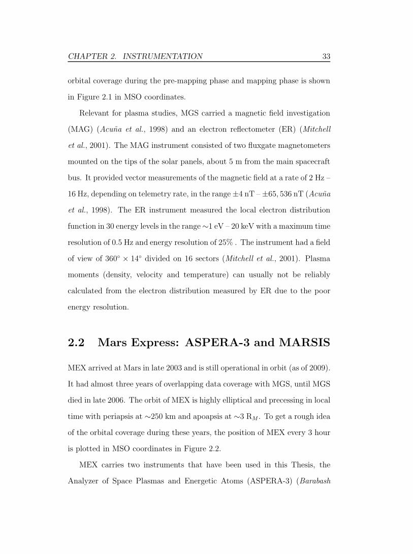
time with periapsis at ∼250 km and apoapsis at ∼3 RM . To get a rough idea
of the orbital coverage during these years, the position of MEX every 3 hour
is plotted in MSO coordinates in Figure 2.2.
MEX carries two instruments that have been used in this Thesis, the
Analyzer of Space Plasmas and Energetic Atoms (ASPERA-3) (Barabash

CHAPTER 2. INSTRUMENTATION 34
a
fe
dc
b
Figure 2.1: The position of MGS every 1 hour in MSO coordinates duringthe pre-mapping phase from September 1997 until January 1999 plottedin (a) cylindrical coordinates as well as in Cartesian coordinates projectedonto the (b) x−y, (c) x−z and (d) y−z plane. The position every 4 hoursduring the mapping phase is plotted in (e) cylindrical coordinates and (f)projected onto the y − z plane. The average BS (red line) and MPB (blueline) position from Trotignon et al. (2006) are shown in panels (a) and (e).
CHAPTER 2. INSTRUMENTATION 35
a b
dc
Figure 2.2: The position of MEX every 3 hours in MSO coordinates from2004 until 2008. The position is shown in (a) cylindrical coordinates to-gether with the average position of the BS (red line) and MPB (blue line)from Trotignon et al. (2006) and in Cartesian coordinates projected ontothe (b) x − y, (c) x − z and (d) y − z planes.
CHAPTER 2. INSTRUMENTATION 36
et al., 2006) and the Mars Advanced Radar for Subsurface and Ionospheric
Sounding (MARSIS) (Gurnett et al., 2005). Related to space physics, MEX
also performs radio occultation measurements of the ionosphere through the
MaRS experiment and measures UV spectra with the SPICAM instrument,
but data from these have not been included in this Thesis. ASPERA-3
includes four sensors out of which two have been used in this Thesis, the
electron spectrometer (ELS) and the ion mass analyzer (IMA). ELS is similar
to ER on MGS and measures the electron distribution in the energy range 10
eV – 20 keV, but with a higher energy resolution (8%) and a time resolution of
0.25 Hz. The field of view is 4◦×360◦ divided into 16 sectors. IMA measures
the local ion distribution function in the energy range 10 eV/q – 36 keV/q
for the main ion species, H+, H+2 , He+ and O+ and for the molecular group of
ions in the mass per charge range 20 < amu/q < 80. It has a time resolution
of 192 s and a field of view of 90◦ × 360◦. Density, velocity and temperature
moments can be calculated from both IMA and ELS, as descried by Franz
et al. (2006a).
MARSIS is a 40 m long dipolar antenna designed for subsurface as well as
ionospheric sounding. However, it can occasionally also measure local plasma
density and magnetic field magnitude, respectively, from observed harmonics
of the electron plasma oscillations and electron cyclotron echoes seen in the
radargrams (Gurnett et al., 2005; Duru et al., 2008). Since MEX does not
carry a magnetometer and since ASPERA-3 cannot measure the cold plasma
population very well, these extra properties of the sounder have become very
valuable.
CHAPTER 2. INSTRUMENTATION 37
2.3 Rosetta: The Rosetta Plasma Consortium
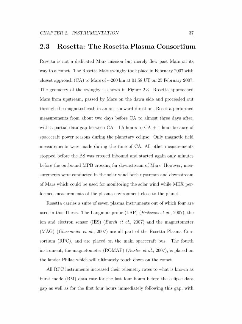
Rosetta is not a dedicated Mars mission but merely flew past Mars on its
way to a comet. The Rosetta Mars swingby took place in February 2007 with
closest approach (CA) to Mars of ∼260 km at 01:58 UT on 25 February 2007.
The geometry of the swingby is shown in Figure 2.3. Rosetta approached
Mars from upstream, passed by Mars on the dawn side and proceeded out
through the magnetosheath in an antisunward direction. Rosetta performed
measurements from about two days before CA to almost three days after,
with a partial data gap between CA - 1.5 hours to CA + 1 hour because of
spacecraft power reasons during the planetary eclipse. Only magnetic field
measurements were made during the time of CA. All other measurements
stopped before the BS was crossed inbound and started again only minutes
before the outbound MPB crossing far downstream of Mars. However, mea-
surements were conducted in the solar wind both upstream and downstream
of Mars which could be used for monitoring the solar wind while MEX per-
formed measurements of the plasma environment close to the planet.
Rosetta carries a suite of seven plasma instruments out of which four are
used in this Thesis. The Langmuir probe (LAP) (Eriksson et al., 2007), the
ion and electron sensor (IES) (Burch et al., 2007) and the magnetometer
(MAG) (Glassmeier et al., 2007) are all part of the Rosetta Plasma Con-
sortium (RPC), and are placed on the main spacecraft bus. The fourth
instrument, the magnetometer (ROMAP) (Auster et al., 2007), is placed on
the lander Philae which will ultimately touch down on the comet.
All RPC instruments increased their telemetry rates to what is known as
burst mode (BM) data rate for the last four hours before the eclipse data
gap as well as for the first four hours immediately following this gap, with
CHAPTER 2. INSTRUMENTATION 38
-30
-20
-10
0
10
20
30
-10
0
10-202
X [RM
] Y [RM
]
Z [R
M]
Rosetta pathRosetta data gapRosetta startMars Express path
Figure 2.3: The trajectory of Rosetta and MEX from 22:38 UT on February24, 2007, until 05:28 UT on February 25, 2007, plotted as blue and red linesin MSO coordinates. The projections of the trajectories and the planet onthe x−y, x−z and y−z planes are shown as black lines. Rosetta approachesMars from the dayside and proceeds out along the magnetic tail. The startis indicated by a blue star. The gap in the Rosetta RPC data is shown asa cyan line.
normal mode (NM) sampling at a lower rate outside this interval. The LAP
instrument operated in bias current mode during the swingby, measuring the
probe-to-spacecraft potential Vps at 57.8 Hz in BM and 0.9 Hz in NM. LAP
consists of two probes, of which only probe 1, mounted on the slightly longer
boom, has been used in this Thesis, as probe 2 was mostly in eclipse and
could therefore not be used for Vps measurements. MAG sampled the three-
axis magnetic field at 20 Hz in BM and 1 Hz in NM. RPC-MAG data are
more reliable than ROMAP data when other instruments are in operation
since the MAG sensor is placed on a boom and thus farther away from the
spacecraft body. During CA all other instruments were switched off and
the ROMAP data were not disturbed. Magnetic field data from ROMAP
thus exist for the entire Mars flyby, at a sampling rate of 32 Hz around
CHAPTER 2. INSTRUMENTATION 39
CA and then at a sampling rate of 1 Hz a few hours before and after the
CA interval time. IES recorded electron and ion energy spectra with a time
resolution of 128 s in BM. The combined (ion and electron) IES telemetry
rate is 253 bps in BM and 50 bps in NM. Due to field of view limitations
(2π steradians around the instrument equator) combined with having the
instrument behind the spacecraft as seen from the Sun, the full solar wind
ion flow was not accessible to IES, meaning that a useful plasma density
estimate cannot be readily produced from the IES ion data. However, the
energy information in IES data can be directly interpreted, and can be used
to show the presence and speed of the solar wind even though only a part of
the flow can be detected.
2.4 Moments from ion and electron measure-
ments
The spectra measured by electron and ion instruments give useful information
about the plasma but of further interest are the values of the density, velocity
and temperature of the plasma. These quantities can be derived from the
spectrograms and in this Section we will briefly describe how.
The particle instruments used in this Thesis measure single electrons and
ions at a certain energy E (and sometimes masses for the ions), over a certain
solid angle Ω, at a certain position r and at a time t, which is a quantity
called differential flux J(E, Ω, r, t). The relation between the differential flux
and the local phase-space distribution function f(r,v, t) is
J(E, Ω, r, t) =v2
mf(r,v, t), (2.1)

CHAPTER 2. INSTRUMENTATION 40
where m is the mass and v is the velocity. The density n, bulk velocity vector
V and pressure tensor P moments can be calculated from the distribution
function as
n(r, t) =
∫v
f(r,v, t)d3v, (2.2)
n(r, t)V(r, t) =
∫v
vf(r,v, t)d3v, (2.3)
and
P(r, t) =
∫v
mvvf(r,v, t)d3v. (2.4)
The temperature can then be calculated as T = P/nk, where k is Boltz-
mann’s constant.
Another way of obtaining the plasma moments is to assume that the
phase-space density of the particles has a Maxwellian distribution in velocity
space. Then the density and thermal energy can in principle be obtained
by fitting a Maxwellian curve to the measured spectra. A more thorough
description of how the moments are calculated from the ELS and IMA can be
found in Franz et al. (2006a). The spacecraft potential, which mostly affects
low-energy electrons, and the geometric factor (sensitivity of the detector
surface multiplied by solid angle) also needs to be taken into account to
produce accurate moments.
CHAPTER 2. INSTRUMENTATION 41
2.5 Rosetta and Mars Express density cross-
calibration
The Rosetta LAP instrument measured probe-to-spacecraft potential Vps
during the Mars flyby. This is assumed to be related to plasma density
which is of further interest in Chapter 4 of this Thesis, and we have un-
dertaken a first basic calibration of the Langmuir probe density estimates
using density measurements from MEX ELS. The material presented in this
Section is published in Edberg et al. (2009c).
To calibrate the measurements of Vps by Rosetta LAP to MEX ELS
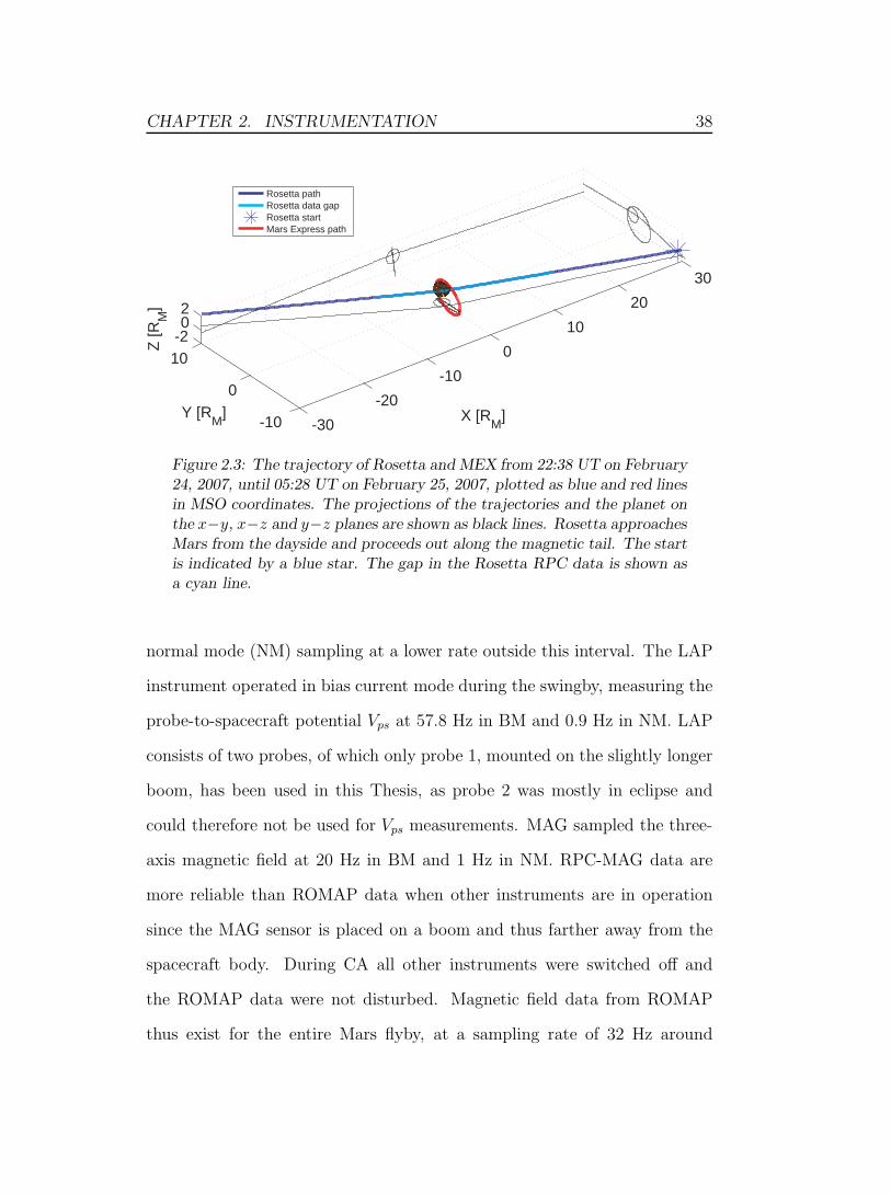
plasma density moments, we need reliable comparison data. Figure 2.4 shows
MEX ELS electron density moment and Rosetta LAP Vps data in the solar
wind for the days following the Rosetta flyby. During this period, Rosetta
was in the solar wind downstream of Mars and MEX, so that similar solar
wind conditions can be reasonably assumed, at least on a statistical basis. To
produce directly comparable datasets, the ELS data have been time shifted
to the time line of Rosetta by adding a solar wind propagation time based on
the difference in the MSO x-coordinate between the two spacecraft and the
solar wind velocity derived from the energy at the peak in the IMA spectra.
For most of this period, the attitude of Rosetta was stable, except for one
change of about 40◦ of the solar aspect angle (SAA), i.e. the angle between
the spacecraft z-axis and the direction to the Sun. This corresponds to a
rotation about the y-axis which is parallel to the solar panels. The SAA was
however never more than 50◦ from its value during the period of main sci-
entific interest, i.e. around the time of CA, which is necessary for a reliable
calibration. For this reason, we do not include data from the days preceding
CHAPTER 2. INSTRUMENTATION 42
0
2
4
6
8
Ne (
ME
X)
cm-3
-1.5
-1
-0.5
0
0.5
Vps
[V]
12:00 15:00 18:00 21:00 00:00 03:00 06:00 09:00 12:00 15:00 18:00
-80
-60
-40
-20
0
UT on 25 26 February 2007 (HH:MM)
SA
A[0 ]
Excluded Excluded
Exc
lude
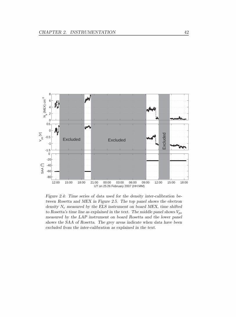
d
Figure 2.4: Time series of data used for the density inter-calibration be-tween Rosetta and MEX in Figure 2.5. The top panel shows the electrondensity Ne measured by the ELS instrument on board MEX, time shiftedto Rosetta’s time line as explained in the text. The middle panel shows Vps
measured by the LAP instrument on board Rosetta and the lower panelshows the SAA of Rosetta. The grey areas indicate when data have beenexcluded from the inter-calibration as explained in the text.
CHAPTER 2. INSTRUMENTATION 43
the Rosetta flyby in the calibration since the SAA was very different then.
The solar wind does not show any significant variability during the days be-
fore the flyby either, which is necessary for this type of calibration. Small
structures in the solar wind are not easily observed at two very distant (up
to 300 RM in this case) positions in space and would only bias the calibration
by adding a lot of data points around one specific value. We point out that
this will be an approximate calibration but still reasonably good.
Periods during which the Rosetta attitude is changing rapidly, and where
there are data gaps in the MEX data or when MEX is not in the solar wind,
have also been excluded from the data sets, and are shaded in Figure 2.4.
While some details differ, as expected in the dynamic solar wind, it is clear
that the main features in the two data sets are the same, including a signif-
icant decrease in plasma density before noon on February 26 as well as the
general trends in the data.
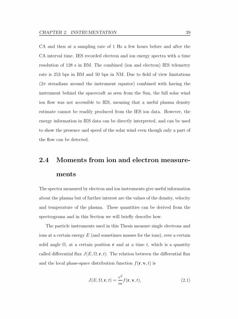
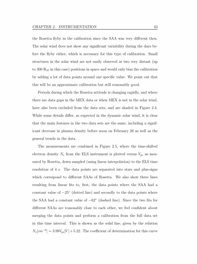
The measurements are combined in Figure 2.5, where the time-shifted
electron density Ne from the ELS instrument is plotted versus Vps as mea-
sured by Rosetta, down sampled (using linear interpolation) to the ELS time
resolution of 4 s. The data points are separated into stars and plus-signs
which correspond to different SAAs of Rosetta. We also show three lines
resulting from linear fits to, first, the data points where the SAA had a
constant value of −25◦ (dotted line) and secondly to the data points where
the SAA had a constant value of −62◦ (dashed line). Since the two fits for
different SAAs are reasonably close to each other, we feel confident about
merging the data points and perform a calibration from the full data set
in this time interval. This is shown as the solid line, given by the relation
Ne[cm−3] = 3.98Vps[V ]+5.22. The coefficient of determination for this curve
CHAPTER 2. INSTRUMENTATION 44
-1. 5 -1 -0. 5 0 0.50
1
2
3
4
5
6
7
8
Vps
(ROS) [V]
Ne
(ME
X)
[cm
]
-3
Figure 2.5: The electron density Ne measured by the ELS instrument onMEX plotted versus probe-to-spacecraft potential Vps measured by theLAP instrument on Rosetta. Stars and plus-signs denote different SAAs ofRosetta (−25◦ and −62◦, respectively). The data were taken from intervalsas described in Figure 2.4. The solid line is a fitted curve to all of the datawhereas the dotted and dashed lines are a fits to the data obtained whenthe SAA of Rosetta was −25◦ and −62◦, respectively. The linear relationof the solid curve between Vps and Ne (Ne[cm−3] = 3.98Vps[V ] + 5.22) isused to estimate the density from LAP Vps measurements.

CHAPTER 2. INSTRUMENTATION 45
is 0.95.
While the linear fit to the data points is quite good, with an inevitable
spread caused by the dynamic and inhomogeneous nature of the solar wind,
the spacecraft potential is usually expected to be a logarithmic function of the
plasma density, as the photoelectrons emitted are usually assumed to have an
exponential distribution with energy. This is indeed close to what is observed
on Earth-orbiting satellites equipped with long wire booms extending far
from the perturbations caused by the spacecraft body (Thiebault et al., 2006;
Pedersen et al., 2008). However, for the short booms of Rosetta (2.24 m and
1.62 m), we can expect to see only a fraction of the spacecraft potential.
To this fraction should be added important contributions from the potential
fields generated by the solar panels and also the potential drop over the probe
sheath: the latter is on the order of a volt, which clearly is of the same order
as the measured Vps. Hence, we cannot expect to find a logarithmic relation,
valid for a large range of potentials. The observed good linear correlation in
Figure 2.5 should therefore not be extrapolated far outside the given interval,
and should be interpreted rather as a linear expansion of a full Ne-Vps relation
in the interval shown. As the details of this relation also depend on, for
example, the UV intensity (Pedersen et al., 2008; Eriksson and Winkler ,
2008), the validity outside the flyby interval is further reduced. Nevertheless,
the statistical correlation seen in Figure 2.5 as well as the obvious co-variation
in Figure 2.4 shows that the linear calibration can be used for the data we
are interested in, accurate to a factor of about 2 for Vps in the range -0.7 V
to +0.5 V, assuming that the density from MEX is correct. We do not say
that this is the final calibration that will be used when Rosetta reaches the
comet but simply that it gives a rough estimate of the density for now.

Chapter 3Mars Global Surveyor measurements
of the influence of the crustal magnetic
fields
In this Chapter we examine the shape and location of the BS and MPB using
the data set from the MGS spacecraft. We also study the influence of the
crustal magnetic fields on these two boundaries as well as study the magnetic
field strength inside the MPB. Some of the material presented in this chapter
is published in Edberg et al. (2008).
3.1 Introduction
Mars has been considered to be a mainly unmagnetized body in the past
and the solar wind interaction with Mars have therefore been expected to be
very similar to that of Venus and comets. However, the discovery of strong
crustal magnetic fields on localized places on Mars, by the MGS spacecraft,
have somewhat changed this view. As MGS orbited Mars during the first 1.5
46
CHAPTER 3. MARS GLOBAL SURVEYOR MEASUREMENTS OFTHE INFLUENCE OF THE CRUSTAL MAGNETIC FIELDS 47
years after arrival in late 1997 it repeatedly crossed the BS and the MPB in
the Martian plasma environment. This large data set of crossings can be used
to produce statistical best-fit models of the boundaries as well as to study the
variation of the boundaries with the crustal magnetic fields. The boundary
shapes have already been studied in the past but with smaller subsets of the
data and the influence of the crustal magnetic fields have only been touched
upon briefly. In this Chapter we will complement the previous studies by
using the full data set and study the influence of the crustal magnetic fields
in more detail. We start off by introducing one example of boundary crossings
in the MGS MAG/ER data set. We then use all similarly observed boundary
crossings in order to model the shape of the boundaries and to determine the
influence of the crustal magnetic fields.
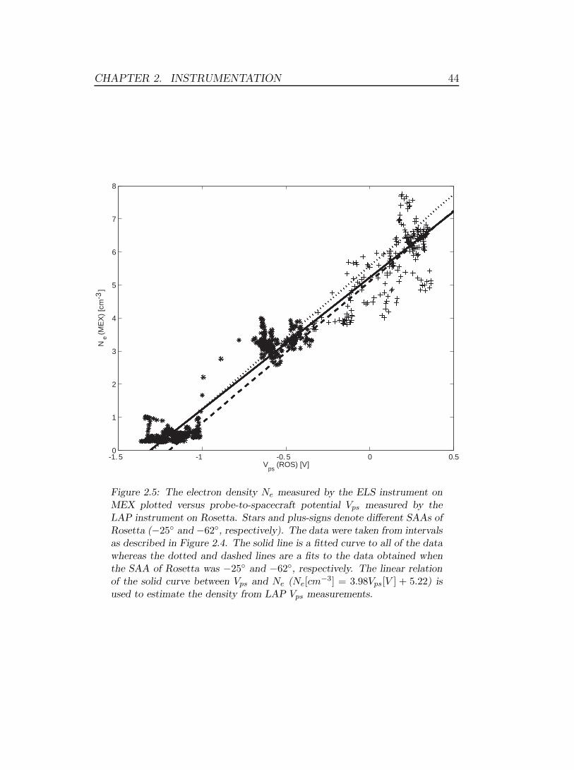
3.2 Data analysis
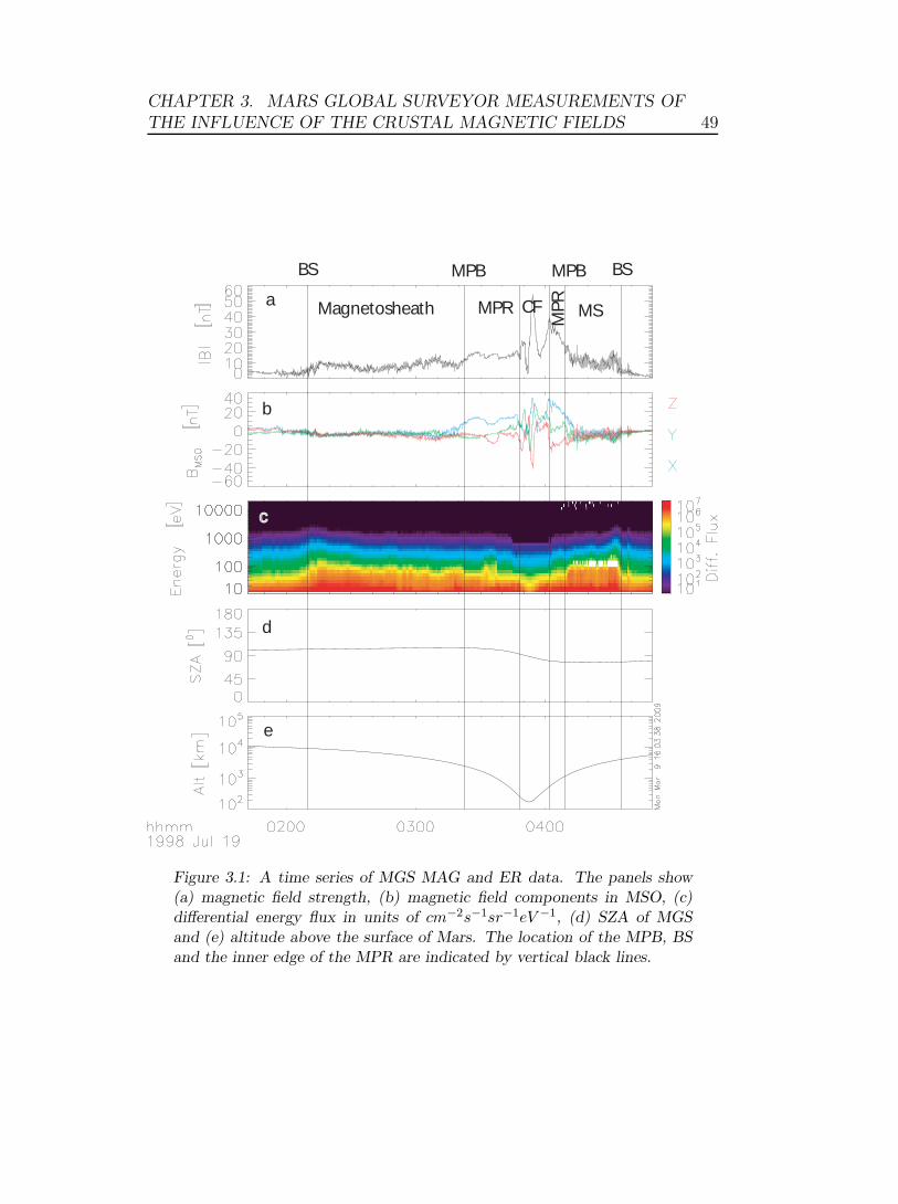
Figure 3.1 shows an example of a time series from MGS. The orbit at this time
was highly elliptical, nearly polar and close to the terminator plane. The top
two panels show the magnetic field measurements from the MAG instrument.
The following panel shows differential energy flux from the ER instrument.
The bottom two panels show SZA of the spacecraft and altitude above the
surface of Mars. The inbound BS crossing is identified in the MAG/ER data
as an increase in magnetic field fluctuations together with an increase in
electron fluxes at around 02:10 UT. The spacecraft then entered the magne-
tosheath, characterized by heated plasma and more turbulent magnetic field.
The crossing of the MPB is identified by three simultaneous features in the
data at 03:22 UT. The most obvious signature is a fairly sudden increase in
CHAPTER 3. MARS GLOBAL SURVEYOR MEASUREMENTS OFTHE INFLUENCE OF THE CRUSTAL MAGNETIC FIELDS 48
the magnitude of the magnetic field. In addition, the strong fluctuations in
the magnetic field which occur in the magnetosheath inside the BS stop at
this boundary and thirdly, the electron flux decreases compared to values in
the magnetosheath. A fourth signature can sometimes also be seen, which is
the beginning of the draping (rotation of the field direction) of the field lines
around the planet. After the inbound MPB crossing MGS is inside the MPR
until 03:48 UT followed by a period close to crustal magnetic field sources.
The MPR is entered again at 04:02 UT, the outbound MPB crossing occurs
at around 04:09 UT and the outbound BS crossing at 04:35 UT. We have
examined the entire MAG and ER data set from the pre-mapping phase of
the mission in search of such crossings of the MPB and BS. We found a total
of 993 and 619 crossings, respectively. The reason for the fewer BS crossings
is that the MAG and ER instruments only operated around CA after the
first 12 months, such that the MPB could be observed, but not the BS which
was too far out. The number of crossings found in this study differs from
that by Trotignon et al. (2006) (573 BS crossings and 860 MPB crossings)
and Bertucci et al. (2005) (1149 MPB crossings), who also used the entire
data set. This is explained by the fact that the boundaries can be difficult to
determine in some cases, e.g. when the orbit is tangential to the boundary
surface or when the crossings occur close to strong crustal anomalies. Some
crossings might be included in some studies and ruled out as too uncertain
in others. Unusual solar wind conditions can also disturb the appearance of
the boundaries, thus making them hard to identify.
CHAPTER 3. MARS GLOBAL SURVEYOR MEASUREMENTS OFTHE INFLUENCE OF THE CRUSTAL MAGNETIC FIELDS 49
BS BSMPB MPB
Magnetosheath MPR
MPRCF MS
a
b
c
d
e
Figure 3.1: A time series of MGS MAG and ER data. The panels show(a) magnetic field strength, (b) magnetic field components in MSO, (c)differential energy flux in units of cm−2s−1sr−1eV −1, (d) SZA of MGSand (e) altitude above the surface of Mars. The location of the MPB, BSand the inner edge of the MPR are indicated by vertical black lines.
CHAPTER 3. MARS GLOBAL SURVEYOR MEASUREMENTS OFTHE INFLUENCE OF THE CRUSTAL MAGNETIC FIELDS 50
Table 3.1: Best fit conic section parameters of the MPB obtained in thisstudy, with and without a fixed subsolar standoff distance, as well as forthe studies by Vignes et al. (2000) and Trotignon et al. (2006). The un-certainties are calculated differently here (see text for explanation), whichexplains the large difference in uncertainty values compared with the stud-ies by Vignes et al. (2000) and Trotignon et al. (2006). N is the number ofdata points. See Section 1.3.2 for explanations of X0, ε and L.
Study by X0 ε L RSS N[RM ] [RM ] [RM ]
This study 0.86±0.11 0.92±0.03 0.90±0.06 1.33±0.15 993This study, fixed RSS 0.73±0.11 0.90±0.03 0.98±0.06 1.25 993Vignes et al. (2000) 0.78±0.01 0.90±0.01 0.96±0.01 1.29±0.04 488Trotignon et al. (2006) (x > 0) 0.64±0.01 0.77±0.01 1.08±0.03 1.25±0.03 901Trotignon et al. (2006) (x < 0) 1.60 1.009±0.003 0.528±0.012 901
3.2.1 Shape of bow shock and magnetic pileup bound-
ary
In the upper two panels of Figure 3.2 all observed crossings of the BS and
MPB are plotted in a cylindrical coordinate system. The horizontal axis is the
aberrated MSO x-axis, while the vertical axis is the perpendicular distance
from the x-axis =√
y2 + z2. The variability of the crossing position is large,
and larger on the night side than on the day side. In order to determine
the best fit shape of the BS and MPB we use in principal the same method
as Vignes et al. (2000) and fit a conic section to the data points, with the
difference that we use the entire data set and not just the first year of data
as used in Vignes et al. (2000). This is done for both the MPB and for
the BS. In the lower panels (c and d) of Figure 3.2 are shown the best fit
conic sections determined here (solid line) together with the fits obtained by
Vignes et al. (2000) (dashed line) and Trotignon et al. (2006) (dashed-dotted
line). The dotted line in panel (d) shows a constrained fit to be described in
more detail later in this subsection. The parameters of the fits are shown in
Table 3.1 for the MPB and in Table 3.2 for the BS.
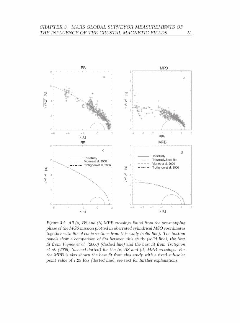
CHAPTER 3. MARS GLOBAL SURVEYOR MEASUREMENTS OFTHE INFLUENCE OF THE CRUSTAL MAGNETIC FIELDS 51
Y +
Z
22
[R ] M
Y +
Z
22
[R ] M
X [R ]M
X [R ]M
This studyVignes et al., 2000Trotignon et al., 2006
Y +
Z
22
[R ] M
X [R ]M
X [R ]M
Y +
Z
22
[R ] M
This study, fixed RssThis study
Vignes et al., 2000Trotignon et al., 2006
a b
cd
BS
BS
MPB
MPB
Figure 3.2: All (a) BS and (b) MPB crossings found from the pre-mappingphase of the MGS mission plotted in aberrated cylindrical MSO coordinatestogether with fits of conic sections from this study (solid line). The bottompanels show a comparison of fits between this study (solid line), the bestfit from Vignes et al. (2000) (dashed line) and the best fit from Trotignonet al. (2006) (dashed-dotted) for the (c) BS and (d) MPB crossings. Forthe MPB is also shown the best fit from this study with a fixed sub-solarpoint value of 1.25 RM (dotted line), see text for further explanations.

CHAPTER 3. MARS GLOBAL SURVEYOR MEASUREMENTS OFTHE INFLUENCE OF THE CRUSTAL MAGNETIC FIELDS 52
Table 3.2: Best fit conic section parameters for the BS obtained in thisstudy, as well as in the studies by Vignes et al. (2000) and Trotignon et al.(2006). N is the number of BS crossings.
Study by X0 ε L RSS N[RM ] [RM ] [RM ]
This study 0.55±0.12 1.05±0.04 2.10±0.09 1.58±0.18 619Vignes et al. (2000) 0.64±0.02 1.03±0.01 2.04±0.02 1.64±0.08 450Trotignon et al. (2006) 0.6 1.026±0.002 2.081±0.006 1.63±0.01 700
A difference that is introduced here compared to Vignes et al. (2000) is
that we define the outer surface of the MPB and BS to be the actual position
of the boundary crossing. This makes it necessary to calculate the uncertainty
of the fit in a different way. Vignes et al. (2000) repeated the fitting method
a great number of times, and because different random locations within the
boundary were used for the position of each crossing each time, an uncertainty
could be estimated. In this study, we calculate the uncertainty by varying
the fit parameters individually from the best fit value, until the root mean
square deviation of the data points changed by 5%. The uncertainty is then
chosen as the difference between the best fit parameter value and the value
that makes the RMS deviation change by 5%. The uncertainty estimates
obtained in this way are larger than those obtained by Vignes et al. (2000),
but since they are calculated differently they cannot be easily compared with
each other.
From Figure 3.2, panel (d), it can be seen that the best fit to the MPB
data from this study agrees well with the previous study by Vignes et al.
(2000), who only used a subset of the data. However, there are some differ-
ences. The subsolar standoff distance, calculated as
RSS = X0 +L
1 + ε, (3.1)
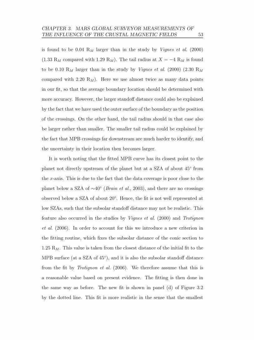
CHAPTER 3. MARS GLOBAL SURVEYOR MEASUREMENTS OFTHE INFLUENCE OF THE CRUSTAL MAGNETIC FIELDS 53
is found to be 0.04 RM larger than in the study by Vignes et al. (2000)
(1.33 RM compared with 1.29 RM). The tail radius at X = −4 RM is found
to be 0.10 RM larger than in the study by Vignes et al. (2000) (2.30 RM
compared with 2.20 RM). Here we use almost twice as many data points
in our fit, so that the average boundary location should be determined with
more accuracy. However, the larger standoff distance could also be explained
by the fact that we have used the outer surface of the boundary as the position
of the crossings. On the other hand, the tail radius should in that case also
be larger rather than smaller. The smaller tail radius could be explained by
the fact that MPB crossings far downstream are much harder to identify, and
the uncertainty in their location then becomes larger.
It is worth noting that the fitted MPB curve has its closest point to the
planet not directly upstream of the planet but at a SZA of about 45◦ from
the x-axis. This is due to the fact that the data coverage is poor close to the
planet below a SZA of ∼40◦ (Brain et al., 2003), and there are no crossings
observed below a SZA of about 20◦. Hence, the fit is not well represented at
low SZAs, such that the subsolar standoff distance may not be realistic. This
feature also occurred in the studies by Vignes et al. (2000) and Trotignon
et al. (2006). In order to account for this we introduce a new criterion in
the fitting routine, which fixes the subsolar distance of the conic section to
1.25 RM . This value is taken from the closest distance of the initial fit to the
MPB surface (at a SZA of 45◦), and it is also the subsolar standoff distance
from the fit by Trotignon et al. (2006). We therefore assume that this is
a reasonable value based on present evidence. The fitting is then done in
the same way as before. The new fit is shown in panel (d) of Figure 3.2
by the dotted line. This fit is more realistic in the sense that the smallest
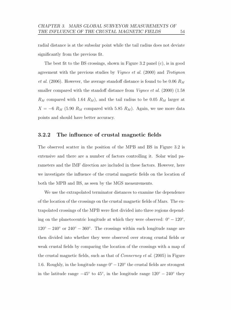
CHAPTER 3. MARS GLOBAL SURVEYOR MEASUREMENTS OFTHE INFLUENCE OF THE CRUSTAL MAGNETIC FIELDS 54
radial distance is at the subsolar point while the tail radius does not deviate
significantly from the previous fit.
The best fit to the BS crossings, shown in Figure 3.2 panel (c), is in good
agreement with the previous studies by Vignes et al. (2000) and Trotignon
et al. (2006). However, the average standoff distance is found to be 0.06 RM
smaller compared with the standoff distance from Vignes et al. (2000) (1.58
RM compared with 1.64 RM), and the tail radius to be 0.05 RM larger at
X = −6 RM (5.90 RM compared with 5.85 RM). Again, we use more data
points and should have better accuracy.
3.2.2 The influence of crustal magnetic fields
The observed scatter in the position of the MPB and BS in Figure 3.2 is
extensive and there are a number of factors controlling it. Solar wind pa-
rameters and the IMF direction are included in these factors. However, here
we investigate the influence of the crustal magnetic fields on the location of
both the MPB and BS, as seen by the MGS measurements.
We use the extrapolated terminator distances to examine the dependence
of the location of the crossings on the crustal magnetic fields of Mars. The ex-
trapolated crossings of the MPB were first divided into three regions depend-
ing on the planetocentric longitude at which they were observed: 0◦ − 120◦,
120◦ − 240◦ or 240◦ − 360◦. The crossings within each longitude range are
then divided into whether they were observed over strong crustal fields or
weak crustal fields by comparing the location of the crossings with a map of
the crustal magnetic fields, such as that of Connerney et al. (2005) in Figure
1.6. Roughly, in the longitude range 0◦−120◦ the crustal fields are strongest
in the latitude range −45◦ to 45◦, in the longitude range 120◦ − 240◦ they

CHAPTER 3. MARS GLOBAL SURVEYOR MEASUREMENTS OFTHE INFLUENCE OF THE CRUSTAL MAGNETIC FIELDS 55
Table 3.3: Average extrapolated MPB terminator distances and standarddeviations in units of RM divided into three longitude ranges and subdi-vided into whether they are observed over weak or strong crustal fields, asdescribed in the text.
Longitude range0◦ − 120◦ 120◦ − 240◦ 240◦ − 360◦
Strong crustal fields 1.48±0.18 1.55±0.24 1.48±0.18Weak crustal fields 1.38±0.12 1.43±0.15 1.41±0.12
are strongest in the latitude range −90◦ to 0◦ and in the longitude range
240◦ − 360◦ they are again strongest in the latitude range −45◦ to 45◦.
In Figure 3.3 the extrapolated terminator distance is plotted as a function
of Martian longitude. The mean terminator distance is shown in each of the
three longitude sections for crossings that occurred over strong crustal fields
(solid lines) and for crossings that were observed over weak crustal fields
(dashed lines), based on the latitude and longitude limits given above. The
figure shows that the MPB is on average located farther out when there are
strong crustal sources underneath. The scatter of the terminator distances
is again extensive. However, the differences in the averages for crossings
observed above strong and weak crustal fields are statistically significant
in each of the three longitude sections, according to a Student’s t-test at
a 95% confidence level. The average altitudes and corresponding standard
deviations for the MPB crossings are shown in Table 3.3. Our results are
in agreement with the results obtained by Crider et al. (2002) who showed
that the MPB was located farther out for high southern latitudes. The study
reported here shows that it is not only in the southern hemisphere where the
MPB altitude is raised by the crustal sources, but rather that the boundary
is affected more locally and appears to be pushed outward to higher altitudes
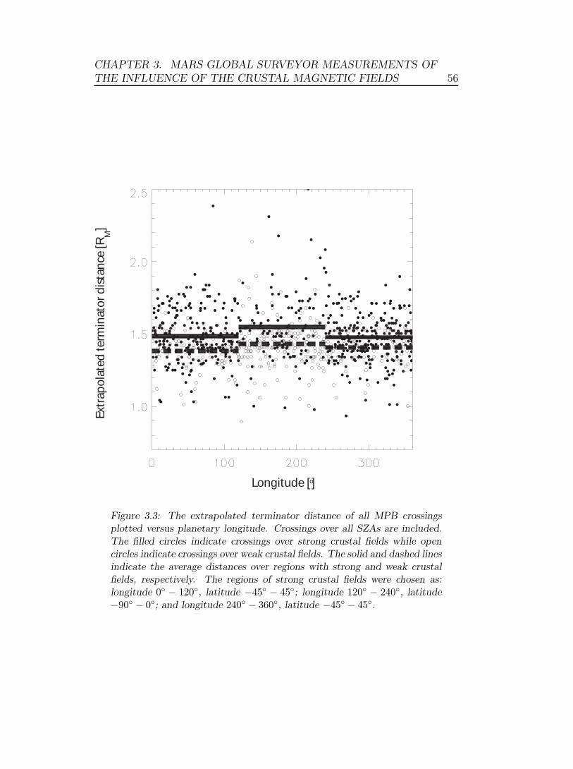
CHAPTER 3. MARS GLOBAL SURVEYOR MEASUREMENTS OFTHE INFLUENCE OF THE CRUSTAL MAGNETIC FIELDS 56
Extr
apo
late
d te
rmin
ato
r dis
tan
ce [R
]
M
Longitude [ ]o
Figure 3.3: The extrapolated terminator distance of all MPB crossingsplotted versus planetary longitude. Crossings over all SZAs are included.The filled circles indicate crossings over strong crustal fields while opencircles indicate crossings over weak crustal fields. The solid and dashed linesindicate the average distances over regions with strong and weak crustalfields, respectively. The regions of strong crustal fields were chosen as:longitude 0◦ − 120◦, latitude −45◦ − 45◦; longitude 120◦ − 240◦, latitude−90◦ − 0◦; and longitude 240◦ − 360◦, latitude −45◦ − 45◦.

CHAPTER 3. MARS GLOBAL SURVEYOR MEASUREMENTS OFTHE INFLUENCE OF THE CRUSTAL MAGNETIC FIELDS 57
over the specific regions where the crustal sources are locally stronger. Brain
et al. (2005) also confirmed that the MPB is located at higher altitudes over
crustal fields by using electron data from the 400 km altitude mapping orbit
and identified time periods when MGS was in or below the sheath region.
Since the altitude of the spacecraft was more or less constant, detection of
sheath electrons implies that the MPB was pushed downward and this was
observed more frequently over regions without strong crustal sources.
The crustal magnetic fields are rotating with the planet and thus intro-
duce a time varying parameter that influences the MPB. If all other factors
that influence the position of the MPB stay constant, the boundary would
move up and down as the planet rotates. The additional magnetic pressure
from the crustal sources pushes the boundary farther out. This cannot be
distinguished from only one orbit, since there are many factors involved, but
on average it can be detected since the other factors, such as solar wind con-
ditions, average out in the statistics. The existence of mini-magnetospheres
has been suggested by Acuna et al. (1998) and Mitchell et al. (2001), and
appear to be likely features of the Martian plasma environment.
In Figure 3.4 we show evidence that the crustal fields also affect the
Martian BS. The extrapolated BS terminator distance is again plotted as a
function of longitude. Only BS crossings that are observed on the dayside of
Mars are included now because there are essentially no nightside BS cross-
ings in the northern hemisphere and we want an even spatial distribution
of BS crossings in the northern and southern hemisphere. The average dis-
tance over the southern and northern hemisphere of Mars is shown in three
longitude ranges. The average distances of the BS crossings observed over
the southern hemisphere in the same three longitudinal sections (the solid
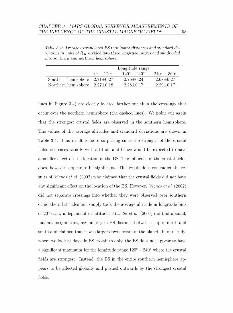
CHAPTER 3. MARS GLOBAL SURVEYOR MEASUREMENTS OFTHE INFLUENCE OF THE CRUSTAL MAGNETIC FIELDS 58
Table 3.4: Average extrapolated BS terminator distances and standard de-viations in units of RM divided into three longitude ranges and subdividedinto southern and northern hemisphere.
Longitude range0◦ − 120◦ 120◦ − 240◦ 240◦ − 360◦
Southern hemisphere 2.71±0.27 2.76±0.24 2.68±0.27Northern hemisphere 2.27±0.18 2.28±0.17 2.29±0.17
lines in Figure 3.4) are clearly located farther out than the crossings that
occur over the northern hemisphere (the dashed lines). We point out again
that the strongest crustal fields are observed in the southern hemisphere.
The values of the average altitudes and standard deviations are shown in
Table 3.4. This result is more surprising since the strength of the crustal
fields decreases rapidly with altitude and hence would be expected to have
a smaller effect on the location of the BS. The influence of the crustal fields
does, however, appear to be significant. This result does contradict the re-
sults of Vignes et al. (2002) who claimed that the crustal fields did not have
any significant effect on the location of the BS. However, Vignes et al. (2002)
did not separate crossings into whether they were observed over southern
or northern latitudes but simply took the average altitude in longitude bins
of 20◦ each, independent of latitude. Mazelle et al. (2004) did find a small,
but not insignificant, asymmetry in BS distance between ecliptic north and
south and claimed that it was larger downstream of the planet. In our study,
where we look at dayside BS crossings only, the BS does not appear to have
a significant maximum for the longitude range 120◦− 240◦ where the crustal
fields are strongest. Instead, the BS in the entire southern hemisphere ap-
pears to be affected globally and pushed outwards by the strongest crustal
fields.
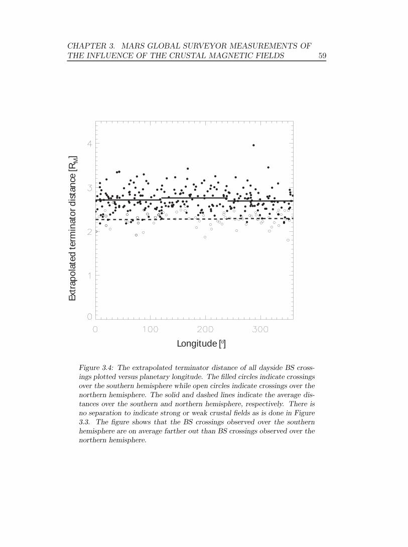
CHAPTER 3. MARS GLOBAL SURVEYOR MEASUREMENTS OFTHE INFLUENCE OF THE CRUSTAL MAGNETIC FIELDS 59
Extr
apo
late
d te
rmin
ato
r dis
tan
ce [R
]
M
Longitude [ ]o
Figure 3.4: The extrapolated terminator distance of all dayside BS cross-ings plotted versus planetary longitude. The filled circles indicate crossingsover the southern hemisphere while open circles indicate crossings over thenorthern hemisphere. The solid and dashed lines indicate the average dis-tances over the southern and northern hemisphere, respectively. There isno separation to indicate strong or weak crustal fields as is done in Figure3.3. The figure shows that the BS crossings observed over the southernhemisphere are on average farther out than BS crossings observed over thenorthern hemisphere.
CHAPTER 3. MARS GLOBAL SURVEYOR MEASUREMENTS OFTHE INFLUENCE OF THE CRUSTAL MAGNETIC FIELDS 60
Dividing the BS crossings into the same regions as the MPB crossings
does not provide the same clear results. The BS crossings in the southern
hemisphere in the longitude range 120◦ − 240◦ are farther out than in the
northern hemisphere in the same longitude range, but the low (< 120◦)
and high (> 240◦) longitude crossings over weak crustal sources are actually
slightly higher in the mid-latitudes. Other factors such as dynamic pressure
or IMF direction seem to be governing in these mid-latitude regions which
could explain the relatively lower BS altitude. It appears as if the BS is not
affected enough by the mid-latitude crustal fields but only by the strongest
crustal fields in the southern hemisphere and there it is being affected over
large scales across the southern hemisphere.
Also, dividing the MPB crossings simply into northern and southern hemi-
sphere crossings gives an insignificant difference in the average distance of
southern and northern crossings in the longitude range from 0◦ to 120◦ as
well as in the longitude range 240◦ − 360◦. This is expected since the strong
crustal sources are located in the mid-latitudes in these longitude ranges and
thus affects the southern and northern hemispheres equally.
The north-south asymmetry of the BS found in this study using MGS
MAG/ER data has been supported by MEX ASPERA-3 measurements (Du-
binin et al., 2008a). They found that in the longitude range 130◦−240◦ in the
southern hemisphere the crustal sources provide essential additional pressure
and lift the MPB upward by 400 − 500 km. The asymmetry in the obsta-
cle shape (the MPB) to the solar wind in turn causes an asymmetry in the
BS location (Dubinin et al., 2008a). A hybrid model simulation of the solar
wind interaction with Mars, which includes the crustal fields, do not show
any global changes in altitude of the BS, whereas the MPB seems to be af-
CHAPTER 3. MARS GLOBAL SURVEYOR MEASUREMENTS OFTHE INFLUENCE OF THE CRUSTAL MAGNETIC FIELDS 61
fected more, and especially over strong crustal sources where it forms more
of a magnetopause-like structure (Harnett and Winglee, 2007).
We have also studied the upstream IMF direction in the 10 min interval
upstream of each crossing, and searched for any preferred orientation that
could explain the north-south asymmetry. However, we do not find any such
IMF orientation for the BS crossings in either of the two hemispheres that
could add to the asymmetry in altitude. It should be said that determining
the orientation of the IMF from the upstream field is difficult. The spacecraft
field can cause errors in the measurements (Crider et al., 2001), and the 10
min averages also introduce an error since the orientation of the field can
change rapidly. Vignes et al. (2002) did indeed find that the upstream IMF
affected the position of the BS but they only used a small portion of the
data points when there was a very steady field orientation. In this study we
use all the data points and not just the ones with a steady upstream IMF
and find that, independent of IMF orientation, the southern BS is almost
always farther out than the northern BS. There does not appear to be any
orbital effect that could account for this asymmetry, either. There are more
BS crossings in the southern hemisphere than in the northern hemisphere
due to orbit geometry but otherwise they do not have any preferred location
relative to the planet that could account for the observed asymmetry in BS
location.
3.2.3 Magnetic field strength at the magnetic pileup
boundary
The MPB is the outer boundary of the MPR which develops as the IMF
drapes around the planet (Nagy et al., 2004). The upper panel of Figure 3.5
CHAPTER 3. MARS GLOBAL SURVEYOR MEASUREMENTS OFTHE INFLUENCE OF THE CRUSTAL MAGNETIC FIELDS 62
shows the mean magnitude of the magnetic field 〈|B|〉 in the inner part of
the MPB (that is the outer part of the MPR) as a function of SZA and the
error bars show the standard deviation of the data σ|B|. The lower panel
shows σ|B| normalized to 〈|B|〉 as a function of SZA so that the relative
values can be seen. The data are binned into 5◦ bins ranging from a SZA
of 25◦ up to 130◦. Brain et al. (2003) examined the relative magnitudes of
the IMF and the planetary crustal field, whereas Crider et al. (2004) studied
only the IMF contribution to the magnitude of the draped field. However,
these studies binned data based on altitude, local time, SZA and geographic
location. Since the plasma environment is highly dynamic and the boundaries
move back and forth with time, that binning method results in data being
taken from different regions of the plasma environment. This study focuses
instead on the field magnitude in the MPB by binning the data after checking
where the MPB is actually located during each orbit. This ensures that we
bin data solely from the boundary region. We use the maximum magnetic
field strength during each MPB crossing in our binning. Crossings that occur
where the crustal field exceeds 5 nT are excluded. This is checked by using the
crustal field model by Cain et al. (2003). As expected, the field magnitude
in Figure 3.5 is higher compared with values obtained in the studies by
Brain et al. (2003) and Crider et al. (2004), by about 25 − 50%, since we
do not sample any sheath magnetic field which is on average lower than the
maximum magnetic field in the MPB. The magnitude of the magnetic field
in the MPB is found to be around 40 nT on the dayside of the planet, and
to decrease almost linearly with SZA towards the nightside where it is on
average around 15 nT. The draped flux tubes within the MPB are thus most
strongly compressed in the subsolar region, as expected, but expand around
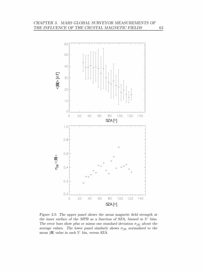
CHAPTER 3. MARS GLOBAL SURVEYOR MEASUREMENTS OFTHE INFLUENCE OF THE CRUSTAL MAGNETIC FIELDS 63
SZA [ ]
SZA [ ]
<|B
|> [n
T]
σ /
<|B
|>
|B|
0
0
Figure 3.5: The upper panel shows the mean magnetic field strength atthe inner surface of the MPB as a function of SZA, binned in 5◦ bins.The error bars show plus or minus one standard deviation σ|B| about theaverage values. The lower panel similarly shows σ|B| normalized to themean |B| value in each 5◦ bin, versus SZA.
CHAPTER 3. MARS GLOBAL SURVEYOR MEASUREMENTS OFTHE INFLUENCE OF THE CRUSTAL MAGNETIC FIELDS 64
the planet into the nightside. While the magnitude of the mean magnetic
field strength decreases towards the nightside, the relative variation of the
field strength actually increases towards the nightside.
In Figure 3.6 the mean field strength variation with altitude within the
dayside MPB is shown in four altitude sections and sub-divided into high
(> 60◦) and low (< 60◦) SZA. The altitude sections are chosen as 0.0 − 0.1
and 0.1 − 0.2 RM above and below the average location of the MPB (the
dashed lines in Figure 3.6 indicate the four regions) and the SZA division is
at an angle of 60◦. The field strength in the MPB is clearly seen to increase
as the MPB moves toward the surface of the planet, implying that when the
solar wind dynamic pressure pushes the boundary closer to the planet the
magnetic flux piled up in front of the planet must be stored in a smaller
volume and the magnetic field strength thus increases. The field strength in
the outer region (higher altitude) is of order 70% of that in the inner region
(lower altitude), for both high and low SZAs.
3.3 Summary and conclusions
We have analyzed the full pre-mapping data set from the MGS MAG and
ER instruments. The study has focused on the shape and location of the
two boundaries as well as on the effects of the crustal magnetic fields on
the location of the MPB and BS. We also study the magnetic field strength
inside the MPB.
The pre-mapping data set contains sixteen months of data with good cov-
erage in SZA, local time, and altitude. We use this to search for crossings
of the MPB and BS and find 993 and 619, respectively. The MPB appears

CHAPTER 3. MARS GLOBAL SURVEYOR MEASUREMENTS OFTHE INFLUENCE OF THE CRUSTAL MAGNETIC FIELDS 65
Y +
Z
22
[R ] M
X [R ]M
<|B|> [nT] σ 20.6 4.223.4 7.427.2 12.531.1 11.0
|B|
<|B|> [nT] σ 31.4 7.931.3 9.635.3 10.243.1 11.8
|B|
Figure 3.6: All dayside MPB crossings are shown in aberrated cylindricalMSO coordinates (crosses), together with the best fit (solid line). Tworegions on either side of this best fit line are then indicated by dashedlines, each region being 0.1 RM wide. The altitude sections are also sub-divided into SZAs less than 60◦ and SZAs larger than 60◦, indicated by thetilted solid line. The average magnetic field strength and their standarddeviations of the MPB crossings observed in each of the eight regions areshown. The upper left value (20.6 nT) is the average magnetic field strengthof the MPB crossings observed in the top region of the large SZA division,etc.
CHAPTER 3. MARS GLOBAL SURVEYOR MEASUREMENTS OFTHE INFLUENCE OF THE CRUSTAL MAGNETIC FIELDS 66
as a permanent boundary in the Martian plasma environment, and is the
boundary where the IMF starts to pile up upstream of the obstacle. Its loca-
tion is to a large extent governed by the pressure balance between magnetic
pressure on the inside and solar wind dynamic pressure on the outside. In
a time series from MGS MAG/ER it is identified by a sudden increase in
magnetic field magnitude together with a drop in field fluctuations as well
as a drop in electron flux. The increase in field magnitude is larger on the
dayside than on the nightside and the scatter in position of the boundary is
more extensive on the nightside.
The shape and location of the MPB and BS are found to be in agreement
with previous studies but with some smaller differences in stand-off distance
and tail radius. We introduce a new fitting technique which gives a more
realistic MPB shape by making sure that the lowest altitude of the boundary
is at the subsolar point.
The crustal fields are shown to play an important role in the location
of the MPB as well as the BS. The additional magnetic pressure from the
crustal sources forces the MPB to higher altitudes over the large scale regions
where there are stronger crustal fields. By extrapolating each MPB crossing
to the terminator line and dividing them into whether they are observed
over regions of weak or strong crustal fields we find that the crossings that
occur over regions with intense crustal magnetic fields are on average located
farther out. We have repeated this division in three longitude ranges and
obtained the same result in all three regions. For the MPB, the extrapolated
terminator distances are on average farthest away in the longitude range
120◦−240◦ within the latitude range from −90◦ to 0◦, which is coincident with
where the strongest crustal fields sources are located. This clear distinction
CHAPTER 3. MARS GLOBAL SURVEYOR MEASUREMENTS OFTHE INFLUENCE OF THE CRUSTAL MAGNETIC FIELDS 67
between weak and strong crustal field regions is not seen for the BS crossings.
This is at least partly expected since the magnitude of the crustal fields falls
off with altitude and it gets more and more disturbed by the surrounding
plasma environment. However, on a global scale the crustal field still appears
to make a large difference since the BS crossings observed over the southern
hemisphere are located significantly farther out than the northern hemisphere
crossings. The BS does not seem to be affected by the intermediate crustal
field strength in the mid-latitude regions and that indicates that there might
be a threshold crustal field strength required to lift the BS. It has not been
possible to relate this asymmetry to any particular upstream IMF orientation
or orbit geometry effect. The observed asymmetry in both the MPB and BS
altitude is supported by measurements from MEX.
The magnetic field strength at the inner edge of the MPB is found to be
about 40 nT on the dayside (no crossings could be observed below a SZA of
20◦ due to orbit constraints), and decreases to about 15 nT on the nightside.
The decrease toward the nightside agrees with what is expected from a gas-
dynamic modelling: as the obstacle surface becomes more tangential to the
solar wind flow, more and more magnetic flux slips by the obstacle and hence
the flux decreases (Spreiter and Stahara, 1980). The flux tubes also expand
downstream of the subsolar point and the field magnitude thus decreases.
The variation in field strength is quite large and the uncertainty of the average
values becomes large. The field strength is shown to increase rapidly with
decreasing altitude. A MPB crossing observed closer to the planet implies,
in general, a larger magnetic field strength in the MPB and a MPB crossings
observed at higher altitude implies smaller field strength.
Chapter 4Rosetta and Mars Express
simultaneous measurements of the
effects of low and high solar wind
pressure
In this Chapter we analyze the measurements made by the Rosetta spacecraft
during its swingby of Mars together with the simultaneous measurements
made by MEX. The data analysis is divided into two parts. First, we perform
a two-spacecraft near-simultaneous plasma boundary study at Mars by using
both Rosetta and MEX measurements during quiet solar wind conditions.
Secondly, we examine the effects of a high pressure solar wind region on
the Martian plasma environment by using Rosetta as a solar wind monitor
while MEX samples the plasma environment over several days. Some of the
material presented in this Chapter is published in Edberg et al. (2009c) and
included in Edberg et al. (2009a).
68
CHAPTER 4. ROSETTA AND MARS EXPRESS SIMULTANEOUSMEASUREMENTS OF THE EFFECTS OF LOW AND HIGH SOLARWIND PRESSURE 69
4.1 Introduction
As the Rosetta spacecraft performed a flyby of Mars on February 25, 2007,
the rare event of a two-spacecraft investigation of the Martian plasma envi-
ronment, together with MEX, became possible. Out of all the past missions
to Mars, with plasma instruments onboard, only two have been in operation
at the same time: MGS and MEX. Results from a study using MGS and
MEX are presented in Chapter 5.
Hence, the Rosetta Mars flyby is the first opportunity for coordinated
plasma measurements near the Martian BS and MPB. The Rosetta and MEX
trajectories during the Mars flyby are presented in Figure 2.3 as blue and
red lines, respectively.
4.2 Simultaneous observations during low so-
lar wind pressure
To enable us to find the locations of the BS, MPB and PEB, which are our
prime targets in this study, Figure 4.1 shows the Rosetta ROMAP magnetic
field data from the inbound leg of the Rosetta Mars flyby. Data are shown
as total field strength and x, y and z-components in MSO coordinates. The
expected crustal magnetic field strength from a model by Cain et al. (2003)
is also shown as well as the altitude of Rosetta. For the outbound leg, a sum-
mary of RPC data are shown in Figure 4.3. The MEX measurements during
this interval are presented in Figure 4.4. These plots form the basic material
for the following Sections where we will first describe the Rosetta plasma
boundary crossings and then the simultaneously occurring MEX boundary
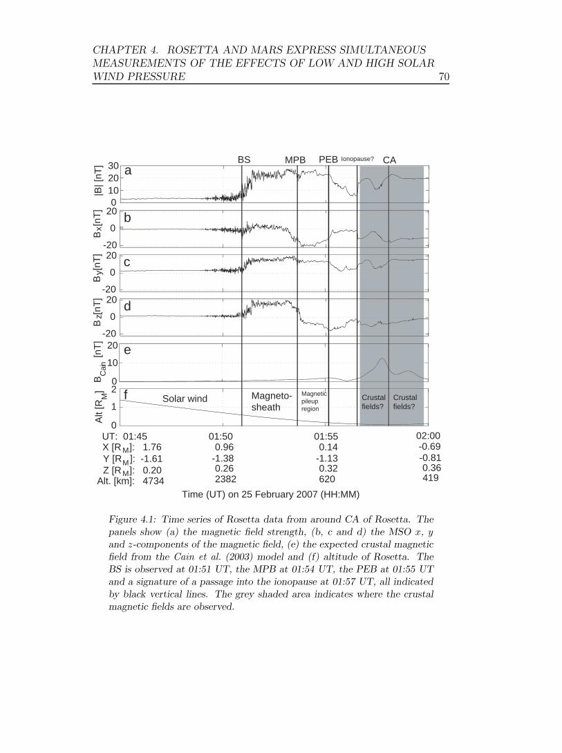
CHAPTER 4. ROSETTA AND MARS EXPRESS SIMULTANEOUSMEASUREMENTS OF THE EFFECTS OF LOW AND HIGH SOLARWIND PRESSURE 70
0102030
|B| [
nT]
-20
0
20
B [
nT]
0
10
20
BC
ain [n
T]
UT: 01:45 01:50 01:55 02:000
1
2
Time (UT) on 25 February 2007 (HH:MM)
Alt
[RM
]
BS MPB
Magnetic pileup region
Magneto-sheath
Solar wind
a
d
e
f
X [R ]: 1.76 0.96 0.14 -0.69-1.38 -1.13 -0.810.26 0.32 0.36
M Y [R ]: -1.61M Z [R ]: 0.20M
2382 620Alt. [km]: 4734 419
-20
0
20
B [
nT]
c
-20
0
20
B [
nT]
b
xy
z
Ionopause?
Crustal fields?
CAPEB
Crustal fields?
Figure 4.1: Time series of Rosetta data from around CA of Rosetta. Thepanels show (a) the magnetic field strength, (b, c and d) the MSO x, yand z-components of the magnetic field, (e) the expected crustal magneticfield from the Cain et al. (2003) model and (f) altitude of Rosetta. TheBS is observed at 01:51 UT, the MPB at 01:54 UT, the PEB at 01:55 UTand a signature of a passage into the ionopause at 01:57 UT, all indicatedby black vertical lines. The grey shaded area indicates where the crustalmagnetic fields are observed.
CHAPTER 4. ROSETTA AND MARS EXPRESS SIMULTANEOUSMEASUREMENTS OF THE EFFECTS OF LOW AND HIGH SOLARWIND PRESSURE 71
crossings.
4.2.1 Dayside bow shock crossing
The increased magnetic field strength and level of turbulence occurring in
a wide interval around 01:51 UT (Figure 4.1, panel a - d) is identified as
the BS. The upstream IMF in Figure 4.1 has a field strength of ∼2 nT and
is directed slightly tailward and toward the positive y-hemisphere and to-
ward ecliptic north, which is in agreement with the normal Parker spiral
configuration. With some caution for possible magnetic field offsets, this
magnetic field direction together with the flyby geometry (Figure 2.3) sug-
gests that we should encounter a quasi-parallel BS, (the θBn angle, i.e. the
angle between the IMF and the normal to the BS, is close to 0). While the
separation into quasi-parallel and quasi-perpendicular shocks is less relevant
for Mars than for Earth for several reasons (e.g. small obstacle scale size
with respect to the ion gyro radius and substantial exospheric ionization, see
Mazelle et al. (2004) for a review), a quasi-parallel shock nature is indeed
consistent with the gradual increase in magnetic field strength seen around
01:51 UT, which we will see contrasts drastically to what we observe on the
outbound leg (Section 4.2.4). The fluctuations seen from around 01:49 UT
cannot be taken as an indication of interaction of the solar wind with back
streaming ions upstream of a quasi-parallel shock as such activity at Mars is
found also upstream of the quasi-perpendicular BS, presumably because of
the ionization of exospheric neutrals (Mazelle et al., 2004).
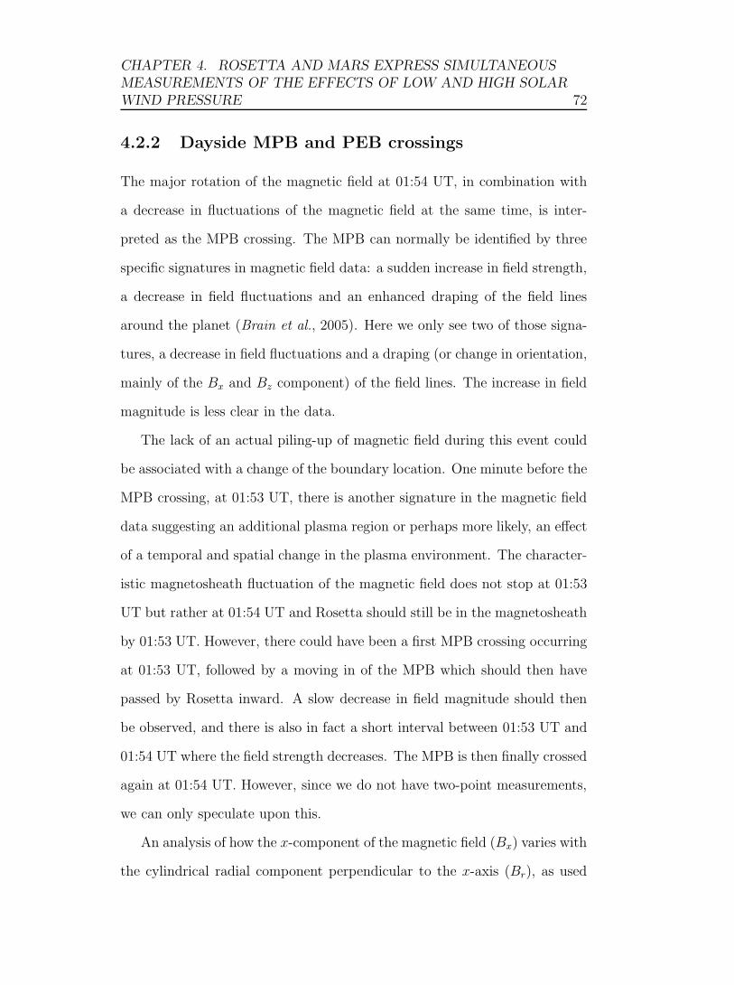
CHAPTER 4. ROSETTA AND MARS EXPRESS SIMULTANEOUSMEASUREMENTS OF THE EFFECTS OF LOW AND HIGH SOLARWIND PRESSURE 72
4.2.2 Dayside MPB and PEB crossings
The major rotation of the magnetic field at 01:54 UT, in combination with
a decrease in fluctuations of the magnetic field at the same time, is inter-
preted as the MPB crossing. The MPB can normally be identified by three
specific signatures in magnetic field data: a sudden increase in field strength,
a decrease in field fluctuations and an enhanced draping of the field lines
around the planet (Brain et al., 2005). Here we only see two of those signa-
tures, a decrease in field fluctuations and a draping (or change in orientation,
mainly of the Bx and Bz component) of the field lines. The increase in field
magnitude is less clear in the data.
The lack of an actual piling-up of magnetic field during this event could
be associated with a change of the boundary location. One minute before the
MPB crossing, at 01:53 UT, there is another signature in the magnetic field
data suggesting an additional plasma region or perhaps more likely, an effect
of a temporal and spatial change in the plasma environment. The character-
istic magnetosheath fluctuation of the magnetic field does not stop at 01:53
UT but rather at 01:54 UT and Rosetta should still be in the magnetosheath
by 01:53 UT. However, there could have been a first MPB crossing occurring
at 01:53 UT, followed by a moving in of the MPB which should then have
passed by Rosetta inward. A slow decrease in field magnitude should then
be observed, and there is also in fact a short interval between 01:53 UT and
01:54 UT where the field strength decreases. The MPB is then finally crossed
again at 01:54 UT. However, since we do not have two-point measurements,
we can only speculate upon this.
An analysis of how the x-component of the magnetic field (Bx) varies with
the cylindrical radial component perpendicular to the x-axis (Br), as used
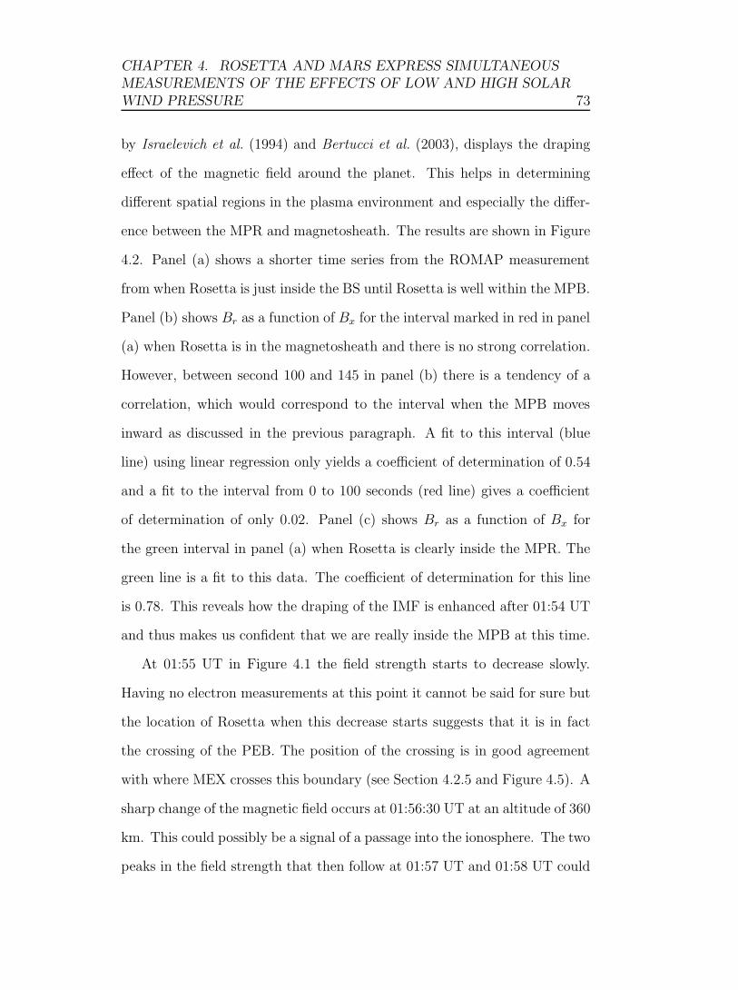
CHAPTER 4. ROSETTA AND MARS EXPRESS SIMULTANEOUSMEASUREMENTS OF THE EFFECTS OF LOW AND HIGH SOLARWIND PRESSURE 73
by Israelevich et al. (1994) and Bertucci et al. (2003), displays the draping
effect of the magnetic field around the planet. This helps in determining
different spatial regions in the plasma environment and especially the differ-
ence between the MPR and magnetosheath. The results are shown in Figure
4.2. Panel (a) shows a shorter time series from the ROMAP measurement
from when Rosetta is just inside the BS until Rosetta is well within the MPB.
Panel (b) shows Br as a function of Bx for the interval marked in red in panel
(a) when Rosetta is in the magnetosheath and there is no strong correlation.
However, between second 100 and 145 in panel (b) there is a tendency of a
correlation, which would correspond to the interval when the MPB moves
inward as discussed in the previous paragraph. A fit to this interval (blue
line) using linear regression only yields a coefficient of determination of 0.54
and a fit to the interval from 0 to 100 seconds (red line) gives a coefficient
of determination of only 0.02. Panel (c) shows Br as a function of Bx for
the green interval in panel (a) when Rosetta is clearly inside the MPR. The
green line is a fit to this data. The coefficient of determination for this line
is 0.78. This reveals how the draping of the IMF is enhanced after 01:54 UT
and thus makes us confident that we are really inside the MPB at this time.
At 01:55 UT in Figure 4.1 the field strength starts to decrease slowly.
Having no electron measurements at this point it cannot be said for sure but
the location of Rosetta when this decrease starts suggests that it is in fact
the crossing of the PEB. The position of the crossing is in good agreement
with where MEX crosses this boundary (see Section 4.2.5 and Figure 4.5). A
sharp change of the magnetic field occurs at 01:56:30 UT at an altitude of 360
km. This could possibly be a signal of a passage into the ionosphere. The two
peaks in the field strength that then follow at 01:57 UT and 01:58 UT could
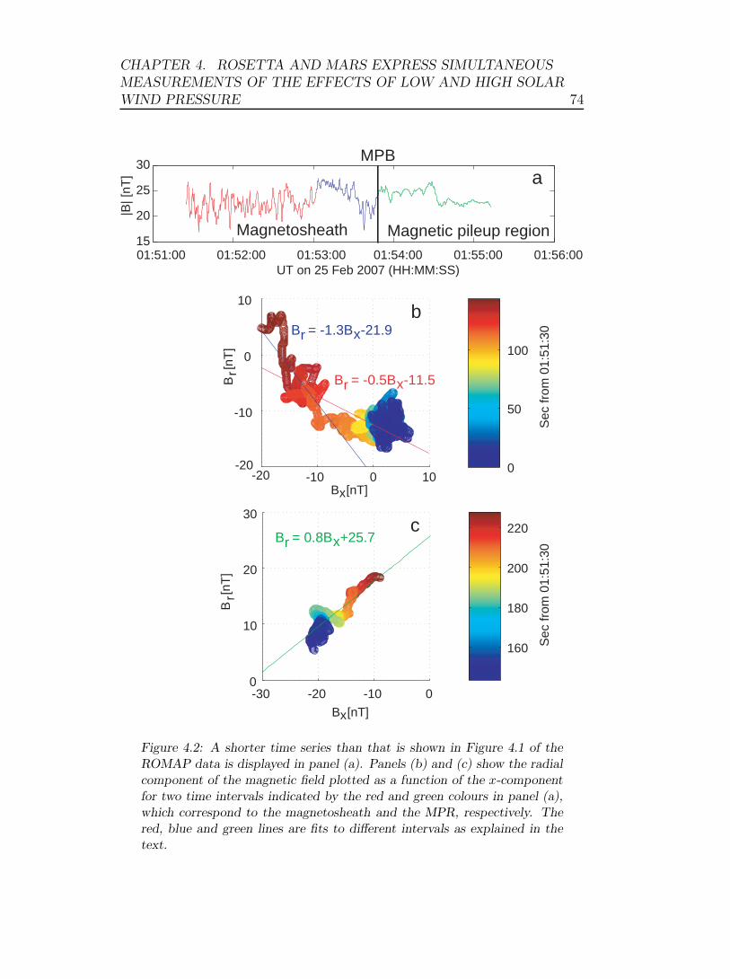
CHAPTER 4. ROSETTA AND MARS EXPRESS SIMULTANEOUSMEASUREMENTS OF THE EFFECTS OF LOW AND HIGH SOLARWIND PRESSURE 74
01:51:00 01:52:00 01:53:00 01:54:00 01:55:00 01:56:0015
20
25
30
UT on 25 Feb 2007 (HH:MM:SS)
|B| [
nT]
-20 -10 0 10-20
-10
0
10
B [nT]
B [
nT]
0
50
100
-30 -20 -10 00
10
20
30
B [nT]
B [
nT]
160
180
200
220
a
b
cS
ec fr
om 0
1:51
:30
Sec
from
01:
51:3
0B = 0.8B +25.7r x
B = -1.3B -21.9r x
B = -0.5B -11.5r x
rr
x
x
Magnetosheath Magnetic pileup region
MPB
Figure 4.2: A shorter time series than that is shown in Figure 4.1 of theROMAP data is displayed in panel (a). Panels (b) and (c) show the radialcomponent of the magnetic field plotted as a function of the x-componentfor two time intervals indicated by the red and green colours in panel (a),which correspond to the magnetosheath and the MPR, respectively. Thered, blue and green lines are fits to different intervals as explained in thetext.

CHAPTER 4. ROSETTA AND MARS EXPRESS SIMULTANEOUSMEASUREMENTS OF THE EFFECTS OF LOW AND HIGH SOLARWIND PRESSURE 75
be signatures of crustal magnetic fields. Looking at the crustal field model
by Cain et al. (2003), the two peaks observed in the ROMAP data are close
to what is expected, except for a short time difference of about 1 minute,
which may well be due to plasma effects which are specifically excluded from
the Cain model. The Cain model was restricted to only use data from below
200 km altitude and only from the dayside. The measured magnetic field
is a combination of draped IMF and crustal fields and hence the magnitude
of the Cain model is expected to be less than the measured values. Even
though the morphologies of these signatures are somewhat different from
what was measured by MGS we believe that it is likely that these are indeed
crustal magnetic fields. Boesswetter et al. (2009) used the second version of
the crustal field model from (Purucker et al., 2000) and also found a clear
crustal magnetic field signature in the de-trended ROMAP data.
4.2.3 Flank MPB crossing
Figure 4.3 shows a time series of measurements by the Rosetta IES, MAG
and LAP instruments on the outbound leg from 02:55 UT, just after the
payload turn-on following the shut-down period around CA, until 04:30 UT.
The altitude above Mars and the spacecraft SAA are also displayed in the
Figure. The SAA is of interest as it determines the perturbation on the
LAP Vps measurement from the solar panels, and also determines if the solar
wind enters the IES field of view. The density data in panel (f) in Figure
4.3 was produced by using the calibration function between Rosetta LAP
and MEX ELS as described in Edberg et al. (2009c). The IES instrument
was behind the spacecraft (with respect to the solar wind flow) during this
interval and thus did not see the entire distribution of streaming solar wind
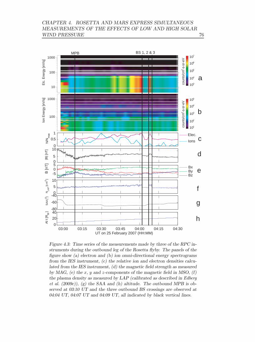
CHAPTER 4. ROSETTA AND MARS EXPRESS SIMULTANEOUSMEASUREMENTS OF THE EFFECTS OF LOW AND HIGH SOLARWIND PRESSURE 76
coun
ts/c
m2 -s
-sr-
eV
101
102
103
104
105
coun
ts/c
m2 -s
-sr-
eV
103
104
105
106
107
100
1000
Ion
Ene
rgy
[eV
/q]
10
100
1000
Elc
. Ene
rgy
[eV
/q]
0
0.5
1
N/N
max
05
10
|B| [
nT]
-505
B [n
T]
0
5
10
NLA
P [c
m -3
]
-80
-60 -40
SA
A [0 ]
03:00 03:15 03:30 03:45 04:00 04:15 04:300
20
40
Al t
[R M
]
UT on 25 February 2007 (HH:MM)
Ions
Elec.
BxByBz
MPB BS 1, 2 & 3
a
b
c
d
e
g
f
h
Figure 4.3: Time series of the measurements made by three of the RPC in-struments during the outbound leg of the Rosetta flyby. The panels of thefigure show (a) electron and (b) ion omni-directional energy spectrogramsfrom the IES instrument, (c) the relative ion and electron densities calcu-lated from the IES instrument, (d) the magnetic field strength as measuredby MAG, (e) the x, y and z-components of the magnetic field in MSO, (f)the plasma density as measured by LAP (calibrated as described in Edberget al. (2009c)), (g) the SAA and (h) altitude. The outbound MPB is ob-served at 03:10 UT and the three outbound BS crossings are observed at04:04 UT, 04:07 UT and 04:09 UT, all indicated by black vertical lines.
CHAPTER 4. ROSETTA AND MARS EXPRESS SIMULTANEOUSMEASUREMENTS OF THE EFFECTS OF LOW AND HIGH SOLARWIND PRESSURE 77
and magnetosheath particles. For IES, we therefore only present the relative
changes in the ion and electron number density, from density moments of
the ion and electron distribution. While the flowing ions are hidden from
the instrument, the electrons have higher thermal speed and can more easily
reach the instrument, giving a more reliable density moment. The IES energy
spectrograms changes energy resolution at about 03:03 UT which is clearly
seen in the data. After this change, the electron and ion fluxes are seen
to drop sharply at 60 eV since the first energy channels goes up to this
energy level. Both spectrograms were generated by summing counts over all
elevations and azimuth angles and hence the direction information is lost in
the energy spectrogram. It should be noted that there is good covariation
between the LAP and IES electron density variations, giving confidence in
the measurements.
The Rosetta trajectory was close to tangential to the plasma boundaries
during the outbound leg. This may explain the gradual magnetic field gradi-
ent at the start of the interval, which we interpret as a stretched MPB. We
note that the significant change at 03:02 UT is likely to be an artefact intro-
duced by the changing attitude. The MPB position is thus not fully clear,
but on moving from inside the MPB to outside, the decrease in magnetic
field magnitude is gradual but with a distinct minimum at 03:10 UT where
there is again a rotation of the field direction, an effect of the IMF draping
around the obstacle, and we therefore identify this as the MPB.
4.2.4 Flank magnetosheath and bow shock crossings
Throughout the first hour in Figure 4.3, there is a gradual increase in the Vps
which has been translated to number density NLAP (Figure 4.3, panel (f))
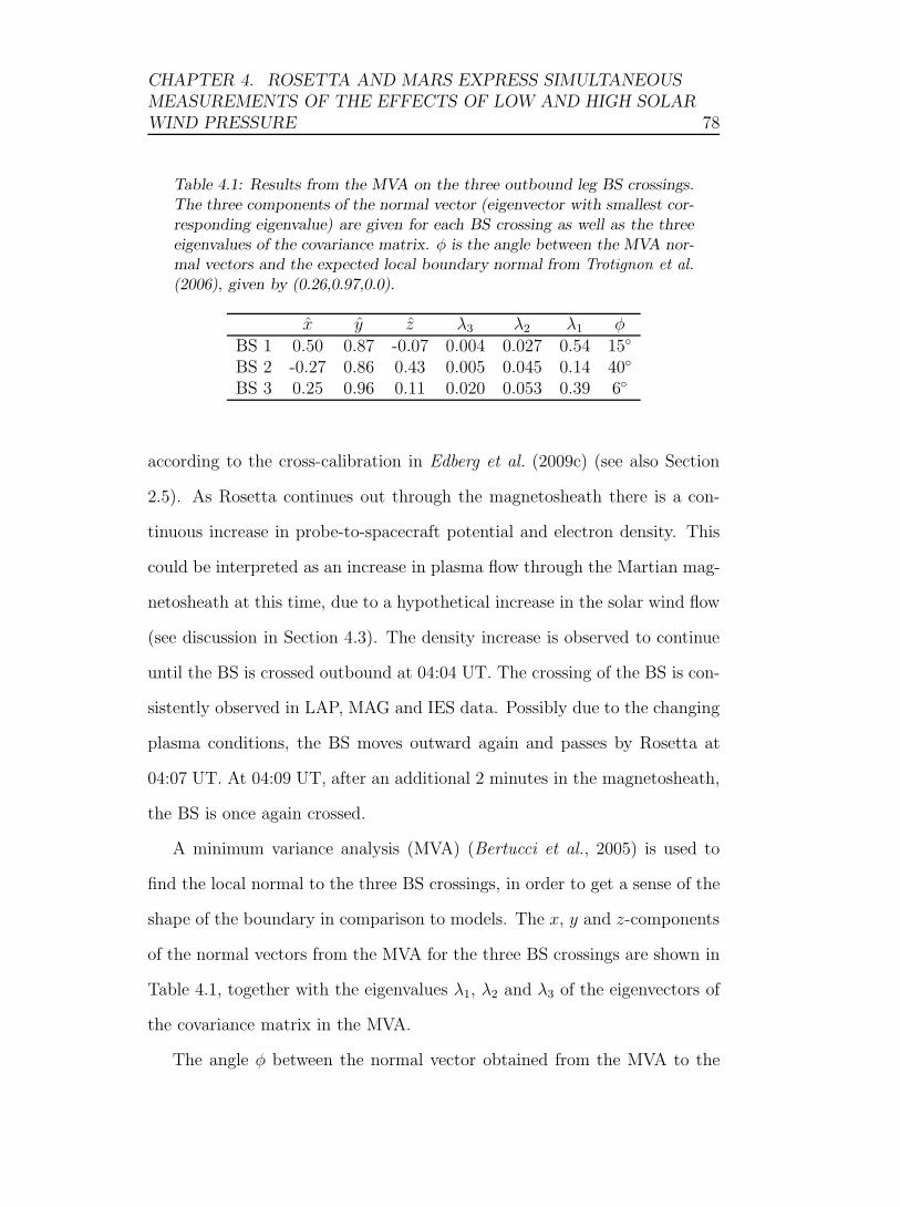
CHAPTER 4. ROSETTA AND MARS EXPRESS SIMULTANEOUSMEASUREMENTS OF THE EFFECTS OF LOW AND HIGH SOLARWIND PRESSURE 78
Table 4.1: Results from the MVA on the three outbound leg BS crossings.The three components of the normal vector (eigenvector with smallest cor-responding eigenvalue) are given for each BS crossing as well as the threeeigenvalues of the covariance matrix. φ is the angle between the MVA nor-mal vectors and the expected local boundary normal from Trotignon et al.(2006), given by (0.26,0.97,0.0).
x y z λ3 λ2 λ1 φBS 1 0.50 0.87 -0.07 0.004 0.027 0.54 15◦
BS 2 -0.27 0.86 0.43 0.005 0.045 0.14 40◦
BS 3 0.25 0.96 0.11 0.020 0.053 0.39 6◦
according to the cross-calibration in Edberg et al. (2009c) (see also Section
2.5). As Rosetta continues out through the magnetosheath there is a con-
tinuous increase in probe-to-spacecraft potential and electron density. This
could be interpreted as an increase in plasma flow through the Martian mag-
netosheath at this time, due to a hypothetical increase in the solar wind flow
(see discussion in Section 4.3). The density increase is observed to continue
until the BS is crossed outbound at 04:04 UT. The crossing of the BS is con-
sistently observed in LAP, MAG and IES data. Possibly due to the changing
plasma conditions, the BS moves outward again and passes by Rosetta at
04:07 UT. At 04:09 UT, after an additional 2 minutes in the magnetosheath,
the BS is once again crossed.
A minimum variance analysis (MVA) (Bertucci et al., 2005) is used to
find the local normal to the three BS crossings, in order to get a sense of the
shape of the boundary in comparison to models. The x, y and z-components
of the normal vectors from the MVA for the three BS crossings are shown in
Table 4.1, together with the eigenvalues λ1, λ2 and λ3 of the eigenvectors of
the covariance matrix in the MVA.
The angle φ between the normal vector obtained from the MVA to the

CHAPTER 4. ROSETTA AND MARS EXPRESS SIMULTANEOUSMEASUREMENTS OF THE EFFECTS OF LOW AND HIGH SOLARWIND PRESSURE 79
expected boundary normal from Trotignon et al. (2006) is also shown. During
the first and third crossings on the outbound leg, the normal direction is very
close to parallel to the local normal to the conic section, assumed to represent
the average surface boundary (Trotignon et al., 2006), in the x−y plane and
with a small z-component, which is expected. However, for the second of the
three outbound BS crossings, the normal obtained from the MVA analysis is
tilted in the downstream direction and with a larger z-component, suggesting
that the BS moved outwards in a wave motion propagating downstream. We
note that the magnetic field direction in the solar wind (Figure 4.3) and the
BS normal directions at the two outbound crossings are consistent with a
quasi-perpendicular BS. This is also indicated by the discontinuous nature of
the observed BS crossings, in distinct contrast to the dayside BS (Figure 4.1).
However, as discussed in Section 4.2.1, the smeared-out nature of the inbound
BS may be more due to its proximity to the planet, putting it inside the
Martian exosphere, rather than to the effects of its normal direction with
respect to the IMF (Mazelle et al., 2004).
4.2.5 Mars Express observations
The MEX orbit on February 25, 2007, was close to the terminator plane
with periapsis of ∼310 km altitude in the +y/-z-hemisphere and apoapsis
of about ∼10000 km altitude in the -y/+z-hemisphere. A time series of the
ion and electron measurements from IMA and ELS at this time is plotted in
Figure 4.4 together with the velocity and density moments. The solar wind
is slightly slower than average at this time, below 300 km s−1, with a density
of ∼1-2 cm−3. Meanwhile, the ROMAP data from Rosetta indicates that the
IMF strength is quite ordinary and aligned with the expected Parker spiral
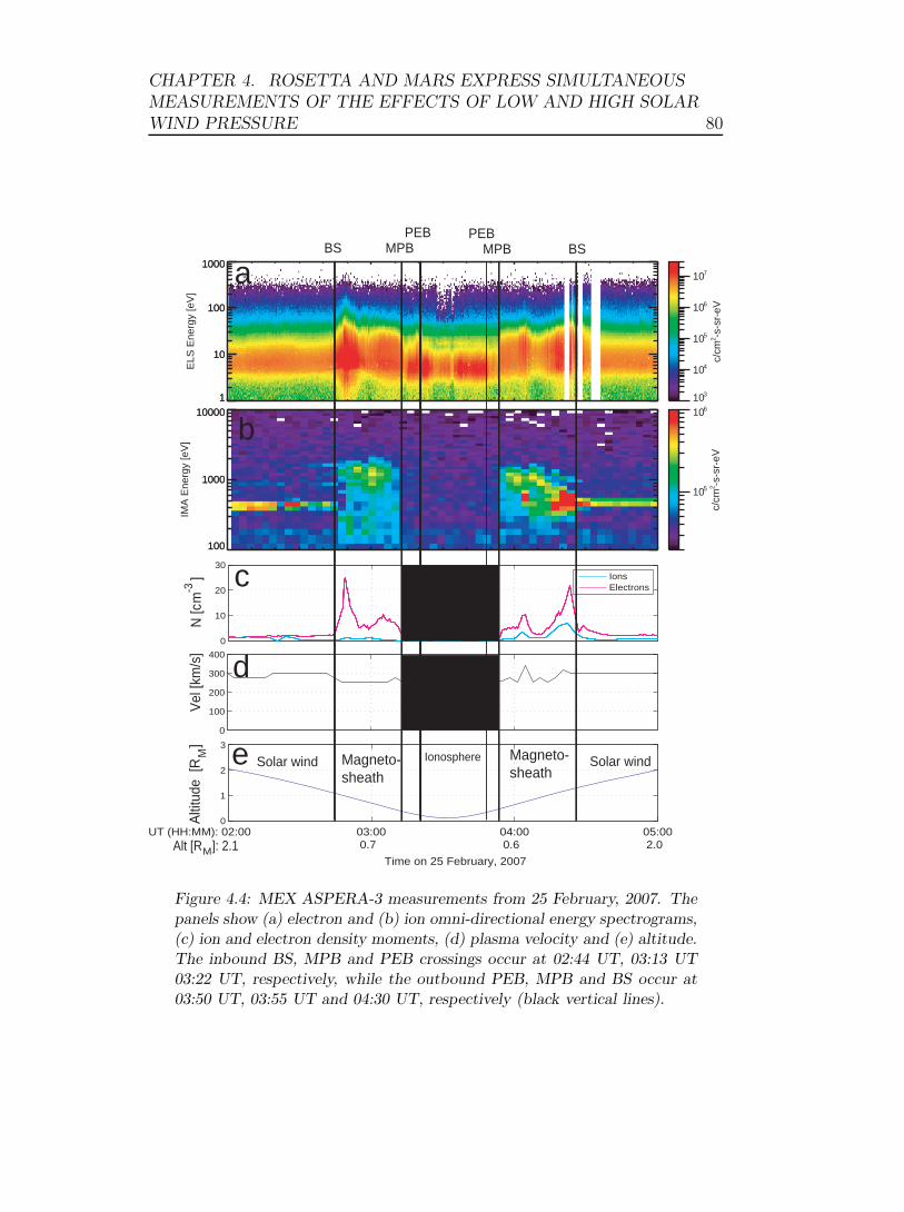
CHAPTER 4. ROSETTA AND MARS EXPRESS SIMULTANEOUSMEASUREMENTS OF THE EFFECTS OF LOW AND HIGH SOLARWIND PRESSURE 80
BS BSMPB MPBPEB?PEB?
0
10
20
30
N [c
m-3
]
0
100
200
300
400
Vel
[km
/s]
UT (HH:MM): 02:00 03:00 04:00 05:000
1
2
3
Time on 25 February, 2007
Alti
tude
[R
M]
IonsElectrons
Solar wind Solar windMagneto-sheath
Magneto-sheath
Ionosphere
c
d
e
10
10
10
10
10
10
10 1
10
100
1000
ELS
Ene
rgy
[eV
]
1
10
100
1000
3
4
5
6
7
c/cm
2 -s-s
r-eV
100
1000
10000
IMA
Ene
rgy
[eV
]
100
1000
10000
5
6
c/cm
2 -s-s
r-eV
BS BSMPB MPBPEBPEB
a
b
Alt [R ]: 2.1 0.7 0.6 2.0M
Figure 4.4: MEX ASPERA-3 measurements from 25 February, 2007. Thepanels show (a) electron and (b) ion omni-directional energy spectrograms,(c) ion and electron density moments, (d) plasma velocity and (e) altitude.The inbound BS, MPB and PEB crossings occur at 02:44 UT, 03:13 UT03:22 UT, respectively, while the outbound PEB, MPB and BS occur at03:50 UT, 03:55 UT and 04:30 UT, respectively (black vertical lines).
CHAPTER 4. ROSETTA AND MARS EXPRESS SIMULTANEOUSMEASUREMENTS OF THE EFFECTS OF LOW AND HIGH SOLARWIND PRESSURE 81
direction, see Section 4.2. During the inbound crossing of the BS and the
MPB by Rosetta at 1:51 UT and 1:53 UT, respectively, MEX was in the
solar wind. Figure 4.4 shows that the solar wind was quiet for a long period
before the Rosetta CA at 01:58. Based on the MEX observations it is rea-
sonable to assume that the upstream conditions during the Rosetta inbound
leg were constant. Rosetta ROMAP data (Figure 4.1) and Rosetta MAG
data (Figure 4.3) show that the IMF has changed sign of the z-component
from before the flyby until after the flyby, while the field strength has not
changed significantly.
During the full orbit of MEX, the spacecraft encountered several regions
and boundaries in the Martian plasma environment, as can be seen in Figure
4.4. First, MEX was in the solar wind until 02:44 UT when the spacecraft
crossed the BS, and was thereafter located in the Martian magnetosheath.
The magnetosheath was clearly identified by the appearance of solar wind
electrons heated at the BS crossing. A similar signature was observed in the
ion spectrogram. At 03:13 UT a significant change in the ion and electron
fluxes occurred. The sudden disappearance of magnetosheath electrons is
interpreted as a crossing of the MPB. At 03:22 UT the PEB is crossed,
detected in the ELS data by the appearance of a spectral line at energy
of 20 - 30 eV. MEX stayed inside the Martian PEB for 28 minutes, until
03:50 UT when the spacecraft crossed the PEB outbound. The MPB was
crossed outbound at 03:55 UT and again the magnetosheath was entered
before finally the solar wind region was reached after having crossed the BS
at 04:30 UT.
CHAPTER 4. ROSETTA AND MARS EXPRESS SIMULTANEOUSMEASUREMENTS OF THE EFFECTS OF LOW AND HIGH SOLARWIND PRESSURE 82
4.3 Shape and location of the plasma bound-
aries
The positions and times of all MPB, PEB and BS crossings observed by
Rosetta and MEX, as reported in the previous sections, are indicated in
Figure 4.5, on two different scales. Also shown are the orbits of MEX and
Rosetta in cylindrical MSO coordinates and the average BS and MPB loca-
tions from Trotignon et al. (2006) plotted as solid green and red lines. We use
the model of Trotignon et al. (2006) since it has been specifically developed
to model the boundaries far downstream which is where we have some of our
boundary crossings in this study. The dashed green line is a conic section fit
to the three BS crossings closest to the planet that were observed by both
Rosetta and MEX and the dashed blue line is a fit to the three PEB cross-
ings. The inbound MPB crossing by MEX and the outbound MPB crossing
by Rosetta are only separated by 3 minutes in time. The outbound BS cross-
ing by Rosetta is observed approximately 20 minutes before the outbound BS
crossing of MEX. This makes these measurements the first near-simultaneous
two-spacecraft measurement of plasma boundaries at Mars. The observations
of the PEB by Rosetta and MEX are separated 1.5 hours in time making
them far from simultaneous. The time-scales on which these three bound-
aries move significantly can be anything between a couple of seconds up to
perhaps hours depending on solar wind variability. During the time off the
Rosetta flyby the solar wind conditions are steady and slow, when observed
by either of the two spacecraft. What happens to the solar wind during the
time when both spacecraft are inside the BS is unknown, but considering
the stable situation before and after this interval, a reasonable assumption

CHAPTER 4. ROSETTA AND MARS EXPRESS SIMULTANEOUSMEASUREMENTS OF THE EFFECTS OF LOW AND HIGH SOLARWIND PRESSURE 83
Figure 4.5: The trajectories of Rosetta and MEX on 25 February 2007plotted in cylindrical MSO coordinates and shown in two scale sizes. Thegreen and red solid curves are the average positions of the BS and MPBfrom Trotignon et al. (2006). The positions of the boundary crossingsobserved by Rosetta and MEX are displayed as green (BS), red (MPB)and blue (PEB) stars and plus signs. Stars refer to Rosetta observationsand plus signs to MEX. The time, in UT, of each crossing is also indicated.The dashed green line is a fit to the three BS crossings closest to the planet(see text for further details on the fitting) and the blue dashed line is a fitto the PEB crossings.

CHAPTER 4. ROSETTA AND MARS EXPRESS SIMULTANEOUSMEASUREMENTS OF THE EFFECTS OF LOW AND HIGH SOLARWIND PRESSURE 84
is that the solar wind does not vary very much, except for a change in the
sign of Bz. However, this leaves unexplained the observed continuous den-
sity increase (as indicated from the probe potential measurements and also to
some extent from the IES electron moment) seen during the outward passage
through the magnetosheath (Figure 4.3 and Section 4.2.4). There is of course
the possibility of a short-time change in the solar wind in the time-interval
between the last Rosetta MPB crossing and the last Rosetta BS crossing
which could cause the density increase. The increase is less than a factor of
two in NLAP which is within the error margins of the density calibration so
there is also the possibility of the increase being unphysical. However, even
though the calibration has an error margin, the individual Vps measurements
should not have a time-dependent error that would cause a factor of two
increase over about one hour, which suggests that the increase is indeed real.
There is also a simultaneous increase in the magnetic field strength at this
time which supports the interpretation of this being physical.
We compare our measurements of the MPB and BS with previous models
of the shape of the two boundaries. For the BS, a conic section is fitted to
the three farthest upstream BS crossings (dashed curve in Figure 4.5). The
fitting is done by altering the semi-latus rectum of the conic section from the
best fit value of Trotignon et al. (2006) until the root mean square of the
distances from each BS crossing to the proposed fit reaches a minimum, as
described in Section 3.2.2. However, this fit does not agree with the farthest
downstream BS crossing. This suggests that the shape of the BS may well
be represented by a conic section but the entire boundary does not seem to
move like a rigid body but rather alters its shape somewhat. In this case, it
becomes more compressed in the far downstream region. For the MPB on
CHAPTER 4. ROSETTA AND MARS EXPRESS SIMULTANEOUSMEASUREMENTS OF THE EFFECTS OF LOW AND HIGH SOLARWIND PRESSURE 85
the other hand, all crossings are reasonably close to the average position of
the boundary, even far back in the tail. The PEB fit is done assuming that
the boundary has the same shape as the MPB on the dayside.
The location of the BS at this time differs from the average location. The
entire BS seems, based upon point measurements, to be compressed during
these 2.5 hours even though the solar wind speed is slow and the density
moderate. This may seem unexpected since an increase in dynamic pressure
should cause the boundary to be pushed farther inward.
It has been shown by Mazelle et al. (2004) and Edberg et al. (2008) that
the dayside BS is on average closer over the northern hemisphere of Mars
than it is over the southern hemisphere by about 0.4 RM , presumably due
to the influence of the crustal magnetic field. This is in agreement with the
location of the inbound Rosetta BS crossing and the outbound MEX BS
crossing, which are both observed in the northern hemisphere. The inbound
MEX BS crossing, which is observed in the southern hemisphere, is still
closer in than average but is the most distant crossing of these three. It is
however only about 0.2 RM farther out than the other two, if extrapolated to
the terminator plane. The crossing by Rosetta far down tail is also located
farther in than average but is observed close to the orbital plane of Mars and
at a large distance in the y-direction.
The location of the MPB is found close to its average position at all times
during the Rosetta flyby which indicates that it is not governed by the same
factors (such as solar wind dynamic pressure and IMF orientation) as the
BS, or at least does not move on the same timescales when a change of these
factors occur, considering that the BS is compressed during the entire flyby
interval.
CHAPTER 4. ROSETTA AND MARS EXPRESS SIMULTANEOUSMEASUREMENTS OF THE EFFECTS OF LOW AND HIGH SOLARWIND PRESSURE 86
4.4 Simultaneous observations during high pres-
sure solar wind
Rosetta only stayed within the Martian plasma environment for a couple
of hours when it could perform simultaneous in situ measurements together
with MEX, which we have focused on in the previous Sections. However, the
plasma instruments on Rosetta were switched on for 5 days around the time
of the flyby, which enabled further possibilities in terms of two-spacecraft
studies at Mars. In the following Sections we will present a study where we
use Rosetta as a solar wind monitor while MEX samples the Martian plasma
environment in order to study the influence of high solar wind dynamic pres-
sure on the plasma boundaries around Mars.
The orbit geometry of MEX and Rosetta is shown in Figure 4.6 for a
longer interval during the time of the Rosetta Mars swingby. Also shown
are the positions of all the MPB and BS crossings as observed by MEX
from 00 UT on 24 February 2007 until 24 UT on 27 February 2007 together
with empirical models of the two boundaries from Edberg et al. (2008) and
Trotignon et al. (2006). The position of each crossing, which are identified
in the ELS data, is adjusted to account for the mean 4◦ aberration of the
solar wind direction caused by the orbital motion of the planet while the
MEX orbit (black solid line) is not adjusted. Note that the inbound and
the outbound boundary crossings occurred on almost opposite sides of the
planet. MEX was at this time, as stated previously, in an elliptical 6-hour
orbit very close to the terminator plane of Mars. It hence crossed the MPB
and the BS both inbound and outbound on every orbit and completed 14
orbits during these four days. The local time is ∼17h on the inbound passes
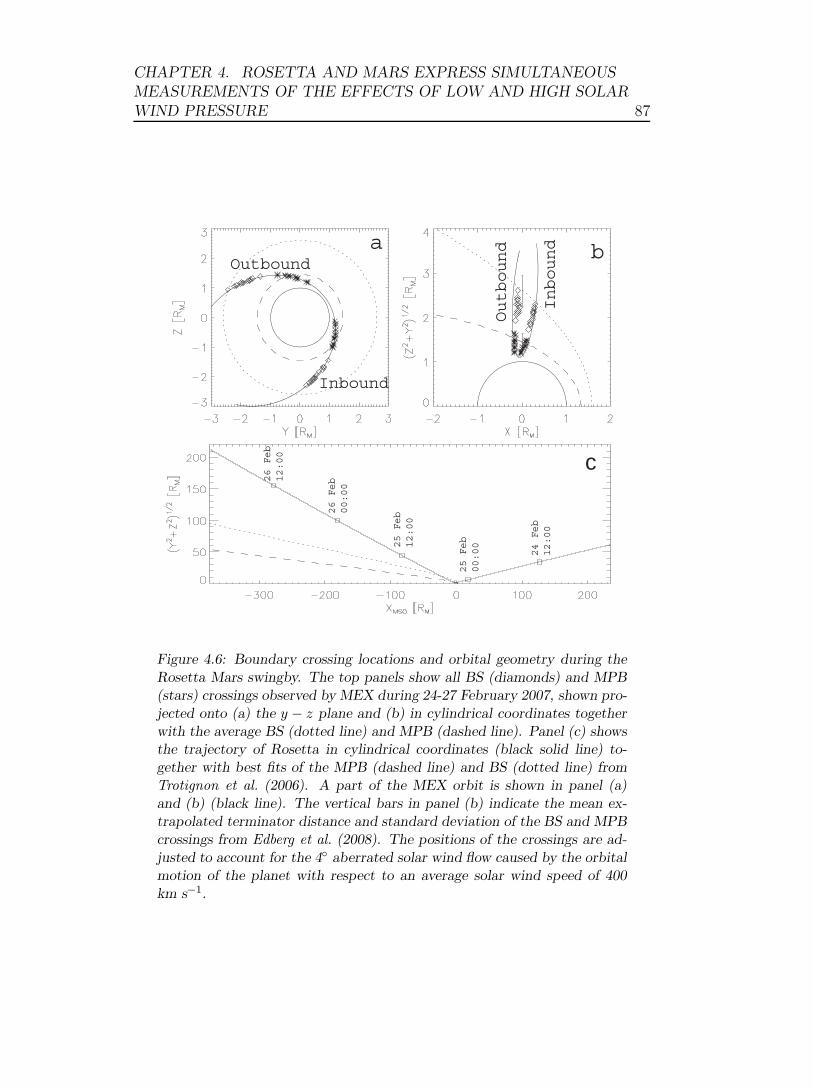
CHAPTER 4. ROSETTA AND MARS EXPRESS SIMULTANEOUSMEASUREMENTS OF THE EFFECTS OF LOW AND HIGH SOLARWIND PRESSURE 87
24 Feb
12:00
26 Feb
00:00
25 Feb
00:00
26 Feb
12:00
25 Feb
12:00
c
a b
Inbound
Outbound
Inbound
Outbound
Figure 4.6: Boundary crossing locations and orbital geometry during theRosetta Mars swingby. The top panels show all BS (diamonds) and MPB(stars) crossings observed by MEX during 24-27 February 2007, shown pro-jected onto (a) the y − z plane and (b) in cylindrical coordinates togetherwith the average BS (dotted line) and MPB (dashed line). Panel (c) showsthe trajectory of Rosetta in cylindrical coordinates (black solid line) to-gether with best fits of the MPB (dashed line) and BS (dotted line) fromTrotignon et al. (2006). A part of the MEX orbit is shown in panel (a)and (b) (black line). The vertical bars in panel (b) indicate the mean ex-trapolated terminator distance and standard deviation of the BS and MPBcrossings from Edberg et al. (2008). The positions of the crossings are ad-justed to account for the 4◦ aberrated solar wind flow caused by the orbitalmotion of the planet with respect to an average solar wind speed of 400km s−1.
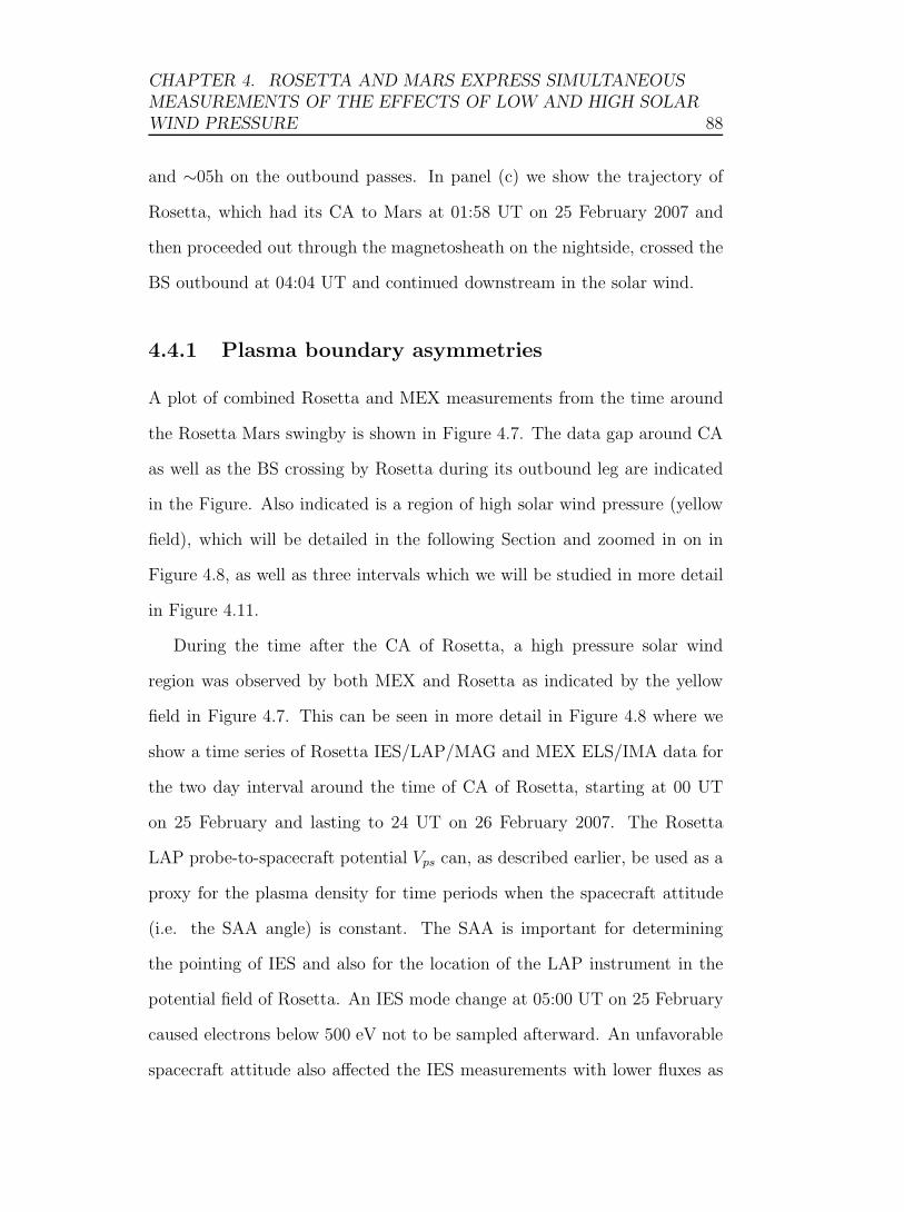
CHAPTER 4. ROSETTA AND MARS EXPRESS SIMULTANEOUSMEASUREMENTS OF THE EFFECTS OF LOW AND HIGH SOLARWIND PRESSURE 88
and ∼05h on the outbound passes. In panel (c) we show the trajectory of
Rosetta, which had its CA to Mars at 01:58 UT on 25 February 2007 and
then proceeded out through the magnetosheath on the nightside, crossed the
BS outbound at 04:04 UT and continued downstream in the solar wind.
4.4.1 Plasma boundary asymmetries
A plot of combined Rosetta and MEX measurements from the time around
the Rosetta Mars swingby is shown in Figure 4.7. The data gap around CA
as well as the BS crossing by Rosetta during its outbound leg are indicated
in the Figure. Also indicated is a region of high solar wind pressure (yellow
field), which will be detailed in the following Section and zoomed in on in
Figure 4.8, as well as three intervals which we will be studied in more detail
in Figure 4.11.
During the time after the CA of Rosetta, a high pressure solar wind
region was observed by both MEX and Rosetta as indicated by the yellow
field in Figure 4.7. This can be seen in more detail in Figure 4.8 where we
show a time series of Rosetta IES/LAP/MAG and MEX ELS/IMA data for
the two day interval around the time of CA of Rosetta, starting at 00 UT
on 25 February and lasting to 24 UT on 26 February 2007. The Rosetta
LAP probe-to-spacecraft potential Vps can, as described earlier, be used as a
proxy for the plasma density for time periods when the spacecraft attitude
(i.e. the SAA angle) is constant. The SAA is important for determining
the pointing of IES and also for the location of the LAP instrument in the
potential field of Rosetta. An IES mode change at 05:00 UT on 25 February
caused electrons below 500 eV not to be sampled afterward. An unfavorable
spacecraft attitude also affected the IES measurements with lower fluxes as
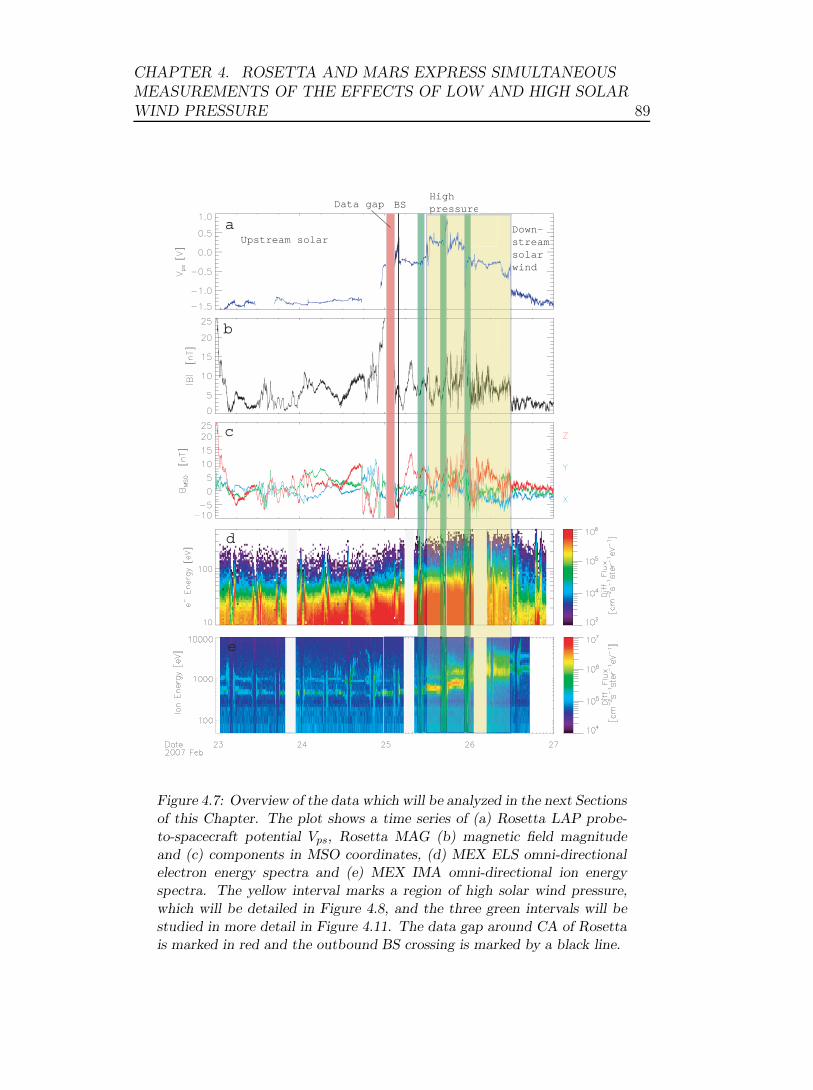
CHAPTER 4. ROSETTA AND MARS EXPRESS SIMULTANEOUSMEASUREMENTS OF THE EFFECTS OF LOW AND HIGH SOLARWIND PRESSURE 89
High pressureData gap BS
Upstream solar Down-streamsolar wind
a
b
c
d
e
Figure 4.7: Overview of the data which will be analyzed in the next Sectionsof this Chapter. The plot shows a time series of (a) Rosetta LAP probe-to-spacecraft potential Vps, Rosetta MAG (b) magnetic field magnitudeand (c) components in MSO coordinates, (d) MEX ELS omni-directionalelectron energy spectra and (e) MEX IMA omni-directional ion energyspectra. The yellow interval marks a region of high solar wind pressure,which will be detailed in Figure 4.8, and the three green intervals will bestudied in more detail in Figure 4.11. The data gap around CA of Rosettais marked in red and the outbound BS crossing is marked by a black line.
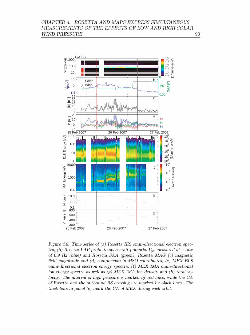
CHAPTER 4. ROSETTA AND MARS EXPRESS SIMULTANEOUSMEASUREMENTS OF THE EFFECTS OF LOW AND HIGH SOLARWIND PRESSURE 90
-100
-50
0
102103104105106107
05
10152025
|B| [
nT]
25 Feb 2007 26 Feb 2007 27 Feb 2007 -10
0
1020
B [n
T]
1
10
100
1000
ELS
Ene
rgy
[eV
]
103
104
105
106
[1/c
m -
s-sr
-eV
]
25 Feb 2007 27 Feb 2007
100
1000
10000
IMA
Ene
rgy
[eV
]
26 Feb 2007
104
105
106
[1/c
m -
s-sr
-eV
]
BS
Solar Wind
a
e
d
c
b
C/A
0.1
1.0
10.0
N [c
m
]-3
400
500600
V [k
m s
]
-1
300
f
g
10
100
1000
h
Ene
rgy
[eV
/q]
107
107
108
SA
A [
]0
-1. 5
0
1. 5
V ps [
V ]
BxByBz
22
[1/c
m -
s-sr
-eV
]2
Figure 4.8: Time series of (a) Rosetta IES omni-directional electron spec-tra, (b) Rosetta LAP probe-to-spacecraft potential Vps measured at a rateof 0.9 Hz (blue) and Rosetta SAA (green), Rosetta MAG (c) magneticfield magnitude and (d) components in MSO coordinates, (e) MEX ELSomni-directional electron energy spectra, (f) MEX IMA omni-directionalion energy spectra as well as (g) MEX IMA ion density and (h) total ve-locity. The interval of high pressure is marked by red lines, while the CAof Rosetta and the outbound BS crossing are marked by black lines. Thethick bars in panel (e) mark the CA of MEX during each orbit.
CHAPTER 4. ROSETTA AND MARS EXPRESS SIMULTANEOUSMEASUREMENTS OF THE EFFECTS OF LOW AND HIGH SOLARWIND PRESSURE 91
a result.
In Figure 4.8, at 11:49 UT on 25 February 2007 as indicated by the left
red vertical line, IMA onboard MEX observed a sudden solar wind density
increase from ∼1 cm−3 to a maximum of ∼10 cm−3. The MEX ELS instru-
ment also observed an increase in electron fluxes at the same time. This was
followed by a gradual increase in velocity from ∼350 km s−1 to a maximum
of ∼500 km s−1. For details regarding the moment calculation from IMA, see
Section 2.4 and Franz et al. (2006a). At 12:02 UT on 25 February 2007 the
IES, LAP and MAG on Rosetta observed an increase in electron flux in the
energy range 60−100 eV, a sharp increase in Vps, and an increase in magnetic
field variability, respectively. Rosetta was downstream of Mars at a distance
of 83 RM at this time. The spatial difference between where Rosetta starts
to observe the high pressure solar wind and where MEX observes it divided
by the difference in arrival times at the two spacecraft gives a velocity in the
MSO −x-direction of ∼360 km s−1 (83 RM divided by 13 min).
The density increase observed by MEX lasted until 11:22 UT on 26 Febru-
ary 2007, indicated by the right red vertical line, while the higher velocity
lasted longer, at least until a data gap started on 28 February 2007. At
Rosetta, Vps dropped suddenly (corresponding to a decrease in plasma den-
sity) at the same time as the magnetic field variability signatures stopped
and the electron fluxes decreased at 11:53 UT on 26 February 2007 at a
distance of 277 RM downstream of Mars. The difference in time between
these signatures in the data of the two spacecraft give a velocity in the MSO
−x-direction of ∼510 km s−1. The solar wind velocity measured by MEX
IMA agrees very well with the velocities derived from arrival times of similar
features at the two spacecraft (∼350 km s−1 compared to ∼360 km s−1 and
CHAPTER 4. ROSETTA AND MARS EXPRESS SIMULTANEOUSMEASUREMENTS OF THE EFFECTS OF LOW AND HIGH SOLARWIND PRESSURE 92
∼510 km s−1 compared to ∼500 km s−1). The velocity does not change across
the boundaries between regions of high and low pressure regions, as would
be expected from interplanetary shocks or corotating interaction regions, and
they rather resemble convected structures propagating outward in the solar
system. This observed high pressure solar wind region and its effect on the
Martian plasma environment is the topic for the rest of this Chapter.
To illustrate how the BS and MPB respond to the high pressure solar
wind region, we plot their altitudes as a time series together with the MEX
and Rosetta measurements in Figure 4.9. The time series shows four days of
combined Rosetta and MEX measurements starting at 00 UT on 24 February
2007. In panel (a) we show solar wind dynamic pressure derived from MEX
IMA and in panel (b) the Alfvenic Mach number MA based on a combination
of the magnetic field strength from Rosetta MAG, time-shifted to the time
frame of MEX assuming a constant solar wind velocity of 350 km s−1, and
the solar wind plasma density from MEX IMA. Panel (c) shows the angle
θBn between the IMF, as measured by Rosetta and time-shifted to the time
frame of MEX, and the local normal to the BS, for each inbound (squares)
and outbound (triangles) BS crossing by MEX. The local normal to the
BS was calculated from the statistical best fit shape of the BS from Edberg
et al. (2008) at the point closest to the observed BS crossing. Inbound and
outbound crossing data are displayed as squares and triangles, respectively,
throughout the Chapter. Panel (d) shows the distance of each BS crossing
from the center of the planet, for inbound and outbound crossings separately
and panel (e) shows the distance of the MPB crossings.
The inbound crossings occur at lower solar SZA than the outbound ones
and should therefore be at lower distances but this is evidently not always
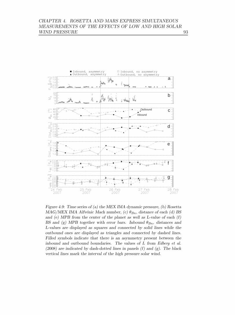
CHAPTER 4. ROSETTA AND MARS EXPRESS SIMULTANEOUSMEASUREMENTS OF THE EFFECTS OF LOW AND HIGH SOLARWIND PRESSURE 93
a
e
d
c
b
Inbound
Outbound
f
g
Inbound, no asymmetryOutbound, no asymmetry
Inbound, asymmetryOutbound, asymmetry
Figure 4.9: Time series of (a) the MEX IMA dynamic pressure, (b) RosettaMAG/MEX IMA Alfvenic Mach number, (c) θBn, distance of each (d) BSand (e) MPB from the center of the planet as well as L-value of each (f)BS and (g) MPB together with error bars. Inbound θBn, distances andL-values are displayed as squares and connected by solid lines while theoutbound ones are displayed as triangles and connected by dashed lines.Filled symbols indicate that there is an asymmetry present between theinbound and outbound boundaries. The values of L from Edberg et al.(2008) are indicated by dash-dotted lines in panels (f) and (g). The blackvertical lines mark the interval of the high pressure solar wind.
CHAPTER 4. ROSETTA AND MARS EXPRESS SIMULTANEOUSMEASUREMENTS OF THE EFFECTS OF LOW AND HIGH SOLARWIND PRESSURE 94
the case. The inbound crossings are sometimes at larger distances than
the outbound crossing during the same orbit. Hence the boundaries are
asymmetric in their shapes. In order to properly compare the distances of
inbound crossings with the distance of the outbound crossings, which occur
at different SZAs, we need a measure of their distances which is independent
of the SZA at which they occur. Panel (f) therefore shows the value of the
semi-latus rectum L from fits of conic sections to each single BS crossing.
The fits are done in the same way as described in Crider et al. (2002), where
the values of ε and X0 (from (Edberg et al., 2008)) are fixed, and only L is
varied. L is hence a linear measure of the distance of a crossing for which the
SZA dependence has been removed. Panel (g) shows the same as panel (f)
but for the MPB instead of the BS. Due to the orbit configuration, upstream
waves and also the movement of the boundaries, the two boundaries do not
always appear as sharp boundaries but are at times more or less smeared out
in a time series. This gives an uncertainty to where the boundary crossings
actually occur. The uncertainty bars in panel (f) and (g) represent where
the spacecraft is well within/without the BS and the MPB, as seen in a time
series of data, and hence are estimates of the thicknesses of the boundaries,
or their variability in position during each crossing.
The position of each crossing is adjusted to account for the 4◦ aberration
caused by the planets orbital velocity. The average values of L for the BS
and MPB from Edberg et al. (2008) are shown for reference purposes by the
horizontal dash-dotted lines in panel (d) and (e). The inbound and outbound
crossings of both the BS and the MPB are at approximately similar altitudes
(L-values) up until the high pressure solar wind appears. They are also closer
than average to the planet in the time interval preceding the high pressure
CHAPTER 4. ROSETTA AND MARS EXPRESS SIMULTANEOUSMEASUREMENTS OF THE EFFECTS OF LOW AND HIGH SOLARWIND PRESSURE 95
solar wind. During and after the high pressure solar wind the altitude of the
inbound and outbound crossings deviate significantly from each other, by up
to 0.7 RM for the BS and 0.4 RM for the MPB and hence properly indicate
that both boundaries have become asymmetric. The inbound boundaries
move outward first and the outbound boundaries follow later on.
The asymmetry of the MPB starts during the same orbit as the high pres-
sure solar wind feature is observed and the BS asymmetry starts during the
following orbit. The shape asymmetry lasts until about two orbits after the
solar wind feature has passed. As reported by Perez-de-Tejada et al. (2009),
the exosphere of Mars, as seen in X-ray images from the XMM/Newton
satellite, is also very asymmetric during this interval. The X-ray emissions
from the exosphere are more intense over the poles and also indicate that
the exosphere over the poles is tilted in an anti-sunward direction. Note also
that there is a short-lived BS asymmetry during the last orbit on 24 Febru-
ary 2007. Throughout this Chapter, filled symbols indicate that there is an
asymmetry present between the inbound and outbound crossings.
4.4.2 Cause of the asymmetries
Factors that could be responsible for the asymmetry include whether the
boundaries are quasi-perpendicular or quasi-parallel, the direction of the solar
wind convective electric field E = −v × B and the crustal magnetic fields.
1. The quasi-parallel (quasi-perpendicular) effect could cause increased
(decreased) upstream wave activity which increases (decreases) the ap-
parent thickness of the boundaries. This has already been accounted
for to some extent by including the error bars in Figure 4.9 but it is
possible that the boundaries also move outward or inward as a whole

CHAPTER 4. ROSETTA AND MARS EXPRESS SIMULTANEOUSMEASUREMENTS OF THE EFFECTS OF LOW AND HIGH SOLARWIND PRESSURE 96
due to this.
2. The convective electric fields determines in which way the ions move.
On one side of the planet they will move into the planet and on the
opposite side they will move out into the solar wind and cause increased
massloading which could cause the boundaries to move outward due to
the increased plasma pressure.
3. The crustal magnetic fields provide additional magnetic pressure which
disturbs the pressure balance across the boundaries and would cause
the boundaries to move outward. Since the crustal magnetic fields
are strongest and most frequently observed at southern latitudes the
boundaries should be at higher altitudes over the southern hemisphere.
In Figure 4.10 we show the results of tests of the above factors that could
possibly cause the asymmetry. In panel (a) and (b) we show the value of
the semi-latus rectum L from fits to each observed BS and MPB crossing,
respectively, as a function of θBn together with linear least-square fits to the
inbound (solid line) and outbound (dashed line) crossings. The difference in
mean value of the semi-latus rectum of all quasi-parallel (θBn < 45◦) and all
quasi-perpendicular (θBn > 45◦) BS crossings (1.77 and 1.62, respectively) is
statistically significant according to a Student’s t-test at a 90% confidence
level. However, if a Student’s t-test is done separately for inbound and
outbound BS crossings, then only the inbound crossings show a significant
difference in mean values of L at a confidence level of 90%. An equally
significant difference between mean values of the semi-latus rectum is not
found for the MPB. There is a trend of a closer in boundary for higher θBn
in panel (a) and panel (b), but only for the crossings that occur when the

CHAPTER 4. ROSETTA AND MARS EXPRESS SIMULTANEOUSMEASUREMENTS OF THE EFFECTS OF LOW AND HIGH SOLARWIND PRESSURE 97
ba
c d
fe
Inbound, no asymmetryOutbound, no asymmetryInbound, asymmetryOutbound, asymmetry
Figure 4.10: The distance displayed in terms of L-value (see text for expla-nation) of (a) the BS and (b) the MPB crossings as a function of θBn withlinear fits to the inbound (solid) and the outbound (open) crossings. Theposition (c) of all BS and (d) MPB crossings rotated into a frame where Y
′
is aligned with the IMF and Z′with the convection electric field. Average
distances are shown for inbound (solid line) and outbound (dashed line)crossings in the +E and −E hemispheres in panels (c) and (d). The posi-tion (e) of all BS and (f) MPB crossings projected onto a map of the crustalmagnetic field strength (the position data being coloured red in order tomake them more visible).

CHAPTER 4. ROSETTA AND MARS EXPRESS SIMULTANEOUSMEASUREMENTS OF THE EFFECTS OF LOW AND HIGH SOLARWIND PRESSURE 98
boundary is asymmetric and not for the other crossings. This rather tells us
that the crossings that occur during the asymmetric boundary interval and
are on the inbound side also happen to be quasi-parallel and vice versa but
not that it is the θBn angle that determines the altitude of the boundaries.
In panel (c) and (d) of Figure 4.10 we show all BS and MPB crossings
rotated into a reference frame where Y ′ is aligned with the instantaneous
IMF direction, as measured by Rosetta MAG, and Z ′ with the convection
electric field direction, in order to determine the effect of the convection
electric field. Average distances are displayed for inbound (dashed line) and
outbound (solid line) crossings in both the +E-hemisphere, where the electric
field is directed locally upward, and in the −E hemisphere, where the electric
field is directed locally downward. If asymmetric massloading occurred and
was the main factor which controlled the location of the boundaries, then the
boundaries in the +E-hemisphere, where the ions move out into the solar
wind, would be at higher altitudes than the ones in the −E-hemisphere,
where the ions move toward the planet. However, no such trend is observed
for either the BS or the MPB, neither during high nor low pressure periods.
We do, however, observe that in the −E-hemisphere the inbound cross-
ings, in the southern/dusk hemisphere, are farther out than the outbound
crossings. The difference is statistically significant according to Student’s
t-test at a 95% confidence level for the BS and at a 90% confidence level
for the MPB. This asymmetry is not visible for the +E-hemisphere. Since
the evolution of the IMF orientation with distance is unknown, there could
be a difference in IMF orientation between the location where Rosetta mea-
sures the magnetic field and the location where MEX measures the plasma
boundaries.
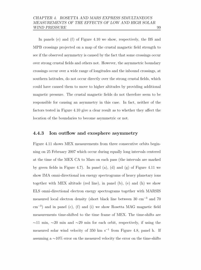
CHAPTER 4. ROSETTA AND MARS EXPRESS SIMULTANEOUSMEASUREMENTS OF THE EFFECTS OF LOW AND HIGH SOLARWIND PRESSURE 99
In panels (e) and (f) of Figure 4.10 we show, respectively, the BS and
MPB crossings projected on a map of the crustal magnetic field strength to
see if the observed asymmetry is caused by the fact that some crossings occur
over strong crustal fields and others not. However, the asymmetric boundary
crossings occur over a wide range of longitudes and the inbound crossings, at
southern latitudes, do not occur directly over the strong crustal fields, which
could have caused them to move to higher altitudes by providing additional
magnetic pressure. The crustal magnetic fields do not therefore seem to be
responsible for causing an asymmetry in this case. In fact, neither of the
factors tested in Figure 4.10 give a clear result as to whether they affect the
location of the boundaries to become asymmetric or not.
4.4.3 Ion outflow and exosphere asymmetry
Figure 4.11 shows MEX measurements from three consecutive orbits begin-
ning on 25 February 2007 which occur during equally long intervals centered
at the time of the MEX CA to Mars on each pass (the intervals are marked
by green fields in Figure 4.7). In panel (a), (d) and (g) of Figure 4.11 we
show IMA omni-directional ion energy spectrograms of heavy planetary ions
together with MEX altitude (red line), in panel (b), (e) and (h) we show
ELS omni-directional electron energy spectrograms together with MARSIS
measured local electron density (short black line between 30 cm−3 and 70
cm−3) and in panel (c), (f) and (i) we show Rosetta MAG magnetic field
measurements time-shifted to the time frame of MEX. The time-shifts are
∼11 min, ∼20 min and ∼29 min for each orbit, respectively, if using the
measured solar wind velocity of 350 km s−1 from Figure 4.8, panel h. If
assuming a ∼10% error on the measured velocity the error on the time-shifts

CHAPTER 4. ROSETTA AND MARS EXPRESS SIMULTANEOUSMEASUREMENTS OF THE EFFECTS OF LOW AND HIGH SOLARWIND PRESSURE 100
are ±1 − 2min. There are only MARSIS density measurements during ∼5
min on the outbound part of the first orbit, ∼5 min during both the inbound
and the outbound part of the second orbit and only ∼5 min during the in-
bound part of the third orbit, but these are still important since they provide
a measure of the local plasma density. IMA and ELS can also provide values
of the density but do not always measure the full density, especially not the
colder population, which MARSIS does.
Panels (d) and (e) of Figure 4.11 show the same data as presented by
Perez-de-Tejada et al. (2009) (their Figure 2). From 17:10 until 17:40 UT in
panel (d) a distinct population of heavy ions (mainly CO+2 , O+
2 and O+) are
seen in the energy range 100 eV - 10 keV, around the time of the outbound
MPB crossing, which are interpreted as being heavy planetary ions escaping
from the planet. These ions show a clear trend of increasing in energy as
MEX measures them at higher and higher altitudes and they reach velocities
far higher than the required escape velocity (Perez-de-Tejada et al., 2009).
Not reported by Perez-de-Tejada et al. (2009) is that such escaping plan-
etary ions are also visible on the following orbit, in almost exactly the same
location but with an order of magnitude less intensity. These are seen in
panel (g) from 23:55 UT on 25 February until 00:15 UT on 26 February,
again as a distinct population which gain in energy, from 100 eV up to 1
keV, while MEX measures them at higher altitude. The population of escap-
ing ions during this orbit is now harder to distinguish from the background
measurements but still visible.
It is during these two orbits, when escaping planetary ions are observed,
that the solar wind pressure increases to high values of ∼1.0-1.5 nPa as
can be seen in panel (a) of Figure 4.9. The magnetic field measurements
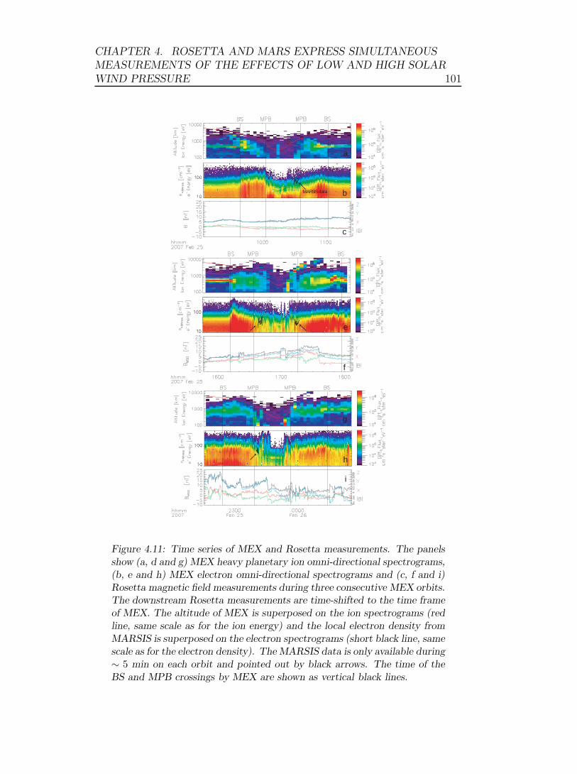
CHAPTER 4. ROSETTA AND MARS EXPRESS SIMULTANEOUSMEASUREMENTS OF THE EFFECTS OF LOW AND HIGH SOLARWIND PRESSURE 101
a
b
f
e
d
c
g
h
i
MARSIS data
Figure 4.11: Time series of MEX and Rosetta measurements. The panelsshow (a, d and g) MEX heavy planetary ion omni-directional spectrograms,(b, e and h) MEX electron omni-directional spectrograms and (c, f and i)Rosetta magnetic field measurements during three consecutive MEX orbits.The downstream Rosetta measurements are time-shifted to the time frameof MEX. The altitude of MEX is superposed on the ion spectrograms (redline, same scale as for the ion energy) and the local electron density fromMARSIS is superposed on the electron spectrograms (short black line, samescale as for the electron density). The MARSIS data is only available during∼ 5 min on each orbit and pointed out by black arrows. The time of theBS and MPB crossings by MEX are shown as vertical black lines.

CHAPTER 4. ROSETTA AND MARS EXPRESS SIMULTANEOUSMEASUREMENTS OF THE EFFECTS OF LOW AND HIGH SOLARWIND PRESSURE 102
show that the IMF was mainly northward during these orbits which gives
a convective electric field direction mainly in the MSO −y-direction. The
convective electric field is in the same direction, roughly, as MEX moves in
when the escaping planetary ions are observed (see MEX trajectory in Figure
4.6, panel (a)). As the ions are observed to gain in energy we can conclude
that they are accelerated by the convective electric field. At the same time
as the magnetic field changes its orientation at 17:40 UT (Fig. 4.11, panel
(d)) the escaping ions cease being observed in the ion spectrogram. Perez-
de-Tejada et al. (2009) also noted this sharp drop but suggested that it
was caused by momentum transport between the planetary ions and the
solar wind ions. But with the magnetic field measurements from Rosetta we
now suggest that the sharp drop is caused by a change of direction of the
convection electric field, rotating from −y to +z, such that the outflowing
ions start to move northward while MEX moves farther westward and ceases
to observe the outflowing ions. During the second orbit when these ions
are observed, the IMF direction is still mainly northward but more variable
which could explain why the measured flux rates are lower than during the
previous orbit.
The local electron densities measured by MARSIS just inside the MPB on
the first orbit in Figure 4.11, panel (b), are ∼70 cm−3. During the following
orbit, in panel (e), at the same altitudes on the outbound pass as in the
previous orbit, the density had dropped to values of ∼30 cm−3. Also during
the inbound pass of the second orbit the densities, at approximately the same
altitudes, vary around 30 cm−3. During the third orbit, on the inbound leg in
panel (h), the average density had increased to around 70 cm−3 again. These
limited measurements from MARSIS indicate, in the same way as shown by

CHAPTER 4. ROSETTA AND MARS EXPRESS SIMULTANEOUSMEASUREMENTS OF THE EFFECTS OF LOW AND HIGH SOLARWIND PRESSURE 103
Dubinin et al. (2009) but for a different interval, that the ionospheric densities
inside the MPB decreased when the high pressure solar wind impacted Mars
and therefore the ionosphere was being scavenged as a result.
As shown in Figure 4.9, the boundaries start to become asymmetric during
this interval. This can be clearly seen in Figure 4.11 as well. The inbound BS
moves to increasingly higher altitudes during the three orbits shown, from
an L-value of 1.51 RM to 1.78 RM to 1.90 RM , even though the dynamic
pressure increases and should push the boundary closer in. The inbound
MPB follows the same trend roughly, or at least within the error bars, and
moves from an L-value of 0.70 RM to 0.98 RM to 0.92 RM . The outbound
MPB does, however, move inward during these three orbits, from 0.82 RM
to 0.76 RM to 0.65 RM . The outbound BS first moves outward, from 1.53
RM to 1.73 RM like the inbound BS, but only to move inward again during
the third orbit to 1.46 RM , when the solar wind dynamic pressure decreases.
These data clearly show that the dynamic pressure is not always the only
important factor in determining the location of the plasma boundaries.
4.5 Boundary asymmetry linked to the iono-
spheric outflow
Below, we try to explain the observations of the asymmetric boundaries by
discussing the various factors involved. According to Figure 4.10, panel (a)
and (b), the BS and MPB asymmetries are generally only present when the
inbound crossings are quasi-parallel and the outbound crossings are quasi-
perpendicular. We cannot, however, conclude that the effect of the difference
between quasi-parallel and quasi-perpendicular crossings is the only reason

CHAPTER 4. ROSETTA AND MARS EXPRESS SIMULTANEOUSMEASUREMENTS OF THE EFFECTS OF LOW AND HIGH SOLARWIND PRESSURE 104
for the asymmetry. We can only conclude that when there is an asymme-
try present, the inbound and outbound crossings have significantly different
values of θBn. Other factors could still be important.
In Figure 4.10, panel (c) and (d), we have shown that asymmetric mass-
loading is not the single responsible factor for causing the boundary asym-
metries. The boundary crossings that occur in the +E-hemisphere are not at
higher altitudes than the crossings observed in the −E-hemisphere, on aver-
age. We do, however, note that the boundaries in the southern and northern
hemispheres of Mars react differently to different directions of the convec-
tion electric field, possibly due to the presence of the southern crustal fields
or, alternatively, due to whether the boundaries are quasi-perpendicular or
quasi-parallel.
In Figure 4.10, panels (e) and (f), we do not find a direct correlation be-
tween the crustal field strength at the exact position of the BS/MPB crossings
and the boundary distances. However, it is in the southern hemisphere that
the boundaries are at higher altitudes but since the MEX crossings occur at
a range of longitudes it would imply a global influence of the crustal fields,
if they are indeed responsible.
The Alfvenic Mach number and dynamic pressure variation do not di-
rectly explain the asymmetry, either. These quantities could possibly vary
in resonance with the boundary sampling rate, which is unlikely and indeed
not the case here since the solar wind parameters do not vary with the same
frequency as the boundaries move up and down. A comparison between the
altitudes of all crossings and the solar wind dynamic pressure and Alfvenic
Mach number reveals no obvious trend for the set of crossings in this interval.
Since none of the above factors have been clearly shown to be the single
CHAPTER 4. ROSETTA AND MARS EXPRESS SIMULTANEOUSMEASUREMENTS OF THE EFFECTS OF LOW AND HIGH SOLARWIND PRESSURE 105
main factor that causes the asymmetry we suggest that the high pressure so-
lar wind and the ion outflow are also connected to the observed asymmetries.
The ion outflow can disturb the normal balance between factors that would
be expected to control the location of the boundaries, i.e. the solar wind dy-
namic pressure, the IMF direction, the plasma pressure, magnetic pressure
and the crustal fields and we can therefore only provide a suggestion for a
possible explanation to the observations. The MPB and BS in the southern
hemisphere, quite counter-intuitively, move outward when the high pressure
solar wind reaches Mars as can be seen in Figure 4.11 and which we try to
illustrate by the sketch in Figure 4.12. We interpret the outward moving of
the boundaries as the plasma pressure and/or magnetic pressure inside the
MPB and BS are significantly increasing during the high pressure solar wind
and more so than the solar wind dynamic pressure, resulting in an outward
motion of the boundaries. The pressure on the inside could increase due to an
increased massloading over a longer time period on that side of the planet in
combination with increased massloading over the crustal fields on the other
side, and possibly as an effect of plasma heating through reconnection events
when the varying IMF direction reaches the crustal fields.
The convective electric field is directed toward the planet in the south-
ern/dusk hemisphere and the ions consequently move in that direction. In
the opposite northern/dawn hemisphere the convective electric field is di-
rected away from the planet and the ions can escape the planet and the
plasma pressure on the inside of the MPB and BS decreases, which leads to
an eventual inward motion of the plasma boundaries. The BS during the
outbound part of the orbit immediately after the high pressure region has
reached Mars does, however, initially move outward, which could be an effect
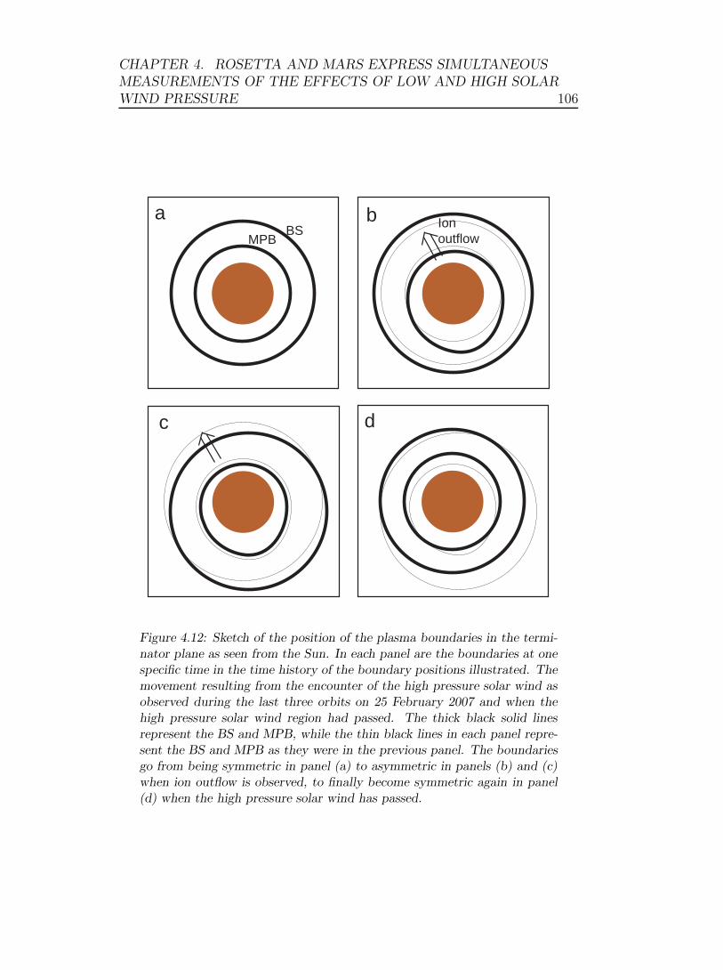
CHAPTER 4. ROSETTA AND MARS EXPRESS SIMULTANEOUSMEASUREMENTS OF THE EFFECTS OF LOW AND HIGH SOLARWIND PRESSURE 106
BSa b
c
MPBIonoutflow
d
Figure 4.12: Sketch of the position of the plasma boundaries in the termi-nator plane as seen from the Sun. In each panel are the boundaries at onespecific time in the time history of the boundary positions illustrated. Themovement resulting from the encounter of the high pressure solar wind asobserved during the last three orbits on 25 February 2007 and when thehigh pressure solar wind region had passed. The thick black solid linesrepresent the BS and MPB, while the thin black lines in each panel repre-sent the BS and MPB as they were in the previous panel. The boundariesgo from being symmetric in panel (a) to asymmetric in panels (b) and (c)when ion outflow is observed, to finally become symmetric again in panel(d) when the high pressure solar wind has passed.
CHAPTER 4. ROSETTA AND MARS EXPRESS SIMULTANEOUSMEASUREMENTS OF THE EFFECTS OF LOW AND HIGH SOLARWIND PRESSURE 107
of massloading of the solar wind by the outflowing planetary ions. The BS
therefore first moves outward but after the ionosphere has eroded during the
time of at least one orbit the pressure on the inside of the BS has decreased
so much that the boundaries then can move inward on that side of the planet
and the boundary become asymmetric. When the high pressure region has
passed the boundaries become symmetric again.
4.6 Summary and conclusions
The Rosetta flyby adds to the growing number of spacecraft that have sam-
pled the Martian plasma environment. We have performed a rigorous analy-
sis of the simultaneous measurements performed by the Rosetta instruments
and the MEX measurements during the time of the Rosetta Mars flyby in
February 2007. First, we have analyzed the measurements around the time
of CA of Rosetta when both Rosetta and MEX sampled the plasma bound-
aries. Secondly, we have analyzed the measurements when Rosetta acted as
a solar wind monitor and MEX sampled the plasma boundaries alone.
When both spacecraft sampled the plasma environment simultaneously
we could perform the first near-simultaneous two-spacecraft study of the
shape and location of the BS, MPB and PEB. At this time, the solar wind
appeared to be quiet and slow and so the global plasma environment could be
assumed to be more or less steady. The shape of the plasma boundaries were,
for the first time, experimentally compared to previous models (Figure 4.5).
The far downstream triple BS crossings observed by Rosetta at approximately
04:04 UT are also the most distant BS crossings ever observed at Mars: at
∼18 RM behind the planet.
CHAPTER 4. ROSETTA AND MARS EXPRESS SIMULTANEOUSMEASUREMENTS OF THE EFFECTS OF LOW AND HIGH SOLARWIND PRESSURE 108
The BS is generally found to be located closer to the planet than average
compared to what models would suggest for all crossings in this time interval,
even though the upstream solar wind speed is low and the density and IMF
are moderate. For two of the BS crossings (the inbound Rosetta crossing
and the outbound MEX crossing), this can be explained by the fact that
they are observed over the northern hemisphere of Mars where the BS has
been observed to be closer to the planet. The inbound MEX BS crossing
is observed over the southern hemisphere and is the crossing observed the
farthest out. Another explanation could be that the thermal plasma pressure
in the magnetosheath is lower than average at this time, and the effective
solar wind obstacle thereby smaller, which puts the BS closer in than average.
The shape of the BS is still reasonably well represented by a conic section.
The MPB is observed very close to its average position and also seems to be
well represented by a conic section in its shape.
The PEB crossings observed seems to form the same shape as the MPB
on the dayside. However, the crossings of this boundary takes place very
distant in time and close in space which makes it hard to determine the
shape accurately and we have not put any focus on the shape of the PEB in
this Chapter.
When Rosetta acted as a solar wind monitor, both Rosetta and MEX
show measurements of a high pressure (dynamic, magnetic and thermal, as
can be inferred from Figure 4.8) solar wind region that passed by Mars during
a 24 hour interval. At the same time as the high pressure solar wind passed
by, the Martian plasma boundaries as well as the exosphere are found to
become asymmetric in shape. Also, an outflow of planetary ions was observed
over the northern polar region of Mars in the same interval. During 4-5
CHAPTER 4. ROSETTA AND MARS EXPRESS SIMULTANEOUSMEASUREMENTS OF THE EFFECTS OF LOW AND HIGH SOLARWIND PRESSURE 109
orbits following the impact of the high pressure solar wind region, the BS
and MPB as observed inbound by MEX, in the southern/dusk hemisphere,
were much farther out than the BS and MPB observed outbound, in the
northern/dawn hemisphere. As reported by Dubinin et al. (2009) and Nilsson
et al. (2009) the ion outflow from Mars increases during high pressure solar
wind and this has also been confirmed by models, see e.g. (Kaneda et al.,
2009). Planetary ion outflow was, in fact, also remotely observed to occur
during the time of the Rosetta swingby (Perez-de-Tejada et al., 2009). In
this Chapter, we have combined these results and further strengthened the
evidence that high pressure solar wind causes an increase of planetary ion
outflow from Mars. The high pressure solar wind, observed by MAG and LAP
on Rosetta and IMA and ELS on MEX, penetrated down to the ionosphere
and eroded it, as observed by MARSIS on MEX, and planetary plasma was
observed to escape from the planet, as observed by IMA on MEX. The solar
wind plasma could also penetrate down to the ionosphere more easily during
this interval since both the BS and MPB were generally located closer in
than average on the orbits preceding the high pressure solar wind. The
escaping ions, as observed by MEX, gained in energy in the direction, as
indicated by Rosetta MAG measurements, of the convective electric field.
The exosphere was extended over both poles and the ion outflow was observed
over the northern hemisphere (Perez-de-Tejada et al., 2009). There have
been a number studies modelling the outflow of planetary ions from Mars,
see e.g. Boßwetter et al. (2004); Modolo et al. (2006); Kallio et al. (2008),
which also show that an increased solar wind dynamic pressure compresses
the plasma environment to some degree. However, little modelling has been
done in terms of asymmetric outflow and how that would cause the plasma
CHAPTER 4. ROSETTA AND MARS EXPRESS SIMULTANEOUSMEASUREMENTS OF THE EFFECTS OF LOW AND HIGH SOLARWIND PRESSURE 110
boundaries to become asymmetric. Kallio and Janhunen (2002) did however
show that both the MPB and the outflow is asymmetric and takes place
mainly in one hemisphere, which was determined by the direction of the
convective electric field.
In summary, the boundaries are well represented by conic sections, as
determined by near-simultaneous measurements. We conclude that the high
pressure solar wind enables the increased erosion of the ionosphere of Mars
at this time. At the same time as the high pressure solar wind impacts on
Mars are the boundaries observed to become asymmetric in their shapes. We
suggest that since no clear factor has emerged that causes the asymmetry, it
is possible that the observed outflow also disturbs the equilibrium pressure
balance and significantly influences the location and shape of the plasma
boundaries.

Chapter 5Mars Express and Mars Global
Surveyor measurements
In this Chapter we use MEX and MGS simultaneous and non-simultaneous
measurements to study the Martian plasma environment. In particular, we
derive quantitative expressions for the altitude of the terminator BS and
MPB as functions of solar wind dynamic pressure, crustal magnetic fields
and solar EUV flux. We also study the influence of the IMF direction. Some
of the material presented in this Chapter is included in Edberg et al. (2009b).
5.1 Introduction
MGS and MEX form a unique pair of spacecraft that have made simultane-
ous and continuous measurements of the Martian plasma environment. MGS
arrived at Mars in 1997 and performed measurements until late 2006, while
MEX arrived in late 2003 and is still gathering data as of 2009. Hence the two
spacecraft obtained almost three years of simultaneous measurements. There
have been many missions to Mars in the past equipped with plasma instru-
111
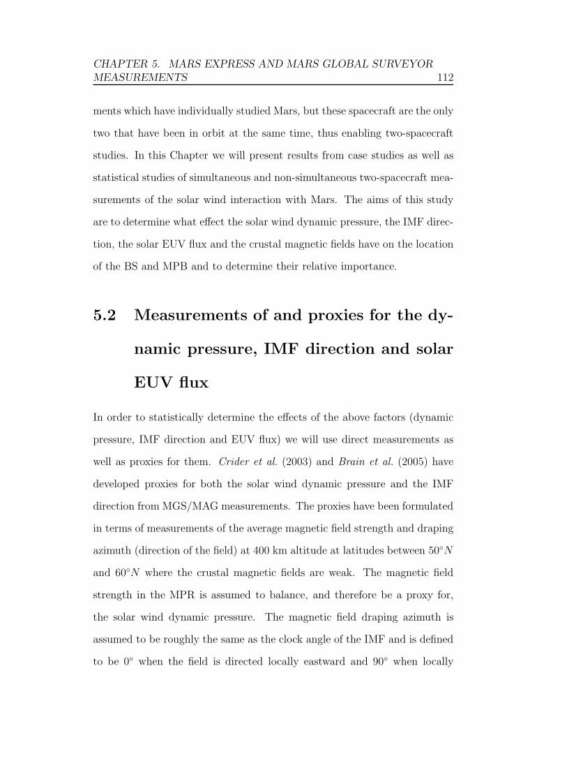
CHAPTER 5. MARS EXPRESS AND MARS GLOBAL SURVEYORMEASUREMENTS 112
ments which have individually studied Mars, but these spacecraft are the only
two that have been in orbit at the same time, thus enabling two-spacecraft
studies. In this Chapter we will present results from case studies as well as
statistical studies of simultaneous and non-simultaneous two-spacecraft mea-
surements of the solar wind interaction with Mars. The aims of this study
are to determine what effect the solar wind dynamic pressure, the IMF direc-
tion, the solar EUV flux and the crustal magnetic fields have on the location
of the BS and MPB and to determine their relative importance.
5.2 Measurements of and proxies for the dy-
namic pressure, IMF direction and solar
EUV flux
In order to statistically determine the effects of the above factors (dynamic
pressure, IMF direction and EUV flux) we will use direct measurements as
well as proxies for them. Crider et al. (2003) and Brain et al. (2005) have
developed proxies for both the solar wind dynamic pressure and the IMF
direction from MGS/MAG measurements. The proxies have been formulated
in terms of measurements of the average magnetic field strength and draping
azimuth (direction of the field) at 400 km altitude at latitudes between 50◦N
and 60◦N where the crustal magnetic fields are weak. The magnetic field
strength in the MPR is assumed to balance, and therefore be a proxy for,
the solar wind dynamic pressure. The magnetic field draping azimuth is
assumed to be roughly the same as the clock angle of the IMF and is defined
to be 0◦ when the field is directed locally eastward and 90◦ when locally

CHAPTER 5. MARS EXPRESS AND MARS GLOBAL SURVEYORMEASUREMENTS 113
northward. The pressure proxy is given by the magnetic field strength Bproxy
which can be converted to magnetic pressure PB =B2
proxy
2μ0.
A solar EUV flux proxy has also been developed and is determined from
the F10.7 radio flux at 2-200 nm measurements at Earth extrapolated to
Mars. The technique has been used by Mitchell et al. (2001) and here we use
the proxy developed in that study.
The solar wind (proton) velocity v and density n moments can be cal-
culated from MEX/IMA measurements outside of the BS which is a more
direct measurement of the solar wind dynamic pressure Pdyn = mpnv2, where
mp is the proton mass. Proton velocity and density moments are calculated
from the nominal proton line in the IMA spectrogram for energies above 1
keV, and below that energy from a signal caused by protons scattered inside
the IMA sensor. For details regarding the moment calculations, see Section
2.4 and Franz et al. (2006a). The pressure determined from MEX that we
will use in this Chapter is calculated as a mean over 10 min of measurements
exterior to a BS crossing.
The time resolution of both the MGS proxies are normally 2 hours (one
value per orbit) whereas the time resolution of the dynamic pressure mea-
sured by MEX is normally 2 samples per 6 hours (one value inbound and
one value outbound) and the time resolution of the EUV flux proxy is 1 to
2 hour.
In Figure 5.1 we show a comparison between the MGS proxy for the
solar wind dynamic pressure and the measured solar wind dynamic pressure
from MEX. In panel (a) the MGS pressure proxy values are interpolated
to the time of the MEX measured values and only data points during the
overlapping mission time are included. There is a visible linear trend in the
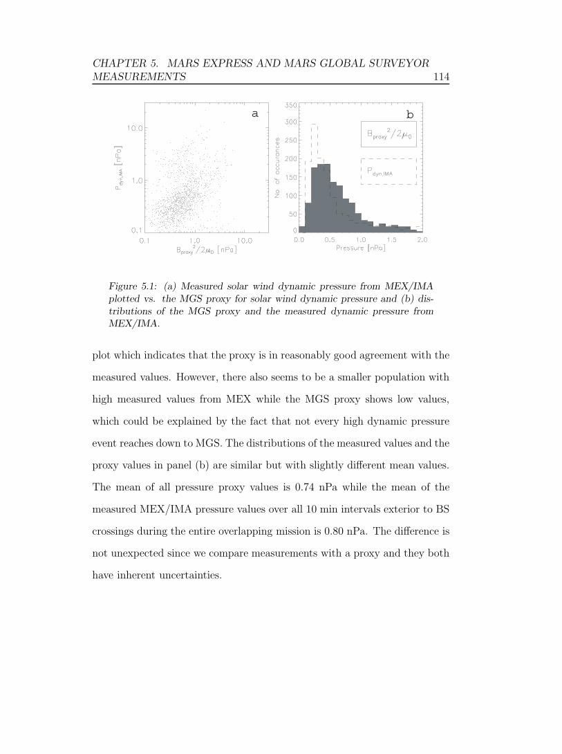
CHAPTER 5. MARS EXPRESS AND MARS GLOBAL SURVEYORMEASUREMENTS 114
a b
Figure 5.1: (a) Measured solar wind dynamic pressure from MEX/IMAplotted vs. the MGS proxy for solar wind dynamic pressure and (b) dis-tributions of the MGS proxy and the measured dynamic pressure fromMEX/IMA.
plot which indicates that the proxy is in reasonably good agreement with the
measured values. However, there also seems to be a smaller population with
high measured values from MEX while the MGS proxy shows low values,
which could be explained by the fact that not every high dynamic pressure
event reaches down to MGS. The distributions of the measured values and the
proxy values in panel (b) are similar but with slightly different mean values.
The mean of all pressure proxy values is 0.74 nPa while the mean of the
measured MEX/IMA pressure values over all 10 min intervals exterior to BS
crossings during the entire overlapping mission is 0.80 nPa. The difference is
not unexpected since we compare measurements with a proxy and they both
have inherent uncertainties.
CHAPTER 5. MARS EXPRESS AND MARS GLOBAL SURVEYORMEASUREMENTS 115
5.3 Mars Express and Mars Global Surveyor
observations
Since MEX is in a highly elliptical orbit with a low altitude periapsis it usu-
ally crosses both the MPB and the BS both inbound and outbound once
every orbit. The BS is, however, not always observed since the orbit of MEX
is precessing and therefore MEX stays inside the BS during the entire or-
bit in some seasons. The BS is observed inbound as a sudden increase in
fluxes of both electrons and ions in the ELS and IMA data sets. The MPB
is observed inbound as a sudden decrease of magnetosheath electron and ion
fluxes (examples of which will be presented in Figures 5.3-5.5 below). The
higher time resolution of ELS makes it easier to identify the exact location
of the boundaries from that data set. The variability of the boundaries in
combination with unfavorable orbit geometry makes it hard to identify the
exact boundary location for many of the orbits and many crossings are there-
fore excluded. However, we have analyzed the entire set of MEX/ELS and
MEX/IMA data from 2004 until 2009 and have identified 5014 MPB cross-
ings and 3277 BS crossings. The number of crossings during the overlapping
mission time between MGS and MEX (Feb 2004 - Nov 2006) decreases to
2500 and 1840, respectively, which is still twice as many as MGS observed
from 1997 until 1999 when MGS was in an elliptic orbit similar to the orbit
of MEX (Vignes et al., 2002; Trotignon et al., 2006; Edberg et al., 2008).
It should be noted that we can only get values of the measured solar wind
dynamic pressure when the BS is crossed, meaning that we do not know the
upstream pressure for all the 5014 MPB crossings.
During the overlapping mission time, MGS orbited Mars at 400 km, well
CHAPTER 5. MARS EXPRESS AND MARS GLOBAL SURVEYORMEASUREMENTS 116
within the average MPB location and does not normally cross it. However,
the variability of the magnetosheath is large and Brain et al. (2005) showed
that for 5 − 20% of the time, magnetosheath electrons are in fact observed
at the altitude of MGS, such that the MPB had moved to altitudes below
400 km.
5.4 Case studies with simultaneous measure-
ments
Using two-spacecraft simultaneous measurements we will show three case
studies of how the solar wind dynamic pressure affects the position and shape
of the Mars BS and MPB. Later, in Section 5.5, we will present results from
statistical studies of how various factors influence the boundaries.
For the case studies, we have chosen an interval when the solar wind
dynamic pressure starts at low values of ∼0.3 nPa before increasing to higher
values of ∼1-2 nPa for approximately two days before decreasing again to
low values. This interval is suitable for case studies of the influence of the
dynamic pressure for several reasons. There are simultaneous measurements
from MEX and MGS with all instruments running while crossings of the
MPB and the BS by MEX occur at different SZA which give an indication of
the shape of the boundaries. There are also times when MGS is at low SZAs
and has a chance of seeing the MPB being pushed inward at the same time as
MEX crosses the boundaries at other SZAs, which gives further indications of
the shape of the boundaries. Furthermore, the varying solar wind conditions
during this interval enables observations of the response of the boundaries
respond to the different solar wind conditions while the EUV flux is steady.
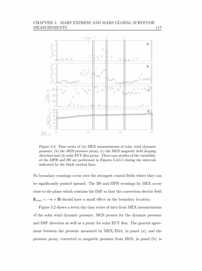
CHAPTER 5. MARS EXPRESS AND MARS GLOBAL SURVEYORMEASUREMENTS 117
a
c
b
d
Figure 5.2: Time series of (a) MEX measurements of solar wind dynamicpressure, (b) the MGS pressure proxy, (c) the MGS magnetic field drapingdirection and (d) solar EUV flux proxy. Three case studies of the variabilityof the MPB and BS are performed in Figures 5.3-5.5 during the intervalsindicated by the black vertical lines.
No boundary crossings occur over the strongest crustal fields where they can
be significantly pushed upward. The BS and MPB crossings by MEX occur
close to the plane which contains the IMF so that the convection electric field
Econv = −v ×B should have a small effect on the boundary location.
Figure 5.2 shows a seven day time series of data from MEX measurements
of the solar wind dynamic pressure, MGS proxies for the dynamic pressure
and IMF direction as well as a proxy for solar EUV flux. The general agree-
ment between the pressure measured by MEX/IMA, in panel (a), and the
pressure proxy, converted to magnetic pressure from MGS, in panel (b), is
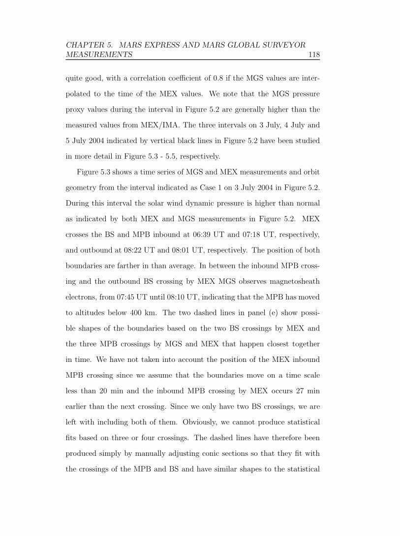
CHAPTER 5. MARS EXPRESS AND MARS GLOBAL SURVEYORMEASUREMENTS 118
quite good, with a correlation coefficient of 0.8 if the MGS values are inter-
polated to the time of the MEX values. We note that the MGS pressure
proxy values during the interval in Figure 5.2 are generally higher than the
measured values from MEX/IMA. The three intervals on 3 July, 4 July and
5 July 2004 indicated by vertical black lines in Figure 5.2 have been studied
in more detail in Figure 5.3 - 5.5, respectively.
Figure 5.3 shows a time series of MGS and MEX measurements and orbit
geometry from the interval indicated as Case 1 on 3 July 2004 in Figure 5.2.
During this interval the solar wind dynamic pressure is higher than normal
as indicated by both MEX and MGS measurements in Figure 5.2. MEX
crosses the BS and MPB inbound at 06:39 UT and 07:18 UT, respectively,
and outbound at 08:22 UT and 08:01 UT, respectively. The position of both
boundaries are farther in than average. In between the inbound MPB cross-
ing and the outbound BS crossing by MEX MGS observes magnetosheath
electrons, from 07:45 UT until 08:10 UT, indicating that the MPB has moved
to altitudes below 400 km. The two dashed lines in panel (e) show possi-
ble shapes of the boundaries based on the two BS crossings by MEX and
the three MPB crossings by MGS and MEX that happen closest together
in time. We have not taken into account the position of the MEX inbound
MPB crossing since we assume that the boundaries move on a time scale
less than 20 min and the inbound MPB crossing by MEX occurs 27 min
earlier than the next crossing. Since we only have two BS crossings, we are
left with including both of them. Obviously, we cannot produce statistical
fits based on three or four crossings. The dashed lines have therefore been
produced simply by manually adjusting conic sections so that they fit with
the crossings of the MPB and BS and have similar shapes to the statistical
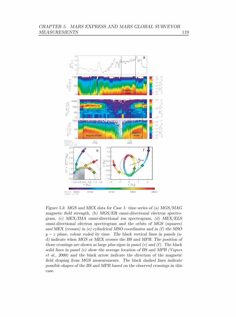
CHAPTER 5. MARS EXPRESS AND MARS GLOBAL SURVEYORMEASUREMENTS 119
a
fe
d
c
b
Magneto- sheath
MagnetosheathMagneto- sheath
BDrape
Figure 5.3: MGS and MEX data for Case 1: time series of (a) MGS/MAGmagnetic field strength, (b) MGS/ER omni-directional electron spectro-gram, (c) MEX/IMA omni-directional ion spectrogram, (d) MEX/ELSomni-directional electron spectrogram and the orbits of MGS (squares)and MEX (crosses) in (e) cylindrical MSO coordinates and in (f) the MSOy − z plane, colour coded by time. The black vertical lines in panels (a-d) indicate when MGS or MEX crosses the BS and MPB. The position ofthose crossings are shown as large plus signs in panel (e) and (f). The blacksolid lines in panel (e) show the average location of BS and MPB (Vigneset al., 2000) and the black arrow indicate the direction of the magneticfield draping from MGS measurements. The black dashed lines indicatepossible shapes of the BS and MPB based on the observed crossings in thiscase.
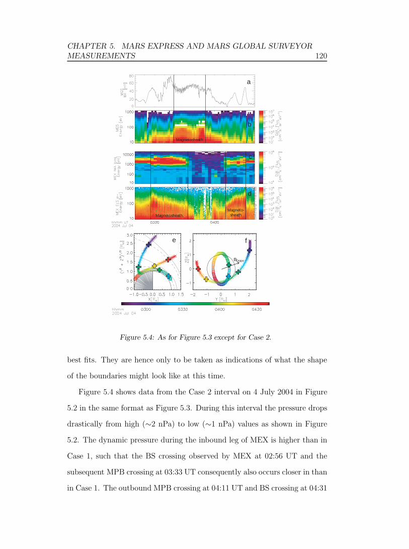
CHAPTER 5. MARS EXPRESS AND MARS GLOBAL SURVEYORMEASUREMENTS 120
Magnetosheath
MagnetosheathMagneto- sheath
a
fe
d
c
b
BDrape
Figure 5.4: As for Figure 5.3 except for Case 2.
best fits. They are hence only to be taken as indications of what the shape
of the boundaries might look like at this time.
Figure 5.4 shows data from the Case 2 interval on 4 July 2004 in Figure
5.2 in the same format as Figure 5.3. During this interval the pressure drops
drastically from high (∼2 nPa) to low (∼1 nPa) values as shown in Figure
5.2. The dynamic pressure during the inbound leg of MEX is higher than in
Case 1, such that the BS crossing observed by MEX at 02:56 UT and the
subsequent MPB crossing at 03:33 UT consequently also occurs closer in than
in Case 1. The outbound MPB crossing at 04:11 UT and BS crossing at 04:31
CHAPTER 5. MARS EXPRESS AND MARS GLOBAL SURVEYORMEASUREMENTS 121
UT are, however, located only slightly closer in compared to the outbound
crossings in Case 1. The pressure during the outbound leg as observed by
MEX had in fact also dropped to only slightly higher values compared to the
values from the outbound leg in Case 1. MGS also observed magnetosheath
electrons during this interval, starting at 03:19 UT and ending at 03:51 UT.
These magnetosheath observations started at roughly the same position in
the y − z plane as in Case 1 (compare panel (g) in Figures 5.4 and 5.3)
but stops much earlier in this case, at a lower SZA, probably due to the fact
that the upstream pressure decreased and the magnetosheath moves outward
again.
Figure 5.5 shows data from the Case 3 interval on 5 July 2004 in Figure
5.2 in the same format as Figure 5.3 and 5.4. At this time the pressure of
the solar wind had decreased to lower values of ∼0.2 nPa as shown both by
the MGS pressure proxy and the MEX measurements in Figure 5.2. The
inbound BS crossing and MPB crossing observed by MEX at 05:45 UT and
06:15 UT, respectively, are still located farther in than average but have
moved out compared to Case 2. The inbound BS crossing actually still oc-
curs slightly farther in compared to the inbound BS crossings in Case 1, which
indicates that factors other than solar wind dynamic pressure are involved
in determining the position of the boundary such as magnetosheath plasma
pressure, crustal fields (possibly on a more global scale since neither of the
crossings occurs directly over strong crustal fields) or EUV flux. The out-
bound MPB crossing at 07:13 UT and BS crossing at 07:32 UT have moved
outward significantly and are now located at larger radius than their average
positions. The outbound MPB and BS crossings by MEX also occur in the
−Econv-hemisphere and are still farther out than average, indicating that the
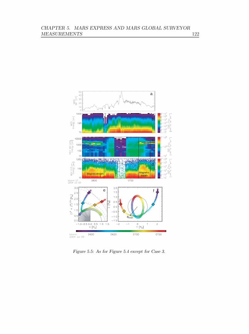
CHAPTER 5. MARS EXPRESS AND MARS GLOBAL SURVEYORMEASUREMENTS 122
Magneto- sheath
Magnetosheath
a
fe
d
c
b
BDrape
Figure 5.5: As for Figure 5.4 except for Case 3.

CHAPTER 5. MARS EXPRESS AND MARS GLOBAL SURVEYORMEASUREMENTS 123
convective electric field has a weak influence on the boundary locations in
this case. MGS observes no magnetosheath plasma at all during this interval.
Evidently, the pressure was simply not high enough to push the MPB and
the magnetosheath down to the altitude of MGS.
To summarize, both the MGS pressure proxy and MEX measurements
indicate that the solar wind undergoes changes in dynamic pressure during
the interval. The boundaries are observed to response in such a way that they
are pushed inward when the dynamic pressure is high, as shown in Figure
5.3. When the dynamic pressure is even higher, as during the inbound part in
Figure 5.4, the boundaries are even farther in. The magnetosheath is in fact
pushed inward to below the 400 km altitude of MGS. But when the pressure
drops, which happens sometimes between 03:51 UT and 04:11 UT in Figure
5.4, the boundaries respond and move outward quickly and we can conclude
that the response time of the plasma environment of Mars to new solar wind
conditions is at least less than 20 min. From Figure 5.5, we conclude that
the boundaries can either take asymmetric forms since the boundaries, during
steady solar wind conditions, are farther out over one hemisphere than the
other, or, that the shape of the boundaries do not follow the average best
fit conic section shape in this case since the inbound and outbound crossings
also occur at different SZAs. The ’asymmetry’ does not seem to depend on
the direction of the convective electric field, which could be a factor which
causes asymmetry. Neither do the boundary crossings take place over strong
crustal fields over which they could be significantly pushed upward. This
leads us to believe that the latter of the two explanations is correct.
CHAPTER 5. MARS EXPRESS AND MARS GLOBAL SURVEYORMEASUREMENTS 124
5.5 Statistical studies with simultaneous mea-
surements
5.5.1 Influence of the solar wind dynamic pressure
In Figure 5.6 we show the result of a statistical study of how the radial
distances of the BS and the MPB vary with solar wind dynamic pressure. We
have used all the crossings observed by MEX during the overlapping mission
time with MGS and extrapolated them to the terminator plane in order
to remove the SZA angle dependence. The boundaries tend to be at higher
altitudes at higher SZAs and in order to compare crossing with each other we
need to remove this dependence and we therefore extrapolate the positions of
all the crossings to the terminator plane. The extrapolation is done using the
same method as described in Vignes et al. (2002) and Crider et al. (2002).
First, the crossings are rotated by 4◦ about the MSO z axis to account for the
perpendicular movement of Mars relative to the solar wind flow direction. A
conic section is then fitted to each crossing of the BS and MPB in the MSO
(x,√
y2 + z2) plane by using the best fit values of the eccentricity ε and X0
from Edberg et al. (2008), varying only the semi-latus rectum L. For each
conic section the terminator distance is then calculated. This method is
not perfect, since the eccentricity of the boundaries can possibly also change
when the governing factors change, but it remains the best we can do for now
in order to remove the SZA dependence. Fitting curves by varying only ε or
only X0 does not give reasonable curves. Crossings that occur either much
closer in than average or far downtail tend to produce fitted curves that pass
through the planet. Varying L and keeping the other parameters fixed gives
more reasonable curves in this sense. We therefore assume ε and X0 to be
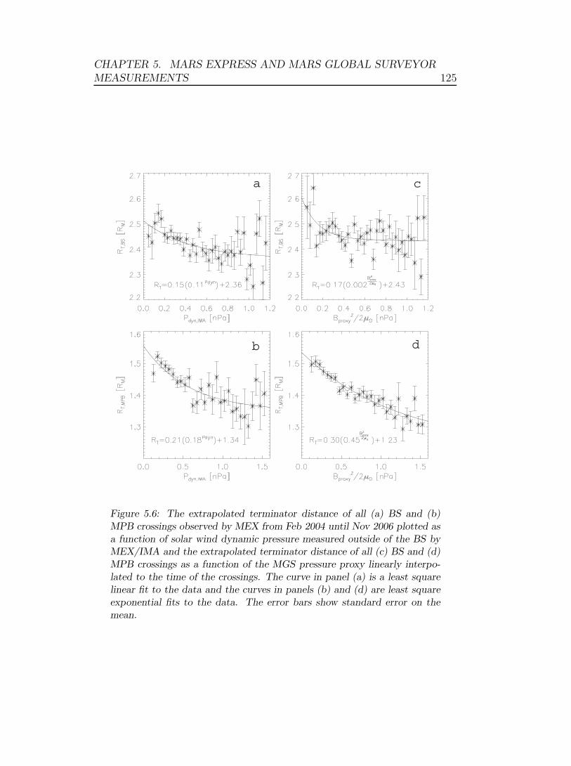
CHAPTER 5. MARS EXPRESS AND MARS GLOBAL SURVEYORMEASUREMENTS 125
a c
b d
Figure 5.6: The extrapolated terminator distance of all (a) BS and (b)MPB crossings observed by MEX from Feb 2004 until Nov 2006 plotted asa function of solar wind dynamic pressure measured outside of the BS byMEX/IMA and the extrapolated terminator distance of all (c) BS and (d)MPB crossings as a function of the MGS pressure proxy linearly interpo-lated to the time of the crossings. The curve in panel (a) is a least squarelinear fit to the data and the curves in panels (b) and (d) are least squareexponential fits to the data. The error bars show standard error on themean.

CHAPTER 5. MARS EXPRESS AND MARS GLOBAL SURVEYORMEASUREMENTS 126
constant.
Figure 5.6, panel (a), shows the extrapolated terminator distances RT
of the BS crossings as a function of upstream solar wind dynamic pressure
Pdyn,IMA as measured by MEX/IMA. The crossings are binned into 0.05 RM
bins and the mean values of the dynamic pressure upstream of all crossings
in each bin is calculated. The error bars show standard error on the mean
(standard deviation divided by number of samples in each bin). There is a
trend to smaller radial distance for higher dynamic pressure, with a corre-
lation coefficient of -0.51, and we fit an exponential curve (solid line) of the
form RT = abPdyn + c, where a, b and c are free parameters, to the data
points. In panel (b) we show the terminator radius of the MPB as a func-
tion of Pdyn,IMA. Again, there is a clear trend to smaller radial distances
for higher Pdyn,IMA, with a correlation coefficient of -0.74, and we fit the
same type of exponential curve to the data points. The error bars at low
radial distance increase which could be an effect of the stronger influence of
the crustal fields at lower altitudes. However, it could also be an effect of
fewer data points in these bins. These two results clearly show that the solar
wind dynamic pressure has an influence on the location of the boundaries,
as would be expected.
We also compare these results to those obtained when we use the MGS
pressure proxy rather than Pdyn,IMA. Panel (c) and (d) show the terminator
radius of the BS and MPB, respectively, as a function of the MGS pressure
proxyB2
proxy
2μ0. The pressure proxy values are linearly interpolated to the time
of the boundary crossings. Surprisingly, there is no obvious trend for the
variation of the BS radius (correlation coefficient of -0.41) whereas the trend
for the MPB is very similar to that in panel (b) (correlation coefficient of

CHAPTER 5. MARS EXPRESS AND MARS GLOBAL SURVEYORMEASUREMENTS 127
-0.93). The lack of a trend for the BS crossings could be explained by the
time difference between the time of the pressure proxy measurement and the
BS crossings, which can be as long as 1 hour. The BS is expected to move on
time scales much shorter than that. The error bars are quite large, however,
and including them, then the results are not so discrepant. For the MPB we
should have the same problem with the time difference but the results in panel
(b) and (d) are still very similar, which rather disproves the argument above,
if we assume that the BS and MPB move on the same timescales. It is also
likely that the MPB and the BS can simply respond differently to changes
in the solar wind dynamic pressure. The pressure proxy and the measured
pressure values do not match up perfectly and this could be an indication
of an unknown compression factor between the solar wind dynamic pressure
outside the BS/MPB and the magnetic pressure inside the MPB.
It is also possible that when the BS is at very low radial distances the
crustal magnetic fields become more important while at the same time the
dynamic pressure becomes less important. The dynamic pressure can only
push the boundary down to a certain altitude before the magnetic pressure
from the crustal fields together with the plasma pressure inside of the BS be-
come too high and the trend of a lower radial distance for a higher dynamic
pressure vanishes. Similarly, when the BS is at very high radial distances
the IMF direction could become more important while at the same time
the dynamic pressure becomes less important. Inclusion of crossings that
occur when other parameters, such as IMF direction, solar EUV flux and
crustal magnetic fields, are kept approximately constant would be a way to
decrease the error bars and get clearer trends. Unfortunately, the number
of data points in each bin drops drastically by doing those selections. How-
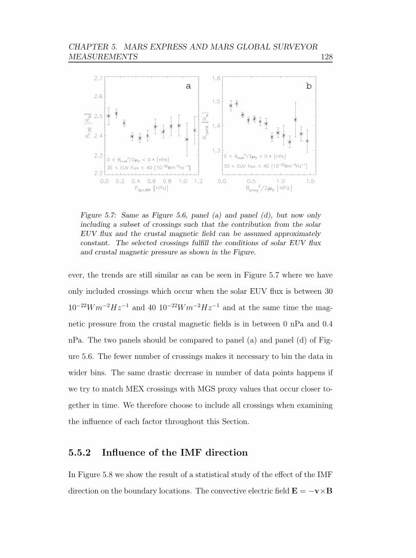
CHAPTER 5. MARS EXPRESS AND MARS GLOBAL SURVEYORMEASUREMENTS 128
a b
Figure 5.7: Same as Figure 5.6, panel (a) and panel (d), but now onlyincluding a subset of crossings such that the contribution from the solarEUV flux and the crustal magnetic field can be assumed approximatelyconstant. The selected crossings fulfill the conditions of solar EUV fluxand crustal magnetic pressure as shown in the Figure.
ever, the trends are still similar as can be seen in Figure 5.7 where we have
only included crossings which occur when the solar EUV flux is between 30
10−22Wm−2Hz−1 and 40 10−22Wm−2Hz−1 and at the same time the mag-
netic pressure from the crustal magnetic fields is in between 0 nPa and 0.4
nPa. The two panels should be compared to panel (a) and panel (d) of Fig-
ure 5.6. The fewer number of crossings makes it necessary to bin the data in
wider bins. The same drastic decrease in number of data points happens if
we try to match MEX crossings with MGS proxy values that occur closer to-
gether in time. We therefore choose to include all crossings when examining
the influence of each factor throughout this Section.
5.5.2 Influence of the IMF direction
In Figure 5.8 we show the result of a statistical study of the effect of the IMF
direction on the boundary locations. The convective electric field E = −v×B

CHAPTER 5. MARS EXPRESS AND MARS GLOBAL SURVEYORMEASUREMENTS 129
should cause the ions to go out into the solar wind and cause massloading of
solar wind on one side of the planet thereby lifting the boundaries upward,
whereas the ions on the other side go back into the planet. In panels (a) and
(b) the distribution of the radial distances of BS crossings at northern and
southern latitudes of Mars, respectively, are shown, divided into whether
the crossing occur during locally upward (+E) or locally downward (−E)
convective electric field. The direction of the magnetic field is obtained from
the MGS draping proxy. In panel (c) and (d) the distribution is shown
for the MPB. The radial distances of the crossings are extrapolated to the
terminator plane. In panel (a), the mean value of RT for the BS crossings
that occur in the +E-hemisphere and at northern latitudes is 2.48±0.01 RM
(plus or minus standard error of the mean) and is ∼135 km higher compared
to that in the −E-hemisphere at northern latitudes, 2.44 ± 0.01 RM . The
mean values are significantly different according to a Student’s t-test at a
95% confidence level. This difference is also observed for the crossings that
occur at southern latitudes, in panel (b), and the difference is also significant
according to a Student’s t-test at a 95% confidence level. The southern
latitude mean distances are 2.45±0.01 RM in the +E-hemisphere compared
to 2.41 ± 0.01 RM in the −E-hemisphere, a difference of ∼135 km.
For the MPB, Figure 5.8, panel (c), there is also a significant (according
to a Student’s t-test at a 95% confidence level) difference of ∼135 km be-
tween the mean values of the +E and −E hemisphere crossings at northern
latitudes, 1.41± 0.01 RM compared to 1.37± 0.01 RM . But for the crossings
that occur at southern latitudes, in panel (d), the situation is reversed. The
+E hemisphere crossings have a ∼200 km lower mean value than the −E
hemisphere crossings, 1.40±0.01 RM compared to 1.46±0.01 RM . The south-
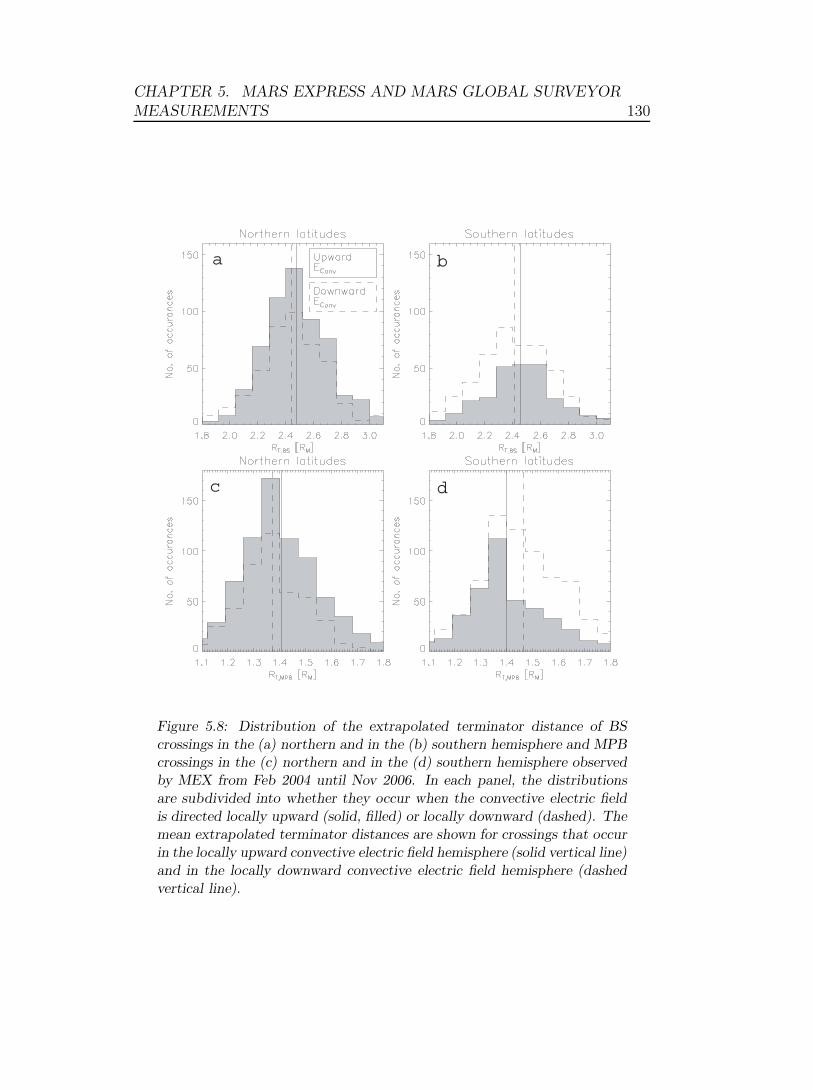
CHAPTER 5. MARS EXPRESS AND MARS GLOBAL SURVEYORMEASUREMENTS 130
a b
dc
Figure 5.8: Distribution of the extrapolated terminator distance of BScrossings in the (a) northern and in the (b) southern hemisphere and MPBcrossings in the (c) northern and in the (d) southern hemisphere observedby MEX from Feb 2004 until Nov 2006. In each panel, the distributionsare subdivided into whether they occur when the convective electric fieldis directed locally upward (solid, filled) or locally downward (dashed). Themean extrapolated terminator distances are shown for crossings that occurin the locally upward convective electric field hemisphere (solid vertical line)and in the locally downward convective electric field hemisphere (dashedvertical line).
CHAPTER 5. MARS EXPRESS AND MARS GLOBAL SURVEYORMEASUREMENTS 131
ern hemisphere MPB apparently reacts differently to an upward/downward
convective electric field compared to the northern hemisphere, on average.
It should be noted that the scatter in the extrapolated terminator distances
is large and there are uncertainties involved in this study, e.g. the IMF di-
rection is not determined perfectly, but only through a proxy and the time
difference between the proxy value and the crossing has not been taken into
account.
5.6 Influence of the crustal magnetic fields
In order to investigate the influence of the crustal magnetic fields we only
use MEX measurements. The crustal fields have previously been shown to
influence the boundaries by using MGS measurements and also MEX mea-
surements on their own (Crider et al., 2002; Brain et al., 2005; Franz et al.,
2006b; Edberg et al., 2008). However, no previous study has used such a large
data set of crossings as we have in this study and we can now for the first
time produce global maps of the radial distances of the boundaries. Panel
(a) and (b) in Figure 5.9 show two global 10◦ × 10◦ longitude-latitude maps
colour coded by the radial distances of the BS and MPB, respectively. All
crossings from Feb 2004 until Jan 2009 from the dayside of Mars are used and
the mean of the radial distances of all crossings within each bin are shown.
Bins with less than two crossings are coloured black. Note that the strongest
crustal fields are located in the southern hemisphere at longitudes between
90◦ and 270◦ (Connerney et al., 2005). The map of the BS crossings, panel
(a), shows no distinct influence of the crustal magnetic fields on the altitude
of the boundary, i.e. there is no specific region where the boundary is at

CHAPTER 5. MARS EXPRESS AND MARS GLOBAL SURVEYORMEASUREMENTS 132
a
b
Figure 5.9: Longitude-latitude maps colour coded by the extrapolated ter-minator distance RT of the (a) BS and (b) MPB. Only dayside crossingswere used. Black bins means that there were less than two crossings inthat region.

CHAPTER 5. MARS EXPRESS AND MARS GLOBAL SURVEYORMEASUREMENTS 133
larger radial distance than elsewhere and which also corresponds to a region
of strong crustal fields. There are, unfortunately, many empty bins at south-
ern latitudes where the crustal fields are strongest. However, the mean value
of RT of all the dayside BS crossings in the northern hemisphere is 2.45 RM
compared to 2.49 RM in the southern hemisphere and in the bottom rows of
panel (a), at southern latitudes, there is a weak tendency that the crossings
are at higher distances. The difference is statistically significant according
to a Student’s t-test at 95% confidence level. This difference is smaller than
the difference presented in Edberg et al. (2008) where MGS crossings where
used. The accuracy in this study should, however, be better due to the much
larger data set.
The influence of the crustal magnetic fields on the MPB is much clearer.
In panel (b) of Figure 5.9 there is a large area at southern latitudes between
longitudes from ∼90◦ to ∼270◦, where the MPB at occurs larger radial dis-
tances than elsewhere. This region corresponds very closely to the region
where the strongest crustal fields are located. Also, at latitudes above −30◦
and at longitudes between 0◦ and 90◦ there is a less prominent but still visible
area of higher MPB which corresponds to a region of intermediately strong
crustal fields.
In Figure 5.10 we show the extrapolated terminator distances of all the
dayside crossings of the BS and MPB plotted as functions of magnetic pres-
sure contributed from the crustal anomalies. The magnetic field strength is
estimated by using the model from Cain et al. (2003) and calculate the field
strength at 100 positions evenly spaced on a 10◦×10◦ longitude-latitude grid
centered radially below each crossings at 400 km. The mean over these 100
values are then taken as the field strength for each individual crossing. We
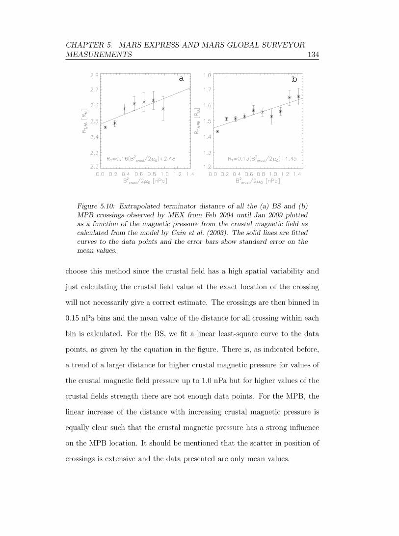
CHAPTER 5. MARS EXPRESS AND MARS GLOBAL SURVEYORMEASUREMENTS 134
a b
Figure 5.10: Extrapolated terminator distance of all the (a) BS and (b)MPB crossings observed by MEX from Feb 2004 until Jan 2009 plottedas a function of the magnetic pressure from the crustal magnetic field ascalculated from the model by Cain et al. (2003). The solid lines are fittedcurves to the data points and the error bars show standard error on themean values.
choose this method since the crustal field has a high spatial variability and
just calculating the crustal field value at the exact location of the crossing
will not necessarily give a correct estimate. The crossings are then binned in
0.15 nPa bins and the mean value of the distance for all crossing within each
bin is calculated. For the BS, we fit a linear least-square curve to the data
points, as given by the equation in the figure. There is, as indicated before,
a trend of a larger distance for higher crustal magnetic pressure for values of
the crustal magnetic field pressure up to 1.0 nPa but for higher values of the
crustal fields strength there are not enough data points. For the MPB, the
linear increase of the distance with increasing crustal magnetic pressure is
equally clear such that the crustal magnetic pressure has a strong influence
on the MPB location. It should be mentioned that the scatter in position of
crossings is extensive and the data presented are only mean values.
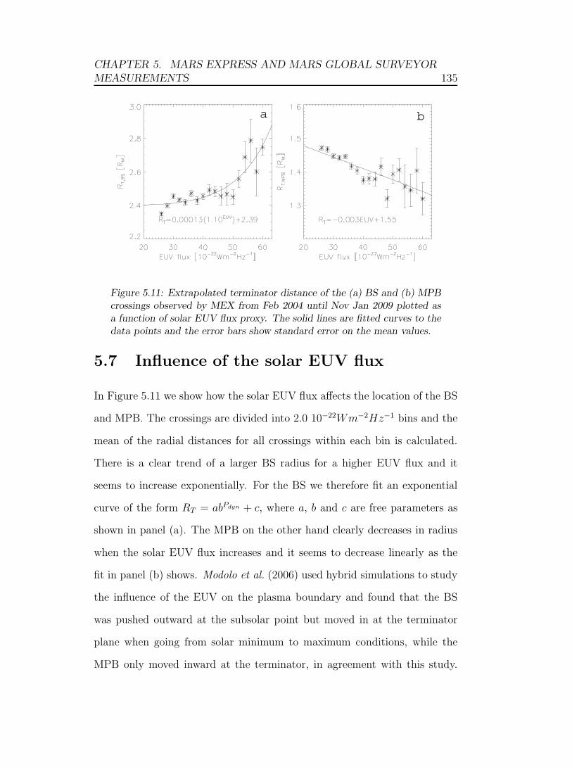
CHAPTER 5. MARS EXPRESS AND MARS GLOBAL SURVEYORMEASUREMENTS 135
a b
Figure 5.11: Extrapolated terminator distance of the (a) BS and (b) MPBcrossings observed by MEX from Feb 2004 until Nov Jan 2009 plotted asa function of solar EUV flux proxy. The solid lines are fitted curves to thedata points and the error bars show standard error on the mean values.
5.7 Influence of the solar EUV flux
In Figure 5.11 we show how the solar EUV flux affects the location of the BS
and MPB. The crossings are divided into 2.0 10−22Wm−2Hz−1 bins and the
mean of the radial distances for all crossings within each bin is calculated.
There is a clear trend of a larger BS radius for a higher EUV flux and it
seems to increase exponentially. For the BS we therefore fit an exponential
curve of the form RT = abPdyn + c, where a, b and c are free parameters as
shown in panel (a). The MPB on the other hand clearly decreases in radius
when the solar EUV flux increases and it seems to decrease linearly as the
fit in panel (b) shows. Modolo et al. (2006) used hybrid simulations to study
the influence of the EUV on the plasma boundary and found that the BS
was pushed outward at the subsolar point but moved in at the terminator
plane when going from solar minimum to maximum conditions, while the
MPB only moved inward at the terminator, in agreement with this study.
CHAPTER 5. MARS EXPRESS AND MARS GLOBAL SURVEYORMEASUREMENTS 136
The data used in this study are all taken during the declining phase of the
solar cycle and during solar minimum (years 2004 - 2009) and we cannot yet
determine how the EUV flux at solar maximum will affect the boundaries.
5.8 Summary and conclusions
We have shown case studies and statistical studies using single as well as two-
spacecraft simultaneous and non-simultaneous measurements of how the solar
wind dynamic pressure, the IMF direction, the crustal magnetic fields and
the solar EUV flux affects the BS and MPB. We have produced expressions
for how these factors influence the boundaries which enables us to determine
their relative importance. We have not been able to study the influence of
the solar wind magnetosonic Mach number since we do not have upstream
magnetic field measurements. At Venus for instance, the magnetosonic Mach
number has been shown to be of importance in determining the position of
the BS (Russell et al., 1988) and it is reasonable to assume that it should
play a role at Mars too.
The case studies (Figures 5.3 - 5.5) employ simultaneous MEX and MGS
measurements during an interval when the solar wind dynamic pressure
changes from high to low and the dynamic pressure is assumed to have the
main influence on the boundary locations. The effect of the high pressure
solar wind on the boundaries is indeed observed to be an inward movement
of both boundaries. The MPB is in fact pushed closer to the planet than
the altitude of MGS (∼400 km). Both BS and the MPB remains compressed
until the solar wind dynamic pressure has decreased back to lower values. We
can provide an upper limit of ∼20 min for how long it takes for the Martian
CHAPTER 5. MARS EXPRESS AND MARS GLOBAL SURVEYORMEASUREMENTS 137
plasma environment to adapt to new upstream solar wind conditions (Figure
5.4). The shapes of the boundaries seem to alter during this time as well
as indicated by near-simultaneous measurements of the MPB by MEX and
MGS (Figure 5.4, panel (f)). The BS, which is only observed by MEX and
separated in time from the inbound to the outbound by ∼1.5 hours, making
it far from simultaneous, might also change its shape (Figure 5.3 and Figure
5.6, panel (f)). However, the BS is expected to move on time scales much
shorter than this and this shape estimate is therefore very uncertain.
A statistical study of how the position of all MEX boundary crossings
during the time of the mission overlap with MGS (Feb 2004 - Nov 2006)
varies with solar wind dynamic pressure has also been performed (Figure
5.6). The boundaries are, on average, found to decrease exponentially in
altitude with increasing pressure. Very similar results are produced when
using the solar wind dynamic pressure as determined from a proxy from
MGS data and by direct measurements from MEX. The statistical studies
in Figure 5.6 also provide confidence in the accuracy of the MGS and MEX
measurement, which independently give very similar result. However, for the
BS the method of using the MEX measurements give a seemingly clearer
result to how the radial distance decrease with increasing dynamic pressure.
If the MGS pressure is used, the trend is less clear but still visible. The
BS could possibly move on shorter time scales than the MPB and the MGS
pressure proxy has a too poor time resolution which would mean that the
MGS proxy is not suitable for studying the variation of MEX BS crossings
with dynamic pressure. Also, the trend for the MPB appears clearer if the
MGS pressure proxy is used rather than if the MEX/IMA measurements are
used. These results indicate that the BS and MPB do not respond in exactly
CHAPTER 5. MARS EXPRESS AND MARS GLOBAL SURVEYORMEASUREMENTS 138
the same way when facing changes in the upstream solar wind conditions.
A statistical study of how the boundaries react to different directions of
convective electric field has also been performed (Figure 5.8) by using two-
spacecraft measurements. We show that the BS has a 135 km larger average
radial distance in the hemisphere of locally upward convective electric field
compared to that in the hemisphere of locally downward convective electric
field. The same difference is valid for the MPB but only in the northern
hemisphere where the boundary during locally upward convective electric
field has a 135 km larger average radial distance compared to when locally
downward. In the southern latitudes, the situation seems to be reversed and
the MPB is closer to the planet in the hemisphere of locally upward electric
field, by 200 km on average. The difference is possibly due to the influence of
the crustal magnetic fields, which are strongest in the southern hemisphere
and disturb the (weak) effect of asymmetric massloading. Overall, the IMF
direction has a weak influence on the boundaries if compared to other factors.
We also confirm observations, by using MEX measurements only, that
the crustal fields affect both the MPB and the BS strongly by providing
additional magnetic pressure. The radial distances of the BS and the MPB
increase linearly with the crustal magnetic pressure.
The EUV flux, which ionises neutrals in the extended exosphere of Mars
and increases the plasma pressure, is also shown to have a strong influence
on both boundaries. The BS radius increases exponentially with increasing
EUV flux while the MPB radius is observed to decrease linearly with increas-
ing EUV flux. An explanation for this could be that the plasma pressure in
the magnetosheath, in between the BS and the MPB, could be significantly
increased with increasing EUV flux which could cause the BS to move out-

CHAPTER 5. MARS EXPRESS AND MARS GLOBAL SURVEYORMEASUREMENTS 139
ward and the MPB to move inward. We have not found a correlation between
solar EUV flux and high dynamic pressure which could have explained the
result for the MPB.
There are several sources of error involved in this study, which causes
scatter in the location of the boundaries. These errors include the time delay
between MGS proxy values/upstream MEX measurements and the boundary
crossings, the unknown x-component of the magnetic field and the unknown
upstream magnetosonic Mach number. A sheared solar wind flow would also
distort the results. The solar EUV proxy could also introduce an error since it
is extrapolated from Earth and so can also the extrapolation of the boundary
distances to the terminator plane do.
We can compare our observations of which factors control the location the
plasma boundaries to models. The IMF direction is generally shown to be of
importance in hybrid models which take kinetic effects in to account (Boßwet-
ter et al., 2004; Modolo et al., 2006), but is not really important in this study.
Other factors seem to be more important. However, the IMF direction is, as
stated before, not directly measured but rather determined through a proxy,
which introduces errors. The dynamic pressure dependence is in reasonable
agreement with models, both hybrid and MHD models (Boßwetter et al.,
2004; Modolo et al., 2006). The crustal fields have not been studied exten-
sively in models but will most likely become included in most future studies.
Harnett and Winglee (2003) have performed such a study and showed that
the MPB is affected to a large extent, which is in agreement with the results
presented here, while the BS was not affected, which is in disagreement. The
solar EUV flux dependence has been studied by Modolo et al. (2006) who
found a weak dependence, in contrast to the results here. It should be noted
CHAPTER 5. MARS EXPRESS AND MARS GLOBAL SURVEYORMEASUREMENTS 140
that almost all models obtain very different results in terms of plasma escape
rates as well as boundary locations, when the same input conditions are used
(Brain et al., 2009).
In summary, quantitative expressions for the main factors the affect that
BS and the MPB have been produced. The factors that mainly affect the
MPB include the solar wind dynamic pressure, crustal magnetic fields and
solar EUV flux while the IMF direction has a weaker influence. For the BS,
the crustal magnetic fields, the solar wind dynamic pressure and the solar
EUV are again the main controlling factors while the IMF direction plays a
minor role.
Chapter 6Conclusions & future work
6.1 Conclusions
This Thesis has focused on the solar wind interaction with Mars and the
boundaries and regions that form as a result of that interaction. We have
studied the location, shape and dynamics of the MPB and BS and also which
parameters that influence the properties of the boundaries. Throughout these
studies we have used single spacecraft measurements as well as simultaneous
and non-simultaneous two-spacecraft measurements.
In Chapter 3 we have used MGS data to produce best-fit statistical models
of the average shape of both the MPB and BS. We have also studied the
influence of the crustal magnetic fields on the two boundaries and found that
the MPB is pushed upward over specific regions where the crustal magnetic
field of Mars is particularly strong. Where the crustal magnetic fields are even
stronger, the MPB is pushed to even higher altitudes. The BS was found to
be at higher altitudes over the entire southern hemisphere, where the crustal
magnetic fields are mainly located, but there was no observable difference
between strong or intermediately strong crustal magnetic field regions.
141
CHAPTER 6. CONCLUSIONS & FUTURE WORK 142
The average shapes of both boundaries take the form of conic sections
which has previously been determined. We have, however, extended the
previous studies by including more data points which has increased the sta-
tistical accuracy as well as constrained the shape of the MPB by introducing
a new method for performing the fitting. The new method takes into account
the fact that there are no MPB crossings at low SZAs which otherwise intro-
duces an error in the fitting technique. The previous models have had their
lowest altitudes at a SZA of ∼45◦ rather than at 0◦ which would have been
expected. We therefore perform a fitting where we fix the subsolar altitude
to a value based on the lowest altitude of the previous fits. The result is a
more realistic model of the MPB. We have also studied the magnetic field
strength inside the MPB and found that it increases toward the dayside as
well as when the MPB is pushed closer to the planet.
In Chapter 4 we have used simultaneous measurement from Rosetta and
MEX to study the behavior of the MPB and BS during low and high solar
wind pressure. The Rosetta swingby of Mars, which took place in Febru-
ary 2007, enabled the first near-simultaneous two-spacecraft study of plasma
boundaries at Mars as well as an opportunity for using Rosetta as a solar
wind monitor while MEX sampled the MPB and BS. The near-simultaneous
BS and MPB measurements took place within an interval of ∼3 hours, dur-
ing which the solar wind was quiet and slow with a normal density. We use
the near-simultaneous boundary crossings to confirm the previously mod-
elled shapes and find that both the MPB and the BS shape are in reasonable
agreement with the models. The MPB is found at its average location as
would be expected during quiet solar wind conditions. The BS is, however,
significantly compressed during this interval, but still with a conic section
CHAPTER 6. CONCLUSIONS & FUTURE WORK 143
shape.
A day after the CA of Rosetta a high pressure solar wind region is observed
to pass by Mars during a ∼24 hour interval. As Rosetta monitors the solar
wind and the IMF downstream of Mars, MEX observes how the MPB and BS
become asymmetric in shape. The observed boundary in the northern/dawn
hemisphere is closer in than the observed boundary in the southern/dusk
hemisphere. We test various factors which could cause the asymmetry, such
as the IMF direction and crustal magnetic fields, without finding a good
explanation. The BS altitude clearly increases on one side of the planet even
though the solar wind pressure increases which is rather unexpected. At the
same time, a significant fraction of ionospheric ions are observed to accelerate
away from the planet in the hemisphere where the boundaries are at lower
altitudes. We therefore suggest that the observed boundary asymmetry is
related to the ionospheric outflow as the thermal plasma pressure decreases
when plasma is swept away.
In Chapter 5 we use both simultaneous and non-simultaneous two-spacecraft
measurements from MEX and MGS to study some factors which have been
suggested to control the altitude of the MPB and BS. First, we introduce
previously produced proxies of the solar wind dynamic pressure and IMF
direction based on MGS measurements as well as a proxy of the EUV flux
based on F10.7 measurements at Earth. We compare the solar wind dynamic
pressure proxy with the measured solar wind dynamic pressure from the IMA
instrument onboard MEX and find that they are in reasonable agreement.
We use the proxies to present a case study during an interval when the solar
wind dynamic pressure is observed to be the governing factor of the move-
ment of the MPB and BS. The boundaries move to lower altitudes as the

CHAPTER 6. CONCLUSIONS & FUTURE WORK 144
solar wind dynamic pressure increases and subsequently to higher altitudes
when the pressure decreases. This case study also gives an indication of the
time scale of which the plasma boundaries move when the dynamic pressure
changes, which is found to be less than 20 min.
Furthermore, by using the three proxies and the measured upstream dy-
namic pressure, we produce analytical expressions of the altitude of the
boundaries, in terms of terminator distance, as functions of solar wind dy-
namic pressure, solar EUV flux and crustal magnetic fields. We also study
the influence of the IMF direction. The result shows that both the MPB and
the BS are mainly controlled by the solar wind dynamic pressure, crustal
magnetic fields and solar EUV flux while the IMF direction plays a minor
role.
6.2 Future work
What is left for the future in terms of studies of plasma boundaries at Mars
include determining in more detail the pressure balance between the MPB
and the underlying MPR and how that effects the BS location. Also, the
boundaries have not yet been studied during solar maximum and their be-
havior during very high solar EUV flux is unknown. Related to this is the
time scale on which these boundaries, and regions, adapt to changing solar
wind conditions. This time scale is expected to be on the order of minutes,
or even seconds, and has not been properly explored. We do touch upon
the subject in Chapter 4 and 5 but not in any great detail. Seasonal effects
have not been studied in any detail in this Thesis and have been left for the
future. Since the Mars rotation axis is tilted, the boundaries could possibly

CHAPTER 6. CONCLUSIONS & FUTURE WORK 145
be located farther in over the summer hemisphere compared to the winter
hemisphere.To produce a functional fit of the boundaries is also desired. The
published models of the boundaries have so far only involved producing best-
fit statistical shapes but to have a model as a function of solar wind pressure,
crustal magnetic field strength and solar EUV flux, for instance, would be
even better. This is something that could be extracted from the quantitative
expressions presented in Chapter 5 in a future study.
While the location and shape of the Martian plasma boundaries have been
extensively explored by several single spacecraft missions in the past, there
has not been any dedicated multi-spacecraft mission for studies of the plasma
boundaries. For the future, such missions would be very advantageous in the
study of the solar wind interaction with Mars. At Earth, multi-spacecraft
missions such as Cluster and Themis have been very successful as they can
resolve spatial from temporal variations in the plasma environment. No such
dedicated mission is currently planned for Mars but there might be more
occasions when two or even three individual spacecraft missions are present
at the same time, with plasma instruments onboard. The Maven mission
from NASA is planned to be launched in 2013 and the Russian Phobos-
Grunt mission will be launched at approximately the same time which will
include a Chinese orbiter, Yinghuo-1, as well. If MEX is still alive at Mars
when these three spacecraft arrive there will be an unprecedented coverage
of plasma measurements around Mars.
To have a long-term upstream solar wind monitor at Mars would make
it possible to study the influence of different solar wind conditions on the
Martian plasma environment in more detail. At present, upstream solar
wind monitoring spacecraft at the Earth can be used, to some extent, even for
CHAPTER 6. CONCLUSIONS & FUTURE WORK 146
Mars. Especially when Mars and Earth are aligned on a straight Mars-Earth-
Sun line, larger solar events such as coronal mass ejections can be tracked
from the Earth to Mars. Also, during solar minimum conditions when the
Sun is relatively quiet, most corotating interaction regions (CIRs) seen at
Earth can easily be traced to Mars, even when the two planets are separated
by as much as ∼120◦ in longitude from each other. This is something which
is presently being explored in a current study where we use Stereo and ACE
data to trace CIRs to Mars. The aim is to determine what the effects these
high pressure solar wind regions have on the plasma environment at Mars.
Other interesting scientific questions which still need to be addressed in
the future includes the physics of the plasma environment close to the crustal
magnetic fields. With both magnetic field and electric field instruments as
well as ion and electron sensors several physical mechanisms such as recon-
nection and auroral emissions could be studied in more detail above regions
of strong crustal magnetic fields. The evolution of the atmosphere of Mars
is also one of the main scientific questions to be addressed. For instance, the
outflow of the cold ion population has not been studied yet which is impor-
tant for determining how the atmosphere has evolved in the past. All this
could possibly be explored with the multi-instrument missions of Maven and
Phobos-Grunt/Yinghuo-1 during the next decade.
Bibliography
Acuna, M. H., J. E. P. Connerney, P. Wasilewski, R. P. Lin, K. A. Ander-son, C. W. Carlson, J. McFadden, D. W. Curtis, D. Mitchell, H. Reme,C. Mazelle, J. A. Sauvaud, C. D’Uston, A. Cros, J. L. Medale, S. J. Bauer,P. Cloutier, M. Mayhew, D. Winterhalter, and N. F. Ness (1998), Magneticfield and plasma observations at Mars: Initial results of the Mars GlobalSurveyor mission, Science, 279, 1676–1680.
Acuna, M. H., J. E. P. Connerney, N. F. Ness, R. P. Lin, D. Mitchell, C. W.Carlson, J. McFadden, K. A. Anderson, H. Reme, C. Mazelle, D. Vignes,P. Wasilewski, and P. Cloutier (1999), Global distribution of crustal mag-netization discovered by the Mars Global Surveyor MAG/ER experiment,Science, 284, 790–793.
Arkani-Hamed, J. (2004), A coherent model of the crustal magnetic field ofMars, J. Geophys. Res., 109, E09,005, doi:10.1029/2004JE002265.
Auster, H. U., I. Apathy, G. Berghofer, A. Remizov, R. Roll, K.-H. For-nacon, K.-H. Glassmeier, G. Haerendel, I. Hejja, E. Kuhrt, W. Magnes,D. Moehlmann, U. Motschmann, I. Richter, H. Rosenbauer, C. T. Russell,J. Rustenbach, K. Sauer, K. Schwingenschuh, I. Szemerey, and R. Waesch(2007), ROMAP: Rosetta Magnetometer and Plasma Monitor, Space Sci.Rev., 128, 221–240, doi:10.1007/s11214-006-9033-x.
Barabash, S., R. Lundin, H. Andersson, K. Brinkfeldt, A. Grigoriev,H. Gunell, M. Holmstrom, M. Yamauchi, K. Asamura, P. Bochsler,P. Wurz, R. Cerulli-Irelli, A. Mura, A. Milillo, M. Maggi, S. Orsini, A. J.Coates, D. R. Linder, D. O. Kataria, C. C. Curtis, K. C. Hsieh, B. R.Sandel, R. A. Frahm, J. R. Sharber, J. D. Winningham, M. Grande,E. Kallio, H. Koskinen, P. Riihela, W. Schmidt, T. Sales, J. U. Kozyra,N. Krupp, J. Woch, S. Livi, J. G. Luhmann, S. McKenna-Lawlor, E. C.Roelof, D. J. Williams, J.-A. Sauvaud, A. Fedorov, and J.-J. Thocaven(2006), The Analyzer of Space Plasmas and Energetic Atoms (ASPERA-
147
BIBLIOGRAPHY 148
3) for the Mars Express mission, Space Sci. Rev., 126, 113–164, doi:10.1007/s11214-006-9124-8.
Barabash, S., A. Fedorov, R. Lundin, and J.-A. Sauvaud (2007),Martian Atmospheric Erosion Rates, Science, 315, 501–503, doi:10.1126/science.1134358.
Bertucci, C., C. Mazelle, D. H. Crider, D. Vignes, M. H. Acuna, D. L.Mitchell, R. P. Lin, J. E. P. Connerney, H. Reme, P. A. Cloutier, N. F.Ness, and D. Winterhalter (2003), Magnetic field draping enhancement atthe Martian magnetic pileup boundary from Mars global surveyor obser-vations, Geophys. Res. Lett., 30 (2), 1099, doi:10.1029/2002GL015713.
Bertucci, C., C. Mazelle, M. H. Acuna, C. T. Russell, and J. A. Slavin (2005),Structure of the magnetic pileup boundary at Mars and Venus, J. Geophys.Res., 110, A01,209, doi:10.1029/2004JA010592.
Boesswetter, A., U. Auster, I. Richter, M. Franz, B. Langlais, S. McKenna-Lawlor, S. Simon, U. Motschmann, K. H. Glassmeier, N. J. T. Edberg, andR. Lundin (2009), Rosetta swing-by at mars - an analysis of the romapmeasurements in comparison with results of 3-d multi-ion hybrid simula-tions and mex/aspera-3 data, Ann. Geophys., 27 (6), 2383–2398.
Boßwetter, A., T. Bagdonat, U. Motschmann, and K. Sauer (2004), Plasmaboundaries at Mars: a 3-D simulation study, Ann. Geophys., 22, 4363–4379.
Brain, D., S. Barabash, A. Boesswetter, S. Bougher, S. Brecht, G. Chanteur,D. Crider, E. Dubinin, X. Fang, M. Fraenz, J. Halekas, E. Harnett,M. Holmstrom, E. Kallio, H. Lammer, S. Ledvina, M. Liemohn, K. Liu,J. Luhmann, Y. Ma, R. Modolo, A. Nagy, U. Motschmann, H. Nilsson,H. Shinagawa, S. Simon, and N. Terada (2009), A comparison of globalmodels for the solar wind interaction with mars, Icarus, In Press, doi:10.1016/j.icarus.2009.06.030.
Brain, D. A., F. Bagenal, M. H. Acuna, and J. E. P. Connerney (2003),Martian magnetic morphology: Contributions from the solar wind andcrust, J. Geophys. Res., 108 (A12), 1424, doi:10.1029/2002JA009482.
Brain, D. A., J. S. Halekas, R. Lillis, D. L. Mitchell, R. P. Lin, and D. H.Crider (2005), Variability of the altitude of the Martian sheath, Geophys.Res. Lett., 32, L18,203, doi:10.1029/2005GL023126.
Brain, D. A., D. L. Mitchell, and J. S. Halekas (2006), The magnetic fielddraping direction at Mars from April 1999 through August 2004, Icarus,182, 464–473, doi:10.1016/j.icarus.2005.09.023.
BIBLIOGRAPHY 149
Brecht, S. H., and S. A. Ledvina (2006), The Solar Wind Interaction Withthe Martian Ionosphere/Atmosphere, Space Sci. Rev., 126, 15–38, doi:10.1007/s11214-006-9084-z.
Burch, J. L., R. Goldstein, T. E. Cravens, W. C. Gibson, R. N. Lundin, C. J.Pollock, J. D. Winningham, and D. T. Young (2007), RPC-IES: The Ionand Electron Sensor of the Rosetta Plasma Consortium, Space Sci. Rev.,128, 697–712, doi:10.1007/s11214-006-9002-4.
Cain, J. C., B. B. Ferguson, and D. Mozzoni (2003), An n = 90 internalpotential function of the Martian crustal magnetic field, J. Geophys. Res.,108 (E2), 5008, doi:10.1029/2000JE001487.
Carlsson, E., D. Brain, J. Luhmann, S. Barabash, A. Grigoriev, H. Nilsson,and R. Lundin (2008), Influence of IMF draping direction and crustalmagnetic field location on Martian ion beams, Planet. and Space Sci., 56,861–867, doi:10.1016/j.pss.2007.12.016.
Chapman, S. (1931a), The absorption and dissociative or ionizing effect ofmonochromatic radiation in an atmosphere on a rotating earth, Proc. ofthe Phys. Soc., 43, 26–45, doi:10.1088/0959-5309/43/1/305.
Chapman, S. (1931b), The absorption and dissociative or ionizing effect ofmonochromatic radiation in an atmosphere on a rotating earth part II.Grazing incidence, Proc. of the Phys. Soc., 43, 483–501, doi:10.1088/0959-5309/43/5/302.
Connerney, J. E. P., M. H. Acuna, N. F. Ness, G. Kletetschka, , D. L.Mitchell, R. P. Lin, and H. Reme (2005), Tectonic implications of Marscrustal magnetism, Proc. Natl. Acad. Sci., 102 (42), 14,970–14,975, doi:10.1073/pnas.0507469102.
Crider, D., M. Acuna, J. Connerney, D. Mitchell, R. Lin, P. Cloutier,H. Reme, C. Mazelle, D. Brain, N. Ness, and S. Bauer (2001), Magneticfield draping around Mars: Mars Global Surveyor results, Adv. Space Res.,27, 1831–1836.
Crider, D. H., M. H. Acuna, J. E. P. Connerney, D. Vignes, N. F. Ness,A. M. Krymskii, T. K. Breus, H. Reme, C. Mazelle, D. L. Mitchell, R. P.Lin, P. A. Cloutier, and D. Winterhalter (2002), Observations of the lati-tude dependence of the location of the martian magnetic pileup boundary,Geophys. Res. Lett., 29 (L8), 1170, doi:10.1029/2001GL013860.
Crider, D. H., D. Vignes, A. M. Krymskii, T. K. Breus, N. F. Ness, D. L.Mitchell, J. A. Slavin, and M. H. Acuna (2003), A proxy for determiningsolar wind dynamic pressure at Mars using Mars Global Surveyor data, J.Geophys. Res., 108 (A12), 1461, doi:10.1029/2003JA009875.
BIBLIOGRAPHY 150
Crider, D. H., D. A. Brain, M. H. Acuna, D. Vignes, C. Mazelle, andC. Bertucci (2004), Mars Global Surveyor observations of solar windmagnetic field draping around Mars, Space Sci. Rev., 111, 203–221, doi:10.1023/B:SPAC.0000032714.66124.4e.
Dubinin, E., M. Franz, J. Woch, E. Roussos, S. Barabash, R. Lundin,J. D. Winningham, R. A. Frahm, and M. Acuna (2006), Plasma mor-phology at Mars: Aspera-3 observations, Space Sci. Rev., 126, 209–238,doi:10.1007/s11214-006-9039-4.
Dubinin, E., R. Modolo, M. Franz, J. Woch, F. Akalin, D. Gurnett,R. Lundin, S. Barabash, J. J. Plaut, and G. Picardi (2008a), Structure anddynamics of the solar wind/ionosphere interface on Mars. MEX-ASPERA-3 and MEX-MARSIS observations, Geophys. Res. Lett., 35, L11,103, doi:10.1029/2008GL033730.
Dubinin, E., M. Fraenz, J. Woch, F. Duru, D. Gurnett, R. Modolo,S. Barabash, and R. Lundin (2009), Ionospheric storms on Mars: Im-pact of the corotating interaction region, Geophys. Res. Lett., 36, L01,105,doi:10.1029/2008GL036559.
Dubinin, E. M., M. Fraenz, J. Woch, E. Roussos, J. D. Winningham, R. A.Frahm, A. Coates, F. Leblanc, R. Lundin, and S. Barabash (2008b), Accessof solar wind electrons into the Martian magnetosphere, Ann. Geophys.,26, 3511–3524.
Duru, F., D. A. Gurnett, D. D. Morgan, R. Modolo, A. F. Nagy, and D. Na-jib (2008), Electron densities in the upper ionosphere of Mars from theexcitation of electron plasma oscillations, J. Geophys. Res., 113, A07,302,doi:10.1029/2008JA013073.
Edberg, N. J. T., M. Lester, S. W. H. Cowley, and A. I. Eriksson (2008),Statistical analysis of the location of the martian magnetic pileup boundaryand bow shock and the influence of crustal magnetic fields, J. Geophys.Res., 113, A08,206, doi:10.1029/2008JA013096.
Edberg, N. J. T., U. Auster, S. Barabash, A. Boßwetter, D. A. Brain, C. M.Carr, S. W. H. Cowley, E. Cupido, F. Duru, A. I. Eriksson, M. Franz, K.-H.Glassmeier, R. Goldstein, M. Lester, R. Lundin, R. Modolo, H. Nilsson,I. Richter, M. Samara, and J. G. Trotignon (2009a), Rosetta and MarsExpress observations of the influence of high solar wind dynamic pressureon the Martian plasma environment, Submitted to Ann. Geophys.
Edberg, N. J. T., D. A. Brain, M. Lester, S. W. H. Cowley, R. Modolo,M. Franz, and S. Barabash (2009b), Plasma boundary variability at Mars
BIBLIOGRAPHY 151
as observed by Mars Global Surveyor and Mars Express, Ann. Geophys.,27, 3537–3550.
Edberg, N. J. T., A. I. Eriksson, U. Auster, S. Barabash, A. Boßwetter,C. M. Carr, S. W. H. Cowley, E. Cupido, M. Franz, K.-H. Glassmeier,R. Goldstein, M. Lester, R. Lundin, R. Modolo, H. Nilsson, I. Richter,M. Samara, and J. G. Trotignon (2009c), Simultaneous measurements ofMartian plasma boundaries by Rosetta and Mars Express, Planet. andSpace Sci., 57, 1085–1096, doi:10.1016/j.pss.2008.10.016.
Eriksson, A. I., and E. Winkler (2008), Photoemission currents, solar EUVflux and spacecraft potential, Submitted to IEEE Proc. Plasma Sci.
Eriksson, A. I., R. Bostrom, R. Gill, L. Ahlen, S.-E. Jansson, J.-E. Wahlund,M. Andre, A. Malkki, J. A. Holtet, B. Lybekk, A. Pedersen, and L. G.Blomberg (2007), RPC-LAP: The Rosetta Langmuir Probe Instrument,Space Sci. Rev., 128, 729–744, doi:10.1007/s11214-006-9003-3.
Espley, J. R., W. M. Farrell, D. A. Brain, D. D. Morgan, B. Cantor, J. J.Plaut, M. H. Acuna, and G. Picardi (2007), Absorption of MARSIS radarsignals: Solar energetic particles and the daytime ionosphere, Geophys.Res. Lett., 34, L09,101, doi:10.1029/2006GL028829.
Fedorov, A., E. Budnik, J.-A. Sauvaud, C. Mazelle, S. Barabash, R. Lundin,M. Acuna, M. Holmstrom, A. Grigoriev, M. Yamauchi, H. Andersson,J.-J. Thocaven, D. Winningham, R. Frahm, J. R. Sharber, J. Scher-rer, A. J. Coates, D. R. Linder, D. O. Kataria, E. Kallio, H. Koskinen,T. Sales, P. Riihela, W. Schmidt, J. Kozyra, J. Luhmann, E. Roelof,D. Williams, S. Livi, C. C. Curtis, K. C. Hsieh, B. R. Sandel, M. Grande,M. Carter, S. McKenna-Lawler, S. Orsini, R. Cerulli-Irelli, M. Maggi,P. Wurz, P. Bochsler, N. Krupp, J. Woch, M. Franz, K. Asamura, andC. Dierker (2006), Structure of the Martian wake, Icarus, 182, 329–336,doi:10.1016/j.icarus.2005.09.021.
Fox, J. L. (1997), Upper limits to the outflow of ions at Mars: Implica-tions for atmospheric evolution, Geophys. Res. Lett., 24, 2901–2904, doi:10.1029/97GL52842.
Frahm, R. A., J. R. Sharber, J. D. Winningham, P. Wurz, M. W. Liemohn,E. Kallio, M. Yamauchi, R. Lundin, S. Barabash, A. J. Coates, D. R.Linder, J. U. Kozyra, M. Holmstrom, S. J. Jeffers, H. Andersson, andS. McKenna-Lawler (2006), Locations of Atmospheric Photoelectron En-ergy Peaks Within the Mars Environment, Space Sci. Rev., 126, 389–402,doi:10.1007/s11214-006-9119-5.
BIBLIOGRAPHY 152
Franz, M., E. Dubinin, E. Roussos, J. Woch, J. D. Winningham, R. Frahm,A. J. Coates, A. Fedorov, S. Barabash, and R. Lundin (2006a), Plasmamoments in the environment of Mars, Space Sci. Rev., 126, 165–207, doi:10.1007/s11214-006-9115-9.
Franz, M., J. D. Winningham, E. Dubinin, E. Roussos, J. Woch, S. Barabash,R. Lundin, M. Holmstrom, H. Andersson, M. Yamauchi, A. Grigoriev,R. A. Frahm, J. R. Sharber, J. R. Scherrer, A. J. Coates, Y. Soobiah,D. R. Linder, D. O. Kataria, E. Kallio, T. Sales, P. Riihela, W. Schmidt,H. E. J. Koskinen, J. Kozyra, J. Luhmann, E. Roelof, D. Williams, S. Livi,C. C. Curtis, K. C. Hsieh, B. R. Sandel, M. Grande, M. Carter, J.-A. Sauvaud, A. Fedorov, J.-J. Thocaven, S. McKenna-Lawler, S. Orsini,R. Cerulli-Irelli, M. Maggi, P. Wurz, P. Bochsler, N. Krupp, K. Asamura,and C. Dierker (2006b), Plasma intrusion above Mars crustal fields– Mars Express ASPERA-3 observations, Icarus, 182, 406–412, doi:10.1016/j.icarus.2005.11.016.
Glassmeier, K.-H., I. Richter, A. Diedrich, G. Musmann, U. Auster,U. Motschmann, A. Balogh, C. Carr, E. Cupido, A. Coates, M. Rother,K. Schwingenschuh, K. Szego, and B. Tsurutani (2007), RPC-MAG TheFluxgate Magnetometer in the ROSETTA Plasma Consortium, Space Sci.Rev., 128, 649–670, doi:10.1007/s11214-006-9114-x.
Grard, R., A. Pedersen, S. Klimov, S. Savin, and A. Skalskii (1989), Firstmeasurements of plasma waves near Mars, Nature, 341, 607–609, doi:10.1038/341607a0.
Gurnett, D. A., D. L. Kirchner, R. L. Huff, D. D. Morgan, A. M. Persoon,T. F. Averkamp, F. Duru, E. Nielsen, A. Safaeinili, J. J. Plaut, and G. Pi-cardi (2005), Radar Soundings of the Ionosphere of Mars, Science, 310,1929–1933, doi:10.1126/science.1121868.
Halekas, J., and D. Brain (2009), Global distribution, structure, and solarwind control of low altitude current sheets at mars, Icarus, In Press, doi:10.1016/j.icarus.2008.12.032.
Halekas, J. S., D. A. Brain, R. J. Lillis, M. O. Fillingim, D. L. Mitchell, andR. P. Lin (2006), Current sheets at low altitudes in the Martian magneto-tail, Geophys. Res. Lett., 33, L13,101, doi:10.1029/2006GL026229.
Hanson, W. B., S. Sanatani, and D. R. Zuccaro (1977), The Martian iono-sphere as observed by the Viking retarding potential analyzers, J. Geophys.Res., 82, 4351–4363.
BIBLIOGRAPHY 153
Harnett, E. M., and R. M. Winglee (2003), The influence of a mini-magnetopause on the magnetic pileup boundary at Mars, Geophys. Res.Lett., 30, 10–1.
Harnett, E. M., and R. M. Winglee (2007), High-resolution multifluid simu-lations of the plasma environment near the Martian magnetic anomalies,J. Geophys. Res., 112, A05,207, doi:10.1029/2006JA012001.
Hinson, D. P., R. A. Simpson, J. D. Twicken, G. L. Tyler, and F. M.Flasar (1999), Initial results from radio occultation measurements withMars Global Surveyor, J. Geophys. Re., 104 (E11), 26,997–27,012, doi:10.1029/1999JE001069.
Israelevich, P. L., F. M. Neubauer, and A. I. Ershkovich (1994), The in-duced magnetosphere of comet Halley: Interplanetary magnetic field dur-ing Giotto encounter, J. Geophys. Res., 99 (A4), 6575–6583.
Kallio, E., and P. Janhunen (2002), Ion escape from Mars in a quasi-neutral hybrid model, Journal of Geophysical Research (Space Physics),107, A31,035, doi:10.1029/2001JA000090.
Kallio, E., A. Fedorov, E. Budnik, S. Barabash, R. Jarvinen, and P. Janhunen(2008), On the properties of O+ and O+
2 ions in a hybrid model and in MarsExpress IMA/ASPERA-3 data: A case study, Planet. and Space Sci., 56,1204–1213, doi:10.1016/j.pss.2008.03.007.
Kaneda, K., N. Terada, and S. Machida (2009), Solar-wind control of the hotoxygen corona around Mars, Journal of Geophysical Research (Planets),114, E02,007, doi:10.1029/2008JE003234.
Langlais, B., M. E. Purucker, and M. Mandea (2004), Crustal magnetic fieldof Mars, J. Geophys. Res., 109, E02,008, doi:10.1029/2003JE002048.
Lundin, R., H. Borg, B. Hultqvist, A. Zakharov, and R. Pellinen (1989),First measurements of the ionospheric plasma escape from Mars, Nature,341, 609–612, doi:10.1038/341609a0.
Lundin, R., A. Zakharov, R. Pellinen, H. Borg, B. Hultqvist, N. Pissarenko,E. M. Dubinin, S. W. Barabasj, I. Liede, and H. Koskinen (1990), Plasmacomposition measurements of the Martian magnetosphere morphology,Geophys. Res. Lett., 17, 877–880.
Lundin, R., S. Barabash, A. Fedorov, M. Holmstrom, H. Nilsson, J.-A.Sauvaud, and M. Yamauchi (2008), Solar forcing and planetary ion escapefrom Mars, Geophys. Res. Lett., 35, L09,203, doi:10.1029/2007GL032884.
BIBLIOGRAPHY 154
Ma, Y., A. F. Nagy, I. V. Sokolov, and K. C. Hansen (2004), Three-dimensional, multispecies, high spatial resolution MHD studies of thesolar wind interaction with Mars, J. Geophys. Res., 109, A07,211, doi:10.1029/2003JA010367.
Mazelle, C., D. Winterhalter, K. Sauer, J. G. Trotignon, M. H. Acuna,K. Baumgartel, C. Bertucci, D. A. Brain, S. H. Brecht, M. Delva,E. Dubinin, M. Øieroset, and J. Slavin (2004), Bow Shock and Up-stream Phenomena at Mars, Space Sci. Rev., 111, 115–181, doi:10.1023/B:SPAC.0000032717.98679.d0.
Mitchell, D. L., R. P. Lin, C. Mazelle, H. Reme, P. A. Cloutier, J. E. P.Connerney, M. H. Acuna, and N. F. Ness (2001), Probing Mars’ crustalmagnetic field and ionosphere with the MGS Electron Reflectometer, J.Geophys. Res., 106 (E10), 23,419 – 23,427, doi:10.1029/2000JE001435.
Modolo, R., G. M. Chanteur, E. Dubinin, and A. P. Matthews (2006), Simu-lated solar wind plasma interaction with the Martian exosphere: influenceof the solar EUV flux on the bow shock and the magnetic pile-up boundary,Ann. Geophys., 24, 3403–3410.
Morgan, D. D., D. A. Gurnett, D. L. Kirchner, J. L. Fox, E. Nielsen, andJ. J. Plaut (2008), Variation of the Martian ionospheric electron densityfrom Mars Express radar soundings, J. Geophys. Res., 113, A09,303, doi:10.1029/2008JA013313.
Nagy, A. F., D. Winterhalter, K. Sauer, T. E. Cravens, S. Brecht,C. Mazelle, D. Crider, E. Kallio, A. Zakharov, E. Dubinin, M. Veri-gin, G. Kotova, W. I. Axford, C. Bertucci, and J. G. Trotignon (2004),The plasma environment of Mars, Space Sci. Rev., 111, 33–114, doi:10.1023/B:SPAC.0000032718.47512.92.
Nilsson, H., E. Carlsson, D. A. Brain, M. Yamauchi, M. Holmstrom,S. Barabash, R. Lundin, and Y. Futaana (2009), Ion escape from marsas a function of solar wind conditions: A statistical study, Icarus, In press,doi:10.1016/j.icarus.2009.03.006.
Patzold, M., S. Tellmann, B. Hausler, D. Hinson, R. Schaa, and G. L. Tyler(2005), A Sporadic Third Layer in the Ionosphere of Mars, Science, 310,837–839, doi:10.1126/science.1117755.
Pedersen, A., B. Lybekk, M. Andre, A. Eriksson, A. Masson, F. Mozer, P.-A.Lindqvist, P. Decreau, I. Dandouras, J.-A. Sauvaud, A. Fazakerley, G. Tay-lor, G. Paschmann, K. Svenes, K. Torkar, and E. Whipple (2008), Elec-tron density estimations derived from spacecraft potential measurements
BIBLIOGRAPHY 155
on Cluster in teneous plasma regions, J. Geophys. Res., 113, A07S33, doi:doi:10.1029/2007JA012636.
Perez-de-Tejada, H., R. Lundin, H. Durand-Manterola, and M. Reyes-Ruiz(2009), Solar wind erosion of the polar regions of the Mars ionosphere, J.of Geophys. Res., 114, A02,106, doi:10.1029/2008JA013295.
Purucker, M., D. Ravat, H. Frey, C. Voorhies, T. Sabaka, and M. Acuna(2000), An altitude-normalized magnetic map of Mars and its interpreta-tion, Geophys. Res. Lett., 27, 2449–2452, doi:10.1029/2000GL000072.
Rosenbauer, H., M. I. Verigin, G. A. Kotova, S. Livi, A. P. Remizov,W. Riedler, K. Schwingenschuh, N. M. Shutte, J. A. Slavin, and K. Szego(1994), The relationship between the magnetic field in the Martian mag-netotail and upstream solar wind parameters, J. Geophys. Res., 99 (A9),17,199–17,204, doi:10.1029/94JA00946.
Russell, C. T., E. Chou, J. G. Luhmann, P. Gazis, L. H. Brace, andW. R. Hoegy (1988), Solar and interplanetary control of the loca-tion of the Venus bow shock, J. Geophys. Res, 93, 5461–5469, doi:10.1029/JA093iA06p05461.
Sauer, K., T. Roatsch, U. Motschmann, D. Moehlmann, K. Schwingenschuh,R. Lundin, H. Rosenbauer, and S. Livi (1992), Multiple-ion effects at Mar-tian plasma boundaries, Adv. Space Res., 12, 275–278, doi:10.1016/0273-1177(92)90340-4.
Schwingenschuh, K., W. Riedler, H. Lichtenegger, Y. Yeroshenko, K. Sauer,J. G. Luhmann, M. Ong, and C. T. Russell (1990), Martian bow shock -Phobos observations, Geophys. Res. Lett., 17 (9), 889–892.
Slavin, J. A., and R. E. Holzer (1981), Solar wind flow about the terrestrialplanets. I - Modeling bow shock position and shape, J. Geophys. Res.,86 (A13), 11,401–11,418.
Slavin, J. A., K. Schwingenschuh, W. Riedler, and E. Eroshenko (1991), Thesolar wind interaction with Mars - Mariner 4, Mars 2, Mars 3, Mars 5, andPHOBOS 2 observations of bow shock position and shape, J. Geophys.Res., 96 (A7), 11,235–11,241.
Smith, E. J., L. J. Davis, P. J. Coleman, Jr., and D. E. Jones (1965),Magnetic Field Measurements near Mars, Science, 149, 1241–1242, doi:10.1126/science.149.3689.1241.
Spreiter, J. R., and S. S. Stahara (1980), Solar wind flow past Venus- Theory and comparisons, J. Geophys. Res., 85, 7715–7738, doi:10.1029/JA085iA13p07715.

BIBLIOGRAPHY 156
Terada, N., Y. N. Kulikov, H. Lammer, H. I. M. Lichtenegger, T. Tanaka,H. Shinagawa, and T. Zhang (2009), Atmosphere and Water Loss fromEarly Mars Under Extreme Solar Wind and Extreme Ultraviolet Condi-tions, Astrobiology, 9, 55–70, doi:10.1089/ast.2008.0250.
Thiebault, B., A. Hilgers, A. Masson, C. P. Escoubet, and H. Laakso (2006),Simulation of the Cluster-spacecraft floating probe potential, IEEE Proc.Plasma Sci., 34, 2078–2083, doi:10.1109/TPS.2006.883407.
Trotignon, J. G., R. Grard, and S. Savin (1991), Plasma wave system mea-surements of the Martian bow shock from the Phobos 2 spacecraft, J.Geophys. Res., 96 (A7), 11,253–11,264.
Trotignon, J. G., R. Grard, and A. Skalsky (1993), Position and shape ofthe Martian bow shock - The Phobos 2 plasma wave system observations,Planet. Space Sci., 41, 189–198, doi:10.1016/0032-0633(93)90058-A.
Trotignon, J. G., E. Dubinin, R. Grard, S. Barabash, and R. Lundin (1996),Martian planetopause as seen by the plasma wave system onboard Phobos2, J. Geophys. Res., 101 (A11), 24,965–24,978, doi:10.1029/96JA01898.
Trotignon, J. G., C. Mazelle, C. Bertucci, and M. H. Acuna (2006), Martianshock and magnetic pile-up boundary positions and shapes determinedfrom the Phobos 2 and Mars Global Surveyor data sets, Planet. SpaceSci., 54, 357–369, doi:10.1016/j.pss.2006.01.003.
Verigin, M. I., K. I. Gringauz, G. A. Kotova, A. P. Remizov, N. M. Shutte,H. Rosenbauer, S. Livi, A. Richter, W. Riedler, K. Schwingenschuh,K. Szego, I. Apathy, and M. Tatrallyay (1993), The dependence of theMartian magnetopause and bow shock on solar wind Ram pressure ac-cording to PHOBOS 2 TAUS ion spectrometer measurements, J. Geophys.Res., 98 (A2), 1303–1309, doi:10.1029/92JA01666.
Vignes, D., C. Mazelle, H. Reme, M. H. Acuna, J. E. P. Connerney, R. P.Lin, D. L. Mitchell, P. Cloutier, D. H. Crider, and N. F. Ness (2000), Thesolar wind interaction with Mars: locations and shapes of the bow shockand the magnetic pile-up boundary from the observations of the MAG/ERexperiment onboard Mars Global Surveyor, Geophys. Res. Lett., 27 (1), 49–52, doi:10.1029/1999GL010703.
Vignes, D., M. H. Acuna, J. E. P. Connerney, D. H. Crider, H. Reme, andC. Mazelle (2002), Factors controlling the location of the bow shock atMars, Geophys. Res. Lett., 29 (9), 1328, doi:10.1029/2001GL014513.
Withers, P. (2009), A review of observed variability in the dayside ionosphereof mars, Adv. Space Res., 44 (3), 277 – 307, doi:10.1016/j.asr.2009.04.027.

BIBLIOGRAPHY 157
Withers, P., M. Mendillo, H. Rishbeth, D. P. Hinson, and J. Arkani-Hamed(2005), Ionospheric characteristics above Martian crustal magnetic anoma-lies, Geophys. Res. Lett., 32, L16,204, doi:10.1029/2005GL023483.


![base < Absorption (by JIS L 1096) > < Drying (by JIS L ...[ Characteristics ] < Absorption (by JIS L 1096) > < Drying (by JIS L 1096) > - Superior Sweat-absorbing](https://img.pdfslide.us/doc/110x75/60c08ded3cb47541030ca08e/base-absorption-by-jis-l-1096-drying-by-jis-l-characteristics.jpg)