Embed Size (px)
Citation preview
CCP4 @ APS 2014
CCP4 School Chicago 2014Data Processing with XDS
Tim GrüneGeorg-August-UniversitätInstitut für Strukturchemie
http://shelx.uni-ac.gwdg.de
Tim Grüne XDS 1/46
CCP4 @ APS 2014
X-ray Diffraction in a Nutshell
Tim Grüne XDS 2/46
CCP4 @ APS 2014
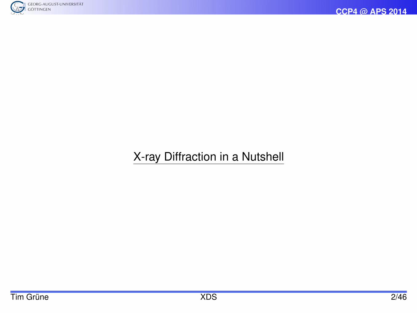
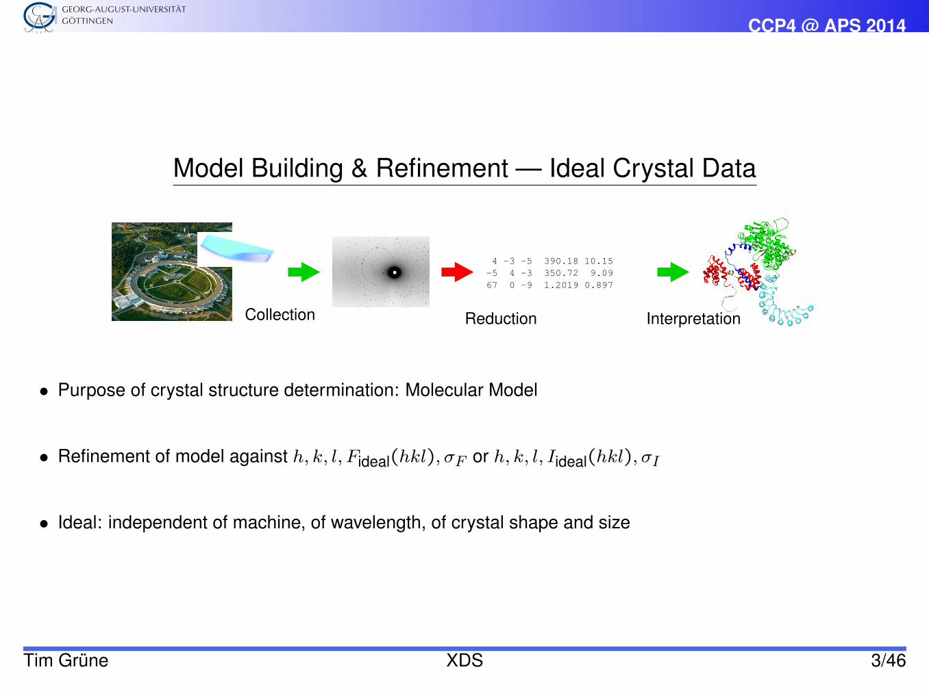
Model Building & Refinement — Ideal Crystal Data
4 −3 −5 390.18 10.15
−5 4 −3 350.72 9.09
67 0 −9 1.2019 0.897
Collection InterpretationReduction
• Purpose of crystal structure determination: Molecular Model
• Refinement of model against h, k, l, Fideal(hkl), σF or h, k, l, Iideal(hkl), σI
• Ideal: independent of machine, of wavelength, of crystal shape and size
Tim Grüne XDS 3/46
CCP4 @ APS 2014
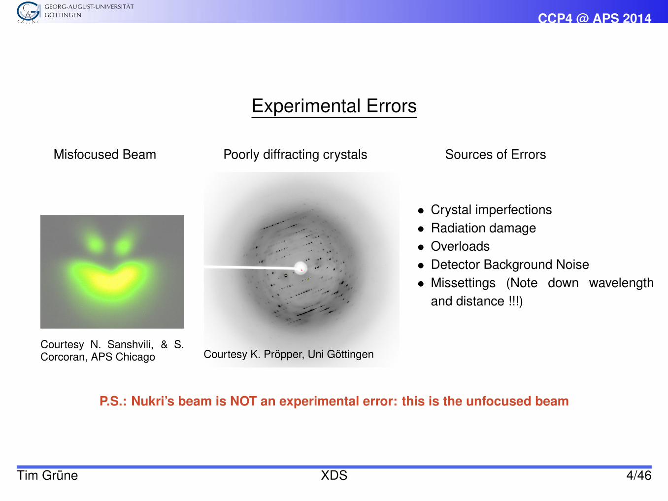
Experimental Errors
Misfocused Beam Poorly diffracting crystals Sources of Errors
• Crystal imperfections• Radiation damage• Overloads• Detector Background Noise• Missettings (Note down wavelength
and distance !!!)
Courtesy N. Sanshvili, & S.Corcoran, APS Chicago Courtesy K. Pröpper, Uni Göttingen
P.S.: Nukri’s beam is NOT an experimental error: this is the unfocused beam
Tim Grüne XDS 4/46
CCP4 @ APS 2014
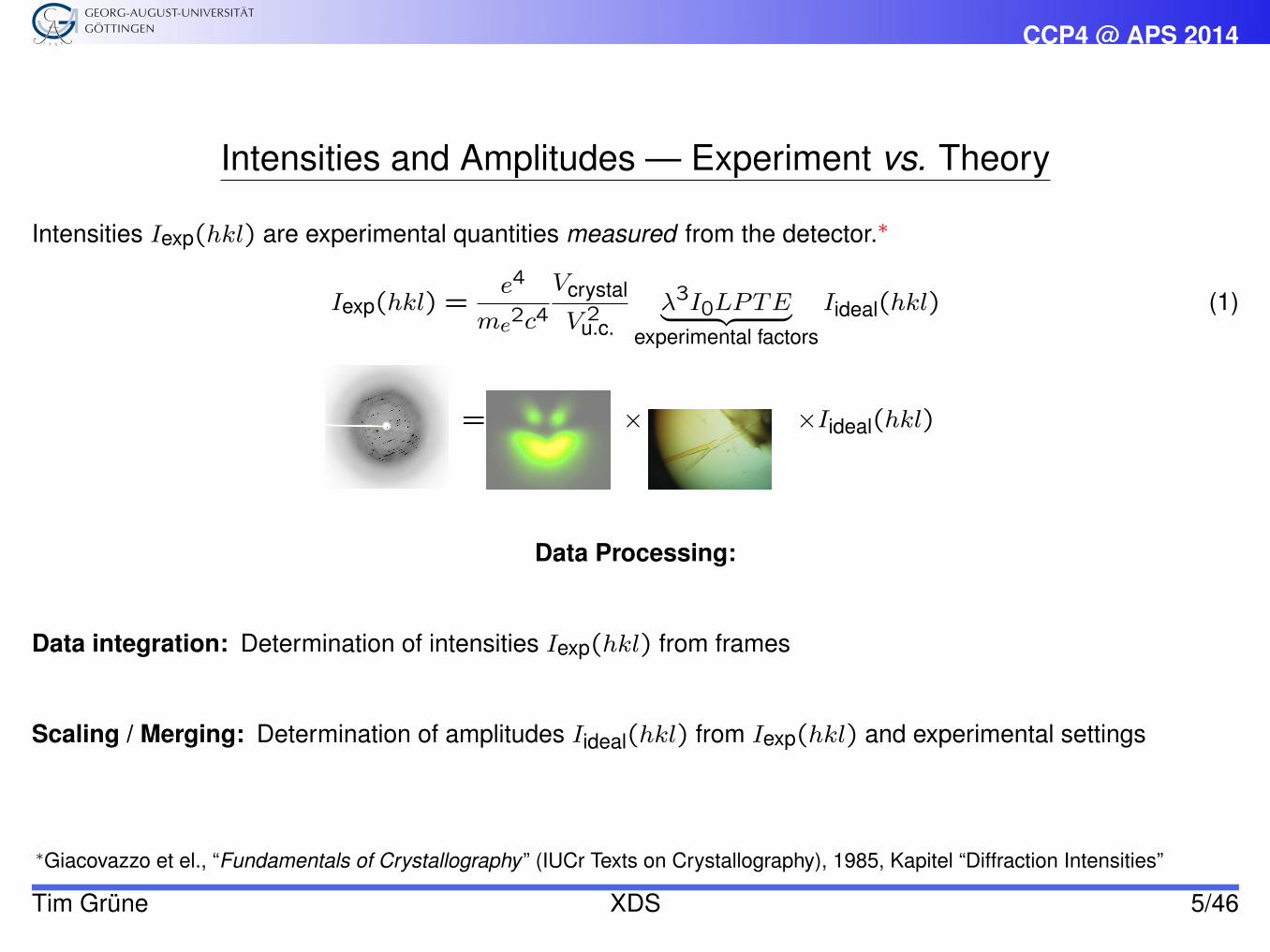
Intensities and Amplitudes — Experiment vs. Theory
Intensities Iexp(hkl) are experimental quantities measured from the detector.∗
Iexp(hkl) =e4
me2c4
Vcrystal
V 2u.c.
λ3I0LPTE︸ ︷︷ ︸experimental factors
Iideal(hkl) (1)
= × ×Iideal(hkl)
Data Processing:
Data integration: Determination of intensities Iexp(hkl) from frames
Scaling / Merging: Determination of amplitudes Iideal(hkl) from Iexp(hkl) and experimental settings
∗Giacovazzo et el., “Fundamentals of Crystallography ” (IUCr Texts on Crystallography), 1985, Kapitel “Diffraction Intensities”
Tim Grüne XDS 5/46
CCP4 @ APS 2014
Understanding your last Experiment
—The Ewald Sphere Construction
Tim Grüne XDS 6/46
CCP4 @ APS 2014
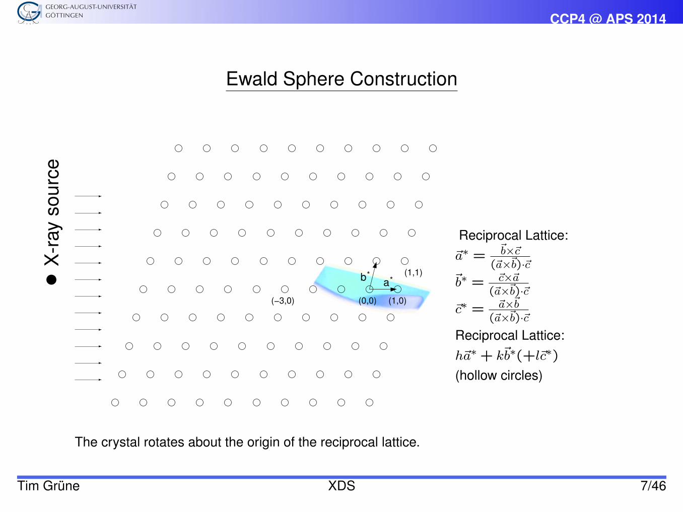
Ewald Sphere Construction
(1,0)
*
(−3,0)
b* (1,1)
a
(0,0)
~
-
-
-
-
-
-
-
-
-
-
-
-
X-r
ayso
urce
Reciprocal Lattice:~a∗ =
~b×~c(~a×~b)·~c
~b∗ = ~c×~a(~a×~b)·~c
~c∗ = ~a×~b(~a×~b)·~c
Reciprocal Lattice:h~a∗+ k~b∗(+l~c∗)
(hollow circles)
The crystal rotates about the origin of the reciprocal lattice.
Tim Grüne XDS 7/46
CCP4 @ APS 2014
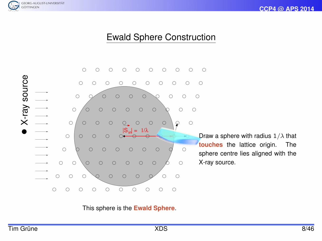
Ewald Sphere Construction
1/λ|S | =in~
-
-
-
-
-
-
-
-
-
-
-
-
X-r
ayso
urce
Draw a sphere with radius 1/λ thattouches the lattice origin. Thesphere centre lies aligned with theX-ray source.
This sphere is the Ewald Sphere.
Tim Grüne XDS 8/46
CCP4 @ APS 2014
Ewald Sphere Construction
S
|S in|
|S out |
(0, −2)
(−1, 2)
(−5, −3)
(−7, −1)
~
-
-
-
-
-
-
-
-
-
-
-
-
X-r
ayso
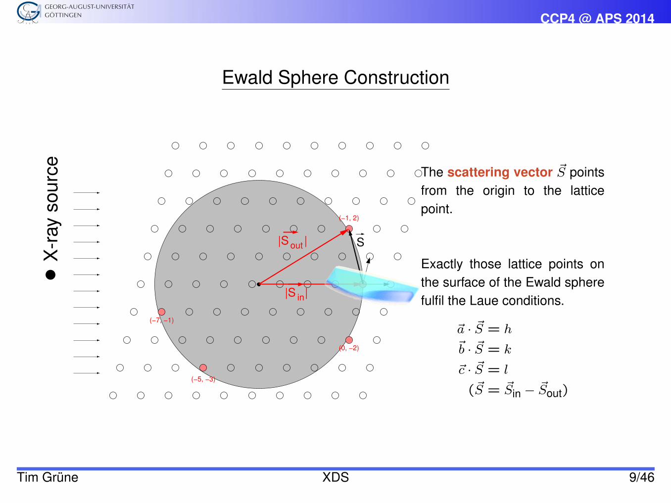
urce The scattering vector ~S points
from the origin to the latticepoint.
Exactly those lattice points onthe surface of the Ewald spherefulfil the Laue conditions.
~a · ~S = h
~b · ~S = k
~c · ~S = l
(~S = ~Sin − ~Sout)
Tim Grüne XDS 9/46
CCP4 @ APS 2014
Ewald Sphere Construction
(0, −2)
(−1, 2)
(−5, −3)
2θ′
(−7, −1)
(−1,2)
(0,0)
(0,−2)
Dete
cto
r
2θ
~
-
-
-
-
-
-
-
-
-
-
-
-
X-r
ayso
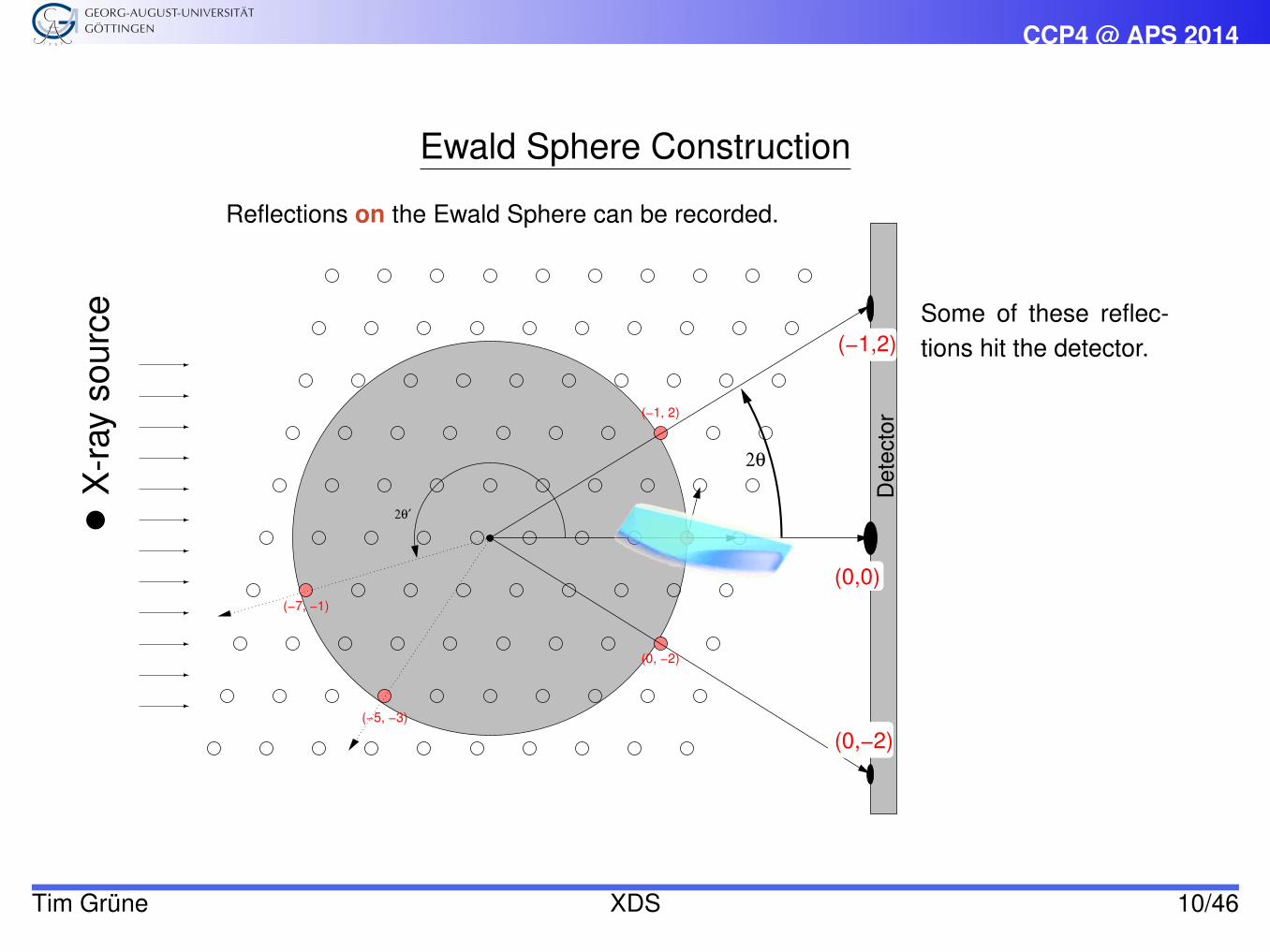
urce Some of these reflec-
tions hit the detector.
Reflections on the Ewald Sphere can be recorded.
Tim Grüne XDS 10/46
CCP4 @ APS 2014
Ewald Sphere Construction
Dete
cto
r
(0, 2)
~
-
-
-
-
-
-
-
-
-
-
-
-
X-r
ayso
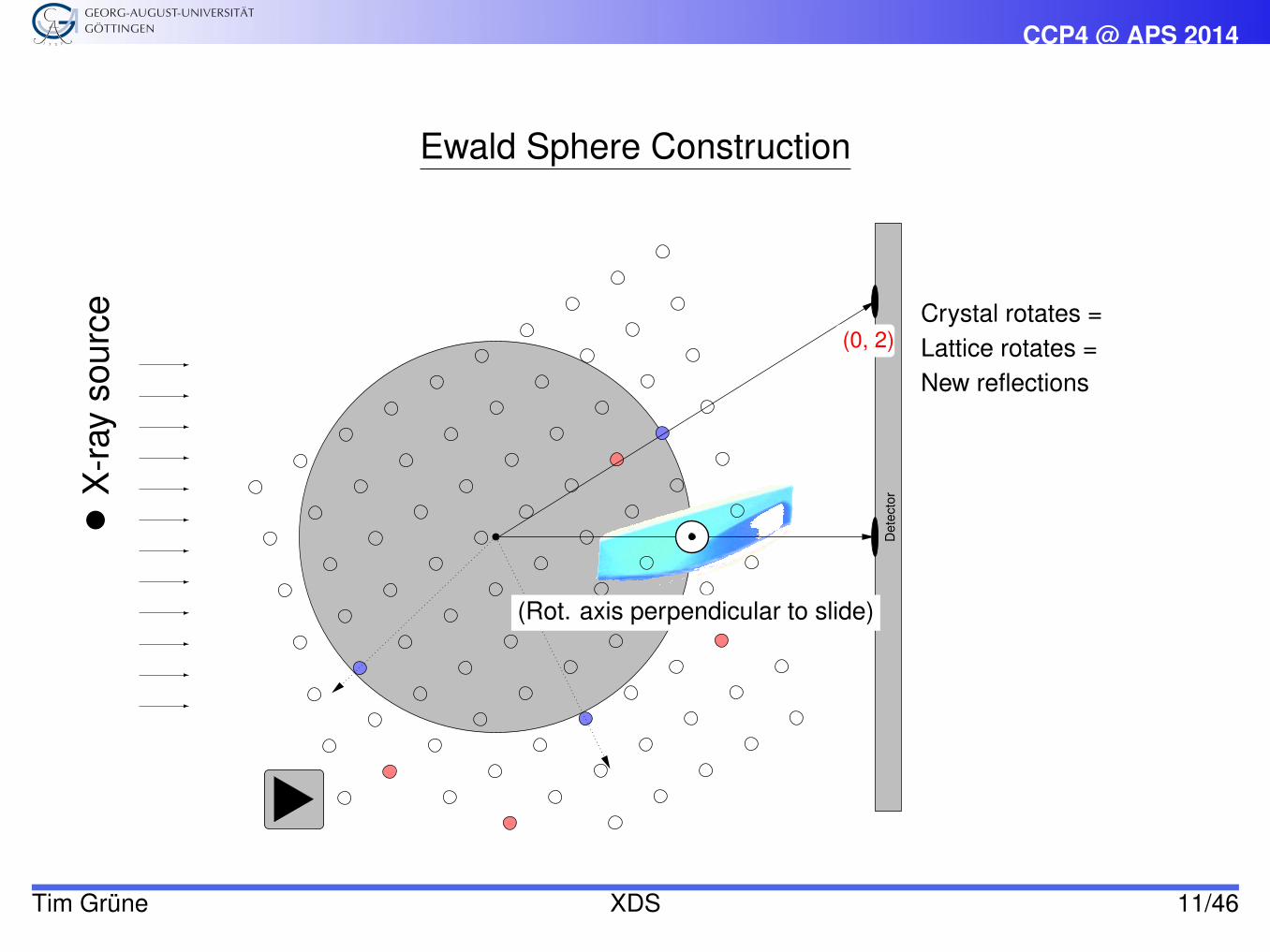
urce Crystal rotates =
Lattice rotates =New reflections
(Rot. axis perpendicular to slide)
Tim Grüne XDS 11/46
CCP4 @ APS 2014
Ewald Sphere Construction
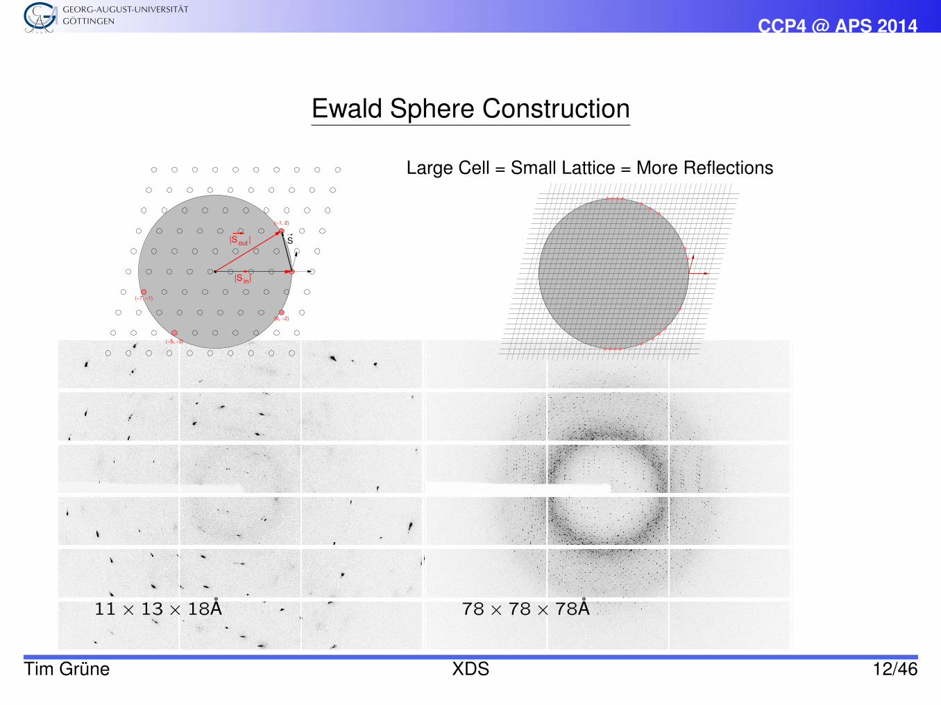
Large Cell = Small Lattice = More Reflections
S
|S in|
|S out |
(0, −2)
(−1, 2)
(−5, −3)
(−7, −1)
11× 13× 18Å 78× 78× 78Å
Tim Grüne XDS 12/46
CCP4 @ APS 2014
Example Application: Inverse Beam for Anomalous Phasing
1a
1b
2a
2b
3a
3b
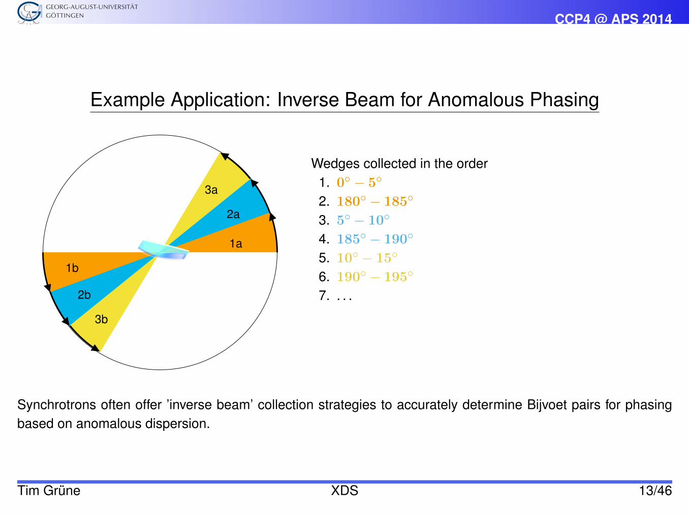
Wedges collected in the order1. 0◦ − 5◦
2. 180◦ − 185◦
3. 5◦ − 10◦
4. 185◦ − 190◦
5. 10◦ − 15◦
6. 190◦ − 195◦
7. . . .
Synchrotrons often offer ’inverse beam’ collection strategies to accurately determine Bijvoet pairs for phasingbased on anomalous dispersion.
Tim Grüne XDS 13/46
CCP4 @ APS 2014
Bijvoet Pairs and Inverse Beam
��������
��������
(−5, −3)
(−7, −1)
(−1,2)
(0,0)
(0,−2)D
ete
kto
r
(1, −2)
(0, 2)(−1, 2)
(0, −2) ��������
��������
��������
��������
(5, 3)
(7, 1)
(0,0)
(1,−2)
(0,2)
(0, −2)
(0, 2) (−1, 2)
(1, −2)
De
tekto
r
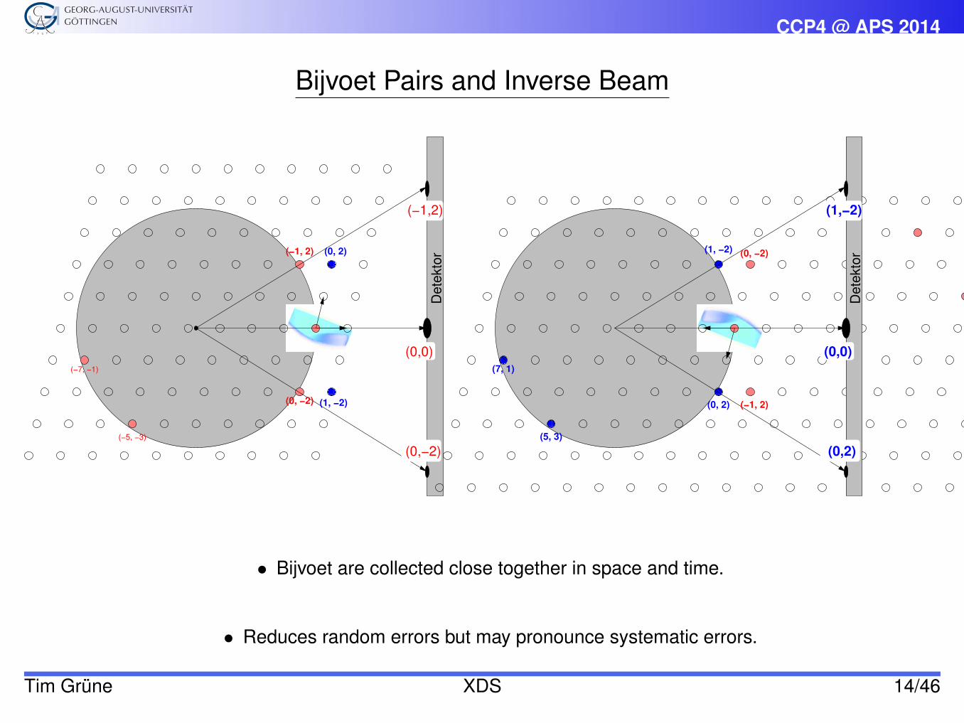
• Bijvoet are collected close together in space and time.
• Reduces random errors but may pronounce systematic errors.
Tim Grüne XDS 14/46
CCP4 @ APS 2014
Data Processing with XDS
Tim Grüne XDS 15/46
CCP4 @ APS 2014
Data Processing
Processing your Data = Getting Iideal from you experiment
Understanding your Reduction Program(s) = Getting the best Iideal from you experiment
Tim Grüne XDS 16/46
CCP4 @ APS 2014
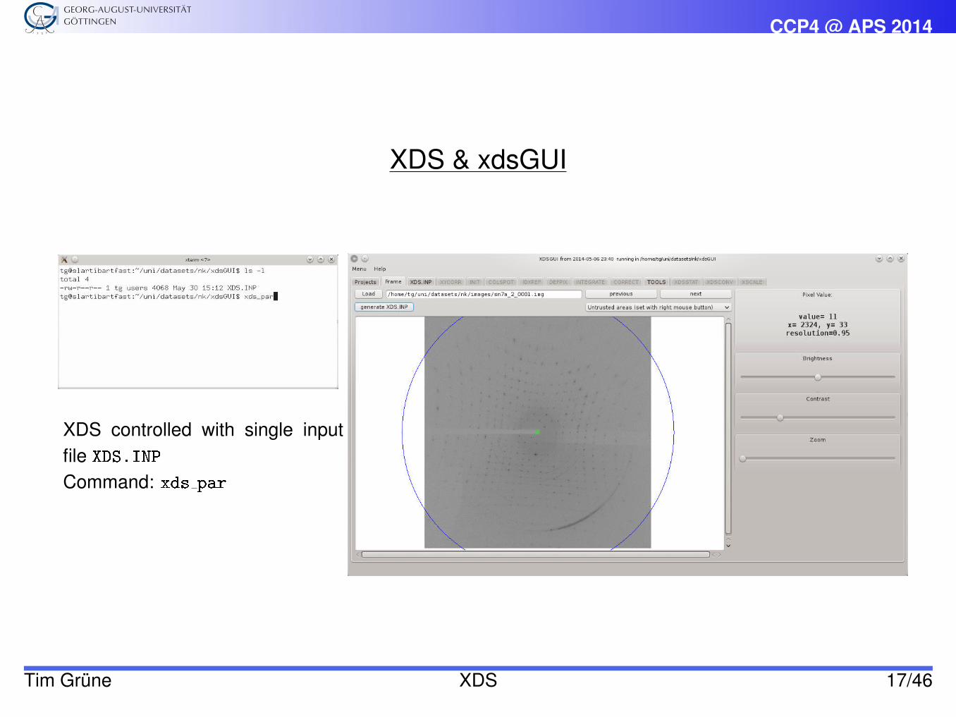
XDS & xdsGUI
XDS controlled with single inputfile XDS.INP
Command: xds par
Tim Grüne XDS 17/46
CCP4 @ APS 2014
XDS.INP
XDS is controlled by one single input file: XDS.INP.
• Name cannot be changed• Each data set must be run in separate directory to avoid overwriting of files.• Contains about 100 Keywords a of the form
KEYWORD=VALUE
• Only about 10 Keywords must be modified for most data sets (e.g. image names, detectordistance, number of images, etc.)• Most important one:
JOB= XYCORR INIT COLSPOT IDXREF DEFPIX INTEGRATE CORRECT
Each name stands for one of the steps XDS carries out during data integration.aalso called “cards” for historical reasons
Tim Grüne XDS 18/46
CCP4 @ APS 2014
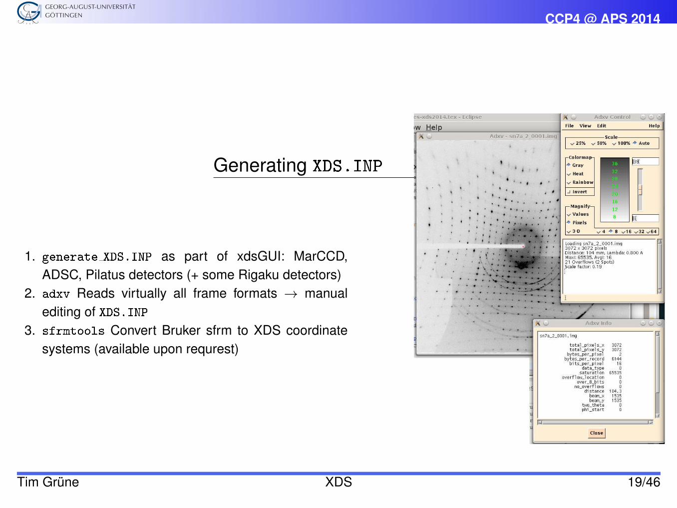
Generating XDS.INP
1. generate XDS.INP as part of xdsGUI: MarCCD,ADSC, Pilatus detectors (+ some Rigaku detectors)
2. adxv Reads virtually all frame formats → manualediting of XDS.INP
3. sfrmtools Convert Bruker sfrm to XDS coordinatesystems (available upon requrest)
Tim Grüne XDS 19/46
CCP4 @ APS 2014
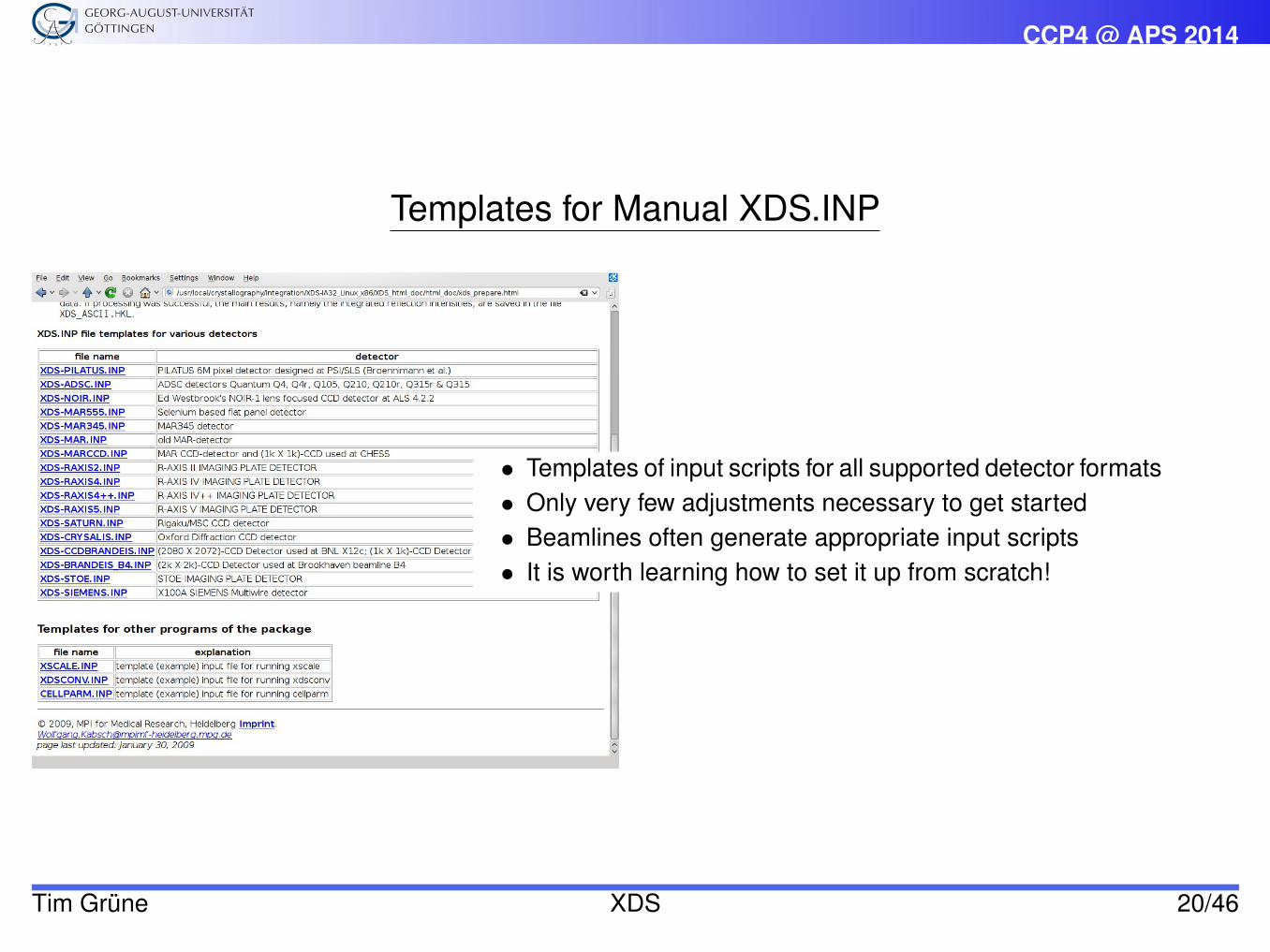
Templates for Manual XDS.INP
• Templates of input scripts for all supported detector formats• Only very few adjustments necessary to get started• Beamlines often generate appropriate input scripts• It is worth learning how to set it up from scratch!
Tim Grüne XDS 20/46
CCP4 @ APS 2014
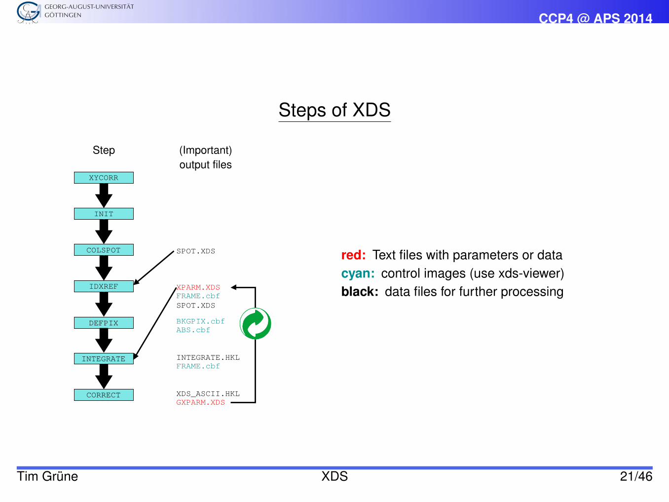
Steps of XDS
IDXREF
COLSPOT
INIT
XYCORR
CORRECT
INTEGRATE
DEFPIX
XPARM.XDS
INTEGRATE.HKL
XDS_ASCII.HKL
GXPARM.XDS
BKGPIX.cbf
ABS.cbf
FRAME.cbf
FRAME.cbf
Step (Important)
output files
SPOT.XDS
SPOT.XDS
red: Text files with parameters or datacyan: control images (use xds-viewer)black: data files for further processing
Tim Grüne XDS 21/46
CCP4 @ APS 2014
The Steps
XYINIT writes files for positional corrections of the detector plane. Most modern detectors providealready corrected images so that these to files are normally flat.
INIT determines initial detector backgroundCOLSPOT Strong reflections for indexingIDXREF indexing: unit cell dimensions and crystal orientationDEFPIX set active dectector area (exclude resolution cut-off, beam stop shadow, . . . )INTEGRATE extract reflection intensities from frames→ Iexp(hkl)CORRECT applies corrections (polarisation, Lorentz-correction, . . . ), scales reflections, reports data
statistics→ Iideal(hkl)
Tim Grüne XDS 22/46
CCP4 @ APS 2014
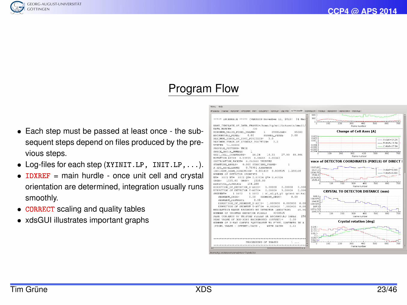
Program Flow
• Each step must be passed at least once - the sub-sequent steps depend on files produced by the pre-vious steps.• Log-files for each step (XYINIT.LP, INIT.LP,...).• IDXREF = main hurdle - once unit cell and crystal
orientation are determined, integration usually runssmoothly.• CORRECT scaling and quality tables• xdsGUI illustrates important graphs
Tim Grüne XDS 23/46
CCP4 @ APS 2014
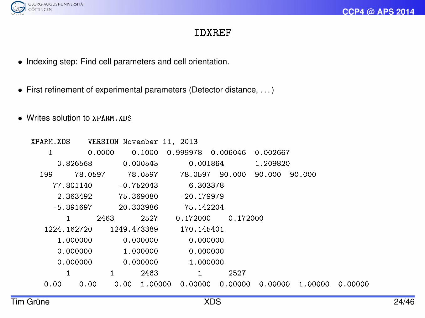
IDXREF
• Indexing step: Find cell parameters and cell orientation.
• First refinement of experimental parameters (Detector distance, . . . )
• Writes solution to XPARM.XDS
XPARM.XDS VERSION November 11, 2013
1 0.0000 0.1000 0.999978 0.006046 0.002667
0.826568 0.000543 0.001864 1.209820
199 78.0597 78.0597 78.0597 90.000 90.000 90.000
77.801140 -0.752043 6.303378
2.363492 75.369080 -20.179979
-5.891697 20.303986 75.142204
1 2463 2527 0.172000 0.172000
1224.162720 1249.473389 170.145401
1.000000 0.000000 0.000000
0.000000 1.000000 0.000000
0.000000 0.000000 1.000000
1 1 2463 1 2527
0.00 0.00 0.00 1.00000 0.00000 0.00000 0.00000 1.00000 0.00000
Tim Grüne XDS 24/46
CCP4 @ APS 2014
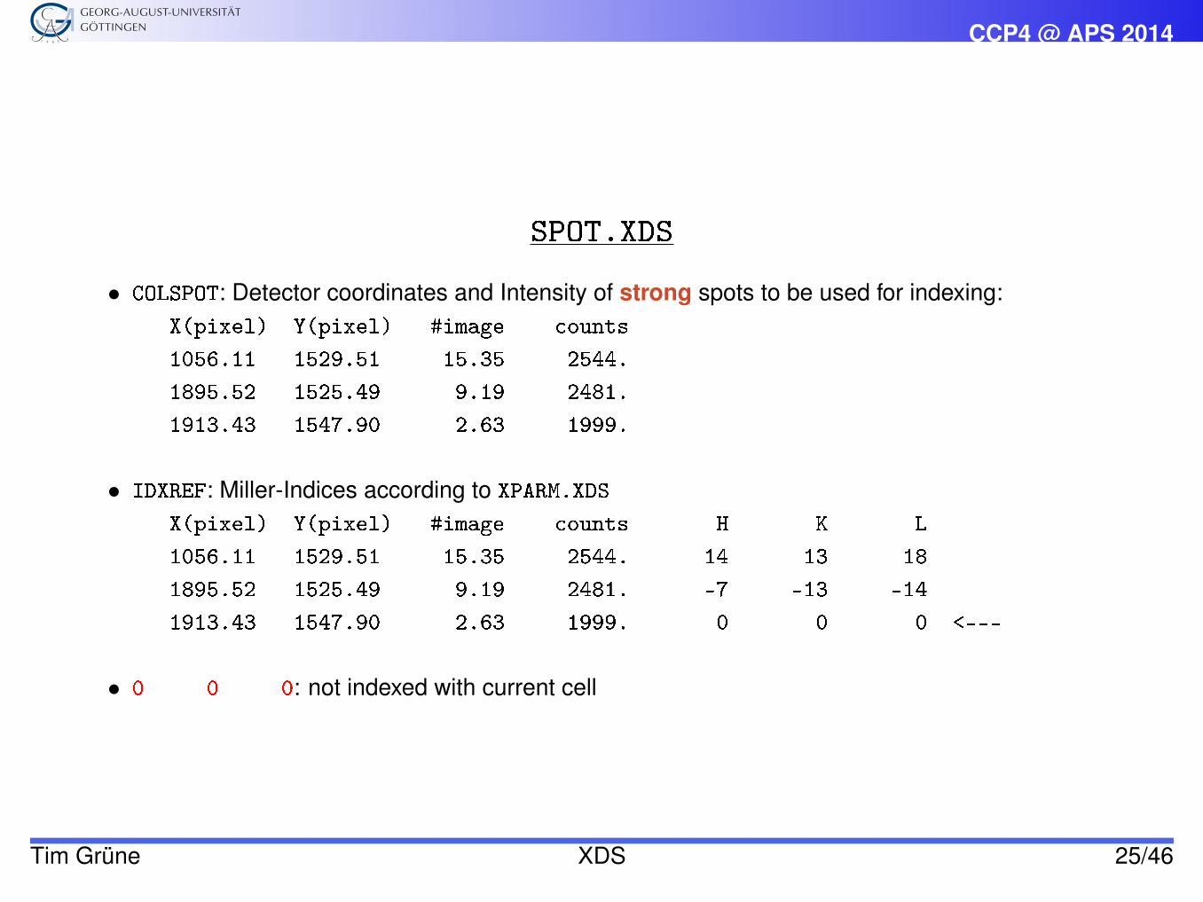
SPOT.XDS
• COLSPOT: Detector coordinates and Intensity of strong spots to be used for indexing:X(pixel) Y(pixel) #image counts
1056.11 1529.51 15.35 2544.
1895.52 1525.49 9.19 2481.
1913.43 1547.90 2.63 1999.
• IDXREF: Miller-Indices according to XPARM.XDS
X(pixel) Y(pixel) #image counts H K L
1056.11 1529.51 15.35 2544. 14 13 18
1895.52 1525.49 9.19 2481. -7 -13 -14
1913.43 1547.90 2.63 1999. 0 0 0 <---
• 0 0 0: not indexed with current cell
Tim Grüne XDS 25/46
CCP4 @ APS 2014
“!!! ERROR !!! SOLUTION IS INACCURATE”
Correct indexing is crucial for data integration. If XDS indexes 50 % of all spots in SPOT.XDS it stops with theabove error message.
Most common reasons:
1. Wrong ORGX, ORGY2. Wrong Parameter settings (Detector distance, wavelength)3. Poor data quality
Tim Grüne XDS 26/46
CCP4 @ APS 2014
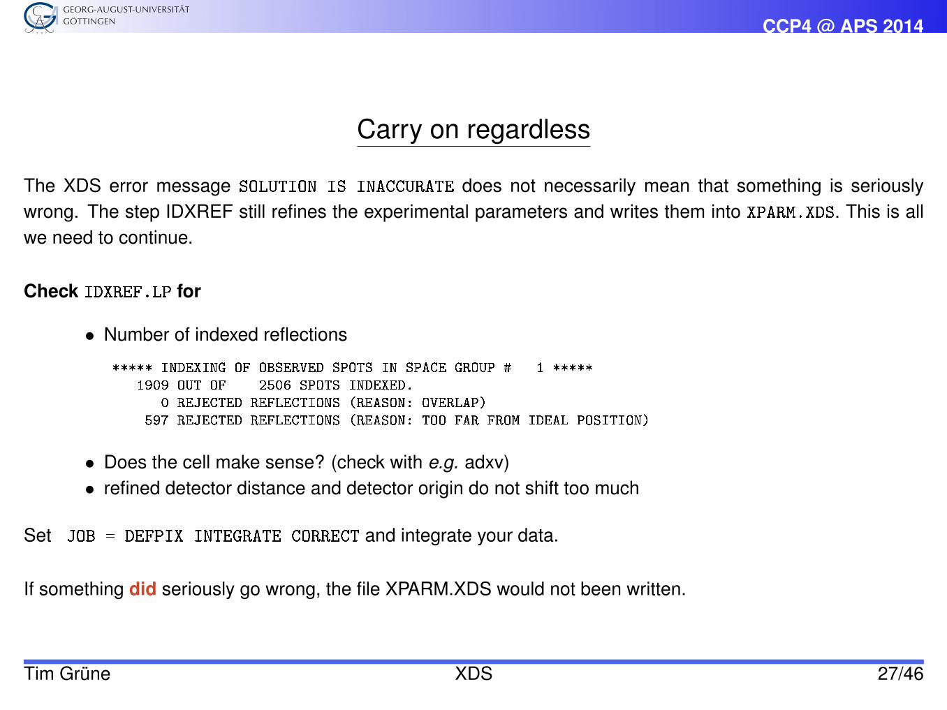
Carry on regardless
The XDS error message SOLUTION IS INACCURATE does not necessarily mean that something is seriouslywrong. The step IDXREF still refines the experimental parameters and writes them into XPARM.XDS. This is allwe need to continue.
Check IDXREF.LP for
• Number of indexed reflections
***** INDEXING OF OBSERVED SPOTS IN SPACE GROUP # 1 *****
1909 OUT OF 2506 SPOTS INDEXED.
0 REJECTED REFLECTIONS (REASON: OVERLAP)
597 REJECTED REFLECTIONS (REASON: TOO FAR FROM IDEAL POSITION)
• Does the cell make sense? (check with e.g. adxv)• refined detector distance and detector origin do not shift too much
Set JOB = DEFPIX INTEGRATE CORRECT and integrate your data.
If something did seriously go wrong, the file XPARM.XDS would not been written.
Tim Grüne XDS 27/46
CCP4 @ APS 2014
DEFPIX: active detector mask
DEFPIX sets the area of the detector which is taken into account during integration. It takes into account:
1. INCLUDE_RESOLUTION_RANGE default: 20 Å to detector edge.2. VALUE_RANGE_FOR_TRUSTED_DETECTOR_PIXELS exclude shadowed regions, e.g. beamstop, cryo
stream nozzle3. UNTRUSTED_RECTANGLE exclude gaps of CCD chips e.g. Pilatus detector (automatic)4. EXCLUDE_RESOLUTION_RANGE exclude ice rings from data integration
Tim Grüne XDS 28/46
CCP4 @ APS 2014
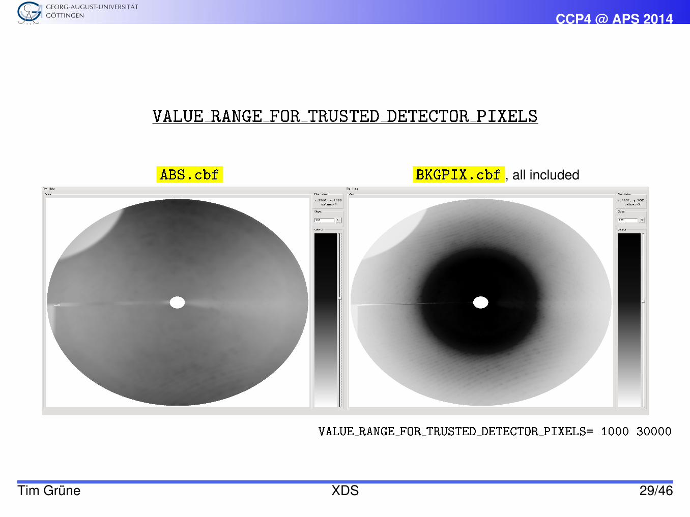
VALUE RANGE FOR TRUSTED DETECTOR PIXELS
ABS.cbf BKGPIX.cbf , all included
VALUE RANGE FOR TRUSTED DETECTOR PIXELS= 1000 30000
Tim Grüne XDS 29/46

CCP4 @ APS 2014
VALUE RANGE FOR TRUSTED DETECTOR PIXELS
ABS.cbf BKGPIX.cbf , shadows removed
VALUE RANGE FOR TRUSTED DETECTOR PIXELS= 6100 30000
Tim Grüne XDS 30/46
CCP4 @ APS 2014
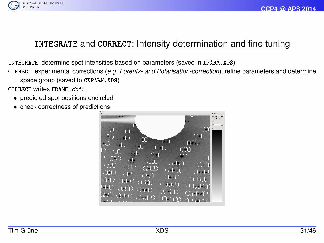
INTEGRATE and CORRECT: Intensity determination and fine tuning
INTEGRATE determine spot intensities based on parameters (saved in XPARM.XDS)CORRECT experimental corrections (e.g. Lorentz- and Polarisation-correction), refine parameters and determine
space group (saved to GXPARM.XDS)CORRECT writes FRAME.cbf:• predicted spot positions encircled• check correctness of predictions
Tim Grüne XDS 31/46
CCP4 @ APS 2014
Recycling
• Parameters (in GXPARM.XDS) depend on measured intensities• Intensities (including corrections) depend on Parameters⇒ rename GXPARM.XDS to XPARM.XDS and rerun XDS (JOB = DEFPIX INTEGRATE CORRECT) to im-
prove results.
This way one should also set the correct high- and low- resolution cut-offs
Tim Grüne XDS 32/46
CCP4 @ APS 2014
Resolution Cut-Off
The default resolution range in XDS is 20 Å to the detector edge
INCLUDE_RESOLUTION_RANGE=20.0 0.0
• Medium to low resolution data: increase 20 Å to 30 Å or even 50 Å (check BKGPIX.cbf)• After second round of integration: determine high-resolution cut-off.
Why after second round?
• Correct space group rather than P1
⇒ more symmetry related reflections⇒ more reliable data statistics, especially I/σI
Tim Grüne XDS 33/46
CCP4 @ APS 2014
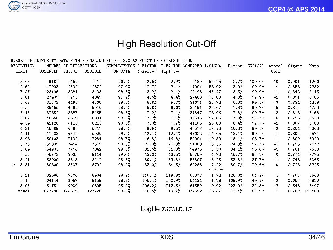
High Resolution Cut-Off
SUBSET OF INTENSITY DATA WITH SIGNAL/NOISE >= -3.0 AS FUNCTION OF RESOLUTIONRESOLUTION NUMBER OF REFLECTIONS COMPLETENESS R-FACTOR R-FACTOR COMPARED I/SIGMA R-meas CC(1/2) Anomal SigAno Nano
LIMIT OBSERVED UNIQUE POSSIBLE OF DATA observed expected Corr
13.63 9181 1459 1511 96.6% 2.5% 2.9% 9180 55.25 2.7% 100.0* 10 0.901 12069.64 17093 2592 2672 97.0% 2.7% 3.1% 17091 53.02 3.0% 99.9* 4 0.858 23327.87 23196 3381 3433 98.5% 3.2% 3.4% 23195 46.27 3.5% 99.9* -1 0.848 31156.81 27489 3965 4049 97.9% 4.5% 4.4% 27483 35.88 4.8% 99.9* -2 0.851 37056.09 31672 4498 4565 98.5% 5.8% 5.7% 31671 28.72 6.3% 99.8* -3 0.834 42585.56 35456 4969 5040 98.6% 6.8% 6.6% 35451 25.07 7.3% 99.7* -5 0.816 47525.15 37852 5387 5465 98.6% 7.2% 7.1% 37847 23.06 7.8% 99.7* -3 0.818 51684.82 40555 5829 5894 98.9% 7.2% 7.1% 40546 22.85 7.8% 99.7* -5 0.795 55494.54 41126 6125 6213 98.6% 7.8% 7.7% 41105 20.88 8.4% 99.7* -2 0.807 57884.31 45588 6568 6647 98.8% 9.5% 9.5% 45578 17.93 10.3% 99.5* -2 0.804 63024.11 47633 6842 6900 99.2% 12.4% 12.4% 47622 14.05 13.4% 99.2* -1 0.805 65743.93 50103 7192 7284 98.7% 16.8% 16.8% 50091 10.89 18.1% 98.7* -1 0.800 69403.78 51899 7414 7519 98.6% 23.0% 22.9% 51889 8.35 24.9% 97.7* -1 0.796 71723.64 54983 7766 7842 99.0% 31.6% 31.8% 54975 6.30 34.1% 96.0* -1 0.781 75333.52 56772 8033 8114 99.0% 43.3% 43.5% 56759 4.72 46.7% 93.2* 0 0.774 77853.41 58909 8313 8412 98.8% 59.1% 59.8% 58897 3.45 63.8% 87.7* -1 0.748 8065
--> 3.31 60300 8607 8702 98.9% 83.0% 84.5% 60285 2.42 89.7% 79.6* 0 0.728 8345^^^^^^
3.21 62086 8804 8904 98.9% 116.7% 119.8% 62073 1.72 126.0% 64.9* 1 0.705 85633.13 64144 9057 9159 98.9% 156.4% 160.9% 64134 1.28 168.9% 49.9* -2 0.666 88203.05 61751 9009 9395 95.9% 206.2% 212.5% 61650 0.92 223.0% 34.5* -2 0.643 8497
total 877788 125810 127720 98.5% 10.5% 10.7% 877522 13.37 11.4% 99.9* -1 0.769 120469
Logfile XSCALE.LP
Tim Grüne XDS 34/46
CCP4 @ APS 2014
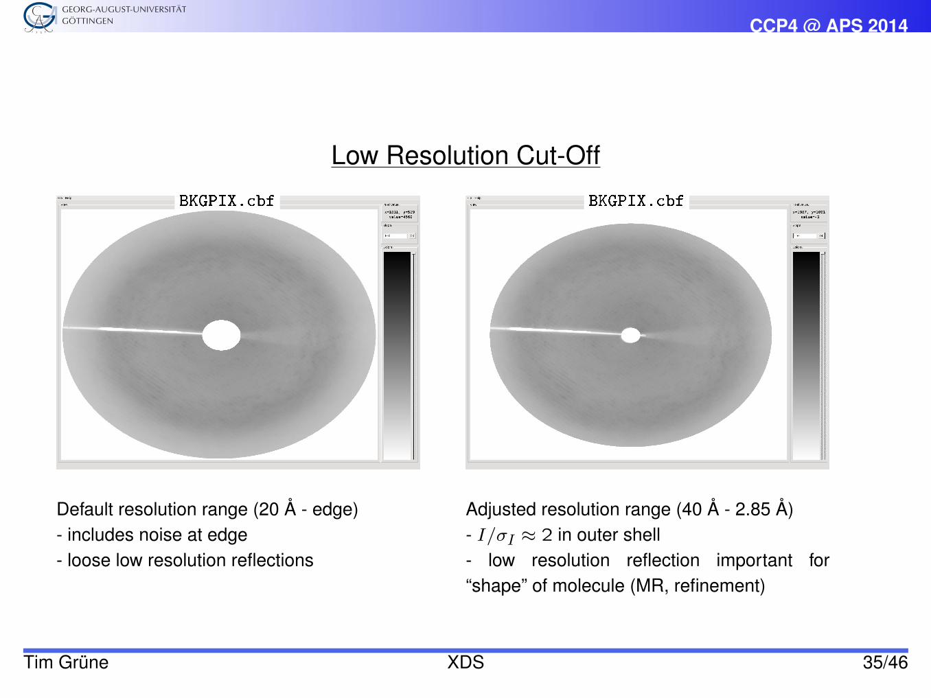
Low Resolution Cut-Off
BKGPIX.cbf BKGPIX.cbf
Default resolution range (20 Å - edge)- includes noise at edge- loose low resolution reflections
Adjusted resolution range (40 Å - 2.85 Å)- I/σI ≈ 2 in outer shell- low resolution reflection important for“shape” of molecule (MR, refinement)
Tim Grüne XDS 35/46
CCP4 @ APS 2014
XDS and Friedel’s Law
• XDS.INP and XSCALE.INP allow the keyword FRIEDEL'S LAW=FALSE
• Frequent belief: ’TRUE’ = merging of Bijvoet pairs = loss of anomalous signal
• Correct:
– XDS ASCII.HKL always unmerged
– FRIEDEL'S LAW=TRUE only affects scaling and statistics
• FRIEDEL'S LAW=TRUE: twice as many reflections
– more reliable statistics
– better anomalous signal
Tim Grüne XDS 36/46
CCP4 @ APS 2014
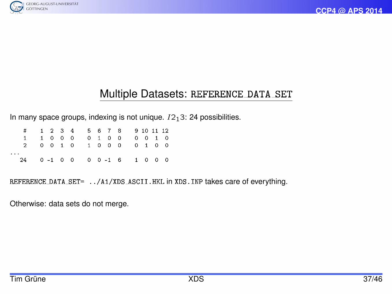
Multiple Datasets: REFERENCE DATA SET
In many space groups, indexing is not unique. I213: 24 possibilities.
# 1 2 3 4 5 6 7 8 9 10 11 12
1 1 0 0 0 0 1 0 0 0 0 1 0
2 0 0 1 0 1 0 0 0 0 1 0 0
...
24 0 -1 0 0 0 0 -1 6 1 0 0 0
REFERENCE DATA SET= ../A1/XDS ASCII.HKL in XDS.INP takes care of everything.
Otherwise: data sets do not merge.
Tim Grüne XDS 37/46
CCP4 @ APS 2014
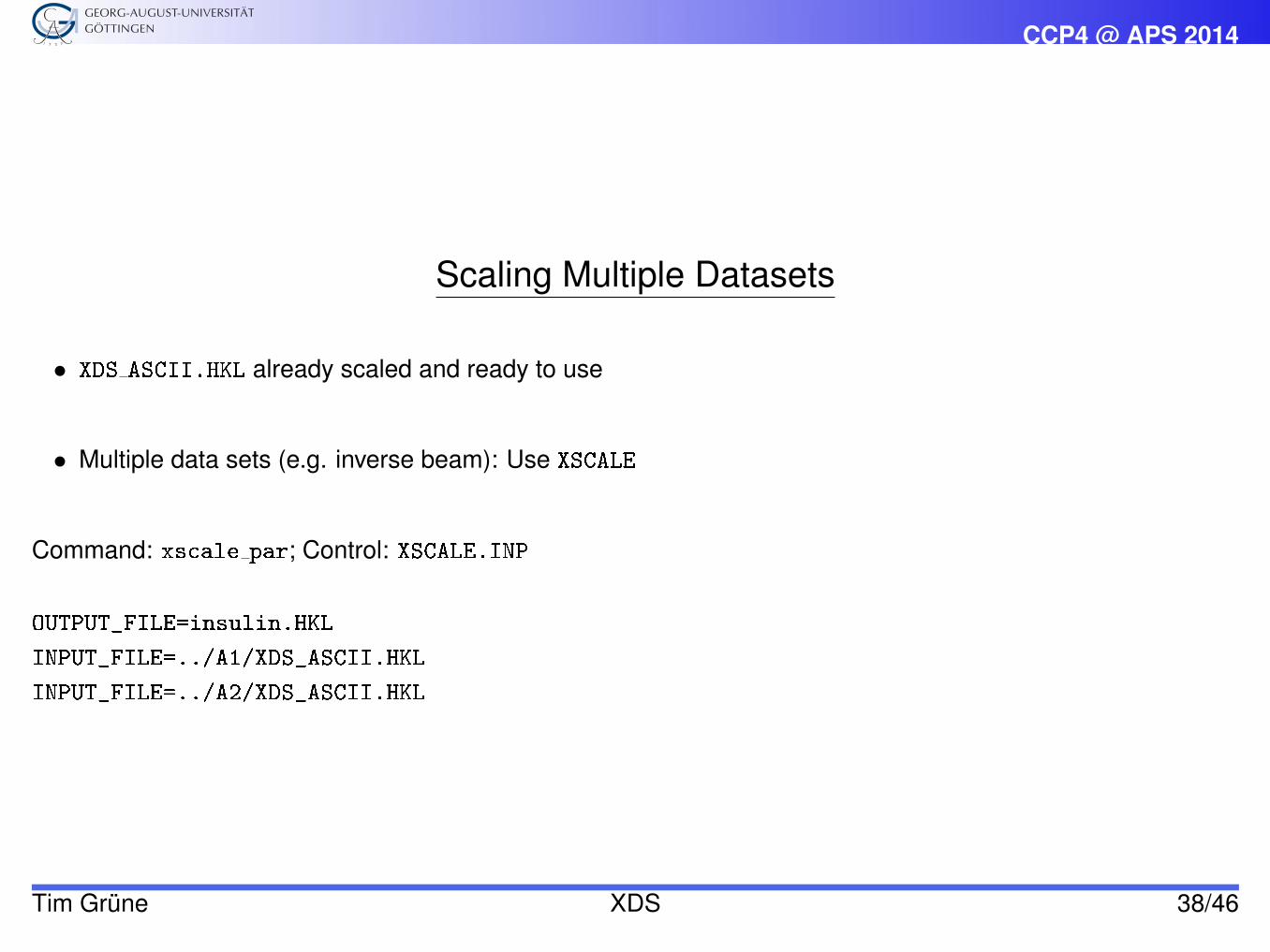
Scaling Multiple Datasets
• XDS ASCII.HKL already scaled and ready to use
• Multiple data sets (e.g. inverse beam): Use XSCALE
Command: xscale par; Control: XSCALE.INP
OUTPUT_FILE=insulin.HKL
INPUT_FILE=../A1/XDS_ASCII.HKL
INPUT_FILE=../A2/XDS_ASCII.HKL
Tim Grüne XDS 38/46
CCP4 @ APS 2014
Format Conversion
The final integrated data are written to the file XDS ASCII.HKL for each run.
1. for phasing with shelx c/d/e
2. for refinement (mtz-file)
Tim Grüne XDS 39/46
CCP4 @ APS 2014
Phasing with shelx c/d/e: HKL→ hkl
1. Phasing with shelx c/d/e requires no conversion
2. shelxc and xprep both read XDS and XSCALE output (HKL–) files
3. format detected automatically
Tim Grüne XDS 40/46
CCP4 @ APS 2014
HKL→ mtz
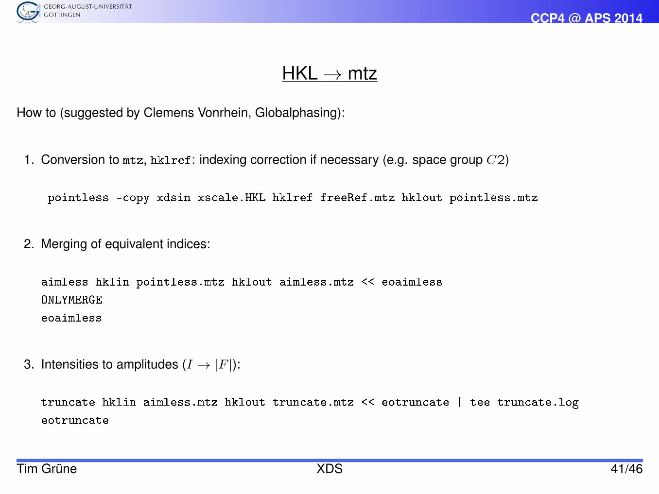
How to (suggested by Clemens Vonrhein, Globalphasing):
1. Conversion to mtz, hklref: indexing correction if necessary (e.g. space group C2)
pointless -copy xdsin xscale.HKL hklref freeRef.mtz hklout pointless.mtz
2. Merging of equivalent indices:
aimless hklin pointless.mtz hklout aimless.mtz << eoaimless
ONLYMERGE
eoaimless
3. Intensities to amplitudes (I → |F |):
truncate hklin aimless.mtz hklout truncate.mtz << eotruncate | tee truncate.log
eotruncate
Tim Grüne XDS 41/46
CCP4 @ APS 2014
HKL→ mtz (continued)
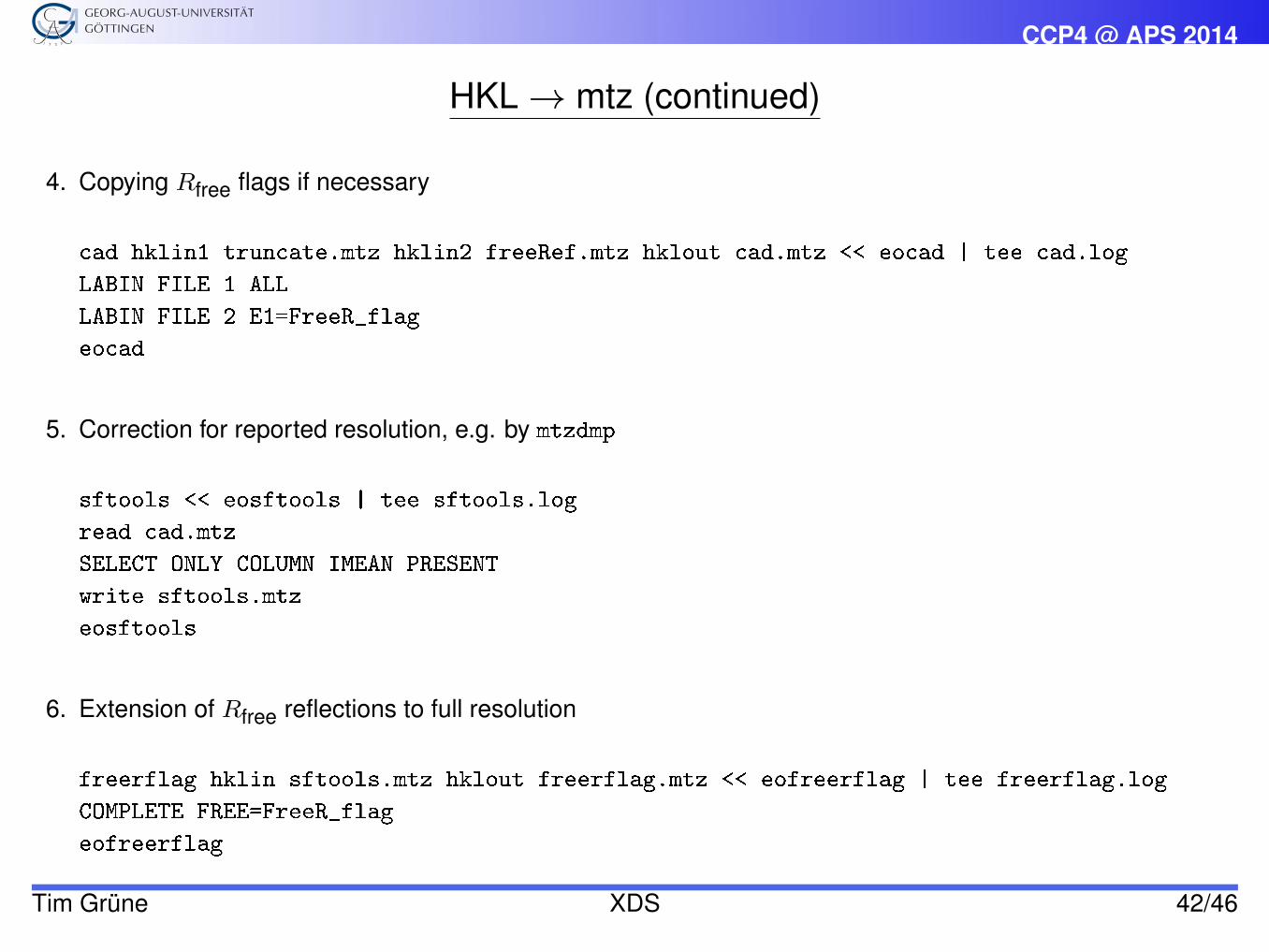
4. Copying Rfree flags if necessary
cad hklin1 truncate.mtz hklin2 freeRef.mtz hklout cad.mtz << eocad | tee cad.log
LABIN FILE 1 ALL
LABIN FILE 2 E1=FreeR_flag
eocad
5. Correction for reported resolution, e.g. by mtzdmp
sftools << eosftools | tee sftools.log
read cad.mtz
SELECT ONLY COLUMN IMEAN PRESENT
write sftools.mtz
eosftools
6. Extension of Rfree reflections to full resolution
freerflag hklin sftools.mtz hklout freerflag.mtz << eofreerflag | tee freerflag.log
COMPLETE FREE=FreeR_flag
eofreerflag
Tim Grüne XDS 42/46
CCP4 @ APS 2014
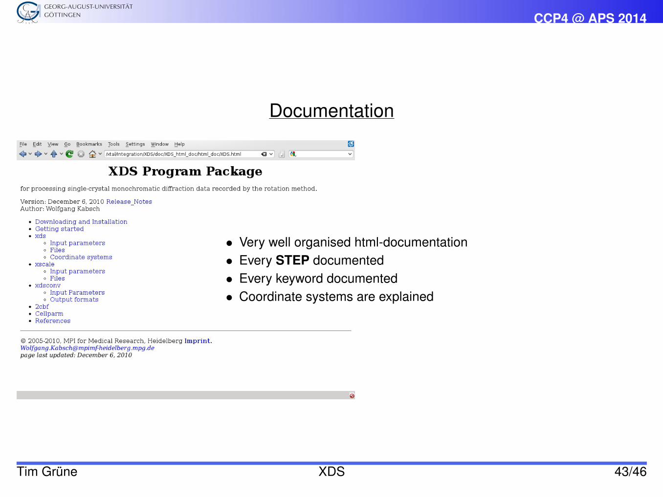
Documentation
• Very well organised html-documentation• Every STEP documented• Every keyword documented• Coordinate systems are explained
Tim Grüne XDS 43/46
CCP4 @ APS 2014
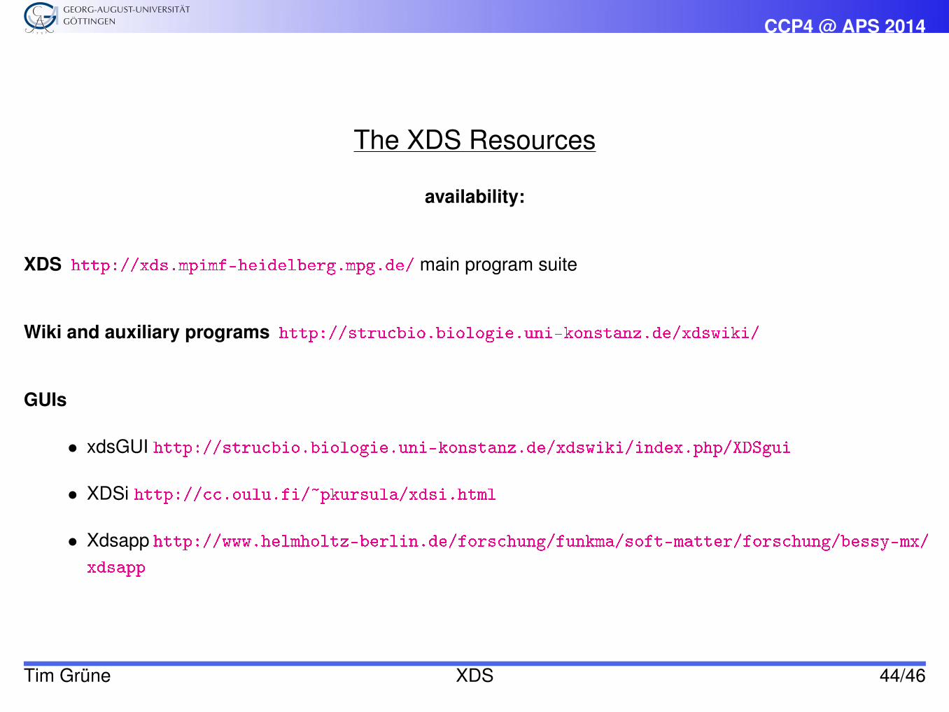
The XDS Resources
availability:
XDS http://xds.mpimf-heidelberg.mpg.de/ main program suite
Wiki and auxiliary programs http://strucbio.biologie.uni-konstanz.de/xdswiki/
GUIs
• xdsGUI http://strucbio.biologie.uni-konstanz.de/xdswiki/index.php/XDSgui
• XDSi http://cc.oulu.fi/~pkursula/xdsi.html
• Xdsapp http://www.helmholtz-berlin.de/forschung/funkma/soft-matter/forschung/bessy-mx/
xdsapp
Tim Grüne XDS 44/46
CCP4 @ APS 2014
References
XDS W. Kabsch, Acta Crystallogr. D66 (2010), 125–132
xdsGUI W. Brehm, K. Diederichs, M. Hoffer ( c©2013)
ADXV Andrew Arvai, http://www.scripps.edu/~arvai/adxv.html
MOSFLM H. R. Powell, O. Johnson and A. G. W. Leslie, Acta Crystallogr. D69 (2013), 1195-1203
CCP4 (pointless, aimless, . . . ) M. D. Winn et al., Acta Crystallogr. D67 (2011), 235–242
Tim Grüne XDS 45/46
CCP4 @ APS 2014
Acknowledgment
Lisandro Otero, Fundación Instituto Leloir, Argentina
Tim Grüne XDS 46/46