Embed Size (px)
Citation preview
Causality in
Quantum Theory
Katja Ried, Univ. InnsbruckSolstice of Foundations — ETH Zurich, June 2017
responsibility
free will
paradox
superposition ofcausal relations
purpose
statistical analysis
inference
epistemology
spacetime
relativitydeterminismknowledge vs reality
evidence-based policy
hidden variables
signalling
computational advantage
experiment indefinite causal order
quantum gravity
1.Causality (classical version)
● concepts and formalism
● features and phenomena
2.Quantum indeterminism
3.Retrocausality and causal loops
4.Nonlocality
● in quantum field theory
● Bell inequality violations
5.Quantum causal models
● concepts and formalism
6.Causal structure (quantum version)
● non-classical causal relations
● experiments
Itinerary
Causality(classical version)
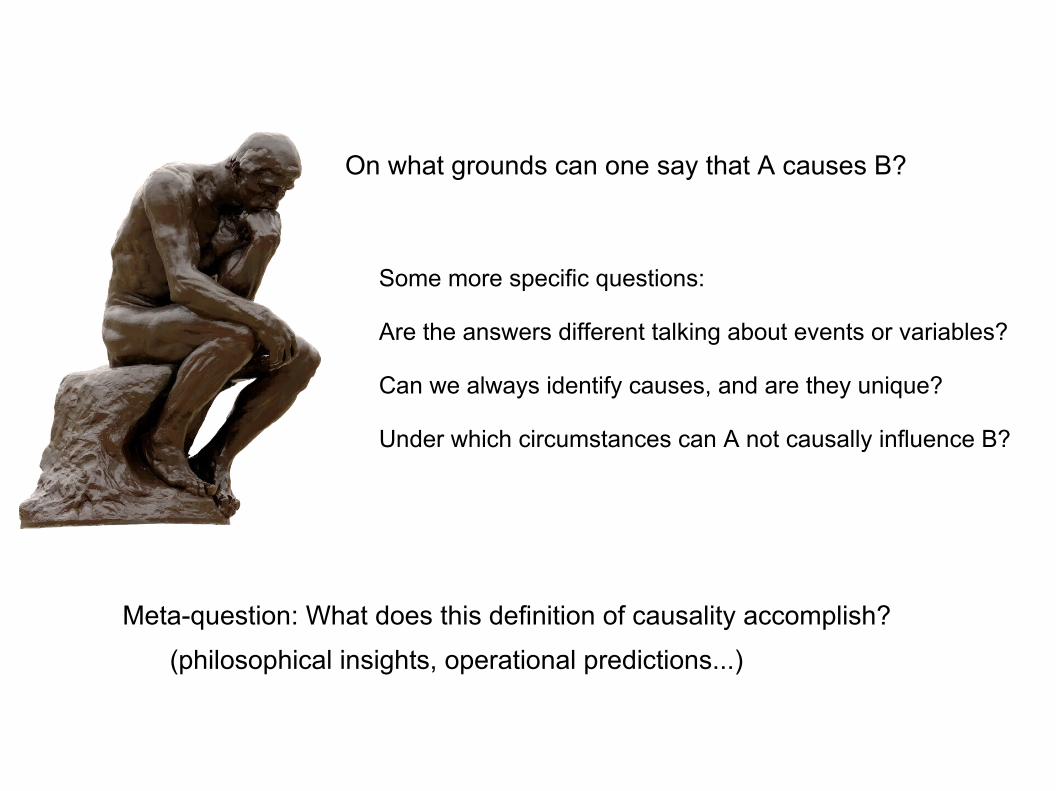
On what grounds can one say that A causes B?
Some more specific questions:
Are the answers different talking about events or variables?
Can we always identify causes, and are they unique?
Under which circumstances can A not causally influence B?
Meta-question: What does this definition of causality accomplish?
(philosophical insights, operational predictions...)
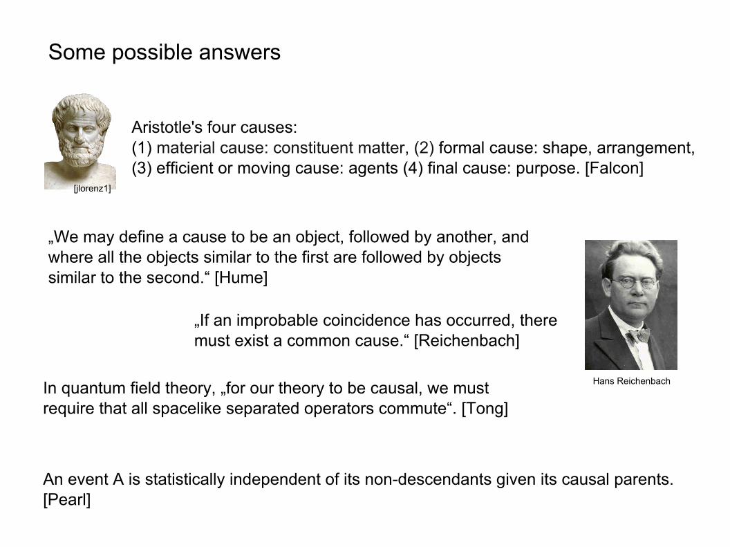
Some possible answers
Aristotle's four causes: (1) material cause: constituent matter, (2) formal cause: shape, arrangement,(3) efficient or moving cause: agents (4) final cause: purpose. [Falcon]
„We may define a cause to be an object, followed by another, andwhere all the objects similar to the first are followed by objectssimilar to the second.“ [Hume]
In quantum field theory, „for our theory to be causal, we mustrequire that all spacelike separated operators commute“. [Tong]
[jlorenz1]
„If an improbable coincidence has occurred, theremust exist a common cause.“ [Reichenbach]
An event A is statistically independent of its non-descendants given its causal parents.[Pearl]
Hans Reichenbach
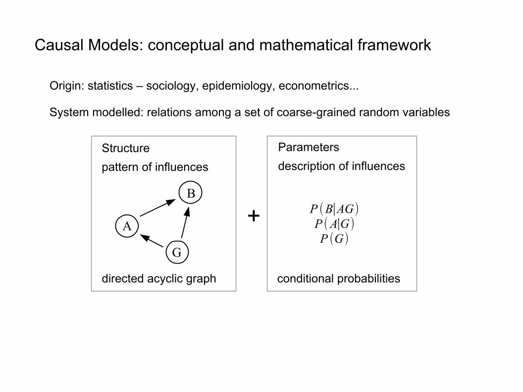
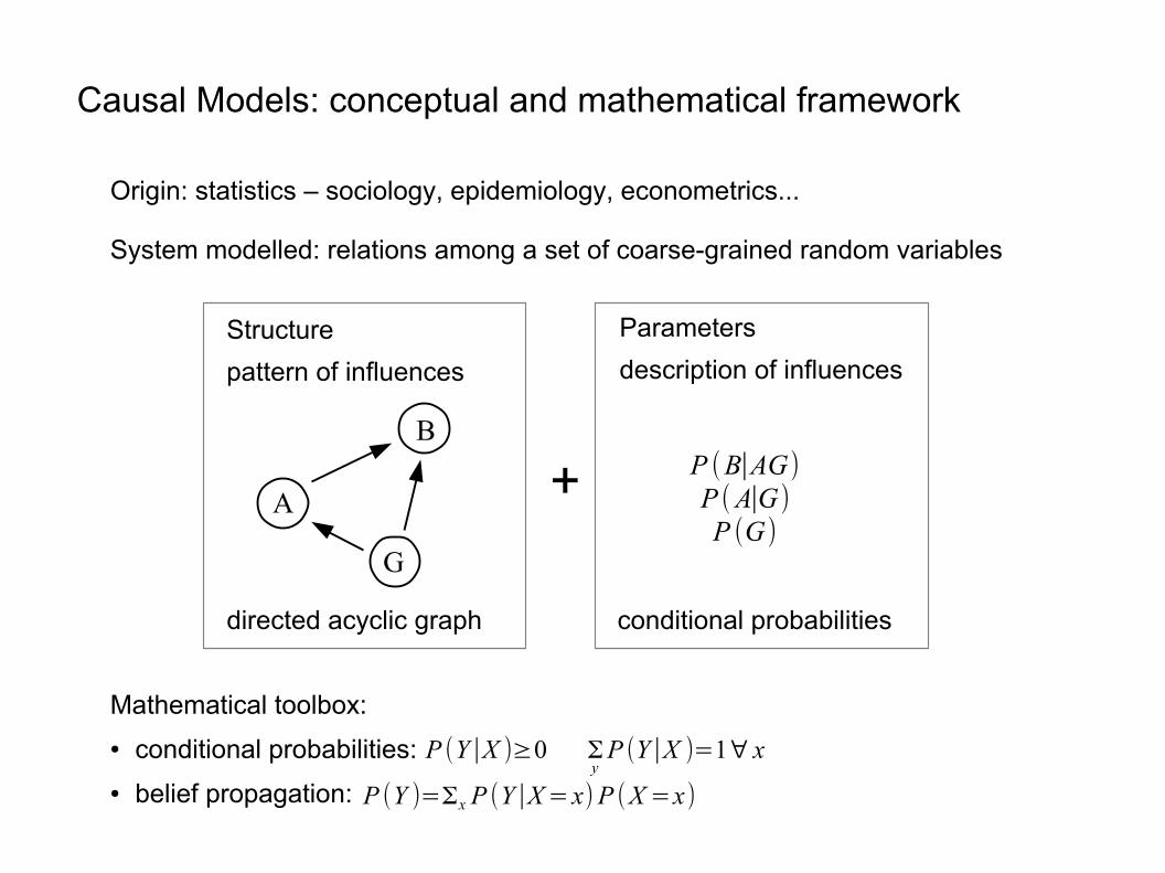
Causal Models: conceptual and mathematical framework
Origin: statistics – sociology, epidemiology, econometrics...
System modelled: relations among a set of coarse-grained random variables
Parameters
description of influences
Structure
pattern of influences
directed acyclic graph conditional probabilities
+ P (B∣AG)P (A∣G)P (G)
G
A
B
P (Y∣X )≥0 ΣyP (Y∣X )=1∀ x
Mathematical toolbox:
● conditional probabilities:
● belief propagation: P (Y )=Σx P (Y∣X=x)P (X=x)
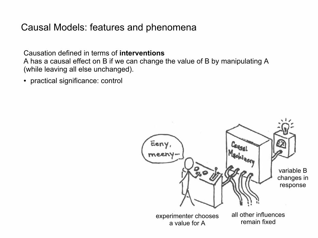
Causal Models: features and phenomena
experimenter choosesa value for A
all other influencesremain fixed
variable Bchanges inresponse
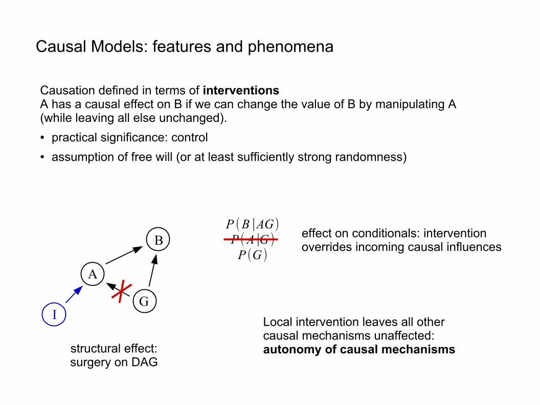
Causation defined in terms of interventionsA has a causal effect on B if we can change the value of B by manipulating A(while leaving all else unchanged).● practical significance: control
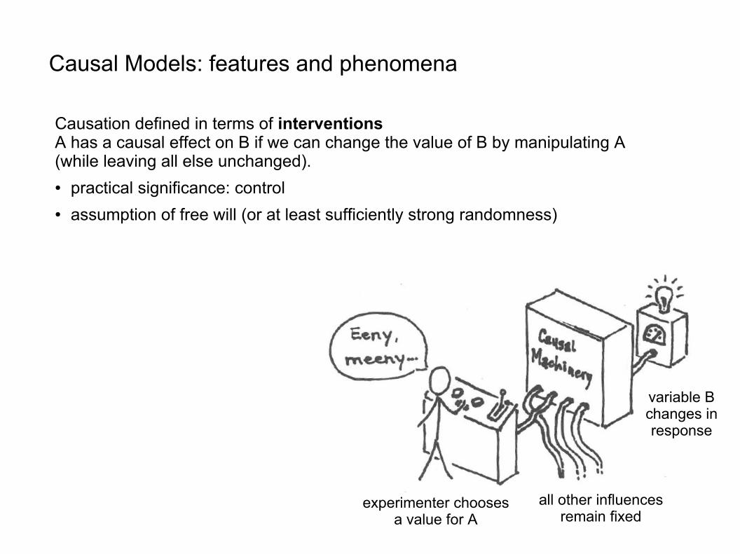
Causal Models: features and phenomena
experimenter choosesa value for A
all other influencesremain fixed
variable Bchanges inresponse
Causation defined in terms of interventionsA has a causal effect on B if we can change the value of B by manipulating A(while leaving all else unchanged).● practical significance: control● assumption of free will (or at least sufficiently strong randomness)
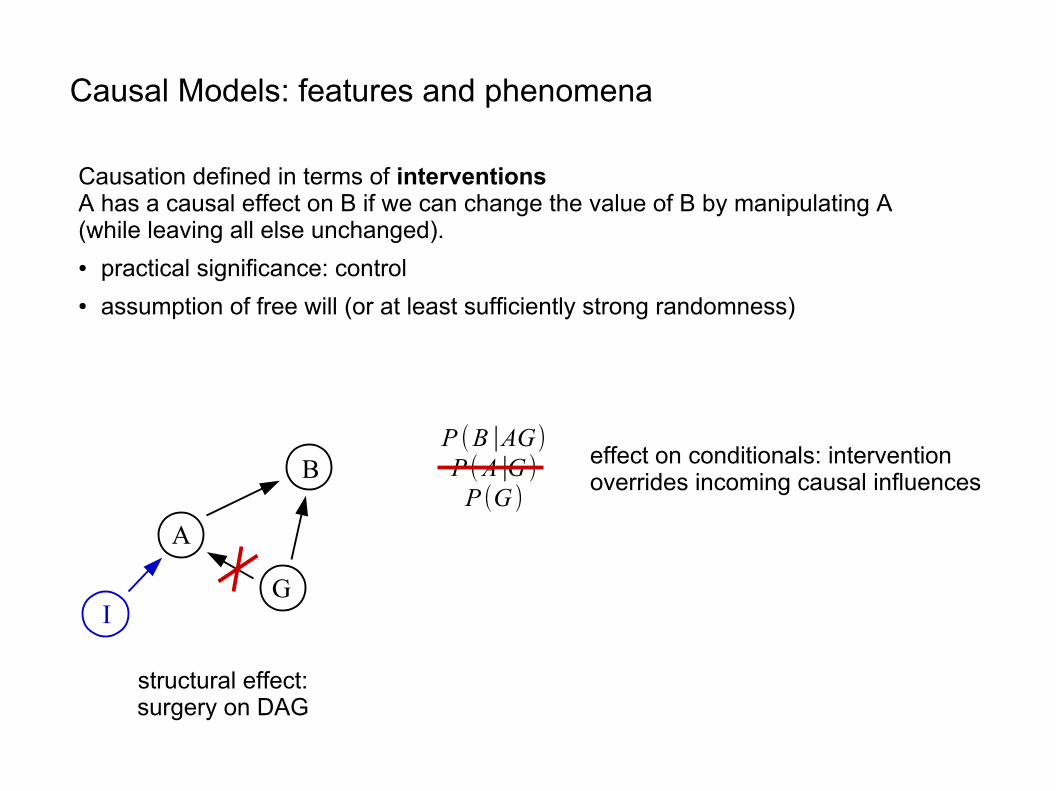
Causal Models: features and phenomena
Causation defined in terms of interventionsA has a causal effect on B if we can change the value of B by manipulating A(while leaving all else unchanged).● practical significance: control● assumption of free will (or at least sufficiently strong randomness)
G
A
B
I
structural effect:surgery on DAG
P (B∣AG)P (A∣G )P (G )
effect on conditionals: interventionoverrides incoming causal influences
Causal Models: features and phenomena
Causation defined in terms of interventionsA has a causal effect on B if we can change the value of B by manipulating A(while leaving all else unchanged).● practical significance: control● assumption of free will (or at least sufficiently strong randomness)
G
A
B
I
structural effect:surgery on DAG
P (B∣AG)P (A∣G )P (G )
Local intervention leaves all othercausal mechanisms unaffected: autonomy of causal mechanisms
effect on conditionals: interventionoverrides incoming causal influences
Causal Models: features and phenomena
G
A
B
I
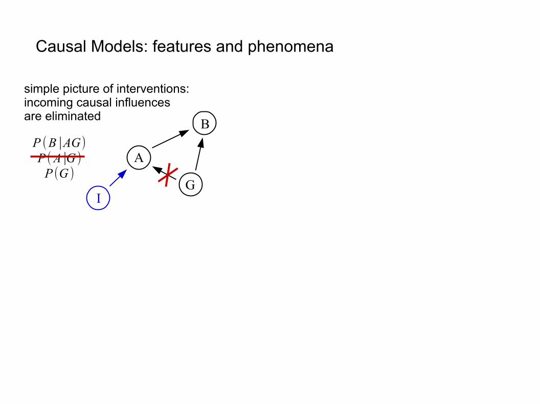
P (B∣AG)P (A∣G )P (G )
simple picture of interventions:incoming causal influencesare eliminated
Causal Models: features and phenomena
G
A1
B
A2
I
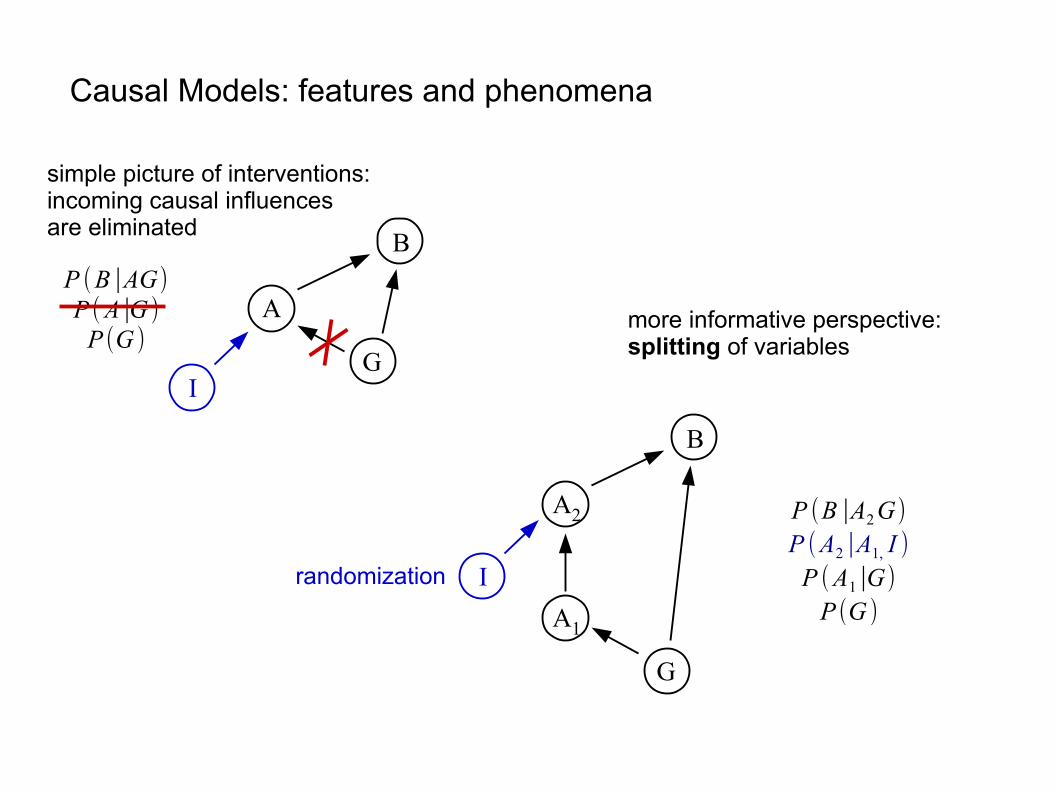
P (B ∣A2G)P (A2∣A1, I )P (A1∣G)P (G )
G
A
B
I
P (B∣AG)P (A∣G )P (G )
simple picture of interventions:incoming causal influencesare eliminated
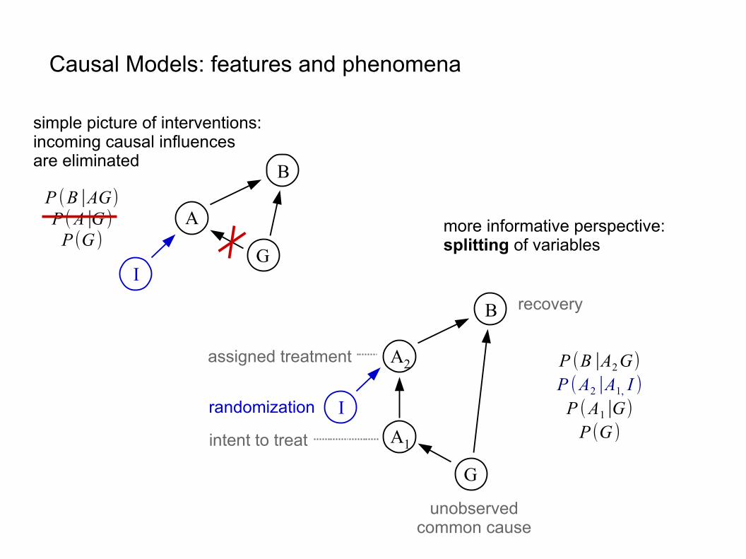
more informative perspective:splitting of variables
randomization
Causal Models: features and phenomena
G
A1
B
A2
I
P (B ∣A2G)P (A2∣A1, I )P (A1∣G)P (G )
G
A
B
I
P (B∣AG)P (A∣G )P (G )
simple picture of interventions:incoming causal influencesare eliminated
more informative perspective:splitting of variables
assigned treatment
intent to treat
randomization
recovery
unobservedcommon cause
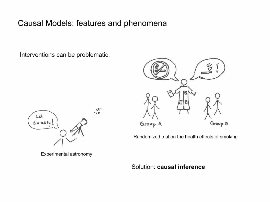
Causal Models: features and phenomena
Interventions can be problematic.
Randomized trial on the health effects of smoking
Experimental astronomy
Solution: causal inference
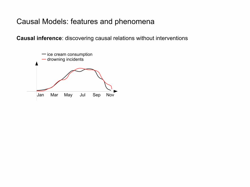
Jan Mar May Jul Sep Nov
ice cream consumptiondrowning incidents
Causal Models: features and phenomena
Causal inference: discovering causal relations without interventions
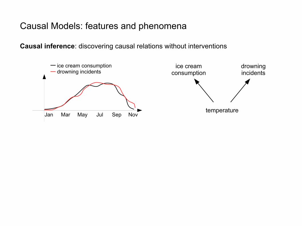
ice creamconsumption
drowningincidents
temperatureJan Mar May Jul Sep Nov
ice cream consumptiondrowning incidents
Causal Models: features and phenomena
Causal inference: discovering causal relations without interventions
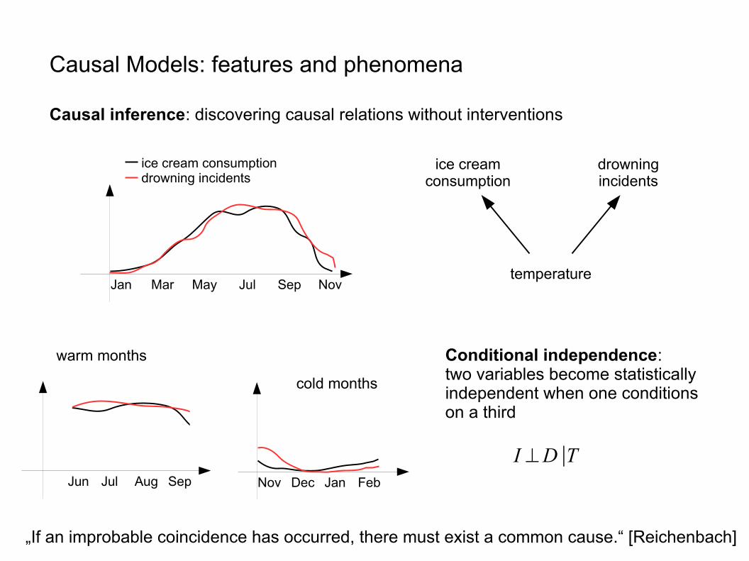
Jun Jul Aug Sep
warm months
ice creamconsumption
drowningincidents
temperature
Nov Dec Jan Feb
cold months
Conditional independence: two variables become statisticallyindependent when one conditionson a third
Jan Mar May Jul Sep Nov
ice cream consumptiondrowning incidents
Causal Models: features and phenomena
Causal inference: discovering causal relations without interventions
„If an improbable coincidence has occurred, there must exist a common cause.“ [Reichenbach]
I ⊥D∣T
Causal Models: features and phenomena
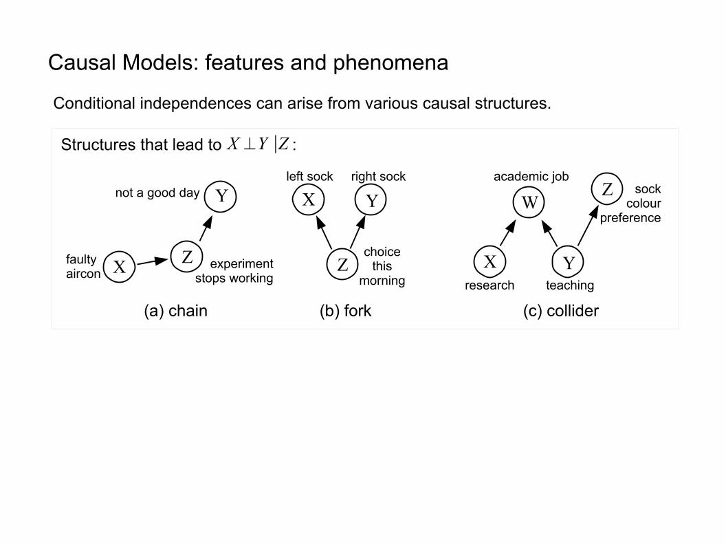
Conditional independences can arise from various causal structures.
W
X Y
Zacademic job
research teaching
sockcolour
preference
X ⊥Y ∣Z
(a) chain (b) fork (c) collider
Z
X Y
left sock right sock
choicethis
morning
ZX
Ynot a good day
experimentstops working
faultyaircon
Structures that lead to :
Causal Models: features and phenomena
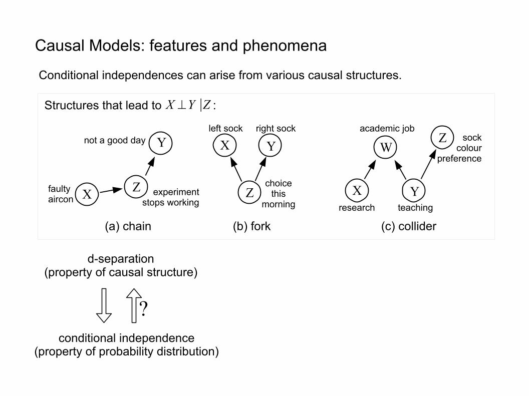
Conditional independences can arise from various causal structures.
W
X Y
Zacademic job
research teaching
sockcolour
preference
faithfulness/stability [Def 2.4.1]:a model generates a stabledistribution if the set ofconditional independencesremains unchanged underchanges of parametrization(conditionals)Example of unstable conditionalindependences: twoequiprobably coins and C=A+B(mod2)
d-separation(property of causal structure)
conditional independence(property of probability distribution)
?
X ⊥Y ∣Z
(a) chain (b) fork (c) collider
Z
X Y
left sock right sock
choicethis
morning
ZX
Ynot a good day
experimentstops working
faultyaircon
Structures that lead to :
Causal Models: features and phenomena
Conditional independences can arise from various causal structures.
W
X Y
Zacademic job
research teaching
sockcolour
preference
d-separation(property of causal structure)
conditional independence(property of probability distribution)
?
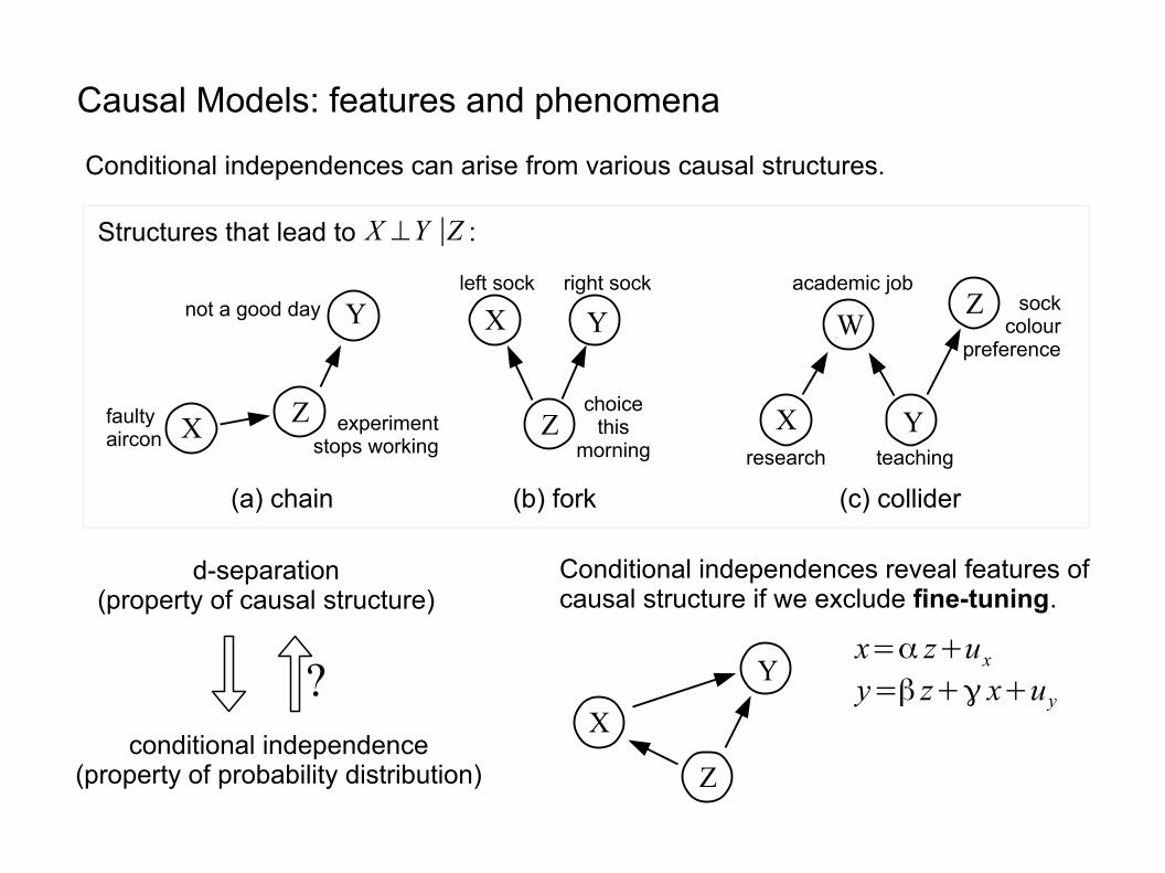
Conditional independences reveal features ofcausal structure if we exclude fine-tuning.
X ⊥Y ∣Z
(a) chain (b) fork (c) collider
x=α z+ux
y=β z+γ x+uy
Z
X
Y
Z
X Y
left sock right sock
choicethis
morning
ZX
Ynot a good day
experimentstops working
faultyaircon
Structures that lead to :
Causal Models: features and phenomena
Conditional independences can arise from various causal structures.
W
X Y
Zacademic job
research teaching
sockcolour
preference
faithfulness/stability [Def 2.4.1]:a model generates a stabledistribution if the set ofconditional independencesremains unchanged underchanges of parametrization(conditionals)Example of unstable conditionalindependences: twoequiprobably coins and C=A+B(mod2)
d-separation(property of causal structure)
conditional independence(property of probability distribution)
?
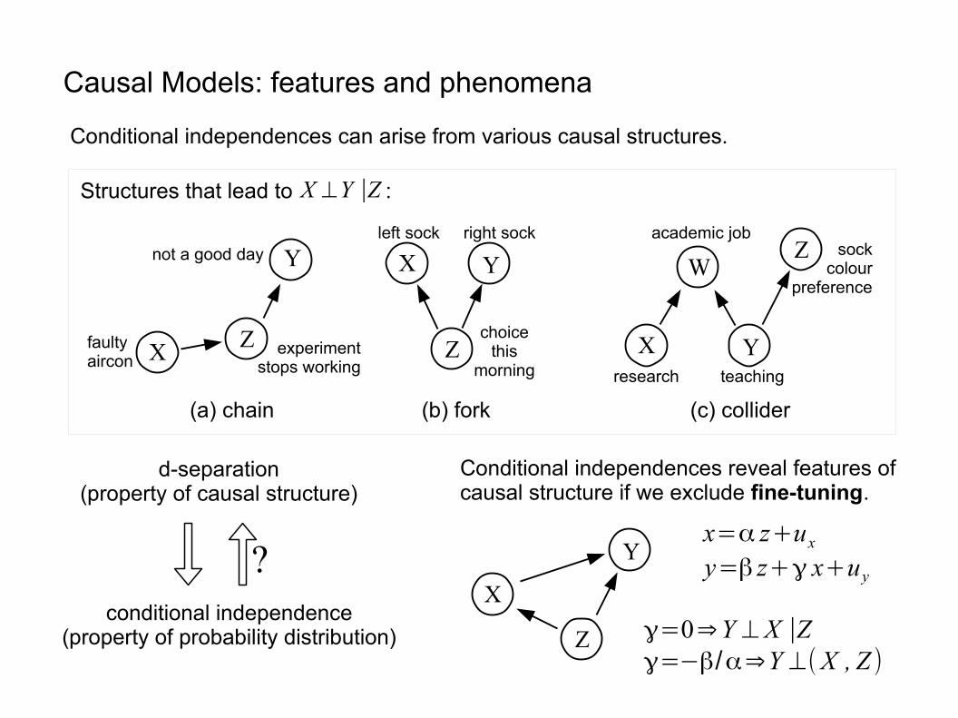
Conditional independences reveal features ofcausal structure if we exclude fine-tuning.
X ⊥Y ∣Z
(a) chain (b) fork (c) collider
x=α z+ux
y=β z+γ x+uy
Z
X
Y
Z
X Y
left sock right sock
choicethis
morning
ZX
Ynot a good day
experimentstops working
faultyaircon
Structures that lead to :
γ=0⇒Y ⊥ X ∣Zγ=−β/α⇒Y ⊥(X , Z )
Causal Models: features and phenomena
uG
G
A
B
uA
uB
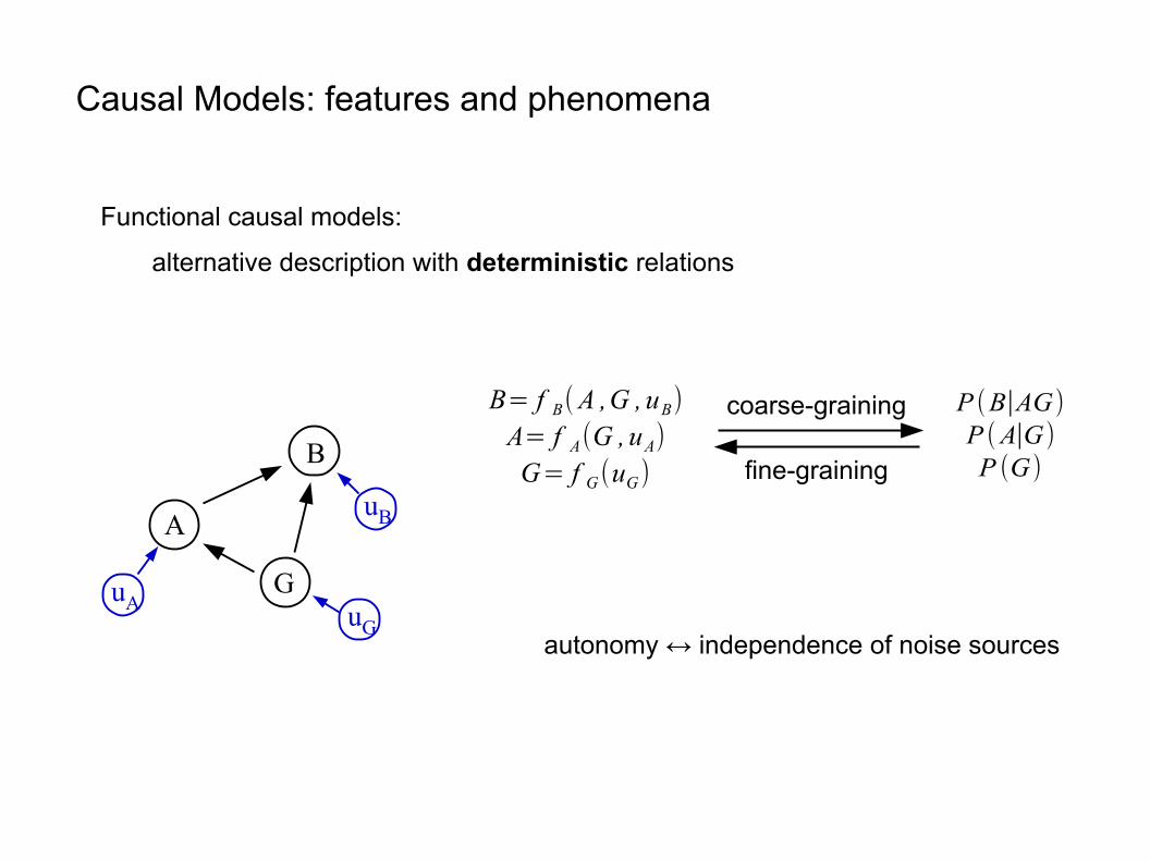
P (B∣AG)P (A∣G)P (G)
B= f B(A ,G ,uB)A= f A(G ,uA)G= f G(uG)
Functional causal models:
alternative description with deterministic relations
coarse-graining
fine-graining
autonomy ↔ independence of noise sources
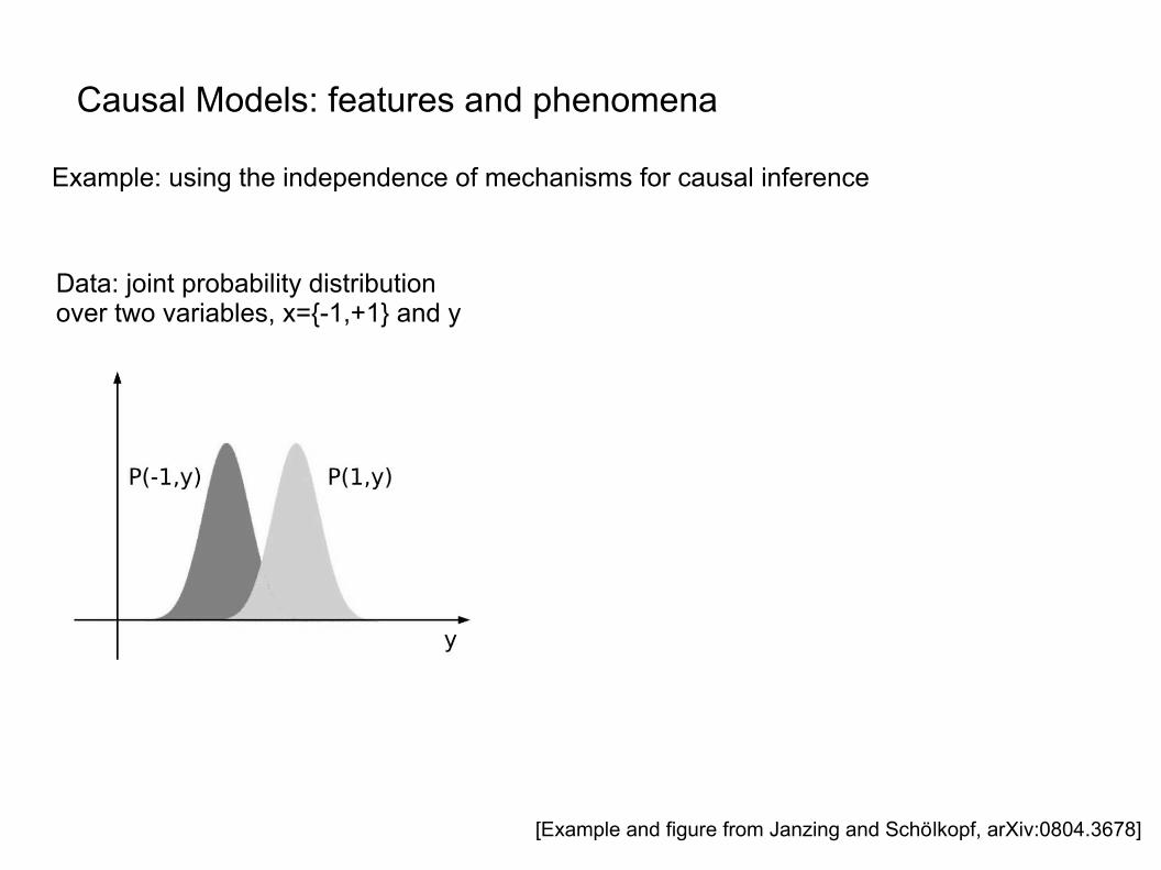
Causal Models: features and phenomena
Data: joint probability distributionover two variables, x={-1,+1} and y
[Example and figure from Janzing and Schölkopf, arXiv:0804.3678]
Example: using the independence of mechanisms for causal inference
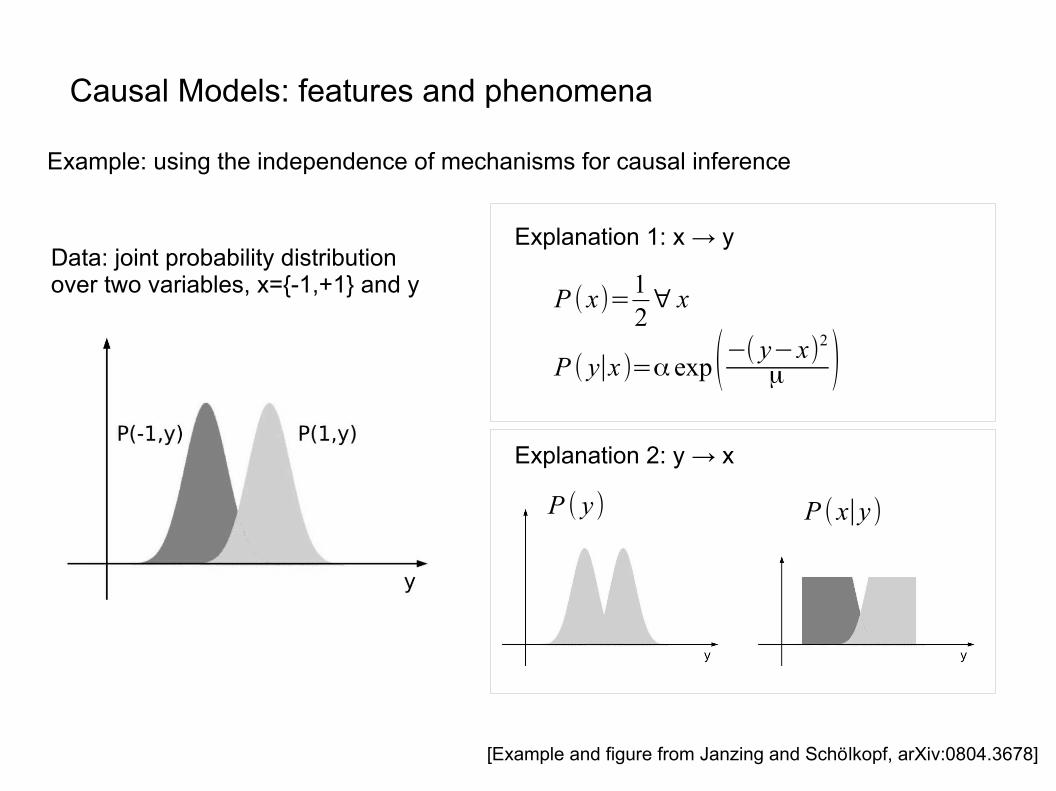
Causal Models: features and phenomena
Data: joint probability distributionover two variables, x={-1,+1} and y
[Example and figure from Janzing and Schölkopf, arXiv:0804.3678]
Explanation 1: x → y
P ( x)=12∀ x
P ( y∣x )=α exp(−( y−x)2μ )
Explanation 2: y → x
P ( y ) P (x∣y )
Example: using the independence of mechanisms for causal inference
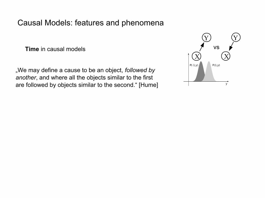
Causal Models: features and phenomena
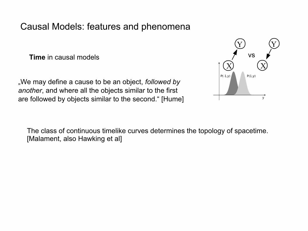
Time in causal models
„We may define a cause to be an object, followed byanother, and where all the objects similar to the firstare followed by objects similar to the second.“ [Hume]
X
Y
X
Yvs
Causal Models: features and phenomena
Time in causal models
„We may define a cause to be an object, followed byanother, and where all the objects similar to the firstare followed by objects similar to the second.“ [Hume]
X
Y
X
Yvs
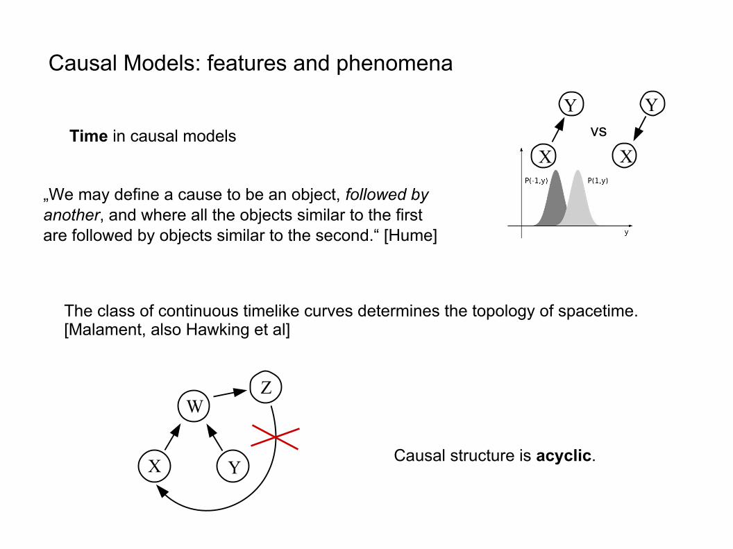
The class of continuous timelike curves determines the topology of spacetime.[Malament, also Hawking et al]
Causal Models: features and phenomena
Time in causal models
„We may define a cause to be an object, followed byanother, and where all the objects similar to the firstare followed by objects similar to the second.“ [Hume]
X
Y
X
Yvs
The class of continuous timelike curves determines the topology of spacetime.[Malament, also Hawking et al]
Causal structure is acyclic.
W
X Y
Z
Causal Models: features and phenomena
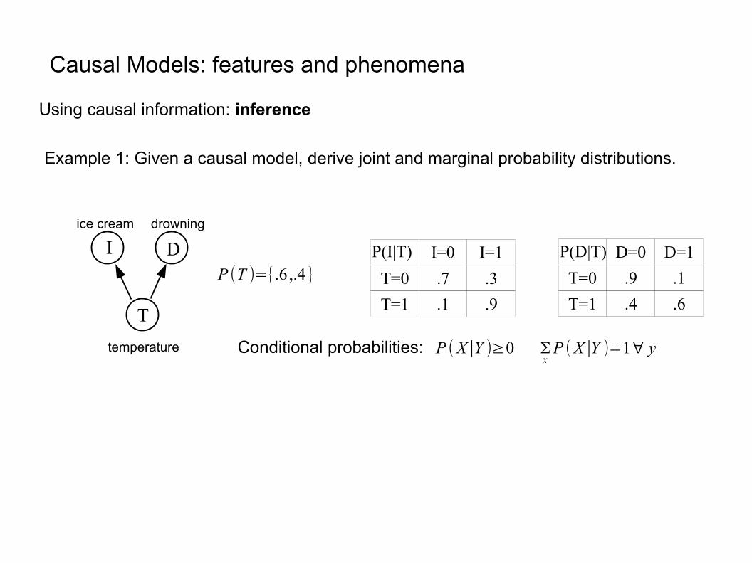
Using causal information: inference
Example 1: Given a causal model, derive joint and marginal probability distributions.
T
I D
ice cream drowning
temperature
P (T )={.6 ,.4 }I=0 I=1
T=0 .7 .3
T=1 .1 .9
P(I|T) D=0 D=1
T=0 .9 .1
T=1 .4 .6
P(D|T)
P (X∣Y )≥0 ΣxP (X∣Y )=1∀ yConditional probabilities:
Causal Models: features and phenomena
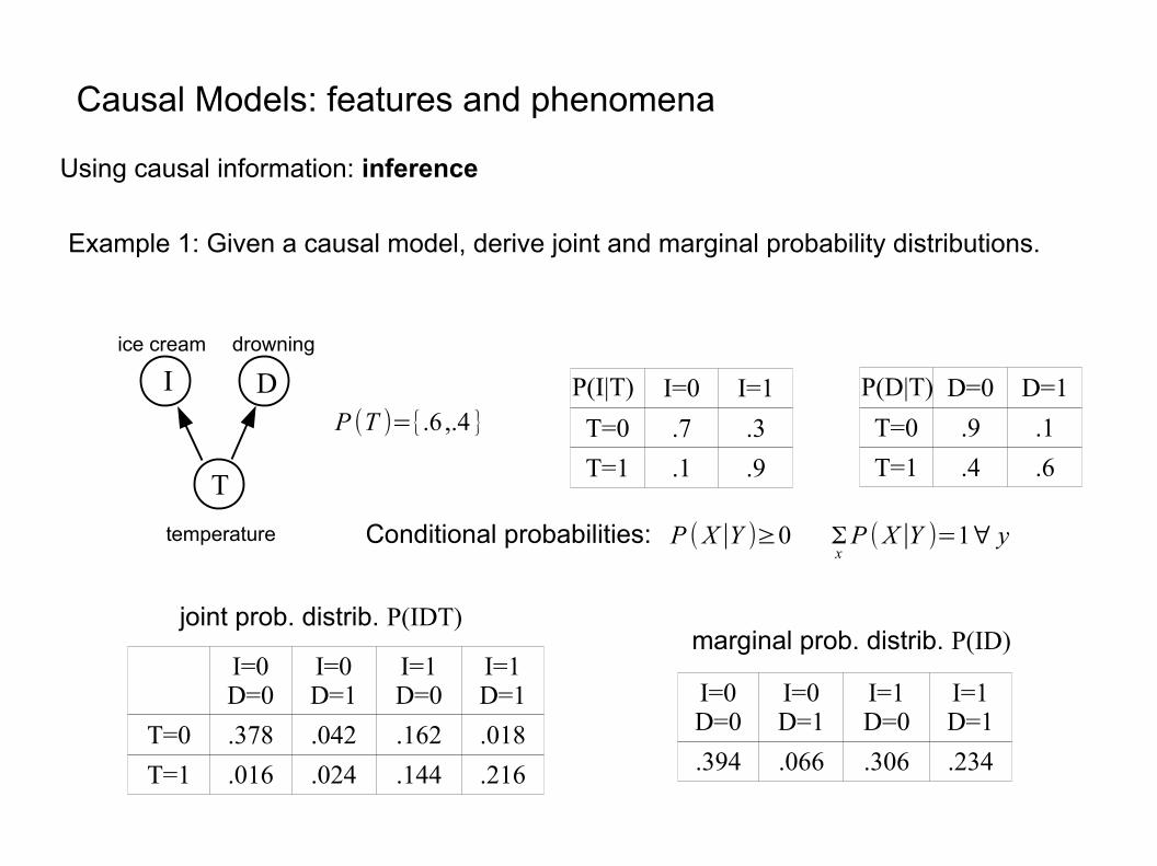
Using causal information: inference
Example 1: Given a causal model, derive joint and marginal probability distributions.
T
I D
ice cream drowning
temperature
P (T )={.6 ,.4 }I=0 I=1
T=0 .7 .3
T=1 .1 .9
P(I|T) D=0 D=1
T=0 .9 .1
T=1 .4 .6
P(D|T)
I=0D=0
I=0D=1
I=1D=0
I=1D=1
T=0 .378 .042 .162 .018
T=1 .016 .024 .144 .216
I=0D=0
I=0D=1
I=1D=0
I=1D=1
.394 .066 .306 .234
marginal prob. distrib. P(ID)joint prob. distrib. P(IDT)
P (X∣Y )≥0 ΣxP (X∣Y )=1∀ yConditional probabilities:
Causal Models: features and phenomena
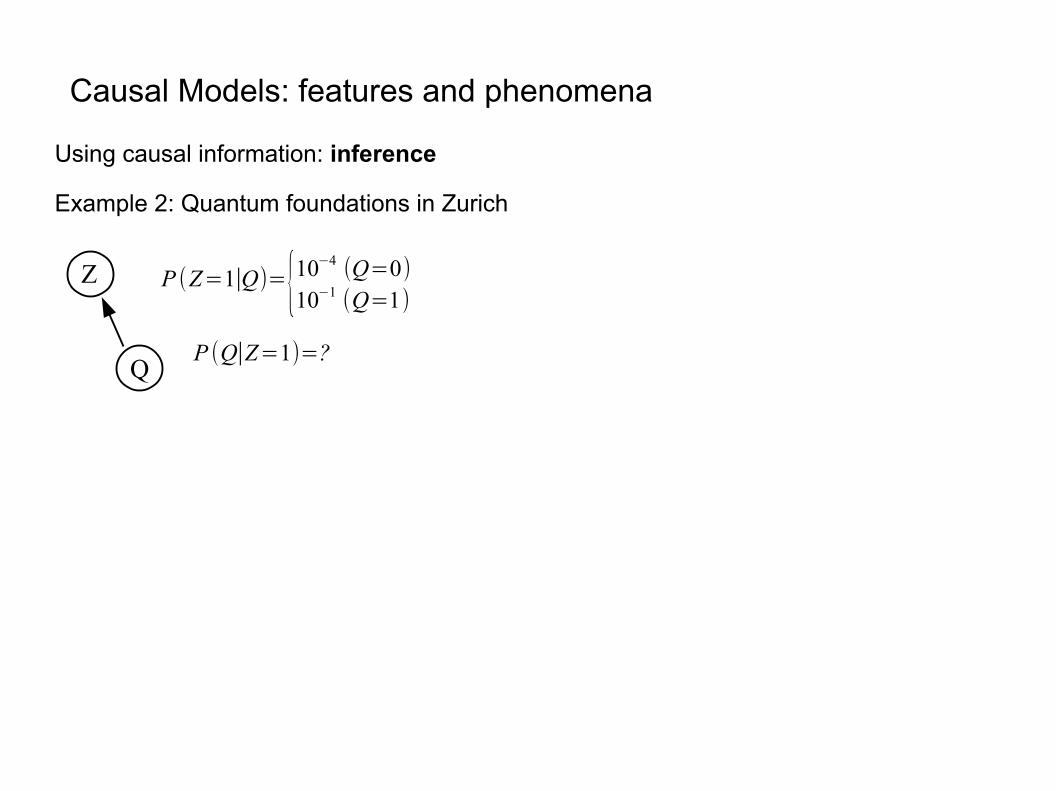
Using causal information: inference
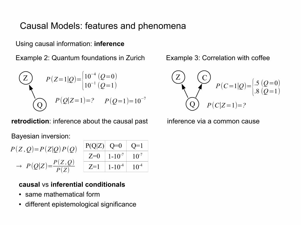
Example 2: Quantum foundations in Zurich
P (Z=1∣Q)={10−4 (Q=0)10−1 (Q=1)
P (Q∣Z=1)=?Q
Z
Causal Models: features and phenomena
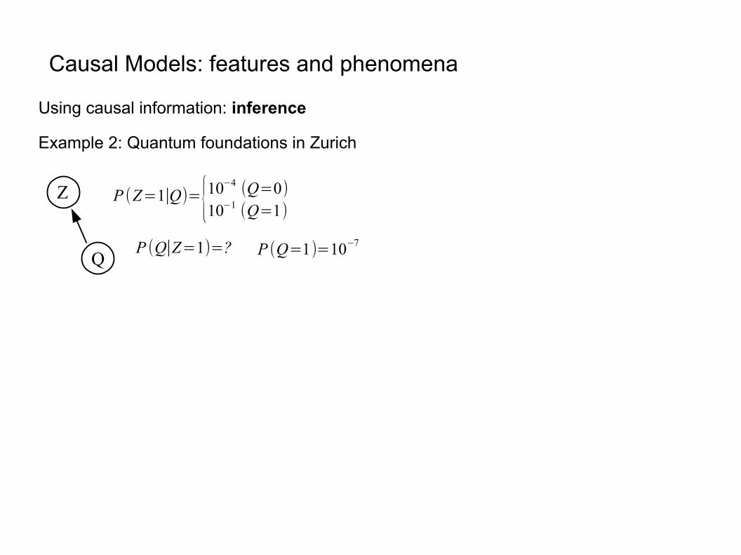
Using causal information: inference
Example 2: Quantum foundations in Zurich
P (Q=1)=10−7
P (Z=1∣Q)={10−4 (Q=0)10−1 (Q=1)
P (Q∣Z=1)=?Q
Z
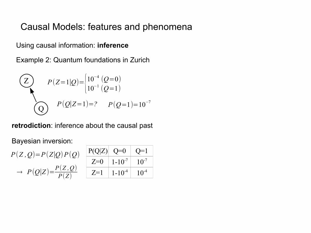
Causal Models: features and phenomena
Using causal information: inference
Example 2: Quantum foundations in Zurich
P (Q=1)=10−7
P (Z=1∣Q)={10−4 (Q=0)10−1 (Q=1)
P (Z ,Q)=P (Z∣Q)P (Q)
P (Q∣Z=1)=?
retrodiction: inference about the causal past
→ P (Q∣Z )=P (Z ,Q)P (Z )
Bayesian inversion:Q=0 Q=1
Z=0 1-10-7 10-7
Z=1 1-10-4 10-4
P(Q|Z)
Q
Z
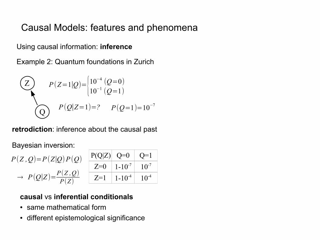
Causal Models: features and phenomena
Using causal information: inference
Example 2: Quantum foundations in Zurich
P (Q=1)=10−7
P (Z=1∣Q)={10−4 (Q=0)10−1 (Q=1)
P (Z ,Q)=P (Z∣Q)P (Q)
P (Q∣Z=1)=?
retrodiction: inference about the causal past
causal vs inferential conditionals● same mathematical form● different epistemological significance
→ P (Q∣Z )=P (Z ,Q)P (Z )
Bayesian inversion:Q=0 Q=1
Z=0 1-10-7 10-7
Z=1 1-10-4 10-4
P(Q|Z)
Q
Z
Q
Z CP (C=1∣Q)={.5 (Q=0)
.8 (Q=1)
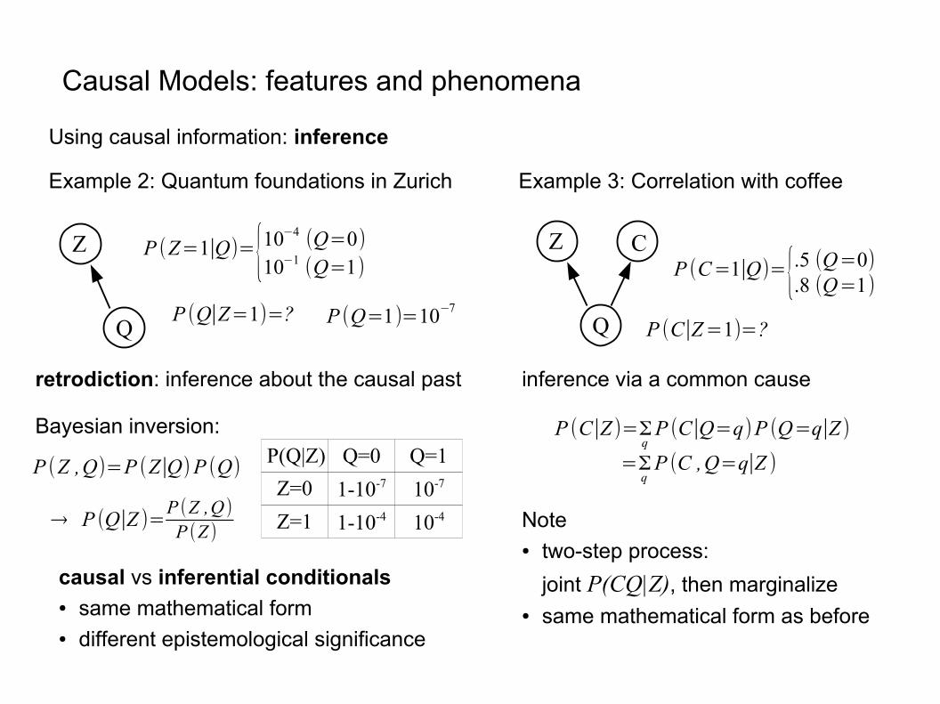
Example 3: Correlation with coffee
P (C∣Z=1)=?
inference via a common cause
Causal Models: features and phenomena
Using causal information: inference
Example 2: Quantum foundations in Zurich
P (Q=1)=10−7
P (Z=1∣Q)={10−4 (Q=0)10−1 (Q=1)
P (Z ,Q)=P (Z∣Q)P (Q)
P (Q∣Z=1)=?
retrodiction: inference about the causal past
causal vs inferential conditionals● same mathematical form● different epistemological significance
→ P (Q∣Z )=P (Z ,Q)P (Z )
Bayesian inversion:Q=0 Q=1
Z=0 1-10-7 10-7
Z=1 1-10-4 10-4
P(Q|Z)
Q
Z
Q
Z CP (C=1∣Q)={.5 (Q=0)
.8 (Q=1)
Example 3: Correlation with coffee
P (C∣Z=1)=?
P (C∣Z )=ΣqP (C∣Q=q)P (Q=q∣Z )
=ΣqP (C ,Q=q∣Z )
inference via a common cause
Note● two-step process:
joint P(CQ|Z), then marginalize● same mathematical form as before
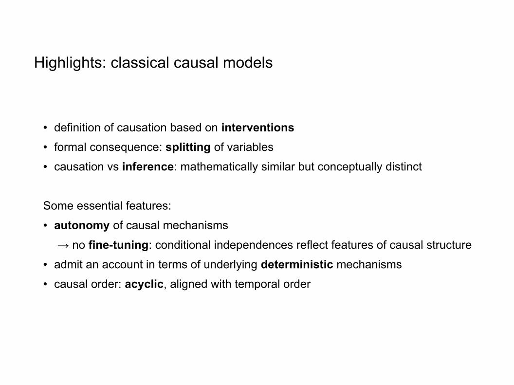
Highlights: classical causal models
● definition of causation based on interventions
● formal consequence: splitting of variables
● causation vs inference: mathematically similar but conceptually distinct
Some essential features:
● autonomy of causal mechanisms
→ no fine-tuning: conditional independences reflect features of causal structure
● admit an account in terms of underlying deterministic mechanisms
● causal order: acyclic, aligned with temporal order
Quantum Indeterminism
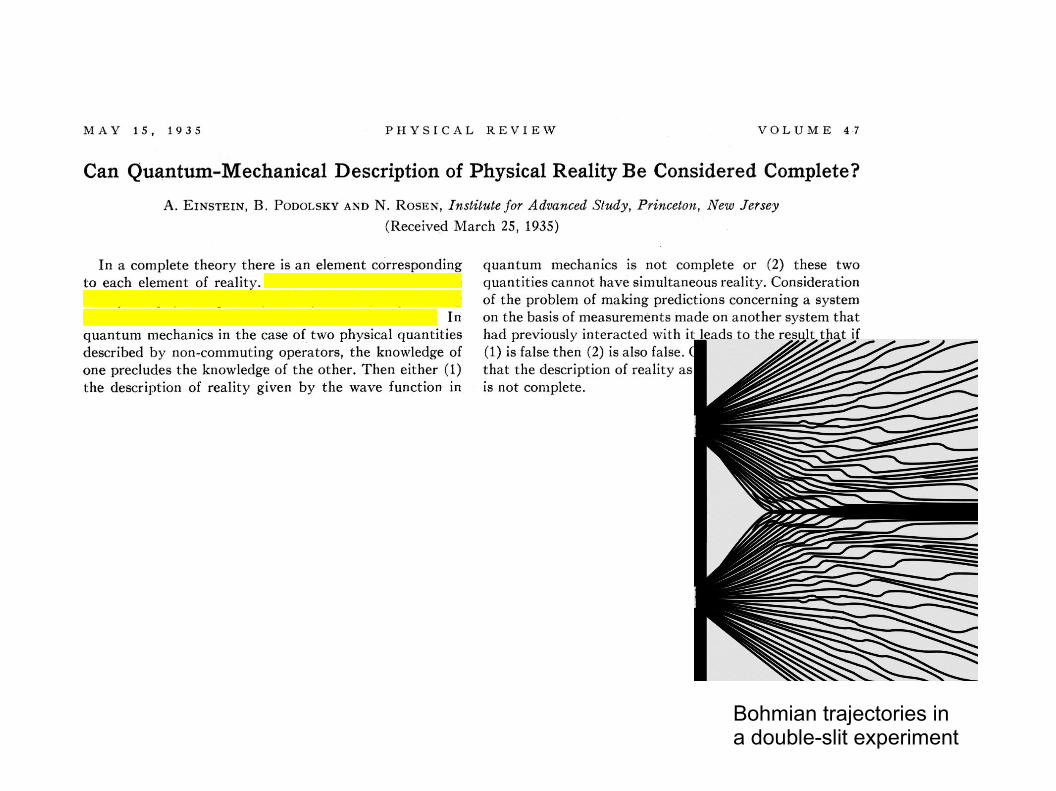
Bohmian trajectories ina double-slit experiment
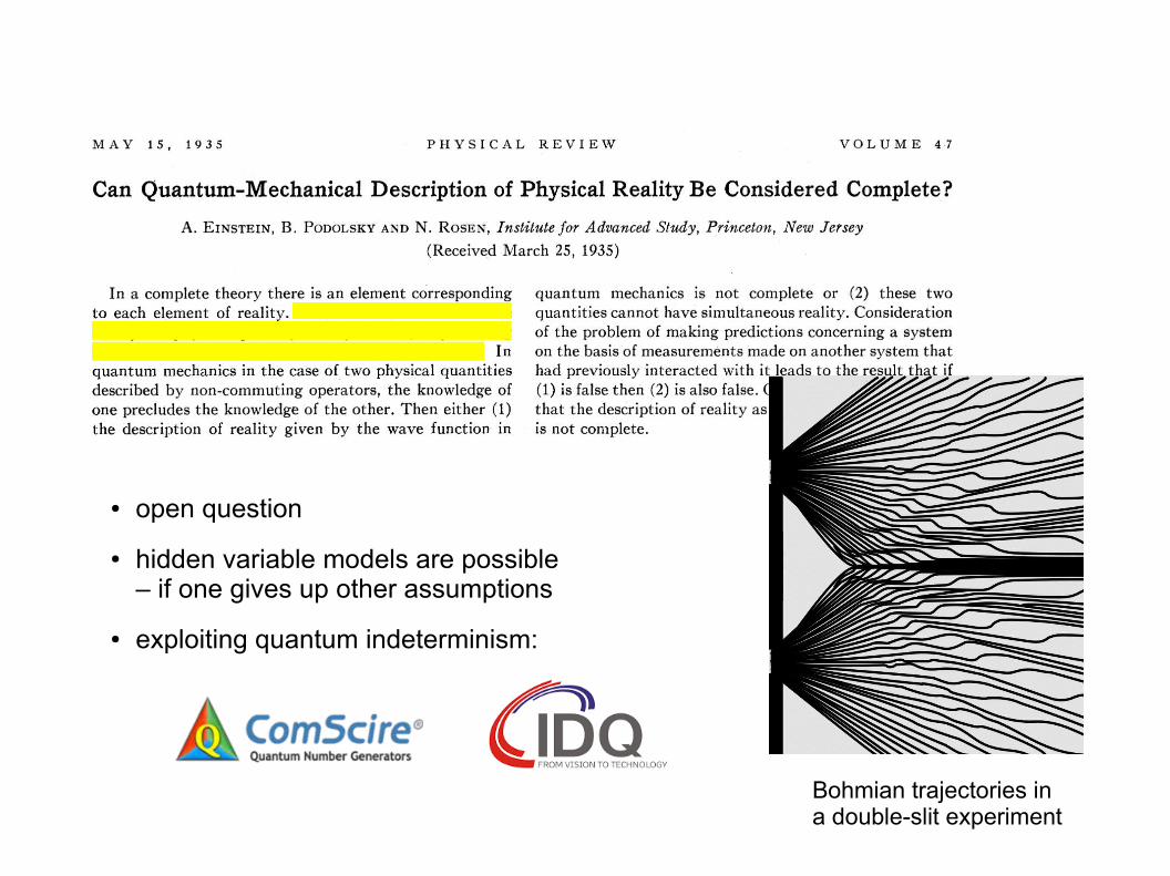
Bohmian trajectories ina double-slit experiment
● open question
● hidden variable models are possible– if one gives up other assumptions
● exploiting quantum indeterminism:
Retrocausalityand Causal Loops
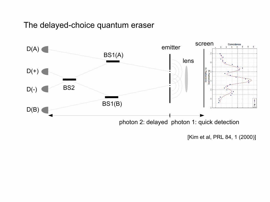
The delayed-choice quantum eraser
BS1(A)
BS1(B)
BS2
D(A)
D(+)
D(-)
D(B)
lens
[Kim et al, PRL 84, 1 (2000)]
emitterscreen
photon 1: quick detectionphoton 2: delayed
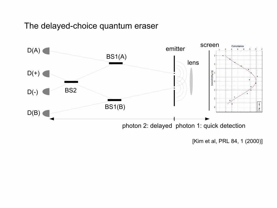
The delayed-choice quantum eraser
BS1(A)
BS1(B)
BS2
D(A)
D(+)
D(-)
D(B)
lens
[Kim et al, PRL 84, 1 (2000)]
emitterscreen
photon 1: quick detectionphoton 2: delayed
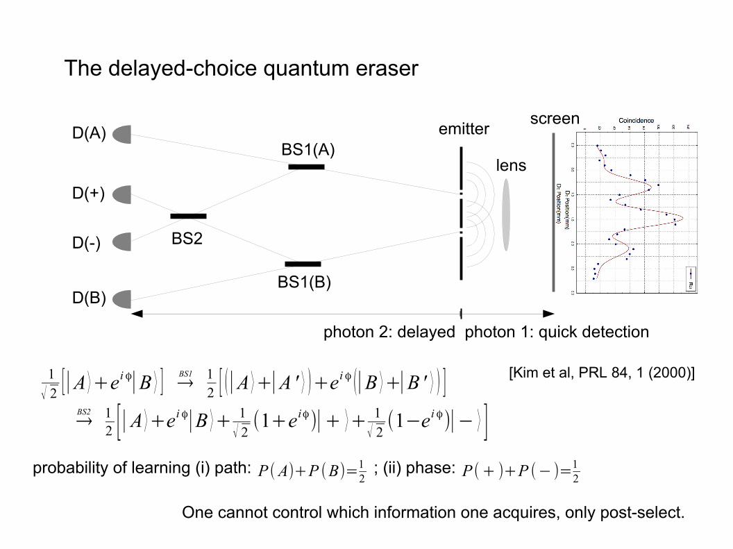
The delayed-choice quantum eraser
BS1(A)
BS1(B)
BS2
D(A)
D(+)
D(-)
D(B)
lens
[Kim et al, PRL 84, 1 (2000)]1
√ 2[∣A ⟩+ei ϕ∣B ⟩ ] →BS1 1
2 [ (∣A ⟩+∣A' ⟩ )+ei ϕ (∣B ⟩+∣B' ⟩ ) ]→BS2 1
2 [∣A ⟩+ei ϕ∣B ⟩+ 1
√ 2(1+eiϕ)∣+ ⟩+ 1
√ 2(1−ei ϕ)∣− ⟩ ]
emitterscreen
photon 1: quick detectionphoton 2: delayed
One cannot control which information one acquires, only post-select.
probability of learning (i) path: ; (ii) phase: P(A)+P (B)=12 P(+ )+P (−)=1
2
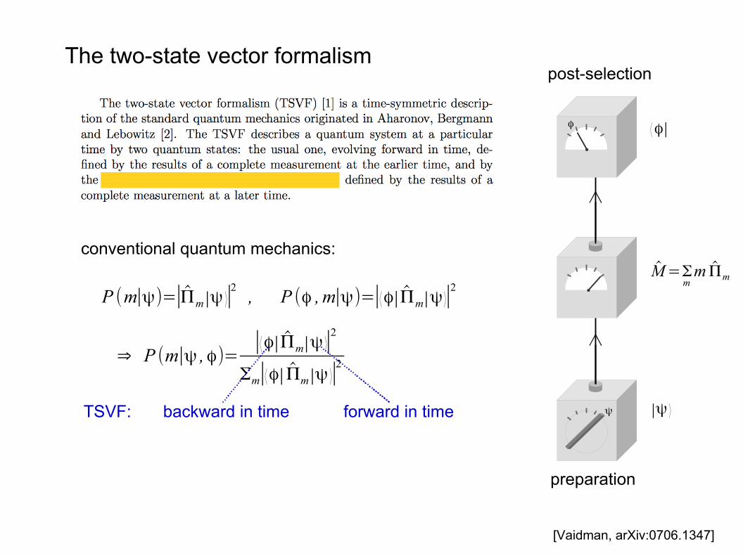
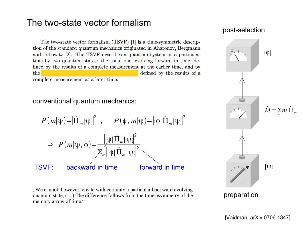
The two-state vector formalism
ψ
ϕ
M=Σmm Πm
preparation
post-selection
∣ψ ⟩
⟨ϕ∣
conventional quantum mechanics:
P (m∣ψ)=∣Πm∣ψ ⟩∣2 , P (ϕ , m∣ψ)=∣⟨ϕ∣Πm∣ψ ⟩∣2
⇒ P (m∣ψ ,ϕ)=∣⟨ϕ∣Πm∣ψ ⟩∣2
Σm∣⟨ϕ∣Πm∣ψ ⟩∣2
forward in timebackward in timeTSVF:
[Vaidman, arXiv:0706.1347]
The two-state vector formalism
ψ
ϕ
M=Σmm Πm
preparation
post-selection
∣ψ ⟩
⟨ϕ∣
conventional quantum mechanics:
P (m∣ψ)=∣Πm∣ψ ⟩∣2 , P (ϕ , m∣ψ)=∣⟨ϕ∣Πm∣ψ ⟩∣2
⇒ P (m∣ψ ,ϕ)=∣⟨ϕ∣Πm∣ψ ⟩∣2
Σm∣⟨ϕ∣Πm∣ψ ⟩∣2
forward in timebackward in timeTSVF:
„We cannot, however, create with certainty a particular backward evolvingquantum state, (…) The difference follows from the time asymmetry of thememory arrow of time.“
[Vaidman, arXiv:0706.1347]
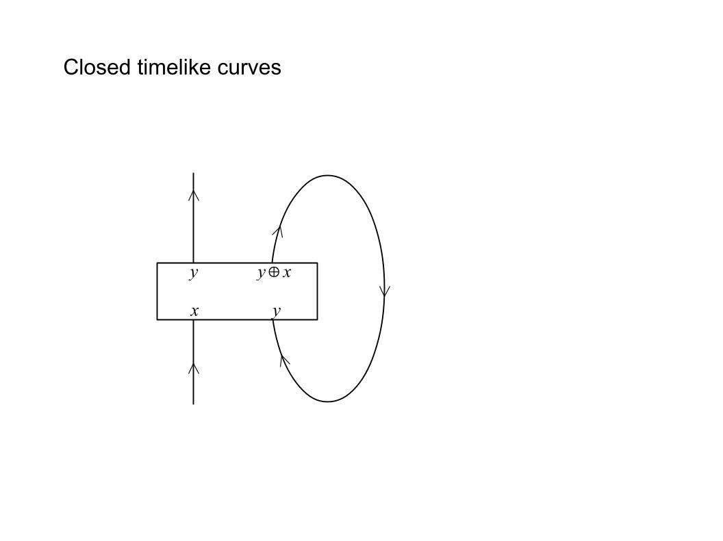
Closed timelike curves
y⊕x
yx
y
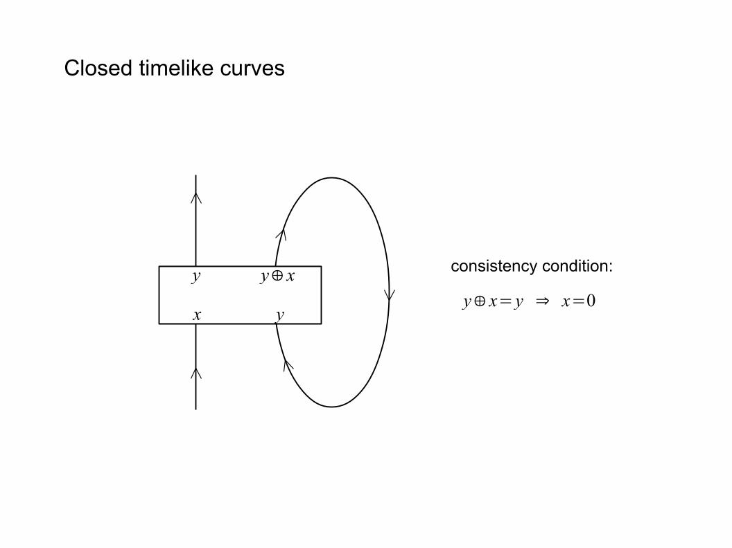
Closed timelike curves
y⊕x=y ⇒ x=0
consistency condition:y⊕x
yx
y
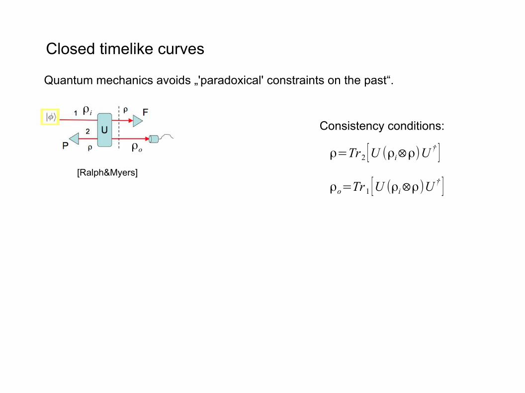
Closed timelike curves
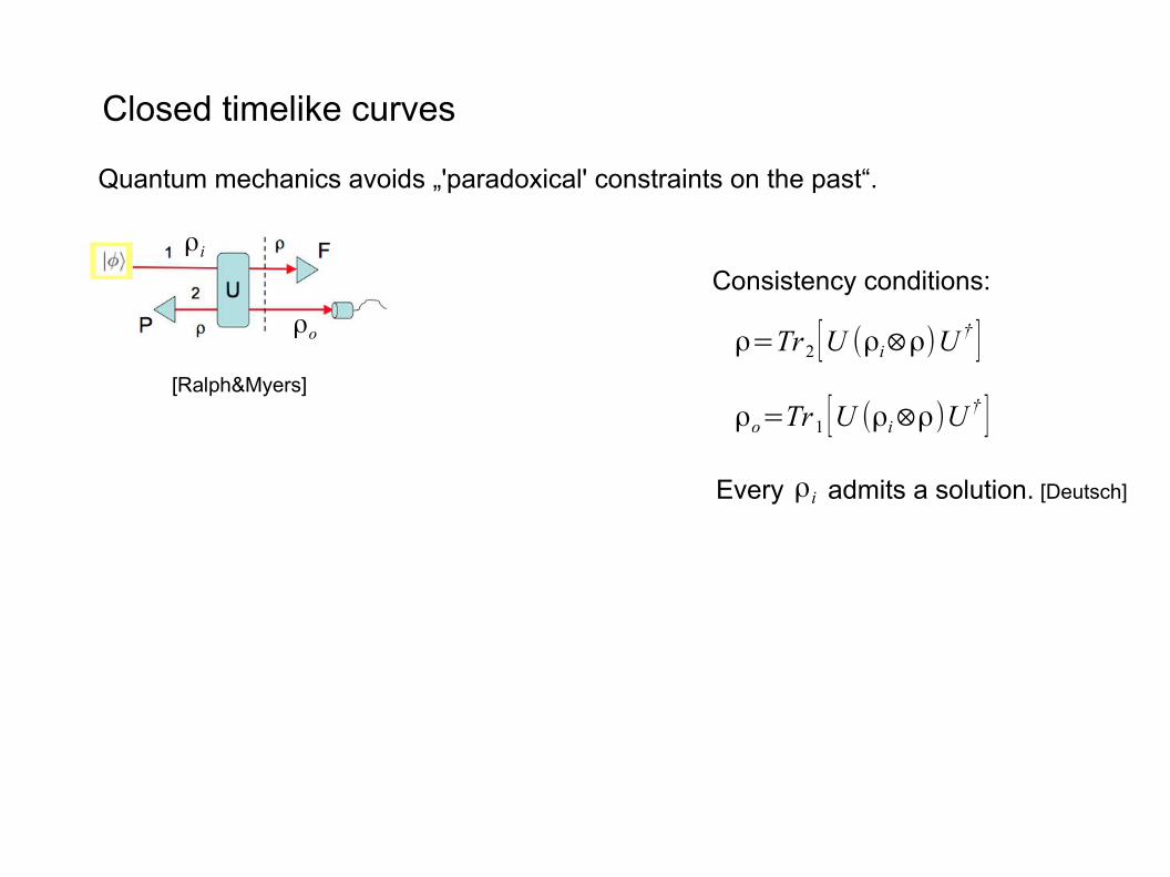
Consistency conditions:
ρ=Tr2 [U (ρi⊗ρ)U† ]
ρo=Tr1 [U (ρi⊗ρ)U† ]
ρo
ρi
Quantum mechanics avoids „'paradoxical' constraints on the past“.
[Ralph&Myers]
Closed timelike curves
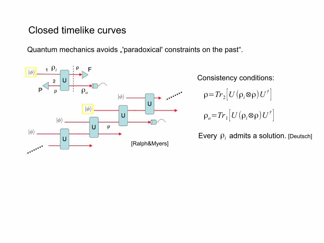
Consistency conditions:
ρ=Tr2 [U (ρi⊗ρ)U† ]
ρo=Tr1 [U (ρi⊗ρ)U† ]
ρo
ρi
Every admits a solution. [Deutsch]ρi
Quantum mechanics avoids „'paradoxical' constraints on the past“.
[Ralph&Myers]
Closed timelike curves
Consistency conditions:
ρ=Tr2 [U (ρi⊗ρ)U† ]
ρo=Tr1 [U (ρi⊗ρ)U† ]
ρo
ρi
[Ralph&Myers]Every admits a solution. [Deutsch]ρi
Quantum mechanics avoids „'paradoxical' constraints on the past“.
Closed timelike curves
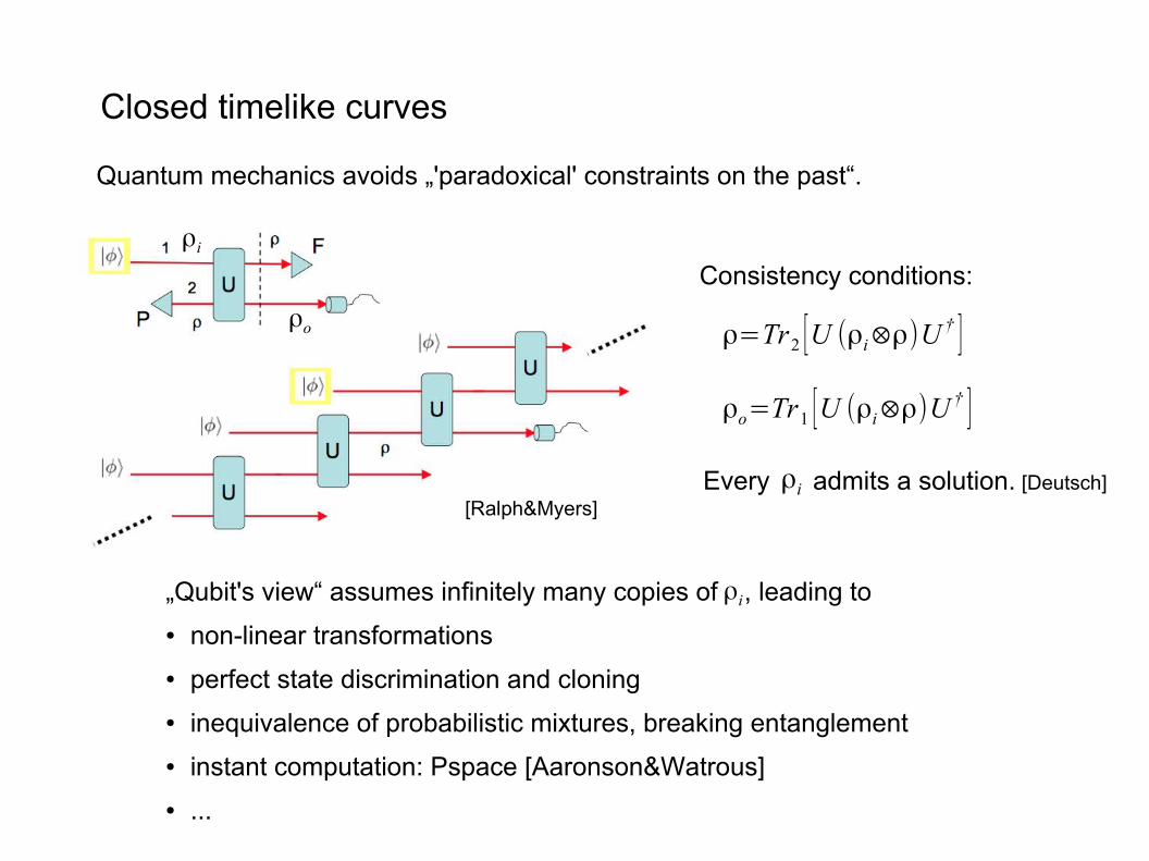
Consistency conditions:
ρ=Tr2 [U (ρi⊗ρ)U† ]
ρo=Tr1 [U (ρi⊗ρ)U† ]
ρo
ρi
[Ralph&Myers]Every admits a solution. [Deutsch]ρi
Quantum mechanics avoids „'paradoxical' constraints on the past“.
ρi„Qubit's view“ assumes infinitely many copies of , leading to
● non-linear transformations
● perfect state discrimination and cloning
● inequivalence of probabilistic mixtures, breaking entanglement
● instant computation: Pspace [Aaronson&Watrous]
● ...
problems solved andpersisting:- grandfather paradox: solvedby demanding consistency- retrocausal constraints onpast: solved by showing thatall inputs admit consistentsolutions- violations of quantumprinciples: persist – maybeless severe because they're'just' quantum principles- instant computation: prettybad.
Nonlocality
Quantum Field Theory
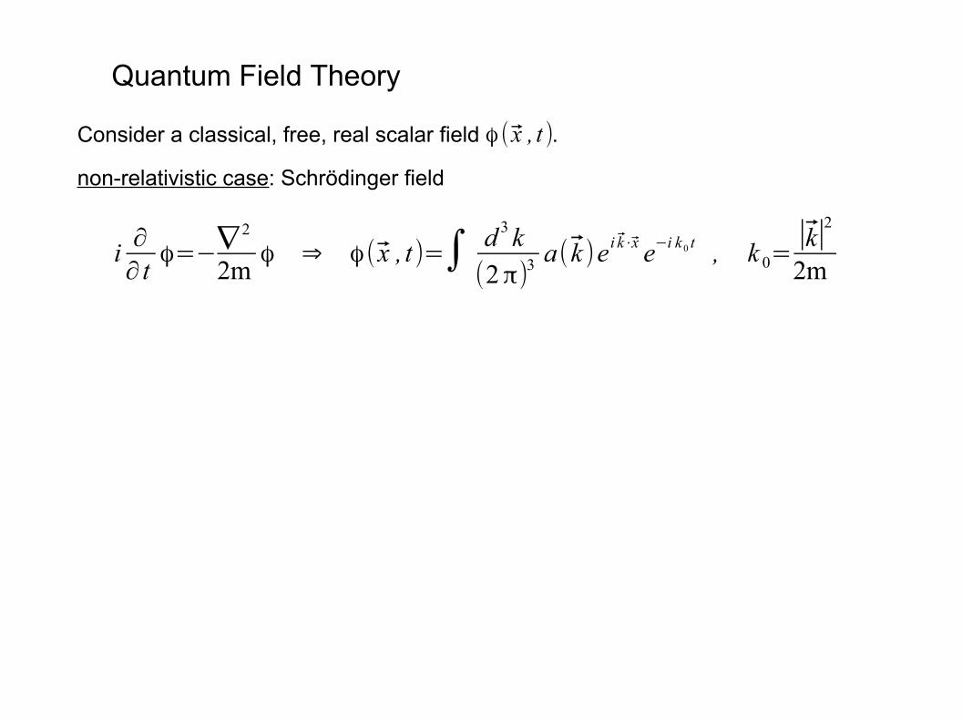
Consider a classical, free, real scalar field .
non-relativistic case: Schrödinger field
i∂∂ tϕ=−∇
2
2mϕ ⇒ ϕ( x , t)=∫ d 3 k
(2π)3a( k )ei k⋅x e−i k0 t , k 0=
∣k∣2
2m
ϕ( x , t )
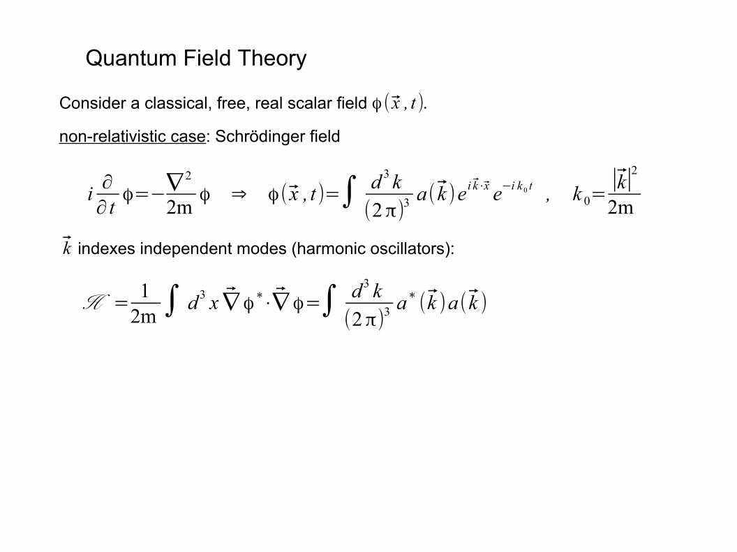
Quantum Field Theory
Consider a classical, free, real scalar field .
non-relativistic case: Schrödinger field
indexes independent modes (harmonic oscillators):
i∂∂ tϕ=−∇
2
2mϕ ⇒ ϕ( x , t)=∫ d 3 k
(2π)3a( k )ei k⋅x e−i k0 t , k 0=
∣k∣2
2m
ϕ( x , t )
H = 12m∫ d3 x ∇ ϕ∗⋅∇ ϕ=∫ d3 k
(2π)3a∗ (k )a( k )
k
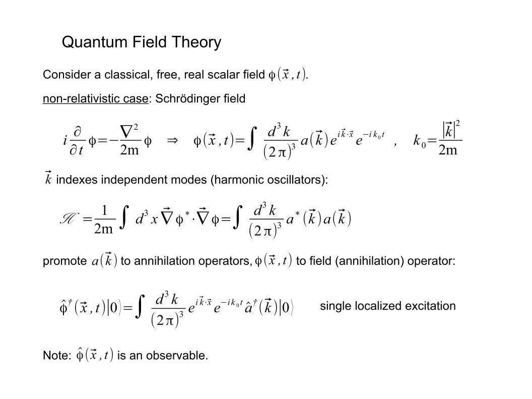
Quantum Field Theory
Consider a classical, free, real scalar field .
non-relativistic case: Schrödinger field
indexes independent modes (harmonic oscillators):
promote to annihilation operators, to field (annihilation) operator:
Note: is an observable.
i∂∂ tϕ=−∇
2
2mϕ ⇒ ϕ( x , t)=∫ d 3 k
(2π)3a( k )ei k⋅x e−i k0 t , k 0=
∣k∣2
2m
ϕ( x , t )
ϕ† ( x , t )∣0 ⟩=∫ d 3 k
(2π)3e i k⋅x e−i k 0 t a†( k )∣0 ⟩ single localized excitation
k
a( k ) ϕ( x , t )
ϕ( x , t )
H = 12m∫ d3 x ∇ ϕ∗⋅∇ ϕ=∫ d3 k
(2π)3a∗ (k )a( k )
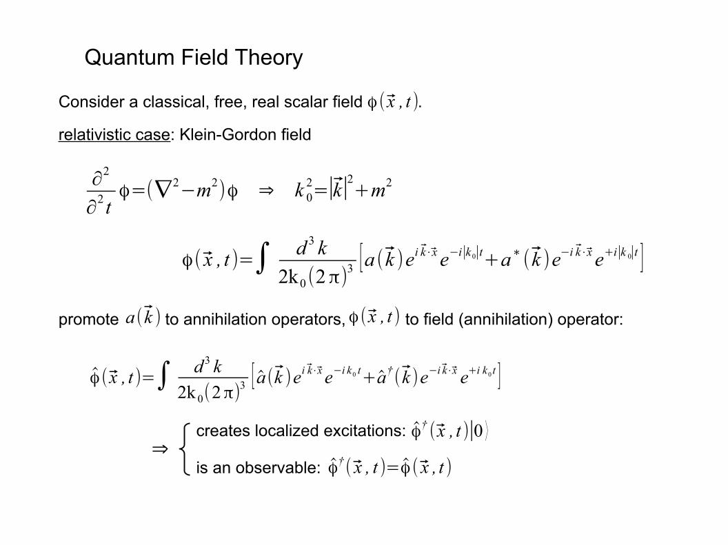
Quantum Field Theory
Consider a classical, free, real scalar field .
relativistic case: Klein-Gordon field
promote to annihilation operators, to field (annihilation) operator:
∂2
∂2 tϕ=(∇2−m2)ϕ ⇒ k 0
2=∣k∣2+m2
ϕ( x , t )=∫ d 3 k
2k0(2π)3 [a ( k )ei k⋅xe−i∣k0∣t+a∗ ( k )e−i k⋅xe+i∣k 0∣t ]
ϕ( x , t )
ϕ( x , t )=∫ d3 k
2k 0(2π)3 [ a(k )ei k⋅xe−i k0 t+a†( k )e−i k⋅x e+i k0 t ]
a( k ) ϕ( x , t )
ϕ† ( x , t )∣0 ⟩creates localized excitations:
is an observable: ϕ†( x , t )=ϕ( x , t )⇒
Quantum Field Theory
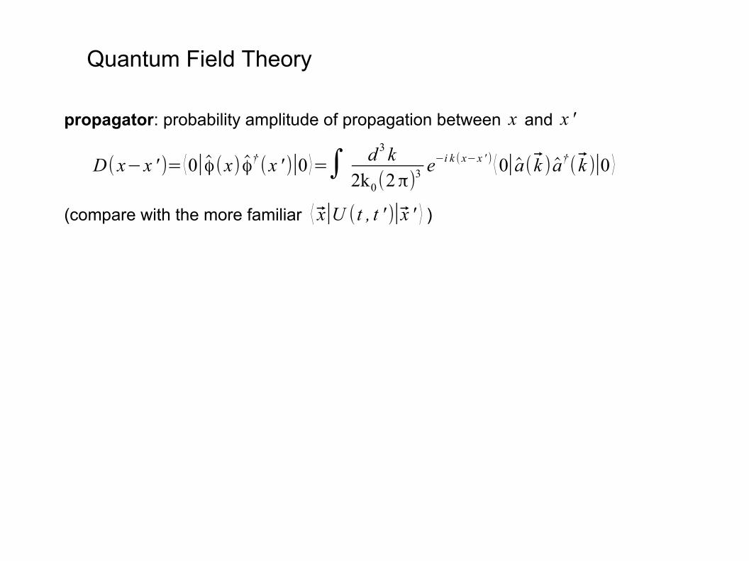
propagator: probability amplitude of propagation between and
(compare with the more familiar )
x x '
D( x−x ' )= ⟨0∣ϕ(x) ϕ† (x ' )∣0 ⟩=∫ d 3 k2k0(2π)
3 e−i k ( x−x ' ) ⟨0∣a( k ) a†( k )∣0 ⟩
⟨ x∣U (t , t ' )∣x ' ⟩
Quantum Field Theory
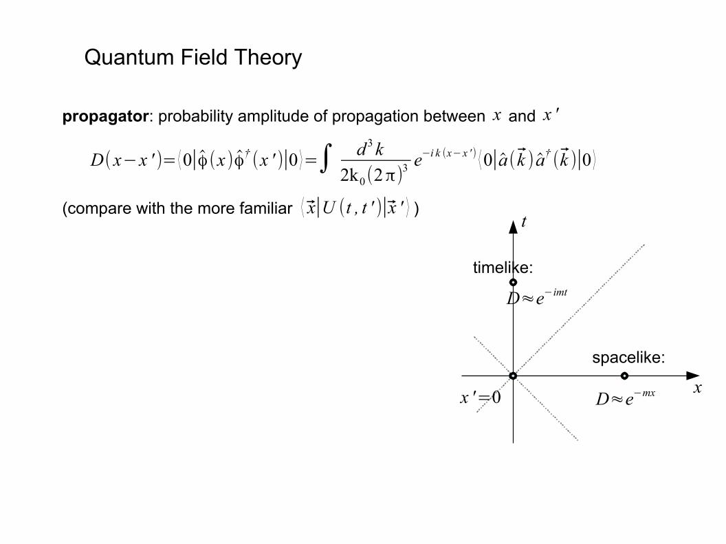
propagator: probability amplitude of propagation between and
(compare with the more familiar )
x x '
D(x−x ' )= ⟨0∣ϕ(x )ϕ† (x ' )∣0 ⟩=∫ d3k
2k0(2π)3 e−i k (x−x ' ) ⟨0∣a( k ) a† (k )∣0 ⟩
⟨ x∣U (t , t ' )∣x ' ⟩
x '=0x
t
D≈e−mx
D≈e−imt
spacelike:
timelike:
Quantum Field Theory
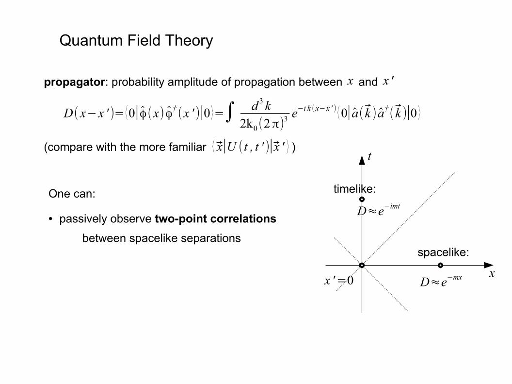
propagator: probability amplitude of propagation between and
(compare with the more familiar )
x x '
D( x−x ' )= ⟨0∣ϕ(x) ϕ† (x ' )∣0 ⟩=∫ d 3 k2k0(2π)
3 e−i k ( x−x ' ) ⟨0∣a( k ) a†( k )∣0 ⟩
⟨ x∣U (t , t ' )∣x ' ⟩
One can:
● passively observe two-point correlations
between spacelike separations
x '=0x
t
D≈e−mx
D≈e−imt
spacelike:
timelike:
Quantum Field Theory
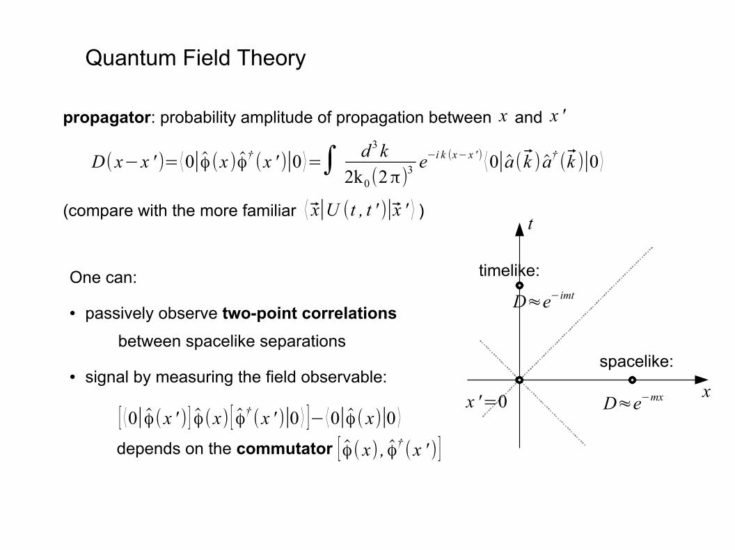
propagator: probability amplitude of propagation between and
(compare with the more familiar )
x x '
D(x−x ' )= ⟨0∣ϕ(x )ϕ† (x ' )∣0 ⟩=∫ d3k
2k0(2π)3 e−i k (x−x ' ) ⟨0∣a( k ) a† (k )∣0 ⟩
⟨ x∣U (t , t ' )∣x ' ⟩
One can:
● passively observe two-point correlations
between spacelike separations
● signal by measuring the field observable:
depends on the commutator [ ϕ( x) , ϕ† (x ' )]
x '=0x
t
D≈e−mx
D≈e−imt
spacelike:
timelike:
[ ⟨0∣ϕ(x ' )] ϕ(x) [ ϕ† (x ' )∣0 ⟩ ]− ⟨0∣ϕ( x)∣0 ⟩
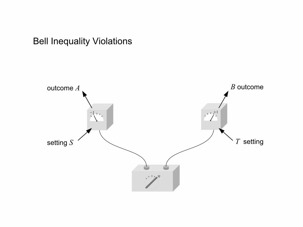
Bell Inequality Violations
ψ
+1−1
outcome A
setting S
B outcome
T setting
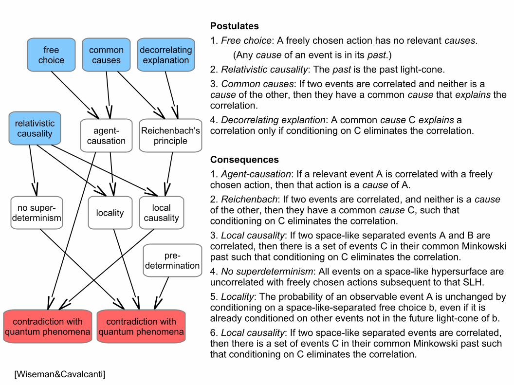
[Wiseman&Cavalcanti]
relativisticcausality
decorrelatingexplanation
commoncauses
freechoice
Postulates
1. Free choice: A freely chosen action has no relevant causes.
(Any cause of an event is in its past.)
2. Relativistic causality: The past is the past light-cone.
3. Common causes: If two events are correlated and neither is acause of the other, then they have a common cause that explains thecorrelation.
4. Decorrelating explantion: A common cause C explains acorrelation only if conditioning on C eliminates the correlation.
Consequences
1. Agent-causation: If a relevant event A is correlated with a freelychosen action, then that action is a cause of A.
2. Reichenbach: If two events are correlated, and neither is a cause of the other, then they have a common cause C, such thatconditioning on C eliminates the correlation.
3. Local causality: If two space-like separated events A and B arecorrelated, then there is a set of events C in their common Minkowskipast such that conditioning on C eliminates the correlation.
4. No superdeterminism: All events on a space-like hypersurface areuncorrelated with freely chosen actions subsequent to that SLH.
5. Locality: The probability of an observable event A is unchanged byconditioning on a space-like-separated free choice b, even if it isalready conditioned on other events not in the future light-cone of b.
6. Local causality: If two space-like separated events are correlated,then there is a set of events C in their common Minkowski past suchthat conditioning on C eliminates the correlation.
Reichenbach'sprinciple
agent-causation
no super-determinism locality
localcausality
contradiction withquantum phenomena
pre-determination
contradiction withquantum phenomena
[Wood&Spekkens]
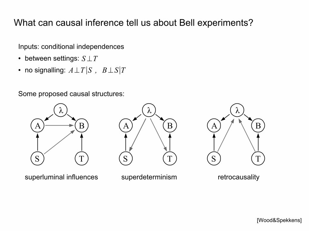
What can causal inference tell us about Bell experiments?
Inputs: conditional independences
● between settings:
● no signalling:
S⊥T
A⊥T∣S , B⊥S∣T
A
S
B
T
λ
A
S
B
T
λ
A
S
B
T
λ
superluminal influences superdeterminism retrocausality
Some proposed causal structures:
[Wood&Spekkens]
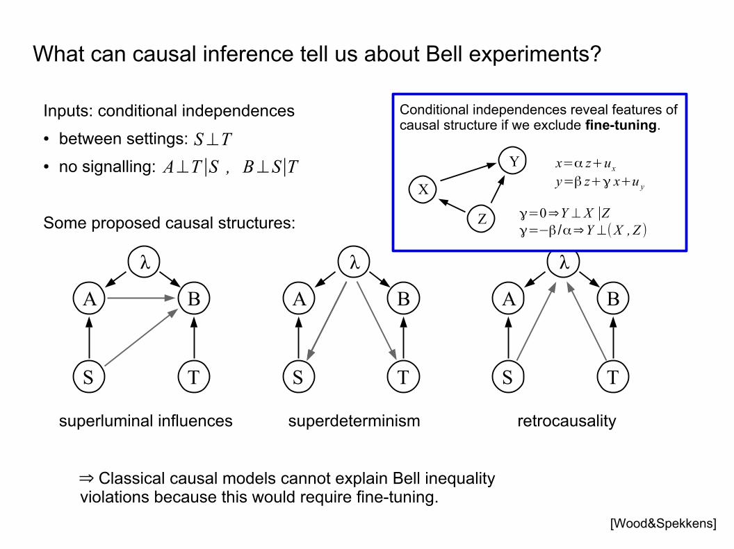
What can causal inference tell us about Bell experiments?
Inputs: conditional independences
● between settings:
● no signalling:
S⊥T
A⊥T∣S , B⊥S∣T
A
S
B
T
λ
A
S
B
T
λ
A
S
B
T
λ
superluminal influences superdeterminism retrocausality
Some proposed causal structures:
Conditional independences reveal features ofcausal structure if we exclude fine-tuning.
x=α z+ux
y=β z+γ x+u y
Z
X
Y
γ=0⇒Y ⊥ X ∣Zγ=−β/α⇒Y ⊥(X ,Z )
⇒ Classical causal models cannot explain Bell inequalityviolations because this would require fine-tuning.
Quantum Causal Models
How to describe causal relations between quantum systems?
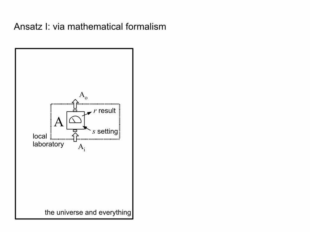
Ansatz I: via mathematical formalism
the universe and everything
locallaboratory
As setting
r result
Ai
Ao
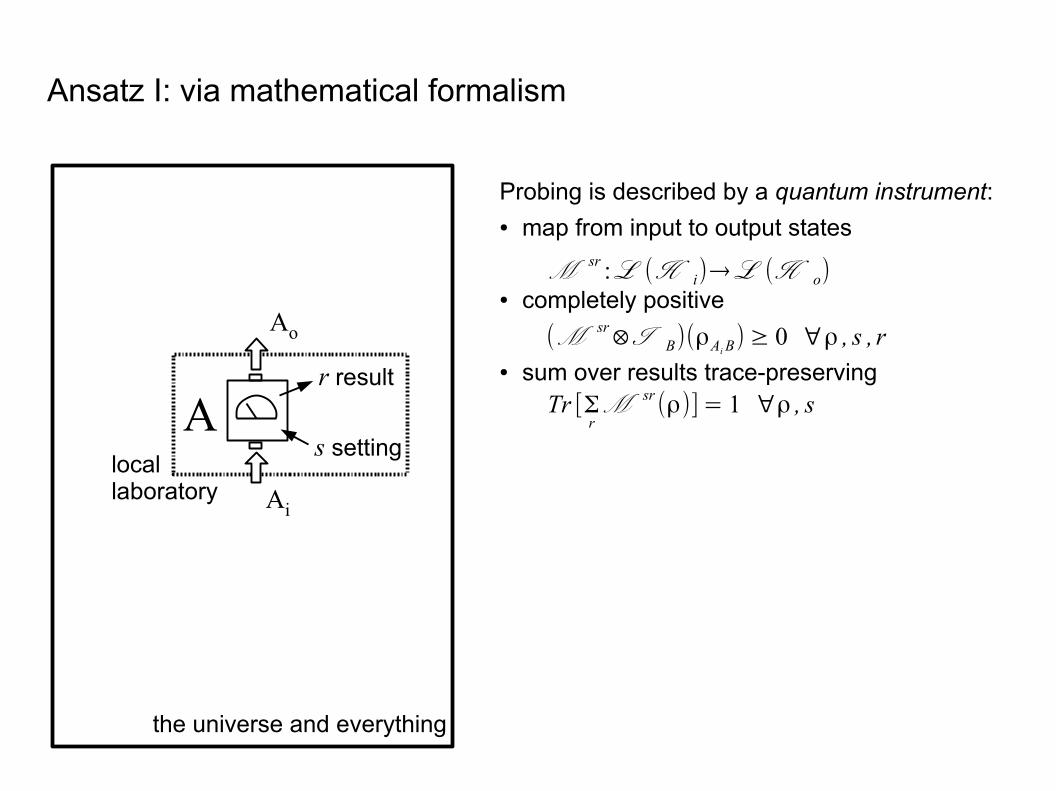
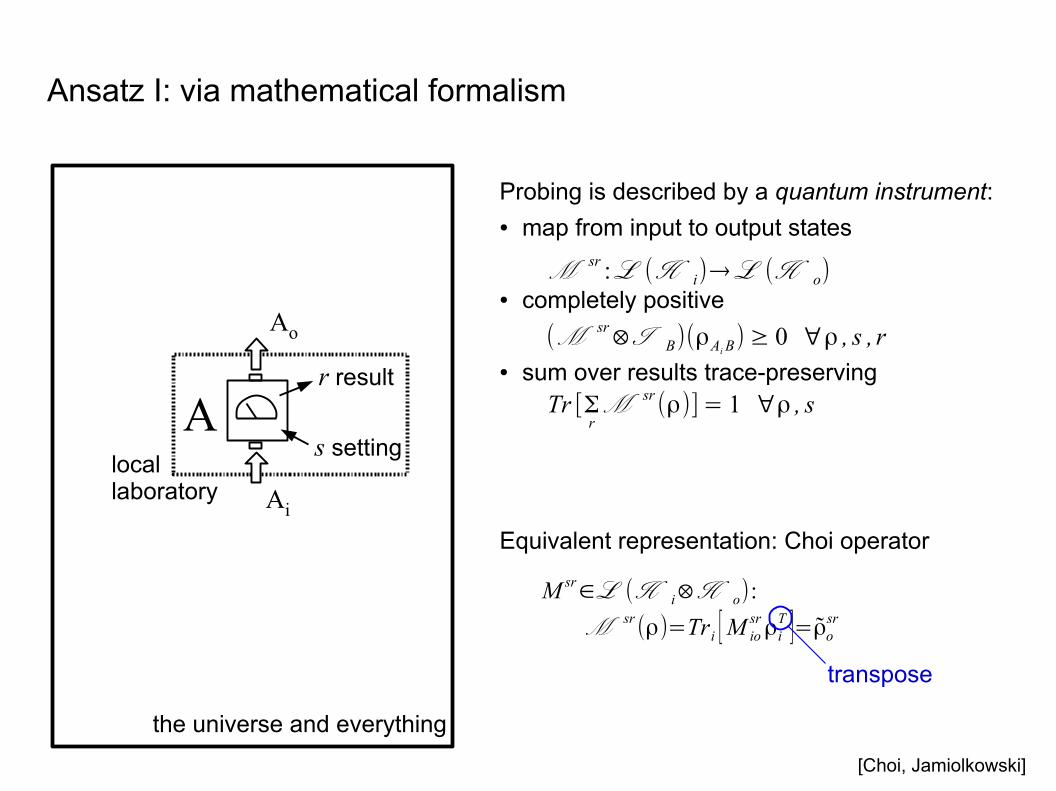
Ansatz I: via mathematical formalism
the universe and everything
locallaboratory
As setting
r result
Ai
Ao
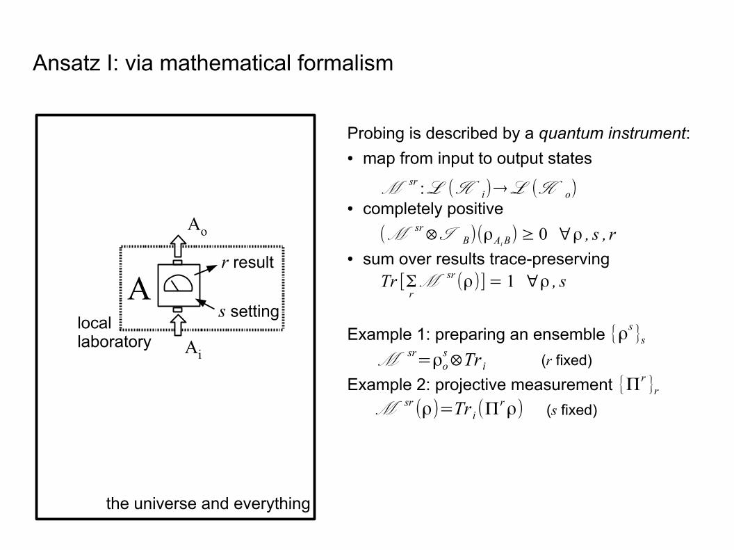
Probing is described by a quantum instrument:● map from input to output states
● completely positive
● sum over results trace-preserving
M sr :ℒ(H i)→ℒ (H o)
(M sr⊗I B)(ρAi B) ≥ 0 ∀ρ , s , r
Tr [ΣrM sr (ρ)] = 1 ∀ρ , s
Ansatz I: via mathematical formalism
the universe and everything
locallaboratory
As setting
r result
Ai
Ao
Probing is described by a quantum instrument:● map from input to output states
● completely positive
● sum over results trace-preserving
Example 1: preparing an ensemble
Example 2: projective measurement
M sr :ℒ(H i)→ℒ (H o)
(M sr⊗I B)(ρAi B) ≥ 0 ∀ρ , s , r
Tr [ΣrM sr (ρ)] = 1 ∀ρ , s
{ρs }sM sr=ρo
s⊗Tr i
{Πr }rM sr (ρ)=Tr i (Π
rρ)
(r fixed)
(s fixed)
Ansatz I: via mathematical formalism
the universe and everything
locallaboratory
As setting
r result
Ai
Ao
[Choi, Jamiolkowski]
Probing is described by a quantum instrument:● map from input to output states
● completely positive
● sum over results trace-preserving
Equivalent representation: Choi operator
M sr :ℒ(H i)→ℒ (H o)
(M sr⊗I B)(ρAi B) ≥ 0 ∀ρ , s , r
Tr [ΣrM sr (ρ)] = 1 ∀ρ , s
M sr∈ℒ(H i⊗H o):M sr(ρ)=Tri [M io
srρiT ]=ρo
sr
transpose
Ansatz I: via mathematical formalism
the universe and everything
locallaboratory
As setting
r result
Ai
Ao
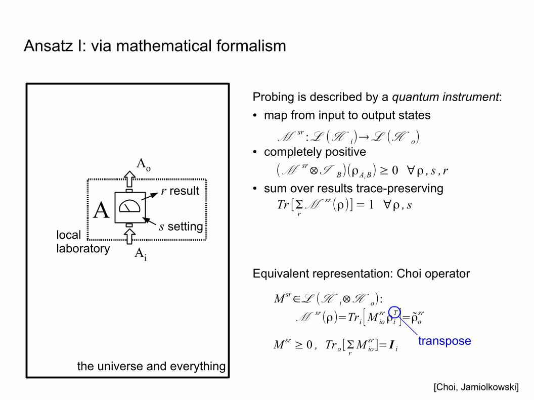
Probing is described by a quantum instrument:● map from input to output states
● completely positive
● sum over results trace-preserving
Equivalent representation: Choi operator
M sr :ℒ(H i)→ℒ (H o)
(M sr⊗I B)(ρAi B) ≥ 0 ∀ρ , s , r
Tr [ΣrM sr (ρ)] = 1 ∀ρ , s
M sr∈ℒ(H i⊗H o):M sr(ρ)=Tri [M io
srρiT ]=ρo
sr
M sr ≥ 0 , Tr o [ΣrM io
sr ]= I itranspose
[Choi, Jamiolkowski]
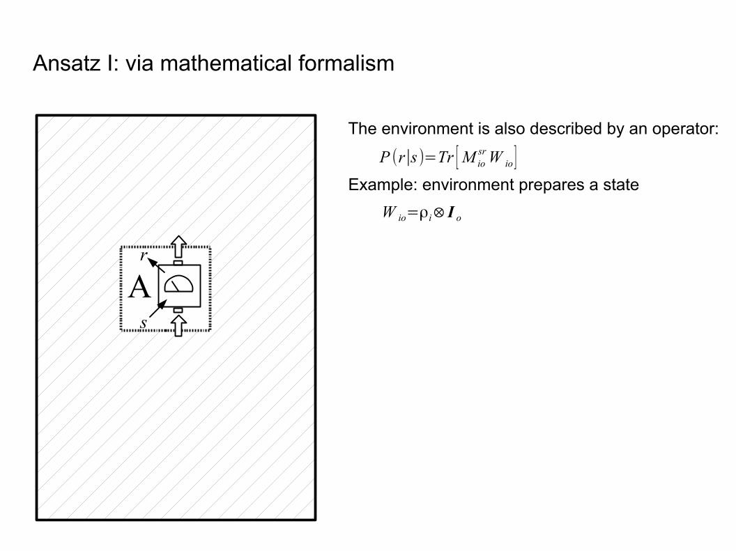
The environment is also described by an operator:
Example: environment prepares a state
Ansatz I: via mathematical formalism
P (r∣s)=Tr [M iosrW io ]
As
r
W io=ρi⊗ I o
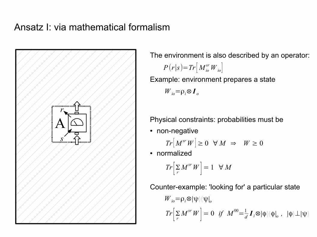
The environment is also described by an operator:
Example: environment prepares a state
Physical constraints: probabilities must be● non-negative
● normalized
Counter-example: 'looking for' a particular state
Ansatz I: via mathematical formalism
P (r∣s)=Tr [M iosrW io ]
Tr [M srW ]≥ 0 ∀M ⇒ W ≥ 0
Tr [Σr M srW ]= 1 ∀M
As
r
W io=ρi⊗ I o
W io=ρi⊗∣ψ ⟩ ⟨ψ∣o
Tr [Σr M srW ]= 0 if M 00=1dI i⊗∣ϕ ⟩ ⟨ϕ∣o , ∣ϕ ⟩⊥∣ψ ⟩
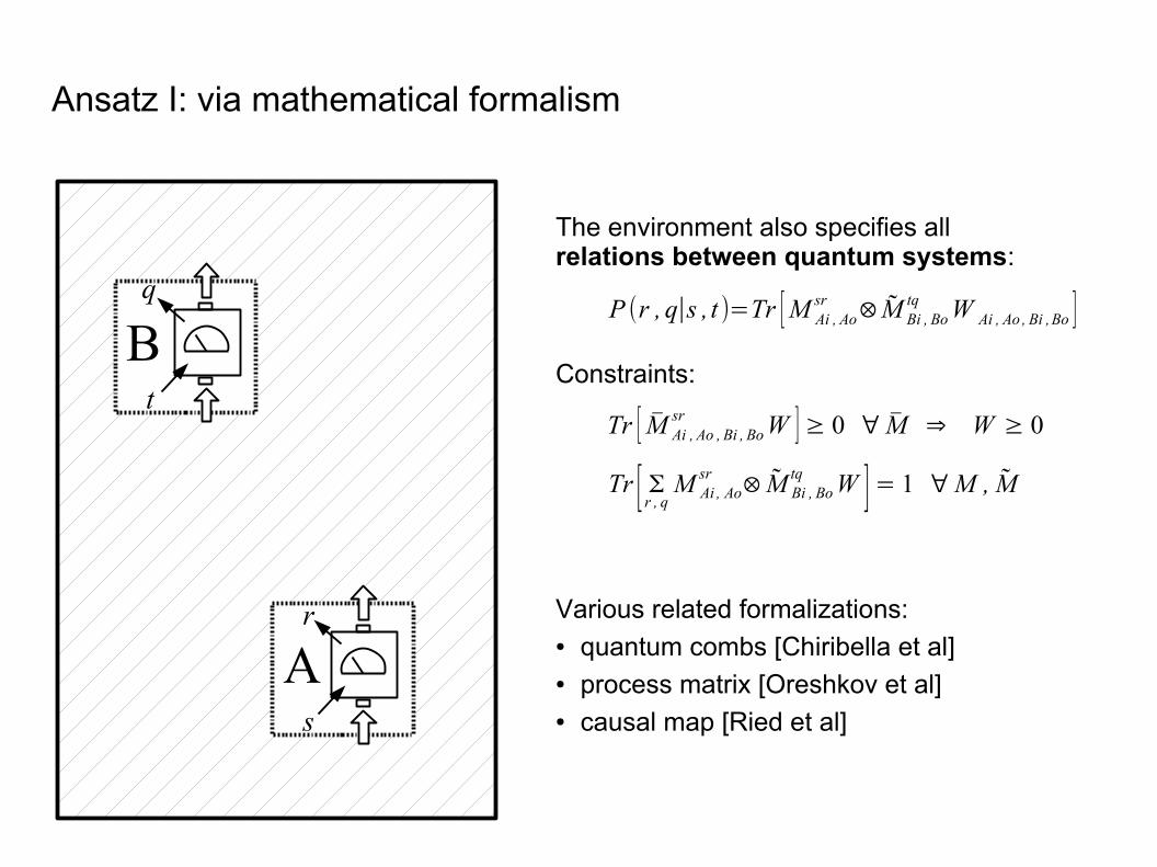
The environment also specifies allrelations between quantum systems:
Constraints:
Various related formalizations:● quantum combs [Chiribella et al]● process matrix [Oreshkov et al]● causal map [Ried et al]
Ansatz I: via mathematical formalism
P (r , q∣s , t )=Tr [M Ai , Aosr ⊗M Bi , Bo
tq W Ai , Ao , Bi ,Bo ]
Tr [ M Ai , Ao , Bi , Bosr W ]≥ 0 ∀ M ⇒ W ≥ 0
Tr [ Σr , q M Ai , Aosr ⊗M Bi , Bo
tq W ]= 1 ∀M , M
As
r
Bt
q
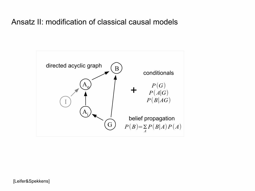
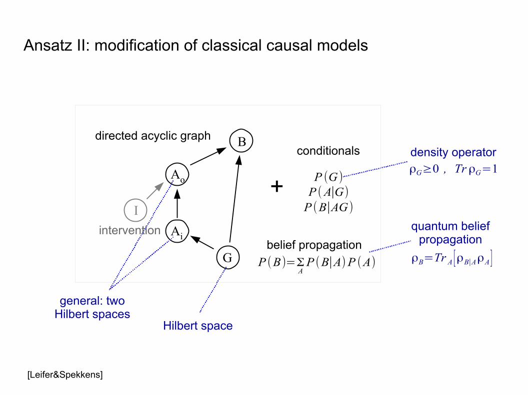
Ansatz II: modification of classical causal models
directed acyclic graphconditionals
+P (G)
P (A∣G)P (B∣AG)
G
Ai
B
Ao
I
P (B)=ΣAP (B∣A)P (A)
belief propagation
[Leifer&Spekkens]
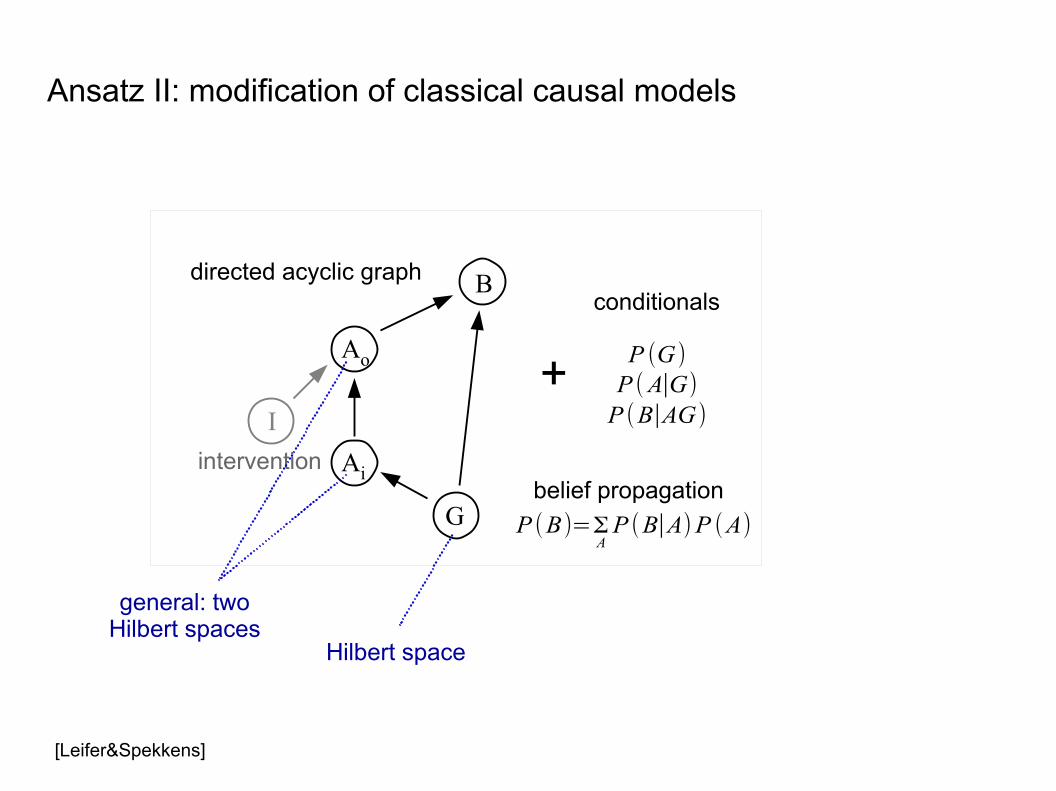
Ansatz II: modification of classical causal models
directed acyclic graphconditionals
+P (G)
P (A∣G)P (B∣AG)
G
Ai
B
Ao
I
intervention
Hilbert space
general: twoHilbert spaces
P (B)=ΣAP (B∣A)P (A)
belief propagation
[Leifer&Spekkens]
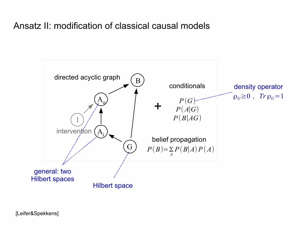
Ansatz II: modification of classical causal models
directed acyclic graphconditionals
+P (G)
P (A∣G)P (B∣AG)
G
Ai
B
Ao
I
intervention
Hilbert space
ρG≥0 , Tr ρG=1density operator
general: twoHilbert spaces
P (B)=ΣAP (B∣A)P (A)
belief propagation
[Leifer&Spekkens]
Ansatz II: modification of classical causal models
directed acyclic graphconditionals
+P (G)
P (A∣G)P (B∣AG)
G
Ai
B
Ao
I
intervention
Hilbert space
ρG≥0 , Tr ρG=1density operator
general: twoHilbert spaces
P (B)=ΣAP (B∣A)P (A)
belief propagationρB=Tr A [ρB∣AρA ]
quantum beliefpropagation
[Leifer&Spekkens]
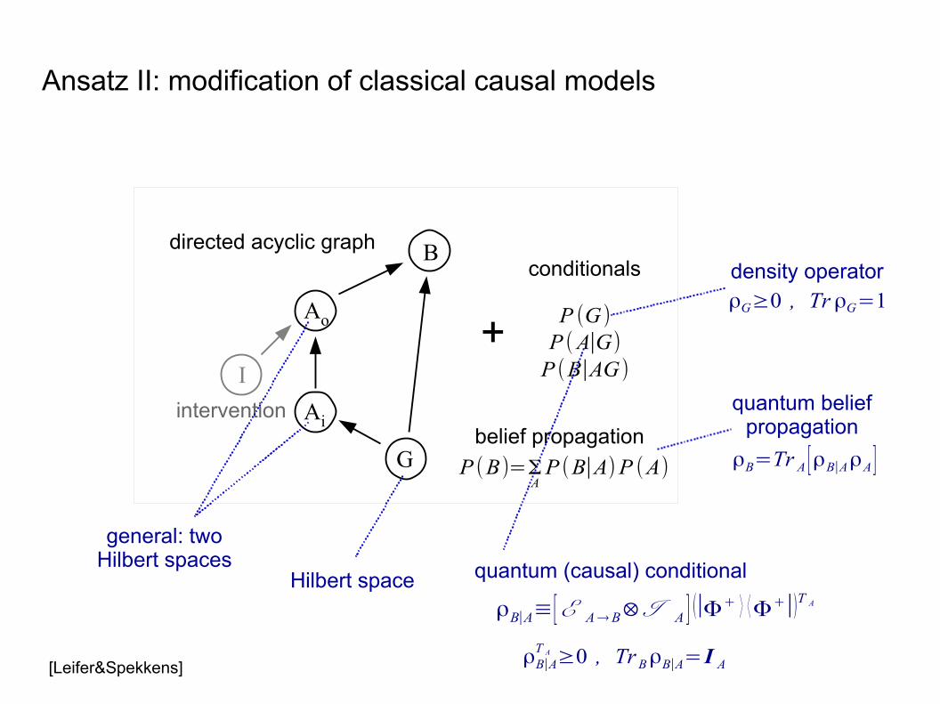
Ansatz II: modification of classical causal models
directed acyclic graphconditionals
+P (G)
P (A∣G)P (B∣AG)
G
Ai
B
Ao
I
intervention
Hilbert space
ρG≥0 , Tr ρG=1density operator
general: twoHilbert spaces
P (B)=ΣAP (B∣A)P (A)
belief propagationρB=Tr A [ρB∣AρA ]
quantum beliefpropagation
quantum (causal) conditional
ρB∣A≡[E A→B⊗I A ] (∣Φ+ ⟩ ⟨Φ+∣)T A
ρB∣AT A ≥0 , Tr BρB∣A=I A[Leifer&Spekkens]
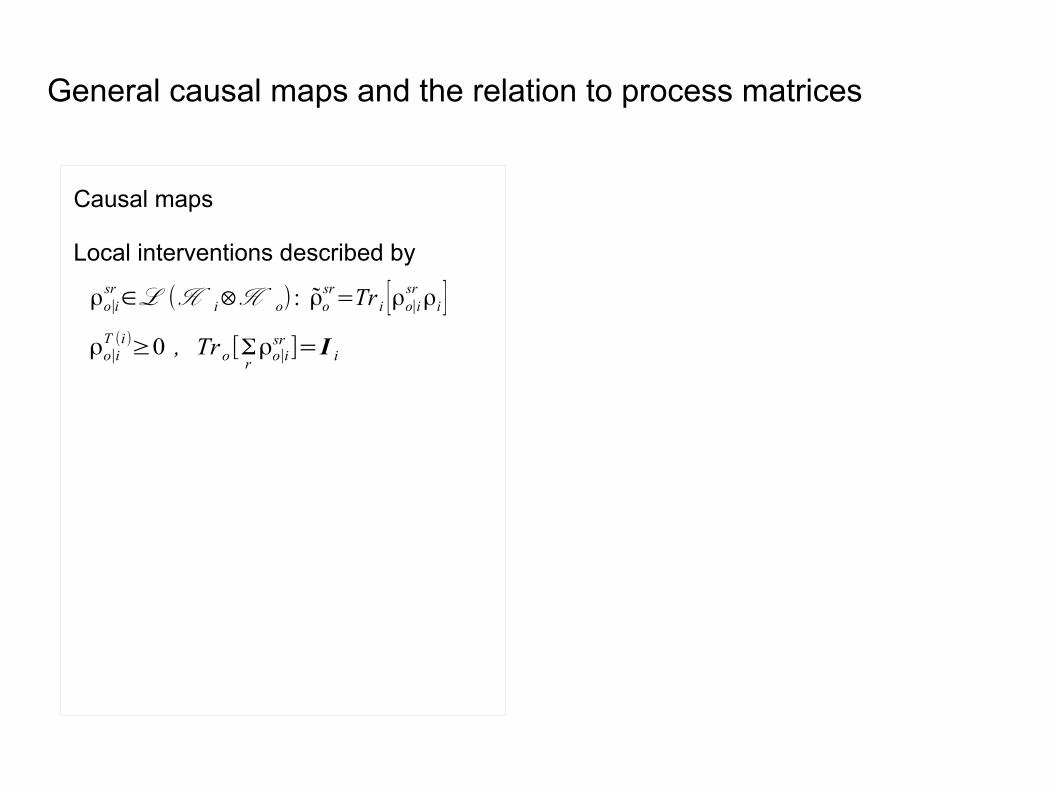
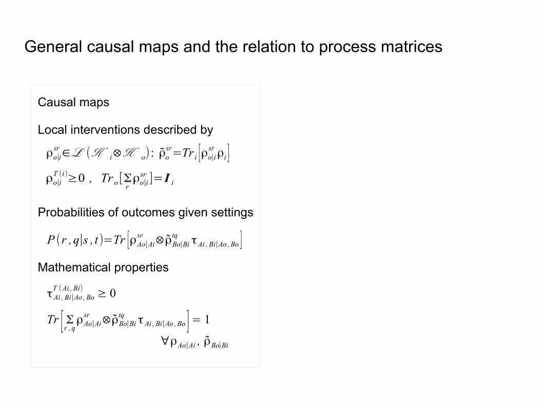
General causal maps and the relation to process matrices
Causal maps
Local interventions described by
ρo∣iT (i)≥0 , Tro [Σ
rρo∣i
sr ]=I i
ρo∣isr∈ℒ(H i⊗H o) : ρo
sr=Tr i [ρo∣isr ρi ]
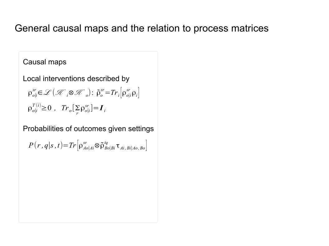
General causal maps and the relation to process matrices
Causal maps
Local interventions described by
Probabilities of outcomes given settings
ρo∣iT (i)≥0 , Tro [Σ
rρo∣i
sr ]=I i
ρo∣isr∈ℒ(H i⊗H o) : ρo
sr=Tr i [ρo∣isr ρi ]
P (r ,q∣s , t )=Tr [ρAo∣Aisr ⊗ρBo∣Bi
tq τAi , Bi∣Ao , Bo ]
General causal maps and the relation to process matrices
Causal maps
Local interventions described by
Probabilities of outcomes given settings
Mathematical properties
ρo∣iT (i)≥0 , Tro [Σ
rρo∣i
sr ]=I i
ρo∣isr∈ℒ(H i⊗H o) : ρo
sr=Tr i [ρo∣isr ρi ]
P (r ,q∣s , t )=Tr [ρAo∣Aisr ⊗ρBo∣Bi
tq τAi , Bi∣Ao , Bo ]
τAi , Bi∣Ao , BoT (Ai , Bi) ≥ 0
Tr [ Σr ,qρAo∣Ai
sr ⊗ρBo∣Bitq τAi , Bi∣Ao , Bo ]= 1
∀ρAo∣Ai , ρBo∣Bi
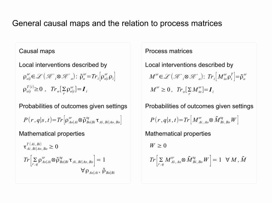
P (r ,q∣s , t )=Tr [M Ai , Aosr ⊗M Bi , Bo
tq W ]
W ≥ 0
Tr [ Σr ,qM Ai , Ao
sr ⊗M Bi , Botq W ]= 1 ∀M , M
M sr∈ℒ(H i⊗H o): Tr i [M iosrρi
T ]=ρosr
M sr ≥ 0 , Tr o [ΣrM io
sr ]= I i
Process matrices
Local interventions described by
Probabilities of outcomes given settings
Mathematical properties
[Leifer&Spekkens]
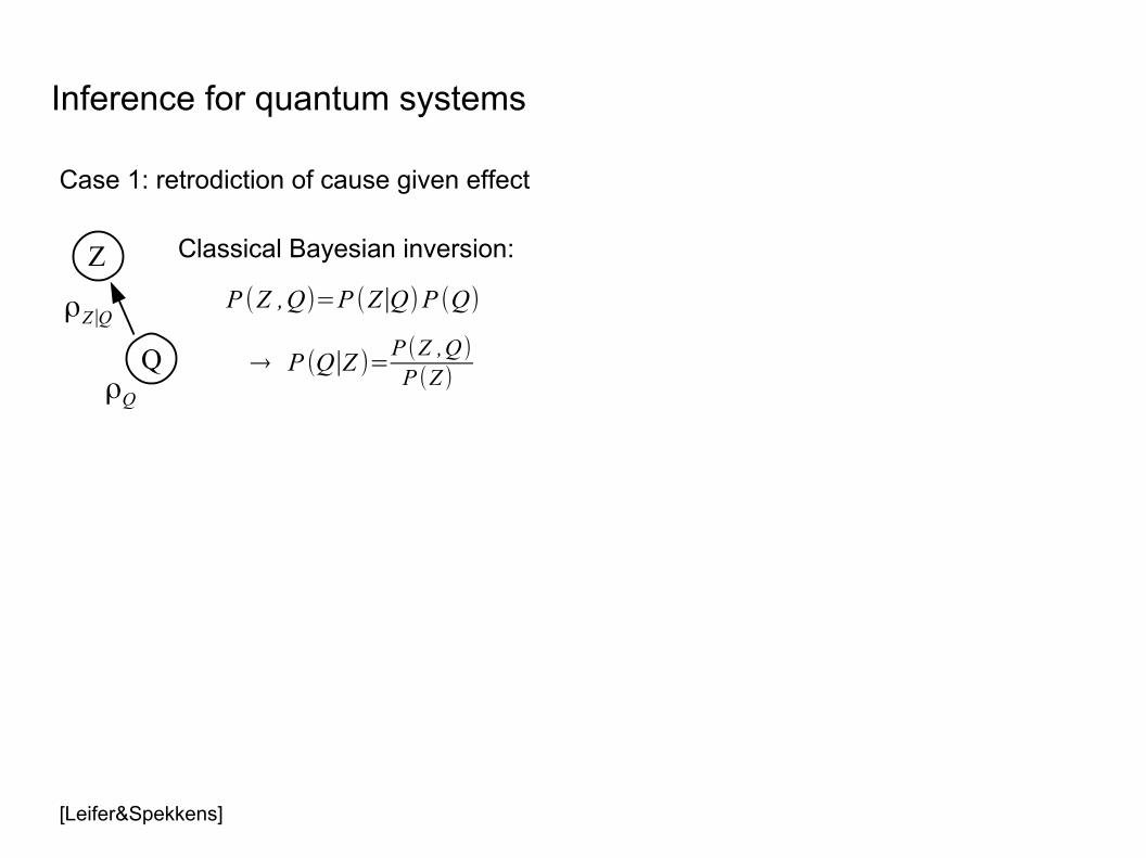
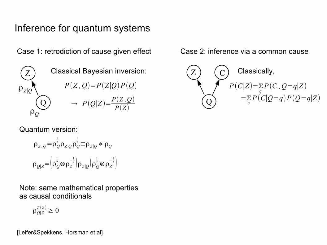
Inference for quantum systems
Case 1: retrodiction of cause given effect
P (Z ,Q)=P (Z∣Q)P (Q)
→ P (Q∣Z )=P (Z ,Q)P (Z )
Classical Bayesian inversion:
Q
Z
ρQ
ρZ∣Q
[Leifer&Spekkens, Horsman et al]
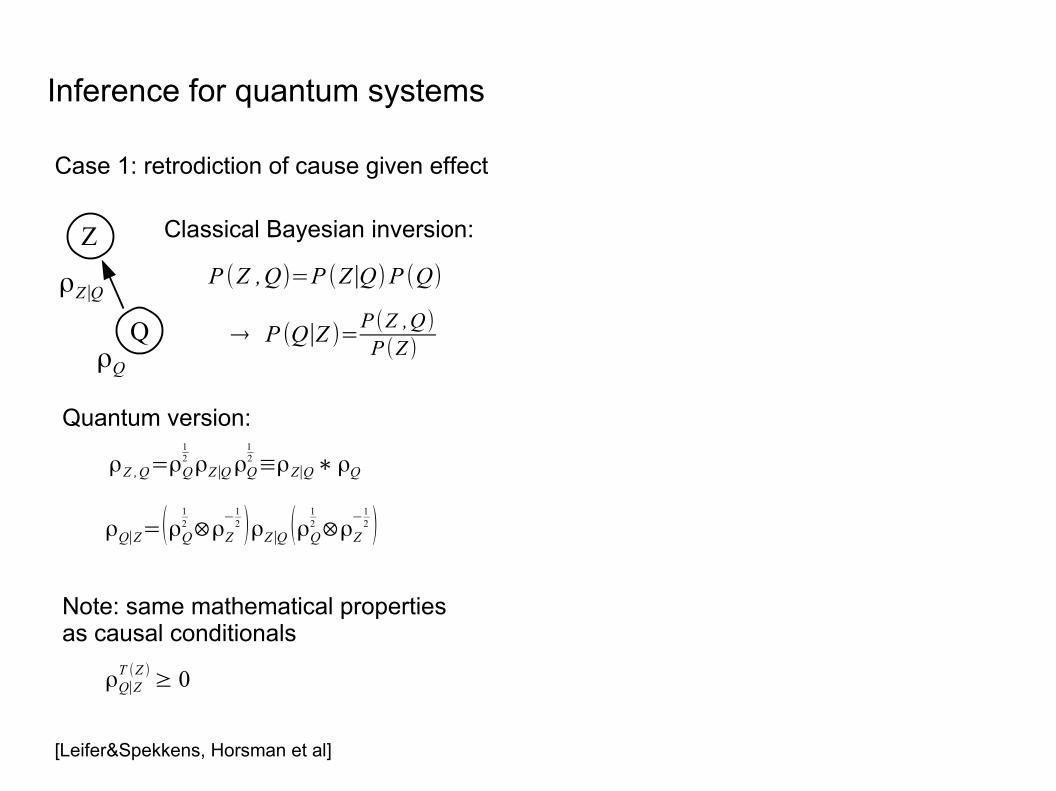
Inference for quantum systems
Case 1: retrodiction of cause given effect
P (Z ,Q)=P (Z∣Q)P (Q)
→ P (Q∣Z )=P (Z ,Q)P (Z )
Classical Bayesian inversion:
Q
Z
Quantum version:
ρQ
ρZ∣Q
ρQ∣Z=(ρQ
12 ⊗ρZ
−12 )ρZ∣Q (ρQ
12 ⊗ρZ
−12 )
Note: same mathematical propertiesas causal conditionals
ρQ∣ZT (Z )≥ 0
ρZ ,Q=ρQ
12 ρZ∣QρQ
12 ≡ρZ∣Q∗ρQ
Inference for quantum systems
Case 1: retrodiction of cause given effect
P (Z ,Q)=P (Z∣Q)P (Q)
→ P (Q∣Z )=P (Z ,Q)P (Z )
Classical Bayesian inversion:
Q
Z
Q
Z C
Case 2: inference via a common cause
P (C∣Z )=ΣqP (C ,Q=q∣Z )
=ΣqP (C∣Q=q)P (Q=q∣Z )
Quantum version:
ρQ
ρZ∣Q
ρQ∣Z=(ρQ
12 ⊗ρZ
−12 )ρZ∣Q (ρQ
12 ⊗ρZ
−12 )
Classically,
Note: same mathematical propertiesas causal conditionals
ρQ∣ZT (Z )≥ 0
ρZ ,Q=ρQ
12 ρZ∣QρQ
12 ≡ρZ∣Q∗ρQ
[Leifer&Spekkens, Horsman et al]
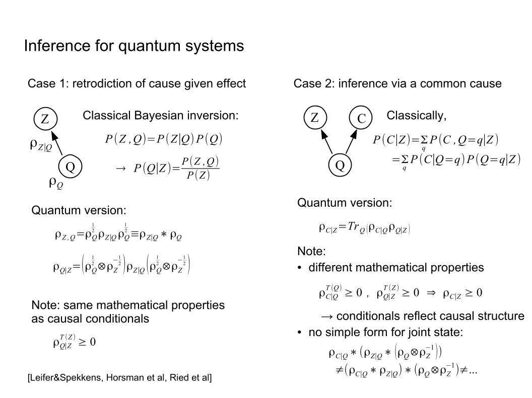
Inference for quantum systems
Case 1: retrodiction of cause given effect
P (Z ,Q)=P (Z∣Q)P (Q)
→ P (Q∣Z )=P (Z ,Q)P (Z )
Classical Bayesian inversion:
Q
Z
Q
Z C
Case 2: inference via a common cause
P (C∣Z )=ΣqP (C ,Q=q∣Z )
=ΣqP (C∣Q=q)P (Q=q∣Z )
Quantum version:
ρQ
ρZ∣Q
ρZ ,Q=ρQ
12 ρZ∣QρQ
12 ≡ρZ∣Q∗ρQ
ρQ∣Z=(ρQ
12 ⊗ρZ
−12 )ρZ∣Q (ρQ
12 ⊗ρZ
−12 )
Classically,
ρC∣Z=TrQ (ρC∣QρQ∣Z )
Note: same mathematical propertiesas causal conditionals
ρQ∣ZT (Z )≥ 0
Quantum version:
Note:● different mathematical properties
→ conditionals reflect causal structure● no simple form for joint state:
ρC∣QT (Q)≥ 0 , ρQ∣Z
T (Z )≥ 0 ⇒ ρC∣Z ≥ 0
ρC∣Q∗(ρZ∣Q∗ (ρQ⊗ρZ−1 ))
≠(ρC∣Q∗ρZ∣Q)∗ (ρQ⊗ρZ−1)≠...
[Leifer&Spekkens, Horsman et al, Ried et al]
Causal Structure in a Quantum World
Given an operator relating several quantum systems,
● Can it be decomposed into separate causal relations?
● What kinds of causal relations can there be?
● How to classify the possible causal relations?
Causal Structure in a Quantum World
Causal Loops
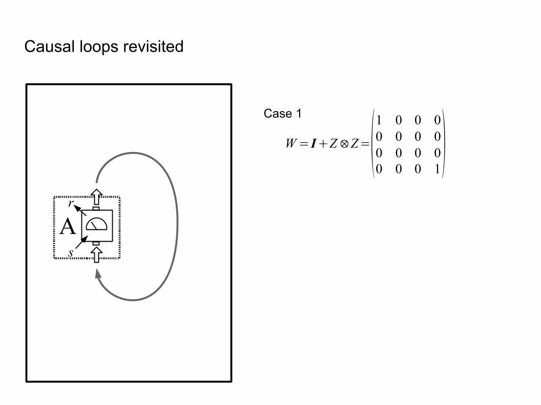
Case 1
W=I+Z⊗Z=(1 0 0 00 0 0 00 0 0 00 0 0 1
)
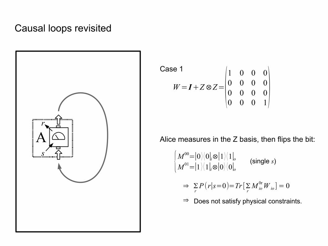
Causal loops revisited
As
r
Case 1
Alice measures in the Z basis, then flips the bit:
W=I+Z⊗Z=(1 0 0 00 0 0 00 0 0 00 0 0 1
)
Causal loops revisited
{M 00=∣0 ⟩ ⟨0∣i⊗∣1 ⟩ ⟨1∣oM 01=∣1 ⟩ ⟨1∣i⊗∣0 ⟩ ⟨0∣o
⇒ ΣrP (r∣s=0)=Tr [Σ
rM io
0rW io ] = 0
(single s)
Does not satisfy physical constraints.
As
r
⇒
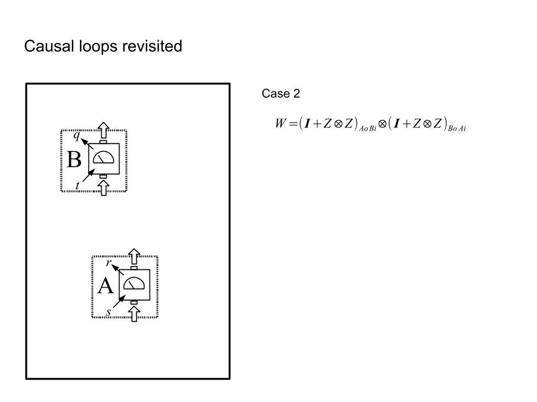
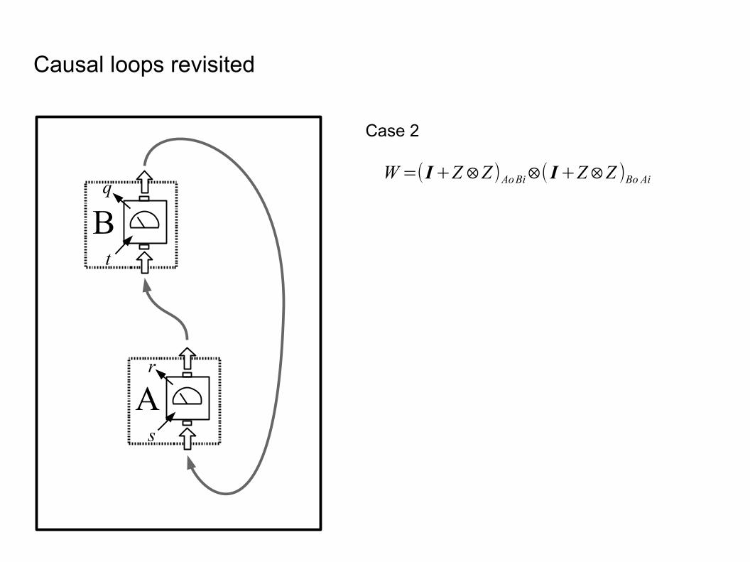
Case 2
W=(I+Z⊗Z )AoBi⊗( I+Z⊗Z )Bo Ai
Causal loops revisited
As
r
Bt
q
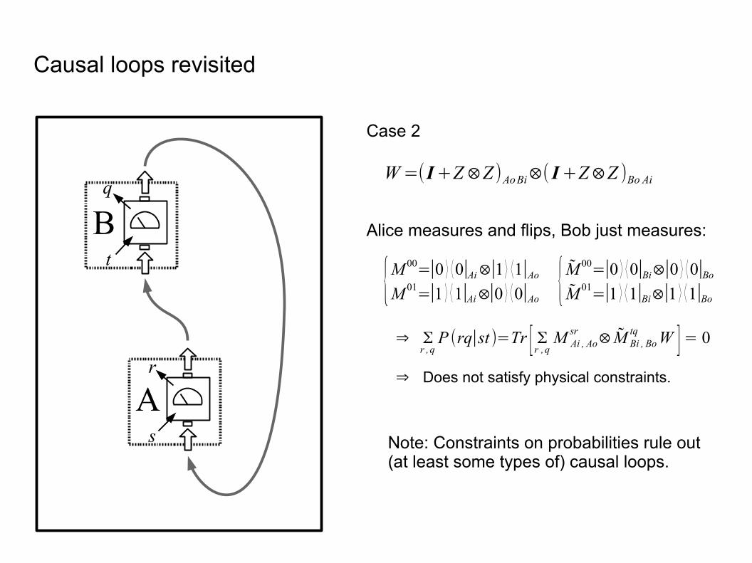
Case 2
W=(I+Z⊗Z )AoBi⊗( I+Z⊗Z )Bo Ai
Causal loops revisited
As
r
Bt
q
Case 2
Note: Constraints on probabilities rule out(at least some types of) causal loops.
W=(I+Z⊗Z )AoBi⊗( I+Z⊗Z )Bo Ai
Causal loops revisited
Alice measures and flips, Bob just measures:
{M 00=∣0 ⟩ ⟨0∣Ai⊗∣1 ⟩ ⟨1∣Ao
M 01=∣1 ⟩ ⟨1∣Ai⊗∣0 ⟩ ⟨0∣Ao
As
r
Bt
q
{M 00=∣0 ⟩ ⟨0∣Bi⊗∣0 ⟩ ⟨0∣Bo
M 01=∣1 ⟩ ⟨1∣Bi⊗∣1 ⟩ ⟨1∣Bo
⇒ Σr ,q
P (rq∣st )=Tr [ Σr ,qM Ai , Ao
sr ⊗M Bi , Botq W ]= 0
⇒ Does not satisfy physical constraints.
Case 3
Causal loops revisited
W= 12W B<A+
12W A<B
= 18 ( I+ 1
√2Z Bo⊗Z Ai )+ 1
8 ( I+ 1
√2Z Bi⊗X A1
⊗Z Ao)
As
r
Bt
q
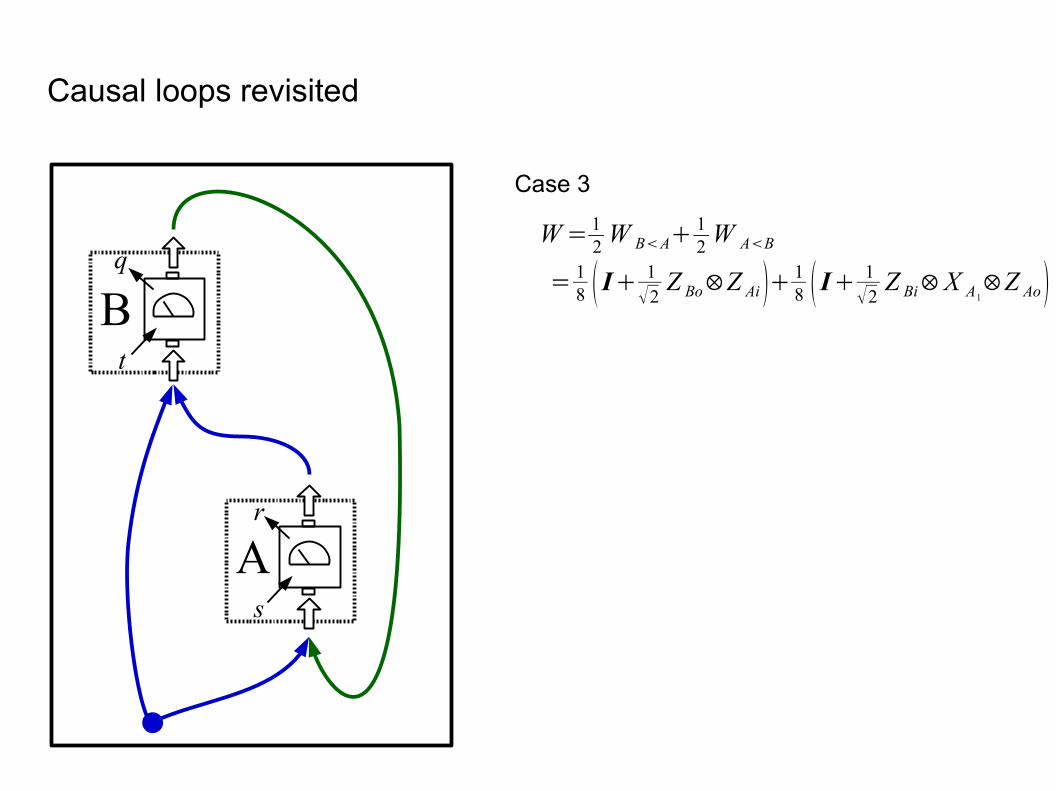
Case 3
Causal loops revisited
W= 12W B<A+
12W A<B
= 18 ( I+ 1
√2Z Bo⊗Z Ai )+ 1
8 ( I+ 1
√2Z Bi⊗X A1
⊗Z Ao)
λ B<A=14 (1± 1
√2 ) ; λA<B=14 (1± 1
√2 )check positivity:
As
r
Bt
q
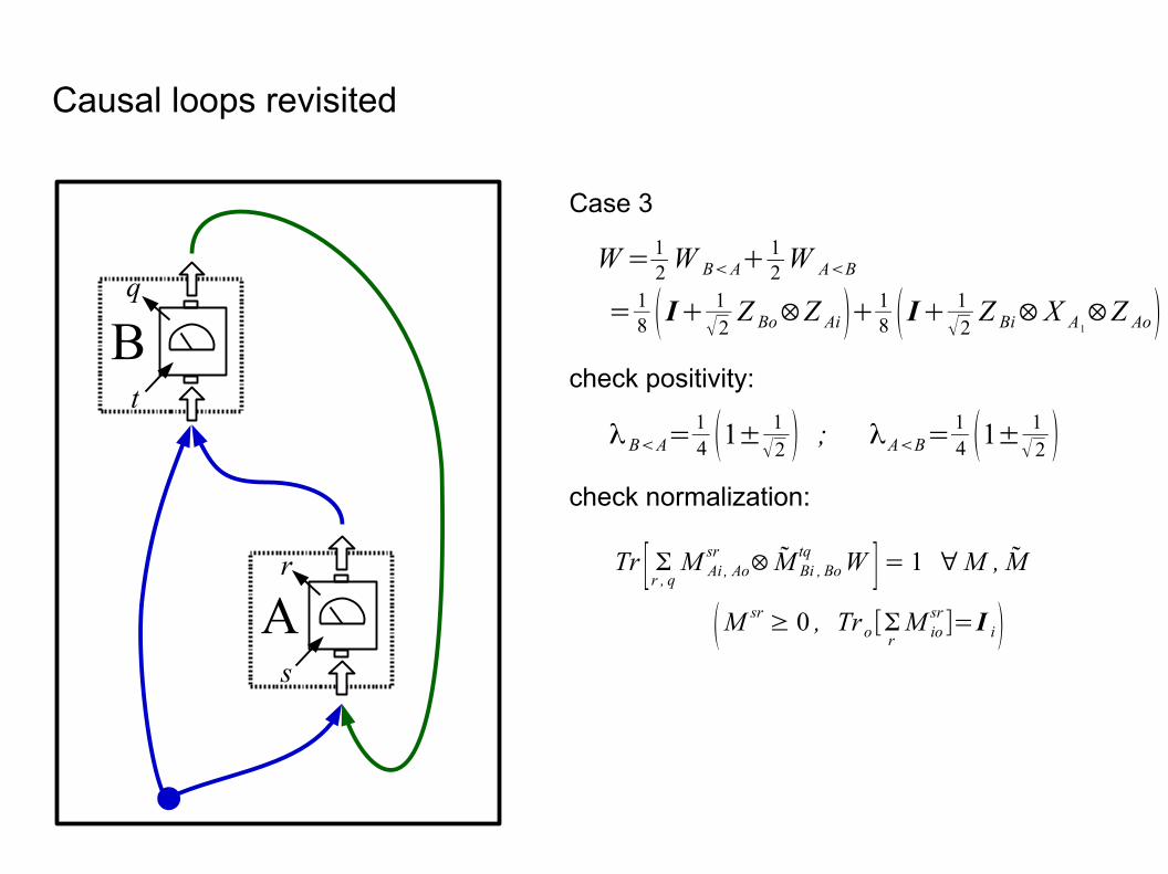
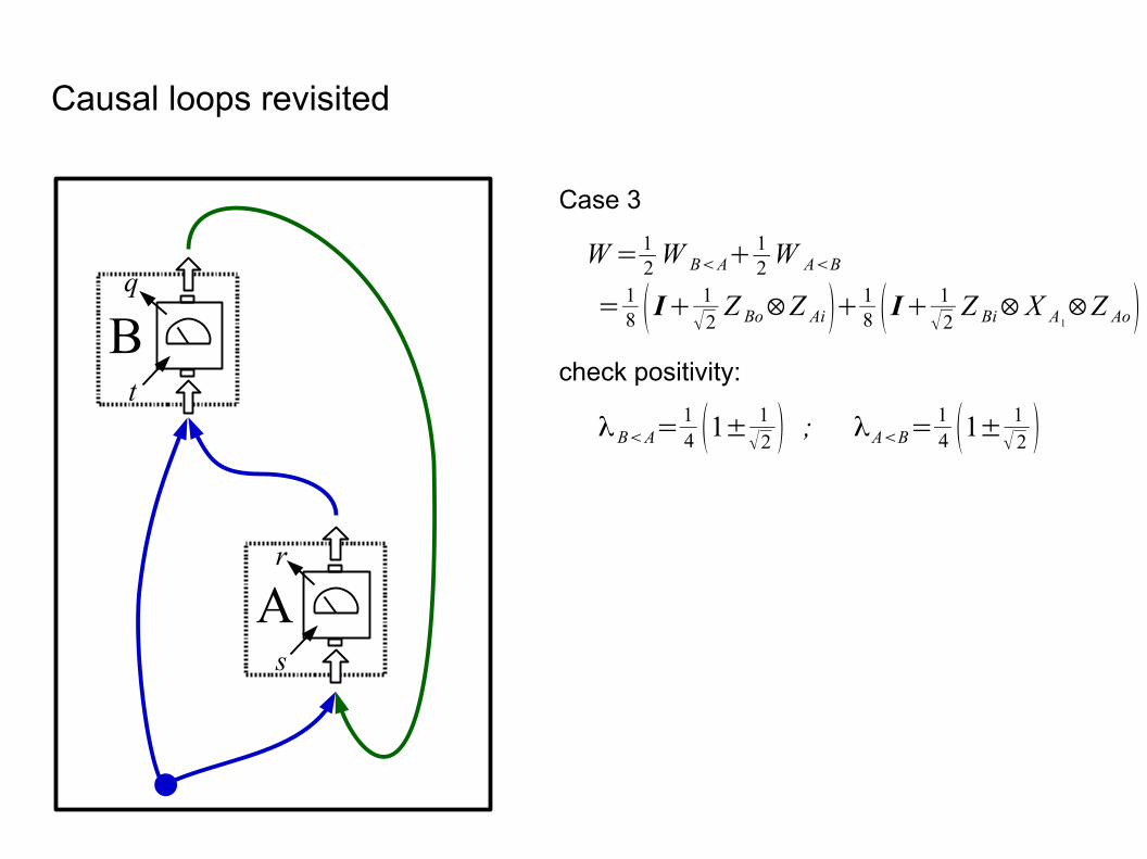
Case 3
Causal loops revisited
W= 12W B<A+
12W A<B
= 18 ( I+ 1
√2Z Bo⊗Z Ai )+ 1
8 ( I+ 1
√2Z Bi⊗X A1
⊗Z Ao)
λ B<A=14 (1± 1
√2 ) ; λA<B=14 (1± 1
√2 )check positivity:
check normalization:
As
r
Bt
q
Tr [ Σr , q M Ai , Aosr ⊗M Bi , Bo
tq W ]= 1 ∀M , M
(M sr ≥ 0 , Tro [Σr M iosr ]=I i )
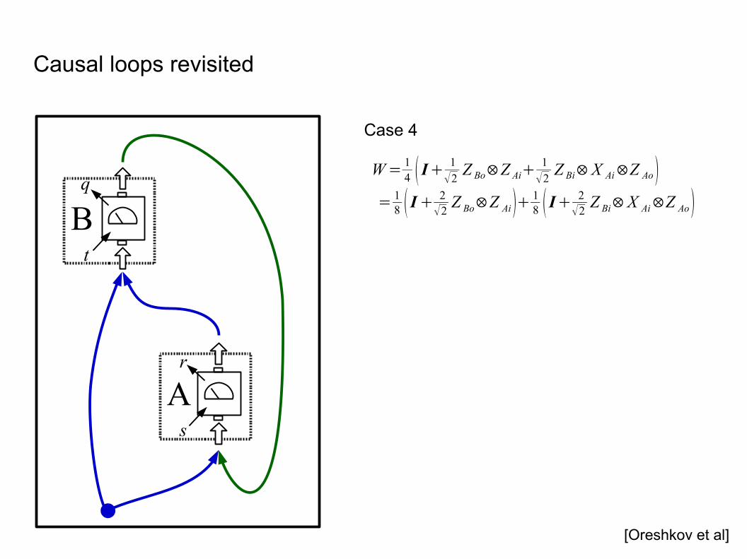
Case 4
[Oreshkov et al]
W= 14 ( I+ 1
√2Z Bo⊗Z Ai+
1
√2Z Bi⊗X Ai⊗Z Ao )
= 18 ( I+ 2
√2Z Bo⊗Z Ai )+ 1
8 ( I+ 2√2
Z Bi⊗X Ai⊗Z Ao )
Causal loops revisited
As
r
Bt
q
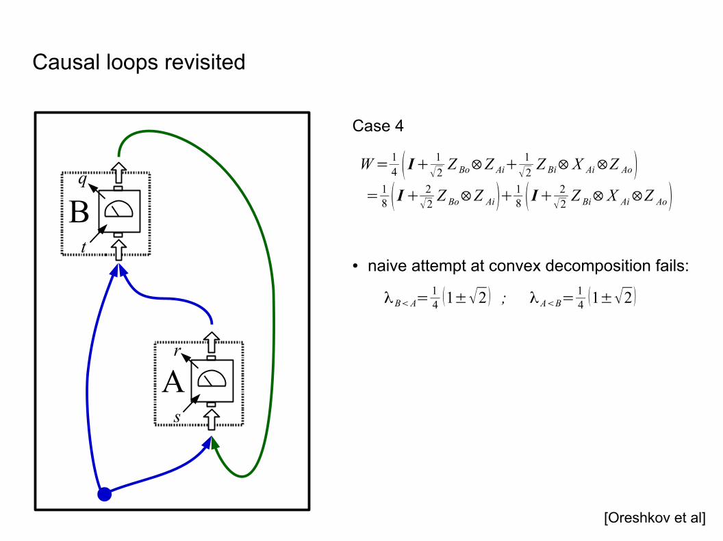
Case 4
● naive attempt at convex decomposition fails:
[Oreshkov et al]
W= 14 ( I+ 1
√2Z Bo⊗Z Ai+
1
√2Z Bi⊗X Ai⊗Z Ao )
= 18 ( I+ 2
√2Z Bo⊗Z Ai )+ 1
8 ( I+ 2√2
Z Bi⊗X Ai⊗Z Ao )
Causal loops revisited
λB<A=14(1±√2 ) ; λA<B=
14(1±√2 )
As
r
Bt
q
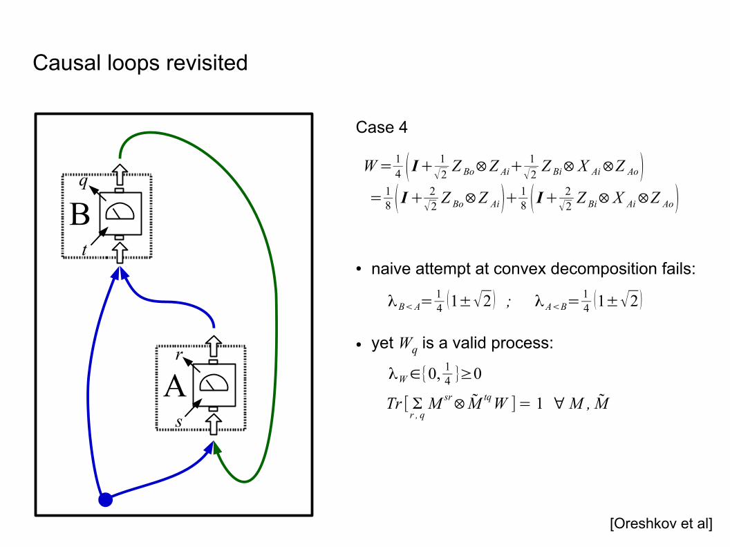
Case 4
● naive attempt at convex decomposition fails:
● yet Wq is a valid process:
[Oreshkov et al]
W= 14 ( I+ 1
√2Z Bo⊗Z Ai+
1
√2Z Bi⊗X Ai⊗Z Ao )
= 18 ( I+ 2
√2Z Bo⊗Z Ai )+ 1
8 ( I+ 2√2
Z Bi⊗X Ai⊗Z Ao )
Causal loops revisited
λB<A=14(1±√2 ) ; λA<B=
14(1±√2 )
As
r
Bt
q
Tr [ Σr , q
M sr⊗M tqW ]= 1 ∀M , M
λW∈{0, 14 }≥0
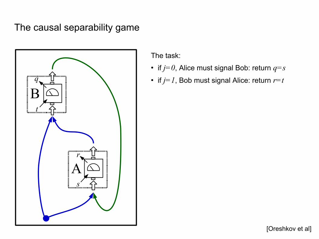
The causal separability game
As
r
Bt
q
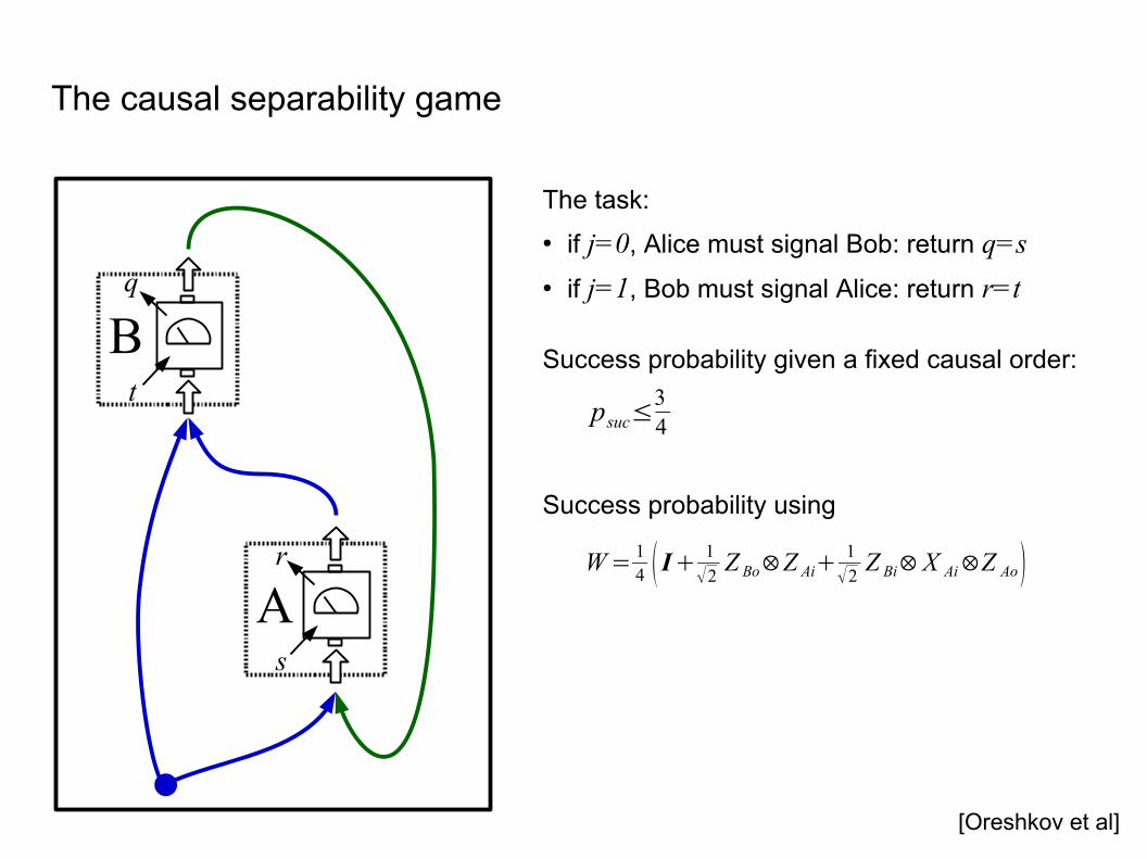
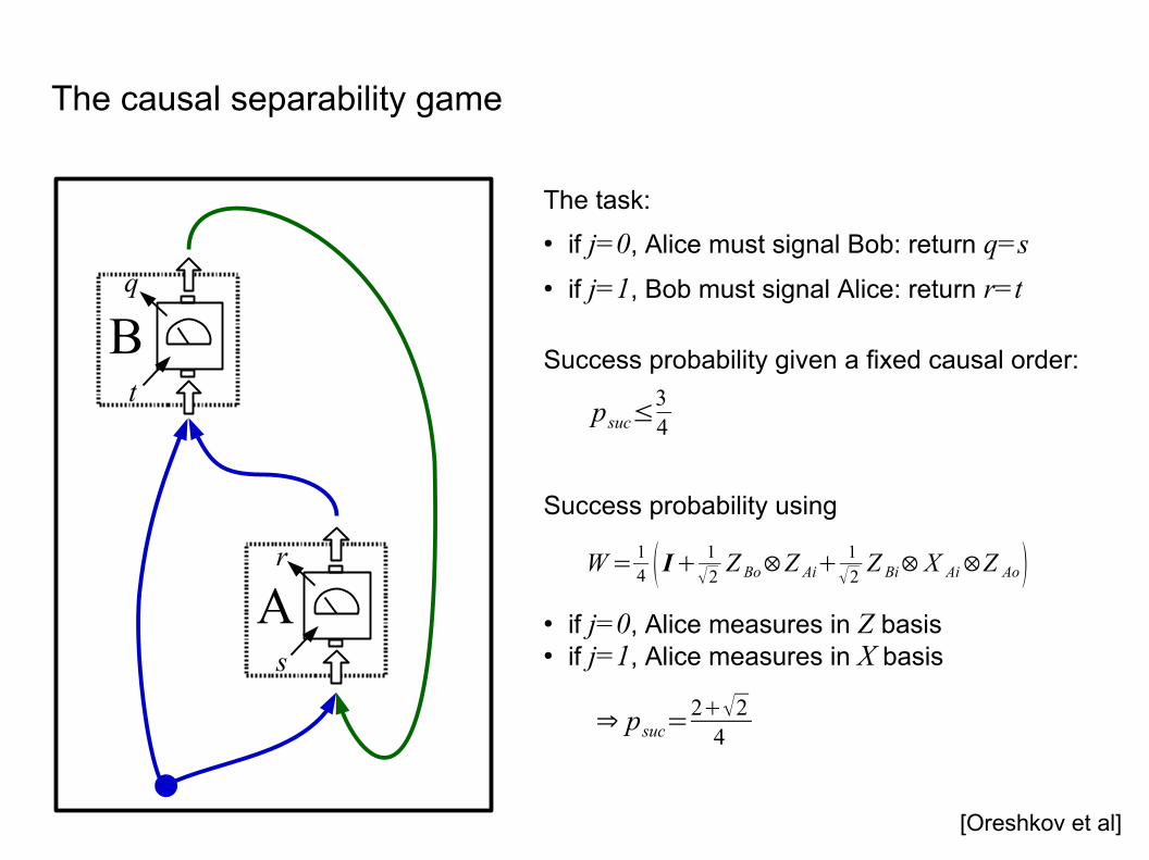
The task:
● if j=0, Alice must signal Bob: return q=s● if j=1, Bob must signal Alice: return r=t
[Oreshkov et al]
The causal separability game
As
r
Bt
q
The task:
● if j=0, Alice must signal Bob: return q=s● if j=1, Bob must signal Alice: return r=t
Success probability given a fixed causal order:
Success probability using
psuc≤34
[Oreshkov et al]
W= 14 ( I+ 1
√2Z Bo⊗Z Ai+
1
√2Z Bi⊗X Ai⊗Z Ao)
The causal separability game
As
r
Bt
q
The task:
● if j=0, Alice must signal Bob: return q=s● if j=1, Bob must signal Alice: return r=t
Success probability given a fixed causal order:
Success probability using
● if j=0, Alice measures in Z basis● if j=1, Alice measures in X basis
psuc≤34
[Oreshkov et al]
W= 14 ( I+ 1
√2Z Bo⊗Z Ai+
1
√2Z Bi⊗X Ai⊗Z Ao)
⇒ psuc=2+√2
4
Causal witnesses
As
r
Bt
q
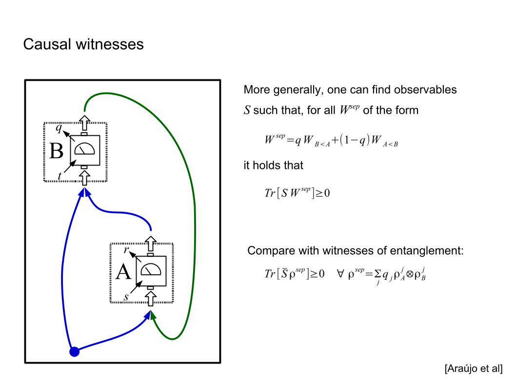
More generally, one can find observables
S such that, for all Wsep of the form
it holds that
[Araújo et al]
W sep=qW B<A+(1−q)W A<B
Tr [S W sep ]≥0
Compare with witnesses of entanglement:
Tr [ S ρsep ]≥0 ∀ ρsep=Σjq jρA
j⊗ρBj
Distinction: ● witnesses test separability, which is
a mathematical feature that isdefined within the framework ofquantum mechanics
● causal inequalities are device-independent, statistics-based tests
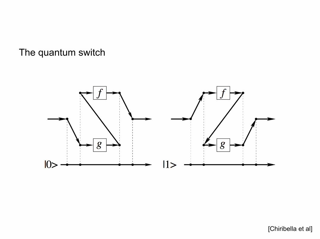
The quantum switch
[Chiribella et al]
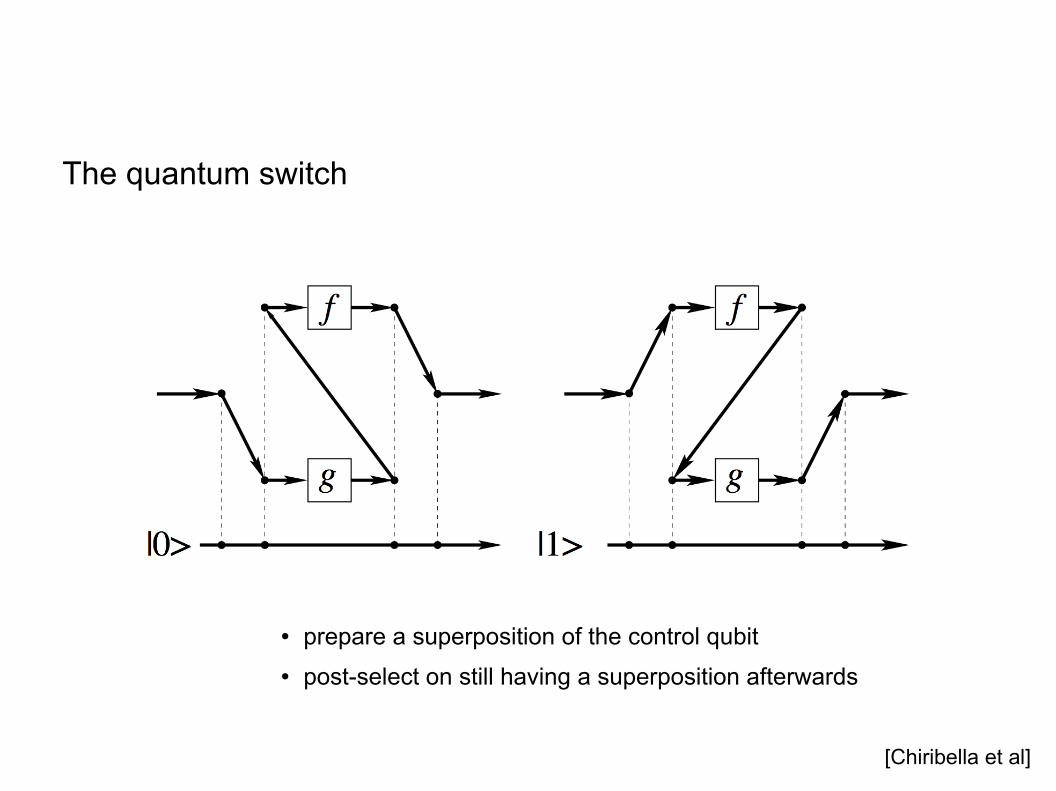
The quantum switch
[Chiribella et al]
● prepare a superposition of the control qubit
● post-select on still having a superposition afterwards
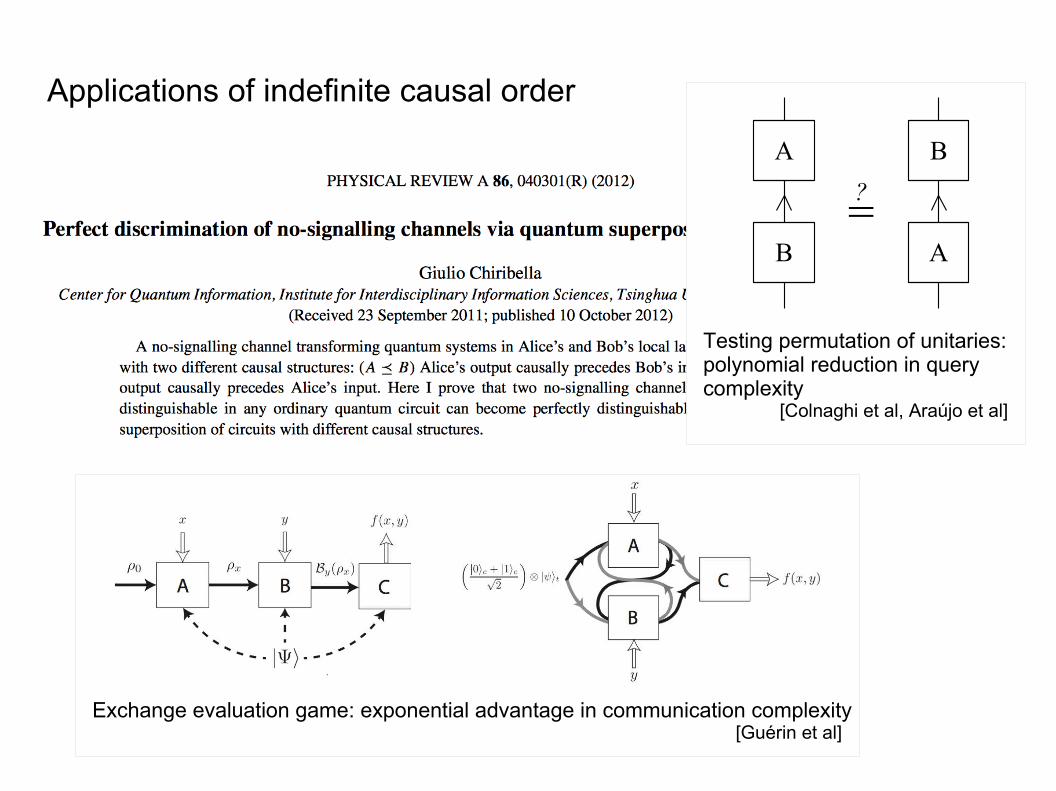
Applications of indefinite causal order
Exchange evaluation game: exponential advantage in communication complexity [Guérin et al]
Testing permutation of unitaries:polynomial reduction in querycomplexity
[Colnaghi et al, Araújo et al]
A
B
B
A
=?
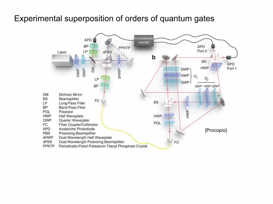
[Procopio]
Experimental superposition of orders of quantum gates
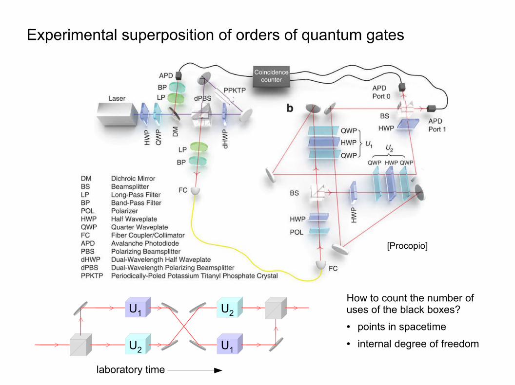
[Procopio]
Experimental superposition of orders of quantum gates
U1
U1
U2
U2
laboratory time
How to count the number ofuses of the black boxes?
● points in spacetime
● internal degree of freedom
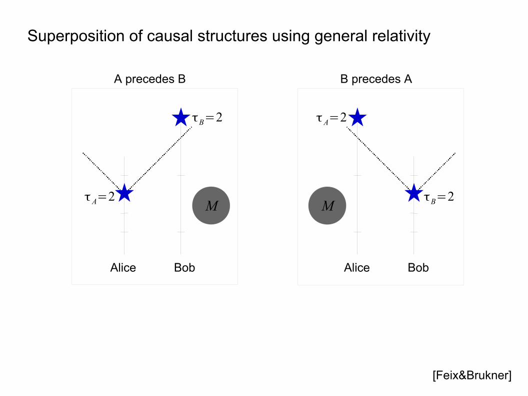
Superposition of causal structures using general relativity
[Feix&Brukner]
MτA=2
τB=2
A precedes B
Alice Bob
MτB=2
τA=2
B precedes A
Alice Bob
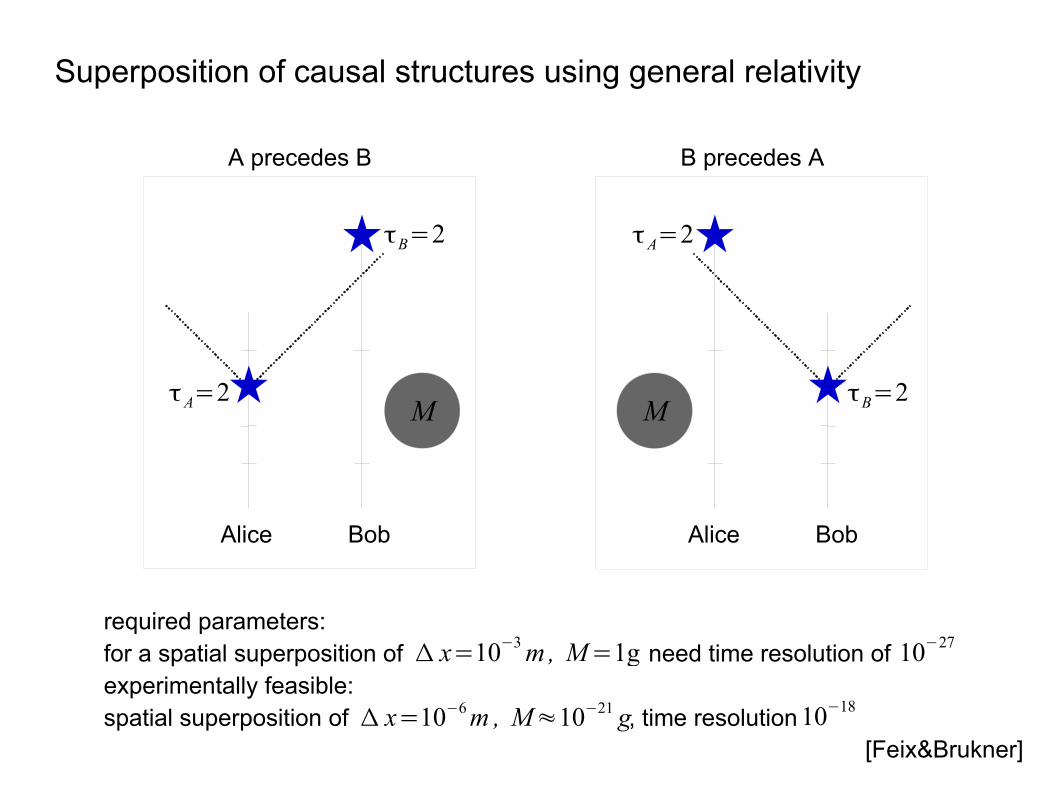
Superposition of causal structures using general relativity
[Feix&Brukner]
MτA=2
τB=2
A precedes B
Alice Bob
MτB=2
τA=2
B precedes A
Alice Bob
required parameters:for a spatial superposition of need time resolution ofexperimentally feasible:spatial superposition of , time resolution Δ x=10−6m , M≈10−21 g
Δ x=10−3 m, M=1g 10−27
10−18
Causal Structure in a Quantum World
Combinations of causal relations
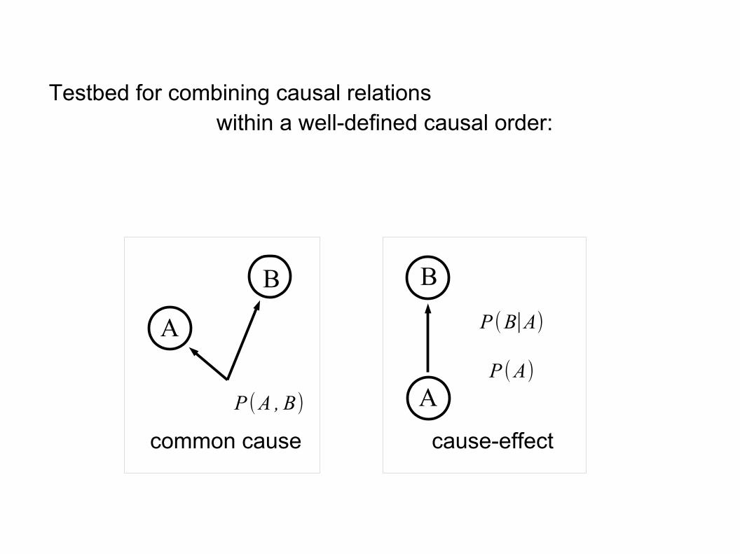
Testbed for combining causal relationswithin a well-defined causal order:
cause-effectcommon cause
A
B
A
B
P(A , B)
P(B∣A)
P (A)
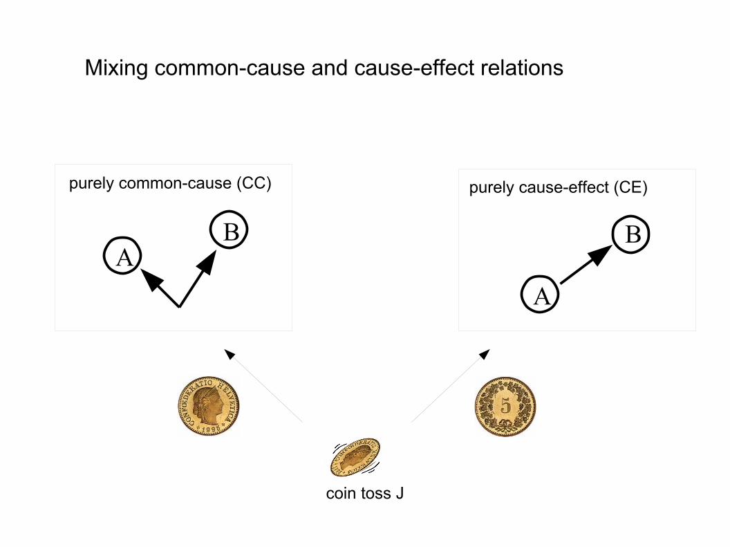
Mixing common-cause and cause-effect relations
coin toss J
purely common-cause (CC) purely cause-effect (CE)
A
BA
B
P(B|A,λ,heads)=P(B|λ)
purely common-cause
P(B|A,λ,tails)=P(B|A)
purely cause-effect
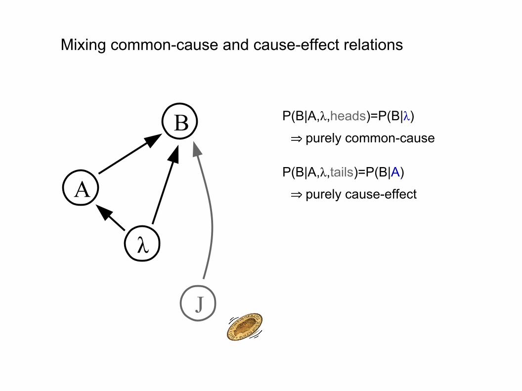
Mixing common-cause and cause-effect relations
A
B
J
λ
⇒
⇒
P(B|A,λ,heads)=P(B|λ)
purely common-cause
P(B|A,λ,tails)=P(B|A)
purely cause-effect
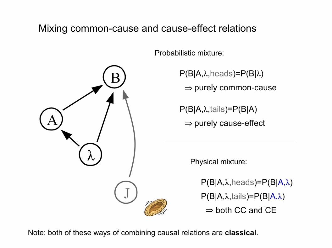
Mixing common-cause and cause-effect relations
A
B
λ
⇒
⇒
Probabilistic mixture:
Physical mixture:
P(B|A,λ,heads)=P(B|A,λ)
P(B|A,λ,tails)=P(B|A,λ)
both CC and CE⇒J
Note: both of these ways of combining causal relations are classical.
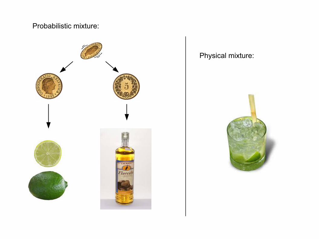
Probabilistic mixture:
Physical mixture:
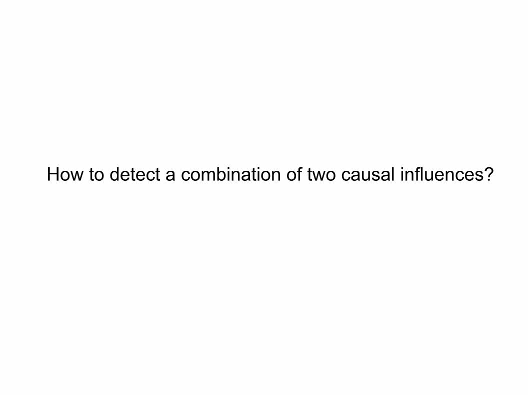
How to detect a combination of two causal influences?
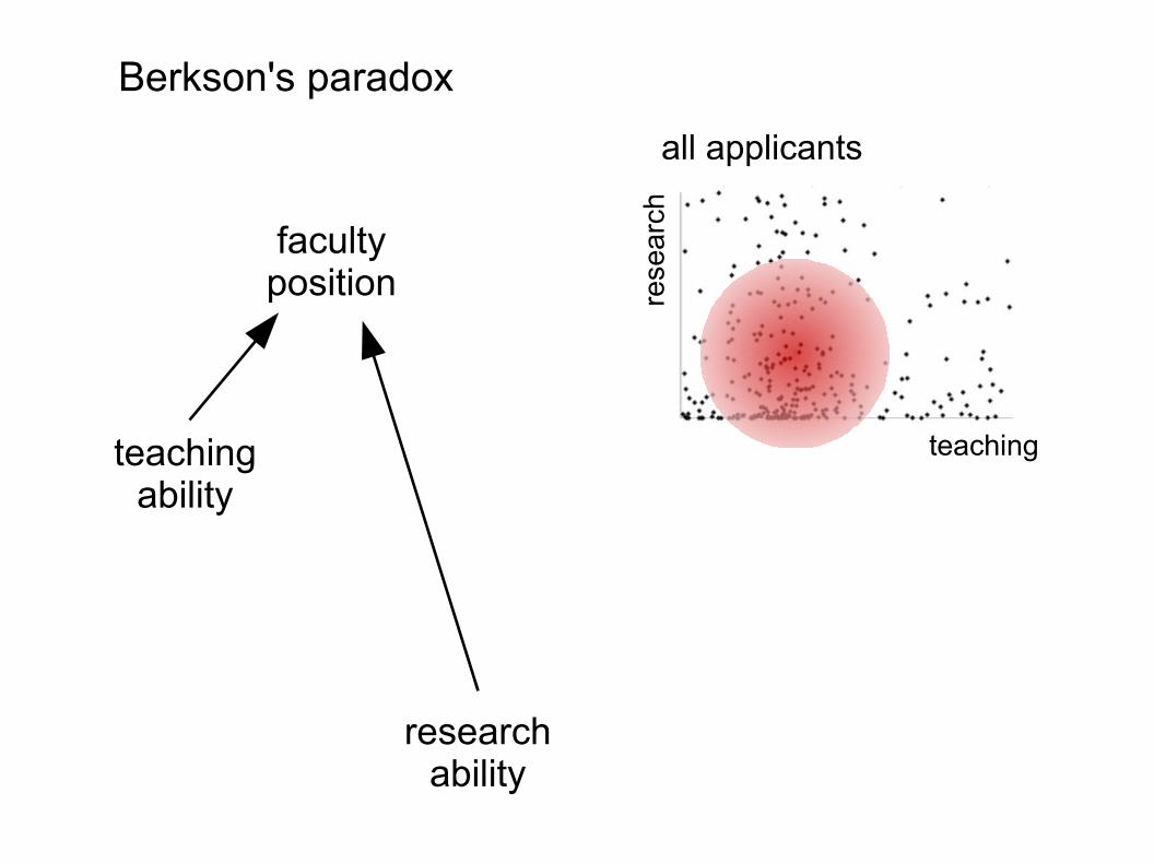
all applicants
teaching
rese
arch
teachingability
facultyposition
researchability
Berkson's paradox
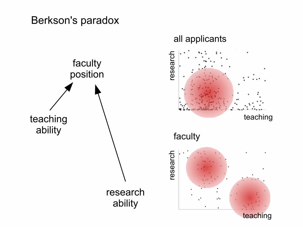
all applicants
faculty
teaching
teaching
rese
arch
teachingability
facultyposition
researchability
rese
arch
Berkson's paradox
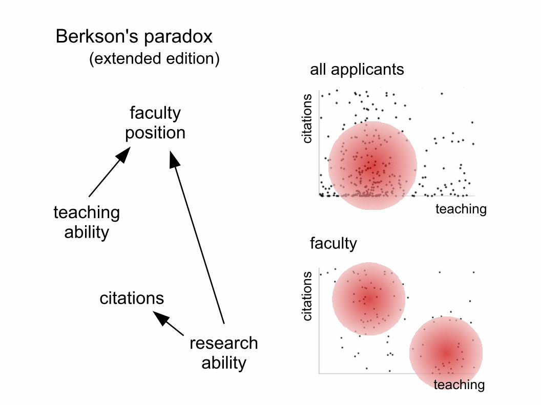
Berkson's paradox (extended edition)
all applicants
faculty
teaching
teaching
cita
tion
s
teachingability
facultyposition
researchability
citationsci
tatio
ns
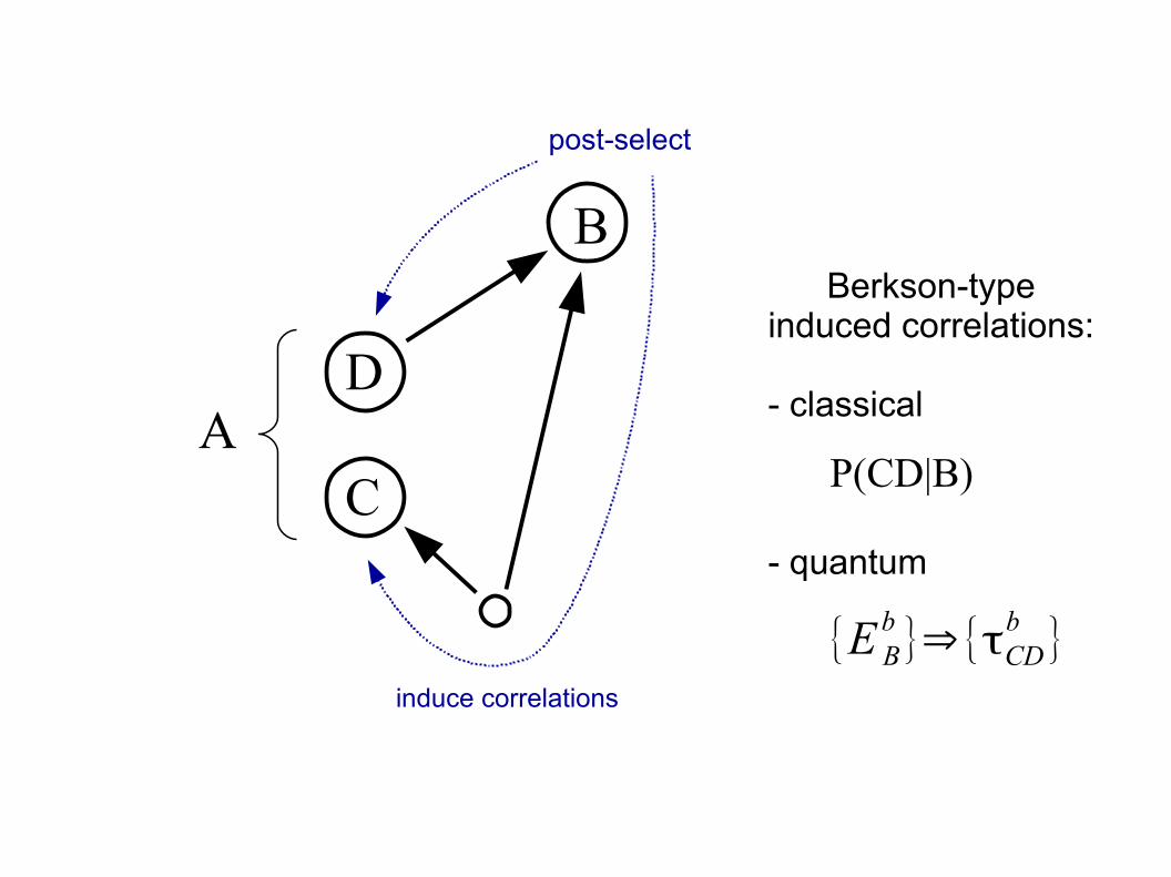
D
B
CA
P(CD|B)
Berkson-typeinduced correlations:
- classical
- quantum
post-select
induce correlations
{E Bb }⇒{τCD
b }
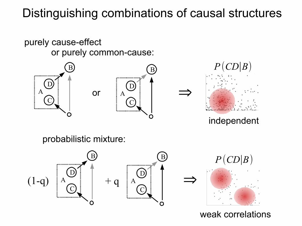
purely cause-effect or purely common-cause:
weak correlations
Distinguishing combinations of causal structures
C
B
DA
independent
P (CD∣B)
C
B
DA
P (CD∣B)
probabilistic mixture:
C
B
DA
C
B
DA
or
(1-q) + q ⇒
⇒
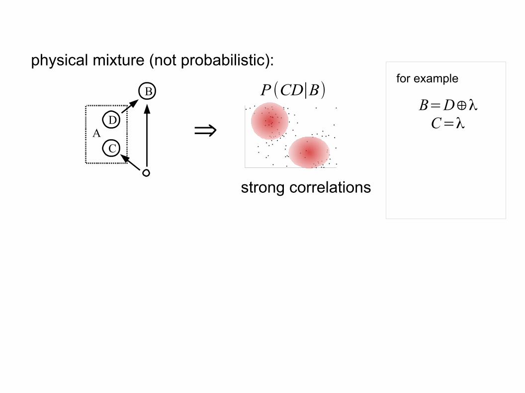
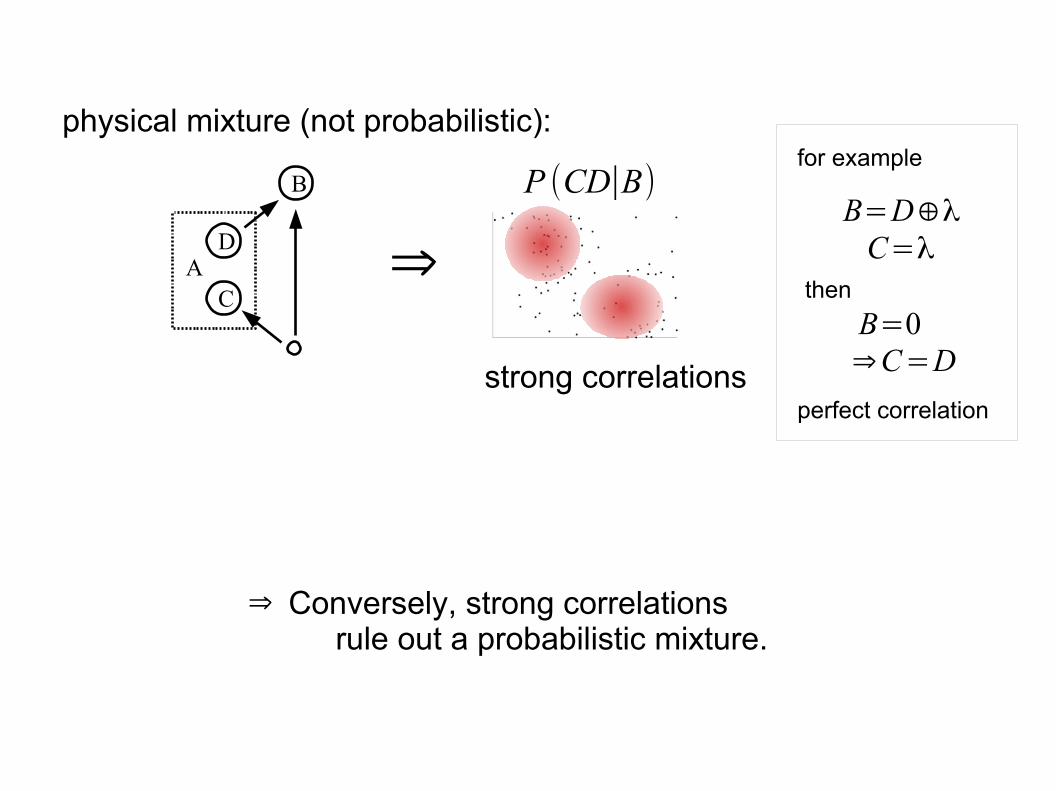
physical mixture (not probabilistic):
C
B
DA
strong correlations
P (CD∣B)
⇒B=D⊕λC=λ
for example
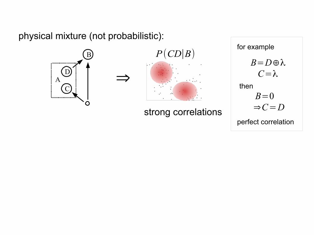
physical mixture (not probabilistic):
C
B
DA
strong correlations
P (CD∣B)
⇒B=D⊕λC=λ
for example
then
B=0⇒C=D
perfect correlation
physical mixture (not probabilistic):
C
B
DA
strong correlations
P (CD∣B)
⇒B=D⊕λC=λ
for example
then
B=0⇒C=D
perfect correlation
Conversely, strong correlations rule out a probabilistic mixture.
⇒

physical mixture (not probabilistic):
C
B
DA
strong correlations
P (CD∣B)
C
B
DA
τ(CD∣B)≠ΣiρC(i)⊗ρD
(i )
stronger-than-classicalcorrelations
⇒
intrinsically quantum combination:
⇒
for example
then
B=0⇒C=D
perfect correlation
B=D⊕λC=λ
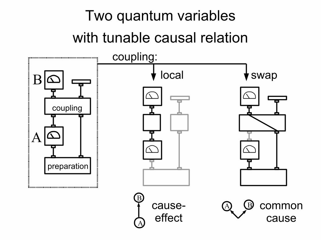
B
A
preparation
coupling
local swap
cause-effect
commoncause
coupling:
Two quantum variables
with tunable causal relation
A
BA B
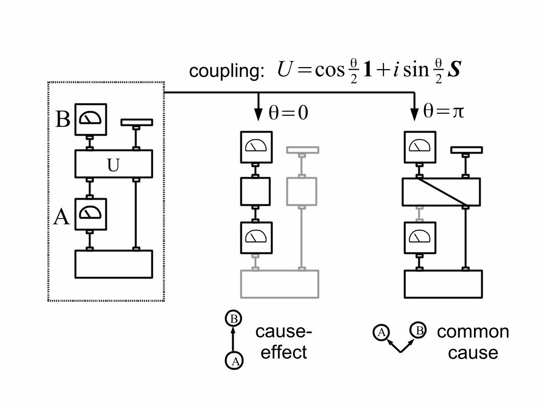
B
A
U
cause-effect
commoncause
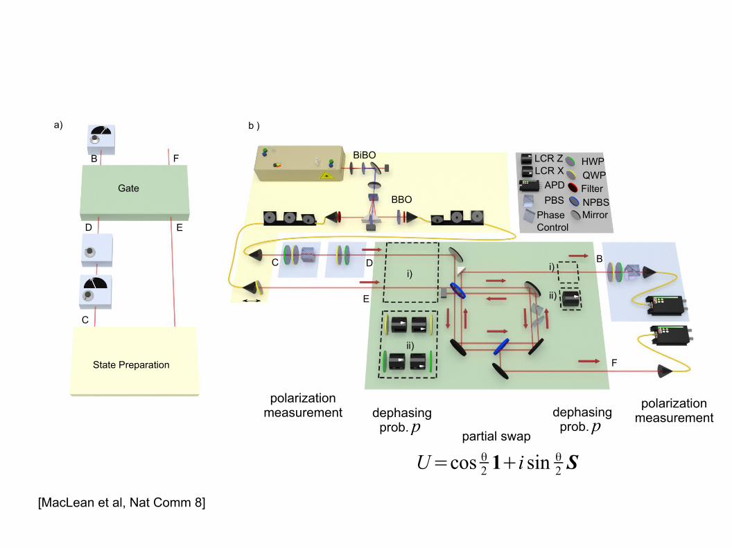
coupling: U=cos θ2 1+i sin θ2 S
θ=0 θ=π
A
BA B
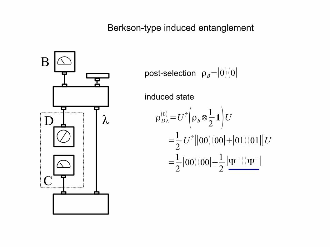
ρDλ(0)=U † (ρB⊗
121)U
=12
U † [∣00 ⟩ ⟨00∣+∣01 ⟩ ⟨01∣]U
=12∣00 ⟩ ⟨00∣+1
2∣Ψ− ⟩ ⟨Ψ−∣
ρB=∣0 ⟩ ⟨0∣
C
D
B
λ
Berkson-type induced entanglement
post-selection
induced state
ii)
ii)
a)
F
LCR Z
PBS
HWP
QWPFilterAPD
MirrorNPBS
Phase Control
BBO
BiBO
C BD
Gate
State Preparation
E
LCR X
C
B
D E
ii)
i)
b )
i)
ii)
F
F
partial swap
polarizationmeasurement
U=cos θ2 1+i sin θ2 S
dephasing prob. p
dephasing prob. p
polarizationmeasurement
[MacLean et al, Nat Comm 8]
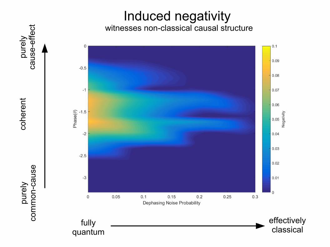
fully
quantum
effectivelyclassical
pure
lyco
mm
on-
caus
epu
rely
caus
e-e
ffec
tco
here
nt
Induced negativity witnesses non-classical causal structure

Take-home messages and open questions
Take-home messages and open questions
Causal models framework: mathematical and conceptual toolbox● classical: rigorous definition of causation, methods for inferring causal relations and
deriving predictions from this information● quantum: description of relations among quantum systems in terms of operators that can
(at least in part) be interpreted causally, distinction between causation and inference
Causal models provide a clear language and context for analysing many counter-intuitive phenomena in quantum mechanics, such as the apparent retrocausalityin delayed-choice experiments, propagation outside the lightcone in quantumfield theory, and the tangle of assumptions the lead to Bell inequalities.
The conjunction of all the principles that hold in classical causal models (Reichenbach,no fine-tuning etc) is at odds with the predictions of quantum mechanics. However, itis difficult to determine which of these principles are violated. More work is needed todevelop a convincing, consistent account of causality that allows one to give up any ofthese princples.
Take-home messages and open questions
Two proposals for how quantum mechanics might handle causal loops:● allow generic causal loops but give up linearity, which leads to
unusual information flow● preserve linearity but allow only a restricted class of causal loops
Non-classical causal relations● There are a few concrete examples of such scenarios, but a systematic
account of all the possibilities is still outstanding.● Some have been realized experimentally, but all experiments so far were
embedded in a background spacetime with well-defined causal order. Itwould be interesting to overcome this limitation.
● Non-classical causal structures are known to be resources for certaintasks. What other advantages can be extracted from these phenomenaand what fundamental insights does this entail?
References
Classical causal models:● A. Falcon, "Aristotle on Causality", The Stanford Encyclopedia of Philosophy (Spring 2015 Edition),
Edward N. Zalta (ed.), https://plato.stanford.edu/archives/spr2015/entries/aristotle-causality/.● David Hume, An enquiry concerning human understanding (1748), sect 7● Hans Reichenbach, The Direction of Time (University of California Press, 1956), sect. 19● David Tong, Quantum Field Theory (University of Cambridge Part III Mathematical Tripos)● Bertrand Russell, On the notion of cause, Proc Aristot Soc (1913) 13 (1): 1-26● Pearl, J. Causality: Models, Reasoning, and Inference (Cambridge Univ. Press, 2000).● P. Spirtes, C. Glymour, and R. Scheines, Causation, Prediction, and Search, (MIT Press, 2000).● S. W. Hawking, A. R. King, and P. J. McCarthy, J Math Phys 17, 174 (1976).● David B. Malament, J Math Phys 18, 1399 (1977)
Retrocausality and causal loops● Kim et al, „A Delayed Choice Quantum Eraser“, PhysRevLett 84,1 (2000), arXiv:quant-ph/9903047● Y. Aharonov, P.G. Bergmann and J. L. Lebowitz, „Time symmetry in the quantum process of
measurement“, PhysRevB 134, 1410 (1964).● L. Vaidman, „The two-state vector formalism“, arXiv:0706.1347● C. Ferrie and J. Combes, „How the result of a single coin toss can turn out to be 100 heads“, Phys.
Rev. Lett. 113, 120404 (2014)● W. J.van Stockum, Proc. R. Soc. Edinb. 57, 135 (1937); K. Gödel, RevModPhys 21, 447 (1949); F. J.
Tipler PhysRevD 9, 2203 (1974)● D. Deutsch, „Quantum mechanics near closed timelike lines“, PhysRevD 44, 3197(1991)● T.C. Ralph and C.R. Myers „Information flow of quantum states interacting with closed timelike
curves“, PhysRevA 82, 062330 (2010)● S. Aaronson and J. Watrous, „Closed Timelike Curves Make Quantum and Classical Computing
Equivalent“,Proc. R. Soc. A (2009) 465, 631 (2008), arXiv:0808.2669
References
Nonlocality● M. E. Peskin & D. V. Schroeder, An Introduction to Quantum Field Theory (Perseus Books, 1995), Ch. 2 ● Howard M. Wiseman and Eric G. Cavalcanti, "Causarum Investigatio and the Two Bell's Theorems of John Bell" in
"Quantum [Un]Speakables II: Half a Century of Bell's Theorem" (Springer), arXiv:1503.06413● C. J. Wood and R. W. Spekkens, „The lesson of causal discovery algorithms for quantum correlations: Causal
explanations of Bell-inequality violations require fine-tuning“, New J. Phys. 17, 033002 (2015), arXiv:1208.4119
Quantum Causal Models● Choi, M. D. Completely positive linear maps on complex matrices. Lin Alg Appl 10 , 285–290 (1975).● Jamiołkowski, A. Linear transformations which preserve trace and positive semidefiniteness of operators. Rep.
Math. Phys. 3 , 275–278 (1972).● G. Chiribella, G.M. D'Ariano & P. Perinotti, Theoretical framework for quantum networks. PRA 80, 022339 (2009) ● O. Oreshkov, F. Costa, C. Brukner, Quantum correlations with no causal order, Nat Comm 3, 1092 (2012)● Leifer, M. S. & Spekkens, R. W. Towards a formulation of quantum theory as a causally neutral theory of Bayesian
inference. Phys. Rev. A 88, 052130 (2013).● D. Horsman et al, Can a quantum state over time resemble a quantum state at a single time?, arxiv:1607.03637● K. Ried et al, Inferring causal structure: a quantum advantage, Nat Phys 11, 414-420 (2015), arXiv:1406.5036● M. Araújo et al, Witnessing causal nonseparability, New J. Phys. 17 (2015) 102001, arXiv:1506.03776
Computation with indefinite causal order● Chiribella, G., D'Ariano, G. M., Perinotti, P. & Valiron, B. Quantum computations without definite causal structure.
Phys. Rev. A 88, 022318 (2013), arXiv:0912.0195● Araújo, M., Costa, F. & Brukner, C. Computational advantage from quantum-controlled ordering of gates, Phys.
Rev. Lett. 113, 250402 (2014), arxiv:1401.8127● P. A. Guérin, A. Feix, M. Araújo and Č. Brukner, Exponential Communication Complexity Advantage from Quantum
Superposition of the Direction of Communication, Phys. Rev. Lett. 117, 100502 (2016).
Experiments on quantum causal structures● Procopio et al, „Experimental superposition of orders of quantum gates“, Nat Comm 6, 7913 (2015)● A. Feix, Č. Brukner, „Quantum superpositions of "common-cause" and "direct-cause" causal structures“,
arXiv:1606.09241 ● MacLean et al, „Quantum-coherent mixtures of causal relations“, Nat Comm 8, 15149 (2017), arXiv:1606.04523