Anti Bohr Quantum Theory and Causality - Semantic Scholar · principle of causality will expel any kind of mysticism from physics and enable a quantization of the . gravitational

Anti Bohr — Quantum Theory and Causality

Ilija Barukčić*

Internist. Horandstrasse, DE-26441 Jever, Germany. * Corresponding author. Tel.: 0700-56 56 56 56; email: [email protected] Manuscript submitted December 17, 2016; accepted February 3, 2017.

Abstract: The political attitude and the ideology of a very small elite of physicists (Niels Bohr, Werner

Heisenberg, Max Born and view other) played a major role in the construction of the Copenhagen

Interpretation of quantum mechanics in the 1920s. Lastly, the hegemonic standard acausal Copenhagen

Interpretation of quantum mechanics abandoned the principle of causality in quantum mechanics and

opened a very wide door to mysticism, logical fallacies and wishful thinking in physics and in science as

such. Historically, the Second International Congress for the Unity of Science (Copenhagen, June 21-26,

1936) tried to solve the problem of causality within physics but without a success. Thus far, 80 years after

the Second International Congress for the Unity of Science this publication will expel Bohr's and

Heisenberg's dogma of non-causality out of quantum mechanics and re-establish the unrestricted validity of

the principle of causality at quantum level and under conditions of relativity theory by mathematizing the

relationship between cause and effect in the form of the mathematical formula of the causal relationship k.

In contrast to Bohr, Heisenberg and other representatives of the Copenhagen interpretation quantum

mechanics, a realistic interpretation of quantum theory grounded on the unrestricted validity of the

principle of causality will expel any kind of mysticism from physics and enable a quantization of the

gravitational field too.

Key words: Causality, quantum theory, relativity theory, unified field theory.

1. Introduction

Since ancient times, the principle of causality was generally regarded as the most fundamental of all

principles, the demarcation line between science and non-science and our best candidate for a unique and

fundamental description of the physical world. But it may be useful to point out that the principle of

causality lost its scientific meaning at least since Heisenberg's publication of his uncertainty principle.

Heisenberg's himself considered his uncertainty principle to be the new cornerstone of science as such.

Heisenberg summarized his findings on the principle of causality in a general conclusion: "... so wird

durch die Quantenmechanik die Ungültigkeit des Kausalgesetzes definitiv festgestellt" [1] or in

broken English 'quantum mechanics has refuted the principle of causality definitely'. Apparently, even when

Bohr himself refers to the principle of causality, he supports Heisenberg's position. In fact, Bohr tried to

convince the assembly of scientists by explaining that the "so-called indeterminacy relations explicitly

bear out the limitation of causal analysis" [2] Let us conclude this short overview with Bohr's dogmatic

remark that "physics ... forces us to replace ... causality by ... complementarity" [3] By time, the

extraordinary predictive successes of quantum mechanics in power and precision, supported, at least at

first glance, more and more Heisenberg's uncertainty principle and the so-called Copenhagen interpretation

International Journal of Applied Physics and Mathematics

93 Volume 7, Number 2, April 2017

doi: 10.17706/ijapm.2017.7.2.93-111

2. Material and Methods

Definition 1. Bernoulli trials

A Bernoulli trial (or binomial trial) denotes a random experiment with exactly two possible outcomes,

either a concrete eigenvalue or not a concrete eigenvalue i. e. all but the concrete eigenvalue. The

mathematical formalization of the Bernoulli trial is denoted as the Bernoulli process. A random experiment

may consists of performing n Bernoulli trials, each with the probability p(jet) as associated with the

eigenvalue jet, i. e. it is t = +1, ..., +N.

Definition 2. Bernoulli observable

Let a Bernoulli random variable or a Bernoulli quantum mechanical observable be associated with a

quantum mechanical operator. Let the Bernoulli quantum mechanical observable be determined by the fact

that the same observable can take only two eigenvalues either +1 or +0 associated with some adequate

probabilities and eigenfunctions.

Property. In the language of set theory we obtain i. e. OCt ={+0, +1}.

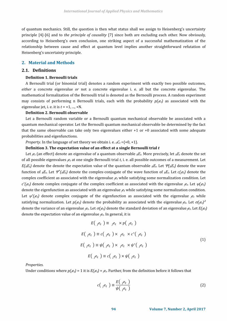
Definition 3. The expectation value of an effect at a single Bernoulli trial t

Let jet (an effect) denote an eigenvalue of a quantum observable REt. More precisely, let REt denote the set

of all possible eigenvalues jet at one single Bernoulli trial t, i. e. all possible outcomes of a measurement. Let

E(REt) denote the denote the expectation value of the quantum observable REt. Let (REt) denote the wave

function of REt. Let (REt) denote the complex-conjugate of the wave function of REt. Let c(jet) denote the

complex coefficient as associated with the eigenvalue jet while satisfying some normalization condition. Let

c*(jet) denote complex conjugate of the complex coefficient as associated with the eigenvalue jet. Let (jet)

denote the eigenfunction as associated with an eigenvalue jet while satisfying some normalization condition.

Let *(jet) denote complex conjugate of the eigenfunction as associated with the eigenvalue jet while

satisfying normalization. Let p(jet) denote the probability as associated with the eigenvalue jet. Let (jet)²

denote the variance of an eigenvalue jet. Let (jet) denote the standard deviation of an eigenvalue jet. Let E(jet)

denote the expectation value of an eigenvalue jet. In general, it is

𝐸( 𝑒𝑡𝑗 ) ≡ 𝑒𝑡𝑗 × 𝑝( 𝑒𝑡𝑗 )

𝐸( 𝑒𝑡𝑗 ) ≡ 𝑐( 𝑒𝑡𝑗 ) × 𝑒𝑡𝑗 × 𝑐∗( 𝑒𝑡𝑗 )

𝐸( 𝑒𝑡𝑗 ) ≡ 𝜓( 𝑒𝑡𝑗 ) × 𝑒𝑡𝑗 × 𝜓∗( 𝑒𝑡𝑗 )

𝐸( 𝑒𝑡𝑗 ) ≡ 𝑐( 𝑒𝑡𝑗 ) × 𝜓( 𝑒𝑡𝑗 )

(1)

Properties.

Under conditions where p(jet) = 1 it is E(jet) = jet. Further, from the definition before it follows that

𝑐( 𝑒𝑡𝑗 ) ≡

𝐸( 𝑒𝑡𝑗 )

𝜓( 𝑒𝑡𝑗 ) (2)

of quantum mechanics. Still, the question is then what status shall we assign to Heisenberg's uncertainty

principle [4]-[6] and to the principle of causality [7] since both are excluding each other. Now obviously,

according to Heisenberg's own conclusion, one striking aspect of a successful mathematization of the

relationship between cause and effect at quantum level implies another straightforward refutation of

Heisenberg's uncertainty principle.



2.1. Definitions

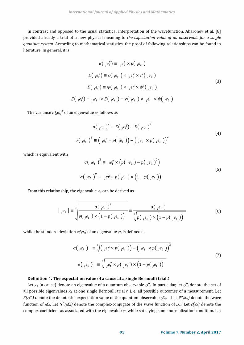
In contrast and opposed to the usual statistical interpretation of the wavefunction, Aharonov et al. [8]

provided already a trial of a new physical meaning to the expectation value of an observable for a single

quantum system. According to mathematical statistics, the proof of following relationships can be found in

literature. In general, it is

𝐸( 𝑒𝑡2

𝑗 ) ≡ 𝑒𝑡2

𝑗 × 𝑝( 𝑒𝑡𝑗 )

𝐸( 𝑒𝑡2

𝑗 ) ≡ 𝑐( 𝑒𝑡𝑗 ) × 𝑒𝑡2

𝑗 × 𝑐∗( 𝑒𝑡𝑗 )

𝐸( 𝑒𝑡2

𝑗 ) ≡ 𝜓( 𝑒𝑡𝑗 ) × 𝑒𝑡2

𝑗 × 𝜓∗( 𝑒𝑡𝑗 )

𝐸( 𝑒𝑡2

𝑗 ) ≡ 𝑒𝑡𝑗 × 𝐸( 𝑒𝑡𝑗 ) ≡ 𝑐( 𝑒𝑡𝑗 ) × 𝑒𝑡𝑗 × 𝜓( 𝑒𝑡𝑗 )

(3)

The variance (jet)² of an eigenvalue jet follows as

𝜎( 𝑒𝑡𝑗 )2≡ 𝐸( 𝑒𝑡

2𝑗 ) − 𝐸( 𝑒𝑡𝑗 )

2

𝜎( 𝑒𝑡𝑗 )2≡ ( 𝑒𝑡

2𝑗 × 𝑝( 𝑒𝑡𝑗 )) − ( 𝑒𝑡𝑗 × 𝑝( 𝑒𝑡𝑗 ))

2 (4)

which is equivalent with

𝜎( 𝑒𝑡𝑗 )2≡ 𝑒𝑡

2𝑗 × (𝑝( 𝑒𝑡𝑗 ) − 𝑝( 𝑒𝑡𝑗 )

2)

𝜎( 𝑒𝑡𝑗 )2≡ 𝑒𝑡

2𝑗 × 𝑝( 𝑒𝑡𝑗 ) × (1 − 𝑝( 𝑒𝑡𝑗 ))

(5)

From this relationship, the eigenvalue jet can be derived as

| 𝑒𝑡𝑗 | ≡ √𝜎( 𝑒𝑡𝑗 )

2

𝑝( 𝑒𝑡𝑗 ) × (1 − 𝑝( 𝑒𝑡𝑗 ))

2

≡𝜎( 𝑒𝑡𝑗 )

√𝑝( 𝑒𝑡𝑗 ) × (1 − 𝑝( 𝑒𝑡𝑗 ))2

(6)

while the standard deviation (jet) of an eigenvalue jet is defined as

𝜎( 𝑒𝑡𝑗 ) ≡ √( 𝑒𝑡

2𝑗 × 𝑝( 𝑒𝑡𝑗 )) − ( 𝑒𝑡𝑗 × 𝑝( 𝑒𝑡𝑗 ))

22

𝜎( 𝑒𝑡𝑗 ) ≡ √ 𝑒𝑡2

𝑗 × 𝑝( 𝑒𝑡𝑗 ) × (1 − 𝑝( 𝑒𝑡𝑗 ))2

(7)

Definition 4. The expectation value of a cause at a single Bernoulli trial t

Let ict (a cause) denote an eigenvalue of a quantum observable OCt. In particular, let OCt denote the set of

all possible eigenvalues ict at one single Bernoulli trial t, i. e. all possible outcomes of a measurement. Let

E(OCt) denote the denote the expectation value of the quantum observable OCt. Let (OCt) denote the wave

function of OCt. Let (OCt) denote the complex-conjugate of the wave function of OCt. Let c(ict) denote the

complex coefficient as associated with the eigenvalue ict while satisfying some normalization condition. Let



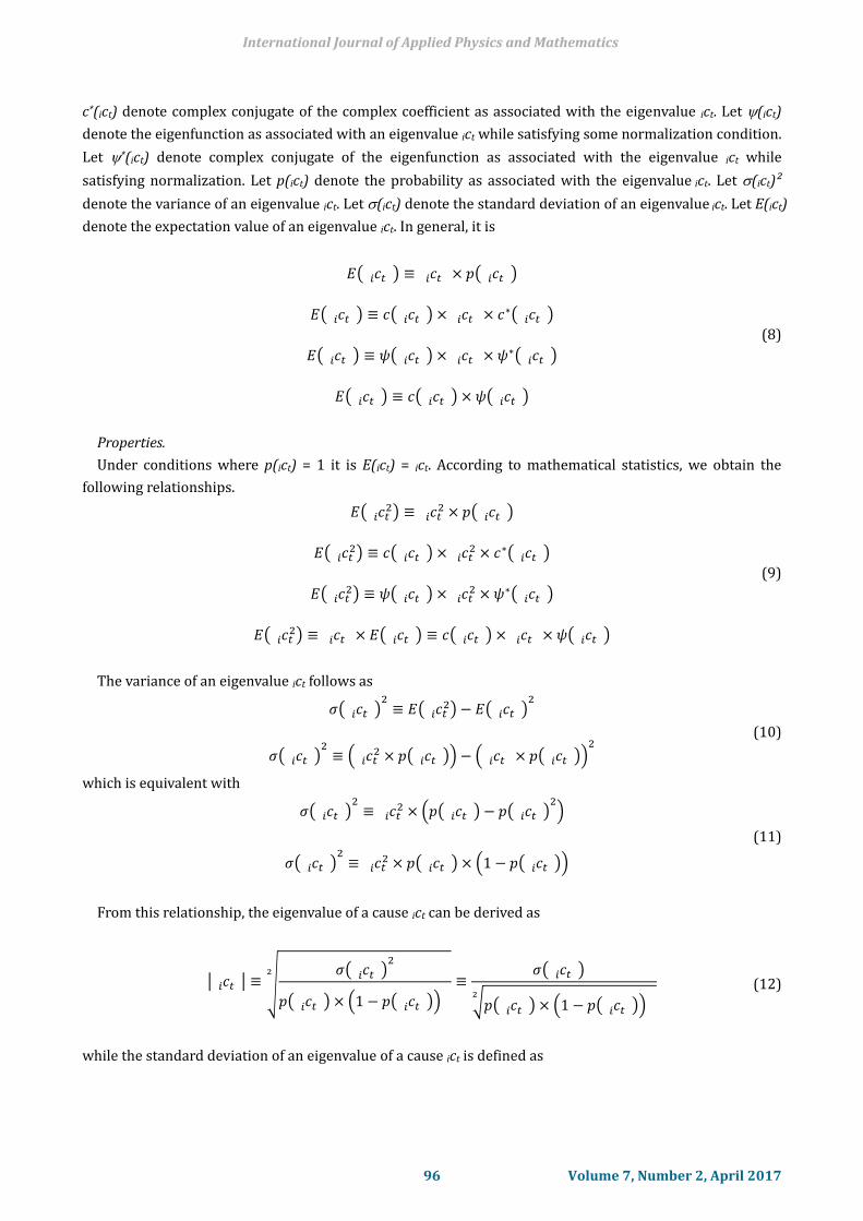
c*(ict) denote complex conjugate of the complex coefficient as associated with the eigenvalue ict. Let (ict)

denote the eigenfunction as associated with an eigenvalue ict while satisfying some normalization condition.

Let *(ict) denote complex conjugate of the eigenfunction as associated with the eigenvalue ict while

satisfying normalization. Let p(ict) denote the probability as associated with the eigenvalue ict. Let (ict)²

denote the variance of an eigenvalue ict. Let (ict) denote the standard deviation of an eigenvalue ict. Let E(ict)

denote the expectation value of an eigenvalue ict. In general, it is

𝐸( 𝑐𝑡𝑖 ) ≡ 𝑐𝑡𝑖 × 𝑝( 𝑐𝑡𝑖 )

𝐸( 𝑐𝑡𝑖 ) ≡ 𝑐( 𝑐𝑡𝑖 ) × 𝑐𝑡𝑖 × 𝑐∗( 𝑐𝑡𝑖 )

𝐸( 𝑐𝑡𝑖 ) ≡ 𝜓( 𝑐𝑡𝑖 ) × 𝑐𝑡𝑖 × 𝜓∗( 𝑐𝑡𝑖 )

𝐸( 𝑐𝑡𝑖 ) ≡ 𝑐( 𝑐𝑡𝑖 ) × 𝜓( 𝑐𝑡𝑖 )

(8)

Properties.

Under conditions where p(ict) = 1 it is E(ict) = ict. According to mathematical statistics, we obtain the

following relationships.

𝐸( 𝑐𝑡2

𝑖 ) ≡ 𝑐𝑡2

𝑖 × 𝑝( 𝑐𝑡𝑖 )

𝐸( 𝑐𝑡2

𝑖 ) ≡ 𝑐( 𝑐𝑡𝑖 ) × 𝑐𝑡2

𝑖 × 𝑐∗( 𝑐𝑡𝑖 )

𝐸( 𝑐𝑡2

𝑖 ) ≡ 𝜓( 𝑐𝑡𝑖 ) × 𝑐𝑡2

𝑖 × 𝜓∗( 𝑐𝑡𝑖 )

𝐸( 𝑐𝑡2

𝑖 ) ≡ 𝑐𝑡 ×𝑖 𝐸( 𝑐𝑡𝑖 ) ≡ 𝑐( 𝑐𝑡𝑖 ) × 𝑐𝑡𝑖 × 𝜓( 𝑐𝑡𝑖 )

(9)

The variance of an eigenvalue ict follows as

𝜎( 𝑐𝑡𝑖 )2≡ 𝐸( 𝑐𝑡

2𝑖 ) − 𝐸( 𝑐𝑡𝑖 )

2

𝜎( 𝑐𝑡𝑖 )2≡ ( 𝑐𝑡

2𝑖 × 𝑝( 𝑐𝑡𝑖 )) − ( 𝑐𝑡𝑖 × 𝑝( 𝑐𝑡𝑖 ))

2 (10)

which is equivalent with

𝜎( 𝑐𝑡𝑖 )2≡ 𝑐𝑡

2𝑖 × (𝑝( 𝑐𝑡𝑖 ) − 𝑝( 𝑐𝑡𝑖 )

2)

𝜎( 𝑐𝑡𝑖 )2≡ 𝑐𝑡

2𝑖 × 𝑝( 𝑐𝑡𝑖 ) × (1 − 𝑝( 𝑐𝑡𝑖 ))

(11)

From this relationship, the eigenvalue of a cause ict can be derived as

| 𝑐𝑡𝑖 | ≡ √𝜎( 𝑐𝑡𝑖 )

2

𝑝( 𝑐𝑡𝑖 ) × (1 − 𝑝( 𝑐𝑡𝑖 ))

2

≡𝜎( 𝑐𝑡𝑖 )

√𝑝( 𝑐𝑡𝑖 ) × (1 − 𝑝( 𝑐𝑡𝑖 ))2

(12)

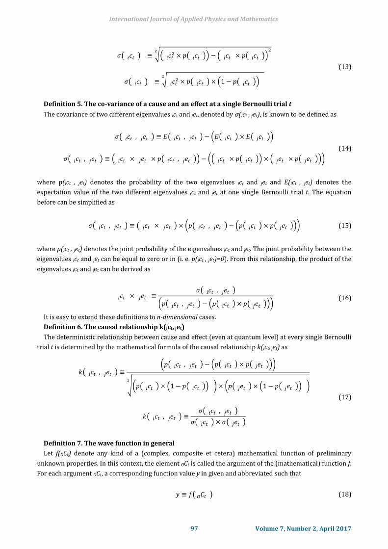
while the standard deviation of an eigenvalue of a cause ict is defined as



𝜎( 𝑐𝑡𝑖 ) ≡ √( 𝑐𝑡

2𝑖 × 𝑝( 𝑐𝑡𝑖 )) − ( 𝑐𝑡𝑖 × 𝑝( 𝑐𝑡𝑖 ))

22

𝜎( 𝑐𝑡𝑖 ) ≡ √ 𝑐𝑡2

𝑖 × 𝑝( 𝑐𝑡𝑖 ) × (1 − 𝑝( 𝑐𝑡𝑖 ))2

(13)

Definition 5. The co-variance of a cause and an effect at a single Bernoulli trial t

The covariance of two different eigenvalues ict and jet, denoted by (ict , jet), is known to be defined as

𝜎( 𝑐𝑡𝑖 , 𝑒𝑡𝑗 ) ≡ 𝐸( 𝑐𝑡𝑖 , 𝑒𝑡𝑗 ) − (𝐸( 𝑐𝑡𝑖 ) × 𝐸( 𝑒𝑡𝑗 ))

𝜎( 𝑐𝑡𝑖 , 𝑒𝑡𝑗 ) ≡ ( 𝑐𝑡𝑖 × 𝑒𝑡𝑗 × 𝑝( 𝑐𝑡𝑖 , 𝑒𝑡𝑗 )) − (( 𝑐𝑡𝑖 × 𝑝( 𝑐𝑡𝑖 )) × ( 𝑒𝑡𝑗 × 𝑝( 𝑒𝑡𝑗 )))

(14)

where p(ict , jet) denotes the probability of the two eigenvalues ict and jet and E(ict , jet) denotes the

expectation value of the two different eigenvalues ict and jet at one single Bernoulli trial t. The equation

before can be simplified as

𝜎( 𝑐𝑡𝑖 , 𝑒𝑡𝑗 ) ≡ ( 𝑐𝑡𝑖 × 𝑒𝑡𝑗 ) × (𝑝( 𝑐𝑡𝑖 , 𝑒𝑡𝑗 ) − (𝑝( 𝑐𝑡𝑖 ) × 𝑝( 𝑒𝑡𝑗 ))) (15)

where p(ict , jet) denotes the joint probability of the eigenvalues ict and jet. The joint probability between the

eigenvalues ict and jet can be equal to zero or in (i. e. p(ict , jet)=0). From this relationship, the product of the

eigenvalues ict and jet can be derived as

𝑐𝑡𝑖 × 𝑒𝑡𝑗 ≡

𝜎( 𝑐𝑡𝑖 , 𝑒𝑡𝑗 )

(𝑝( 𝑐𝑡𝑖 , 𝑒𝑡𝑗 ) − (𝑝( 𝑐𝑡𝑖 ) × 𝑝( 𝑒𝑡𝑗 ))) (16)

It is easy to extend these definitions to n-dimensional cases.

Definition 6. The causal relationship k(ict, jet)

The deterministic relationship between cause and effect (even at quantum level) at every single Bernoulli

trial t is determined by the mathematical formula of the causal relationship k(ict, jet) as

𝑘( 𝑐𝑡𝑖 , 𝑒𝑡𝑗 ) ≡(𝑝( 𝑐𝑡𝑖 , 𝑒𝑡𝑗 ) − (𝑝( 𝑐𝑡𝑖 ) × 𝑝( 𝑒𝑡𝑗 )))

√(𝑝( 𝑐𝑡𝑖 ) × (1 − 𝑝( 𝑐𝑡𝑖 )) ) × (𝑝( 𝑒𝑡𝑗 ) × (1 − 𝑝( 𝑒𝑡𝑗 )) )2

𝑘( 𝑐𝑡𝑖 , 𝑒𝑡𝑗 ) ≡𝜎( 𝑐𝑡𝑖 , 𝑒𝑡𝑗 )

𝜎( 𝑐𝑡𝑖 ) × 𝜎( 𝑒𝑡𝑗 )

(17)

Definition 7. The wave function in general

Let f(OCt) denote any kind of a (complex, composite et cetera) mathematical function of preliminary

unknown properties. In this context, the element OCt is called the argument of the (mathematical) function f.

For each argument OCt, a corresponding function value y in given and abbreviated such that

𝑦 ≡ 𝑓( 𝐶𝑡𝑂 ) (18)



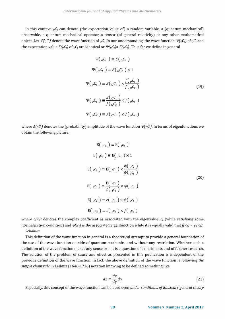
In this context, OCt can denote (the expectation value of) a random variable, a (quantum mechanical)

observable, a quantum mechanical operator, a tensor (of general relativity) or any other mathematical

object. Let (OCt) denote the wave function of OCt. In our understanding, the wave function (OCt) of OCt and

the expectation value E(OCt) of OCt are identical or (OCt)= E(OCt). Thus far we define in general

Ψ( 𝐶𝑡𝑂 ) ≡ 𝐸( 𝐶𝑡𝑂 )

Ψ( 𝐶𝑡𝑂 ) ≡ 𝐸( 𝐶𝑡𝑂 ) × 1

Ψ( 𝐶𝑡𝑂 ) ≡ 𝐸( 𝐶𝑡𝑂 ) ×𝑓( 𝐶𝑡𝑂 )

𝑓( 𝐶𝑡𝑂 )

Ψ( 𝐶𝑡𝑂 ) ≡𝐸( 𝐶𝑡𝑂 )

𝑓( 𝐶𝑡𝑂 )× 𝑓( 𝐶𝑡𝑂 )

Ψ( 𝐶𝑡𝑂 ) ≡ 𝐴( 𝐶𝑡𝑂 ) × 𝑓( 𝐶𝑡𝑂 )

(19)

where A(OCt) denotes the (probability) amplitude of the wave function (OCt). In terms of eigenfunctions we

obtain the following picture.

E( 𝑐𝑡𝑖 ) ≡ E( 𝑐𝑡𝑖 )

E( 𝑐𝑡𝑖 ) ≡ E( 𝑐𝑡𝑖 ) × 1

E( 𝑐𝑡𝑖 ) ≡ E( 𝑐𝑡𝑖 ) ×𝜓( 𝑐𝑡𝑖 )

𝜓( 𝑐𝑡𝑖 )

E( 𝑐𝑡𝑖 ) ≡E( 𝑐𝑡𝑖 )

𝜓( 𝑐𝑡𝑖 )× 𝜓( 𝑐𝑡𝑖 )

E( 𝑐𝑡𝑖 ) ≡ 𝑐( 𝑐𝑡𝑖 ) × 𝜓( 𝑐𝑡𝑖 )

E( 𝑐𝑡𝑖 ) ≡ 𝑐( 𝑐𝑡𝑖 ) × 𝑓( 𝑐𝑡𝑖 )

(20)

where c(ict) denotes the complex coefficient as associated with the eigenvalue ict (while satisfying some

normalization condition) and (ict) is the associated eigenfunction while it is equally valid that f(ict) =(ict).

Scholium.

This definition of the wave function in general is a theoretical attempt to provide a general foundation of

the use of the wave function outside of quantum mechanics and without any restriction. Whether such a

definition of the wave function makes any sense or not is a question of experiments and of further research.

The solution of the problem of cause and effect as presented in this publication is independent of the

previous definition of the wave function. In fact, the above definition of the wave function is following the

simple chain rule in Leibniz (1646-1716) notation knowing to be defined something like

𝑑𝑧 ≡

𝑑𝑧

𝑑𝑦𝑑𝑦 (21)

Especially, this concept of the wave function can be used even under conditions of Einstein’s general theory



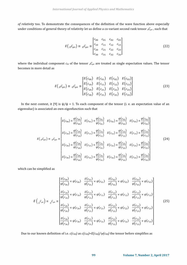
of relativity too. To demonstrate the consequences of the definition of the wave function above especially

under conditions of general theory of relativity let us define a co-variant second rank tensor oCµv , such that

𝐸( 𝐶𝜇𝜈𝑂 ) ≡ 𝐶𝜇𝜈𝑂 ≡

[ 𝑐00 𝑐01 𝑐02 𝑐03

𝑐10 𝑐11 𝑐12 𝑐13

𝑐20 𝑐21 𝑐22 𝑐23

𝑐30 𝑐31 𝑐32 𝑐33]

(22)

where the individual component cik of the tensor oCµv are treated as single expectation values. The tensor

becomes in more detail as


[ 𝐸(𝑐00) 𝐸(𝑐01) 𝐸(𝑐02) 𝐸(𝑐03)

𝐸(𝑐10) 𝐸(𝑐11) 𝐸(𝑐12) 𝐸(𝑐13)

𝐸(𝑐20) 𝐸(𝑐21) 𝐸(𝑐22) 𝐸(𝑐23)

𝐸(𝑐30) 𝐸(𝑐31) 𝐸(𝑐32) 𝐸(𝑐33)]

(23)

In the next context, it [9] is ψ/ψ = 1. To each component of the tensor (i. e. an expectation value of an

eigenvalue) is associated an own eigenfunction such that


[ 𝐸(𝑐00) ×

𝜓(𝑐00)

𝜓(𝑐00)𝐸(𝑐01) ×

𝜓(𝑐01)

𝜓(𝑐01)𝐸(𝑐02) ×

𝜓(𝑐02)

𝜓(𝑐02)𝐸(𝑐03) ×

𝜓(𝑐03)

𝜓(𝑐03)

𝐸(𝑐10) ×𝜓(𝑐10)

𝜓(𝑐10)𝐸(𝑐11) ×

𝜓(𝑐11)

𝜓(𝑐11)𝐸(𝑐12) ×

𝜓(𝑐12)

𝜓(𝑐12)𝐸(𝑐13) ×

𝜓(𝑐13)

𝜓(𝑐13)

𝐸(𝑐20) ×𝜓(𝑐20)

𝜓(𝑐20)𝐸(𝑐21) ×

𝜓(𝑐21)

𝜓(𝑐21)𝐸(𝑐22) ×

𝜓(𝑐22)

𝜓(𝑐22)𝐸(𝑐23) ×

𝜓(𝑐23)

𝜓(𝑐23)

𝐸(𝑐30) ×𝜓(𝑐30)

𝜓(𝑐30)𝐸(𝑐31) ×

𝜓(𝑐31)

𝜓(𝑐31)𝐸(𝑐32) ×

𝜓(𝑐32)

𝜓(𝑐32)𝐸(𝑐33) ×

𝜓(𝑐33)

𝜓(𝑐33)]

(24)

which can be simplified as

𝐸 ( 𝐶𝜇𝜈𝑂) ≡ 𝐶𝜇𝜈𝑂

≡

[ 𝐸(𝑐00)

𝜓(𝑐00)× 𝜓(𝑐00)

𝐸(𝑐01)

𝜓(𝑐01)× 𝜓(𝑐01)

𝐸(𝑐02)

𝜓(𝑐02)× 𝜓(𝑐02)

𝐸(𝑐03)

𝜓(𝑐03)× 𝜓(𝑐03)

𝐸(𝑐10)

𝜓(𝑐10)× 𝜓(𝑐10)

𝐸(𝑐11)

𝜓(𝑐11)× 𝜓(𝑐11)

𝐸(𝑐12)

𝜓(𝑐12)× 𝜓(𝑐12)

𝐸(𝑐13)

𝜓(𝑐13)× 𝜓(𝑐13)

𝐸(𝑐20)

𝜓(𝑐20)× 𝜓(𝑐20)

𝐸(𝑐21)

𝜓(𝑐21)× 𝜓(𝑐21)

𝐸(𝑐22)

𝜓(𝑐22)× 𝜓(𝑐22)

𝐸(𝑐23)

𝜓(𝑐23)× 𝜓(𝑐23)

𝐸(𝑐30)

𝜓(𝑐30)× 𝜓(𝑐30)

𝐸(𝑐31)

𝜓(𝑐31)× 𝜓(𝑐31)

𝐸(𝑐32)

𝜓(𝑐32)× 𝜓(𝑐32)

𝐸(𝑐33)

𝜓(𝑐33)× 𝜓(𝑐33)

]

(25)

Due to our known definition of i.e. c(c00) as c(c00)=E(c00)/(c00) the tensor before simplifies as



𝛹( 𝐶𝜇𝜈𝑂 ) ≡ 𝐸( 𝐶𝜇𝜈𝑂 ) ≡ 𝐶𝜇𝜈𝑂 ≡

[ 𝑐(𝑐00) × 𝜓(𝑐00) 𝑐(𝑐01) × 𝜓(𝑐01) 𝑐(𝑐02) × 𝜓(𝑐02) 𝑐(𝑐03) × 𝜓(𝑐03)

𝑐(𝑐10) × 𝜓(𝑐10) 𝑐(𝑐11) × 𝜓(𝑐11) 𝑐(𝑐12) × 𝜓(𝑐12) 𝑐(𝑐13) × 𝜓(𝑐13)

𝑐(𝑐20) × 𝜓(𝑐20) 𝑐(𝑐21) × 𝜓(𝑐21) 𝑐(𝑐22) × 𝜓(𝑐22) 𝑐(𝑐23) × 𝜓(𝑐23)

𝑐(𝑐30) × 𝜓(𝑐30) 𝑐(𝑐31) × 𝜓(𝑐31) 𝑐(𝑐32) × 𝜓(𝑐32) 𝑐(𝑐33) × 𝜓(𝑐33)]

(26)

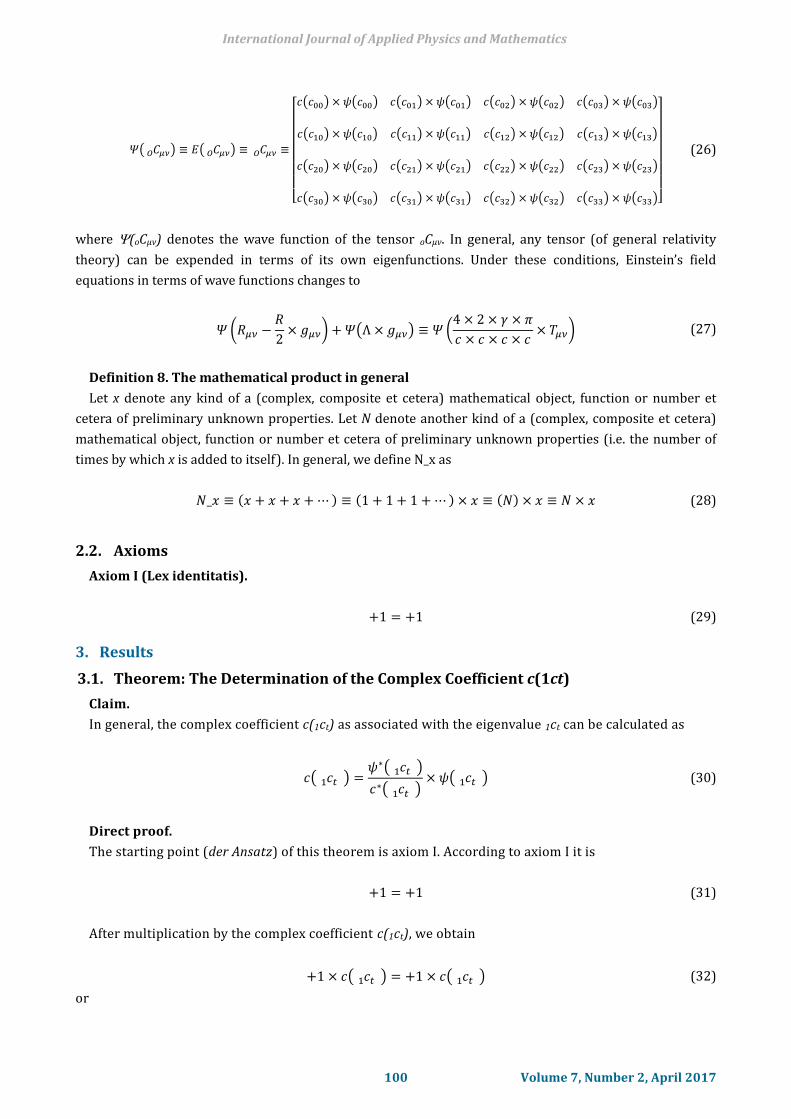
where (oCµv) denotes the wave function of the tensor oCµv. In general, any tensor (of general relativity

theory) can be expended in terms of its own eigenfunctions. Under these conditions, Einstein’s field

equations in terms of wave functions changes to

𝛹 (𝑅𝜇𝜈 −

𝑅

2× 𝑔𝜇𝜈) + 𝛹(Λ × 𝑔𝜇𝜈) ≡ 𝛹 (

4 × 2 × 𝛾 × 𝜋

𝑐 × 𝑐 × 𝑐 × 𝑐× 𝑇𝜇𝜈) (27)

Definition 8. The mathematical product in general

Let x denote any kind of a (complex, composite et cetera) mathematical object, function or number et

cetera of preliminary unknown properties. Let N denote another kind of a (complex, composite et cetera)

mathematical object, function or number et cetera of preliminary unknown properties (i.e. the number of

times by which x is added to itself). In general, we define N_x as

𝑁_𝑥 ≡ (𝑥 + 𝑥 + 𝑥 +⋯) ≡ (1 + 1 + 1 +⋯) × 𝑥 ≡ (𝑁) × 𝑥 ≡ 𝑁 × 𝑥 (28)

Axiom I (Lex identitatis).

+1 = +1 (29)

3. Results

Claim.

In general, the complex coefficient c(1ct) as associated with the eigenvalue 1ct can be calculated as

𝑐( 𝑐𝑡1 ) =

𝜓∗( 𝑐𝑡1 )

𝑐∗( 𝑐𝑡1 )× 𝜓( 𝑐𝑡1 ) (30)

Direct proof.

The starting point (der Ansatz) of this theorem is axiom I. According to axiom I it is

+1 = +1 (31)

After multiplication by the complex coefficient c(1ct), we obtain

+1 × 𝑐( 𝑐𝑡1 ) = +1 × 𝑐( 𝑐𝑡1 ) (32)

or



2.2. Axioms

3.1. Theorem: The Determination of the Complex Coefficient c(1ct)

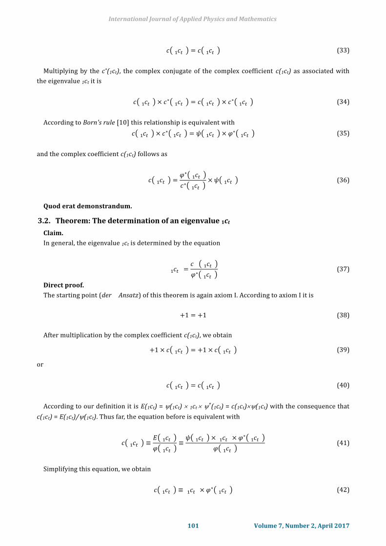
𝑐( 𝑐𝑡1 ) = 𝑐( 𝑐𝑡1 ) (33)

Multiplying by the c*(1ct), the complex conjugate of the complex coefficient c(1ct) as associated with

the eigenvalue 1ct it is

𝑐( 𝑐𝑡1 ) × 𝑐∗( 𝑐𝑡1 ) = 𝑐( 𝑐𝑡1 ) × 𝑐∗( 𝑐𝑡1 ) (34)

According to Born's rule [10] this relationship is equivalent with

𝑐( 𝑐𝑡1 ) × 𝑐∗( 𝑐𝑡1 ) = 𝜓( 𝑐𝑡1 ) × 𝜑∗( 𝑐𝑡1 ) (35)

and the complex coefficient c(1ct) follows as

𝑐( 𝑐𝑡1 ) =

𝜑∗( 𝑐𝑡1 )

𝑐∗( 𝑐𝑡1 )× 𝜓( 𝑐𝑡1 ) (36)

Quod erat demonstrandum.

Claim.

In general, the eigenvalue 1ct is determined by the equation

𝑐𝑡1 =

𝑐 ( 𝑐𝑡1 )

𝜑∗( 𝑐𝑡1 ) (37)

Direct proof.

The starting point (der Ansatz) of this theorem is again axiom I. According to axiom I it is

+1 = +1 (38)


+1 × 𝑐( 𝑐𝑡1 ) = +1 × 𝑐( 𝑐𝑡1 ) (39)

or

𝑐( 𝑐𝑡1 ) = 𝑐( 𝑐𝑡1 ) (40)

According to our definition it is E(1ct) = (1ct) 1ct (1ct) = c(1ct)(1ct) with the consequence that

c(1ct) = E(1ct)/(1ct). Thus far, the equation before is equivalent with

𝑐( 𝑐𝑡1 ) ≡

𝐸( 𝑐𝑡1 )

𝜑( 𝑐𝑡1 )≡𝜓( 𝑐𝑡1 ) × 𝑐𝑡1 × 𝜑∗( 𝑐𝑡1 )

𝜑( 𝑐𝑡1 ) (41)

Simplifying this equation, we obtain

𝑐( 𝑐𝑡1 ) ≡ 𝑐𝑡1 × 𝜑∗( 𝑐𝑡1 ) (42)



3.2. Theorem: The determination of an eigenvalue 1ct

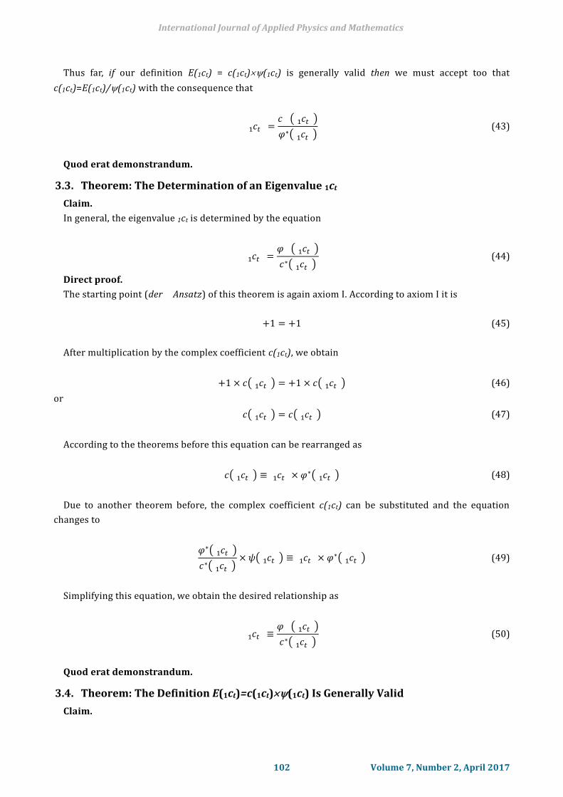
Thus far, if our definition E(1ct) = c(1ct)(1ct) is generally valid then we must accept too that

c(1ct)=E(1ct)/(1ct) with the consequence that

𝑐𝑡1 =

𝑐 ( 𝑐𝑡1 )

𝜑∗( 𝑐𝑡1 ) (43)


Claim.

In general, the eigenvalue 1ct is determined by the equation

𝑐𝑡1 =

𝜑 ( 𝑐𝑡1 )

𝑐∗( 𝑐𝑡1 ) (44)

Direct proof.


+1 = +1 (45)


+1 × 𝑐( 𝑐𝑡1 ) = +1 × 𝑐( 𝑐𝑡1 ) (46)

or

𝑐( 𝑐𝑡1 ) = 𝑐( 𝑐𝑡1 ) (47)

According to the theorems before this equation can be rearranged as

𝑐( 𝑐𝑡1 ) ≡ 𝑐𝑡1 × 𝜑∗( 𝑐𝑡1 ) (48)

Due to another theorem before, the complex coefficient c(1ct) can be substituted and the equation

changes to

𝜑∗( 𝑐𝑡1 )

𝑐∗( 𝑐𝑡1 )× 𝜓( 𝑐𝑡1 ) ≡ 𝑐𝑡1 × 𝜑∗( 𝑐𝑡1 ) (49)

Simplifying this equation, we obtain the desired relationship as

𝑐𝑡 ≡1

𝜑 ( 𝑐𝑡1 )

𝑐∗( 𝑐𝑡1 ) (50)


Claim.



3.3. Theorem: The Determination of an Eigenvalue 1ct

3.4. Theorem: The Definition E(1ct)=c(1ct)(1ct) Is Generally Valid

The definition

𝐸( 𝑐𝑡1 ) ≡ c( ct1 ) × 𝜑( 𝑐𝑡1 ) (51)

is generally valid.

Direct proof.


+1 = +1 (52)


+1 × 𝑐( 𝑐𝑡1 ) = +1 × 𝑐( 𝑐𝑡1 ) (53)

or

𝑐( 𝑐𝑡1 ) = 𝑐( 𝑐𝑡1 ) (54)

Multiplying by the c*(1ct), the complex conjugate of the complex coefficient c(1ct) as associated with

the eigenvalue 1ct it is

𝑐( 𝑐𝑡1 ) × 𝑐∗( 𝑐𝑡1 ) = 𝑐( 𝑐𝑡1 ) × 𝑐∗( 𝑐𝑡1 ) (55)

According to Born's rule [10], this relationship is equivalent with

𝑐( 𝑐𝑡1 ) × 𝑐∗( 𝑐𝑡1 ) = 𝜓( 𝑐𝑡1 ) × 𝜓∗( 𝑐𝑡1 ) (56)

Rearranging equation, it is

𝑐( 𝑐𝑡1 )

𝜓∗( 𝑐𝑡1 )=𝜓( 𝑐𝑡1 )

𝑐∗( 𝑐𝑡1 ) (57)

Due to our theorems before (which are based on the relationship E(1ct) = c(1ct)(1ct) too), the

equation is equivalent with

𝑐𝑡1 ≡

𝑐( 𝑐𝑡1 )

𝜓∗( 𝑐𝑡1 )=𝜓( 𝑐𝑡1 )

𝑐∗( 𝑐𝑡1 )≡ 𝑐𝑡1 (58)

and simplifies as

𝑐𝑡1 ≡ 𝑐𝑡1 (59)

Subtracting 1ct, it is

𝑐𝑡1 − 𝑐𝑡 = 0 = 1 − 11 (60)

or at the end

+1 = +1 (61)




Scholium.

This theorem has proofed the definition E(1ct) = c(1ct)(1ct) as generally valid. Based on the

definition E(1ct) = c(1ct)(1ct) we derived the theorem that

𝑐𝑡1 ≡

𝑐( 𝑐𝑡1 )

𝜓∗( 𝑐𝑡1 ) (62)

Substituting this result and the result of other theorems into Born’s rule [10] we obtain +1=+1 which

is correct and which itself proofs the definition E(1ct) = c(1ct)(1ct) as correct.

Claim.

In general, the generic state (REt) can be expressed as a superposition of eigenstates (jet). In other

words, every wave function (REt) can be expanded as a series involving all of the eigenfunctions (jet) of

an operator REt (due to the expansion postulate). Under these conditions, the wave function of a (quantum

mechanical) observable and the expectation value of a random variable are identical, we obtain

𝐸( 𝐸𝑡𝑅 ) = Ψ( 𝐸𝑡𝑅 ) (63)

Direct proof.


+1 = +1 (64)

After multiplication by the expectation value E(REt), we obtain

1 × 𝐸( 𝐸𝑡𝑅 ) = 1 × E( 𝐸𝑡𝑅 ) (65)

or

𝐸( 𝐸𝑡𝑅 ) = E( 𝐸𝑡𝑅 ) (66)

According to mathematical statistics and probability theory, this equation is equivalent with

𝐸( 𝐸𝑡𝑅 ) = E( 𝑒𝑡1 ) + E( 𝑒𝑡2 ) + E( 𝑒𝑡3 ) + ⋯ (67)

Multiplying every expectation value E(jet) of a particular eigenvalue jet within the equation before by an

associated eigenfunction term ((jet) /(jet)) = 1 it follows that

𝐸( 𝐸𝑡𝑅 ) = (E( 𝑒𝑡1 ) ×

𝜓( 𝑒𝑡1 )

𝜓( 𝑒𝑡1 )) + (E( 𝑒𝑡2 ) ×

𝜓( 𝑒𝑡2 )

𝜓( 𝑒𝑡2 )) + (E( 𝑒𝑡3 ) ×

𝜓( 𝑒𝑡3 )

𝜓( 𝑒𝑡3 )) + ⋯ (68)

or that

𝐸( 𝐸𝑡𝑅 ) = (E( 𝑒𝑡1 )

𝜓( 𝑒𝑡1 )× 𝜓( 𝑒𝑡1 )) + (

E( 𝑒𝑡2 )

𝜓( 𝑒𝑡2 )× 𝜓( 𝑒𝑡2 )) + (

E( 𝑒𝑡3 )

𝜓( 𝑒𝑡3 )× 𝜓( 𝑒𝑡3 )) +⋯ (69)



3.5. Theorem: The Equivalence of a Wave Function (REt) and the Expectation Value of E(REt)

According to our general definition of c(jet) = E(jet)/(jet), the equation before changes to

𝐸( 𝐸𝑡𝑅 ) = (c( 𝑒𝑡1 ) × 𝜓( 𝑒𝑡1 )) + (c( 𝑒𝑡2 ) × 𝜓( 𝑒𝑡2 )) + (c( 𝑒𝑡3 ) × 𝜓( 𝑒𝑡3 )) + ⋯ (70)

In general, this relationship can be rewritten as

𝐸( 𝐸𝑡𝑅 ) = ∑ ((c( 𝑒𝑡𝑖 ) × 𝜓( 𝑒𝑡𝑖 )))

𝑖=+𝑁

𝑖=+1

(71)

According to the expansion postulate, the right term of the equation before is identical with the wave

function (REt). In other words we obtain

𝐸( 𝐸𝑡𝑅 ) = ∑ ((c( 𝑒𝑡𝑖 ) × 𝜓( 𝑒𝑡𝑖 )))

𝑖=+𝑁

𝑖=+1

≡ Ψ( 𝐸𝑡𝑅 ) (72)

or in general

𝐸( 𝐸𝑡𝑅 ) = Ψ( 𝐸𝑡𝑅 ) (73)


Scholium.

Still, it is important to note that this proof is based on the equation c(jet) = E(jet)/(jet) or finally on the

definition E(jet)= c(jet)(jet), which has been proofed as generally valid by the theorems before. Yet, the

question is whether the predictions of the outcome of various experiments may provide another

evidence and a highly confirmation of the definition E(1ct) = c(1ct)(1ct) and the theorems above.

Another consequence of this proof is that the wave function of a random variable and the expectation

value of the same random variable are identical as proofed before. Furthermore, the expectation value of

time is equivalent with the wave function R(t) as already proofed by another publication [11].

The reduction of the state vector (i.e. collapse of the wave function) is still another crucial aspect of

quantum mechanics and addresses several important, far reaching and distinct issues of the foundations of

today's physics and science as such. The concept of wave function collapse was introduced for the first time

by Werner Heisenberg in his 1927 paper “Über den anschaulichen Inhalt der quantentheoretischen

Kinematic und Mechanik”. Later, in the year 1932, the concept of wave function collapse was incorporated

into the mathematical formalism of quantum mechanics by John von Neumann in his publication

“Mathematische Grundlagen der Quantenmechanik”. Originally, Heisenberg was writing: “durch die

experimentelle Feststellung: ‘Zustand m’ wählen wir aus der Fülle der verschiedenen Möglichkeiten (cnm)

eine bestimmte: m aus, zerstören aber gleichzeitig, wie nachher erläutert wird, alles, was an

Phasenbeziehungen noch in den Größen cnm enthalten war.” [12]

In other words, a (relativistic) system evolves in time by the continuous evolution via the Schrödinger

equation or some other relativistic equivalent. Under appropriate circumstances, the wave function, initially

in a superposition of several eigenstates, collapses or reduces to a single eigenstate (i. e. that what is

measured by a co-moving observer O). However, after the collapse of the wave function, a physical system is

again determined or described by a wave function.



3.6. Theorem: The Collapse of the Wave Function

Claim.

In general, the collapse of the wave function is determined by the equation

(c( 𝑐𝑡1 ) × 𝜓( 𝑐𝑡1 )) = Ψ( 𝐶𝑡𝑂 ) × (1 −(c( 𝑐𝑡1 ) × 𝜓( 𝑐𝑡1 ))

Ψ( 𝐶𝑡𝑂 )) (74)

+1 = +1 (75)

After multiplication by the wave function, we obtain

1 × Ψ( 𝐶𝑡𝑂 ) = 1 × Ψ( 𝐶𝑡𝑂 ) (76)

or

Ψ( 𝐶𝑡𝑂 ) = Ψ( 𝐶𝑡𝑂 ) (77)

According to the so-called expansion postulate, a fundamental postulate of quantum mechanics, the

equation before changes to

Ψ( 𝐶𝑡𝑂 ) = (c( 𝑐𝑡1 ) × 𝜓( 𝑐𝑡1 )) + (c( 𝑐𝑡2 ) × 𝜓( 𝑐𝑡2 )) + (c( 𝑐𝑡3 ) × 𝜓( 𝑐𝑡3 )) + ⋯ (78)

which can be simplified as

Ψ( 𝐶𝑡𝑂 ) = (c( 𝑐𝑡1 ) × 𝜓( 𝑐𝑡1 )) + (c( 𝑐𝑡2 ) × 𝜓( 𝑐𝑡2 )) + (c( 𝑐𝑡3 ) × 𝜓( 𝑐𝑡3 )) +⋯

Ψ( 𝐶𝑡𝑂 ) = (c( 𝑐𝑡1 ) × 𝜓( 𝑐𝑡1 )) + (c( 𝑐𝑡2 ) × 𝜓( 𝑐𝑡2 )) + (c( 𝑐𝑡3 ) × 𝜓( 𝑐𝑡3 )) +⋯⏟

Ψ( 𝐶𝑡𝑂 ) = (c( 𝑐𝑡1 ) × 𝜓( 𝑐𝑡1 )) + (c( 𝑐𝑡1 ) × 𝜓( 𝑐𝑡1 ))

(79)

where c(1ct) denotes the complex coefficient of anti 1ct and (1ct) denotes the anti-eigenfunction.

Rearranging equation before yields

Ψ( 𝐶𝑡𝑂 )

Ψ( 𝐶𝑡𝑂 )=(c( 𝑐𝑡1 ) × 𝜓( 𝑐𝑡1 ))

Ψ( 𝐶𝑡𝑂 )+(c( 𝑐𝑡1 ) × 𝜓( 𝑐𝑡1 ))

Ψ( 𝐶𝑡𝑂 ) (80)

In other words, it is

(c( 𝑐𝑡1 ) × 𝜓( 𝑐𝑡1 ))

Ψ( 𝐶𝑡𝑂 )= 1 −

(c( 𝑐𝑡1 ) × 𝜓( 𝑐𝑡1 ))

Ψ( 𝐶𝑡𝑂 ) (81)

and equally



Direct proof.


(c( 𝑐𝑡1 ) × 𝜓( 𝑐𝑡1 )) × Ψ( 𝐶𝑡𝑂 )

Ψ( 𝐶𝑡𝑂 ) × Ψ( 𝐶𝑡𝑂 )= 1 −

(c( 𝑐𝑡1 ) × 𝜓( 𝑐𝑡1 )) × Ψ( 𝐶𝑡𝑂 )

Ψ( 𝐶𝑡𝑂 ) × Ψ( 𝐶𝑡𝑂 ) (82)

or

(c( 𝑐𝑡1 ) × 𝜓( 𝑐𝑡1 )) = Ψ( 𝐶𝑡𝑂 ) × (1 −(c( 𝑐𝑡1 ) × 𝜓( 𝑐𝑡1 ))

Ψ( 𝐶𝑡𝑂 )) (83)


Scholium.

Thus far, it is known that the term

c( 𝑐𝑡1 ) × 𝜓( 𝑐𝑡1 ) (84)

describes the situation after the collapse of the wave function (OCt) into one of the eigenstates of the

observable being measured while the wave function itself denotes the set of all eigenstates/eigenvalues, i. e.

the situation before the collapse of itself into an eigenvalue and an eigenfunction. In this context, it appears

to be that the term

(1 −(c( 𝑐𝑡1 ) × 𝜓( 𝑐𝑡1 ))

Ψ( 𝐶𝑡𝑂 )) (85)

describes something like the process of the collapse of the wave function itself. Whether the last term is

related to something like the Lorenz transformation (1-(v²/c²)) is a point of further research.

Meanwhile, the mathematical formula of the causal relationship is presented to the public under several

[7], [13]-[22] circumstances. The purpose of this publication is to provide a new approach strictly from the

standpoint of quantum theory.

Thesis (Claim).

The deterministic relationship between cause and effect at a single Bernoulli trial t is determined by the

mathematical formula of the causal relationship k(ict, iet) as


√(𝑝( 𝑐𝑡𝑖 ) × (1 − 𝑝( 𝑐𝑡𝑖 )) ) × (𝑝( 𝑒𝑡𝑗 ) × (1 − 𝑝( 𝑒𝑡𝑗 )) )2

𝑘( 𝑐𝑡𝑖 , 𝑒𝑡𝑗 ) ≡𝜎( 𝑐𝑡𝑖 , 𝑒𝑡𝑗 )

𝜎( 𝑐𝑡𝑖 ) × 𝜎( 𝑒𝑡𝑗 )

(86)

Proof.

Again, our starting point (der Ansatz) is axiom I. Thus far, it is

+1 = +1 (87)



k3.7. Theorem: The Mathematical Formula of the Causal Relationship

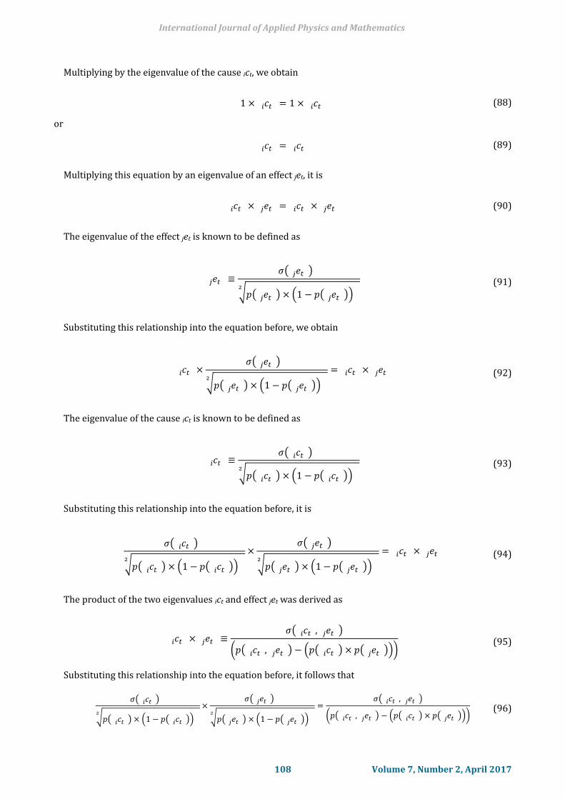
Multiplying by the eigenvalue of the cause ict, we obtain

1 × 𝑐𝑡𝑖 = 1 × 𝑐𝑡𝑖 (88)

or

𝑐𝑡𝑖 = 𝑐𝑡𝑖 (89)

Multiplying this equation by an eigenvalue of an effect jet, it is

𝑐𝑡 ×𝑖 𝑒𝑡𝑗 = 𝑐𝑡 ×𝑖 𝑒𝑡𝑗 (90)

The eigenvalue of the effect jet is known to be defined as

𝑒𝑡𝑗 ≡𝜎( 𝑒𝑡𝑗 )

√𝑝( 𝑒𝑡𝑗 ) × (1 − 𝑝( 𝑒𝑡𝑗 ))2

(91)

Substituting this relationship into the equation before, we obtain

𝑐𝑡 ×𝑖

𝜎( 𝑒𝑡𝑗 )

√𝑝( 𝑒𝑡𝑗 ) × (1 − 𝑝( 𝑒𝑡𝑗 ))2

= 𝑐𝑡 ×𝑖 𝑒𝑡𝑗 (92)

The eigenvalue of the cause ict is known to be defined as

𝑐𝑡𝑖 ≡

𝜎( 𝑐𝑡𝑖 )

√𝑝( 𝑐𝑡𝑖 ) × (1 − 𝑝( 𝑐𝑡𝑖 ))2

(93)

Substituting this relationship into the equation before, it is


√𝑝( 𝑐𝑡𝑖 ) × (1 − 𝑝( 𝑐𝑡𝑖 ))2

×𝜎( 𝑒𝑡𝑗 )

√𝑝( 𝑒𝑡𝑗 ) × (1 − 𝑝( 𝑒𝑡𝑗 ))2

= 𝑐𝑡 ×𝑖 𝑒𝑡𝑗 (94)

The product of the two eigenvalues ict and effect jet was derived as

𝑐𝑡𝑖 × 𝑒𝑡𝑗 ≡

𝜎( 𝑐𝑡𝑖 , 𝑒𝑡𝑗 )


Substituting this relationship into the equation before, it follows that


√𝑝( 𝑐𝑡𝑖 ) × (1 − 𝑝( 𝑐𝑡𝑖 ))2

×𝜎( 𝑒𝑡𝑗 )

√𝑝( 𝑒𝑡𝑗 ) × (1 − 𝑝( 𝑒𝑡𝑗 ))2

=𝜎( 𝑐𝑡𝑖 , 𝑒𝑡𝑗 )




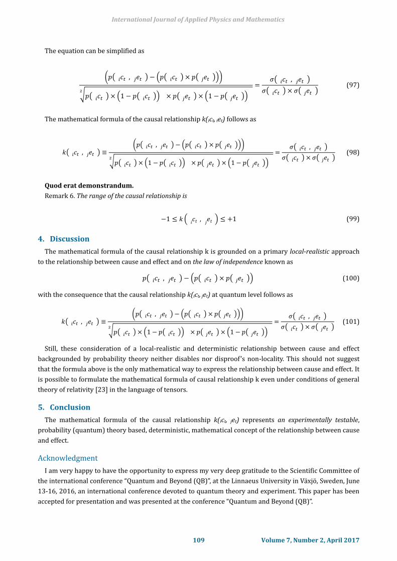
The equation can be simplified as

(𝑝( 𝑐𝑡𝑖 , 𝑒𝑡𝑗 ) − (𝑝( 𝑐𝑡𝑖 ) × 𝑝( 𝑒𝑡𝑗 )))

√𝑝( 𝑐𝑡𝑖 ) × (1 − 𝑝( 𝑐𝑡𝑖 )) × 𝑝( 𝑒𝑡𝑗 ) × (1 − 𝑝( 𝑒𝑡𝑗 ))2


𝜎( 𝑐𝑡𝑖 ) × 𝜎( 𝑒𝑡𝑗 ) (97)

The mathematical formula of the causal relationship k(ict, iet) follows as




𝜎( 𝑐𝑡𝑖 ) × 𝜎( 𝑒𝑡𝑗 ) (98)


Remark 6. The range of the causal relationship is

−1 ≤ 𝑘 ( 𝑐𝑡𝑖 , 𝑒𝑡𝑗 ) ≤ +1 (99)

4. Discussion

The mathematical formula of the causal relationship k is grounded on a primary local-realistic approach

to the relationship between cause and effect and on the law of independence known as

𝑝( 𝑐𝑡𝑖 , 𝑒𝑡𝑗 ) − (𝑝( 𝑐𝑡𝑖 ) × 𝑝( 𝑒𝑡𝑗 )) (100)

with the consequence that the causal relationship k(ict, jet) at quantum level follows as




𝜎( 𝑐𝑡𝑖 ) × 𝜎( 𝑒𝑡𝑗 ) (101)

Still, these consideration of a local-realistic and deterministic relationship between cause and effect

backgrounded by probability theory neither disables nor disproof’s non-locality. This should not suggest

that the formula above is the only mathematical way to express the relationship between cause and effect. It

is possible to formulate the mathematical formula of causal relationship k even under conditions of general

theory of relativity [23] in the language of tensors.

5. Conclusion

The mathematical formula of the causal relationship k(ict, jet) represents an experimentally testable,

probability (quantum) theory based, deterministic, mathematical concept of the relationship between cause

and effect.

Acknowledgment

I am very happy to have the opportunity to express my very deep gratitude to the Scientific Committee of

the international conference “Quantum and Beyond (QB)”, at the Linnaeus University in Växjö, Sweden, June

13-16, 2016, an international conference devoted to quantum theory and experiment. This paper has been

accepted for presentation and was presented at the conference “Quantum and Beyond (QB)”.



References

[1] Heisenberg, W. (1927). Über den anschaulichen Inhalt der quantentheoretischen Kinematik and

Mechanik. Zeitschrift für Physik, 43, 197.

[2] Bohr, N. (1950). On the notions of causality and complementarity. Science, 111, 51-54.

[3] Bohr, N. (1937). Causality and complementarity. Philosophy of Science, 4, 291.

[4] Barukčić, I. (2011). Anti Heisenberg — Refutation of Heisenberg's uncertainty relation. American

Institute of Physics-Conference Proceedings, 322.

[5] Barukčić, I. (2014). Anti Heisenberg — Refutation of Heisenberg's uncertainty principle. International

Journal of Applied Physics and Mathematics, 4, 244-250.

[6] Barukčić, I. (2016). Anti Heisenberg — The end of Heisenberg's uncertainty principle. Journal of Applied

Mathematics and Physics, 4, 881-887.

[7] Barukčić, I. (2016). The mathematical formula of the causal relationship k. International Journal of

Applied Physics and Mathematics, 6, 45-65.

[8] Aharonov, Y., Anandan, J., & Vaidman, L. (1993). Meaning of the wave function. Physical Review A

(Atomic, Molecular, and Optical Physics), 47, 4616-4626.

[9] Barukčić, I. (2016). Anti aristotle — The division of zero by zero. Journal of Applied Mathematics and

Physics, 4, 749-761.

[10] Born, M. (1926). Zur Quantenmechanik der Stoßvorgänge. Zeitschrift für Physik, 37, 363-367.

[11] Barukčić, I. (2016). The physical meaning of the wave function. Journal of Applied Mathematics and

Physics, 4, 988-1023.

[12] Heisenberg, W. (1927) Über den anschaulichen Inhalt der quantentheoretischen Kinematik und

Mechanik. Zeitschrift für Physik, 43, 183.

[13] Barukčić, I. (1989). Die Kausalität, (First German Edition). Hamburg: Wissenschaftsverlag. 218.

[14] Barukčić, I. (1997). Die Kausalität. (Second German Edition). Wilhelmshaven: Scientia. 374.

[15] Barukčić, I. (2005). Causality. New Statistical Methods. (First English Edition). Hamburg: Books on Demand.

488.

[16] Barukčić, I. (2006). Causality. New Statistical Methods. (Second English Edition). Hamburg: Books on

Demand. 488.

[17] Thompson, M. E. (2006). Reviews. Causality. New statistical methods. International Statistical Institute, 26(1),

6.

[18] Barukčić, I. (2006). New method for calculating causal relationships. Proceedings of XXIIIrd International

Biometric Conference.

[19] Barukčić, I. (2006). Causation and the law of independence. Proceedings of Symposium on Causality 2006.

[20] Barukčić, I. (2011). Causality I. A Theory of Energy, Time and Space. Morrisville: Lulu. 648.

[21] Barukčić, I. (2011). Causality II. A Theory of Energy, Time and Space. Morrisville: Lulu. 376.

[22] Barukčić, I. (2012). The deterministic relationship between cause and effect. Proceedings of

International Biometric Conference.

[23] Barukčić, I. (2016) Unified field theory. Journal of Applied Mathematics and Physics, 4(8), 1379-1438.

Ilija Barukčić was born on October 1th, 1961 in Novo Selo (Bosina and Hercegovina,

former Yugoslavia). Barukčić studied at the University of Hamburg, Germany (1982-1989)

human medicine (philosophy and physics). He graduated at the University of Hamburg,

Germany with the degree: State exam. Barukčić’s basic field of research is the relationship

between cause and effect under conditions of quantum and relativity theory, in biomedical

sciences, in philosophy et cetera.



Thus far, among his several publications in physics are the refutation of Heisenberg’s uncertainty

principle (Ilija Barukčić, “Anti Heisenberg - Refutation Of Heisenberg's Uncertainty Relation,” American

Institute of Physics - Conference Proceedings, Volume 1327, pp. 322-325, 2011), the refutation of Bell’s

theorem and the CHSH inequality (Ilija Barukčić, “Anti-Bell - Refutation of Bell's theorem,” American

Institute of Physics - Conference Proceedings, Volume 1508, pp. 354-358, 2012). In another publication,

Barukčić was able to provide the proof that time and gravitational field are equivalent (Ilija Barukčić,

“The Equivalence of Time and Gravitational Field,” Physics Procedia, Volume 22, pp. 56-62, 2011). Barukčić

solved the long lasting problem of the particle and the wave (Ilija Barukčić, "The Relativistic Wave

Equation," International Journal of Applied Physics and Mathematics vol. 3, no. 6, pp. 387-391, 2013.) and

refuted Heisenberg’s uncertainty once again in general (Ilija Barukčić, "Anti Heisenberg – Refutation of

Heisenberg’s Uncertainty Principle," International Journal of Applied Physics and Mathematics vol. 4, no. 4,

pp. 244-250, 2014.). Barukčić was able to provide a mathematical proof that neither Einstein’s cosmological

constant (Ilija Barukčić, "Anti Einstein – Refutation of Einstein’s General Theory of Relativity,"

International Journal of Applied Physics and Mathematics vol. 5, no. 1, pp. 18-28, 2015.) nor Newton’s

gravitational constant (Ilija Barukčić, "Anti Newton — Refutation of the Constancy of Newton's

Gravitational Constant Big G," International Journal of Applied Physics and Mathematics vol. 5, no. 2, pp.

126-136, 2015.) are constant.



Documents

Anti Bohr Quantum Theory and Causality - Semantic Scholar · principle of causality will expel any kind of mysticism from physics and enable a quantization of the . gravitational