1

Case Selection and Causal Inference in Qualitative Research

Thomas Plümpera, Vera E. Troegerb, and Eric Neumayerc

a Department of Government, University of Essex, Wivenhoe Park, ColchesterCO4 3SQ, UK

b Department of Economics and CAGE, University of Warwick, Coventry, CV47AL, v.e.troeger@warwick.ac.uk

c Department of Geography and Environment, London School of Economicsand Political Science (LSE), London WC2A 2AE, UK, e.neumayer@lse.ac.uk

Corresponding author: Thomas Plümper.

2

3

Abstract

The validity of causal inferences in qualitative research depends on the selection

of cases. We contribute to current debates on qualitative research designs by using

Monte Carlo simulations to evaluate the performance of different case selection

techniques or algorithms. We show that causal inference from qualitative research

becomes more reliable when researchers select cases from a larger sample, maxi-

mize the variation in the variable of interest, simultaneously minimize variation of

the confounding factors, and ignore all information on the dependent variable. We

also demonstrate that causal inferences from qualitative research become much

less reliable when the variable of interest is strongly correlated with confounding

factors, when the effect of the variable of interest becomes small relative to the

effect of the confounding factors, and when researchers analyze dichotomous de-

pendent variables.

4

1. Introduction

Qualitative research methods are versatile. They can, for example, be used for

theory building, correcting measurement error, discovering missing variables, and

refining the population of relevant cases. They can also be used for making causal

inferences about the effect of variables of interest on potential outcomes and a

better understanding of causal mechanisms.

It is causal effect inferences that we exclusively focus on in this paper. It

is commonly agreed that qualitative methods are perfectly suitable for testing

necessary and sufficient conditions (Braumoeller and Goertz 2000; Seawright

2002; Seawright and Gerring 2007) and there is consensus among qualitative

methodologists that qualitative researchers aim and indeed should aim at making

causal inferences (Collier, Brady and Seawright 2004; Mahoney and Goertz

2006).1

Arguably, however, most data-generating processes social scientists deal

with are not deterministic. At the very least, the vast majority of social

phenomena are not fully determined by the theories social scientists have

suggested. Yet, we believe that the problem is more fundamental: free will or

unobserved genetic predispositions cause variation in social interactions that will

never be fully explained. The presence of stochastic processes is an obvious

problem for a methodology that does not account for errors. However,

surprisingly little is known about the validity of causal inferences based on

qualitative methods when the data-generating process differs from the implicit

1 Many such studies have been published with leading publishers and in leading journals

and their findings rank prominently among the most influential work in the social

sciences. To give but one example: Elinor Ostrom’s Nobel Prize-awarded study of solu-

tions to common pool problems suggests eight “situational variables” shaping the

probability of successful and stable local resource management (Ostrom 1990: 88ff.).

Based on a case study design, Ostrom generalizes her results as general conditions that

determine the ability of actors to overcome commons problems.

5

assumptions qualitative researchers (have to) make.

Employing Monte Carlo (MC) experiments we compare the relative

performance of 11 case selection algorithms which we partly derive from

common practice in comparative case analyses and we also follow suggestions of

qualitative methodologists. We demonstrate that the validity of causal inferences

from qualitative research in the presence of partly stochastic data-generating

processes strongly depends on the case selection criteria and – more specifically –

the case selection algorithm that qualitative researchers rely on in order to select

cases from a larger population. The very best case selection algorithm results in an

estimated average effect that is almost a hundred times closer to the true effect

than the worst algorithm. We also evaluate the conditions on which the validity of

causal inferences from qualitative research depends. We find that the best

selection algorithms make reliable inferences if a) the explanatory variable of

interest exerts a strong influence on the dependent variable relative to random

noise and confounding factors, if b) the variable of interest is not too strongly

correlated with confounding variables and if c) the dependent variable is not

dichotomous. More importantly, while the best algorithms are still fairly reliable

even in the presence of strong stochastic influences on the dependent variable and

other complications, the worst algorithms are highly unreliable even if the

conditions are met under which qualitative research works best. Another

significant result from our MC analyses is that more complicated case selection

algorithms outperform the best simpler algorithms, but not by much. This

promises that qualitative researchers will not endanger causal inferences too much

if they select cases on the basis of simply maximizing variation in the explanatory

variable of interest and minimizing variation in a confounding variable or

variables.

6

To illustrate the implications of our analysis, we apply the full set of

algorithms to an existing study on the lengths of peace (Fortna 2004). Based on a

mixture of quantitative analysis, a qualitative survey of cases as well as a selection

of two cases for in-depth study, Fortna finds that stronger cease-fire agreements,

i.e., agreements that impose stronger constraints on the belligerent parties, result

in longer lasting peace. None of our algorithms selects the cases chosen by Fortna

(2004), who justifies the selection mainly on the basis that these cases provide a

“hard test of the theory” (56), given the “intractable nature of these conflicts”

(57). However, all our selection algorithms support the existence of a small

positive effect of the strengths of cease-fire agreements on peace duration.

Substantively, case comparisons based on our most reliable selection algorithms

suggests that a one-step increase in the strengths of a cease-fire agreement

prolongs subsequent peace by approximately 3.4 months. This result can by-and-

large be confirmed by a regression analysis of the effect of cease-fire agreements

on peace duration. Using statistical methods we find that a one-step increase in

cease-fire agreements prolongs peace by 8 months on average (though the

standard error is large). According to Fortna’s data, the average peace duration

after cease-fire agreements is 222 months. Thus, cease-fire agreements appear to

affect peace duration, but cease-fire agreements hardly determine the difference

between peace and war. We further demonstrate that the results from case

comparisons differ sharply. This demonstrates the importance of using case

selection algorithms which offer reliable results for a large set of data-generating

processes. In other words, case selection matters for inferences.

We start by discussing the challenges faced by scholars wishing to make

causal inferences in the social sciences. We then discuss the comparative

advantages and disadvantages of qualitative research for making such inferences.

7

A better understanding of the relative merits of different case selection rules

within qualitative research is the first step toward an evaluation of the relative

performance of qualitative versus quantitative methods, which we will tackle in

future research. After reviewing the literature on case selection, we therefore

evaluate the performance of eleven selection algorithms with the help of MC

analyses. We then demonstrate the implications of our analysis for an application

to case selection in Fortna (2004). We conclude with advice on how qualitative

researchers should select cases.2

2. Causal Inference and Qualitative Research

Most questions social scientists are interested in are causal in nature. For example,

in order to reduce poverty, scholars need to understand the causal influence of

policy interventions on social and economic outcomes. Causal effects cannot be

directly observed and they cannot be computed from observational data alone.

Rather the identification of causal effects requires some knowledge of the data-

generating process (Pearl 2009: 97).

Making valid causal inferences is the main task of science, but it is far

from a trivial task. Causal inference has four aspects. The first one is the

identification of a causal effect rather than a mere correlation, the second the

identification of the correct causal effect strength, the third is understanding the

mechanisms driving the causal effect, and the fourth is the generalization of

causal findings to a larger set of cases, and ideally to the entire population for

2 We wish to be clear on what we do not do in this paper. First, we refrain from analyzingcase selection algorithms for qualitative research with more than two cases. Note, however, that allmajor results we show here carry over to selecting more than two cases based on a singlealgorithm. However, we do not yet know whether our results carry over to analyses of more thantwo cases when researchers select cases based on different algorithms – a topic we will revisit infuture research. Second, we do not explore algorithms of case selection when researchers areinterested in more than one explanatory variable. The two self-imposed limitations are closelyrelated to each other: because of degrees of freedom researchers need to analyze between 1+2•kand 2k cases (depending on the complexity of their theory) when they are interested in k differentexogenous variables. MC analyses are in principle suited for these questions and we will addressthem in future work.

8

which a causal effect is claimed. Internal validity comprises the first two aspects,

whereas external validity refers to the extent to which a causal effect can be

generalized.

The fundamental challenge to causal inference stems from the fact that

factual observations cannot be compared to counterfactual observations. Causal

inferences therefore require the comparison of different units of analysis at the

same or another point in time or the same unit of analysis at different points in

time. Mere correlation between two factors does not establish that factor x has

caused effect y and estimates of effect strength will be biased if the research

design insufficiently models the underlying process generating the data, but the

absence of a conditional correlation controlling for a plausible model of the data-

generating process at least casts some doubts on the existence of a causal

mechanism.

Second, the identification of a causal effect (e.g., aspirin is the cause for

a reduction in headache) and an unbiased estimate of its strength is not identical to

understanding the causal mechanism driving the effect. The headache does not

disappear because one swallowed a pill. Rather, it disappears because the pill has

an ingredient, salicylic acid, stopping the transmission of the pain signal to the

brain. Aspirin does not eliminate the origin of the pain but rather prevents the

brain from noticing the pain. Thus, identifying causal effects – the pain disappears

-- is distinct from understanding causal mechanisms.3

Causal inferences also imply generalization. Science is hardly interested

3 Unfortunately, causal mechanisms are an infinite regress: knowing that Aspirin reduces

the reception of pain is one thing, understanding why it works is another. In fact, Aspirin

stops the communication of pain to the brain because its molecules attach themselves to

COX-2 enzymes. This connection prevents the enzyme from creating chemical reactions.

Eventually, the infinite regress of causal mechanisms leads to limits of knowledge or to

metaphysical answers.

9

in finding an unbiased causal effect unless scholars believe that the identified

cause-effect chain can be generalized to other cases. Valid generalization requires

external validity, which consists of two aspects: First, researchers need to identify

the population to which the causal effect can be generalized. This population has a

property that makes the generalization valid. Science is interested in this property.

And second, the strengths of the causal effect identified by analyzing the set of

cases in the sample should be very similar to the mean population effect. This is

important to keep in mind, because careful case selection often improves the

identification of causal effects, but at the same time it is likely to introduce

selection bias.

More generally, then, the different requirements for making causal

inferences regularly conflict with each other. If scholars choose certain research

designs that increase internal validity, they may end up reducing external validity

and vice versa. Sometimes the identification of causal effects prevents the

possibility to infer causal mechanisms. Consider the gold standard for establishing

internal validity, randomized controlled trials. In the ideal scenario, the treatment

group and the control group are identical in all confounding factors (at the very

least, confounding factors have to have similar moments in both groups) and the

sample represents the population. If this is not the case, and randomization can

only asymptotically achieve this ideal, then randomized trials do not identify the

true causal effect. The expected ‘bias’ increases if confounding factors become

rare and/or stronger (relative to the effect of interest). Clearly, the rarer a

confounding factor in the sample, the lower the probability that it is evenly

distributed between treatment and control group. In contrast, the bias declines as

the number of independent participants in the randomized trials increases. In other

words, then, randomized trials are not unbiased, they are merely consistent.

10

Perhaps more importantly, experiments create artificial situations that often

prevent researchers from understanding the very nature of causal mechanisms: the

identification of a causal difference between men and women tells us nothing

about the causal mechanism: do the outcomes for women differ because their

education and their experiences differ, because women are genetically different

from men, or because of some unknown interaction effect between education,

experience and genetic differences? The final weak spot of experiments is

external validity. The artificial situation in the laboratory may affect the behavior

of participants, thereby generating deviations from real world behavior of interest.

In addition, often in social science randomized trials the selected samples do not

even aim at representing the population.

Thus, we argue (once again) that science is a collective process and that

a single analysis is very unlikely to identify a causal relation, to identify the true

effect strengths, to identify the causal mechanism, and to identify the property that

defines the population (or at least the population). Keeping this in mind, we now

discuss the contribution of qualitative research to identifying causal effect

strength.

2.1. Correlation is Not Causality: But what about Qualitative Causal Inference?

For decades, qualitative researchers have argued that qualitative methods are

superior to quantitative methods because “correlation does not imply causality”.

The claim is certainly correct if it is understood as meaning “the presence of a

correlation does not prove the existence of a causal effect”. However, this does

not imply that qualitative methods are superior at making causal inferences. The

counter-critique is that “the existence of an effect in qualitative research does not

imply causality”, let alone an unbiased estimate of the strength of a causal effect.

11

The external validity of the qualitative finding will also often be limited. But

under what conditions are quantitative and qualitative causal inferences valid?

To answer this question, one first has to specify whether one uses a

dichotomous or a continuous concept of “validity”. If we apply a dichotomous

concept of validity (inference is either valid or not), then causal effect inference

from quantitative research is valid iff (if and only if) the empirical model perfectly

matches the true data-generating process and estimation is based on a sufficiently

large random sample drawn from the true population. Needless to say, this is

extremely unlikely to hold in reality. If we apply the same dichotomous concept

of validity to causal inference from qualitative research, inferences are valid iff all

confounding factors are identical in all analyzed cases and the analyzed cases

represent the population. As with its quantitative counterpart, existing qualitative

research is not likely to meet these strict conditions.

The failure of existing research designs to satisfy the strict conditions of

a dichotomous definition of validity casts doubt on the practical usefulness and

appeal of this definition. Instead, researchers should aim at maximizing the

internal and external validity with validity defined as a continuous concept. In

other words, one method can allow researchers to make more valid inferences

than other methods, but whether or not a method is superior clearly depends on

the research question. The question thus becomes whether qualitative research is

likely to improve the validity of causal inferences and under which conditions

qualitative research adds insights that other methods are unlikely to bring to the

table.

2.2. The Comparative Advantages and Disadvantages of Qualitative

Research

12

The analysis of selected cases from a sample provides an obvious alternative to

randomization of treatments (as in experiments) or random large-N sampling (as

in standard regression analyses). The major advantage of the analysis of selected

cases over experiments is that qualitative research offers a good chance to link a

causal effect to a causal mechanism, whereas experiments do not tell us much on

the causal mechanism driving the effect. Compared to standard regression

techniques, it becomes questionable, however, whether qualitative methods offer

much of an advantage. In principle, quantitative researchers command over

techniques that allow the estimation of causal mechanisms. Simultaneous equation

models, for example, allow estimating causal chains of decisions and events not

identical to but similar to the way process tracing methods reconstruct causal

mechanisms from observation.

Yet, qualitative research has other comparative advantages and other

disadvantages over regression analyses. Qualitative research has advantages with

respect to internal validity of causal inferences if the stochastic element in the data

is small and if scholars use a reliable selection rule (on which more below). In

cases in which qualitative research identified the true causal effect, they should

then also be able to understand the causal mechanism. Yet, qualitative methods

also have three major weaknesses. First, the selection of cases severely reduces

the representativeness of the sample for the population. Albeit the degree to which

external validity declines depends on the selection algorithm, a small number of

carefully selected cases will never exactly represent the population. External

validity is the comparative advantage of regression analysis. Unless scholars have

wrong perceptions of the underlying population from which they draw a large-N

random sample or they incur strong selection bias in constructing their sample, the

external validity of regression analyses is superior to any other method. Second, if

13

causal heterogeneity exists, for example if the treatment effect is conditional on

confounding factors, qualitative methods will fail to identify the treatment effect.

The same holds if qualitative researchers misspecify confounding factors. If not

all confounding factors are accounted for, the observed causal effect will be

biased and thus reduce the validity of causal inferences. Finally, qualitative

methods do not account for stochastic processes and unsystematic measurement

error. If these factors become large relative to the variance explained by structural

factors, inferences from qualitative research become unreliable.

2.3. Discussion

The most striking of the disadvantages of qualitative research is its inability to

account for stochastic processes and its limited ability to account for other

complications of the data-generating process. However, the degree to which

unaccounted stochastic processes and other model misspecifications invalidate

causal inferences from qualitative research remains unknown. We are not aware

of any research that rigorously studies the relative performance of qualitative

methods in such circumstances.

Such research, we argue, has two ambitions. Ideally one would like to

know the conditions under which quantitative versus qualitative methods have

advantages in identifying or approximating the true causal effect. But before one

can explore this question, which we intend to do in future research, one first has to

understand how the degree to which qualitative research can approximate the true

causal effect crucially depends on the rule for selecting cases. This is what we

study in the remainder of the article. After a review of the literature on case

selection in qualitative research, in the remainder of this paper we therefore

compare the relative performance of eleven different case selection algorithms in

approximating the true causal effect with data-generating processes that include

14

stochastic errors and other complications.

3. Literature Review: Case Selection in Qualitative Research

Methodological advice on the selection of cases in qualitative research stands in a

long tradition. John Stuart Mill in his A System of Logic, first published in 1843,

proposed five methods that were meant to enable researchers to make causal in-

ferences: the method of agreement, the method of difference, the double method

of agreement and difference, the method of residues, and the method of concomi-

tant variation. Modern methodologists have questioned and criticized the useful-

ness and general applicability of Mill’s methods (see, for example, Sekhon 2004).

However, without doubt Mill’s proposals had a major and lasting impact on the

development of the two most prominent modern methods, namely the ‘most

similar’ and ‘most different’ comparative case study designs (Przeworski and Te-

une 1970; Lijphart 1971, 1975; Meckstroth 1975).

Yet, as Seawright and Gerring (2008: 295) point out, these and other

methods of case selection are ‘poorly understood and often misapplied’. Qualita-

tive researchers mean very different things when they invoke the same terms

‘most similar’ or ‘most different’ and usually the description of their research

design is not precise enough to allow readers to assess how exactly cases have

been chosen. Seawright and Gerring (2008) have therefore provided a formal

definition and classification of these and other techniques of case selection. They

suggest that “in its purest form” (Seawright and Gerring 2008: 304) the ‘most

similar’ design chooses cases which appear to be identical on all controls (z) but

different in the variable of interest (x). Naturally, the ‘most similar’ technique is

not easily applied as researchers find it difficult to match cases such that they are

identical on all control variables. As Seawright and Gerring (2008: 305) concede:

“Unfortunately, in most observational studies, the matching procedure described

15

previously – known as exact matching – is impossible.” This impossibility has

three sources: first, researchers usually do not know the true model. Therefore

they simply cannot match on all control variables. Second, even if known to affect

the dependent variable, many variables remain unobserved. And third, even if all

necessary pieces of information are available, two cases which are identical in all

excluded variables may not be available. Therefore, Lijphart (1975: 163)

suggested a variant of this method that asks researchers to maximize “the ratio

between the variance of the operative variables and the variance of the control

variables”.

Despite ambiguity in its definition and practical operationalization,

qualitative researchers prefer the ‘most similar’ technique over its main rival, the

‘most different’ design. Seawright and Gerring (2008: 306) believe that this

dominance of ‘most similar’ over ‘most different’ design is well justified.

Defining the ‘most different’ technique as choosing two cases that are identical in

the outcome y and the main variable of interest x but different in all control

variables z, they argue that this technique does not generate much leverage.4 They

criticize three points: first, the chosen cases never represent the entire population

(if x can in fact vary in the population). Second, the lack of variation in x renders

it impossible to identify causal effects. And third, elimination of rival hypotheses

is impossible.5 We add that the absence of variation in the control variables does

not imply that specific control variables have no influence on the outcome – it

could also be that the aggregate influences of all confounding factors cancel each

4 As Gerring (2004: 352) formulates poignantly: “There is little point in pursuing cross-unit

analysis if the units in question do not exhibit variation on the dimensions of theoretical

interest and/or the researcher cannot manage to hold other, potentially confounding,

factors constant.”

5 The latter criticism appears somewhat unfair since no method can rule out the possibility

of unobserved confounding factors entirely. Of course, well designed experiments get

closest to ruling out this possibility.

16

other out. Thus, the design cannot guarantee valid inferences and the

generalization to other subsamples appears to be beyond the control of the

selection process.

Seawright and Gerring also identify a third technique for selecting cases in

comparative case studies, which they label the ‘diverse’ technique. It selects cases

so as to “represent the full range of values characterizing X, Y, or some particular

X/Y relationship” (Seawright and Gerring 2008: 300). This definition is

somewhat ambiguous and vague (“some particular relationship”), but one of the

selection algorithms used below in our MC simulations captures the essence of

this technique by simultaneously maximizing variation in y and x.

Perhaps surprisingly, King, Keohane and Verba’s (1994) important

contribution to qualitative research methodology discusses case selection only

from the perspective of unit homogeneity – broadly understood as constant effect

assumption (King et al. 1994: 92)6 – and selection bias – defined as non-random

selection of cases that are not statistically representative of the population (Collier

1995: 462). Selecting cases in a way that does not avoid selection bias negatively

affects the generalizability of inferences. Random sampling from the population

of cases would clearly avoid selection bias. Thus, given the prominence of

selection bias in King et al.’s discussion of case selection, the absence of random

sampling in comparative research may appear surprising. But it is not. Random

selection of cases leads to inferences which are correct on average when the

number of conducted case studies approaches infinity, but the sampling deviation

is extremely large. As a consequence, the reliability of single studies of randomly

6 This interpretation deviates from Holland’s definition of unit homogeneity, which

requires that the conditional effect and the marginal effect are identical, implying that the

size of the independent variable is the same (Holland 1986: 947). To satisfy King et al.’s

definition of unit homogeneity, only the marginal effect has to be identical (King et al.

92-93).

17

sampled cases remains low. The advice King and his co-authors give on case

selection, then, lends additional credibility to common practices chosen by applied

qualitative researchers, namely to avoid truncation of the dependent variable (p.

130, see also Collier et al. 2004: 91), to avoid selection on the dependent variable

(p. 134, see also Collier et al. 2004: 88), while at the same time selecting

according to the categories of the ‘key causal explanatory variable’.7

To conclude, while there is a growing consensus on the importance of case

selection for social science research in general and qualitative research in

particular, as yet very little overall agreement has emerged concerning the use of

central terminology and the relative advantages of different case selection

mechanisms. Scholars agree that random sampling is unsuitable for qualitative

research, but disagreement on sampling on the dependent variable and the

appropriate use of information from potentially observed confounding factors

persists. In the next sections, we first discuss the use of MC experiments for

evaluating case selection mechanisms in qualitative research. We then identify

and characterize the selection algorithms we compare, report the assumptions we

make in the MC study and discuss the results.

4. Case Selection Algorithms

With respect to the case selection algorithms employed, we attempt to be as

comprehensive as necessary. We cover selection rules (algorithms as we prefer to

call them to highlight the deterministic character of case selection) commonly

used in applied research, but also various simple permutations and extensions. As

7 King et al. (1994) also repeatedly claim that increasing the number of observations makes

causal inferences more reliable. Qualitative researchers have argued that this view, while

correct in principle, does not do justice to qualitative research (Brady 2004, Bartels 2004,

McKeown 2004). More importantly, they also suggest that the extent to which the logic

of quantitative research can be superimposed on qualitative research designs has limits.

18

mentioned already, we assume without loss of generality a data generating process

in which the dependent variable y is a linear function of a variable of interest x, a

control variable z and an error term ε.8 Ignoring for the time being standard advice

against sampling on the dependent variable, researchers might wish to maximize

variation of y, maximize variation of x, minimize variation of z or some

combination thereof. Employing the two most basic functions to aggregate infor-

mation on more than one variable, namely addition and subtraction, this leads to

seven permutations of information to choose from, which together with random

sampling results in eight simple case selection algorithms – see table 1. The

mathematical description of the selection algorithms, as shown in the last column

of the table, relies on the set-up of the MC analyses (described in the next

section). In general, for each variable we generate Euclidean distance matrices,

which is an N×N matrix representing the difference or distance in a set of case-

dyads ij. Naturally, we only consider the off-diagonals (we suppress the case dyad

ii) since a comparison of an observation to itself would not allow inference.

Starting from these distance matrices, we select two cases that maximize (or

minimize) a selection rule. For example, max(x) only considers the explanatory

variable of interest, thereby ignoring the distance matrices for the dependent

variable y and the control vector Z. With max(x), we select the two cases that

represent the cell of the distance matrix with the largest distance value.

8 Since we can interpret z as a vector of k control variables, we can generalize findings to

analyses with multiple controls. However, we cannot generalize to selection algorithms

that select two cases on one dimension and two other cases on another dimension of

controls. We leave these issues to future research.

19

Table 1: Simple Case Selection Algorithms

sampling informationName max

dist(y)max

dist(x)min

dist(z)selection algorithm

1 Random no no no random draw2 max(y) yes no no max dist(y)3 max(x) no yes no max dist(x)4 min(z) no no yes min dist(z)5 max(y)max(x) yes yes no max [dist(y)+dist(x)]6 max(y)min(z) yes no yes max [dist(y)-dist(z)]7 max(x)min(z) no yes yes max [dist(x)-dist(z)]8 max(y)max(x)min(z) yes yes yes max [dist(y)+dist(x)-dist(z)]

Algorithm 1 does not use information (other than that a case belongs to the popu-

lation) and thus randomly samples cases. We include this algorithm for complete-

ness and because qualitative methodologists argue that random sampling – the

gold standard for simulations and quantitative research – does not work well in

small-N comparative research (Seawright and Gerring 2008: 295; King et al.

1994: 124), unless it is used for choosing cases for closer study as a complement

to large-N quantitative research (Fearon and Laitin 2008).

We incorporate the second algorithm – pure sampling on the dependent

variable without regard to variation of either x or z – for the same completeness

reason. Echoing Geddes (1990), many scholars have argued that sampling on the

dependent variable biases the results (King et al. 1994: 129, Collier and Mahoney

1996, Collier et al. 2004: 99). Geddes demonstrates that ‘selecting on the depend-

ent variable’ lies at the core of invalid results generated from qualitative research

in fields as diverse as economic development, social revolution, and inflation.

But does Geddes’s compelling critique of sampling on the dependent

variable imply that applied researchers should entirely ignore information on the

dependent variable when they also use information on the variable of interest or

the confounding factors? Algorithms 5, 6, and 8 help us to explore this question.

These rules include selection on the dependent variable in addition to selection on

20

x and/or z. Theoretically, these algorithms should perform better than the

algorithm 2, but we are more interested in analyzing how these biased algorithms

perform in comparison to their counterparts, namely algorithms 3, 4, and 7,

which, respectively, maximize variation of x, minimize variation of z and simulta-

neously maximize variation of x and minimize variation of z, just as algorithms 5,

6 and 8 do, but this time without regard to variation of y.

Theoretically, one would expect algorithm 7 to outperform algorithms 3

and 4. Qualitative methodologists such as Gerring (2007) and Seawright and Ger-

ring (2008) certainly expect this outcome and we concur. Using more information

must be preferable to using less information when it comes to sampling. This does

not imply, however, that algorithm 7 necessarily offers the optimal selection rule

for comparative qualitative research. Since information from at least two different

variables has to be aggregated, researchers have multiple possible algorithms at

their disposal that all aggregate information in different ways. For example, in

addition to the simple unweighted sum (or difference) that we assume in table 1,

one can aggregate by multiplying or dividing the distances and one can also

weight the individual components.9

An alternative function for aggregation has in fact been suggested by

Arend Lijphart (1975), namely maximizing the ratio of the variance in x and z:

max[dist(x)/dist(z)]. We include Lijphart’s suggestion as our algorithm 9 even

though it suffers from a simple problem which reduces its usefulness: when the

variance of the control variable z is smaller than 1.0, the variance of what Lijphart

calls the operative variable x becomes increasingly unimportant for case selection

(unless of course the variation of the control variables is very similar across dif-

ferent pairs of cases). We solve this problem by also including in the competition

9 Other functions for aggregating information such as logarithms, roots and so on are of

course possible.

21

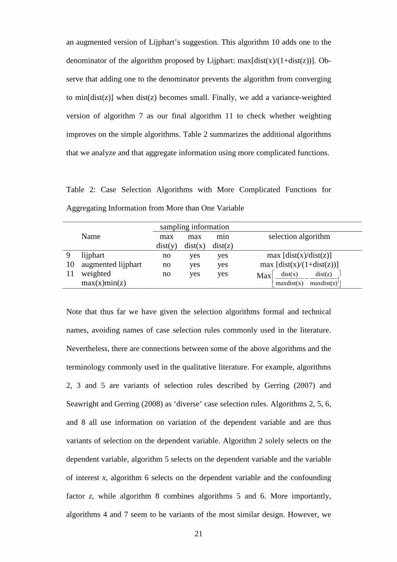
an augmented version of Lijphart’s suggestion. This algorithm 10 adds one to the

denominator of the algorithm proposed by Lijphart: max[dist(x)/(1+dist(z))]. Ob-

serve that adding one to the denominator prevents the algorithm from converging

to min[dist(z)] when dist(z) becomes small. Finally, we add a variance-weighted

version of algorithm 7 as our final algorithm 11 to check whether weighting

improves on the simple algorithms. Table 2 summarizes the additional algorithms

that we analyze and that aggregate information using more complicated functions.

Table 2: Case Selection Algorithms with More Complicated Functions for

Aggregating Information from More than One Variable

sampling informationName max

dist(y)max

dist(x)min

dist(z)selection algorithm

9 lijphart no yes yes max [dist(x)/dist(z)]10 augmented lijphart no yes yes max [dist(x)/(1+dist(z))]11 weighted

max(x)min(z)no yes yes Max dist(x) dist(z)

maxdist(x) maxdist(z)

Note that thus far we have given the selection algorithms formal and technical

names, avoiding names of case selection rules commonly used in the literature.

Nevertheless, there are connections between some of the above algorithms and the

terminology commonly used in the qualitative literature. For example, algorithms

2, 3 and 5 are variants of selection rules described by Gerring (2007) and

Seawright and Gerring (2008) as ‘diverse’ case selection rules. Algorithms 2, 5, 6,

and 8 all use information on variation of the dependent variable and are thus

variants of selection on the dependent variable. Algorithm 2 solely selects on the

dependent variable, algorithm 5 selects on the dependent variable and the variable

of interest x, algorithm 6 selects on the dependent variable and the confounding

factor z, while algorithm 8 combines algorithms 5 and 6. More importantly,

algorithms 4 and 7 seem to be variants of the most similar design. However, we

22

do not call any of these algorithms ‘selection on the dependent variable’ or ‘most

similar’. The reason is that, as discussed above, there is a lack of consensus on

terminology and different scholars prefer different labels and often mean different

things when they invoke rules such as ‘sampling on the dependent variable’ or

‘most similar’.

We conclude the presentation and discussion of case selection algorithms

with a plea for clarity and precision. Rather than referring to a ‘case selection

design’, qualitative researchers should be as clear and precise as possible when

they describe how they selected cases. Qualitative research will only be replicable

if scholars provide information on the sample from which they selected cases, the

variables of interest and the confounding factors, and the selection algorithm they

used. Others can only evaluate the validity of causal inferences if qualitative

researchers provide all this information.

5. Monte Carlo Experiments

We use the standard tool of quantitative methodologists to compare estimators –

MC simulations – to explore the reliability of case selection in qualitative

research. This analysis explores whether a comparison of two cases allows

researchers to identify the effect that one explanatory variable, called x, exerts on

a dependent variable, called y. We assume that this dependent variable y is a

function of x, a single control variable z, which is observed, and some error term

ε.10 There are different ways to think about this error term. First, scientists usually

implicitly assume that the world is not perfectly determined and allow multiple

10 We follow the convention of quantitative methodology and assume that the error term is

randomly drawn from a standard normal distribution. Note, however, that since we are

not interested in asymptotic properties of case selection algorithms, we could as well

draw the error term from different distributions. This would have no consequence other

than adding systematic bias to all algorithms alike.

23

equilibria which depend on random constellations or the free will of actors. In this

respect, the error term accounts for the existence of randomness. Second, virtually

all social scientists acknowledge the existence of systematic and unsystematic

measurement error. The error term can be perceived as accounting for information

which is partly uncertain. And third, the error term can be interpreted as model

uncertainty, that is, as unobserved omitted variables also exerting an influence on

the dependent variable. Only if randomness and free will, measurement error, and

model uncertainty did not exist, would the inclusion of an error term make no

sense.

MC simulations provide insights into the expected accuracy of

inferences given certain pre-defined properties of the data-generating process.

They are used to discriminate between two or more methodologies (i.e. estimation

techniques, sampling rules, and so on). Starting from there, researchers can

systematically change the data-generating process and explore the comparative

advantages of different methodologies. Possible systematic changes include

variation in the assumed level of correlation between explanatory variables, the

relative importance of uncertainty, the level of measurement error, and so on.

Unsystematic changes are modeled by repeated random draws of the error term.

These changes allow to systematically compare the ex ante reliability of the

inferences based on different selection algorithms and thus their relative

performance, which is what we are interested in.

Specifically, we define various data generating processes from which we

draw a number of random samples and then select two cases from each sample

according to a specific algorithm, as defined in the previous section. As a

consequence of the unaccounted error process, the computed effects from the

various Monte Carlo simulations will deviate somewhat from the truth. Yet, since

24

we confront all selection algorithms with the same set of data generating

processes, including the same error processes, performance differences must

result from the algorithms themselves. These differences occur because different

algorithms will select different pairs of cases i and j and as a consequence, the

computed effect and the distance of this effect from the true effect differs.

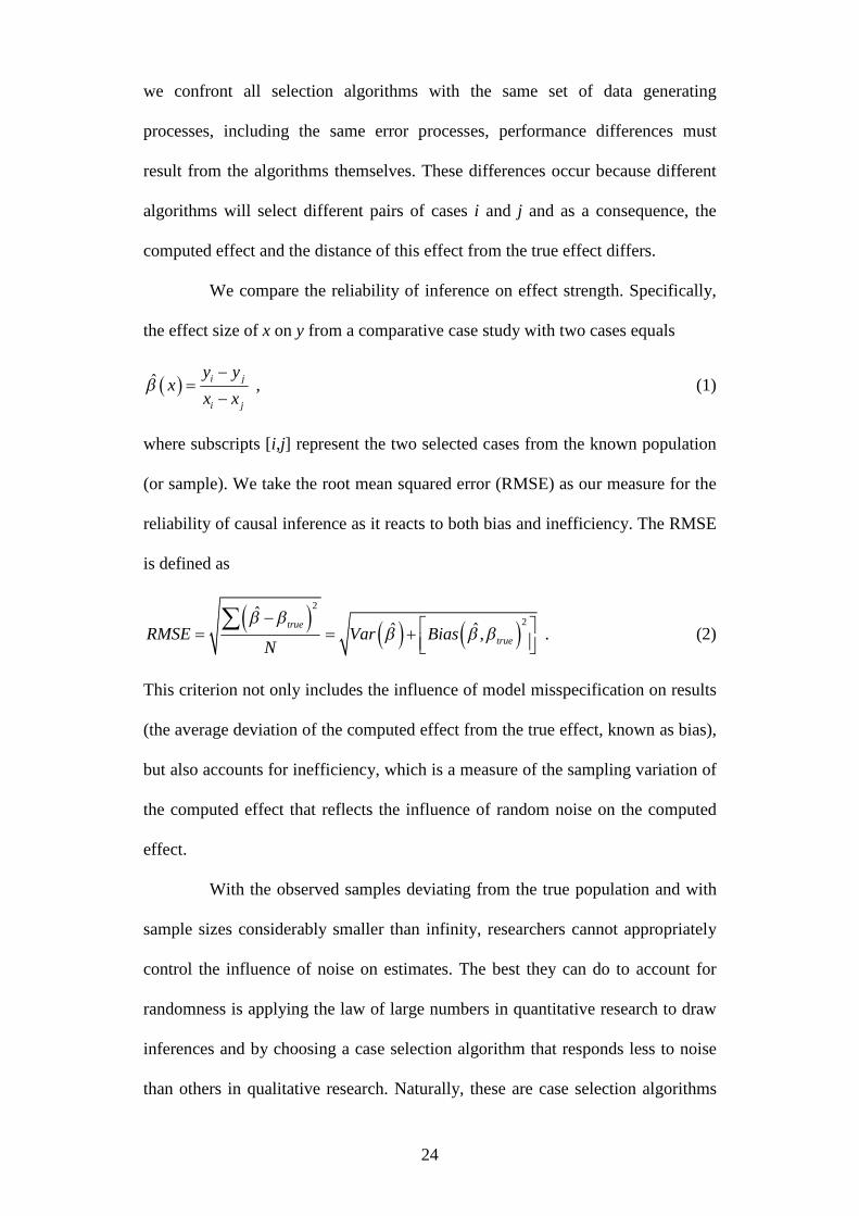
We compare the reliability of inference on effect strength. Specifically,

the effect size of x on y from a comparative case study with two cases equals

ˆ i j

i j

y yx

x x

, (1)

where subscripts [i,j] represent the two selected cases from the known population

(or sample). We take the root mean squared error (RMSE) as our measure for the

reliability of causal inference as it reacts to both bias and inefficiency. The RMSE

is defined as

2

2ˆ

ˆ ˆ,true

trueRMSE Var BiasN

. (2)

This criterion not only includes the influence of model misspecification on results

(the average deviation of the computed effect from the true effect, known as bias),

but also accounts for inefficiency, which is a measure of the sampling variation of

the computed effect that reflects the influence of random noise on the computed

effect.

With the observed samples deviating from the true population and with

sample sizes considerably smaller than infinity, researchers cannot appropriately

control the influence of noise on estimates. The best they can do to account for

randomness is applying the law of large numbers in quantitative research to draw

inferences and by choosing a case selection algorithm that responds less to noise

than others in qualitative research. Naturally, these are case selection algorithms

25

that use more information. In quantitative research, the property characterizing the

best use of information is called efficiency and we see no reason to deviate from

this terminology.

We conducted Monte Carlo simulations with both a continuous and a

binary dependent variable. As one would expect, the validity of inferences is

significantly lower with a binary dependent variable, since binary variables

provide less information. Since otherwise results are substantively identical we

only report in detail the findings from the simulations with a continuous

dependent variable here; results for the simulations with the dichotomous

dependent variable are briefly summarized and details can be found in the

appendix. We use a simple linear cross-sectional data generating process for

evaluating the relative performance of case selection algorithms in qualitative

research:

i i i iy x z , (3)

where y is the dependent variable, x is the exogenous explanatory variable of in-

terest, z is a control variable, , represent coefficients and is an iid error

process. This data generating process resembles what Gerring and McDermott

(2007: 690) call a ‘spatial comparison’ (a comparison across n observations), but

our conclusions equally apply to ‘longitudinal’ (a comparison across t periods)

and ‘dynamic comparisons’ (a comparison across n·t observations).

The variables x and z are always drawn from a standard normal distribu-

tion. Given the low number of observations, it comes without loss in generality

that we draw from a normal distribution with mean zero and standard deviation

of 1.511, and, unless otherwise stated, all true coefficients take the value of 1.0, the

11 Thereby, we keep the R² at appr. 0.5 for the simulations with a continuous dependent

variable.

26

standard deviation of variables is 1.0, correlations are 0.0 and the number of

observations N equals 100.

Once we have generated y, x and z based on our simple data generating

process as described above, we apply our 11 case selection algorithms to select to

cases from which we compute the effect of x on y. In general we generate

Euclidean distance matrices for each of the three variables which give the

difference or distance between each two cases for y, x and z. We then select two

cases for each selection algorithm, e.g. for algorithm 2 “max dist(y)” we select the

two cases which have the largest Euclidian distance with respect to y. In the case

of algorithm 5 "max [dist(y)+dist(x)]" we choose the pair of cases that maximizes

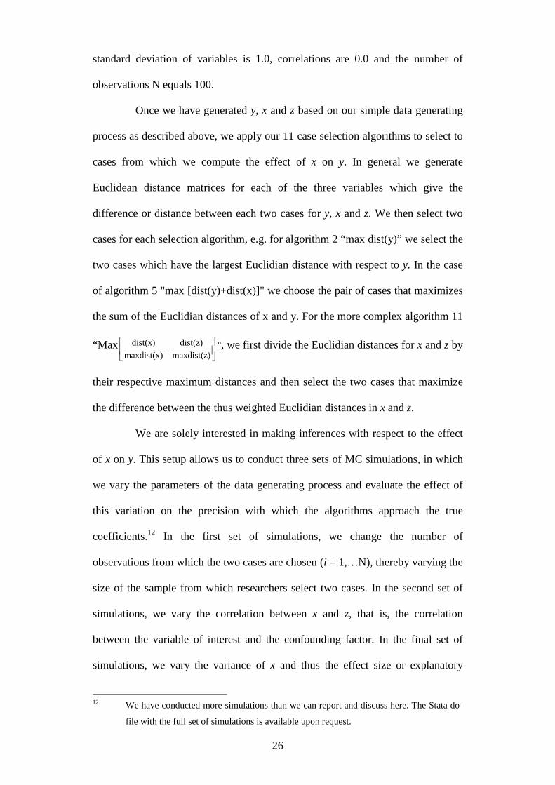
the sum of the Euclidian distances of x and y. For the more complex algorithm 11

“Max dist(x) dist(z)

maxdist(x) maxdist(z)

”, we first divide the Euclidian distances for x and z by

their respective maximum distances and then select the two cases that maximize

the difference between the thus weighted Euclidian distances in x and z.

We are solely interested in making inferences with respect to the effect

of x on y. This setup allows us to conduct three sets of MC simulations, in which

we vary the parameters of the data generating process and evaluate the effect of

this variation on the precision with which the algorithms approach the true

coefficients.12 In the first set of simulations, we change the number of

observations from which the two cases are chosen (i = 1,…N), thereby varying the

size of the sample from which researchers select two cases. In the second set of

simulations, we vary the correlation between x and z, that is, the correlation

between the variable of interest and the confounding factor. In the final set of

simulations, we vary the variance of x and thus the effect size or explanatory

12 We have conducted more simulations than we can report and discuss here. The Stata do-

file with the full set of simulations is available upon request.

27

power of x relative to the effect size of the confounding factor z.

Analyzing the impact of varying the sample size on the validity of infer-

ence in qualitative research may seem strange at first glance. After all, qualitative

researchers usually study a fairly limited number of cases. In fact, in our MC

analyses we generate effects by looking at a single pair of cases selected by each

of the case selection algorithms. So why should the number of observations from

which we select the two cases matter? The reason is that if qualitative researchers

can choose from a larger number of cases about which they have theoretically

relevant information, they will be able to select a better pair of cases given the

chosen algorithm. The more information researchers have before they select cases

the more reliable their inferences should thus become.

By varying the correlation between x and the control variable z we can

analyze the impact of confounding factors on the performance of the case

selection algorithms. With increasing correlation, inferences should become less

reliable. Thereby, we go beyond the usual focus on ‘sampling error’ of small-N

studies and look at the effect of potential model misspecification on the validity of

inference in qualitative research. While quantitative researchers can eliminate the

potential for bias from correlated control variables by including these on the right-

hand-side of the regression model, qualitative researchers have to use appropriate

case selection rules to reduce the potential for bias.

Finally, in varying the standard deviation of x we analyze the impact of

varying the strength of the effect of the variable of interest on the dependent vari-

able. The larger this relative effect size of the variable of interest, the more reli-

able causal inferences should become.13 The smaller the effect of the variable of

13 We achieve this by changing the variance of the explanatory variable x, leaving the

variance of the confounding factor z and the coefficients constant. Equivalently, one

28

interest x on y in comparison to the effect of the control or confounding variables

z on y, the harder it is to identify the effect correctly and the less valid the infer-

ences, especially when the researcher does not know the true specification of the

model.

6. Results

We now turn to reporting the results of the three sets of MC analyses, i.e. in which

we vary the sample size N, vary the correlation between x and the confounding

factor z, and vary the standard deviation of x. For the simple linear data generating

process, these three variations mirror the most important factors that can influence

the inferential performance of case selection algorithms. In each type of analysis

we draw 1000 samples from the underlying data generating process. Table 3

reports the Monte Carlo results where we only vary the size of the sample from

which we draw the two cases we compare. In this simulation, we do not allow for

systematic correlation between the variable of interest x and the confounding

factor z. The deviations of computed effects from the true effect occur because of

‘normal’ sampling error and how efficiently the algorithm deals with the available

information.

could leave the variance of x constant and vary the variance of z. Alternatively, one can

leave both variances constant and change the coefficients of x and/or z.

29

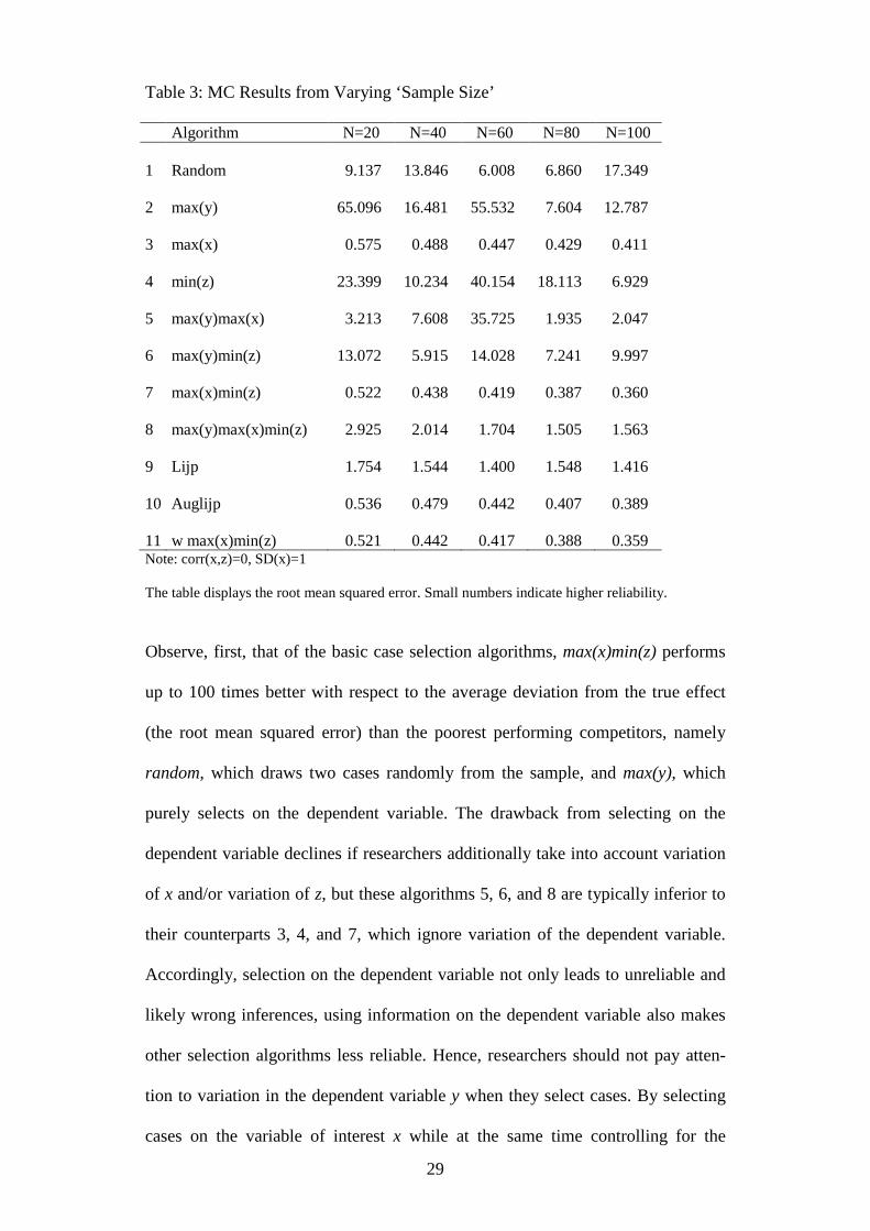
Table 3: MC Results from Varying ‘Sample Size’

Algorithm N=20 N=40 N=60 N=80 N=100

1 Random 9.137 13.846 6.008 6.860 17.349

2 max(y) 65.096 16.481 55.532 7.604 12.787

3 max(x) 0.575 0.488 0.447 0.429 0.411

4 min(z) 23.399 10.234 40.154 18.113 6.929

5 max(y)max(x) 3.213 7.608 35.725 1.935 2.047

6 max(y)min(z) 13.072 5.915 14.028 7.241 9.997

7 max(x)min(z) 0.522 0.438 0.419 0.387 0.360

8 max(y)max(x)min(z) 2.925 2.014 1.704 1.505 1.563

9 Lijp 1.754 1.544 1.400 1.548 1.416

10 Auglijp 0.536 0.479 0.442 0.407 0.389

11 w max(x)min(z) 0.521 0.442 0.417 0.388 0.359Note: corr(x,z)=0, SD(x)=1

The table displays the root mean squared error. Small numbers indicate higher reliability.

Observe, first, that of the basic case selection algorithms, max(x)min(z) performs

up to 100 times better with respect to the average deviation from the true effect

(the root mean squared error) than the poorest performing competitors, namely

random, which draws two cases randomly from the sample, and max(y), which

purely selects on the dependent variable. The drawback from selecting on the

dependent variable declines if researchers additionally take into account variation

of x and/or variation of z, but these algorithms 5, 6, and 8 are typically inferior to

their counterparts 3, 4, and 7, which ignore variation of the dependent variable.

Accordingly, selection on the dependent variable not only leads to unreliable and

likely wrong inferences, using information on the dependent variable also makes

other selection algorithms less reliable. Hence, researchers should not pay atten-

tion to variation in the dependent variable y when they select cases. By selecting

cases on the variable of interest x while at the same time controlling for the

30

influence of confounding factors, researchers are likely to choose cases which

vary in their outcome if x indeed exerts an effect on y.

Maximizing variation of x while at the same time minimizing variation

of z appears optimal. Algorithm 7 uses subtraction as a basic function for

aggregating information from more than one variable. Would using a more

complicated function dramatically improve the performance of case selection?

Results reported in table 3 show that, at least for this set of simulations, this is not

the case. Algorithm 7 performs roughly 10 percent better than the augmented

version of Lijphart’s proposal (auglijp) and while algorithm 11, the variance-

weighted version of algorithm 7, is very slightly superior, not much separates the

performance of the two.

Another interesting finding from table 3 is that only four algorithms be-

come systematically more reliable when the sample size increases from which we

draw two cases: max(x), max(x)min(z) and its weighted variant w max(x)min(z), as

well as auglijp. Of course, algorithms need to have a certain quality to generate vi-

sible improvements when the sample size becomes larger. Random selection, for

example, only improves on average if the increase in sample size leads to relati-

vely more ‘onliers’ than ‘outliers’. This may be the case, but there is no guarantee.

When researchers use relatively reliable case selection algorithms, however, an

increase in the size of the sample, on which information is available, improves

causal inferences unless one adds extreme outliers to the sample.14 In fact,

extreme outliers are problematic for causal inferences from comparative case

analysis. They therefore should be excluded from the sample from which

14 Note, we say that inferences become more reliable if cases are selected from a larger

sample of cases for which researchers have sufficient information. We are not making any

normative claim about enlarging the sample size, because the improvements of enlarging

the sample from which cases are selected has to be discounted by the deteriorations

caused by an increase in case heterogeneity caused by an enlarged sample.

31

researchers select cases. However, researchers can only know whether a case is an

outlier if they know the regression line. Extreme values in one or more variables,

a criterion occasionally employed by qualitative researchers, does not reveal

whether a case is an outlier.

The results so far support the arguments against random selection and

King, Keohane and Verba’s (1994) verdict against sampling on the dependent

variable, but of course qualitative researchers hardly ever select cases randomly.

Selection on the dependent variable may be more common practice, even if re-

searchers rarely admit to it. If researchers know, as they typically do, that both x

and y vary in similar ways and allow this variation to guide their case selection,

then the results are likely to simply confirm their theoretical priors. Selection rules

must thus be strict and should be guided by verifiable rules rather than discretion.

In table 4, we report the results of Monte Carlo simulations from varying

the correlation between the variable of interest x and the confounding factor z.

32

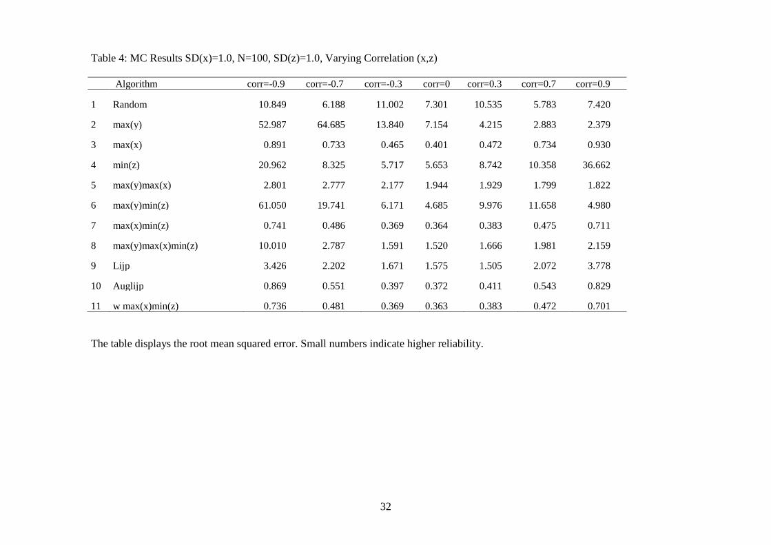
Table 4: MC Results SD(x)=1.0, N=100, SD(z)=1.0, Varying Correlation (x,z)

Algorithm corr=-0.9 corr=-0.7 corr=-0.3 corr=0 corr=0.3 corr=0.7 corr=0.9

1 Random 10.849 6.188 11.002 7.301 10.535 5.783 7.420

2 max(y) 52.987 64.685 13.840 7.154 4.215 2.883 2.379

3 max(x) 0.891 0.733 0.465 0.401 0.472 0.734 0.930

4 min(z) 20.962 8.325 5.717 5.653 8.742 10.358 36.662

5 max(y)max(x) 2.801 2.777 2.177 1.944 1.929 1.799 1.822

6 max(y)min(z) 61.050 19.741 6.171 4.685 9.976 11.658 4.980

7 max(x)min(z) 0.741 0.486 0.369 0.364 0.383 0.475 0.711

8 max(y)max(x)min(z) 10.010 2.787 1.591 1.520 1.666 1.981 2.159

9 Lijp 3.426 2.202 1.671 1.575 1.505 2.072 3.778

10 Auglijp 0.869 0.551 0.397 0.372 0.411 0.543 0.829

11 w max(x)min(z) 0.736 0.481 0.369 0.363 0.383 0.472 0.701

The table displays the root mean squared error. Small numbers indicate higher reliability.

33

Note that all substantive results from table 3 remain valid if we allow for correla-

tion between the variable of interest and the confounding factor. In particular,

algorithm 11, which weights the individual components of the best-performing

simple case selection algorithm 7, performs only very slightly better; while the

performance gap between simple algorithm max(x)min(z), based on subtraction,

and the augmented Lijphart algorithm (auglijp), which uses the ratio as

aggregation function, increases marginally. Table 4 also demonstrates that

correlation between the variable of interest and confounding factors renders causal

inferences from qualitative research less reliable. Over all simulations and

algorithms, the RMSE increases by at least 100 percent when the correlation

between x and z increases from 0.0 to either -0.9 or +0.9.

Most importantly, we can use this simulation to draw some conclusions

about the degree to which the different selection algorithms can deal with omitted

variable bias by comparing the estimates with corr(x,z)=-0.9 to the estimates with

corr(x,z)=+0.9 in terms of both the RMSE and the share of estimates with incor-

rent signs. Evaluating the performance of the selection algorithms in this manner,

we conclude that when the variable of interest is correlated with the confounding

factor, the augmented Lijphart selection algorithm (auglijp) performs best. This

algorithm combines high reliability (a low overall RMSE) with robustness when

the explanatory variables are correlated. In comparison, max(x)min(z) has an

approximately 10 percent lower RMSE, but it depends twice as much on

correlation between the variable of interest and the confounding factors. Hence,

strong correlation between the variable of interest and control variables can pro-

vide reason for deviating from using this simple case selection algorithm.

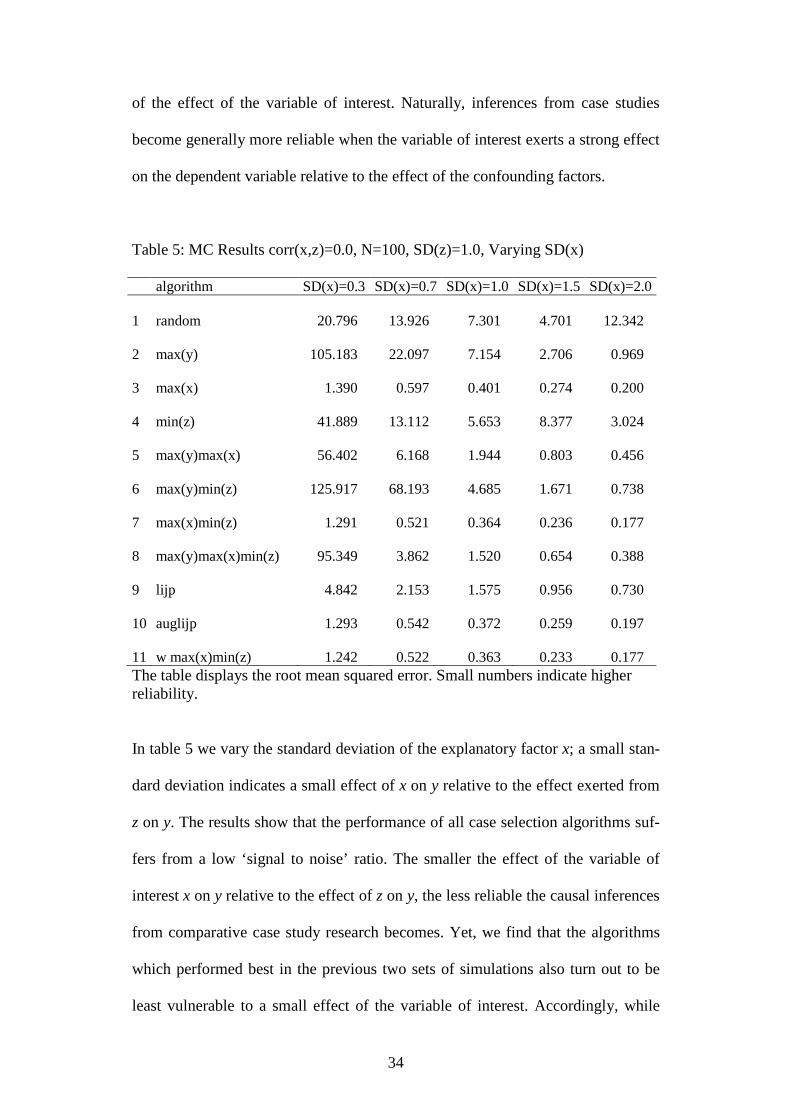
Finally, we examine how algorithms respond to variation in the strength

34

of the effect of the variable of interest. Naturally, inferences from case studies

become generally more reliable when the variable of interest exerts a strong effect

on the dependent variable relative to the effect of the confounding factors.

Table 5: MC Results corr(x,z)=0.0, N=100, SD(z)=1.0, Varying SD(x)

algorithm SD(x)=0.3 SD(x)=0.7 SD(x)=1.0 SD(x)=1.5 SD(x)=2.0

1 random 20.796 13.926 7.301 4.701 12.342

2 max(y) 105.183 22.097 7.154 2.706 0.969

3 max(x) 1.390 0.597 0.401 0.274 0.200

4 min(z) 41.889 13.112 5.653 8.377 3.024

5 max(y)max(x) 56.402 6.168 1.944 0.803 0.456

6 max(y)min(z) 125.917 68.193 4.685 1.671 0.738

7 max(x)min(z) 1.291 0.521 0.364 0.236 0.177

8 max(y)max(x)min(z) 95.349 3.862 1.520 0.654 0.388

9 lijp 4.842 2.153 1.575 0.956 0.730

10 auglijp 1.293 0.542 0.372 0.259 0.197

11 w max(x)min(z) 1.242 0.522 0.363 0.233 0.177

The table displays the root mean squared error. Small numbers indicate higherreliability.

In table 5 we vary the standard deviation of the explanatory factor x; a small stan-

dard deviation indicates a small effect of x on y relative to the effect exerted from

z on y. The results show that the performance of all case selection algorithms suf-

fers from a low ‘signal to noise’ ratio. The smaller the effect of the variable of

interest x on y relative to the effect of z on y, the less reliable the causal inferences

from comparative case study research becomes. Yet, we find that the algorithms

which performed best in the previous two sets of simulations also turn out to be

least vulnerable to a small effect of the variable of interest. Accordingly, while

35

inferences do become more unreliable when the effect of the variable of interest

becomes small relative to the total variation of the dependent variable, compara-

tive case studies are not simply confined to analyzing the main determinant of the

phenomenon of interest if one of the top performing case selection algorithms are

used. As in the previous sets of simulations, we find that little is gained by

employing more complicated functions for aggregating information from more

than one variable as, for example, the ratio (auglijp) or weighting by the variance

of x and z (w max(x)min(z)). Sticking to the most basic aggregation function has

little cost, if any.

Before we conclude from our findings on the optimal choice of case

selection algorithms, we briefly report results from additional Monte Carlo

simulations which we show in full in the appendix to the paper. First, weighting x

and z by their respective sample range becomes more important when the data

generating process includes correlation between x and z and the effect of x on y is

relatively small (see appendix table 1). In this case, weighting both the variation

of x and z before using the max(x)min(z) selection rule for identifying two cases

slightly increases the reliability of causal inferences.

Second, we also conducted the full range of Monte Carlo simulations with

a dichotomous dependent variable (see appendix tables 2 to 5). We find that the

algorithms that perform best with a continuous dependent variable also dominate

with respect to reliability when we analyze dichotomous dependent variables. Yet,

causal inferences from comparative qualitative case study research become far

less reliable when the dependent variable is dichotomous for all selection algo-

rithms compared to the case of a continuous dependent variable. The root mean

squared error roughly doubles for the better performing algorithms. As a conse-

36

quence, causal inferences with a binary dependent variable and an additional

complication (either a non-trivial correlation between x and z or a relatively small

effect of x on y) are not reliable. Accordingly, qualitative researchers should not

throw away variation and analyze continuous or categorical dependent variables

whenever possible. Where the dependent variable is dichotomous, qualitative re-

search is confined to what most qualitative researchers actually do in these situa-

tions: trying to identify strong and deterministic relationships or necessary condi-

tions (Dion 1998; Seawright 2002). In both cases, the strong deterministic effect

of x on y compensates for the low level of information in the data.

Applied qualitative researchers can take away eight lessons from our

Monte Carlo simulations: First, and most fundamentally, the ex ante validity of

generalizations from comparative case studies crucially depends on what we have

dubbed case selection algorithms. Second, ceteris paribus, selecting cases from a

larger sample gives more reliable results. Third, for all the better performing

selection algorithms it holds that ignoring information on the dependent variable

makes inferences much more reliable. Fourth, selecting cases based on the vari-

able of interest and confounding factors improves the reliability of causal infer-

ences in comparison to selection algorithms that consider just the variable of in-

terest or just confounding factors. Fifth, correlation between the variable of inter-

est and confounding factors renders inferences less reliable. Sixth, inferences

about relatively strong effects are more reliable than inferences about relatively

weak effects. Seventh, the reliability of inferences depends on the variation in the

dependent variable scholars can analyze. Accordingly, throwing away information

by dichotomizing the dependent variable is a bad idea. A continuous dependent

variable allows for more valid inferences and a dichotomous dependent variable

37

should only be used if there is no alternative. Eighth, and lastly, employing basic

functions for aggregating information from more than one variable such as

maximizing the difference between variation of x and variation of z does not re-

duce by much the ex ante validity of case selection compared to more complicated

aggregation functions such as maximizing the ratio or the variance-weighted

difference. The only exceptions occur if x and z are highly correlated and the

effect of x on y is relatively small compared to the effect of z on y. As a general

rule, applied researchers will not lose much by opting for the most basic

aggregation function.

7. An Application: Cease-Fire Agreements and the Duration of Peace

To illustrate the implications of our analysis, we now turn to an application of our

case selection algorithms to an existing study.15 Fortna (2004) provides a book-

length study of the effect of cease-fire agreements on the durability of peace

between two belligerent parties, covering the period 1946 to 1997. She uses a

mixture of methods, applying quantitative survival analysis methods to a sample

of 48 cease-fire agreements together with a qualitative survey of these agreements

and a selection of two cases for in-depth study. The cases are the conflicts

between India and Pakistan and between Israel and Syria. Case selection is

justified mainly on the basis that Fortna (2004) regards these as providing a “hard

test of the theory” (page 56), given the “intractable nature of these conflicts”

(page 57).16 In all research designs, she finds that stronger peace agreements tend

to result in longer lasting peace.

15 More often than not, it is hard to find information that allows the replication of results inqualitative research. This not only refers to the information used in the qualitative analysis but alsoto the case selection algorithm.16 Observe that this information does not allow us to replicate the case selection. Thismatters the more as Fortna apparently used none of the 11 algorithms that we study here. We

38

We choose to replicate this study because Fortna makes the dataset on

which her analysis is based publicly available. Other qualitative researchers do not

allow access to their data and also did not respond to our data requests. Equipped

with Fortna’s dataset, we can apply the full set of algorithms to see, firstly, which

cases each algorithm selects and, secondly, compute the ‘causal effects’ based on

this selection.

The dependent variable y is the number of months that peace lasted after

the cease-fire came into existence and the central explanatory variable x is an

index of the strength of this agreement (coded by Fortna and measured by such

requirements as the withdrawal of forces, the introduction of demilitarized zones,

dispute-resolution procedures and outside peacekeeping forces), which runs from

0 to 8 in her “short dataset”. Included control variables measure whether the

armed conflict resulted in a tie rather than a military victory for one of the parties,

the number of battle deaths, the number of past militarized disputes between the

parties to account for conflict history, whether the conflict threatens the sheer

existence of one of the parties, whether the parties are geographically contiguous,

and the relative military capabilities of the belligerents. The purpose of these

control variables is to account for the severity and “intractability” of a conflict.

We use a standardized index of this set of control variables as our z variable.17

Table 6 displays the selected cases and the computed effects for our case

selection algorithms. To start with, note that none of our explicit selection

algorithms selects the two cases selected by Fortna (2004). Selecting on the basis

believe that her case selection is based on an intuitive understanding of cases rather than a strictalgorithm that uses explicit information.17 We also employ indexes based on principal component and factor scores of all control variableswith roughly similar results

39

of a “hard test of the theory” ultimately allows a subjective judgment on which

two cases constitute such a hard test.

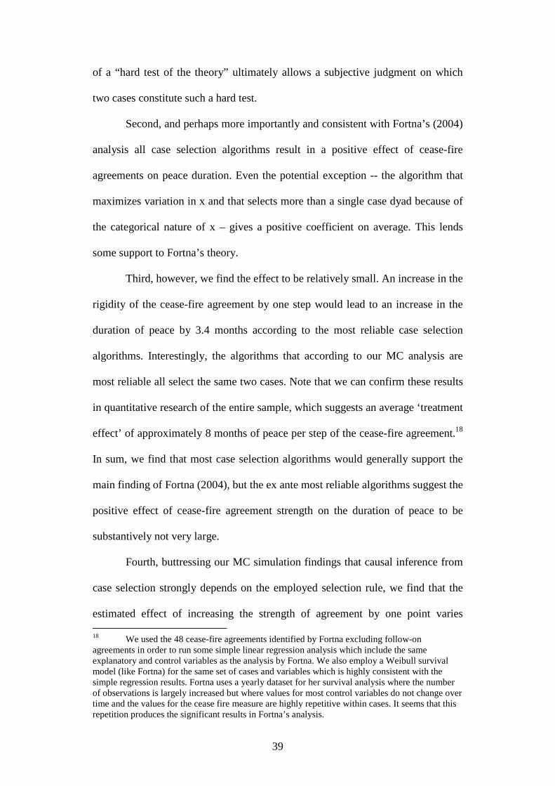
Second, and perhaps more importantly and consistent with Fortna’s (2004)

analysis all case selection algorithms result in a positive effect of cease-fire

agreements on peace duration. Even the potential exception -- the algorithm that

maximizes variation in x and that selects more than a single case dyad because of

the categorical nature of x – gives a positive coefficient on average. This lends

some support to Fortna’s theory.

Third, however, we find the effect to be relatively small. An increase in the

rigidity of the cease-fire agreement by one step would lead to an increase in the

duration of peace by 3.4 months according to the most reliable case selection

algorithms. Interestingly, the algorithms that according to our MC analysis are

most reliable all select the same two cases. Note that we can confirm these results

in quantitative research of the entire sample, which suggests an average ‘treatment

effect’ of approximately 8 months of peace per step of the cease-fire agreement.18

In sum, we find that most case selection algorithms would generally support the

main finding of Fortna (2004), but the ex ante most reliable algorithms suggest the

positive effect of cease-fire agreement strength on the duration of peace to be

substantively not very large.

Fourth, buttressing our MC simulation findings that causal inference from

case selection strongly depends on the employed selection rule, we find that the

estimated effect of increasing the strength of agreement by one point varies

18 We used the 48 cease-fire agreements identified by Fortna excluding follow-onagreements in order to run some simple linear regression analysis which include the sameexplanatory and control variables as the analysis by Fortna. We also employ a Weibull survivalmodel (like Fortna) for the same set of cases and variables which is highly consistent with thesimple regression results. Fortna uses a yearly dataset for her survival analysis where the numberof observations is largely increased but where values for most control variables do not change overtime and the values for the cease fire measure are highly repetitive within cases. It seems that thisrepetition produces the significant results in Fortna’s analysis.

40

largely and reaches a maximum of an increase of almost 209 months. This result,

however, is based on the application of an unreliable case selection algorithm.

Specifically, large effects depend on selection on the dependent variable – a

procedure that is likely to give biased results as King, Keohane and Verba assure

readers (PAGE????) and our MC analysis demonstrates.

41

Table 6. Case selection and effect strength in an application to Fortna (2004).

Algorithm

1 Random Selected Pair US-North Korea 1952 / Israel-Syria 1982effect +63.5

2max(y) Selected Pair

Korea (US-China, US-North Korea,South Korea-China, South Korea-NorthKorea) 1952 / Turkey-Cyprus July 1974

effect +208.86

3

max(x) Selected Pairs

Russo-Hungarian/Vietnamese;Vietnamese/Yom-Kippur,

Ugandan/Tanzanian, Falklands,Sino/Vietnamese

effect -24.32 … +42.1

4 min(z) Selected PairPalestine (Israel-Iraq) 1948 / Football (El

Salvador-Honduras) 1969effect +108.8

5max(y)max(x) Selected Pair

Korea (US-China, US-North Korea,South Korea-China, South Korea-NorthKorea) 1952 / Azerbaijan-Armenia 1992

effect +92.8

6 max(y)min(z) Selected PairKorean(US-China) 1952 / Turkey-

Cyprus 1974effect +208.86

7 max(x)min(z) Selected PairVietnam-USA 1973 / Vietnam-Republic

of Vietnam 1975effect +3.4

8 max(y)max(x)min(z) Selected PairKorea (South Korea-North Korea) 1952 /

Azerbaijan-Armenia 1992effect +92.8

9 Lijp Selected PairPalestine (Israel-Iraq) 1948 / Football (El

Salvador-Honduras) 1969effect +108.8

10 Auglijp Selected PairVietnam-USA 1973 / Vietnam-Republic

of Vietnam 1975effect +3.4

11 w max(x)min(z) Selected PairVietnam-USA 1973 / Vietnam-Republic

of Vietnam 1975effect +3.4

8. Conclusion

Qualitative research can be used for much more than making causal inferences.

But when researchers aim at generalizing their findings, getting the selection of

42

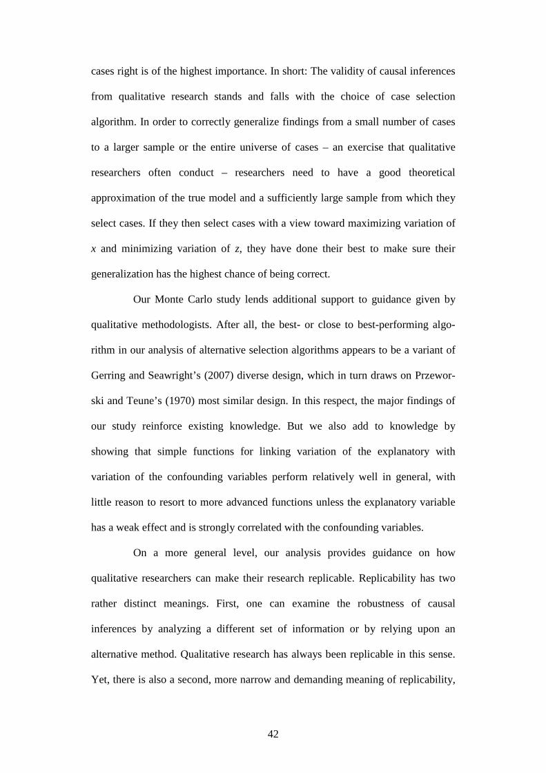
cases right is of the highest importance. In short: The validity of causal inferences

from qualitative research stands and falls with the choice of case selection

algorithm. In order to correctly generalize findings from a small number of cases

to a larger sample or the entire universe of cases – an exercise that qualitative

researchers often conduct – researchers need to have a good theoretical

approximation of the true model and a sufficiently large sample from which they

select cases. If they then select cases with a view toward maximizing variation of

x and minimizing variation of z, they have done their best to make sure their

generalization has the highest chance of being correct.

Our Monte Carlo study lends additional support to guidance given by

qualitative methodologists. After all, the best- or close to best-performing algo-

rithm in our analysis of alternative selection algorithms appears to be a variant of

Gerring and Seawright’s (2007) diverse design, which in turn draws on Przewor-

ski and Teune’s (1970) most similar design. In this respect, the major findings of

our study reinforce existing knowledge. But we also add to knowledge by

showing that simple functions for linking variation of the explanatory with

variation of the confounding variables perform relatively well in general, with

little reason to resort to more advanced functions unless the explanatory variable

has a weak effect and is strongly correlated with the confounding variables.

On a more general level, our analysis provides guidance on how

qualitative researchers can make their research replicable. Replicability has two

rather distinct meanings. First, one can examine the robustness of causal

inferences by analyzing a different set of information or by relying upon an

alternative method. Qualitative research has always been replicable in this sense.

Yet, there is also a second, more narrow and demanding meaning of replicability,

43

which requires that by using the same information and the same methods one

should arrive at the same results. If an analysis cannot be thus replicated, one

should seriously doubt the inferences from that study. Our study suggests that

researchers need to provide three pieces of information to make a comparative

case study replicable in this sense: the provision of sufficient information on the

sample from which they select cases, a comprehensive description of the set of

variables they use to select cases, and a precise statement of the case selection

algorithm employed. Given these pieces of information, qualitative research is in

principle as replicable as quantitative analyses. Even more importantly, this

information gives other scholars sufficient clues about the ex ante external

validity of the findings derived from comparative case study research.

References

Bartels, Larry M. 2004, The Unfulfilled Promises of Quantitative Imperialism, inHenry Brady and David Collier (eds.): Rethinking Social Inquiry: DiverseTools, Shared Standards, Rowman and Littlefield, Lanham, 69-83.

Brady, Henry E. 2002, Models of Causal Inference: Going Beyond the Neyman–Rubin–Holland Theory, unp. manuscript, Midwest Political ScienceAssociation, Chicago, IL, .

Brady, Henry E. 2004, Doing good and doing better: How far does the Quantita-tive Template get us? in: Henry Brady and David Collier (eds.): Rethink-ing Social Inquiry: Diverse Tools, Shared Standards, Rowman and Little-field, Lanham, 53-83.

Brady, Henry E. 2008, Causation and Explanation in Social Science. in: Janet M.Box-Steffensmeier, Henry E. Brady, and David Collier (editors): OxfordHandbook of Political Methodology, Oxford University Press, Oxford,217-270.

Brady, Henry E., David Collier and Jason Seawright 2006, Toward a PluralisticVision of Methodology, Political Analysis 14, 353-368.

Braumoeller, Bear F. and Gary Goertz 2000, The Methodology of NecessaryConditions. American Journal of Political Science 44, 844-858.

Braumoeller, Bear F. 2003, Causal Complexity and the Study of Politics, PoliticalAnalysis 11, 209-233.

Collier, David 1993, The Comparative Method, in: Ada W. Finifter (ed), Political

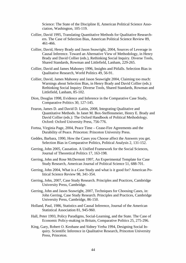
44

Science: The State of the Discipline II, American Political Science Asso-ciation, Washington, 105-119.

Collier, David 1995, Translating Quantitative Methods for Qualitative Research-ers. The Case of Selection Bias, American Political Science Review 89,461-466.

Collier, David, Henry Brady and Jason Seawright, 2004, Sources of Leverage inCausal Inference. Toward an Alternative View of Methodology, in HenryBrady and David Collier (eds.), Rethinking Social Inquiry. Diverse Tools,Shared Standards, Rowman and Littlefield, Lanham, 229-265.

Collier, David and James Mahoney 1996, Insights and Pitfalls. Selection Bias inQualitative Research, World Politics 49, 56-91.

Collier, David, James Mahoney and Jason Seawright 2004, Claiming too much:Warnings about Selection Bias, in Henry Brady and David Collier (eds.):Rethinking Social Inquiry: Diverse Tools, Shared Standards, Rowman andLittlefield, Lanham, 85-102.

Dion, Douglas 1998, Evidence and Inference in the Comparative Case Study,Comparative Politics 30, 127-145.

Fearon, James D. and David D. Laitin, 2008, Integrating Qualitative andQuantitative Methods. In Janet M. Box-Steffensmeier, Henry E. Brady andDavid Collier (eds.): The Oxford Handbook of Political Methodology.Oxford: Oxford University Press, 756-776.

Fortna, Virginia Page, 2004, Peace Time – Cease-Fire Agreements and theDurability of Peace. Princeton: Princeton University Press.

Geddes, Barbara, 1990, How the Cases you Choose affect the Answers you get.Selection Bias in Comparative Politics, Political Analysis 2, 131-152.

Gerring, John 2005, Causation. A Unified Framework for the Social Sciences,Journal of Theoretical Politics 17, 163-198.

Gerring, John and Rose McDermott 1997, An Experimental Template for CaseStudy Research, American Journal of Political Science 51, 688-701.

Gerring, John 2004, What is a Case Study and what is it good for? American Po-litical Science Review 98, 341-354.

Gerring, John, 2007, Case Study Research. Principles and Practices, CambridgeUniversity Press, Cambridge.

Gerring, John and Jason Seawright, 2007, Techniques for Choosing Cases, in:John Gerring, Case Study Research. Principles and Practices, CambridgeUniversity Press, Cambridge, 86-150.

Holland, Paul, 1986, Statistics and Causal Inference, Journal of the AmericanStatistical Association 81, 945-960.

Hall, Peter 1993, Policy Paradigms, Social-Learning, and the State. The Case ofEconomic Policy-making in Britain, Comparative Politics 25, 275-296.

King, Gary, Robert O. Keohane and Sidney Verba 1994, Designing Social In-quiry. Scientific Inference in Qualitative Research, Princeton UniversityPress, Princeton.

45

Lijphart, Arend 1971, Comparative Politics and the Comparative Method, Ameri-can Political Science Review 65, 682- 693.

Lijphart, Arend 1975, Comparable Cases Strategy in Comparative Research,Comparative Political Studies 8, 158-177.

Mahoney, James 2007, Qualitative Methodology and Comparative Politics. Com-parative Political Studies 40, 122-144.

Mahoney, James and Gary Goertz 2006, A Tale of Two Cultures. ContrastingQuantitative and Qualitative Research, Political Analysis 14, 227-249.

McKeown, Timothy 2004, Case Studies and the Limits of the QuantitativeWorldview, in Henry Brady and David Collier (eds.): Rethinking SocialInquiry: Diverse Tools, Shared Standards, Rowman and Littlefield,Lanham, 139-167.

Meckstroth, Theodore 1975, “Most Different Systems” and “Most Similar Sys-tems”: A Study in the Logic of Comparative Inquiry. Comparative Politi-cal Studies 8, 133-177.

Ostrom, Elinor 1990, Governing the Commons. The Evolution of Institutions forCollective Action, Cambridge University Press, Cambridge.

Pearl 2009.

Przeworski, Adam and Henry Teune 1970, The Logic of Comparative Social In-quiry. New York: Wiley.

Seawright, Jason 2002, Testing for Necessary and/or Sufficient Causation: WhichCases are Relevant? Political Analysis 10, 178-193.

Seawright, Jason and John Gerring 2008, Case Selection Techniques in CaseStudy Research: A Menu of Qualitative and Quantitative Options, PoliticalResearch Quarterly 61, 294-308.

Sekhon, Jasjeet S. 2004, Quality Meets Quantity: Case Studies, Conditional Prob-ability, and Counterfactuals. Perspectives on Politics 2, 281-293.

Tarrow, Sidney, 2010, The Strategy of Paired Comparisons. Toward A Theory ofPractice, Comparative Political Studies 43, 230-259.

46

Appendix Table 1: MC Results Continuous Outcome SD(x)=0.3, N=100, SD(z)=1.0, Varying Correlation (x,z)

algorithm criterion corr=-0.9 corr=-0.7 corr=-0.3 corr=0 corr=0.3 corr=0.7 corr=0.9

1 random rmse 20.411 26.946 25.505 20.796 43.789 49.871 31.853p≤0 0.615 0.571 0.492 0.421 0.418 0.323 0.266

2 max(y) rmse 57.993 99.264 270.517 105.183 136.001 21.068 16.749p≤0 0.913 0.822 0.525 0.266 0.098 0.013 0.004

3 max(x) rmse 3.021 2.402 1.572 1.390 1.610 2.524 2.908p≤0 0.910 0.802 0.483 0.276 0.111 0.029 0.006

4 min(z) rmse 69.408 27.372 32.238 41.889 20.927 373.118 68.821p≤0 0.482 0.460 0.425 0.430 0.453 0.441 0.459

5 max(y)max(x) rmse 21.081 49.380 83.554 56.402 32.309 13.379 11.375p≤0 0.943 0.845 0.514 0.245 0.073 0.008 0.002

6 max(y)min(z) rmse 342.961 2005.662 105.559 125.917 197.299 86.462 99.143p≤0 0.603 0.451 0.337 0.236 0.183 0.137 0.105

7 max(x)min(z) rmse 3.015 1.862 1.380 1.291 1.343 1.819 3.100p≤0 0.402 0.331 0.261 0.281 0.289 0.343 0.368

8 max(y)max(x)min(z) rmse 146.883 80.848 43.529 95.349 122.412 35.729 40.032p≤0 0.656 0.466 0.286 0.205 0.151 0.092 0.052

9 lijp rmse 11.206 7.000 4.714 4.842 5.319 7.246 11.404p≤0 0.469 0.433 0.387 0.411 0.403 0.437 0.442

10 auglijp rmse 2.773 1.871 1.377 1.293 1.340 1.800 2.851p≤0 0.399 0.333 0.261 0.286 0.286 0.336 0.357

11 w max(x)min(z) rmse 2.319 1.668 1.277 1.242 1.207 1.611 2.350p≤0 0.446 0.353 0.281 0.257 0.242 0.265 0.245

12 w max(y)max(x)min(z) rmse 16.091 9.189 4.952 4.510 4.768 6.722 9.629p≤0 0.676 0.391 0.179 0.116 0.095 0.065 0.020

47

Appendix Table 2: MC Results Binary Outcome SD(x)=1.0, SD(z)=1.0, corr(x,z)=0, Varying Sample Size N

algorithm criterion N=20 N=40 N=60 N=80 N=100

1 random rmse 3.625 2.637 1.906 2.927 1.638p≤0 0.618 0.642 0.646 0.648 0.638

2 max(y) rmse 3.044 3.130 3.361 10.140 7.093p≤0 0.257 0.241 0.262 0.296 0.276

3 max(x) rmse 0.818 0.825 0.829 0.836 0.831p≤0 0.297 0.234 0.200 0.204 0.161

4 min(z) rmse 3.039 1.745 6.143 4.306 2.881p≤0 0.656 0.662 0.694 0.638 0.632

5 max(y)max(x) rmse 0.767 0.785 0.794 0.804 0.803p≤0 0.084 0.051 0.035 0.034 0.016

6 max(y)min(z) rmse 3.914 3.184 7.053 5.224 5.022p≤0 0.253 0.261 0.243 0.236 0.237

7 max(x)min(z) rmse 0.813 0.805 0.823 0.824 0.826p≤0 0.334 0.217 0.228 0.196 0.174

8 max(y)max(x)min(z) rmse 0.732 0.756 0.778 0.783 0.787p≤0 0.066 0.026 0.029 0.017 0.006

9 lijp rmse 0.927 0.945 0.909 0.908 0.911p≤0 0.576 0.573 0.590 0.564 0.533

10 auglijp rmse 0.811 0.803 0.819 0.823 0.819p≤0 0.365 0.259 0.263 0.242 0.205

11 w max(x)min(z) rmse 0.812 0.807 0.823 0.823 0.825p≤0 0.334 0.221 0.228 0.193 0.172

12 w max(y)max(x)min(z) rmse 0.732 0.755 0.780 0.784 0.787p≤0 0.064 0.023 0.033 0.019 0.006

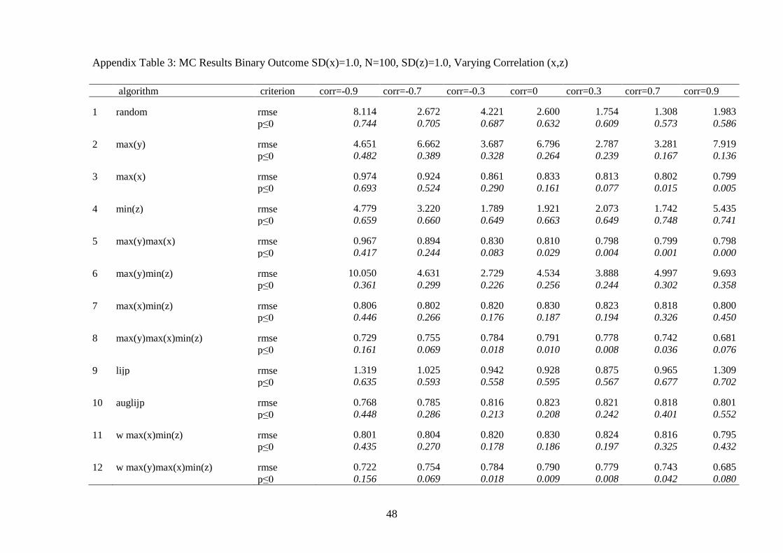
48

Appendix Table 3: MC Results Binary Outcome SD(x)=1.0, N=100, SD(z)=1.0, Varying Correlation (x,z)

algorithm criterion corr=-0.9 corr=-0.7 corr=-0.3 corr=0 corr=0.3 corr=0.7 corr=0.9

1 random rmse 8.114 2.672 4.221 2.600 1.754 1.308 1.983p≤0 0.744 0.705 0.687 0.632 0.609 0.573 0.586

2 max(y) rmse 4.651 6.662 3.687 6.796 2.787 3.281 7.919p≤0 0.482 0.389 0.328 0.264 0.239 0.167 0.136

3 max(x) rmse 0.974 0.924 0.861 0.833 0.813 0.802 0.799p≤0 0.693 0.524 0.290 0.161 0.077 0.015 0.005

4 min(z) rmse 4.779 3.220 1.789 1.921 2.073 1.742 5.435p≤0 0.659 0.660 0.649 0.663 0.649 0.748 0.741

5 max(y)max(x) rmse 0.967 0.894 0.830 0.810 0.798 0.799 0.798p≤0 0.417 0.244 0.083 0.029 0.004 0.001 0.000

6 max(y)min(z) rmse 10.050 4.631 2.729 4.534 3.888 4.997 9.693p≤0 0.361 0.299 0.226 0.256 0.244 0.302 0.358

7 max(x)min(z) rmse 0.806 0.802 0.820 0.830 0.823 0.818 0.800p≤0 0.446 0.266 0.176 0.187 0.194 0.326 0.450

8 max(y)max(x)min(z) rmse 0.729 0.755 0.784 0.791 0.778 0.742 0.681p≤0 0.161 0.069 0.018 0.010 0.008 0.036 0.076

9 lijp rmse 1.319 1.025 0.942 0.928 0.875 0.965 1.309p≤0 0.635 0.593 0.558 0.595 0.567 0.677 0.702

10 auglijp rmse 0.768 0.785 0.816 0.823 0.821 0.818 0.801p≤0 0.448 0.286 0.213 0.208 0.242 0.401 0.552

11 w max(x)min(z) rmse 0.801 0.804 0.820 0.830 0.824 0.816 0.795p≤0 0.435 0.270 0.178 0.186 0.197 0.325 0.432

12 w max(y)max(x)min(z) rmse 0.722 0.754 0.784 0.790 0.779 0.743 0.685p≤0 0.156 0.069 0.018 0.009 0.008 0.042 0.080

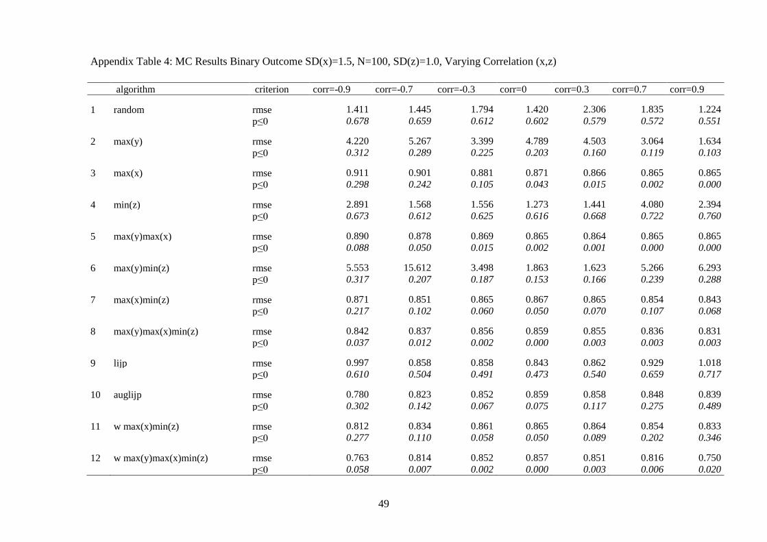
49

Appendix Table 4: MC Results Binary Outcome SD(x)=1.5, N=100, SD(z)=1.0, Varying Correlation (x,z)

algorithm criterion corr=-0.9 corr=-0.7 corr=-0.3 corr=0 corr=0.3 corr=0.7 corr=0.9

1 random rmse 1.411 1.445 1.794 1.420 2.306 1.835 1.224p≤0 0.678 0.659 0.612 0.602 0.579 0.572 0.551

2 max(y) rmse 4.220 5.267 3.399 4.789 4.503 3.064 1.634p≤0 0.312 0.289 0.225 0.203 0.160 0.119 0.103

3 max(x) rmse 0.911 0.901 0.881 0.871 0.866 0.865 0.865p≤0 0.298 0.242 0.105 0.043 0.015 0.002 0.000

4 min(z) rmse 2.891 1.568 1.556 1.273 1.441 4.080 2.394p≤0 0.673 0.612 0.625 0.616 0.668 0.722 0.760

5 max(y)max(x) rmse 0.890 0.878 0.869 0.865 0.864 0.865 0.865p≤0 0.088 0.050 0.015 0.002 0.001 0.000 0.000

6 max(y)min(z) rmse 5.553 15.612 3.498 1.863 1.623 5.266 6.293p≤0 0.317 0.207 0.187 0.153 0.166 0.239 0.288

7 max(x)min(z) rmse 0.871 0.851 0.865 0.867 0.865 0.854 0.843p≤0 0.217 0.102 0.060 0.050 0.070 0.107 0.068

8 max(y)max(x)min(z) rmse 0.842 0.837 0.856 0.859 0.855 0.836 0.831p≤0 0.037 0.012 0.002 0.000 0.003 0.003 0.003

9 lijp rmse 0.997 0.858 0.858 0.843 0.862 0.929 1.018p≤0 0.610 0.504 0.491 0.473 0.540 0.659 0.717

10 auglijp rmse 0.780 0.823 0.852 0.859 0.858 0.848 0.839p≤0 0.302 0.142 0.067 0.075 0.117 0.275 0.489

11 w max(x)min(z) rmse 0.812 0.834 0.861 0.865 0.864 0.854 0.833p≤0 0.277 0.110 0.058 0.050 0.089 0.202 0.346

12 w max(y)max(x)min(z) rmse 0.763 0.814 0.852 0.857 0.851 0.816 0.750p≤0 0.058 0.007 0.002 0.000 0.003 0.006 0.020

50

Appendix Table 5: MC Results Binary Outcome SD(x)=0.3, N=100, SD(z)=1.0, Varying Correlation (x,z)

algorithm criterion corr=-0.9 corr=-0.7 corr=-0.3 corr=0 corr=0.3 corr=0.7 corr=0.9

1 random rmse 8.995 8.163 80.732 6.335 7.917 12.190 11.440p≤0 0.822 0.805 0.741 0.721 0.682 0.641 0.613

2 max(y) rmse 106.287 11.848 19.486 20.691 17.370 10.001 8.574p≤0 0.688 0.611 0.479 0.427 0.334 0.291 0.233

3 max(x) rmse 1.446 1.297 0.992 0.776 0.589 0.412 0.383p≤0 0.979 0.933 0.737 0.546 0.345 0.116 0.075

4 min(z) rmse 131.176 12.420 5.636 9.436 6.493 6.991 9.614p≤0 0.733 0.714 0.705 0.739 0.742 0.766 0.775

5 max(y)max(x) rmse 1.554 1.393 1.003 0.692 0.469 0.348 0.340p≤0 0.912 0.791 0.500 0.273 0.108 0.018 0.010

6 max(y)min(z) rmse 148.288 21.529 16.576 15.011 11.756 17.360 23.556p≤0 0.466 0.446 0.424 0.404 0.410 0.451 0.439

7 max(x)min(z) rmse 1.233 0.838 0.777 0.766 0.793 0.838 1.202p≤0 0.713 0.660 0.591 0.593 0.618 0.670 0.730

8 max(y)max(x)min(z) rmse 1.677 0.790 0.659 0.569 0.632 0.763 1.690p≤0 0.376 0.311 0.281 0.222 0.261 0.290 0.372

9 lijp rmse 4.187 2.538 1.642 1.772 2.002 2.222 3.240p≤0 0.726 0.710 0.689 0.729 0.722 0.755 0.757

10 auglijp rmse 1.199 0.829 0.778 0.764 0.790 0.827 1.106p≤0 0.718 0.657 0.597 0.594 0.619 0.666 0.716

11 w max(x)min(z) rmse 1.129 0.825 0.792 0.769 0.753 0.723 0.876p≤0 0.751 0.657 0.610 0.578 0.578 0.598 0.619

12 w max(y)max(x)min(z) rmse 1.330 0.779 0.689 0.586 0.622 0.590 0.873p≤0 0.476 0.359 0.296 0.217 0.241 0.239 0.244