Case Selection and Causal Inference in Qualitative Research · Case Selection and Causal Inference in Qualitative Research Thomas Plümpera, Vera E. Troegerb, and Eric Neumayerc a

Case Selection and Causal Inference in Qualitative Research Thomas Plümpera, Vera E. Troegerb, and Eric Neumayerc

a Department of Government, University of Essex, Wivenhoe Park, Colchester

CO4 3SQ, UK b Department of Economics and PaIS, University of Warwick,

[email protected] c Department of Geography and Environment, London School of Economics

and Political Science (LSE), London WC2A 2AE, UK, [email protected] Corresponding author: Thomas Plümper.

1

Case Selection and Causal Inference in Qualitative Research

Abstract

The validity of causal inferences in qualitative research depends on the selection

of cases. We contribute to current debates on qualitative research designs by using

Monte Carlo techniques to evaluate the performance of different case selection

techniques or algorithms. We show that causal inference from qualitative research

becomes more reliable when researchers select cases from a larger sample,

maximize the variation in the variable of interest, simultaneously minimize

variation of the confounding factors, and ignore all information on the dependent

variable. We also demonstrate that causal inferences from qualitative research

become much less reliable when the variable of interest is strongly correlated with

confounding factors, the effect of the variable of interest becomes small relative to

the effect of the confounding factors, and when researchers analyze dichotomous

dependent variables.

2

1. Introduction

Causal inferences may neither be the comparative advantage of qualitative re-

search nor the main reason for comparing cases. However, applied qualitative

researchers often formulate causal inferences and generalize their findings derived

from the study of comparative cases.1 Many such studies have been published

with leading publishers and in leading journals and their findings rank

prominently among the most influential work in the social sciences. To give but

two examples: Elinor Ostrom’s Nobel Prize-awarded study of solutions to

common pool problems suggests eight “situational variables” shaping the

probability of successful and stable local resource management (Ostrom 1990:

88ff.). Ostrom formulates these findings as necessary conditions determining the

ability of actors to overcome commons problems. Similarly, after a careful

examination of economic policy decisions in Great Britain over the 1970s and

1980s, Peter Hall (1993: 287-292) concludes by formulating broad generalizations

about the process of social learning and the influence of paradigmatic ideas on

policy-making and change. Qualitative methodologists agree that comparative

case study research should aim and does aim at generalizations and causal

inference (Collier, Brady and Seawright 2004; Mahoney and Goertz 2006).2 They

also agree that if qualitative researchers are interested in making causal

1 The falsification of a deterministic theory by a single deviant case shows that not all

causal inferences depend on generalizations.

2 This does not imply that nothing can be learned from inductive research (McKeown

2004). Perhaps most importantly, Gerring and Seawright (2007: 149) correctly state that

selection algorithms for testing theories differ from algorithms that aim at theory

development.

3

inferences, the selection of cases must be based on a reasonable selection rule3

and on knowledge of the universe of cases or a reasonably large sample (Gerring

and Seawright 2007: 90).

This paper contributes to recent developments in qualitative research

methodology. Using Monte Carlo (MC) experiments, which itself is a novelty to

qualitative methodology, we show that causal inferences become ex ante more

valid when scholars select cases from a larger sample, when they analyze

relatively important determinants of the phenomenon of interest, and when they

use an optimal case selection algorithm. We analyze the performance of twelve

case selection algorithms to demonstrate on which information case selection

ought to rely and, conversely, which information ought to be ignored. The MC

analyses reveal that some algorithms greatly outperform others. Our experiments

second qualitative methodologists and statistical theory that selection algorithms

that use sample information on both the independent variable of interest (or

treatment or operative variable) and the potentially confounding control variables

perform significantly better than other algorithms. Thus, in respect to the optimal

selection algorithm our results lend, perhaps unsurprisingly, support to a fairly

common practice in comparative case study research: simultaneous sampling on

the variable of interest (x) and on confounding factors (z). Yet, researchers can

still choose between numerous algorithms which all select on both x and z. This

paper is the first to demonstrate that a fairly simple algorithm of combining

information on x and z, namely an algorithm that maximizes the unweighted

difference of the distances in x and z, outperforms alternative, more complicated

3 We prefer to call these rules case selection ‘algorithm’ to emphasize the non-arbitrary

way in which cases ought to be selected.

4

algorithms that use, for example, the ratio of x and z (as suggested by Lijphart as

early as 1975) or mathematically slightly more sophisticated variants which

weight x and z by their respective standard deviation.

In addition, algorithms that exclusively or partly use information on the

dependent variable perform far worse than algorithms that refrain from doing so.

On average, the worst performing algorithm, which selects on the dependent

variable with no regard to variation of the variable of interest or of the control

variable, is roughly 50 times less reliable than the best performing algorithms.

Thus, choosing the right way to select cases matters – and it matters a lot. Case

selection stands at the core of improving the validity of causal inferences from

qualitative research.4 By using an optimal case selection algorithm, qualitative

researchers can improve their causal inferences.

We wish to be clear about what we do not do in this paper. First, we do

not compare the validity of inferences based on qualitative research to inferences

drawn from quantitative research. In principle, MC analyses could be used to do

exactly this, but a fair comparison would require more complex data generating

processes than the one we use here. Second, we refrain from analyzing case selec-

tion algorithms for qualitative research with more than two cases. Note, however,

that all major results we show here carry over. Third, we also say nothing about

causal inferences from designs that use a single case to study theoretical claims of

necessity or sufficiency (Braumoeller and Goertz 2000; Seawright 2002). Fourth,

we do not explore algorithms of case selection when researchers are interested in 4 Note, we do not say that qualitative researchers just need to select two cases which both

lie on the regression line of a perfectly specified model estimated using the entire

population. Naturally, inference from such two cases would be perfectly valid, but the

advice falls short of being useful as researchers do not know the true model and if they

did, further research would be redundant as it could not infer anything not known already.

5

more than one independent variable. The second and third self-imposed

limitations are closely related to each other because researchers need to analyze

between 1+2·k and 2k cases (depending on the complexity of the theory) when

they are interested in k different exogenous variables. Again, MC analyses are in

principle suited for these questions and we will address them in future work. Fifth

and finally, being solely interested in improving the validity of causal inferences,

we do not consider descriptive inferences or inductive variants of qualitative

research aimed at theory building, the discovery of missing variables, refining the

population of relevant cases, or the like.

2. Algorithms for Case Selection in Qualitative Research

Methodological advice on the selection of cases in qualitative research stands in a

long tradition. John Stuart Mill in his A System of Logic, first published in 1843,

proposed five methods that were meant to enable researchers to make causal

inferences: the method of agreement, the method of difference, the double method

of agreement and difference, the method of residues, and the method of

concomitant variation. Modern methodologists have questioned and criticized the

usefulness and general applicability of Mill’s methods (see, for example, Sekhon

2004). However, without doubt Mill’s proposals had a major and lasting impact

on the development of the two most prominent modern methods, namely the

‘most similar’ and ‘most different’ comparative case study designs (Przeworski

and Teune 1970; Lijphart 1971, 1975; Meckstroth 1975).

Modern comparative case study research usually refers to

Przeworski and Teune’s (1970) discussion of ‘most similar’ and ‘most different’

designs. Yet, it often remains unclear how closely applied researchers follow

6

Przeworski and Teune’s advice. For example, their ‘most similar design’ asks

applied researchers to identify the most similar cases and then explain the

variation in the outcome by variation in relevant variables. Apparently,

Przeworski and Teune believe that factors common to the cases “are irrelevant in

determining the behavior being explained” while “any set of variables that

differentiates (…) corresponding to the observed differences in behavior (…) can

be considered as explaining these patterns of behavior.” (Przeworski and Teune

1970: 34) Unfortunately, both inferences can easily be wrong. A variable that

does not vary in a small sample can have substantive effects in the population.

Similarly, a variable that varies between selected cases does not need to exert a

causal effect. Przeworski and Teune’s (1970: 34) ‘most different design’ also does

not seem to motivate most applied qualitative research. Rather, their most

different design resembles what researchers nowadays call a multilevel design.

Thus, as Seawright and Gerring (2008: 295) point out, these and other

methods of case selection are ‘poorly understood and often misapplied’.

Qualitative researchers often mean very different things when they invoke the

same terms ‘most similar’ or ‘most different’ and usually the description of their

research design is too imprecise to allow readers to assess how exactly cases have

been chosen.

Seawright and Gerring (2008) have therefore provided a formal definition

and classification of these and other techniques of case selection. They suggest

that “in its purest form” (Seawright and Gerring 2008: 304) the ‘most similar’

design chooses cases which appear to be identical on all controls (z) but different

in the variable of interest (x).

7

Similarly, Lijphart (1975: 163) pioneered a formal operationalization of a

variant of this method when he proposed that researchers should maximize “the

ratio between the variance of the operative variables and the variance of the

control variables”. Naturally, the ‘most similar’ technique is not easily applied as

researchers find it difficult to match cases such that they are identical on all

control variables. As Seawright and Gerring (2008: 305) concede: “Unfortunately,

in most observational studies, the matching procedure described previously –

known as exact matching – is impossible.” This impossibility has two sources:

first, researchers usually do not know the true model. Therefore they simply

cannot match on all control variables. And second, even if known to affect the

dependent variable, many variables remain unobserved.

The difficulties that the ‘most similar’ technique encounters have not

prevented qualitative researchers from giving it strong preference over the ‘most

different’ technique. Seawright and Gerring (2008: 306) believe that this

dominance of ‘most similar’ over ‘most different’ is well justified. Defining the

‘most different’ technique as choosing two cases that are identical in the outcome

y and the main variable of interest x but different in all control variables z,5 they

argue that this technique does not generate much leverage. They criticize three

points: first, the chosen cases never represent the entire population (if x can in fact

vary in the population). Second, the lack of variation in x renders it impossible to

5 Gerring (2004: 352) formulates explicitly: “There is little point in pursuing crossunit

analysis if the units in question do not exhibit variation on the dimensions of theoretical

interest and/or the researcher cannot manage to hold other, potentially confounding,

factors constant.”

8

identify causal effects. And third, elimination of rival hypotheses is impossible.6

We add that the absence of variation in the control variables does not imply that

specific control variables have no influence on the outcome – it may well be that

the aggregate influences of all confounding factors cancel each other out. Thus,

the design cannot guarantee valid inferences and the generalization to other

subsamples appears to be beyond the control of the selection process. Seawright

and Gerring also identify a third technique for selecting cases in comparative case

studies, which they label the ‘diverse’ technique. It selects cases so as to

“represent the full range of values characterizing X, Y, or some particular X/Y

relationship” (Seawright and Gerring 2008: 300).7

Perhaps surprisingly, King, Keohane and Verba’s (1994) important

contribution to qualitative research methodology discusses case selection only

from the perspective of unit homogeneity – broadly understood as constant effect

6 The latter criticism appears somewhat unfair since no method can rule out the possibility

of unobserved confounding factors entirely. Of course, well designed experiments get

closest to ruling out this possibility.

7 In addition, Seawright and Gerring (2008) and Gerring and Seawright (2007: 89) discuss

six algorithms that allow making inferences by comparison to a theoretical prior. For

example, the analysis of ‘outliers’ requires the comparison to a case which is an ‘onlier’

(Gerring and Seawright’s terminology). The distinction that the authors draw between

comparative case studies and single case studies has nowadays been generally accepted.

Tarrow (2010: 244) compares the logic of comparative case studies (but explicitly not

single case studies) to the logic of experiments: “Paired comparison is distinct from

single-case studies in several ways. Its distinctiveness can be understood through an

analogy with experimental design. It is similar to experimentation in its ability to compare

the impact of a single variable or mechanism on outcomes of interest. Of course, an

experimenter has the ability to randomly assign subjects to treatment and control groups

(…). All the pairing comparativist can do this respect is to attempt to carefully match the

confounding variables that he or she knows about (but not ones that do not come to

mind).”

9

assumption (King et al. 1994: 92)8 – and selection bias – defined as non-random

selection of cases which are not statistically representative of the population

(Collier 1995: 462).

Selecting cases in a way that does not avoid selection bias negatively

affects the generalizability of inferences. Random sampling from the population

of cases would clearly avoid selection bias. Thus, given the prominence of

selection bias in King et al.’s discussion of case selection, the absence of random

sampling in comparative research seems surprising. But it is not. Random

selection of cases leads to inferences which are correct on average when the

number of case studies approaches infinity, but the sampling deviation is

extremely large. As a consequence, the reliability of single studies of randomly

sampled cases remains low.

The advice King and his co-authors give on case selection, then, lends

additional credibility to common practices chosen by applied qualitative

researchers, namely to avoid truncation of the dependent variable (p. 130, see also

Collier et al. 2004: 91), to avoid selection on the dependent variable (p. 134, see

also Collier et al. 2004: 88), while at the same time selecting according to the

categories of the ‘key causal explanatory variable’.9

8 This interpretation deviates from Holland’s definition of unit homogeneity, which

requires that the conditional effect and the marginal effect are identical, implying that the

size of the independent variable is the same (Holland 1986: 947). To satisfy King et al.’s

definition of unit homogeneity, only the marginal effect has to be identical (King et al.

92-93).

9 King et al. (1994) also repeatedly claim that increasing the number of observations makes

causal inferences more reliable. Qualitative researchers have argued that this view, while

correct in principle, does not do justice to qualitative research (Brady 2004, Bartels 2004,

McKeown 2004). More importantly, they also suggest that the extent to which the logic

of quantitative research can be superimposed on qualitative research designs has limits.

10

Our MC experiments attempt to be as comprehensive as possible

without including algorithms that appear inferior at first sight. We will therefore

cover the techniques (algorithms as we prefer to call them to highlight the

deterministic character of case selection) commonly used in applied research, but

also various permutations and extensions. Assume without much10 loss of

generality a data generating process in which the dependent variable y is a linear

function of a variable of interest x and a control variable z. Ignoring for the time

being standard advice against sampling on the dependent variable, researchers

might wish to maximize variation of y, maximize variation of x, minimize

variation of z or some combination thereof. This leads to seven permutations of

information to choose from, which together with random sampling results in eight

simple case selection algorithms – see table 1.

10 Since we can interpret z as a vector of k control variables, we can generalize findings to

analyses with multiple controls. However, we cannot generalize to selection algorithms

that select two cases on one dimension and two other cases on another dimension of

controls. We leave these issues to future research.

11

Table 1: Simple Case Selection Algorithms

sampling information name max

dist(y) max

dist(x) min

dist(z) selection algorithm11

1 random 0 0 0 random draw 2 max(y) 1 0 0 max dist(y) 3 max(x) 0 1 0 max dist(x) 4 min(z) 0 0 1 min dist(z) 5 max(y)max(x) 1 1 0 max [dist(y)+dist(x)] 6 max(y)min(z) 1 0 1 max [dist(y)-dist(z)] 7 max(x)min(z) 0 1 1 max [dist(x)-dist(z)] 8 max(y)max(x)min(z) 1 1 1 max [dist(y)+dist(x)-dist(z)]

Algorithm 1 does not use information (other than that a case belongs to the popu-

lation) and thus randomly samples cases. We include this algorithm for

completeness and because qualitative methodologists argue that random sampling

– the gold standard for experiments and quantitative research – does not work

well in small-N comparative research (Seawright and Gerring 2008: 295; King et

al. 1994: 124).

We incorporate the second algorithm – pure sampling on the dependent

variable without regard to variation of either x or z – for the same completeness

reason. Echoing Geddes (1990), many scholars have argued that sampling on the

dependent variable biases the results (King et al. 1994: 129, Collier and Mahoney

1996, Collier et al. 2004: 99). Geddes demonstrates that ‘selecting on the

dependent variable’ lies at the core of invalid results generated from qualitative

11 The mathematical description of the selection algorithms relies on the set-up of the MC

analyses (described in the next section). In order to, for example, maximize the variation

between two cases with respect to the explanatory variable x, we generate a distance

matrix and select the two cases for which the distance is largest.

12

research in fields as diverse as economic development, social revolution, and

inflation.12

But does Geddes’s compelling critique of sampling on the dependent

variable imply that applied researchers should entirely ignore information on the

dependent variable when they also use information on the variable of interest or

the confounding factors? Algorithms 5, 6, and 8 help us to explore this question.

These selection rules include selection on the dependent variable in addition to

selection on x and/or z. Theoretically, these algorithms should perform better than

the algorithm 2, but we are more interested in seeing how these biased algorithms

perform in comparison to their counterparts, namely algorithms 3, 4, and 7,

which, respectively, maximize variation of x, minimize variation of z and

simultaneously maximize variation of x and minimize variation of z, just as

algorithms 5, 6 and 8 do, but this time without regard to variation of y.

Theoretically, one would expect algorithm 7 to outperform algorithms 3

and 4. Qualitative methodologists such as Gerring (2007) and Seawright and

Gerring (2008) certainly expect this outcome and we concur. Using more informa-

tion must be preferable to using less information when it comes to sampling. This

does not imply, however, that algorithm 7 necessarily offers the optimal selection

12 Mahoney (2007: 129) summarizes the answer of qualitative researchers to Geddes’s

claims. Specifically, he identifies two lines of defence. The first line argues that selecting

on the dependent variable provides correct insights into ‘necessary conditions’. However,

it simply does not follow that when a certain factor is present in a small number of cases

that lead to a certain outcome, this factor has to be present in all other cases. And second,

“qualitative researchers often believe that samples drawn from a large population are

heterogeneous vis-à-vis the theories that interest them.” (Mahoney 2007: 129) However,

reducing heterogeneity – which under certain conditions can be a good idea even in large-

N quantitative research – requires that researcher sample on the control variables and not

on the dependent variable.

13

rule for comparative qualitative research. Since information from at least two dif-

ferent variables needs to be aggregated, all algorithms that employ information

from more than one variable can be connected with different ‘link functions’. In

addition to the simple unweighted sum (or difference) that we assume in table 1,

one can achieve aggregation by multiplying or dividing the distances and one can

also weight the individual components before linking them to an aggregate.

One such alternative link function has in fact been suggested by Arend

Lijphart (1975), namely maximizing the ratio of the variance in x and z:

max[dist(x)/dist(z)]. We include Lijphart’s suggestion as our algorithm 9 even

though it suffers from a simple problem which reduces its usefulness: when the

variance of the control variable z is smaller than 1.0, the variance of what Lijphart

calls the operative variable x becomes increasingly unimportant for case selection

(unless of course the variation of the control variables is very similar across

different pairs of cases). We solve this problem by also including in the

competition an augmented version of Lijphart’s suggestion. This algorithm 10

adds one to the denominator of the algorithm proposed by Lijphart:

max[dist(x)/(1+dist(z))]. Observe that adding one to the denominator prevents the

algorithm from converging to min[dist(z)] when dist(z) becomes small. Finally,

we add two variance-weighted versions of algorithms 7 and 8 as our final two

algorithms to check whether weighting improves on the simple algorithms. Table

2 summarizes all additional algorithms.

14

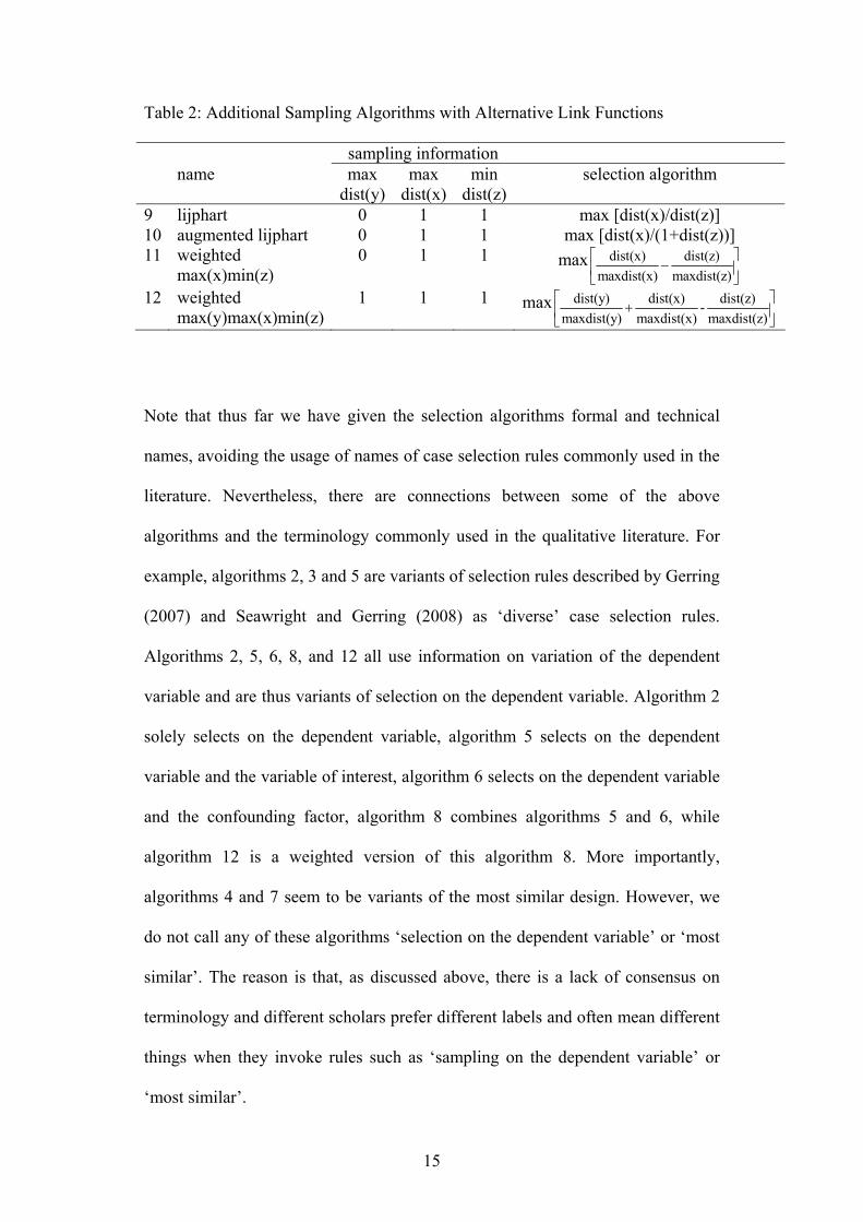
Table 2: Additional Sampling Algorithms with Alternative Link Functions

sampling information name max

dist(y)max

dist(x)min

dist(z)selection algorithm

9 lijphart 0 1 1 max [dist(x)/dist(z)] 10 augmented lijphart 0 1 1 max [dist(x)/(1+dist(z))] 11 weighted

max(x)min(z) 0 1 1 max dist(x) dist(z)

maxdist(x) maxdist(z)⎡ ⎤

−⎢ ⎥⎣ ⎦

12 weighted max(y)max(x)min(z)

1 1 1 max dist(y) dist(x) dist(z)-maxdist(y) maxdist(x) maxdist(z)⎡ ⎤

+⎢ ⎥⎣ ⎦

Note that thus far we have given the selection algorithms formal and technical

names, avoiding the usage of names of case selection rules commonly used in the

literature. Nevertheless, there are connections between some of the above

algorithms and the terminology commonly used in the qualitative literature. For

example, algorithms 2, 3 and 5 are variants of selection rules described by Gerring

(2007) and Seawright and Gerring (2008) as ‘diverse’ case selection rules.

Algorithms 2, 5, 6, 8, and 12 all use information on variation of the dependent

variable and are thus variants of selection on the dependent variable. Algorithm 2

solely selects on the dependent variable, algorithm 5 selects on the dependent

variable and the variable of interest, algorithm 6 selects on the dependent variable

and the confounding factor, algorithm 8 combines algorithms 5 and 6, while

algorithm 12 is a weighted version of this algorithm 8. More importantly,

algorithms 4 and 7 seem to be variants of the most similar design. However, we

do not call any of these algorithms ‘selection on the dependent variable’ or ‘most

similar’. The reason is that, as discussed above, there is a lack of consensus on

terminology and different scholars prefer different labels and often mean different

things when they invoke rules such as ‘sampling on the dependent variable’ or

‘most similar’.

15

We conclude the presentation and discussion of case selection algorithms

with a plea for clarity and preciseness. Rather than referring to a ‘case selection

design’, qualitative researchers should be as clear and precise as possible when

they describe how they selected cases. Qualitative research will only be replicable

if scholars provide information on the sample from which they selected cases, the

variables of interest and the confounding factors (and possibly the dependent

variable, but see the results from the MC analysis below advising against taking

variation of the dependent variable into account), and the selection algorithm they

used. Others can only evaluate the validity of causal inferences if qualitative

researchers provide all this information.

3. A Monte Carlo Analysis of Case Selection Algorithms

In this section, we explore the performance of the competing case selection

algorithms defined in the previous section with the help of Monte Carlo (MC)

experiments. After a brief introduction to MC experiments, we discuss how we

evaluate selection algorithms. We then introduce the data generating process

(DGP) and the various MC experiments for which we report results.

3.1. Monte Carlo Experiments in Qualitative Research

The method of MC experiments relies on random sampling from an underlying

DGP in order to evaluate the finite sample properties of different methods of

analysis, different estimators, or different model specifications. MC experiments

are the accepted ‘gold standard’ in quantitative research, but because of their

focus on small sample properties they are equally suitable for evaluating methods

of analysis in qualitative research – for example, for evaluating different case

selection rules, as in this paper. MC experiments provide insights both into the

16

average accuracy of estimates and therefore ex ante reliability of causal

inferences. In quantitative methodology, MC experiments compare the estimated

coefficients from a large number of randomly drawn samples to the true

coefficient, known to the researcher because she specifies the data generating

process. Deviations of the estimated coefficient from the true coefficient can

result from two sources: bias and inefficiency. While bias relates to model

misspecification, inefficiency results from a low level of information, which in

turn increases the influence of the unsystematic error on the estimates. Note that

quantitative analyses assume that the errors in the model are normally distributed

(given there is no misspecification included in the DGP). In limited samples, the

errors are likely to deviate from this assumption as a few random draws from a

perfect normal distribution reveal, but in an unknown way. On average, this

deviation diminishes with sample size.13 If such a deviation exists, the estimated

coefficient in each draw will differ from the true coefficient. Monte Carlo

analyses therefore redraw the error many times from a normal distribution in order

to measure the influence of sampling distribution on the reliability of the point

estimate.

MC analyses can analogously be used to study the ex ante reliability of

qualitative methods. Yet, one feature differs: qualitative methods do not account

for an error process. Thus, qualitative research implicitly assumes that causal

processes are deterministic. In a probabilistic world where causal effects are partly

stochastic, qualitative researchers would compute an effect of x on y that deviates

13 This logic provides the background of King et al. (1995) repeated claim that increasing

the sample size makes inferences more reliable. Yet, smaller sample make it easier to

control for heterogeneity so that a potential trade-off between efficiency and specification

error exist (Braumoeller 2003).

17

from the truth even if qualitative researchers by chance or by some superior rule

would select cases from the population regression line unless of course the error

component of both cases would also be identical by chance. On average, however,

the difference in the error component would be equal to the standard deviation of

the errors. Thus, the larger the causal effect of interest relative to the stochastic

element, the closer the computed effect gets to the true effect if we hold

everything else constant.

We are not mainly concerned here with bias resulting from the absence

of controls for an error process in qualitative research and thus do not want to

discuss whether causal processes in the social sciences will turn out to be

perfectly determined by bio-chemical processes in the brain of deciders given any

social and structural constellation. Rather, we are interested in how different case

selection algorithms deal with the potential disturbances of unaccounted noise,

(correlated) confounding factors and relative effect strengths of the variable of

interest and the confounding factors. We are dominantly interested in the relative

performance of alternative case selection algorithms.

Specifically, we define various data generating processes from which we

draw a number of random samples and then select two cases from each sample

according to a specific algorithm. As a consequence of the unaccounted error

process, the computed effects from the various MC experiments will deviate more

or less from the truth even when the selection algorithm works otherwise

perfectly. Yet, since we confront all selection algorithms with the same set of data

generating processes including the same error processes, performance differences

must result from the algorithms themselves. These differences occur because

different algorithms will select different pairs of cases i and j and as a

18

consequence, the computed effect and the distance of this effect from the true

effect differs.

3.2. Criteria for Evaluation the Performance of Selection Algorithms

We use two criteria to evaluate the performance of different case selection

algorithms. First, we compare the reliability of inference on effect strengths.

Specifically, the effect size of x on y from a comparative case study with two

cases equals

( )ˆ i

i j

y yx j

x xβ

−=

− , (1)

where subscripts [i,j] represent the two selected cases from the known population

(or sample). We take the root mean squared error (RMSE) as our measure for the

reliability of causal inference as it reacts to both bias and inefficiency. The RMSE

is defined as

( ) ( ) ( )2

2ˆ

ˆ ˆ,true

trueRMSE Var BiasN

β ββ β β

− ⎡ ⎤= = + ⎢ ⎥⎣ ⎦∑

. (2)

This criterion not only includes the influence of model misspecification on results

(the average deviation of the computed effect from the true effect, known as bias),

but also accounts for inefficiency, which is a measure of the sampling variation of

the computed effect that reflects the influence of random noise on the computed

effect. In practice, researchers cannot do anything to avoid the influence of this

random deviation from the assumed normal distribution since they cannot observe

it, but they can choose case selection algorithms (or estimation procedures in

quantitative research) that respond less to these random deviations than others.

Everything else equal, any given point estimate of a coefficient becomes more

reliable the lower the average effect of the error process on the estimation.

19

Our second criterion takes into account that qualitative researchers

typically do not compute the strength of an effect but rather analyze whether

effects have the sign predicted by theories. After all, theories usually do not

predict more than the sign of an effect and the direction of causality. For this

reason, we employ the share of incorrectly predicted effect directions as our

second criterion, which we compute according to

( )1

ˆ 0

1000

n

kk

xincorrectsign

β=

⎡ ⎤≤⎣ ⎦=∑

, (3)

where k =1…n denotes the number of iterations in which the estimated coeffi-

cients have the wrong sign. We divide by 1000 iterations – the total number of

repetitions for each experiment – in order to report ratios.

This criterion must be cautiously interpreted: a low number of incorrect

signs may result from efficient and unbiased estimates or – quite to the contrary –

from biased effects. Since we assume a coefficient of 1.0 for both the variable of

interest x and the confounding factor z, bias may reduce the share of incorrect

signs when x and z are positively correlated, but it may increase this share if x and

z are negatively correlated. We thus can easily explore how strongly algorithms

react to misspecification (bias) by comparing the share of incorrect signs when

corr(x,z)=0.9 to the share when corr(x,z)=-0.9. An unbiased selection algorithm

gives the same share of incorrect signs in both specifications. A biased selection

algorithm leads to a smaller share of incorrect signs when the correlation between

x and z is positive than when this correlation is negative.14 Thus, a selection

algorithm is not necessarily better if it produces a larger share of correctly

predicted signs but when the share of correctly predicted signs does not vary

14 Note that this is a consequence of our specific DGP, not a general truth.

20

much with the strengths of the specification problem included in the data

generating process. For example, the share of correctly predicted signs should be

high and at the same time remain unaffected by changes in the correlation

between the variable of interest x and the confounding factors z. However,

researchers should not avoid biased selection algorithms at all costs. If unbiased

estimators are far less reliable than biased estimators, researchers can make more

valid inferences using the latter (see Plümper and Troeger 2007).

3.3. The Data Generating Processes

We conducted MC experiments with both a continuous and a binary dependent

variable. As one should expect, the validity of inferences is significantly lower

with a binary dependent variable. Since otherwise results are substantively

identical we only report in detail the findings from the experiments with a

continuous dependent variable here; results for the experiments with the

dichotomous dependent variable are briefly summarized and details can be found

on the web appendix to this paper. We use a simple linear cross-sectional data

generating process for evaluating the relative performance of case selection al-

gorithms in qualitative research:

i i iy x z iβ γ= + + ε , (4)

where y is the dependent variable, x is the exogenous explanatory variable of in-

terest, z is a control variable, ,β γ represent coefficients and ε is an iid error

process. This DGP resembles what Gerring and McDermott (2007: 690) call a

‘spatial comparison’ (a comparison across n observations), but our conclusions

equally apply to ‘longitudinal’ (a comparison across t periods) and ‘dynamic com-

parisons’ (a comparison across n·t observations).

21

The variables x and z are always drawn from a standard normal

distribution, ε is drawn from a normal distribution with mean zero and standard

deviation of 1.515, and, unless otherwise stated, all true coefficients take the value

of 1.0, the standard deviation of variables is 1.0, correlations are 0.0 and the

number of observations N equals 100. We are exclusively interested in making

inferences with respect to the effect of x on y. This setup allows us to conduct

three sets of MC experiments, in which we vary the parameters of the DGP and

evaluate the effect of this variation on the precision with which the algorithms

approach the true coefficients.16 In the first set of experiments, we change the

number of observations from which the two cases are chosen (i = 1,…N), thereby

varying the size of the sample from which researchers select two cases. In the

second set of experiments, we vary the correlation between x and z, that is, the

correlation between the variable of interest and the confounding factor. In the

final set of experiments, we vary the variance of x and thus the effect size or

explanatory power of x relative to the effect size of the confounding factor z.

Analyzing the impact of varying the sample size on the validity of

inference in qualitative research may seem strange at first glance. After all,

qualitative researchers usually study a fairly limited number of cases. In fact, in

our MC analyses we generate effects by looking at a single pair of cases selected

by each of the case selection algorithms. So why should the number of

observations from which we select the two cases matter? The reason is that if

qualitative researchers can choose from a larger number of cases about which they

15 Thereby, we keep the R² at appr. 0.5 for the experiments with a continuous dependent

variable.

16 We have conducted more experiments than we can report and discuss here. The Stata do-

file with the full set of experiments is available upon request.

22

have theoretically relevant information, they will be able to select a better pair of

cases given the chosen algorithm. The more information researchers have before

they select cases the more reliable their inferences should thus become.

By varying the correlation between x and the control variable z we can

test for the impact of confounding factors on the performance of the case selection

algorithms. With increasing correlation, inferences should become less reliable.

Thereby, we go beyond the usual focus on ‘sampling error’ of small-N studies and

look at the effect of potential model misspecification on the validity of inference

in qualitative research. While quantitative researchers can eliminate the potential

for bias from correlated control variables by including these to the right-hand-side

of the regression model, qualitative researchers have to use appropriate case

selection rules to reduce the potential for bias.

Finally, in varying the standard variation of x we analyze the effect of

varying the strength of the effect of the variable of interest on the dependent

variable. The larger this relative effect size of the variable of interest, the more

reliable causal inferences should become.17 The smaller the effect of the variable

of interest x on y in comparison to the effect of the control or confounding

variables z on y, the harder it is to identify the effect correctly and the less valid

the inferences, especially when the researcher does not know the true specification

of the model.18

17 We achieve this by changing the variance of the explanatory variable x, leaving the

variance of the confounding factor z and the coefficients constant. Equivalently, one

could leave the variance of x constant and vary the variance of z. Alternatively, one can

leave both variances constant and change the coefficients of x and/or z.

18 Quantitative and qualitative methodologists usually prefer to assume that the true model

is known to the researcher, while applied researchers know that they do not know the true

model (Plümper 2010).

23

3.4 Results

In this section, we report the results of the three sets of MC analysis, i.e. in which

we vary the sample size N, vary the correlation between x and the confounding

factor z, and vary the standard variation of x. Given the simple linear DGP, these

three variations mirror the most important factors that can influence the inferential

performance of case selection algorithms. In each type of analysis we draw 1000

samples from the underlying DGP.

Table 3 reports the MC results where we only vary the size of the

sample from which we draw the two cases. In this experiment, we do not allow

for systematic correlation between the variable of interest x and the confounding

factor z. The deviations of computed effects from the true effect occur because of

‘normal’ sampling error and how efficiently the algorithm deals with the available

information.

24

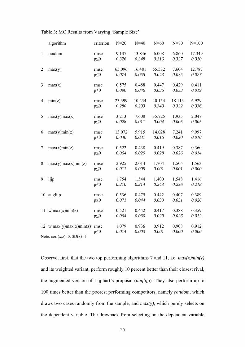
Table 3: MC Results from Varying ‘Sample Size’ algorithm criterion N=20 N=40 N=60 N=80 N=100 1

random rmse 9.137 13.846 6.008 6.860 17.349

p≤0 0.326 0.348 0.316 0.327 0.310 2

max(y) rmse 65.096 16.481 55.532 7.604 12.787

p≤0 0.074 0.055 0.043 0.035 0.027 3

max(x) rmse 0.575 0.488 0.447 0.429 0.411

p≤0 0.090 0.046 0.036 0.033 0.019 4

min(z) rmse 23.399 10.234 40.154 18.113 6.929

p≤0 0.280 0.293 0.343 0.322 0.336 5

max(y)max(x) rmse 3.213 7.608 35.725 1.935 2.047

p≤0 0.028 0.011 0.004 0.005 0.005 6

max(y)min(z) rmse 13.072 5.915 14.028 7.241 9.997

p≤0 0.040 0.031 0.016 0.020 0.010 7

max(x)min(z) rmse 0.522 0.438 0.419 0.387 0.360

p≤0 0.064 0.029 0.028 0.026 0.014 8

max(y)max(x)min(z) rmse 2.925 2.014 1.704 1.505 1.563

p≤0 0.011 0.005 0.001 0.001 0.000 9

lijp rmse 1.754 1.544 1.400 1.548 1.416

p≤0 0.210 0.214 0.243 0.236 0.218 10

auglijp rmse 0.536 0.479 0.442 0.407 0.389

p≤0 0.071 0.044 0.039 0.031 0.026 11

w max(x)min(z) rmse 0.521 0.442 0.417 0.388 0.359

p≤0 0.064 0.030 0.029 0.026 0.012 12

w max(y)max(x)min(z) rmse 1.079 0.936 0.912 0.908 0.912

p≤0 0.014 0.003 0.001 0.000 0.000 Note: corr(x,z)=0, SD(x)=1

Observe, first, that the two top performing algorithms 7 and 11, i.e. max(x)min(z)

and its weighted variant, perform roughly 10 percent better than their closest rival,

the augmented version of Lijphart’s proposal (auglijp). They also perform up to

100 times better than the poorest performing competitors, namely random, which

draws two cases randomly from the sample, and max(y), which purely selects on

the dependent variable. The drawback from selecting on the dependent variable

25

can be reduced if researchers additionally take into account variation of x and/or

variation of z, but the relevant algorithms 5, 6, 8, and 12 are typically inferior to

their counterparts 3, 4, 7, and 11, which ignore variation of y19. Accordingly,

selection on the dependent variable does not only lead to unreliable and likely

wrong inferences; using information on the dependent variable also makes other

selection algorithms less reliable. Hence, researcher should not pay attention to

the outcome when they select cases. By selecting cases on the variable of interest

x while at the same time controlling for the influence of confounding factors,

researchers are likely to choose cases which vary in their outcome if x indeed

exerts an effect on y.

Another interesting finding from table 3 is that only five algorithms

become unambiguously more reliable when the sample size from which we draw

two cases increases: max(x), max(x)min(z) and its weighted variant

wmax(x)min(z), max(y)max(x)min(z), and auglijp. Of course, algorithms need to

have a certain quality to generate visible improvements when the sample size

becomes larger. Random selection, for example, only improves on average if the

increase in sample size leads to relatively more ‘onliers’ than ‘outliers’. This may

be the case, but there is no guarantee. When researchers use relative reliable case

selection algorithms, however, an increase in the size of the sample, on which

information is available, improves causal inferences unless one adds an extreme

outlier. In fact, extreme outliers are problematic for causal inferences from

19 Algorithms 4 and 6 are an exception to this rule. Both do not take variance in the

interesting explanatory variable x into account. Algorithm 4 only minimizes the variance

of the confounding variable z while algorithm 6 maximizes in addition the variance of the

dependent variable y. This shows that selecting divers cases in x alone or in addition to

other rules increases reliability of causal inferences immensely.

26

comparative case analysis. They therefore should be excluded from the sample

from which researchers select cases.

The results so far support the arguments against random selection and

King, Keohane and Verba’s (1994) verdict against sampling on the dependent

variable, but of course qualitative researchers hardly ever select cases randomly.

Selection on the dependent variable may be more common practice, even if

researchers typically do not admit to it. If researchers know, as they typically do,

that both x and y vary in similar ways and allow this variation to guide their case

selection, then the results are likely to simply confirm their theoretical priors.

Selection rules must thus be strict and should be guided by verifiable rules rather

than discretion. Another interesting conclusion following from table 3 is that

inferences become more valid when researchers have more information before

they start analyzing cases and when they use appropriate case selection rules.

Conversely, researchers using case selection criteria unrelated to the theoretical

model such as their own language skills or the preferences of a funding agency

cannot guarantee valid inferences.

In table 4, we report the results of MC experiments from varying the

correlation between the variable of interest x and the confounding factor z.

27

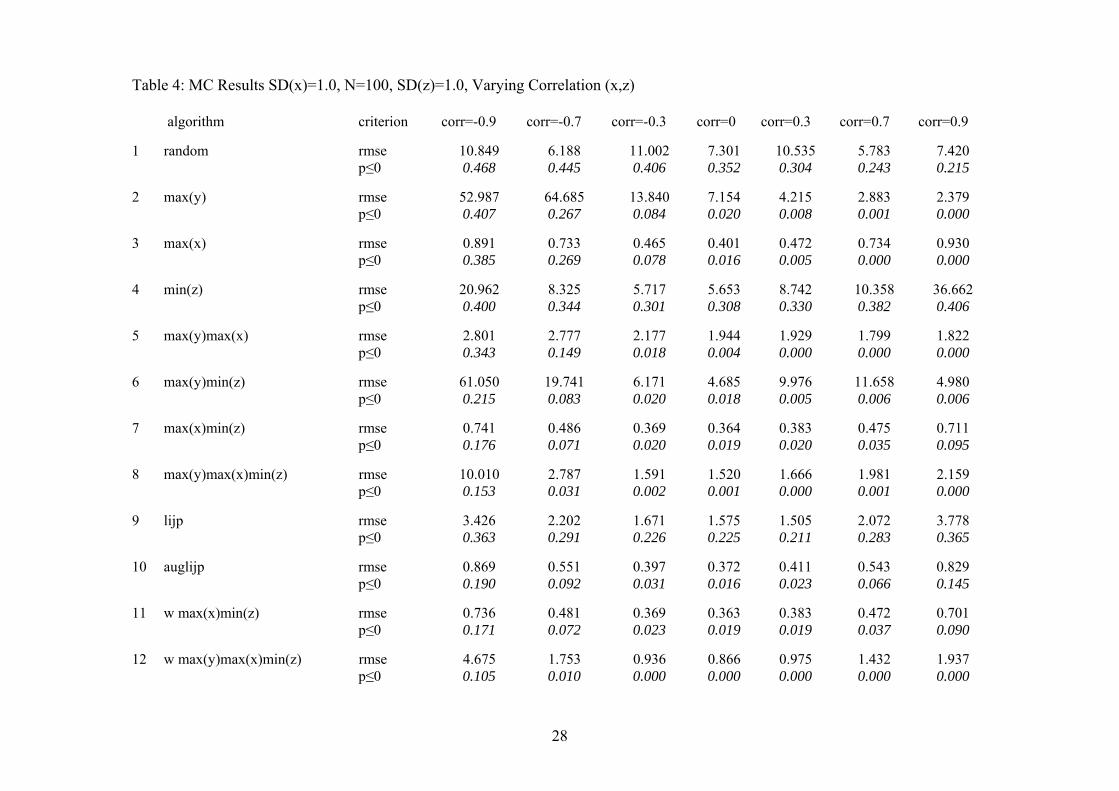
Table 4: MC Results SD(x)=1.0, N=100, SD(z)=1.0, Varying Correlation (x,z) algorithm criterion corr=-0.9 corr=-0.7 corr=-0.3

corr=0 corr=0.3 corr=0.7 corr=0.9 1 random rmse 10.849 6.188 11.002 7.301 10.535 5.783 7.420 p≤0 0.468 0.445 0.406 0.352 0.304 0.243 0.215 2 max(y) rmse 52.987 64.685 13.840 7.154 4.215 2.883 2.379 p≤0 0.407 0.267 0.084 0.020 0.008 0.001 0.000 3 max(x) rmse 0.891 0.733 0.465 0.401 0.472 0.734 0.930 p≤0 0.385 0.269 0.078 0.016 0.005 0.000 0.000 4 min(z) rmse 20.962 8.325 5.717 5.653 8.742 10.358 36.662 p≤0 0.400 0.344 0.301 0.308 0.330 0.382 0.406 5 max(y)max(x) rmse 2.801 2.777 2.177 1.944 1.929 1.799 1.822 p≤0 0.343 0.149 0.018 0.004 0.000 0.000 0.000 6 max(y)min(z) rmse 61.050 19.741 6.171 4.685 9.976 11.658 4.980 p≤0 0.215 0.083 0.020 0.018 0.005 0.006 0.006 7 max(x)min(z) rmse 0.741 0.486 0.369 0.364 0.383 0.475 0.711 p≤0 0.176 0.071 0.020 0.019 0.020 0.035 0.095 8 max(y)max(x)min(z) rmse 10.010 2.787 1.591 1.520 1.666 1.981 2.159 p≤0 0.153 0.031 0.002 0.001 0.000 0.001 0.000 9 lijp rmse 3.426 2.202 1.671 1.575 1.505 2.072 3.778 p≤0 0.363 0.291 0.226 0.225 0.211 0.283 0.365 10 auglijp rmse 0.869 0.551 0.397 0.372 0.411 0.543 0.829 p≤0 0.190 0.092 0.031 0.016 0.023 0.066 0.145 11 w max(x)min(z) rmse 0.736 0.481 0.369 0.363 0.383 0.472 0.701 p≤0 0.171 0.072 0.023 0.019 0.019 0.037 0.090 12 w max(y)max(x)min(z) rmse 4.675 1.753 0.936 0.866 0.975 1.432 1.937 p≤0 0.105 0.010 0.000 0.000 0.000 0.000 0.000

28

Note that all substantive results from table 3 remain valid if we allow for correla-

tion between the variable of interest and the confounding factor. The gap between

max(x)min(z) and its weighted variant to the next best algorithms widens slightly.

Table 4 also demonstrates that correlation between the variable of interest and

confounding factors renders causal inferences from qualitative research less reli-

able. Over all experiments and algorithms, the RMSE increases by at least 100

percent when the correlation between x and z increases from 0.0 to either -0.9 or

+0.9.

Most importantly, we can use this experiment to draw some conclusions

about the degree to which the different selection algorithms can deal with omitted

variable bias by comparing the estimates with corr(x,z)=-0.9 to the estimates with

corr(x,z)=+0.9 in terms of both the RMSE and the share of estimates with in-

corrent signs. As mentioned above, if the selection algorithm can perfectly deal

with this correlation, the RMSE and the share of estimates with an incorrect sign

should be identical for both correlations. Evaluating the performance of the

selection algorithms in this manner, we conclude that when the variable of interest

is correlated with the confounding factor, the augmented Lijphart selection

algorithm (auglijp) performs best. This algorithm combines high reliability (a low

overall RMSE) with robustness when the explanatory variables are correlated. In

comparison, max(x)min(z) has an approximately 10 percent lower RMSE, but it

suffers twice as much from correlation between the explanatory factors. The other

selection algorithms previously identified as inferior are also strongly biased,

which provides additional evidence against them.

Finally, we examine how algorithms respond to variation in the strength

of the effect of the variable of interest. Naturally, inferences from case studies

29

become generally more reliable when the variable of interest exerts a strong effect

on y relative to the effect of the confounding factors.20

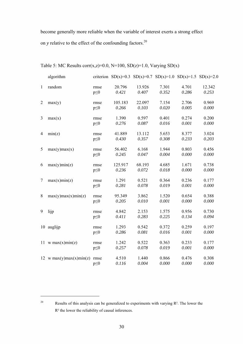
Table 5: MC Results corr(x,z)=0.0, N=100, SD(z)=1.0, Varying SD(x)

algorithm criterion SD(x)=0.3 SD(x)=0.7 SD(x)=1.0 SD(x)=1.5 SD(x)=2.0 1 random rmse 20.796 13.926 7.301 4.701 12.342 p≤0 0.421 0.407 0.352 0.286 0.253 2 max(y) rmse 105.183 22.097 7.154 2.706 0.969 p≤0 0.266 0.103 0.020 0.005 0.000 3 max(x) rmse 1.390 0.597 0.401 0.274 0.200 p≤0 0.276 0.087 0.016 0.001 0.000 4 min(z) rmse 41.889 13.112 5.653 8.377 3.024 p≤0 0.430 0.357 0.308 0.233 0.203 5 max(y)max(x) rmse 56.402 6.168 1.944 0.803 0.456 p≤0 0.245 0.047 0.004 0.000 0.000 6 max(y)min(z) rmse 125.917 68.193 4.685 1.671 0.738 p≤0 0.236 0.072 0.018 0.000 0.000 7 max(x)min(z) rmse 1.291 0.521 0.364 0.236 0.177 p≤0 0.281 0.078 0.019 0.001 0.000 8 max(y)max(x)min(z) rmse 95.349 3.862 1.520 0.654 0.388 p≤0 0.205 0.010 0.001 0.000 0.000 9 lijp rmse 4.842 2.153 1.575 0.956 0.730 p≤0 0.411 0.283 0.225 0.134 0.094 10 auglijp rmse 1.293 0.542 0.372 0.259 0.197 p≤0 0.286 0.081 0.016 0.001 0.000 11 w max(x)min(z) rmse 1.242 0.522 0.363 0.233 0.177 p≤0 0.257 0.078 0.019 0.001 0.000 12 w max(y)max(x)min(z) rmse 4.510 1.440 0.866 0.476 0.308 p≤0 0.116 0.004 0.000 0.000 0.000

20 Results of this analysis can be generalized to experiments with varying R². The lower the

R² the lower the reliability of causal inferences.

30

In table 5 we vary the standard deviation of the explanatory factor x; a small

standard deviation indicates a small effect of x on y as compared to the effect

exerted from z on y. The results show that the performance of all case selection

algorithms suffers from a low ‘signal to noise’ ratio. The smaller the effect of the

variable of interest x on y relative to the effect of z on y, the less reliable the causal

inferences from comparative case study research becomes. Yet, we find that the

algorithms which performed best in the previous two sets of experiments also turn

out to be least vulnerable to a small effect of the variable of interest. Accordingly,

while inferences do become more unreliable when the effect of the variable of

interest becomes small relative to the total variation of the dependent variable,

comparative case studies are not simply confined to analyzing the main

determinant of the phenomenon of interest if one of the high performing case

selection algorithms are used.

3.5. Additional MC Results

Before we conclude from our findings on the optimal choice of case selection

algorithms, we briefly report results from additional MC experiments which we

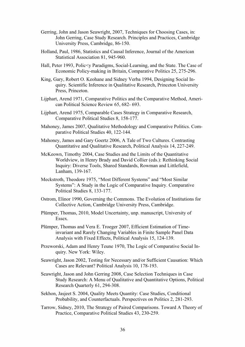
show in full in the web appendix to the paper. First, weighting x and z by their

respective sample range becomes more important when the DGP includes

correlation between x and z and the effect of x on y is relatively small (see web

appendix table 1). In this case, weighting both the variation of x and z before

using the max(x)min(z) selection rule for identifying two cases increases the

reliability of causal inferences slightly.

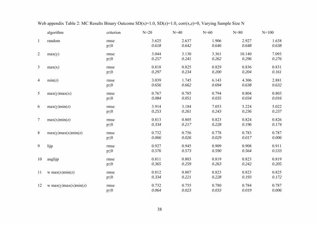
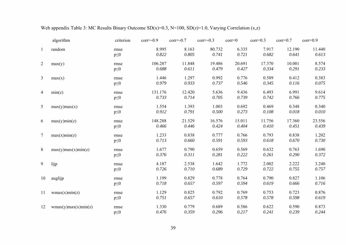
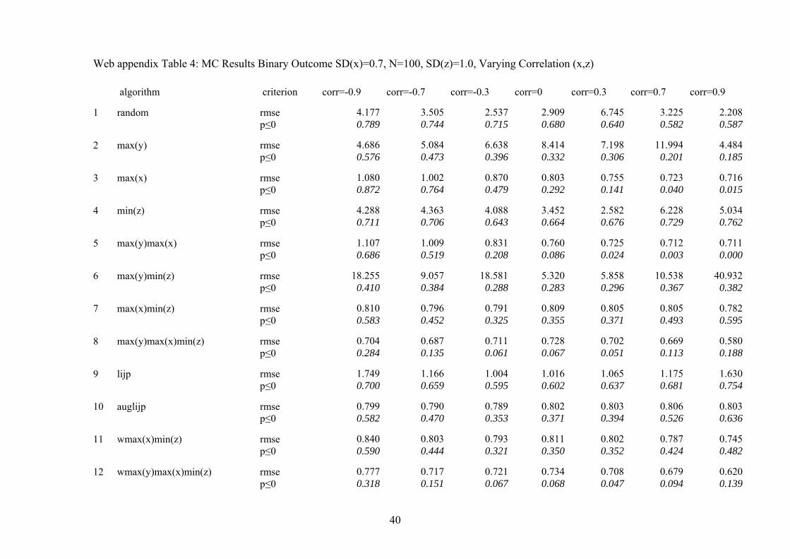
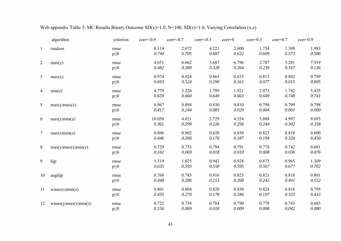
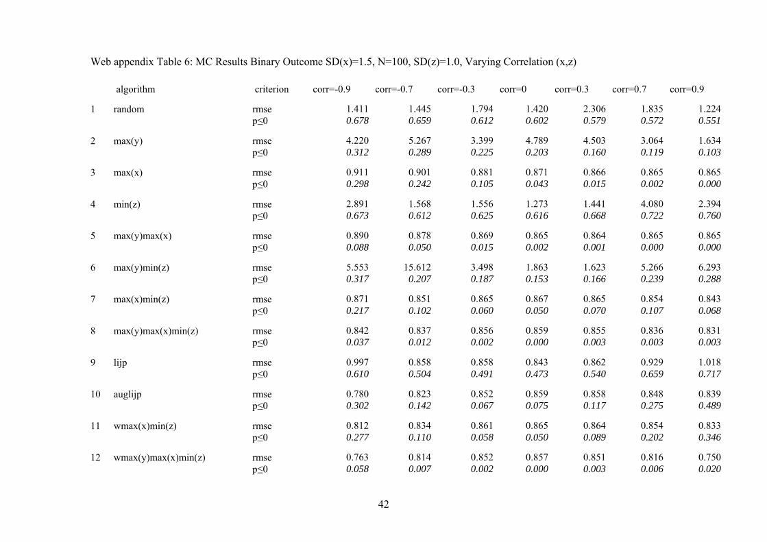
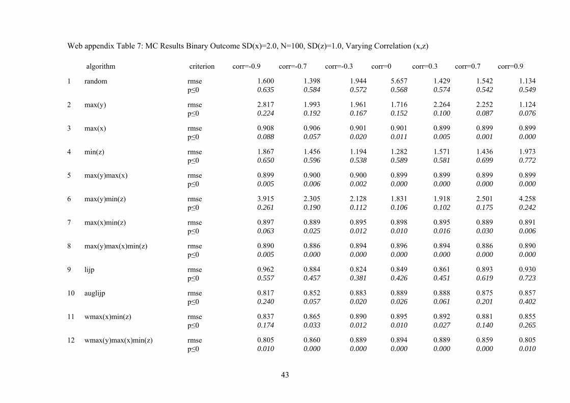
Second, we also conducted the full range of MC experiments with a

dichotomous dependent variable (see web appendix tables 2 to 7). We find that

the algorithms that perform best with a continuous dependent variable also

31

dominate with respect to reliability when we analyze dichotomous dependent

variables. Yet, causal inferences from comparative qualitative case study research

become far less reliable when the dependent variable is dichotomous for all

selection algorithms compared to the case of a continuous dependent variable. The

root mean squared error roughly doubles for the better performing algorithms. As

a consequence, causal inferences with a binary dependent variable and an

additional complication (either a non-trivial correlation between x and z or a

relatively small effect of x on y) are not reliable. Accordingly, qualitative

researchers should not throw away variation and analyze continuous or categorical

dependent variables whenever possible. Where the dependent variable is

dichotomous, qualitative research is confined to what most qualitative researchers

actually do in such situations: trying to identify strong and deterministic

relationships or necessary conditions (Dion 1998; Seawright 2002). In both cases,

the strong deterministic effect of x on y compensates for the low level of

information in the data.

3.6. Summary

Applied qualitative researchers should take away four lessons from our Monte

Carlo experiments: First, the ex ante validity of generalizations from comparative

case studies crucially depends on what we have dubbed case selection algorithms.

Second, selecting cases from a larger sample ceteris paribus gives more reliable

results. Yet, the ceteris paribus conditions need to be explored in greater detail

(we will do so in a follow-up paper). Third, ignoring information on the

dependent variable makes inferences much more reliable. Fourth, selecting cases

based on the variable of interest and confounding factors improves the reliability

of causal inferences in comparison to selection algorithms that consider just the

32

variable of interest or just confounding factors. Fifth, correlation between the

variable of interest and confounding factors renders inferences less reliable. Sixth,

inferences about relatively strong effects are more reliable than inferences about

relatively weak effects. And seventh, the reliability of inferences depends on the

variation scholars can analyze. Accordingly, throwing away information by

dichotomizing variables appears to be a particularly bad idea. A continuous

dependent variable allows for more valid inferences and a dichotomous dependent

variable should only be used if there is no alternative.

4. Conclusion

There can be no doubt that qualitative research can be used for more than making

causal inferences, but when researchers aim at generalizing their qualitative

findings, getting the selection of cases right is of the highest importance. In short:

The validity of causal inferences from qualitative research stands and falls with

the choice of a case selection rule. In order to correctly generalize findings from a

small number of cases to a larger sample or the entire universe of cases – an

exercise that qualitative researchers often conduct – researchers need to have a

good theoretical approximation of the true model and a sufficiently large sample

from which they select cases. If they then select cases in the way the best

performing algorithms in our Monte Carlo competition suggest, they have done

their best to make sure that their generalization will be correct.

We believe that our Monte Carlo study lends additional support to

guidance given by qualitative methodologists. After all, the best performing

algorithm in our analysis of alternative selection algorithms appears to be a

variant of Gerring and Seawright’s diverse design, which in turn draws on

33

Przeworski and Teune’s most similar design. In this respect, the major findings of

our study reinforce existing knowledge.

On a more general level and perhaps even more important, our research

suggests that qualitative researchers can make their research replicable by

providing sufficient information on the sample from which they select cases,

comprehensively describing the set of variables they use to select cases, and by

precisely stating the employed case selection algorithm. Given these pieces of

information, qualitative research is in principle as replicable as quantitative

analyses. At the same time, this information gives other scholars sufficient clues

about the ex ante external validity of the findings derived from comparative case

study research.

34

References

Bartels, Larry M. 2004, The Unfulfilled Promises of Quantitative Imperialism, in Henry Brady and David Collier (eds.): Rethinking Social Inquiry: Diverse Tools, Shared Standards, Rowman and Littlefield, Lanham, 69-83.

Brady, Henry E. 2004, Doing good and doing better: How far does the Quantitative Template get us? in: Henry Brady and David Collier (eds.): Rethinking Social Inquiry: Diverse Tools, Shared Standards, Rowman and Littlefield, Lanham, 53-83.

Brady, Henry E., David Collier and Jason Seawright 2006, Toward a Pluralistic Vision of Methodology, Political Analysis 14, 353-368.

Braumoeller, Bear F. and Gary Goertz 2000, The Methodology of Necessary Conditions. American Journal of Political Science 44, 844-858.

Braumoeller, Bear F. 2003, Causal Complexity and the Study of Politics, Political Analysis 11, 209-233.

Collier, David 1993, The Comparative Method, in: Ada W. Finifter (ed), Political Science: The State of the Discipline II, American Political Science Asso-ciation, Washington, 105-119.

Collier, David 1995, Translating Quantitative Methods for Qualitative Research-ers. The Case of Selection Bias, American Political Science Review 89, 461-466.

Collier, David, Henry Brady and Jason Seawright, 2004, Sources of Leverage in Causal Inference. Toward an Alternative View of Methodology, in Henry Brady and David Collier (eds.), Rethinking Social Inquiry. Diverse Tools, Shared Standards, Rowman and Littlefield, Lanham, 229-265.

Collier, David and James Mahoney 1996, Insights and Pitfalls. Selection Bias in Qualitative Research, World Politics 49, 56-91.

Collier, David, James Mahoney and Jason Seawright 2004, Claiming too much: Warnings about Selection Bias, in Henry Brady and David Collier (eds.): Rethinking Social Inquiry: Diverse Tools, Shared Standards, Rowman and Littlefield, Lanham, 85-102.

Dion, Douglas 1998, Evidence and Inference in the Comparative Case Study, Comparative Politics 30, 127-145.

Geddes, Barbara, 1990, How the Cases you Choose affect the Answers you get. Selection Bias in Comparative Politics, Political Analysis 2, 131-152.

Gerring, John and Rose McDermott 1997, An Experimental Template for Case Study Research, American Journal of Political Science 51, 688-701.

Gerring, John 2004, What is a Case Study and what is it good for? American Po-litical Science Review 98, 341-354.

Gerring, John, 2007, Case Study Research. Principles and Practices, Cambridge University Press, Cambridge.

35

Gerring, John and Jason Seawright, 2007, Techniques for Choosing Cases, in: John Gerring, Case Study Research. Principles and Practices, Cambridge University Press, Cambridge, 86-150.

Holland, Paul, 1986, Statistics and Causal Inference, Journal of the American Statistical Association 81, 945-960.

Hall, Peter 1993, Polic<y Paradigms, Social-Learning, and the State. The Case of Economic Policy-making in Britain, Comparative Politics 25, 275-296.

King, Gary, Robert O. Keohane and Sidney Verba 1994, Designing Social In-quiry. Scientific Inference in Qualitative Research, Princeton University Press, Princeton.

Lijphart, Arend 1971, Comparative Politics and the Comparative Method, Ameri-can Political Science Review 65, 682- 693.

Lijphart, Arend 1975, Comparable Cases Strategy in Comparative Research, Comparative Political Studies 8, 158-177.

Mahoney, James 2007, Qualitative Methodology and Comparative Politics. Com-parative Political Studies 40, 122-144.

Mahoney, James and Gary Goertz 2006, A Tale of Two Cultures. Contrasting Quantitative and Qualitative Research, Political Analysis 14, 227-249.

McKeown, Timothy 2004, Case Studies and the Limits of the Quantitative Worldview, in Henry Brady and David Collier (eds.): Rethinking Social Inquiry: Diverse Tools, Shared Standards, Rowman and Littlefield, Lanham, 139-167.

Meckstroth, Theodore 1975, “Most Different Systems” and “Most Similar Systems”: A Study in the Logic of Comparative Inquiry. Comparative Political Studies 8, 133-177.

Ostrom, Elinor 1990, Governing the Commons. The Evolution of Institutions for Collective Action, Cambridge University Press, Cambridge.

Plümper, Thomas, 2010, Model Uncertainty, unp. manuscript, University of Essex.

Plümper, Thomas and Vera E. Troeger 2007, Efficient Estimation of Time-invariant and Rarely Changing Variables in Finite Sample Panel Data Analysis with Fixed Effects, Political Analysis 15, 124-139.

Przeworski, Adam and Henry Teune 1970, The Logic of Comparative Social In-quiry. New York: Wiley.

Seawright, Jason 2002, Testing for Necessary and/or Sufficient Causation: Which Cases are Relevant? Political Analysis 10, 178-193.

Seawright, Jason and John Gerring 2008, Case Selection Techniques in Case Study Research: A Menu of Qualitative and Quantitative Options, Political Research Quarterly 61, 294-308.

Sekhon, Jasjeet S. 2004, Quality Meets Quantity: Case Studies, Conditional Probability, and Counterfactuals. Perspectives on Politics 2, 281-293.

Tarrow, Sidney, 2010, The Strategy of Paired Comparisons. Toward A Theory of Practice, Comparative Political Studies 43, 230-259.

36

Web appendix Table 1: MC Results Continuous Outcome SD(x)=0.3, N=100, SD(z)=1.0, Varying Correlation (x,z) algorithm criterion corr=-0.9 corr=-0.7 corr=-0.3

corr=0 corr=0.3 corr=0.7 corr=0.9 1

random rmse 20.411 26.946 25.505 20.796 43.789 49.871 31.853

p≤0 0.615 0.571 0.492 0.421 0.418 0.323 0.266 2

max(y) rmse 57.993 99.264 270.517 105.183 136.001 21.068 16.749

p≤0 0.913 0.822 0.525 0.266 0.098 0.013 0.004 3

max(x) rmse 3.021 2.402 1.572 1.390 1.610 2.524 2.908

p≤0 0.910 0.802 0.483 0.276 0.111 0.029 0.006 4

min(z) rmse 69.408 27.372 32.238 41.889 20.927 373.118 68.821

p≤0 0.482 0.460 0.425 0.430 0.453 0.441 0.459 5

max(y)max(x) rmse 21.081 49.380 83.554 56.402 32.309 13.379 11.375

p≤0 0.943 0.845 0.514 0.245 0.073 0.008 0.002 6

max(y)min(z) rmse 342.961 2005.662

105.559 125.917 197.299 86.462 99.143

p≤0 0.603 0.451 0.337 0.236 0.183 0.137 0.105 7

max(x)min(z) rmse 3.015 1.862 1.380 1.291 1.343 1.819 3.100

p≤0 0.402 0.331 0.261 0.281 0.289 0.343 0.368 8

max(y)max(x)min(z) rmse 146.883 80.848 43.529 95.349 122.412 35.729 40.032

p≤0 0.656 0.466 0.286 0.205 0.151 0.092 0.052 9

lijp rmse 11.206 7.000 4.714 4.842 5.319 7.246 11.404

p≤0 0.469 0.433 0.387 0.411 0.403 0.437 0.442 10

auglijp rmse 2.773 1.871 1.377 1.293 1.340 1.800 2.851

p≤0 0.399 0.333 0.261 0.286 0.286 0.336 0.357 11

wmax(x)min(z) rmse 2.319 1.668 1.277 1.242 1.207 1.611 2.350

p≤0 0.446 0.353 0.281 0.257 0.242 0.265 0.245 12

wmax(y)max(x)min(z) rmse 16.091 9.189 4.952 4.510 4.768 6.722 9.629

p≤0 0.676 0.391 0.179 0.116 0.095 0.065 0.020

37

Web appendix Table 2: MC Results Binary Outcome SD(x)=1.0, SD(z)=1.0, corr(x,z)=0, Varying Sample Size N algorithm

criterion N=20 N=40 N=60 N=80 N=100 1

random rmse 3.625 2.637 1.906 2.927 1.638

p≤0 0.618 0.642 0.646 0.648 0.638 2

max(y) rmse 3.044 3.130 3.361 10.140 7.093

p≤0 0.257 0.241 0.262 0.296 0.276 3

max(x) rmse 0.818 0.825 0.829 0.836 0.831

p≤0 0.297 0.234 0.200 0.204 0.161 4

min(z) rmse 3.039 1.745 6.143 4.306 2.881

p≤0 0.656 0.662 0.694 0.638 0.632 5

max(y)max(x) rmse 0.767 0.785 0.794 0.804 0.803

p≤0 0.084 0.051 0.035 0.034 0.016 6

max(y)min(z) rmse 3.914 3.184 7.053 5.224 5.022

p≤0 0.253 0.261 0.243 0.236 0.237 7

max(x)min(z) rmse 0.813 0.805 0.823 0.824 0.826

p≤0 0.334 0.217 0.228 0.196 0.174 8

max(y)max(x)min(z) rmse 0.732 0.756 0.778 0.783 0.787

p≤0 0.066 0.026 0.029 0.017 0.006 9

lijp rmse 0.927 0.945 0.909 0.908 0.911

p≤0 0.576 0.573 0.590 0.564 0.533 10

auglijp rmse 0.811 0.803 0.819 0.823 0.819

p≤0 0.365 0.259 0.263 0.242 0.205 11

w max(x)min(z) rmse 0.812 0.807 0.823 0.823 0.825

p≤0 0.334 0.221 0.228 0.193 0.172 12

w max(y)max(x)min(z) rmse 0.732 0.755 0.780 0.784 0.787

p≤0 0.064 0.023 0.033 0.019 0.006

38

Web appendix Table 3: MC Results Binary Outcome SD(x)=0.3, N=100, SD(z)=1.0, Varying Correlation (x,z) algorithm criterion corr=-0.9 corr=-0.7 corr=-0.3


random rmse 8.995 8.163 80.732 6.335 7.917 12.190 11.440

p≤0 0.822 0.805 0.741 0.721 0.682 0.641 0.613 2

max(y) rmse 106.287 11.848 19.486 20.691 17.370 10.001 8.574

p≤0 0.688 0.611 0.479 0.427 0.334 0.291 0.233 3

max(x) rmse 1.446 1.297 0.992 0.776 0.589 0.412 0.383

p≤0 0.979 0.933 0.737 0.546 0.345 0.116 0.075 4

min(z) rmse 131.176 12.420 5.636 9.436 6.493 6.991 9.614

p≤0 0.733 0.714 0.705 0.739 0.742 0.766 0.775 5

max(y)max(x) rmse 1.554 1.393 1.003 0.692 0.469 0.348 0.340

p≤0 0.912 0.791 0.500 0.273 0.108 0.018 0.010 6

max(y)min(z) rmse 148.288 21.529 16.576 15.011 11.756 17.360 23.556

p≤0 0.466 0.446 0.424 0.404 0.410 0.451 0.439 7

max(x)min(z) rmse 1.233 0.838 0.777 0.766 0.793 0.838 1.202

p≤0 0.713 0.660 0.591 0.593 0.618 0.670 0.730 8


p≤0 0.376 0.311 0.281 0.222 0.261 0.290 0.372 9

lijp rmse 4.187 2.538 1.642 1.772 2.002 2.222 3.240

p≤0 0.726 0.710 0.689 0.729 0.722 0.755 0.757 10

auglijp rmse 1.199 0.829 0.778 0.764 0.790 0.827 1.106

p≤0 0.718 0.657 0.597 0.594 0.619 0.666 0.716 11

wmax(x)min(z) rmse 1.129 0.825 0.792 0.769 0.753 0.723 0.876

p≤0 0.751 0.657 0.610 0.578 0.578 0.598 0.619 12


p≤0 0.476 0.359 0.296 0.217 0.241 0.239 0.244

39



random rmse 4.177 3.505 2.537 2.909 6.745 3.225 2.208

p≤0 0.789 0.744 0.715 0.680 0.640 0.582 0.587 2

max(y) rmse 4.686 5.084 6.638 8.414 7.198 11.994 4.484

p≤0 0.576 0.473 0.396 0.332 0.306 0.201 0.185 3

max(x) rmse 1.080 1.002 0.870 0.803 0.755 0.723 0.716

p≤0 0.872 0.764 0.479 0.292 0.141 0.040 0.015 4

min(z) rmse 4.288 4.363 4.088 3.452 2.582 6.228 5.034

p≤0 0.711 0.706 0.643 0.664 0.676 0.729 0.762 5

max(y)max(x) rmse 1.107 1.009 0.831 0.760 0.725 0.712 0.711

p≤0 0.686 0.519 0.208 0.086 0.024 0.003 0.000 6

max(y)min(z) rmse 18.255 9.057 18.581 5.320 5.858 10.538 40.932

p≤0 0.410 0.384 0.288 0.283 0.296 0.367 0.382 7

max(x)min(z) rmse 0.810 0.796 0.791 0.809 0.805 0.805 0.782

p≤0 0.583 0.452 0.325 0.355 0.371 0.493 0.595 8


p≤0 0.284 0.135 0.061 0.067 0.051 0.113 0.188 9

lijp rmse 1.749 1.166 1.004 1.016 1.065 1.175 1.630

p≤0 0.700 0.659 0.595 0.602 0.637 0.681 0.754 10

auglijp rmse 0.799 0.790 0.789 0.802 0.803 0.806 0.803

p≤0 0.582 0.470 0.353 0.371 0.394 0.526 0.636 11

wmax(x)min(z) rmse 0.840 0.803 0.793 0.811 0.802 0.787 0.745

p≤0 0.590 0.444 0.321 0.350 0.352 0.424 0.482 12


p≤0 0.318 0.151 0.067 0.068 0.047 0.094 0.139

40


0.784


random rmse 8.114 2.672 4.221 2.600 1.754 1.308 1.983

p≤0 0.744 0.705 0.687 0.632 0.609 0.573 0.586 2

max(y) rmse 4.651 6.662 3.687 6.796 2.787 3.281 7.919

p≤0 0.482 0.389 0.328 0.264 0.239 0.167 0.136 3

max(x) rmse 0.974 0.924 0.861 0.833 0.813 0.802 0.799

p≤0 0.693 0.524 0.290 0.161 0.077 0.015 0.005 4

min(z) rmse 4.779 3.220 1.789 1.921 2.073 1.742 5.435

p≤0 0.659 0.660 0.649 0.663 0.649 0.748 0.741 5

max(y)max(x) rmse 0.967 0.894 0.830 0.810 0.798 0.799 0.798

p≤0 0.417 0.244 0.083 0.029 0.004 0.001 0.000 6

max(y)min(z) rmse 10.050 4.631 2.729 4.534 3.888 4.997 9.693

p≤0 0.361 0.299 0.226 0.256 0.244 0.302 0.358 7

max(x)min(z) rmse 0.806 0.802 0.820 0.830 0.823 0.818 0.800

p≤0 0.446 0.266 0.176 0.187 0.194 0.326 0.450 8


p≤0 0.161 0.069 0.018 0.010 0.008 0.036 0.076 9

lijp rmse 1.319 1.025 0.942 0.928 0.875 0.965 1.309

p≤0 0.635 0.593 0.558 0.595 0.567 0.677 0.702 10

auglijp rmse 0.768 0.785 0.816 0.823 0.821 0.818 0.801

p≤0 0.448 0.286 0.213 0.208 0.242 0.401 0.552 11

wmax(x)min(z) rmse 0.801 0.804 0.820 0.830 0.824 0.816 0.795

p≤0 0.435 0.270 0.178 0.186 0.197 0.325 0.432 12

wmax(y)max(x)min(z) rmse 0.722 0.754 0.790 0.779 0.743 0.685

p≤0 0.156 0.069 0.018 0.009 0.008 0.042 0.080

41



random rmse 1.411 1.445 1.794 1.420 2.306 1.835 1.224

p≤0 0.678 0.659 0.612 0.602 0.579 0.572 0.551 2

max(y) rmse 4.220 5.267 3.399 4.789 4.503 3.064 1.634

p≤0 0.312 0.289 0.225 0.203 0.160 0.119 0.103 3

max(x) rmse 0.911 0.901 0.881 0.871 0.866 0.865 0.865

p≤0 0.298 0.242 0.105 0.043 0.015 0.002 0.000 4

min(z) rmse 2.891 1.568 1.556 1.273 1.441 4.080 2.394

p≤0 0.673 0.612 0.625 0.616 0.668 0.722 0.760 5

max(y)max(x) rmse 0.890 0.878 0.869 0.865 0.864 0.865 0.865

p≤0 0.088 0.050 0.015 0.002 0.001 0.000 0.000 6

max(y)min(z) rmse 5.553 15.612 3.498 1.863 1.623 5.266 6.293

p≤0 0.317 0.207 0.187 0.153 0.166 0.239 0.288 7

max(x)min(z) rmse 0.871 0.851 0.865 0.867 0.865 0.854 0.843

p≤0 0.217 0.102 0.060 0.050 0.070 0.107 0.068 8


p≤0 0.037 0.012 0.002 0.000 0.003 0.003 0.003 9

lijp rmse 0.997 0.858 0.858 0.843 0.862 0.929 1.018

p≤0 0.610 0.504 0.491 0.473 0.540 0.659 0.717 10

auglijp rmse 0.780 0.823 0.852 0.859 0.858 0.848 0.839

p≤0 0.302 0.142 0.067 0.075 0.117 0.275 0.489 11

wmax(x)min(z) rmse 0.812 0.834 0.861 0.865 0.864 0.854 0.833

p≤0 0.277 0.110 0.058 0.050 0.089 0.202 0.346 12


p≤0 0.058 0.007 0.002 0.000 0.003 0.006 0.020

42



random rmse 1.600 1.398 1.944 5.657 1.429 1.542 1.134

p≤0 0.635 0.584 0.572 0.568 0.574 0.542 0.549 2

max(y) rmse 2.817 1.993 1.961 1.716 2.264 2.252 1.124

p≤0 0.224 0.192 0.167 0.152 0.100 0.087 0.076 3

max(x) rmse 0.908 0.906 0.901 0.901 0.899 0.899 0.899

p≤0 0.088 0.057 0.020 0.011 0.005 0.001 0.000 4

min(z) rmse 1.867 1.456 1.194 1.282 1.571 1.436 1.973

p≤0 0.650 0.596 0.538 0.589 0.581 0.699 0.772 5

max(y)max(x) rmse 0.899 0.900 0.900 0.899 0.899 0.899 0.899

p≤0 0.005 0.006 0.002 0.000 0.000 0.000 0.000 6

max(y)min(z) rmse 3.915 2.305 2.128 1.831 1.918 2.501 4.258

p≤0 0.261 0.190 0.112 0.106 0.102 0.175 0.242 7

max(x)min(z) rmse 0.897 0.889 0.895 0.898 0.895 0.889 0.891

p≤0 0.063 0.025 0.012 0.010 0.016 0.030 0.006 8


p≤0 0.005 0.000 0.000 0.000 0.000 0.000 0.000 9

lijp rmse 0.962 0.884 0.824 0.849 0.861 0.893 0.930

p≤0 0.557 0.457 0.381 0.426 0.451 0.619 0.723 10

auglijp rmse 0.817 0.852 0.883 0.889 0.888 0.875 0.857

p≤0 0.240 0.057 0.020 0.026 0.061 0.201 0.402 11

wmax(x)min(z) rmse 0.837 0.865 0.890 0.895 0.892 0.881 0.855

p≤0 0.174 0.033 0.012 0.010 0.027 0.140 0.265 12


p≤0 0.010 0.000 0.000 0.000 0.000 0.000 0.010

43

44

Documents

Case Selection and Causal Inference in Qualitative Research · Case Selection and Causal Inference in Qualitative Research Thomas Plümpera, Vera E. Troegerb, and Eric Neumayerc a