Embed Size (px)
Citation preview

Novel image processing of 3D textures
Carlos López Sánchez - September 2003

Contents List of figures and tables .................................................................................................. 3 Acknowledgements............................................................................................................ 5 Abstract............................................................................................................................. 6 Chapter 1 – Introduction................................................................................................... 7
1.1 Motivation & Objectives ........................................................................................ 7 1.2 Document Organization.......................................................................................... 7
Chapter 2 - Background Theories..................................................................................... 8 2.1 Introduction ............................................................................................................ 8 2.2 Illumination direction factors ................................................................................. 8 2.3 Texture directionality taxonomy .......................................................................... 10 2.4 Texture measures.................................................................................................. 13
Chapter 3 - LBPROT operator ....................................................................................... 15 3.1 Introduction .......................................................................................................... 15 3.2 LBP Algorithm ..................................................................................................... 15 3.3 LBPROT Algorithm ............................................................................................. 16
Chapter 4 - Classification based on LBPROT outputs ................................................... 19 4.1 Patterns Distribution............................................................................................. 19 4.2 Discrimination using G Statistic........................................................................... 21
Chapter 5 – Experimental research................................................................................. 23 5.1 Introduction .......................................................................................................... 23 5.2 Output variability based on the same texture ....................................................... 25
5.2.1 Results ........................................................................................................... 25 5.2.2 Assessments................................................................................................... 27
5.3 Investigation of unidirectional textures ................................................................ 28 5.3.1 Results ........................................................................................................... 28 5.3.2 Assessments................................................................................................... 35
5.4 Investigation of bidirectional textures .................................................................. 36 5.4.1 Results ........................................................................................................... 36 5.4.2 Assessments................................................................................................... 41
5.5 Investigation of multidirectional textures............................................................. 42 5.5.1 Results ........................................................................................................... 42 5.5.2 Assessments................................................................................................... 46
5.6 G statistic experiments ......................................................................................... 47 5.6.1 Results ........................................................................................................... 47 5.6.2 Assessments................................................................................................... 49
Chapter 6 – Conclusions................................................................................................. 51 Chapter 7 – Future work................................................................................................. 52 References ...................................................................................................................... 53 Appendix A: Source code................................................................................................ 54 Appendix B: Excel format files ....................................................................................... 75

List of figures and tables Figures
Figure 2.1: Normal texture illumination disposition ....................................................................................9 Figure 2.2: Perspective that shows tilt angle ................................................................................................9 Figure 2.3: Perspective that shows slat angle ...............................................................................................9 Figure 2.4: Directionality taxonomy ..........................................................................................................11 Figure 2.5: Unidirectional material ............................................................................................................11 Figure 2.6: Bidirectional material...............................................................................................................12 Figure 2.7: Multidirectional material..........................................................................................................12 Figure 3.1: LBP operation ..........................................................................................................................15 Figure 3.2: LBPROT operation ..................................................................................................................17 Figure 3.3: LBPROT rotation procedure....................................................................................................18 Figure 4.1: LBPROT output when applied on 1.acc.0.45.90 texture..........................................................19 Figure 4.2: Pattern statistical matching for 1.acc.0.45.90 texture...............................................................20 Figure 5.1: Main texture used for experimental work ................................................................................23 Figure 5.2: Distribution of LBPROT trace for texture 0.aaa.0.45.90 .........................................................25 Figure 5.3: Variability of LBPROT for unidirectional textures with slant 45º and tilt 90º ........................26 Figure 5.4: Variability of LBPROT for bidirectional textures with slant 45º and tilt 90º ..........................26 Figure 5.5: Variability of LBPROT for multidirectional textures with slant 45º and tilt 90º .....................27 Figure 5.6: Graphical behaviour of pattern 14 in 0.acc.0.45.x textures by rows ........................................28 Figure 5.7: Graphical behaviour of pattern 14 in 0.acc.0.60.x textures by rows ........................................29 Figure 5.8: Graphical behaviour of pattern 14 in 0.acc.0.75.x textures by rows ........................................29 Figure 5.9: Graphical behaviour of pattern 14 in 0.acc.0.45.x textures by columns ..................................29 Figure 5.10: Graphical behaviour of pattern 14 in 0.acc.0.60.x textures by columns ................................30 Figure 5.11: Graphical behaviour of pattern 14 in 0.acc.0.75.x textures by columns ................................30 Table 5.2: Behaviour of pattern 14 before 0.acc.0.45.x textures tilt angle shifts .......................................31 Figure 5.13: Graphical behaviour of pattern 14 in 0.acc.0.60.x textures when synchronized by columns.31 Figure 5.14: Graphical behaviour of pattern 14 in 0.acc.0.75.x textures when synchronized by columns.32 Figure 5.15: Graphical representation of table 5.3 order by minimum value (0.acc.0.45.x texture) ..........34 Figure 5.16: Graphical representation of table 5.3 order by maximum value (0.acc.0.45.x texture)..........34 Figure 5.17: Graphical behaviour of pattern 14 in 7.adj.0.45.x textures by rows.......................................35 Figure 5.18: Graphical behaviour of pattern 14 in 2.ach.0.45.x textures by rows......................................36 Figure 5.19: Graphical behaviour of pattern 14 in 2.ach.0.60.x textures by rows......................................36 Figure 5.20: Graphical behaviour of pattern 14 in 2.ach.0.75.x textures by rows......................................37 Figure 5.21: Graphical behaviour of pattern 14 in 2.ach.0.45.x textures by columns ................................37 Figure 5.22: Graphical behaviour of pattern 14 in 2.ach.0.60.x textures by columns ................................38 Figure 5.23: Graphical behaviour of pattern 14 in 2.ach.0.75.x textures by columns ................................38 Figure 5.24: Graphical behaviour of pattern 14 in 2.ach.0.45.x textures when synchronized by columns 38 Figure 5.25: Graphical behaviour of pattern 14 in 2.ach.0.60.x textures when synchronized by columns 39 Figure 5.26: Graphical behaviour of pattern 14 in 2.ach.0.75.x textures when synchronized by columns 39 Figure 5.27: Graphical behaviour of pattern 14 in 6.afe.0.45/60.x textures when synchronized by columns....................................................................................................................................................................39 Figure 5.28: Graphical behaviour of pattern 14 in 2.ach.0.45.x textures order by min values ...................40 Figure 5.29: Graphical behaviour of pattern 14 in 2.ach.0.45.x textures order by max values ..................40 Figure 5.30: Graphical behaviour of pattern 14 in 6.afe.0.45.x textures order by min values....................40 Figure 5.31: Graphical behaviour of pattern 14 in 6.afe.0.45.x textures order by max values ...................41 Figure 5.32: Graphical behaviour of pattern 14 in 0.aar.0.45.x textures by rows.......................................42 Figure 5.33: Graphical behaviour of pattern 14 in 0.aar.0.60.x textures by rows.......................................42 Figure 5.34: Graphical behaviour of pattern 14 in 0.aar.0.75.x textures by rows.......................................42 Figure 5.35: Graphical behaviour of pattern 14 in 0.aar.0.45.x textures by columns.................................43 Figure 5.36: Graphical behaviour of pattern 14 in 0.aar.0.60.x textures by columns.................................44 Figure 5.37: Graphical behaviour of pattern 14 in 0.aar.0.75.x textures by columns.................................44 Figure 5.38: Graphical behaviour of pattern 14 in 0.aar.0.45.x textures when synchronized by columns .44 Figure 5.39: Graphical behaviour of pattern 14 in 0.aar.0.60.x textures when synchronized by columns .44 Figure 5.40: Graphical behaviour of pattern 14 in 0.aar.0.75.x textures when synchronized by columns .45

Figure 5.41: Graphical behaviour of pattern 14 in 0.aaa.0.45/75.x textures when synchronized by columns....................................................................................................................................................................45 Figure 5.42: Graphical behaviour of pattern 14 in 0.aar.0.45.x textures order by min values....................46 Figure 5.43: Graphical behaviour of pattern 14 in 0.aar.0.45.x textures order by max values ...................46 Figure 5.44: G statistic behaviour for unidirectional textures used as samples ..........................................48 Figure 5.45: G statistic behaviour for bidirectional textures used as samples ............................................49 Figure 5.46: G statistic behaviour for multidirectional textures used as samples.......................................49
Tables Table 3.1: 36 possible 8-bit rotation-invariant patterns..............................................................................17 Table 5.1: Pattern 14 rows for 0.acc.0.45.x textures ..................................................................................28 Table 5.3: Maximum and minimum values for table5.1 (0.acc.0.45.x texture)..........................................33 Table 5.4: Values of table 5.3 order by minimum value (0.acc.0.45.x texture)..........................................33 Table 5.5: Values of table 5.3 order by maximum value (0.acc.0.45.x texture).........................................34 Table 5.6: G statistic results for four parts of AAA texture........................................................................47

Acknowledgements
In order to finish this project not only a lot of personal effort was required, but also the support of the people I love. For this reason firstly I want to dedicate this dissertation to my family with all my love, especially to my parents who have been the main characters of this play.
I would also like to transmit my gratitude to my “second family”, the
people I have met this year in Heriot-Watt University, especially to Javier Ormazabal (spiderguy, Euup!!), Adriana Pérez (my dear biscuit personal advisor), Vicente J. Jiménez (DJ in live) and of course, Victoria Sánchez (my beloved official English teacher picatxu version) for their essential company along this academic course. All of you have an untouchable place in the deepest of my heart forever.
Finally, and not for it less important, I would rather thank to my
supervisor – Mike Chantler – for the vital help and guidance he provided me with throughout this project’s development. Likewise, I would like to express my gratitude to all the teachers and friends (José Palacios, Agustín Caminero and the unbeatable knight, Diego Guerrero, among many others) I know in Albacete, my other home.
A million of thanks to all.

Abstract
A new invariant-rotation texture operator, known as LBPROT (Local Binary
Pattern Rotation-Invariant), has been recently developed by M. Pietikäinen, T.
Ojala and Z. Xu1. It has demonstrated much better performance at classifying
textures than the well-known CSAR (Circular-Symmetric Autoregressive Random
Field). This paper extends the experiments carried out then, and boards an
alternative series of experiments in order to find out further information regarding
LBPROT operator’s behaviour.
Among the experiments performed, an analysis of the operator’s variability
before distinct samples of the same texture2 under equal illumination conditions
was accomplished. Furthermore, a research aiming at understanding the
operator’s response when applied to different directionality features is widely
presented. Moreover, some extra experiments utilize the operator output
distribution to classify textures by using the G Statistic log-likelihood pseudo-
metric. Finally, all these investigations are assessed leading to a series of
interesting results which are discussed in depth.
1 Machine Vision and Media Processing Group, Infotech Oulu University of Oulu, P.O. Box 4500 , FIN-90401 Oulu, Finlan www.mediateam.oulu.fi/publications/pdf/7.pdf - 18 Ago 2003 2 SCOPE is the format used along the development of the experiments carried out in this paper. http://www.cee.hw.ac.uk/~mjc/scope/scope/info_centre.htm

Novel image processing of 3D textures
Chapter 1 – Introduction 7
Chapter 1 – Introduction
1.1 Motivation & Objectives
Many applications in real life require image classification techniques. Following
this we can find examples such as submarine inspection, defects detection and aerial
image acquisition. In order to deal with that requirement, classification operators are
commonly used in texture discrimination. A desirable characteristic in most of texture
operators is rotation-invariant features what facilitates the process of discrimination
considerably. LBPROT is an invariant-rotation operator presented in [1] which has
already demonstrated its outstanding characteristics at classifying
The objective of this paper is to extend the work performed so far and collaborate
to find out novel features by means of the realization of new experiments. The research
carried out in this project takes into account the nature of each texture and the factors
they are exposed to throughout the nearly 400 texture images analysed, in an effort of
particularizing the behaviour of LBPROT texture operator before particular conditions.
1.2 Document Organization
This paper starts making mention of the motives and objectives which lie on this
project’s development. Next, essential background theories are presented in order to
understand later sections. Then the following section shows a study in depth of
LBPROT texture operator where not only its operation is described, but also how to
overcome certain problems will face with. Next, we will study how to process the
LBPROT outputs in line with our objectives at image classification by analysing pattern
distributions and applying G statistic, a log-likelihood pseudo-metric. Afterwards,
several experiments are presented in the following section where the major part of this
project is developed. A by-directional-properties study is carried out describing how the
LBPROT operator behaves before the diverse conditions it was subject to. Likewise,
LBPROT variability and G statistic results will provide further information regarding
texture discrimination by using pattern distribution. After that, the last but one section
depicts the conclusions, reached assessments and achieved merits throughout this
project’s development. Finally, the last section points out the future work which might
be done according to the limitations this project was subjected to.

Novel image processing of 3D textures
Chapter 2 - Background Theories 8
Chapter 2 - Background Theories
2.1 Introduction
In this chapter several essential elements will be studied due to their great
importance in the development of the present project. Firstly, the different kinds of
illumination angles commonly used will be boarded just in the next section. There, we
will identify all the flavours and differences, as well as the manner in which they impact
in the imaging process acquisition by altering the appearance of the resultant image. The
quality of the latter’s outputs is extremely important in order to achieve a more
satisfying classification outcomes independently of the algorithm used for this purpose.
In the following section, we will deal with the directionally concept per se by
understanding not only their taxonomy, but also how it affects to our aim at imaging
classification. Besides, it will also be mentioned the intrinsic subjectiveness which this
taxonomy is subjected to.
Finally, the last section will present an overview of the different kinds of texture
measures, as a more detailed description would exceed the aims of this research as well
as it would take the reader through a series of unneeded theories to understand the
investigations carried out in this project. This section will also lead to the next chapter,
where the main pillar of this research, the LBPROT operator, is thoroughly studied.
2.2 Illumination direction factors
Illumination direction factors are essential when dealing with image classification
due to the alterations that they may cause upon the appearance of a particular kind of
texture. Additionally, illumination factors - which a particular sort of texture is exposed
to - provoke shadows or darkened regions which alter enormously many imaging
classification algorithms’ outputs leading them to obtain miserable outcomes. Hence,
effective imaging classification algorithms must take these factors into account at every
moment in order to achieve successful results. Consequently, the most outstanding

Novel image processing of 3D textures
Chapter 2 - Background Theories 9
variables involved in illumination behaviour, well known as tilt and slant angles, are
presented as follows.
Figure 2.1: Normal texture illumination disposition
The tilt angle is represented by τ symbol. It is defined as the angle formed by the
illumination projection vector with respect to the X-Y plane. Let us see the illustration
shown below:
Figure 2.2: Perspective that shows tilt angle
Likewise, slant angle is represented by σ symbol. It is defined as the angle
formed by the illuminat normal vector respect the Z-axis. The illustration shown below
depicts that angle graphically:
Figure 2.3: Perspective that shows slat angle
X
Z
Y
Texture
X
Y
Illuminant
τ
Texture
X
Z
Illuminant
σ Texture (height/relief map)

Novel image processing of 3D textures
Chapter 2 - Background Theories 10
2.3 Texture directionality taxonomy
When working on image classification, another important factor to take into
account at every moment is directionality, since each texture has specific physical
qualities or idiosyncrasies which draw a particular material to behave unequally from
another. Although any set of materials can be classified according to many features, the
terms of isotropy and anisotropy are widely used in an effort of distinguishing materials
with heterogeneous directionality characteristics. Unfortunately, there seems not to be
an agreed universal definition for those terms, and although all of them keep the same
essential meaning, they have certain subjective influence coupled to other particular
factors. Therefore, the development of the present taxonomy will be carried out
according to the aforementioned considerations.
The term of directionality makes reference to how a particular material’s particles
are prone to distribute across the surface. This definition leads us to the second level of
our taxonomy which encompasses two important elements aforementioned: isotropy
and anisotropy. A given material is said to be isotropic if its particles are uniformly
distributed in all directions. Conversely, a material is stereotyped as anisotropic if its
particles do not follow a uniform distribution in all directions.
This taxonomy goes farther in the material classification by means of the
inclusion of a third level which comprehends the terms of unidirectionality,
bidirectionality and multidirectionality. In this manner, a material is said to have
unidirectional properties if all its particles are prone to distribute in the same direction.
Obviously, a material which is considered as unidirectional, it is also isotropic at the
same time. Likewise, a material whose particles are distributed mainly in two directions
is said to be bidirectional. In all other cases which a material’s directionality cannot be
classified within the terms of neither unidirectionality nor bidirectionality, we say that
the given material has multidirectional properties, what means that its particles are
spread according to more than two directions. Evidently, both bidirectional and
multidirectional materials are considered to be anisotropic at the same time, as they do
not have a unique particle direction. Nonetheless, there are some individuals who may
consider bidirectionality to be a particular case of multidirectionality, instead of the

Novel image processing of 3D textures
Chapter 2 - Background Theories 11
view adopted in this paper. For more clarity with regards to this taxonomy, please note
the chart illustrated below:
Figure 2.4: Directionality taxonomy
The examples shown below are visual illustrations of how materials can be
classified by using the present taxonomy:
Unidirectional: ADJ
Figure 2.5: Unidirectional material
Directional
Isotropic Anisotropic
Unidireccional (=1) Bidirectional (=2) Multidirectional (+2)

Novel image processing of 3D textures
Chapter 2 - Background Theories 12
Bidirectional: ACH Polystyrene
Figure 2.6: Bidirectional material
Multidirectional: AAA Plaster fracture. How many directions are detected in the below
texture? More than two definitively…
Figure 2.7: Multidirectional material
So far, the reader might have thought of the flexibility of these terms as for
example, in the figure 2.5 the direction of particles is not absolutely unique and some
deviations are clearly observed. This leads us to state once more what at the beginning
of this section was mentioned, the subjectiveness which those terms are subjected to.

Novel image processing of 3D textures
Chapter 2 - Background Theories 13
2.4 Texture measures
Nowadays, there are many operators used to discriminate textures. Each of these
operators has different properties and provides different results, as they are based on
distinct mathematical procedures normally close related to statistics theory. Typically
these operators require a particular window size (most used 3x3) where to be applied in
order to obtain the value associated to, commonly, the centre pixel of such a window.
Operators which perform their computations by using the aforementioned way of
proceeding are called measures based on centre-symmetric auto-correlation. SAC and
SRAC are two examples in this current which are locally grey-scale invariant as well as
rotation-invariant, providing very discriminating information about the amount of local
texture. SCOV is another operator which is obtained by using the two previous
operators with a related covariance measure. Besides, it is a good measure of local
pattern contrast and provides more texture information than SAC and SRAC operators,
although is not rotation-invariant. SAC can be defined in terms of SCOV and
covariance (σ2) as shown below:
∑ −′−=4
))((41
iii xxSCOV µµ (1)
where xi and ix′ are pixels and µ is the mean.
2σSCOVSAC = (2)
SRAC behaves better than SAC before images with noise and monotonic shifts in
the grey scale. Like SAC, SRAC is also bound between values -1 and 1, as can be
inferred from the following formulas:
mm
TrrSRAC i
xii
−
+′−
−=∑
3
42)(12
1 (3)

Novel image processing of 3D textures
Chapter 2 - Background Theories 14
∑ −=l
iiix ttT )(
121 3 (4)
where in a given nxn neighbourhood with 4 centre-symmetric pairs of pixels, m is
n2 and ti is the number of ties at position ri in a ranking neighbourhood.
Unlike the previous technique, there are other operators based in grey level
difference method that have been used with successful results in some applications and
comparatives researches by using histograms of absolute difference between pairs of
grey levels. For instance, DIFF4 can be considered as a well known example of an
operator based on this technique.
The LBPROT operator, main pillar of this project, will be boarded in depth in the
next section. Likewise, there are many others operators unmentioned in this section, as
they go beyond the purpose of this paper. If the reader wishes to find out further
information in this respect, please see [1].

Novel image processing of 3D textures
Chapter 3 - LBPROT operator 15
Chapter 3 - LBPROT operator
3.1 Introduction
In this chapter we will understand how LBP (Local Binary Pattern) works at
classifying textures, as well as we will know its flaws and the way of overcoming some
of these problems. In the last section, LBPROT (Local Binary Pattern Rotation-
Invariant) will be described, taking as a base the LBP algorithm plus series of
improvements performed on it in order to achieve Rotation-Invariant features.
3.2 LBP Algorithm
LBP is a very straightforward texture operator for classifying textures by
operating on 3x3 neighbourhoods (also called windows) thresholded at the value of the
central pixel. This leads to a 0’s and 1’s matrix where 0’s occur if the neighbour pixel is
less than the threshold and 1’s do otherwise. Subsequently, the values of the last matrix
are multiplied by binomial weights dispose in increasing-value-row order. Finally, the
resultant values are summed to give place to the LBP operator’s output for the given
threshold. For a more illustrative understanding, let us show the following example
where LBP texture operator is applied:
8 4 12 1 0 1 1 2 4 1 0 4 3 6 6 0 1 8 16 0 16 1 5 9 0 0 1 32 64 128 0 0 128
(a)
(b)
(c)
(d)
Figure 3.1: LBP operation
In (a) it is shown a possible base matrix where the 6 value is considered as
threshold element (shadowed centre pixel) as it is in the centre of the matrix. By
comparing the threshold with each neighbour pixel, we obtain the matrix shown in (b).
Afterwards, every item of the matrix (b) is then multiplied by its homologous one in the
binomial weight matrix (c) both with the same coordinate. As a result the matrix (d) is
generated and by simply summing the resultant values, we obtain the value associated

Novel image processing of 3D textures
Chapter 3 - LBPROT operator 16
to the given threshold, which in this particular case is LBP=1+4+16+128=149. The
process obviously is equally applied to the rest of the pixels of the given texture.
Once this operator is being used, it comes up an unanswered question so far: how
to apply the LBP texture operator to the edges of the texture? To answer this question
several alternatives can be equally chosen, depending more on personal or professional
interests than in any other kind of considerations. The first alternative could just be not
to apply the operator to the edges of the texture. Although this is the simplest solution, it
will very likely alter slightly the final results. For it, another choice might consist in
applying the algorithm on as many pixels as possible, adopting a default value for those
which can not be mapped due to their inexistence. Likewise, a third choice can be taken
by supposing the texture was conceived in spherical shape in order to compute all pixels
across the texture. This option could be widely used in texture with good continuity
among edges, becoming probably a bad choice in those cases where continuity among
edges is not good enough. Although this choice is obviously the most complex to
accomplish, it should not extend this complexity long farther.
The choice adopted in the implementation3 of LBPROT - studied in detail just in
the next section - has been the fist one, which is to skip edges and leave them unused as
a threshold. Nonetheless, it is important to remark that this implementation use a mxn
image and outputs (m-2)x(n-2) distribution, as the original image’s edges are only used
within the calculation process and do not take part of the final result in an effort of
reducing the errors as much as possible.
3.3 LBPROT Algorithm
There are certain studies and/or applications which require a rotation-invariant
operator, what means the operator behaves quite uniformly before changes in the slant
and/or tilt angles. The LBP texture operator studied in the previous section is easily
implemented and quickly can compute a big deal of pixels which is highly desirable.
However, it is not rotation-invariant which makes it inappropriate for the
aforementioned purposes. A possible solution to equip this operator with such 3 The reader might know in detail how this implementation is as it is attached for his or her entire disposition in the Appendix A .

Novel image processing of 3D textures
Chapter 3 - LBPROT operator 17
functionally was presented in [1]. It consists in using the values obtained by the LBP
texture operator, to make an arbitrary number of rotations until every one matches with
one of the 36 pre-established patterns. These patterns are all the 36 possible different
rotation-invariant combinations of 8 bits which can be obtained by just using 8 bits
word size. For instance, the binary word 00000001 represents all words with just one bit
valued to 1. In addition, an index is attached to each pattern in order to use it as a
feature value which describes the LBP rotation-invariant features for the given
neighbourhood matrix. The 36 patterns are illustrated below using a zero-based index:
Pattern Index Pattern Index
00000000 0x00 0 00011011 0x1B 18 00000001 0x01 1 00110011 0x33 19 00000011 0x03 2 01010101 0x55 20 00000101 0x05 3 01010011 0x53 21 00001001 0x09 4 01010110 0x56 22 00010001 0x11 5 00011111 0x1F 23 00000111 0x07 6 00101111 0x2F 24 00001011 0x0B 7 01001111 0x4F 25 00010011 0x13 8 00110111 0x37 26 00100011 0x23 9 01100111 0x67 27 01000011 0x43 10 01010111 0x57 28 00010101 0x15 11 01011011 0x5B 29 00100101 0x25 12 00111111 0x3F 30 01001011 0x4B 13 01011111 0x5F 31 00001111 0x0F 14 01101111 0x6F 32 00010111 0x17 15 01110111 0x77 33 00100111 0x27 16 01111111 0x7F 34 01000111 0x47 17
11111111 0xFF 35
Table 3.1: 36 possible 8-bit rotation-invariant patterns
In order to improve the understanding of LBPROT texture operator, the same
neighbourhood matrix as used in the previous section’s example will be utilized once
more for the following LBPROT operation illustration:
8 4 12 1 0 1 3 6 6 0 1 1 5 9 0 0 1
(a)
(b)
Figure 3.2: LBPROT operation
Novel image processing of 3D textures
Chapter 3 - LBPROT operator 18
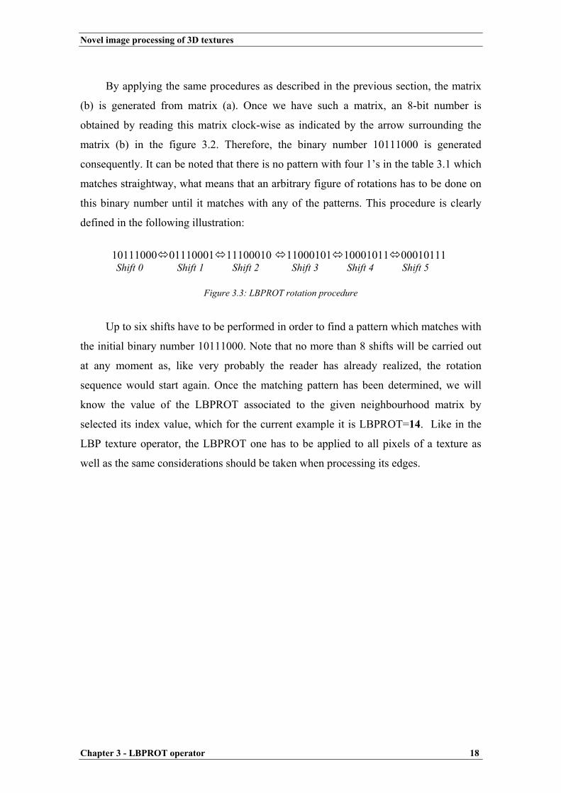
By applying the same procedures as described in the previous section, the matrix
(b) is generated from matrix (a). Once we have such a matrix, an 8-bit number is
obtained by reading this matrix clock-wise as indicated by the arrow surrounding the
matrix (b) in the figure 3.2. Therefore, the binary number 10111000 is generated
consequently. It can be noted that there is no pattern with four 1’s in the table 3.1 which
matches straightway, what means that an arbitrary figure of rotations has to be done on
this binary number until it matches with any of the patterns. This procedure is clearly
defined in the following illustration:
10111000 01110001 11100010 11000101 10001011 00010111
Shift 0 Shift 1 Shift 2 Shift 3 Shift 4 Shift 5
Figure 3.3: LBPROT rotation procedure
Up to six shifts have to be performed in order to find a pattern which matches with
the initial binary number 10111000. Note that no more than 8 shifts will be carried out
at any moment as, like very probably the reader has already realized, the rotation
sequence would start again. Once the matching pattern has been determined, we will
know the value of the LBPROT associated to the given neighbourhood matrix by
selected its index value, which for the current example it is LBPROT=14. Like in the
LBP texture operator, the LBPROT one has to be applied to all pixels of a texture as
well as the same considerations should be taken when processing its edges.

Novel image processing of 3D textures
Chapter 4 - Classification based on LBPROT outputs 19
Chapter 4 - Classification based on LBPROT outputs
4.1 Patterns Distribution
In this section we will face with how to use the texture operator’s output
mentioned in the last section – LBPROT – in order to discriminate a set of
heterogeneous textures under different illumination conditions. To achieve this purpose,
the algorithm LBPROT has been implemented to generate a particular distribution for
each texture. Each distribution might be seen as a sequence of numbers valued between
0 and 35, where every one of these values corresponds with the LBPROT operator’s
output for each thresholded window respectively. Let us show in the following example
a short piece of the output generated by the LBPROT operator when applied to the
1.acc.0.45.90 texture:
Figure 4.1: LBPROT output when applied on 1.acc.0.45.90 texture
During the computation process of a texture by using LBPROT operator, several
shifts have to be performed until the 8-bit neighbourhood number associated with each
particular pixel matches with any of 36 pre-established patterns (see table 3.1). At this
point there is another important source of information, which as it will be shown later,
can also be utilized within the classification process we aim at. It consists in counting
not only how many matches have been carried out for each pattern, but also how many
of them occurred in the first shift, how many of them occurred in the second one and so
on. Now we dispose of bigger deal of information which allows us to perform a finer
discrimination process, as a more detailed distribution is available for each texture.
23 23 23 14 2 1 6 6 14 34 6 2 14 14 14 2 6 14 23 14 14 23 3 23 17 23 30 9 14 14 1 14 23 30 23 35 30 34 6 14 6 1 23 23 30 30 14 6 23 2 34 6 2 1 14 34 14 14 1 6 6 1 0 14 14 14 14 32 14 14 23 23 14 0 2 23 6 27 0 26 34 6 34 14 6 2 30 23 34 6 0 14 30 2 2 30 23 23 0 23 30 23 …

Novel image processing of 3D textures
Chapter 4 - Classification based on LBPROT outputs 20
The statistical results of such distributions are depicted in the example show below
for 1.acc.0.45.90 texture:
Figure 4.2: Pattern statistical matching for 1.acc.0.45.90 texture
From the above figure several interesting results deserve to be studied in greater
depth. For instance, both the pattern 0 and 35 have all matches in the first shifts, leaving
the rest as zero valued. The reason of this behaviour can be revealed as simply as
analysing the rotation process which those patterns follow along their computation.
Therefore, from the table 3.1 afore presented, it is well know that the pattern 0
corresponds with the binary sequence 00000000 whereas the pattern 35 to its
complementary, which is 11111111. Once this data is noted, it is obvious comprehend
that these patterns are rotation invariant, as they keep their values unaltered before any
arbitrary number of shifts. Likewise, the patterns 5, 19, 20 and 33, which binary
PATTERN STATISTICS: ------------------- Pattern 0 --> 7884 0 0 0 0 0 0 0 total = 7884 (3.031%) Pattern 1 --> 1475 1348 1818 1300 1569 1260 2263 1253 total = 12286 (4.724%) Pattern 2 --> 2025 2100 1760 1815 2352 2176 1865 1767 total = 15860 (6.098%) Pattern 3 --> 407 454 311 220 348 406 351 252 total = 2749 (1.057%) Pattern 4 --> 163 258 205 150 157 224 207 122 total = 1486 (0.571%) Pattern 5 --> 136 137 509 129 0 0 0 0 total = 911 (0.350%) Pattern 6 --> 4232 7655 3447 3984 5580 7511 4108 2621 total = 39138 (15.047%)Pattern 7 --> 213 398 269 216 219 316 341 199 total = 2171 (0.835%) Pattern 8 --> 159 165 245 129 150 162 261 131 total = 1402 (0.539%) Pattern 9 --> 140 161 142 229 148 158 132 265 total = 1375 (0.529%) Pattern 10 --> 303 169 242 288 302 230 237 377 total = 2148 (0.826%) Pattern 11 --> 31 63 86 59 54 56 99 56 total = 504 (0.194%) Pattern 12 --> 24 29 26 19 22 24 30 37 total = 211 (0.081%) Pattern 13 --> 40 31 26 32 21 23 40 38 total = 251 (0.097%) Pattern 14 --> 4329 16921 7567 4775 8563 10831 11976 4705 total = 69667 (26.785%) Pattern 15 --> 224 395 383 242 300 356 419 246 total = 2565 (0.986%) Pattern 16 --> 175 242 169 110 186 244 156 135 total = 1417 (0.545%) Pattern 17 --> 460 433 271 266 355 392 251 244 total = 2672 (1.027%) Pattern 18 --> 181 160 220 156 150 172 228 142 total = 1409 (0.542%) Pattern 19 --> 147 126 107 91 0 0 0 0 total = 471 (0.181%) Pattern 20 --> 20 14 0 0 0 0 0 0 total = 34 (0.013%) Pattern 21 --> 31 31 49 28 32 34 39 26 total = 270 (0.104%) Pattern 22 --> 35 28 26 40 36 36 27 20 total = 248 (0.095%) Pattern 23 --> 3174 5185 7953 4316 4219 6848 7939 5245 total = 44879 (17.255%)Pattern 24 --> 256 318 247 183 283 320 313 214 total = 2134 (0.820%) Pattern 25 --> 222 395 285 238 203 353 346 209 total = 2251 (0.865%) Pattern 26 --> 160 190 130 133 175 190 137 142 total = 1257 (0.483%) Pattern 27 --> 130 255 157 117 138 214 143 117 total = 1271 (0.489%) Pattern 28 --> 51 72 52 50 53 48 44 45 total = 415 (0.160%) Pattern 29 --> 34 20 32 29 8 24 31 29 total = 207 (0.080%) Pattern 30 --> 2280 2090 2125 2223 2370 2448 2787 2396 total = 18719 (7.197%) Pattern 31 --> 247 389 427 280 213 309 387 305 total = 2557 (0.983%) Pattern 32 --> 145 193 169 134 128 190 174 153 total = 1286 (0.494%) Pattern 33 --> 120 238 150 157 0 0 0 0 total = 665 (0.256%) Pattern 34 --> 1363 1517 1219 1332 1447 1367 1262 1474 total = 10981 (4.222%) Pattern 35 --> 6349 0 0 0 0 0 0 0 total = 6349 (2.441%)

Novel image processing of 3D textures
Chapter 4 - Classification based on LBPROT outputs 21
sequences are 00010001, 00110011, 01010101 and 01110111 respectively, have also a
special behaviour. All these patterns are completely symmetrical respect their centres,
hence no novel numbers are obtained from fifth shift onward. However, the pattern 20
achieves this no-novel generation even sooner, since from third shift onward, all
subsequent numbers are no-novel, as the reader can easily infer.
Another remarkable result is in manner in which statistical data spreads in many
tested distributions. Like in those, in the distribution shown above the patterns 14, 23
and 6 occur in a much significant proportion than the rest do. Moreover, it is really
frequent the pattern 14 has almost - and in some particular cases even more - a third of
the total of matches. Hence, it will be chosen as the most representative pattern in many
of the later presented experiments where it is required.
4.2 Discrimination using G Statistic
In the previous section we saw how to obtain a distribution which represents a
particular texture’s behaviour by using LBPROT texture operator. There are many
approaches to use this kind of distributions to discriminate textures. Likely, the simplest
way of doing that it is by calculating single quantity values such as the mean, the
variance or the co-variance among others are. However, this approach ignores much of
the information contained in the texture distribution.
An alternative way of classifying without omitting such information is achieved
when a log-likelihood pseudo-metric such as G statistic is used for that purpose. Like it
was presented in [1], the G statistic compares two given distributions, the sample and the
model distributions, in order to determine how close they are from each other, in other
words, to indicate the probability that the given distributions come from the same
population: the higher the value, the lower probability that the given distributions come
from the same population. The mathematical expression of the G statistic comprehends
the following formula illustrated below:
i
in
ii m
ssG ∑=
=1
log2 (5)

Novel image processing of 3D textures
Chapter 4 - Classification based on LBPROT outputs 22
where s and m are the sample and the model aforementioned distributions, n is the
number of bins4 for those distributions and si and mi are the probabilities at bin i
respectively. However, in the experiments a two-way test-of-interaction was used
instead of the above formula, as it is shown below:
+
−
−
= ∑∑∑∑∑∑ ∑∑∑ ∑∑∑
====== ms
n
ii
ms
n
ii
msi
n
i msi
n
ii
ms
n
ii
msi
n
ii ffffffffG
, 1, 1,1 ,1, 1, 1loglogloglog2 (6)
where fi is the frequency at bin i.
The process of comparison carried out by using the above expression (5) requires
to take into account further considerations; f can be easily generated by scanning the
LBPROT texture operator’s output and creating a histogram where the number of
occurrences of each pattern happens is indicated. Afterwards, all 36 frequency values
are computed and stored in a one-dimensional matrix.
4 The reader should note the amount of bins is 36 according to the number of patterns available, what leads n to be 35 valued throughout the rest of experiments as zero-based index will be used during all experimental works.

Novel image processing of 3D textures
Chapter 5 – Experimental research 23
Chapter 5 – Experimental research
5.1 Introduction
Due to this project is eminently practical, this chapter pretends to present the
major part of the work carried out on it. In order to achieve this purpose, the present
chapter is broken down into five clearly differentiated sections (apart from this section)
which at the same time are sub-divided into two additional sub-sections where the
results and assessments of their respective section are widely commented.
In the first section, comparisons among several textures with distinct illumination
conditions are studied by analysing a full 360º rotation. Moreover, in an attempt of
determining the grade of the LBPROT variability, comparisons of different parts of a
given sample keeping identical illumination conditions are presented. The taxonomy of
the next three sections lies on texture directionality properties, since it is a relevant
factor when a texture operator is used for classifying. Every experiment utilized any of
ACC, ADJ, ACH, AFE, AAA or AAR textures throughout these sections: the first two
textures are unidirectional, the following couple is bidirectional and two remaining are
multidirectional. Such textures are illustrated in the following table:
Unidirectional Bidirectional Multidirectional
ACC texture ADJ texture ACH texture AFE texture AAA texture AAR texture
Figure 5.1: Main texture used for experimental work
The above textures have been considered a large enough repertory of textures as to
infer some reasonable conclusions from those experiments where they were involved.
No more texture samples have been analysed in such deep detail, as they require much
background work and this constrain joined to other limitations made it impossible
throughout this project’s development. Therefore, the results presented along this
chapter, although reasonable, are quite modest.

Novel image processing of 3D textures
Chapter 5 – Experimental research 24
In addition, the studies performed in those three sections are based on traces like
the one shown previously in figure 4.2. Since they need a representative pattern, the
pattern 14 has been selected for this purpose. The reason of why this pattern has been
chosen instead of another one is due to no other pattern has a higher occurrence as it can
be observed from the vast majority of traces analysed.
Finally in the sixth section, some G statistic investigations will come out some
interesting results achieved when this log-likelihood pseudo-metric is applied. Other
textures apart from the ones shown in figure 5.1 were used to reach that purpose,
although they will not be presented in that section, but attached in the Appendix B in
order the in order to the interested reader can find out more information regarding them.
Novel image processing of 3D textures
Chapter 5 – Experimental research 25
5.2 Output variability based on the same texture
5.2.1 Results
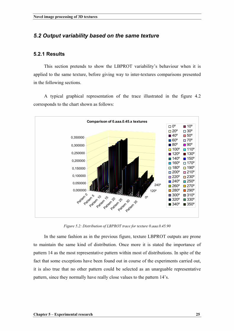
This section pretends to show the LBPROT variability’s behaviour when it is
applied to the same texture, before giving way to inter-textures comparisons presented
in the following sections.
A typical graphical representation of the trace illustrated in the figure 4.2
corresponds to the chart shown as follows:
Pattern
0
Pattern
5
Pattern
10
Pattern
15
Pattern
20
Pattern
25
Pattern
30
Pattern
350º
120º
240º0,000000
0,050000
0,100000
0,150000
0,200000
0,250000
0,300000
0,350000
Comparison of 0.aaa.0.45.x textures0º 10º20º 30º40º 50º60º 70º80º 90º100º 110º120º 130º140º 150º160º 170º180º 190º200º 210º220º 230º240º 250º260º 270º280º 290º300º 310º320º 330º340º 350º
Figure 5.2: Distribution of LBPROT trace for texture 0.aaa.0.45.90 In the same fashion as in the previous figure, texture LBPROT outputs are prone
to maintain the same kind of distribution. Once more it is stated the importance of
pattern 14 as the most representative pattern within most of distributions. In spite of the
fact that some exceptions have been found out in course of the experiments carried out,
it is also true that no other pattern could be selected as an unarguable representative
pattern, since they normally have really close values to the pattern 14’s.

Novel image processing of 3D textures
Chapter 5 – Experimental research 26
In order to find out in further detail the grade of the LBPROT variability before
same texture samples, another experiment was carried out consisting in selecting every
texture shown in figure 5.1 with slant angle valued to 45º and tilt to 90º. Afterwards,
four non-coincident samples with size 128 x 128 pixels each were obtained from those
textures. The starting points of the aforementioned four textures correspond to the
indicated as follows: section 1 upper-left corner, section 2 following 128 pixels after
section 1, section 3 next 128 beneath section 1, section 4 following 128 beneath section
2 and after section 3. Once the LBPROT texture operator was applied to them, the
following results were achieved graphically represented:
Figure 5.3: Variability of LBPROT for unidirectional textures with slant 45º and tilt 90º
Figure 5.4: Variability of LBPROT for bidirectional textures with slant 45º and tilt 90º
Behaviour 4 sections for pattern 14 in 1.acc.0.45.90
0500
1000150020002500
300035004000
45005000
Shift1 Shift2 Shift3 Shift4 Shift5 Shift6 Shift7 Shift8
Section1Section2Section3Section4
Behaviour 4 sections for pattern 14 in 1.adj.0.45.90
0
200
400
600
800
1000
1200
Shift1 Shift2 Shift3 Shift4 Shift5 Shift6 Shift7 Shift8
Section1Section2Section3Section4
Behaviour 4 sections for pattern 14 in 1.ach.0.45.90
0
1000
2000
3000
4000
5000
6000
Shift1 Shift2 Shift3 Shift4 Shift5 Shift6 Shift7 Shift8
Section1Section2Section3Section4
Behaviour 4 sections for pattern 14 in 1.afe.0.45.90
0
500
1000
1500
2000
2500
3000
Shift1 Shift2 Shift3 Shift4 Shift5 Shift6 Shift7 Shift8
Section1Section2Section3Section4

Novel image processing of 3D textures
Chapter 5 – Experimental research 27
Figure 5.5: Variability of LBPROT for multidirectional textures with slant 45º and tilt 90º
5.2.2 Assessments
To consider the pattern 14 as the most representative pattern seems to be feasible
for the reasons indicated above. Hence, it will be used as such for all experiments where
a single pattern has to be chosen.
On the other side, the most remarkable assessment at this point is the way in
which the LBPROT variability behaves. In that sense, it can be noted from figure 5.3
that it might present certain undesirable variability scenarios for unidirectional textures,
taking into account that all processed samples correspond to the same texture under
identical illumination conditions. In the same manner, the most enormous variability
example is illustrated in figure 5.4 where the bidirectional texture AFE obtains really
unequal results; observe how practically no point of the different waves matches.
However, the LBPROT variability is really tenuous on multidirectional texture, in
especial on AAR texture where classification results were excellent due to the really
close LBPROT’s behaviour for each section.
Behaviour 4 sections for pattern 14 in 1.aaa.0.45.90
0
500
1000
1500
2000
2500
3000
3500
4000
4500
Shift1 Shift2 Shift3 Shift4 Shift5 Shift6 Shift7 Shift8
Section1Section2Section3Section4
Behaviour 4 sections for pattern 14 in 1.aar.0.45.90
0
500
1000
1500
2000
2500
3000
3500
4000
4500
Shift1 Shift2 Shift3 Shift4 Shift5 Shift6 Shift7 Shift8
Section1Section2Section3Section4

Novel image processing of 3D textures
Chapter 5 – Experimental research 28
5.3 Investigation of unidirectional textures
5.3.1 Results
The aim of this point is to find out the behaviour of the LBPROT texture operator
under tilt illumination angle changes while keeping constant slant angle valued to 45º.
The table shown below is the result of putting together all pattern 14 rows of 12
different tilt angle images5 for ACC textures:
Table 5.1: Pattern 14 rows for 0.acc.0.45.x textures
When the values shown above are represented graphically, it is easier to
comprehend its meaning, and due to the large number of components to represent, they
have been depicted into two separate charts making clearer its visualization. A by rows
graphical representation is illustrated below:
Figure 5.6: Graphical behaviour of pattern 14 in 0.acc.0.45.x textures by rows
5 The term images might be used in this paper indistinctly to make reference to just textures.
Behaviour of pattern 14 in 0.acc.0.45.x images Grades/Shift Shift1 Shift2 Shift3 Shift4 Shift5 Shift6 Shift7 Shift8
0º 572 27050 23482 654 1077 34595 33743 89330º 1008 29398 19564 418 1428 42475 24692 116460º 2270 27450 12842 838 4492 32721 16705 254990º 4329 16921 7567 4775 8563 10831 11976 4705
120º 3988 14120 22416 6538 2024 10994 21252 3199150º 1962 22764 37955 1731 559 20366 24576 1498180º 1201 33441 34044 878 546 26465 23199 668210º 1440 41793 24682 1154 1017 28829 19647 464240º 4301 33221 16869 2396 2228 26866 13276 941270º 8092 10710 11822 4680 4221 16401 7512 4965300º 1699 11519 20703 3010 3587 14324 22852 6317330º 530 21295 24463 1266 1834 23409 38174 1517
05000
1000015000200002500030000350004000045000
Shift1 Shift2 Shift3 Shift4 Shift5 Shift6 Shift7 Shift8
0º
30º
60º
90º
120º
150º
05000
1000015000200002500030000350004000045000
Shift1 Shift2 Shift3 Shift4 Shift5 Shift6 Shift7 Shift8
180º
210º
240º
270º
300º
330º

Novel image processing of 3D textures
Chapter 5 – Experimental research 29
If the same process is followed6 again but using a 60º slant illumination angle
instead, the next results are achieved:
Figure 5.7: Graphical behaviour of pattern 14 in 0.acc.0.60.x textures by rows
Analogously, by changing the slant angle for 75º, the charts achieved are described below:
Figure 5.8: Graphical behaviour of pattern 14 in 0.acc.0.75.x textures by rows
The previous figures show high symmetry between pair of charts. Note how lines
with same colour and representing different tilt angles behave by describing a mirror
reflexion effect.
The following charts are obtained to represent exactly the same data than above
but by columns; a very useful radial representation accompanies each by-lines chart:
Figure 5.9: Graphical behaviour of pattern 14 in 0.acc.0.45.x textures by columns
6 In order to make this paper as clear as possible, most of tables with numerical values will be omitted from this point onwards. The reader might check the whole data by accessing to the appendix B.
0
10000
20000
30000
40000
50000
60000
Shift1 Shift2 Shift3 Shift4 Shift5 Shift6 Shift7 Shift8
0º
30º
60º
90º
120º
150º
0
10000
20000
30000
40000
50000
60000
Shift1 Shift2 Shift3 Shift4 Shift5 Shift6 Shift7 Shift8
180º
210º
240º
270º
300º
330º
0
10000
20000
30000
40000
50000
60000
Shift1 Shift2 Shift3 Shift4 Shift5 Shift6 Shift7 Shift8
0º
30º
60º
90º
120º
150º
0
10000
20000
30000
40000
50000
60000
Shift1 Shift2 Shift3 Shift4 Shift5 Shift6 Shift7 Shift8
180º
210º
240º
270º
300º
330º
Behaviour of pattern 14 in 0.acc.0.45.x images
05000
100001500020000250003000035000400004500050000
0º 30º
60º
90º
120º
150º
180º
210º
240º
270º
300º
330º
Shift1Shift2Shift3Shift4Shift5Shift6Shift7Shift8
Behaviour of pattern 14 in 0.acc.0.45.x images
0
10000
20000
30000
40000
500000º
30º
60º
90º
120º
150º
180º
210º
240º
270º
300º
330º
Shift1Shift2Shift3Shift4Shift5Shift6Shift7Shift8

Novel image processing of 3D textures
Chapter 5 – Experimental research 30
Figure 5.10: Graphical behaviour of pattern 14 in 0.acc.0.60.x textures by columns
Figure 5.11: Graphical behaviour of pattern 14 in 0.acc.0.75.x textures by columns The figures 5.9, 5.10 and 5.11 also have certain symmetrical behaviour, as by
using the division line formed by 270º and 90º in any radial chart as the border where to
bend it, each half-wave matches (mirror reflexion) with another different half-wave. For
instance the shift3 half-waves do it with the shift7 half-ones.
At this point the reader might have noted that there are enough cues as to think
that the symmetrical behaviour shown in the figures 5.6, 5.7 and 5.8 joined to the ones
shown in 5.9, 5.10 and 5.11 might lead us to synchronize somehow each wave with
another one. This aim can be achieved easily when every shift it is rotated -45º in they
same way as shown in the table for 0.acc.0.45.x texture below:
Behaviour of pattern 14 in 0.acc.0.60.x images
05000
100001500020000250003000035000400004500050000
0º 30º
60º
90º
120º
150º
180º
210º
240º
270º
300º
330º
Shift1Shift2Shift3Shift4Shift5Shift6Shift7Shift8
Behaviour of pattern 14 in 0.acc.0.60.x images
0
10000
20000
30000
40000
500000º
30º
60º
90º
120º
150º
180º
210º
240º
270º
300º
330º
Shift1Shift2Shift3Shift4Shift5Shift6Shift7Shift8
Behaviour of pattern 14 in 0.acc.0.75.x images
05000
100001500020000250003000035000400004500050000
0º 30º
60º
90º
120º
150º
180º
210º
240º
270º
300º
330º
Shift1Shift2Shift3Shift4Shift5Shift6Shift7Shift8
Behaviour of pattern 14 in 0.acc.0.75.x images
0
10000
20000
30000
40000
500000º
30º
60º
90º
120º
150º
180º
210º
240º
270º
300º
330º
Shift1Shift2Shift3Shift4Shift5Shift6Shift7Shift8

Novel image processing of 3D textures
Chapter 5 – Experimental research 31
Table 5.2: Behaviour of pattern 14 before 0.acc.0.45.x textures tilt angle shifts
The expected results are shown as follows:
Figure 5.12: Graphical behaviour of pattern 14 in 0.acc.0.45.x textures when synchronized by columns
Figure 5.13: Graphical behaviour of pattern 14 in 0.acc.0.60.x textures when synchronized by columns
Prediction table for 0.acc.0.45.x textures
Grades Shift1 Grades Shift2 Grades Shift3 Grades Shift4 Grades Shift5 Grades Shift6 Grades Shift7 Grades Shift80º 572 300º 11519 270º 11822 210º 1154 180º 546 120º 10994 90º 11976 30º 1164
30º 1008 330º 21295 300º 20703 240º 2396 210º 1017 150º 20366 120º 21252 60º 2549
60º 2270 0º 27050 330º 24463 270º 4680 240º 2228 180º 26465 150º 24576 90º 4705
90º 4329 30º 29398 0º 23482 300º 3010 270º 4221 210º 28829 180º 23199 120º 3199
120º 3988 60º 27450 30º 19564 330º 1266 300º 3587 240º 26866 210º 19647 150º 1498
150º 1962 90º 16921 60º 12842 0º 654 330º 1834 270º 16401 240º 13276 180º 668
180º 1201 120º 14120 90º 7567 30º 418 0º 1077 300º 14324 270º 7512 210º 464
210º 1440 150º 22764 120º 22416 60º 838 30º 1428 330º 23409 300º 22852 240º 941
240º 4301 180º 33441 150º 37955 90º 4775 60º 4492 0º 34595 330º 38174 270º 4965
270º 8092 210º 41793 180º 34044 120º 6538 90º 8563 30º 42475 0º 33743 300º 6317
300º 1699 240º 33221 210º 24682 150º 1731 120º 2024 60º 32721 30º 24692 330º 1517
330º 530 270º 10710 240º 16869 180º 878 150º 559 90º 10831 60º 16705 0º 893
Behaviour of shifts when moved -45º in 0.acc.0.45.x textures
0
5000
10000
15000
20000
25000
30000
35000
40000
45000
0º 30º 60º 90º 120º 150º 180º 210º 240º 270º 300º 330º
Shift1Shift2Shift3Shift4Shift5Shift6Shift7Shift8
Behaviour of shifts when moved -45º in 0.acc.0.45.x textures
0
10000
20000
30000
40000
500000º
30º
60º
90º
120º
150º
180º
210º
240º
270º
300º
330º
Shift1Shift2Shift3Shift4Shift5Shift6Shift7Shift8
Behaviour of shifts when moved -45º in 0.acc.0.60.x textures
0
10000
20000
30000
40000
50000
60000
0º 30º 60º 90º 120º 150º 180º 210º 240º 270º 300º 330º
Shif1Shif2Shif3Shif4Shif5Shif6Shif7Shif8
Behaviour of shifts when moved -45º in 0.acc.0.60.x textures
0
10000
20000
30000
40000
500000º
30º
60º
90º
120º
150º
180º
210º
240º
270º
300º
330º
Shif1Shif2Shif3Shif4Shif5Shif6Shif7Shif8
Novel image processing of 3D textures
Chapter 5 – Experimental research 32
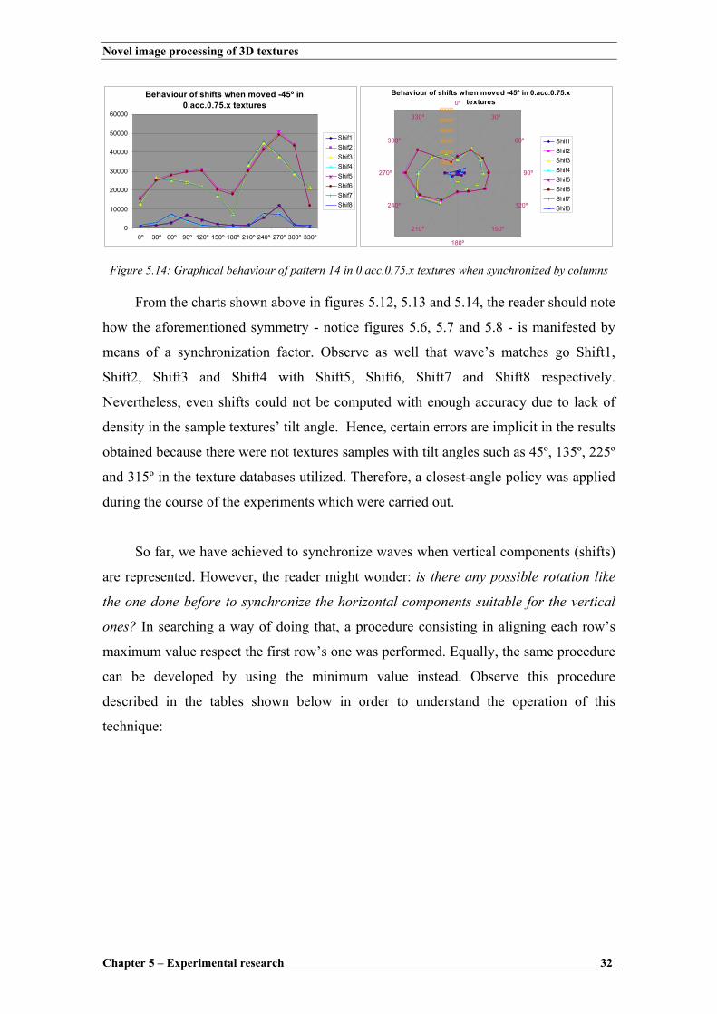
Figure 5.14: Graphical behaviour of pattern 14 in 0.acc.0.75.x textures when synchronized by columns
From the charts shown above in figures 5.12, 5.13 and 5.14, the reader should note
how the aforementioned symmetry - notice figures 5.6, 5.7 and 5.8 - is manifested by
means of a synchronization factor. Observe as well that wave’s matches go Shift1,
Shift2, Shift3 and Shift4 with Shift5, Shift6, Shift7 and Shift8 respectively.
Nevertheless, even shifts could not be computed with enough accuracy due to lack of
density in the sample textures’ tilt angle. Hence, certain errors are implicit in the results
obtained because there were not textures samples with tilt angles such as 45º, 135º, 225º
and 315º in the texture databases utilized. Therefore, a closest-angle policy was applied
during the course of the experiments which were carried out.
So far, we have achieved to synchronize waves when vertical components (shifts)
are represented. However, the reader might wonder: is there any possible rotation like
the one done before to synchronize the horizontal components suitable for the vertical
ones? In searching a way of doing that, a procedure consisting in aligning each row’s
maximum value respect the first row’s one was performed. Equally, the same procedure
can be developed by using the minimum value instead. Observe this procedure
described in the tables shown below in order to understand the operation of this
technique:
Behaviour of shifts when moved -45º in 0.acc.0.75.x textures
0
10000
20000
30000
40000
50000
60000
0º 30º 60º 90º 120º 150º 180º 210º 240º 270º 300º 330º
Shif1Shif2Shif3Shif4Shif5Shif6Shif7Shif8
Behaviour of shifts when moved -45º in 0.acc.0.75.x textures
0
10000
20000
30000
40000
50000
600000º
30º
60º
90º
120º
150º
180º
210º
240º
270º
300º
330º
Shif1Shif2Shif3Shif4Shif5Shif6Shif7Shif8

Novel image processing of 3D textures
Chapter 5 – Experimental research 33
Behaviour of pattern 14 in 0.acc.0.45.x textures MAX MIN
Grades/Shift Shift1 Shift2 Shift3 Shift4 Shift5 Shift6 Shift7 Shift8 0º 572 27050 23482 654 1077 34595 33743 893
30º 1008 29398 19564 418 1428 42475 24692 116460º 2270 27450 12842 838 4492 32721 16705 254990º 4329 16921 7567 4775 8563 10831 11976 4705120º 3988 14120 22416 6538 2024 10994 21252 3199150º 1962 22764 37955 1731 559 20366 24576 1498180º 1201 33441 34044 878 546 26465 23199 668210º 1440 41793 24682 1154 1017 28829 19647 464240º 4301 33221 16869 2396 2228 26866 13276 941270º 8092 10710 11822 4680 4221 16401 7512 4965300º 1699 11519 20703 3010 3587 14324 22852 6317330º 530 21295 24463 1266 1834 23409 38174 1517
Table 5.3: Maximum and minimum values for table5.1 (0.acc.0.45.x texture)
Table 5.4: Values of table 5.3 order by minimum value (0.acc.0.45.x texture)
Behaviour of pattern 14 placing min values in first column MAX MIN Grades/Shift Shift1 Shift2 Shift3 Shift4 Shift5 Shift6 Shift7 Shift8
0º 572 27050 23482 654 1077 34595 33743 893Grades/Shift Shift4 Shift5 Shift6 Shift7 Shift8 Shift1 Shift2 Shift3
30º 418 1428 42475 24692 1164 1008 29398 1956460º 838 4492 32721 16705 2549 2270 27450 12842
Grades/Shift Shift1 Shift2 Shift3 Shift4 Shift5 Shift6 Shift7 Shift8 90º 4329 16921 7567 4775 8563 10831 11976 4705
Grades/Shift Shift5 Shift6 Shift7 Shift8 Shift1 Shift2 Shift3 Shift4 120º 2024 10994 21252 3199 3988 14120 22416 6538150º 559 20366 24576 1498 1962 22764 37955 1731180º 546 26465 23199 668 1201 33441 34044 878
Grades/Shift Shift8 Shift1 Shift2 Shift3 Shift4 Shift5 Shift6 Shift7 210º 464 1440 41793 24682 1154 1017 28829 19647240º 941 4301 33221 16869 2396 2228 26866 13276
Grades/Shift Shift5 Shift6 Shift7 Shift8 Shift1 Shift2 Shift3 Shift4 270º 4221 16401 7512 4965 8092 10710 11822 4680
Grades/Shift Shift1 Shift2 Shift3 Shift4 Shift5 Shift6 Shift7 Shift8 300º 1699 11519 20703 3010 3587 14324 22852 6317330º 530 21295 24463 1266 1834 23409 38174 1517

Novel image processing of 3D textures
Chapter 5 – Experimental research 34
Figure 5.15: Graphical representation of table 5.3 order by minimum value (0.acc.0.45.x texture)
Behaviour of pattern 14 placing max values in sixth column MAX MIN Grades/Shift Shift1 Shift2 Shift3 Shift4 Shift5 Shift6 Shift7 Shift8
0º 572 27050 23482 654 1077 34595 33743 89330º 1008 29398 19564 418 1428 42475 24692 116460º 2270 27450 12842 838 4492 32721 16705 2549
Grades/Shift Shift5 Shift6 Shift7 Shift8 Shift1 Shift2 Shift3 Shift4 90º 8563 10831 11976 4705 4329 16921 7567 4775
Grades/Shift Shift6 Shift7 Shift8 Shift1 Shift2 Shift3 Shift4 Shift5 120º 10994 21252 3199 3988 14120 22416 6538 2024150º 20366 24576 1498 1962 22764 37955 1731 559180º 26465 23199 668 1201 33441 34044 878 546
Grades/Shift Shift5 Shift6 Shift7 Shift8 Shift1 Shift2 Shift3 Shift4 210º 1017 28829 19647 464 1440 41793 24682 1154240º 2228 26866 13276 941 4301 33221 16869 2396
Grades/Shift Shift1 Shift2 Shift3 Shift4 Shift5 Shift6 Shift7 Shift8 270º 8092 10710 11822 4680 4221 16401 7512 4965
Grades/Shift Shift2 Shift3 Shift4 Shift5 Shift6 Shift7 Shift8 Shift1 300º 11519 20703 3010 3587 14324 22852 6317 1699330º 21295 24463 1266 1834 23409 38174 1517 530
Table 5.5: Values of table 5.3 order by maximum value (0.acc.0.45.x texture)
Figure 5.16: Graphical representation of table 5.3 order by maximum value (0.acc.0.45.x texture)
0
5000
10000
15000
20000
25000
30000
35000
40000
45000
Shift1 Shift2 Shift3 Shift4 Shift5 Shift6 Shift7 Shift8
0º30º60º90º120º150º
0
5000
10000
15000
20000
25000
30000
35000
40000
45000
Shift1 Shift2 Shift3 Shift4 Shift5 Shift6 Shift7 Shift8
180º210º240º270º300º330º
0
5000
10000
15000
20000
25000
30000
35000
40000
45000
Shift1 Shift2 Shift3 Shift4 Shift5 Shift6 Shift7 Shift8
0º30º60º90º120º150º
0
5000
10000
15000
20000
25000
30000
35000
40000
45000
Shift1 Shift2 Shift3 Shift4 Shift5 Shift6 Shift7 Shift8
180º210º240º270º300º330º

Novel image processing of 3D textures
Chapter 5 – Experimental research 35
From the charts generated after applying this method, we can say that the
minimum values ordination works better than maximum values one, because whereas
the former keep the mentioned symmetry, the latter do not: compare the behaviour of 0º
and 180º waves to state this fact. Unfortunately, no spectacular improvement is gained
in our attempt of achieved a better horizontal components synchronization.
5.3.2 Assessments
The high symmetry achieved in figures 5.6, 5.7 and 5.8 would allow us to reduce
the computation loading needed to generate all those traces in a 50% when a good
approximation of the real values want to be obtained. However, when a texture such as
ADJ7 does not have the pattern 14 as the most representative value in many occasions,
the results obtained are not as good at the previously obtained with ACC texture. See
the following example:
Figure 5.17: Graphical behaviour of pattern 14 in 7.adj.0.45.x textures by rows
Although at first sight both charts seem to be quite close from each other, they
really are not when thoroughly analysed. Note for instance how 150º wave distances
from 330º in spite of initially it was expected to be quite close from each other
according to the previous experience. Nevertheless, certain symmetrical grade is
expected to obtain in all unidirectional traces which can be used, as mentioned in the
first paragraph of this section, to reduce computations expenses.
The reason why a great synchronization can be obtained in the charts shown in
figures 5.9, 5.10 and 5.11 by just doing -45º shifts seems to be due to the way in which
data is processed, that is, applying rotations on 8-bit size words. This allows no more
than 8 possible rotations, and hence 8 angles of 45º which all together encompass 360º. 7 A complete analysis of the ADJ texture is at the entire disposition of the reader in the appendix B, where more detailed information can be found.
0
5000
10000
15000
2000025000
30000
35000
40000
Shift1Shift2
Shift3Shift4
Shift5Shift6
Shift7Shift8
0º
30º
60º
90º
120º
150º0
5000
10000
1500020000
25000
30000
35000
40000
Shift1Shift2
Shift3
Shift4
Shift5
Shift6
Shift7
Shift8
180º
210º
240º
270º
300º
330º

Novel image processing of 3D textures
Chapter 5 – Experimental research 36
5.4 Investigation of bidirectional textures
5.4.1 Results
In this section we are dealing with bidirectional textures and we will see whether
the LBPROT texture operator behaves in the same way done so far or shows a different
conduct. Additionally, the same way of proceeding as in previous section is being
adopted along this one, showing just one example of bidirectional textures in high detail
and making mention of the most remarkable differences, if any, regarding the other
bidirectional texture studied thoroughly. Equally, no more tables will be shown what
will lead this section’s assessments to be derived from the charts8 illustrated below.
Therefore, the base texture traces for the pattern 14 are graphically represented in the
following three couple of charts:
Figure 5.18: Graphical behaviour of pattern 14 in 2.ach.0.45.x textures by rows
Figure 5.19: Graphical behaviour of pattern 14 in 2.ach.0.60.x textures by rows
8 The interested reader, who wants to know in further detail where all the following charts come from, might utilize the Appendix B where a detailed description of all these data and procedures are carefully presented.
0
5000
10000
15000
20000
25000
30000
Shift1 Shift2 Shif t3 Shif t4 Shif t5 Shif t6 Shift7 Shift8
0º
30º
60º
90º
120º
150º
0
5000
10000
15000
20000
25000
30000
Shift1 Shift2 Shift3 Shif t4 Shif t5 Shif t6 Shif t7 Shift8
180º
210º
240º
270º
300º
330º
0
5000
10000
15000
20000
25000
30000
Shift1 Shift2 Shif t3 Shif t4 Shif t5 Shif t6 Shift7 Shift8
0º
30º
60º
90º
120º
150º
0
5000
10000
15000
20000
25000
30000
Shift1 Shift2 Shift3 Shif t4 Shif t5 Shif t6 Shif t7 Shift8
180º
210º
240º
270º
300º
330º

Novel image processing of 3D textures
Chapter 5 – Experimental research 37
Figure 5.20: Graphical behaviour of pattern 14 in 2.ach.0.75.x textures by rows
The first remarkable characteristic derived from the three pairs of charts shown
above is that the grade of symmetry reached is not as good as we saw in the charts of
the previous section. In these charts (figures 5.18, 5.19 and 5.20) symmetry is just a
rough approximation. Like in the ACH bidirectional texture, the AFE texture shows an
irregular behaviour between pair of charts.
Another important feature the reader can note is how the changes in illumination
slant angle interfere in the peak values of each chart: the bigger the slant angle is, the
greater its peak values are. Notice how peak values of charts are closer to the upper
edge of their graphical representation, taking into account that all of them were
represented using the same scale.
In addition, not only the peak values change before variations in slant angle, but
also the shape of its weaves. For instance, observe the wave corresponding to 120º as
several changes can be perceived throughout those three figures.
Following the same line carried out so far along this paper, a by columns
graphical representations are illustrated below:
Figure 5.21: Graphical behaviour of pattern 14 in 2.ach.0.45.x textures by columns
0
5000
10000
15000
20000
25000
30000
Shift1 Shift2 Shif t3 Shif t4 Shif t5 Shif t6 Shift7 Shift8
0º
30º
60º
90º
120º
150º
0
5000
10000
15000
20000
25000
30000
Shift1 Shift2 Shift3 Shif t4 Shif t5 Shif t6 Shif t7 Shift8
180º
210º
240º
270º
300º
330º
Behaviour in 30º shifts for 2.ach.0.45.x images
0
5000
10000
15000
20000
25000
30000
35000
0º 30º
60º
90º
120º
150º
180º
210º
240º
270º
300º
330º
Shift1Shift2Shift3Shift4Shift5Shift6Shift7Shift8
Behaviour in 30º shifts for 2.ach.0.45.x images
0
5000
10000
15000
20000
25000
30000
350000º
30º
60º
90º
120º
150º
180º
210º
240º
270º
300º
330º
Shift1Shift2Shift3Shift4Shift5Shift6Shift7Shift8

Novel image processing of 3D textures
Chapter 5 – Experimental research 38
Figure 5.22: Graphical behaviour of pattern 14 in 2.ach.0.60.x textures by columns
Figure 5.23: Graphical behaviour of pattern 14 in 2.ach.0.75.x textures by columns
Same behaviour is once more shown in by columns charts; radial charts show
especially well this feature as it can be noted. Our aim at this point is then to try to
synchronize the wave in the best way possible. The results achieved are revealed in the
next graphical representations:
Figure 5.24: Graphical behaviour of pattern 14 in 2.ach.0.45.x textures when synchronized by columns
Behaviour in 30º shifts for 2.ach.0.60.x images
0
5000
10000
15000
20000
25000
30000
35000
0º 30º
60º
90º
120º
150º
180º
210º
240º
270º
300º
330º
Shift1Shift2Shift3Shift4Shift5Shift6Shift7Shift8
Behaviour in 30º shifts for 2.ach.0.60.x images
0
5000
10000
15000
20000
25000
30000
350000º
30º
60º
90º
120º
150º
180º
210º
240º
270º
300º
330º
Shift1Shift2Shift3Shift4Shift5Shift6Shift7Shift8
Behaviour in 30º shifts for 2.ach.0.75.x images
0
5000
10000
15000
20000
25000
30000
35000
0º 30º
60º
90º
120º
150º
180º
210º
240º
270º
300º
330º
Shift1Shift2Shift3Shift4Shift5Shift6Shift7Shift8
Behaviour in 30º shifts for 2.ach.0.75.x images
0
5000
10000
15000
20000
25000
30000
350000º
30º
60º
90º
120º
150º
180º
210º
240º
270º
300º
330º
Shift1Shift2Shift3Shift4Shift5Shift6Shift7Shift8
Behaviour of shifts when moved -45º in 2.ach.0.45.x textures
0
5000
10000
15000
20000
25000
30000
0º 30º 60º 90º 120º 150º 180º 210º 240º 270º 300º 330º
Shift1
Shift2
Shift3
Shift4
Shift5
Shift6
Shift7
Shift8
Behaviour of shifts when moved -45º in 2.ach.0.45.x textures
0
5000
10000
15000
20000
25000
300000º
30º
60º
90º
120º
150º
180º
210º
240º
270º
300º
330º
Shift1
Shift2
Shift3
Shift4
Shift5
Shift6
Shift7
Shift8

Novel image processing of 3D textures
Chapter 5 – Experimental research 39
Figure 5.25: Graphical behaviour of pattern 14 in 2.ach.0.60.x textures when synchronized by columns
Figure 5.26: Graphical behaviour of pattern 14 in 2.ach.0.75.x textures when synchronized by columns
All charts show an especially great adjustment within 0º and 150º section. In the
remaining range of grades, from 180º to 330º, the synchronization is divided into two
components. For one side all odd shifts keep all together, whereas for another all even
shifts carry out the same action. However, different synchronization results are obtained
from AFE counterpart. Let us show a brief example:
Figure 5.27: Graphical behaviour of pattern 14 in 6.afe.0.45/60.x textures when synchronized by columns
The same as in the previous section, an attempt to try to find out a by rows
synchronization was performed by using the same technique used there. In that manner,
Behaviour of shifts when moved -45º in 2.ach.0.60.x textures
0
5000
10000
15000
20000
25000
30000
0º 30º 60º 90º 120º 150º 180º 210º 240º 270º 300º 330º
Shift1
Shift2
Shift3
Shift4
Shift5
Shift6
Shift7
Shift8
Behaviour of shifts when moved -45º in 2.ach.0.60.x textures
0
5000
10000
15000
20000
25000
300000º
30º
60º
90º
120º
150º
180º
210º
240º
270º
300º
330º
Shift1
Shift2
Shift3
Shift4
Shift5
Shift6
Shift7
Shift8
Behaviour of shifts when moved -45º in 2.ach.0.75.x textures
0
5000
10000
15000
20000
25000
30000
0º 30º 60º 90º 120º 150º 180º 210º 240º 270º 300º 330º
Shift1
Shift2
Shift3
Shift4
Shift5
Shift6
Shift7
Shift8
Behaviour of shifts when moved -45º in 2.ach.0.75.x textures
0
5000
10000
15000
20000
25000
300000º
30º
60º
90º
120º
150º
180º
210º
240º
270º
300º
330º
Shift1
Shift2
Shift3
Shift4
Shift5
Shift6
Shift7
Shift8
Behaviour of shifts when moved -45º in 6.afe.0.45.x textures
0
5000
10000
15000
20000
25000
30000
0º 30º 60º 90º 120º 150º 180º 210º 240º 270º 300º 330º
Shift1Shift2Shift3Shift4Shift5Shift6Shift7Shift8
Behaviour of shifts when moved -45º in 6.afe.0.60.x textures
0
5000
10000
15000
20000
25000
30000
35000
0º 30º 60º 90º 120º 150º 180º 210º 240º 270º 300º 330º
Shift1Shift2Shift3Shift4Shift5Shift6Shift7Shift8
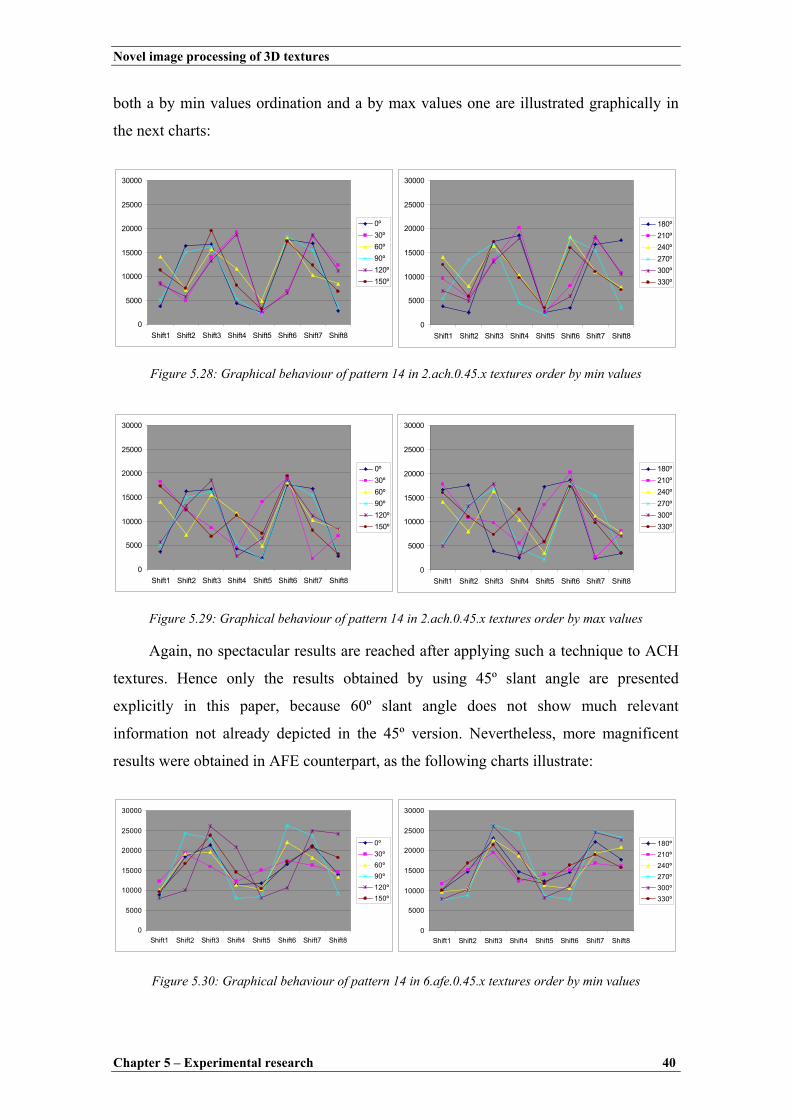
Novel image processing of 3D textures
Chapter 5 – Experimental research 40
both a by min values ordination and a by max values one are illustrated graphically in
the next charts:
Figure 5.28: Graphical behaviour of pattern 14 in 2.ach.0.45.x textures order by min values
Figure 5.29: Graphical behaviour of pattern 14 in 2.ach.0.45.x textures order by max values
Again, no spectacular results are reached after applying such a technique to ACH
textures. Hence only the results obtained by using 45º slant angle are presented
explicitly in this paper, because 60º slant angle does not show much relevant
information not already depicted in the 45º version. Nevertheless, more magnificent
results were obtained in AFE counterpart, as the following charts illustrate:
Figure 5.30: Graphical behaviour of pattern 14 in 6.afe.0.45.x textures order by min values
0
5000
10000
15000
20000
25000
30000
Shift1 Shift2 Shift3 Shift4 Shift5 Shift6 Shift7 Shift8
0º30º60º90º120º150º
0
5000
10000
15000
20000
25000
30000
Shift1 Shift2 Shift3 Shift4 Shift5 Shift6 Shift7 Shift8
180º210º240º270º300º330º
0
5000
10000
15000
20000
25000
30000
Shift1 Shift2 Shift3 Shift4 Shift5 Shift6 Shift7 Shift8
0º30º60º90º120º150º
0
5000
10000
15000
20000
25000
30000
Shift1 Shift2 Shift3 Shift4 Shift5 Shift6 Shift7 Shift8
180º210º240º270º300º330º
0
5000
10000
15000
20000
25000
30000
Shift1 Shift2 Shift3 Shift4 Shift5 Shift6 Shift7 Shift8
0º30º60º90º120º150º
0
5000
10000
15000
20000
25000
30000
Shift1 Shift2 Shift3 Shift4 Shift5 Shift6 Shift7 Shift8
180º210º240º270º300º330º

Novel image processing of 3D textures
Chapter 5 – Experimental research 41
Figure 5.31: Graphical behaviour of pattern 14 in 6.afe.0.45.x textures order by max values
Note how good the results obtained are for AFE texture, being especially good
where a by max values ordination were performed; the latter shows an almost perfect
symmetry.
5.4.2 Assessments
The first assessment is that a much closer synchronization is obtained in the
bidirectional texture than in the unidirectional ones (seen in the previous section), as
especially good results were achieved in charts shown in figures 5.24, 5.25 and 5.26.
This proximity throughout same texture traces lead us to think the possibility of
reaching certain computation saves once more. Effectively, up to a 75% computation
save can be achieved which allows a great deal of computing time reduction when
massive calculation is needed. Obviously, it cannot be expect to obtain high precision
values when traces are generated by this method, although it might be an excellent
solution for approximation problems.
0
5000
10000
15000
20000
25000
30000
Shift1 Shift2 Shift3 Shift4 Shift5 Shift6 Shift7 Shift8
0º30º60º90º120º150º
0
5000
10000
15000
20000
25000
30000
Shift1 Shift2 Shift3 Shift4 Shift5 Shift6 Shift7 Shift8
180º210º240º270º300º330º
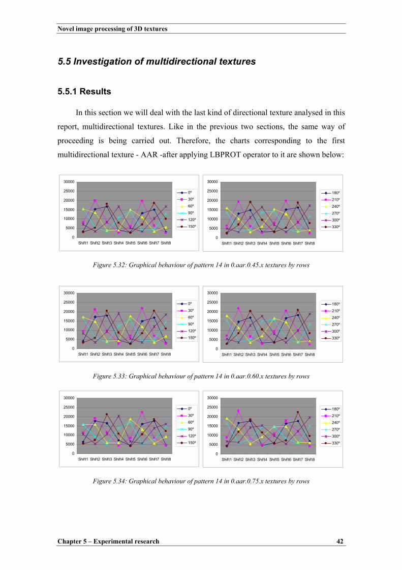
Novel image processing of 3D textures
Chapter 5 – Experimental research 42
5.5 Investigation of multidirectional textures
5.5.1 Results
In this section we will deal with the last kind of directional texture analysed in this
report, multidirectional textures. Like in the previous two sections, the same way of
proceeding is being carried out. Therefore, the charts corresponding to the first
multidirectional texture - AAR -after applying LBPROT operator to it are shown below:
Figure 5.32: Graphical behaviour of pattern 14 in 0.aar.0.45.x textures by rows
Figure 5.33: Graphical behaviour of pattern 14 in 0.aar.0.60.x textures by rows
Figure 5.34: Graphical behaviour of pattern 14 in 0.aar.0.75.x textures by rows
0
5000
10000
15000
20000
25000
30000
Shift1 Shift2 Shift3 Shift4 Shif t5 Shif t6 Shif t7 Shift8
0º
30º
60º
90º
120º
150º
0
5000
10000
15000
20000
25000
30000
Shift1 Shif t2 Shif t3 Shift4 Shift5 Shift6 Shift7 Shift8
180º
210º
240º
270º
300º
330º
0
5000
10000
15000
20000
25000
30000
Shift1 Shift2 Shift3 Shift4 Shif t5 Shif t6 Shif t7 Shift8
0º
30º
60º
90º
120º
150º
0
5000
10000
15000
20000
25000
30000
Shift1 Shif t2 Shif t3 Shift4 Shift5 Shift6 Shift7 Shift8
180º
210º
240º
270º
300º
330º
0
5000
10000
15000
20000
25000
30000
Shift1 Shift2 Shift3 Shift4 Shif t5 Shif t6 Shif t7 Shift8
0º
30º
60º
90º
120º
150º
0
5000
10000
15000
20000
25000
30000
Shift1 Shif t2 Shif t3 Shift4 Shift5 Shift6 Shift7 Shift8
180º
210º
240º
270º
300º
330º

Novel image processing of 3D textures
Chapter 5 – Experimental research 43
Broadly speaking, results from multidirectional texture are prone to be more
regular and uniform than the ones from unidirectional and bidirectional texture,
independently of the operator used. Like the experimented reader might have guessed,
such behaviour is effectively present in the results achieved for the multidirectional
texture AAR by using 45º, 60º and 75º slant angles, as figures 5.32, 5.33 and 5.34
clearly show above. In that sense, although at the first sight it might not be so
perceptible, each chart is symmetrical to its neighbour from the same pair it belongs to.
However, figure 5.34 deserves especial attention because the symmetry detected does
not evolve in the same manner that figures 5.32 and 5.33 did. Observe that if the waves
from 180º to 330º are moved one shift to the right following a cycle, the same grade of
symmetry comes up for this figure as well.
Once more, changes in illumination slant angle produce variations in peak values
generated for the LBPROT texture operator. However, note that these variations are not
enormous under small changes of slant angle what gives certain uniform behaviour to
the LBPROT.
The following charts represent the data seen in previous charts but by columns
disposition instead:
Figure 5.35: Graphical behaviour of pattern 14 in 0.aar.0.45.x textures by columns
Behaviour in 30º shifts for 0.aar.0.45.x images
0
5000
10000
15000
20000
25000
30000
35000
0º 30º
60º
90º
120º
150º
180º
210º
240º
270º
300º
330º
Shift1Shift2Shift3Shift4Shift5Shift6Shift7Shift8
Behaviour in 30º shifts for 0.aar.0.45.x images
0
5000
10000
15000
20000
25000
30000
350000º
30º
60º
90º
120º
150º
180º
210º
240º
270º
300º
330º
Shift1Shift2Shift3Shift4Shift5Shift6Shift7Shift8
Behaviour in 30º shifts for 0.aar.0.60.x images
0
5000
10000
15000
20000
25000
30000
35000
0º 30º
60º
90º
120º
150º
180º
210º
240º
270º
300º
330º
Shift1Shift2Shift3Shift4Shift5Shift6Shift7Shift8
Behaviour in 30º shifts for 0.aar.0.60.x images
0
5000
10000
15000
20000
25000
30000
350000º
30º
60º
90º
120º
150º
180º
210º
240º
270º
300º
330º
Shift1Shift2Shift3Shift4Shift5Shift6Shift7Shift8

Novel image processing of 3D textures
Chapter 5 – Experimental research 44
Figure 5.36: Graphical behaviour of pattern 14 in 0.aar.0.60.x textures by columns
Figure 5.37: Graphical behaviour of pattern 14 in 0.aar.0.75.x textures by columns
From the previous three figures it can be inferred a great symmetry, even bigger
than the one achieved in all previous experiments. Such grade of symmetry lead to an
amazing synchronization as can be observed in the following figures:
Figure 5.38: Graphical behaviour of pattern 14 in 0.aar.0.45.x textures when synchronized by columns
Figure 5.39: Graphical behaviour of pattern 14 in 0.aar.0.60.x textures when synchronized by columns
Behaviour in 30º shifts for 0.aar.0.75.x images
0
5000
10000
15000
20000
25000
30000
35000
0º 30º
60º
90º
120º
150º
180º
210º
240º
270º
300º
330º
Shift1Shift2Shift3Shift4Shift5Shift6Shift7Shift8
Behaviour in 30º shifts for 0.aar.0.75.x images
0
5000
10000
15000
20000
25000
30000
350000º
30º
60º
90º
120º
150º
180º
210º
240º
270º
300º
330º
Shift1Shift2Shift3Shift4Shift5Shift6Shift7Shift8
Behaviour of shifts when moved -45º in 0.aar.0.45.x textures
0
5000
10000
15000
20000
25000
30000
0º 30º 60º 90º 120º 150º 180º 210º 240º 270º 300º 330º
Shift1
Shift2
Shift3
Shift4
Shift5
Shift6
Shift7
Shift8
Behaviour of shifts when moved -45º in 0.aar.0.45.x textures
0
5000
10000
15000
20000
25000
300000º
30º
60º
90º
120º
150º
180º
210º
240º
270º
300º
330º
Shift1
Shift2
Shift3
Shift4
Shift5
Shift6
Shift7
Shift8
Behaviour of shifts when moved -45º in 0.aar.0.60.x textures
0
5000
10000
15000
20000
25000
30000
0º 30º 60º 90º 120º 150º 180º 210º 240º 270º 300º 330º
Shift1
Shift2
Shift3
Shift4
Shift5
Shift6
Shift7
Shift8
Behaviour of shifts when moved -45º in 0.aar.0.60.x textures
0
5000
10000
15000
20000
25000
300000º
30º
60º
90º
120º
150º
180º
210º
240º
270º
300º
330º
Shift1
Shift2
Shift3
Shift4
Shift5
Shift6
Shift7
Shift8

Novel image processing of 3D textures
Chapter 5 – Experimental research 45
Figure 5.40: Graphical behaviour of pattern 14 in 0.aar.0.75.x textures when synchronized by columns
As aforementioned, the proximity of the waves of figures 5.38, 5.39 and 5.40
show the same behaviour and a really weak variation under slant angle changes. In the
same manner, similar results were obtained from the experiments carried out with AAA
texture, taking into account that this texture could be studied in higher detail than the
rest due to the availability of a denser repertory of samples, which varied in steps of 10º.
Consequently, let us illustrate these comments briefly with a couple of charts derived
from its experiments:
Figure 5.41: Graphical behaviour of pattern 14 in 0.aaa.0.45/75.x textures when synchronized by columns
Behaviour of shifts when moved -45º in 0.aar.0.75.x textures
0
5000
10000
15000
20000
25000
30000
0º 30º 60º 90º 120º 150º 180º 210º 240º 270º 300º 330º
Shift1
Shift2
Shift3
Shift4
Shift5
Shift6
Shift7
Shift8
Behaviour of shifts when moved -45º in 0.aar.0.75.x textures
0
5000
10000
15000
20000
25000
300000º
30º
60º
90º
120º
150º
180º
210º
240º
270º
300º
330º
Shift1
Shift2
Shift3
Shift4
Shift5
Shift6
Shift7
Shift8
Behaviour of shifts when moved -45º in 0.aaa.0.45.x textures
0
5000
10000
15000
20000
25000
0º 30º
60º
90º
120º
150º
180º
210º
240º
270º
300º
330º
Shift1Shift2Shift3Shift4Shift5Shift6Shift7Shift8
Behaviour of shifts when moved -45º in 0.aaa.0.75.x textures
0
5000
10000
15000
20000
25000
0º 20º
40º
60º
80º
100º
120º
140º
160º
180º
200º
220º
240º
260º
280º
300º
320º
340º
Shift1Shift2Shift3Shift4Shift5Shift6Shift7Shift8

Novel image processing of 3D textures
Chapter 5 – Experimental research 46
Finally, in our already usual attempt to try to synchronize waves horizontally, the
charts shown in figure 5.42 and 5.43 below were the results reached:
Figure 5.42: Graphical behaviour of pattern 14 in 0.aar.0.45.x textures order by min values
Figure 5.43: Graphical behaviour of pattern 14 in 0.aar.0.45.x textures order by max values
Observe the great symmetry achieved in these charts on both by max and by min
ordination graphical representations what demonstrate a great rotation-invariant feature.
5.5.2 Assessments
The symmetry observed in this section between pairs of charts of each figure
added to the one within each chart per se, it allows to reduce the computation costs in
up to 75% to obtain good approximation traces with low calculation expenses.
Another remarkable aspect which deserves to be commented is the high symmetry
obtained throughout LBPROT experiments performed in this section: figure 5.41 is an
outstanding example of this characteristic.
0
5000
10000
15000
20000
25000
30000
Shift1 Shift2 Shift3 Shift4 Shift5 Shift6 Shift7 Shift8
0º30º60º90º120º150º
0
5000
10000
15000
20000
25000
30000
Shift1 Shift2 Shift3 Shift4 Shift5 Shift6 Shift7 Shift8
180º210º240º270º300º330º
0
5000
10000
15000
20000
25000
30000
Shift1 Shift2 Shift3 Shift4 Shift5 Shift6 Shift7 Shift8
0º30º60º90º120º150º
0
5000
10000
15000
20000
25000
30000
Shift1 Shift2 Shift3 Shift4 Shift5 Shift6 Shift7 Shift8
180º210º240º270º300º330º

Novel image processing of 3D textures
Chapter 5 – Experimental research 47
5.6 G statistic experiments
5.6.1 Results In this section we will deal with the usage of G statistic as a classifier based on
LBPROT outputs9. The same way of proceeding used so far is being adopted to develop
the experiments illustrated later. Therefore, the textures AAA, AAR, ACC, ACH, AFE
and ADJ presented in figure 5.1 have been used due to their directionality properties.
From all texture, four parts sized 128 x 128 pixels were obtained in the way already
described in the second section of this chapter. By using these textures, a table
containing the Cartesian product of all samples is then created. The values dispose by
columns represent the samples, whereas the rest are the models. For instance, the table
shown below corresponds with the piece of such a table where AAA texture is used as
model distribution and the rest of textures are samples (in left column):
Table 5.6: G statistic results for four parts of AAA texture
9 More information about how to perform such a task was explained in the chapter number 4 section 2.
0.aaa.0.45.90.part01 0.aaa.0.45.90.part02 0.aaa.0.45.90.part03 0.aaa.0.45.90.part04 0.aaa.0.45.90.part01 nan nan nan nan 0.aaa.0.45.90.part02 nan 0,000000 0,000346 0,0004780.aaa.0.45.90.part03 nan 0,000346 0,000001 0,0001950.aaa.0.45.90.part04 nan 0,000478 0,000195 0,0000000.aar.0.45.90.part01 nan 0,002127 0,002155 0,0025890.aar.0.45.90.part02 nan 0,002716 0,002827 0,0033100.aar.0.45.90.part03 nan 0,001779 0,001873 0,0022550.aar.0.45.90.part04 nan 0,002035 0,002082 0,0025071.acc.0.45.90.part01 nan 0,003504 0,002540 0,0026231.acc.0.45.90.part02 nan 0,008226 0,007097 0,0073591.acc.0.45.90.part03 nan 0,002320 0,001714 0,0019491.acc.0.45.90.part04 nan 0,003533 0,002591 0,0026892.ach.0.45.90.part01 nan 0,008678 0,009169 0,0089162.ach.0.45.90.part02 nan 0,005820 0,006020 0,0058162.ach.0.45.90.part03 nan 0,006281 0,005990 0,0056742.ach.0.45.90.part04 nan 0,005430 0,005143 0,0048506.afe.0.45.90.part01 nan 0,130903 0,125743 0,1256296.afe.0.45.90.part02 nan 0,079292 0,075113 0,0751776.afe.0.45.90.part03 nan 0,157789 0,152246 0,1522116.afe.0.45.90.part04 nan 0,216506 0,210103 0,2100297.adj.0.45.90.part01 nan 0,306070 0,298942 0,2988527.adj.0.45.90.part02 nan 0,346063 0,338778 0,3387207.adj.0.45.90.part03 nan 0,259126 0,252466 0,2524327.adj.0.45.90.part04 nan 0,340733 0,333447 0,333364

Novel image processing of 3D textures
Chapter 5 – Experimental research 48
The first remarkable feature which catches the reader attention is the sequence of
nan values spread throughout the previous table. The program coded to carried out this
calculations is based on the formula (5) seen in the previous chapter. When in a given
input texture there is at least one pattern which frequency – times it occurs for a given
texture – is equal to zero, the logarithm needed there cannot be calculated what it
generates an internal exception transformed into Non-A-Number (nan) value.
Moreover, the shadowed section of the table is the result of same texture outputs
and the diagonal corresponds to exactly the same part. The latter’s theoretical value
should be zero, although due to round errors some extra decimals might be introduced.
The rest of the aforementioned Cartesian table will not be presented in this
chapter, but the reader might analyse it thoroughly by accessing to the Appendix B.
Therefore, only their graphical representations will be illustrated throughout this
section. They are depicted as follows:
Figure 5.44: G statistic behaviour for unidirectional textures used as samples
0,0000000,0500000,1000000,1500000,2000000,2500000,3000000,3500000,4000000,450000
0.aaa
.0.45
.90.part
01
0.aaa
.0.45
.90.part
04
0.aar.
0.45.9
0.part
03
1.acc
.0.45.90
.part0
2
2.ach
.0.45
.90.pa
rt01
2.ach
.0.45
.90.pa
rt04
6.afe.0.
45.90
.part03
7.adj.
0.45.9
0.part
02
7.adj.0.45.90.part017.adj.0.45.90.part027.adj.0.45.90.part037.adj.0.45.90.part04
0,0000000,0500000,1000000,1500000,2000000,2500000,3000000,3500000,4000000,450000
0.aaa
.0.45
.90.part
01
0.aaa
.0.45
.90.part
04
0.aar.
0.45.9
0.part
03
1.acc
.0.45.90
.part0
2
2.ach
.0.45
.90.pa
rt01
2.ach
.0.45
.90.pa
rt04
6.afe.0.
45.90
.part03
7.adj.
0.45.9
0.part
02
1.acc.0.45.90.part01
1.acc.0.45.90.part02
1.acc.0.45.90.part03
1.acc.0.45.90.part04

Novel image processing of 3D textures
Chapter 5 – Experimental research 49
Figure 5.45: G statistic behaviour for bidirectional textures used as samples
Figure 5.46: G statistic behaviour for multidirectional textures used as samples
5.6.2 Assessments G statistic cannot be used on texture where at least one pattern does not occur.
This is especially likely as decreasing the size of the texture to be treated, what makes it
inappropriate for those particular cases. In those occasions where any pattern does not
occur, a frustrating nan value will be outputted, making impossible to obtain any
conclusion at all.
0,0000000,0500000,1000000,1500000,2000000,2500000,3000000,3500000,4000000,450000
0.aaa
.0.45
.90.part
01
0.aaa
.0.45
.90.part
04
0.aar.
0.45.9
0.part
03
1.acc
.0.45.90
.part0
2
2.ach
.0.45
.90.pa
rt01
2.ach
.0.45
.90.pa
rt04
6.afe.0.
45.90
.part03
7.adj.
0.45.9
0.part
02
0.aar.0.45.90.part01
0.aar.0.45.90.part02
0.aar.0.45.90.part03
0.aar.0.45.90.part04
0,0000000,0500000,1000000,1500000,2000000,2500000,3000000,3500000,4000000,450000
0.aaa
.0.45
.90.part
01
0.aaa
.0.45
.90.part
04
0.aar.
0.45.9
0.part
03
1.acc
.0.45.90
.part0
2
2.ach
.0.45
.90.pa
rt01
2.ach
.0.45
.90.pa
rt04
6.afe.0.
45.90
.part03
7.adj.
0.45.9
0.part
02
0.aaa.0.45.90.part01
0.aaa.0.45.90.part02
0.aaa.0.45.90.part03
0.aaa.0.45.90.part04
0,0000000,0500000,1000000,1500000,2000000,2500000,3000000,3500000,4000000,450000
0.aaa
.0.45
.90.part
01
0.aaa
.0.45
.90.part
04
0.aar.
0.45.9
0.part
03
1.acc
.0.45.90
.part0
2
2.ach
.0.45
.90.pa
rt01
2.ach
.0.45
.90.pa
rt04
6.afe.0.
45.90
.part03
7.adj.
0.45.9
0.part
02
2.ach.0.45.90.part01
2.ach.0.45.90.part02
2.ach.0.45.90.part03
2.ach.0.45.90.part04
0,0000000,0500000,1000000,1500000,2000000,2500000,3000000,3500000,4000000,450000
0.aaa
.0.45
.90.part
01
0.aaa
.0.45
.90.part
04
0.aar.
0.45.9
0.part
03
1.acc
.0.45.90
.part0
2
2.ach
.0.45
.90.pa
rt01
2.ach
.0.45
.90.pa
rt04
6.afe.0.
45.90
.part03
7.adj.
0.45.9
0.part
02
6.afe.0.45.90.part016.afe.0.45.90.part026.afe.0.45.90.part036.afe.0.45.90.part04

Novel image processing of 3D textures
Chapter 5 – Experimental research 50
Furthermore, observe how classification in figures 5.44, 5.45 and 5.46 evolve, as
ACC, ACH, AAA and AAR have really close values from each other, providing hence a
really weak discrimination features. Although AFE texture provides slightly better
classification results, they are not good enough either, as absolutely different textures -
such as ACH and ADJ - have close values particularly for part 2. Nevertheless, the best
classification results were obtained by using ADJ texture as model because more variety
is manifested along each wave, providing consequently the highest discrimination
features among the tested texture.
Finally, observe that in spite of using the same texture as model in each chart, an
important variability is detected from the usage of one part of a particular texture to
another. Such behaviour is especially outstanding in texture ADJ and AFE shown
previously in figures 5.44 and 5.45 respectively. This factor should be taken into
account when classifying if a set of regular outputs is intended to obtain. Additionally,
such variability darkens the good discriminating features commented in the previous
paragraph, as it attenuates uniformness in the behaviour of those textures when they are
used as models.

Novel image processing of 3D textures
Chapter 6 – Conclusions 51
Chapter 6 – Conclusions LBPROT has showed some of its virtues along this paper like an excellent
behaviour before changes in tilt angle. This desirable feature is reachable in greater
grade as closer multidirectional feature a texture owns. Nonetheless, good results were
obtained in all kind of textures, although - like in many other investigations -
multidirectional textures are more easily classifiable; figures 5.15, 5.16, 5.30, 5.31, 5.42
and 5.43 have stated these facts.
The operator has a good response to variations in slant angle, as comparing the
charts associated to a given texture under identical conditions but slant angle, the effect
achieved is that all charts are a stretched or shrunken versions one from another. By
simply using any normalization technique, spectacular results might be achieved in this
sense.

Novel image processing of 3D textures
Chapter 7 – Future work 52
Chapter 7 – Future work
Due to the fact that only three slant angles were managed along this project: 45º,
60º and 75º, a more thoroughly study should be performed in order to state the real
behaviour of LBPROT texture operator before slant angle changes. An important
limitation has bound the development of this project avoiding further results to be
obtained. We refer to all experiments in which rotation multiple of 45º were performed,
as they could not be carried out with the precision initially expected, due to the lack of
density in the tilt angle in the texture database used.
Moreover, further results are expected from this operator, as some illumination
prediction might be achievable by basing upon the experiments presented in this paper.
Little results were achieved in this line, but hopes on it seem to be reasonable.

Novel image processing of 3D textures
References 53
References [1] ROTATION-INVARIANT TEXTURE CLASSIFICATION USING FEATURE DISTRIBUTIONS M. PIETIKÄINEN, T. OJALA and Z. XU Machine Vision and Media Processing Group, Infotech Oulu University of Oulu, P.O. Box 4500 , FIN-90401 Oulu, Finlan www.mediateam.oulu.fi/publications/pdf/7.pdf - 18 Ago 2003 [2] H. Choi and R. G. Baraniuk, Multiscale image segmentation using wavelet-domain hidden Markov models, IEEE Transactions on Image Processing, 10 (September 2001): 1309-1321. http://www-dsp.rice.edu/publicationsold/pub/choi99mu.pdf [3] Rotation-Invariant Texture Classification Using a Complete Space-Frequency Model George M. Haley and B. S. Manjunath (1999), Member, IEEE. http://citeseer.nj.nec.com/cache/papers/cs/18678/http:zSzzSzverdi.ece.ucsb.eduzSzpublicationszSz99IPTrans.pdf/haley99rotationinvariant.pdf [4] H. Greenspan, S. Belongie, P. Perona and R. Goodman, Rotation Invariant Texture Recognition Using a Steerable Pyramid ICPR 1994, Jerusalem, Israel, pp. 162-7 vol 2. http://www.eng.tau.ac.il/~hayit/publications/ICPR94-texture.ps.Z [5] P. P. Raghu and B. Yegnanarayana, Senior Member, IEEE Supervised Texture Classification Using a Probabilistic Neural Network and Constraint Satisfaction Model http://speech.cs.iitm.ernet.in/~yegna/Publications/J04.pdf [6] Song-Yee Yoon, A robust neural network texture classifier, Term paper for 9.520 Department of Brain and Cognitive Sciences, MIT June 1997 http://www-bcs.mit.edu/~songyee/scale.html

Novel image processing of 3D textures
Appendix A: Source code 54
Appendix A: Source code
The following code demonstrates the uniqueness of the 36 rotation-invariant patterns for 8-bits size words:
File: test.cpp
#include <stdio.h> #include <stdlib.h> # define SIZE 64 # define WINSIZE 3 /* 36 possible LBPROT patterns: 00000000 -> 0xOO 00000001 -> 0x01 00000011 -> 0x03 00000101 -> 0x05 00001001 -> 0x09 00010001 -> 0x11 00000111 -> 0x07 00001011 -> 0x0B 00010011 -> 0x13 00100011 -> 0x23 01000011 -> 0x43 00010101 -> 0x15 00100101 -> 0x25 00001111 -> 0x0F 00010111 -> 0x17

Novel image processing of 3D textures
Appendix A: Source code 55
00100111 -> 0x27 01000111 -> 0x47 00011011 -> 0x1B 00110011 -> 0x33 01010101 -> 0x55 01010011 -> 0x53 01010110 -> 0x56 01001011 -> 0x4B 00011111 -> 0x1F 00101111 -> 0x2F 01001111 -> 0x4F 00110111 -> 0x37 01100111 -> 0x67 01010111 -> 0x57 01011011 -> 0x5B 00111111 -> 0x3F 01011111 -> 0x5F 01101111 -> 0x6F 01110111 -> 0x77 01111111 -> 0x7F 11111111 -> 0xFF */ /* First version const unsigned char Pattern[36]={0x00, 0x01, 0x03, 0x05, 0x09, 0x11, 0x07, 0x0B, 0x13, 0x23, 0x43, 0x15, 0x25, 0x45, 0x0F, 0x17, 0x27, 0x47, 0x1B, 0x33, 0x63, 0x55, 0x53, 0x56, 0x1F, 0x2F, 0x4F, 0x37, 0x67, 0x57, 0x3F, 0x5F, 0x6F, 0x77, 0x7F, 0xFF}; */ //Refined version const unsigned char Pattern[36]={0x00, 0x01, 0x03, 0x05, 0x09, 0x11,

Novel image processing of 3D textures
Appendix A: Source code 56
0x07, 0x0B, 0x13, 0x23, 0x43, 0x15, 0x25, 0x4B, 0x0F, 0x17, 0x27, 0x47, 0x1B, 0x33, 0x55, 0x53, 0x56, 0x1F, 0x2F, 0x4F, 0x37, 0x67, 0x57, 0x5B, 0x3F, 0x5F, 0x6F, 0x77, 0x7F, 0xFF}; int main() { for (int j=0; j<256; j++) { unsigned char count = 0; unsigned char tmp = j; bool found = false; // Demonstrate there is an equivalent pattern for every number while (!found) { if (count++ == 8) { printf("There is no equivalent Pattern for value %d\n", j); break; } for (int k=0; k < 36; k++) { //if (j == k) continue; if (Pattern[k] == tmp) { found = true; //printf("Pattern %d is equivalent to Pattern %d\n", j, k); break; } } /* if (j == 0) printf("Iter-> %d; K-> %d: K1-> %d + K2-> %d = K3-> %d\n", count, tmp, (tmp<<1)&255, tmp>>7, ((tmp<<1)&255 | (tmp>>7)) ); */

Novel image processing of 3D textures
Appendix A: Source code 57
tmp = (tmp<<1)&255 | (tmp >> 7); } // Demonstrate there are not equivalent each other tmp = Pattern[j]; count = 0; if (j <36) while (count++ < 8) { for (int k=0; k < 36; k++) { if (j == k) continue; if (Pattern[k] == tmp) { printf("Pattern %d is equivalent to Pattern %d\n", j, k); break; } } tmp = (tmp<<1)&255 | (tmp >> 7); } } printf("Finish!\n"); }

Novel image processing of 3D textures
Appendix A: Source code 58
The next code corresponds to the LBPROT implementation used in this project based on SCOPE format texture files.
File: LBPROT.cpp /* * NAME * LBPROT.cpp * SYNOPSIS * Function: unsigned char * LBPROT(float *matrix, int height = SIZE, int width = SIZE); * AUTHOR * Carlos Lopez Sanchez * MODIFICATION * * MODULES REQUIRED * libscope.a */ /* #ifdef __cplusplus extern "C" { #endif // declarations #include "./scope-src/scope.h" #include "./scope-src/image_if2.h" #include <stdio.h> #include <stdlib.h> #include <string.h> #include <math.h> #ifdef __cplusplus } #endif

Novel image processing of 3D textures
Appendix A: Source code 59
*/ #include <stdio.h> #include <stdlib.h> #include <string.h> #include <math.h> #include "./scope-src/scope.h" #include "./scope-src/image_if2.h" # define SIZE 64 # define WINSIZE 3 # define BINS 36 // Number of bins /* 36 possible LBPROT patterns: 00000000 -> 0xOO 00000001 -> 0x01 00000011 -> 0x03 00000101 -> 0x05 00001001 -> 0x09 00010001 -> 0x11 00000111 -> 0x07 00001011 -> 0x0B 00010011 -> 0x13 00100011 -> 0x23 01000011 -> 0x43 00010101 -> 0x15 00100101 -> 0x25 00001111 -> 0x0F 00010111 -> 0x17 00100111 -> 0x27
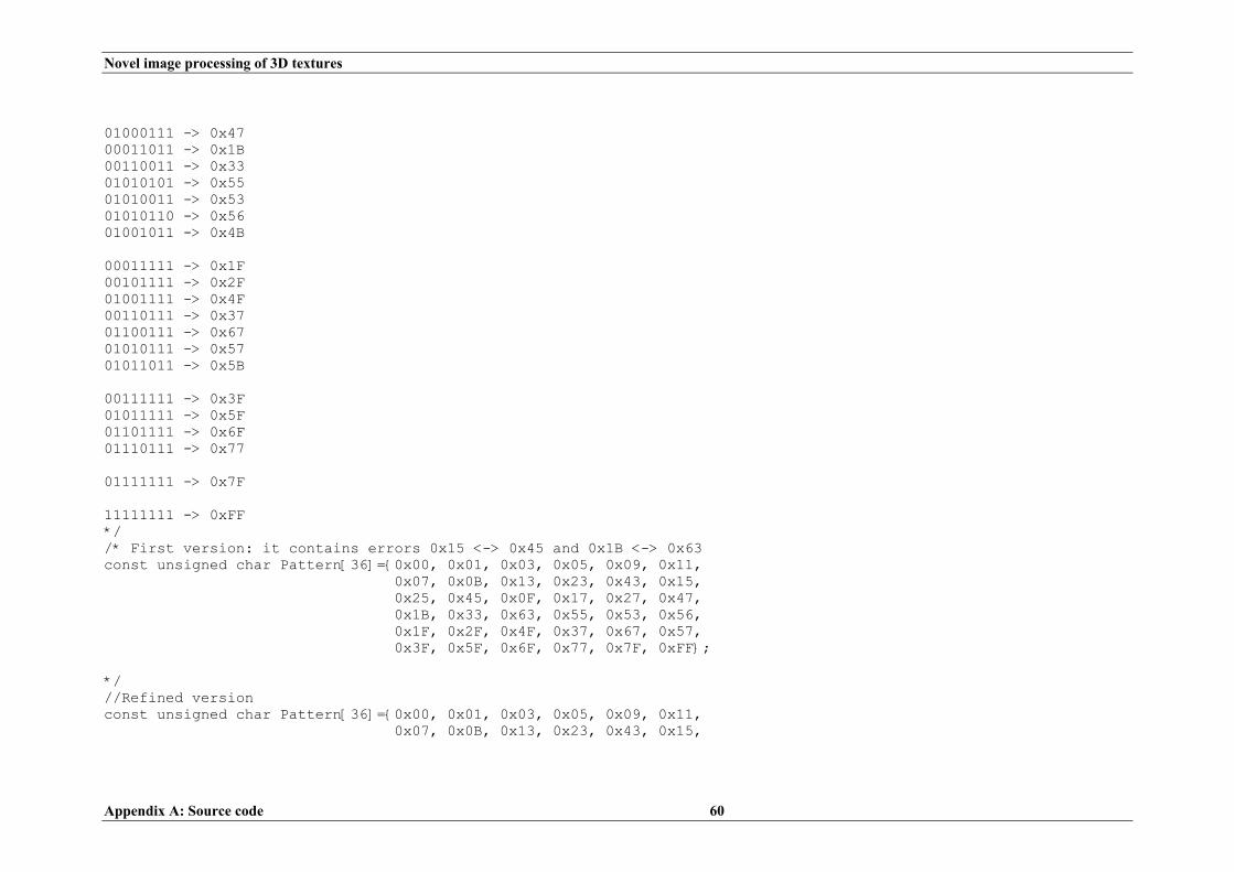
Novel image processing of 3D textures
Appendix A: Source code 60
01000111 -> 0x47 00011011 -> 0x1B 00110011 -> 0x33 01010101 -> 0x55 01010011 -> 0x53 01010110 -> 0x56 01001011 -> 0x4B 00011111 -> 0x1F 00101111 -> 0x2F 01001111 -> 0x4F 00110111 -> 0x37 01100111 -> 0x67 01010111 -> 0x57 01011011 -> 0x5B 00111111 -> 0x3F 01011111 -> 0x5F 01101111 -> 0x6F 01110111 -> 0x77 01111111 -> 0x7F 11111111 -> 0xFF */ /* First version: it contains errors 0x15 <-> 0x45 and 0x1B <-> 0x63 const unsigned char Pattern[36]={0x00, 0x01, 0x03, 0x05, 0x09, 0x11, 0x07, 0x0B, 0x13, 0x23, 0x43, 0x15, 0x25, 0x45, 0x0F, 0x17, 0x27, 0x47, 0x1B, 0x33, 0x63, 0x55, 0x53, 0x56, 0x1F, 0x2F, 0x4F, 0x37, 0x67, 0x57, 0x3F, 0x5F, 0x6F, 0x77, 0x7F, 0xFF}; */ //Refined version const unsigned char Pattern[36]={0x00, 0x01, 0x03, 0x05, 0x09, 0x11, 0x07, 0x0B, 0x13, 0x23, 0x43, 0x15,

Novel image processing of 3D textures
Appendix A: Source code 61
0x25, 0x4B, 0x0F, 0x17, 0x27, 0x47, 0x1B, 0x33, 0x55, 0x53, 0x56, 0x1F, 0x2F, 0x4F, 0x37, 0x67, 0x57, 0x5B, 0x3F, 0x5F, 0x6F, 0x77, 0x7F, 0xFF}; //extern "C"{ unsigned char * getimage(struct data *ptri,char *mode,char *name);} // Get image as a float matrix from a scope file void getimagef(char *file_name, struct image_data *im1_p) { int x; im1_p->f_name=file_name; im1_p->imagev= (void*) getimage(&im1_p->hd, "r", im1_p->f_name); if ((im1_p->imagev) == NULL) { fprintf(stderr, "%s: Can not open input image.\n",im1_p->f_name); return; } im1_p->size=(im1_p->hd.npix)*(im1_p->hd.nline); im1_p->type=im1_p->hd.flags&TYPE; switch (im1_p->type) { case INT: if ( (im1_p->image32=(float*) new float(im1_p->size)) == NULL) { fprintf(stderr, "ERROR : Can't allocate space for %s\n",im1_p->f_name); im1_p->imagev = NULL; return; } im1_p->ptr32=im1_p->image32; im1_p->image8=im1_p->ptr8 = (unsigned char*) im1_p->imagev; for (x=0;x<im1_p->size;x++) *im1_p->ptr32++ = *im1_p->ptr8++; break;

Novel image processing of 3D textures
Appendix A: Source code 62
case FLOAT: im1_p->image32 = (float*) im1_p->imagev; break; default: fprintf(stderr, "%s: input images must be INT or FLOAT",im1_p->f_name); im1_p->imagev = NULL; return; } } // Apply LBPROT algorithm unsigned char * LBPROT(float *matrix, int height = SIZE , int width = SIZE, int *patternstat=NULL) { if (WINSIZE >= height || WINSIZE >= width || matrix == NULL) return NULL; unsigned char window[WINSIZE * WINSIZE]; unsigned char tmp, count, *result; int i, j, k, m, offset=WINSIZE/2; float threshold; i=height * width; result = (unsigned char *)new unsigned char[i]; //Dispose memory out side // Matrix iteration: i,j for (i = 1; i< height-1; i++) { for (j = 1; j< width-1; j++) { // printf("%d, %d started\n", i, j); threshold = matrix[i*width + j];

Novel image processing of 3D textures
Appendix A: Source code 63
// Window iteration: k,m for (k = 0; k < WINSIZE; k++) { for (m = 0 ; m < WINSIZE; m++) { if (k == offset && m == offset) // centre of window => skip iteration continue; window [k*WINSIZE + m]= (matrix[(i+k-offset)*width + j+m-offset] > threshold ? 1 : 0); if (i==1 && j==2) { printf("i:%d, j:%d, k:%d, m:%d, offset:%d\n", i, j, k, m, offset); //int tmp=i+k-offset; printf("MATRIX{%f} (%d, %d): = %f\n",threshold, i+k-offset, j+m-offset, matrix[(i+k-offset)*width + j+m-offset]); printf("WINDOW (%d, %d): = %d\n", k, m, window [k*WINSIZE + m]); } } } // Read window's value clockwise tmp = window[0*WINSIZE + 0]; tmp = (tmp << 1) + window[0*WINSIZE + 1]; tmp = (tmp << 1) + window[0*WINSIZE + 2]; tmp = (tmp << 1) + window[1*WINSIZE + 2]; tmp = (tmp << 1) + window[2*WINSIZE + 2]; tmp = (tmp << 1) + window[2*WINSIZE + 1]; tmp = (tmp << 1) + window[2*WINSIZE + 0]; tmp = (tmp << 1) + window[1*WINSIZE + 0]; // Rotate tmp until a pattern matches bool found =false; count = 0; if (i== 1 && j == 2) printf("Rotating window value for pixel (1, 2)= %d\n", tmp);

Novel image processing of 3D textures
Appendix A: Source code 64
while (!found) { for (k=0; k < 36; k++) { if (Pattern[k]==tmp) { found = true; // Write down pattern statistics if (patternstat !=NULL) patternstat[8*k + count]++; //Temporal output if (i== 1 && j == 2) printf("Rotating window value matches local index = %d\n", k); break; } } /*if (i== 1 && j == 2) printf("Iter-> %d; K-> %d: K1-> %d + K2-> %d = K3-> %d\n", count, tmp, (tmp<<1)&255, tmp>>7, ((tmp<<1)&255 | (tmp>>7)) ); */ tmp = (tmp<<1)&255 | (tmp >> 7); // Control pattern matching: prevent neverending loop if (++count > 8) { fprintf(stderr, "ERROR: None pattern seems to match for value(%d, %d): %d\n", i, j, tmp); exit(1); } } // printf(" finished!\n"); result[i*width + j] = k; } } return result;

Novel image processing of 3D textures
Appendix A: Source code 65
} void printSyntax() { printf("\n\n"); printf("*****************************************************************\n"); printf("** **\n"); printf("** NAME: LBPROT(Local Binary Pattern ROTation-invariant) **\n"); printf("** **\n"); printf("** SYNTAX: LBPROT <image file> [options] **\n"); printf("** [options] <-i name_second_image_file> **\n"); printf("** <-o name_output_file> **\n"); printf("** <-o2 name_second_output_file> **\n"); printf("** <-f name_frecuencies_output_file> **\n"); printf("** default: it shows result on screen **\n"); printf("** **\n"); printf("** AUTHOR: Carlos Lopez Sanchez Heriot-Watt (2003) **\n"); printf("** **\n"); printf("*****************************************************************\n"); printf("\n"); } // Calculate the histogram associtated to a LBPROT matrix unsigned int * getHistogram(unsigned char *matrix, int height=SIZE, int width=SIZE, bool skipEdges=false) { unsigned int *hist = new unsigned int[BINS]; memset(hist, 0, BINS*sizeof(unsigned int)); // Initialise matrix /* for (int k=0; k<BINS; k++) printf("INITIAL VALUE OF HIST[%d] IS %d\n", k, hist[k]); */ int offset = skipEdges ?0:1; if (matrix != NULL) for (int i=offset; i<height-offset; i++) for (int j=offset; j<width-offset; j++) hist[matrix[i*width+j]]++;

Novel image processing of 3D textures
Appendix A: Source code 66
return hist; } float * getFrecuencies(unsigned int *matrix, int bins=BINS) { float *result, total=0; if (matrix == NULL) return NULL; // Overall sum for (int i=0; i<bins; i++) total+=matrix[i]; // Frecuencies calculation result = new float[bins]; for (int i=0; i<bins; i++) result[i]=matrix[i]/total; return result; } float xgetGStatistic(float *s, float *m, int bins = BINS) { float G=0; for (int i=0; i<bins; i++) { G+=s[i] * (float)log10(s[i]/m[i]); } return 2*G; } float getGStatistic(float *s, float *m, int bins = BINS) { float G=0,totalfs=0, totalfm=0, tmp, tmp2; for (int i=0; i<bins; i++)
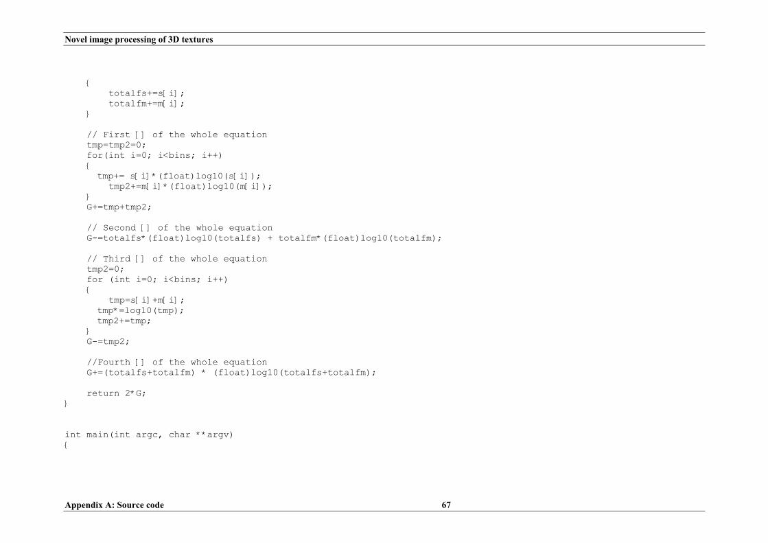
Novel image processing of 3D textures
Appendix A: Source code 67
{ totalfs+=s[i]; totalfm+=m[i]; } // First [] of the whole equation tmp=tmp2=0; for(int i=0; i<bins; i++) { tmp+= s[i]*(float)log10(s[i]); tmp2+=m[i]*(float)log10(m[i]); } G+=tmp+tmp2; // Second [] of the whole equation G-=totalfs*(float)log10(totalfs) + totalfm*(float)log10(totalfm); // Third [] of the whole equation tmp2=0; for (int i=0; i<bins; i++) { tmp=s[i]+m[i]; tmp*=log10(tmp); tmp2+=tmp; } G-=tmp2; //Fourth [] of the whole equation G+=(totalfs+totalfm) * (float)log10(totalfs+totalfm); return 2*G; } int main(int argc, char **argv) {

Novel image processing of 3D textures
Appendix A: Source code 68
char *filename=NULL, *filename2=NULL; char *output = NULL, *output2 = NULL; char *outputfrec = NULL; bool bDoubleImage = false; // printf ("Number of parameters detected: %d\n", argc); if (argc == 1 || argc == 2 && !strcmp(argv[1],"--help")) { printSyntax(); return 0; } if (argc % 2) // Parameter must be an even number { fprintf(stderr, "\nERROR: Incorrect number of parameters.\n\n"); return 1; } for (int i=1; i<argc; i+=2) { if (i==1) filename = argv[1]; else if( !strcmp(argv[i-1],"-o" ) ) output = argv[i]; else if( !strcmp(argv[i-1],"-i") ) { filename2 = argv[i]; bDoubleImage = true; } else if( !strcmp(argv[i-1],"-o2") ) output2 = argv[i]; else if ( !strcmp(argv[i-1],"-f") )

Novel image processing of 3D textures
Appendix A: Source code 69
outputfrec = argv[i]; else { fprintf(stderr, "\nERROR: Unexpectd error in assignment of parameters.\n\n"); return 1; } } if (output2!=NULL && filename2 == NULL) { fprintf(stderr, "\nERROR: -o2 parameter requires -i parameter to be specified beforehand...\n\n"); return 1; } /* printf("Filename is %s, Output is %s\n", filename, output); printf("Filename2 is %s, Output2 is %s and Outputfrec is %s\n", filename2, output2, outputfrec); exit(0); */ // Get image struct image_data im1, *im1_p = &im1, im2, *im2_p = &im2; getimagef(filename, im1_p); float *matrix = im1_p->image32, *matrix2; //Get second image if applicable if (bDoubleImage) { getimagef(filename2, im2_p); matrix2 = im2_p->image32; } // Apply algorith unsigned char *result, *result2; if (matrix == NULL || (bDoubleImage==true && matrix2 == NULL)) {

Novel image processing of 3D textures
Appendix A: Source code 70
fprintf(stderr, "\nERROR: No enough memory available or image file not located...\n\n"); return 1; } /* // Assign random values for (int i=0; i < SIZE; i++) for (int j=0; j < SIZE; j++) matrix[i*SIZE + j]=1 + 256.0*rand() / (RAND_MAX+1.0); */ int *patternstat = new int[36*8]; //36 possible patterns by 8 possible shifts for each one memset(patternstat, 0, sizeof(int));// Reset matrix int height=im1_p->hd.nline, width=im1_p->hd.npix; printf("Calculation in process (%s %dx%d)... \n", filename, height, width); result = (unsigned char *) LBPROT(matrix, height , width, patternstat); // For 2nd image int height2=0, width2=0; if (bDoubleImage) { height2 = im2_p->hd.nline; width2 = im2_p->hd.npix; printf("Calculation in process (%s %dx%d)... \n", filename2, height2, width2); result2 = (unsigned char *) LBPROT(matrix2, height2 , width2); } // Check results if (result == NULL || (bDoubleImage==true && result2 == NULL)) { fprintf(stderr,"ERROR: Calculation aborted...\n"); return 1; } else // Show result { // Store it onto the output file 1 FILE *stream = (output != NULL) ? fopen(output, "w+") : stdout;

Novel image processing of 3D textures
Appendix A: Source code 71
if (stream == NULL) { printf("ERROR: The output file could not be open in writting mode...\n"); return 1; } /*for (int i=1; i<height-1; i++) { for (int j=1; j<width-1; j++) { fprintf(stream, "%d ", result[i*width + j]); } fprintf(stream, "\n"); } */ // Temporal loop: print some internal data for (int i=1; i<2; i++) { for (int j=1; j<width-1; j++) { fprintf(stream, "%2d ", result[i*width + j]); } fprintf(stream, "\n"); } printf("For i=1 and j=2 result is %d\n", result[1*width + 2]); if (output != NULL && (fflush(stream) || fclose(stream))) { fprintf(stderr,"ERROR: Data may not be stored or printed properly...\n"); } // Print pattern statistics int sum, totalpixels= height*width - (2*height + 2*(width-2));//Without edges float perc; fprintf(stream,"\n PATTERN STATISTICS:"); fprintf(stream,"\n -------------------\n"); for (int i=0; i<36; i++)

Novel image processing of 3D textures
Appendix A: Source code 72
{ sum=0; fprintf(stream,"\nPattern %2d --> ", i); for (int j=0;j<8;j++) { fprintf(stream," %6d ", patternstat[8*i + j]); sum+=patternstat[8*i + j]; } perc = (float)(((float)sum/(float)totalpixels)*(float)100.0); fprintf(stream," total = %7d (%2.3f\%)", sum, perc); } fprintf(stream,"\n"); // Store it onto the output file 2 if (output2 != NULL) { FILE *stream2 = (output2 != NULL) ? fopen(output2, "w+") : stdout; if (stream2 == NULL) { printf("ERROR: The second output file could not be open in writting mode...\n"); return 1; } /*for (int i=1; i<height-1; i++) { for (int j=1; j<width-1; j++) { fprintf(stream2, "%d ", result2[i*width + j]); } fprintf(stream2, "\n"); } */ for (int i=1; i<2; i++) { for (int j=1; j<width-1; j++)

Novel image processing of 3D textures
Appendix A: Source code 73
{ fprintf(stream2, "%2d ", result2[i*width + j]); } fprintf(stream2, "\n"); } printf("For i=1 and j=2 result is %d\n", result2[1*width + 2]); if (output2 != NULL && (fflush(stream2) || fclose(stream2))) { fprintf(stderr,"ERROR: Data may not be stored or printed properly...\n"); } } // For image 1 unsigned int *hist = getHistogram(result, height, width, true); // skipEdges=true float *frec = getFrecuencies(hist); /* for (int i=0; i<BINS; i++) printf("Value for bin %d is %d\n", i, hist[i]); */ FILE *stream3 = (outputfrec != NULL) ? fopen(outputfrec, "w+") : stdout; for (int i=0; i<BINS; i++) fprintf(stream3, "%f\n", frec[i]); //fprintf(stream3, "Frecuency for bin %d is %f\n", i, frec[i]); /* float total=0; for (int i=0; i<BINS; i++) total+=frec[i]; printf("Sum of frecuencies is: %f\n\n", total); */ // For image2 if (bDoubleImage) { unsigned int *hist2 = getHistogram(result2, height2, width2, true); // skipEdges=true float *frec2 = getFrecuencies(hist2);

Novel image processing of 3D textures
Appendix A: Source code 74
fprintf(stream3, "\n"); for (int i=0; i<BINS; i++) fprintf(stream3, "%f\n", frec2[i]); //printf("Frecuency for bin %d is %f\n", i, frec2[i]); /* float total2=0; for (int i=0; i<BINS; i++) total2+=frec[i]; printf("Sum of frecuencies is: %f\n", total2); */ printf("\nG statistic: %f\n", getGStatistic(frec, frec2)); delete [] hist2; // Free memory delete [] frec2; // Free memory delete [] result2; // Free memory delete [] matrix2; // Free image memory = im2_p->image32 matrix } delete [] hist; // Free memory delete [] frec; // Free memory delete [] result; // Free memory } // Free memory delete [] matrix; // Free image memory = im1_p->image32 matrix printf("LBPROT fisnihed successfully!\n"); return 0; }

Novel image processing of 3D textures
Appendix B: Excel format files 75
Appendix B: Excel format files
• Directionality research files: o Unidirectional
aaa-Pattern-Stat.xls adj-Pattern-Stat.xls
o Bidirectional ach-Pattern-Stat.xls afe-Pattern-Stat.xls
o Multidirectional aar-Pattern-Stat.xls acc-Pattern-Stat.xls
• Variability reach files: Pattern-Stat-Parts-45.90.xls Comparison between 1.acc.0.45.90.part1 and 1.acc.0.60.90.part1.xls Comparison of 0.aaa.0.45.x images.xls Comparison of 0.aaa.0.60.x images.xls Comparison of 0.aaa.0.75.x images.xls Distribution part1-4 of 1.acc.0.45.90.xls
• G statistic research files: G-Statistic 0.x.0.45.90 images comparison.xls G-Stat-Parts-45.90.xls