Department of Engineering Physics and Mathematics

Laboratory of Biomedical Engineering

Helsinki University of Technology

Espoo, Finland

Cardiomagnetic Source Imaging

Katja Pesola

Dissertation for the degree of Doctor of Science in Technology to bepresented with due permission for public examination and debate in Au-ditorium F1 at Helsinki University of Technology (Espoo, Finland) onthe 19th of May, 2000, at 12 o’clock noon.

Espoo 2000

ISBN 951–22–4962–6Printing house Picaset, Helsinki 2000

i

Contents

List of publications iii

Summary of publications iv

List of abbreviations viii

List of symbols ix

1 Introduction 1

2 Modeling of volume conductor and current source 4

2.1 Biolectric current sources and the activation of the heart . . . . . . . . . . . 4

2.2 Quasistatic approximation . . . . . . . . . . . . . . . . . . . . . . . . . . . . 6

2.3 Piecewise homogeneous volume conductor . . . . . . . . . . . . . . . . . . . 7

2.4 Boundary element approximation . . . . . . . . . . . . . . . . . . . . . . . . 8

2.4.1 Constant potential approach . . . . . . . . . . . . . . . . . . . . . . . 8

2.4.2 Linearly varying surface potentials . . . . . . . . . . . . . . . . . . . 10

2.4.3 Higher–order elements . . . . . . . . . . . . . . . . . . . . . . . . . . 11

2.5 Modeling of the current source . . . . . . . . . . . . . . . . . . . . . . . . . . 11

2.5.1 Point–like source models . . . . . . . . . . . . . . . . . . . . . . . . . 12

2.5.2 Distributed source models . . . . . . . . . . . . . . . . . . . . . . . . 12

3 Current dipole localization 14

3.1 Calculation methods . . . . . . . . . . . . . . . . . . . . . . . . . . . . . . . 14

3.2 Simulation studies . . . . . . . . . . . . . . . . . . . . . . . . . . . . . . . . 15

3.3 Phantom and animal studies . . . . . . . . . . . . . . . . . . . . . . . . . . . 15

3.4 Patient measurements . . . . . . . . . . . . . . . . . . . . . . . . . . . . . . 18

3.5 Effect of torso modeling . . . . . . . . . . . . . . . . . . . . . . . . . . . . . 20

4 Equivalent current density 24

4.1 Lead fields . . . . . . . . . . . . . . . . . . . . . . . . . . . . . . . . . . . . . 24

4.2 Regularization . . . . . . . . . . . . . . . . . . . . . . . . . . . . . . . . . . . 25

4.2.1 Truncated SVD . . . . . . . . . . . . . . . . . . . . . . . . . . . . . . 26

4.2.2 Tikhonov regularization . . . . . . . . . . . . . . . . . . . . . . . . . 26

4.3 Weighted solutions . . . . . . . . . . . . . . . . . . . . . . . . . . . . . . . . 30

4.4 Temporal and statistical regularization . . . . . . . . . . . . . . . . . . . . . 31

4.5 Applications of CDE . . . . . . . . . . . . . . . . . . . . . . . . . . . . . . . 32

4.5.1 Ischemia studies . . . . . . . . . . . . . . . . . . . . . . . . . . . . . . 32

4.5.2 Other clinical studies . . . . . . . . . . . . . . . . . . . . . . . . . . . 35

ii

5 Uniform double layer 36

5.1 Formulation of the UDL model . . . . . . . . . . . . . . . . . . . . . . . . . 36

5.2 Clinical studies . . . . . . . . . . . . . . . . . . . . . . . . . . . . . . . . . . 39

6 Cardiomagnetic instrumentation 42

6.1 BioMag Laboratory . . . . . . . . . . . . . . . . . . . . . . . . . . . . . . . . 42

6.2 Other research sites . . . . . . . . . . . . . . . . . . . . . . . . . . . . . . . . 44

6.3 Requirements and future development . . . . . . . . . . . . . . . . . . . . . . 45

7 Discussion 47

7.1 The role of anisotropy . . . . . . . . . . . . . . . . . . . . . . . . . . . . . . 47

7.2 MCG vs. ECG . . . . . . . . . . . . . . . . . . . . . . . . . . . . . . . . . . 48

7.2.1 Theoretical considerations . . . . . . . . . . . . . . . . . . . . . . . . 48

7.2.2 Experimental observations . . . . . . . . . . . . . . . . . . . . . . . . 49

7.3 Other functional imaging techniques . . . . . . . . . . . . . . . . . . . . . . 50

7.4 Future aspects . . . . . . . . . . . . . . . . . . . . . . . . . . . . . . . . . . . 50

Acknowledgments 52

References 53

iii

List of publications

This thesis consists of an overview and of the following eight publications:

I K. Pesola, U. Tenner, J. Nenonen, P. Endt, H. Brauer, U. Leder, and T. Katila:

Multichannel magnetocardiographic measurements with a physical thorax phantom.

Medical & Biological Engineering & Computing 37, pp. 2–7, 1999.

II R. Fenici, J. Nenonen, K. Pesola, P. Korhonen, J. Lotjonen, M. Makijarvi, L. Toivonen,

V–P. Poutanen, P. Keto, and T. Katila: Nonfluoroscopic localisation of an amagnetic

stimulation catheter by multichannel magnetocardiography. Pacing and Clinical Elec-

trophysiology 22, pp. 1210–1220, 1999.

III K. Pesola, J. Nenonen, R. Fenici, J. Lotjonen, M. Makijarvi, P. Fenici, P. Korhonen,

K. Lauerma, M. Valkonen, L. Toivonen, and T. Katila: Bioelectromagnetic localization

of a pacing catheter in the heart. Physics in Medicine and Biology 44, pp. 2565–2578,

1999.

IV K. Pesola, J. Lotjonen, J. Nenonen, I.E. Magnin, K. Lauerma, R. Fenici, and T. Katila:

The effect of geometric and topologic differences in boundary element models on mag-

netocardiographic localization accuracy. Accepted for publication in IEEE Transac-

tions on Biomedical Engineering, 2000.

V K. Pesola, J. Nenonen, R. Fenici, and T. Katila: Comparison of regularization methods

when applied to epicardial minimum norm estimates. Biomedizinische Technik 42

(Suppl. 1), pp. 273–276, 1997.

VI K. Pesola, H. Hanninen, K. Lauerma, J. Lotjonen, M. Makijarvi, J. Nenonen, P. Takala,

L.–M. Voipio–Pulkki, L. Toivonen, and T. Katila: Current density estimation on the

left ventricular epicardium: A potential method for ischemia localization. Biomedi-

zinische Technik 44 (Suppl. 2), pp. 143–146, 1999.

VII T. Oostendorp and K. Pesola: Non–invasive determination of the activation sequence

of the heart: Validation by comparison with invasive human data. In A. Murray and

S. Swiryn (Eds.): Computers in Cardiology 25, pp. 313–316, 1998.

VIII K. Pesola, T. Oostendorp, J. Nenonen, P. Korhonen, J. Lotjonen, L. Toivonen, and

T. Katila: Uniform double layer solutions for magnetocardiographic and body sur-

face potential mapping data. In T. Yoshimoto, M. Kotani, S. Kuriki, H. Karibe and

N. Nakasato (Eds.): Recent Advances in Biomagnetism: Proceedings of the 11th Inter-

national Conference on Biomagnetism, Tohoku University Press, Sendai, pp. 290–293,

1999.

iv

Summary of publications

The eight publications included in this thesis are the result of team work carried out at the

Laboratory of Biomedical Engineering between the technical experts, medical collaborators

from the Helsinki University Central Hospital and foreign researchers in the field of electro–

and magnetocardiography. The author has actively taken part in the research work presented

in the publications. In the following, a brief summary of each publication and the statement

of the author’s involvement will be provided.

I: Multichannel magnetocardiographic measurements with a physical thorax

phantom (Medical & Biological Engineering & Computing 37, pp. 2–7, 1999)

In this work, a novel non–magnetic thorax phantom and artificial dipolar sources were

applied in assessing the accuracy of magnetocardiographic (MCG) equivalent current

dipole (ECD) localizations. The data were recorded in the same clinical environment

where the patient studies are carried out. The localizations were found to be accurate

within a few millimeters, provided that the signal–to–noise ratio (SNR) and the good-

ness of fit of the localizations were sufficiently high. The dependence of the goodness of

fit on the SNR was derived, and the experimental results were found to correspond to

the derived model. The ECD localization accuracies obtained in this study, evaluated

in certain ranges of the SNR and of the goodness of fit, are an indication of the best

possible accuracy achievable in clinical studies.

II: Nonfluoroscopic localization of an amagnetic stimulation catheter by

multichannel magnetocardiography (Pacing and Clinical Electrophysiology 22,

pp. 1210–1220, 1999)

The accuracy of magnetocardiographic ECD localizations was investigated in five pa-

tients using a non–magnetic stimulation catheter. The position of the tip of the

catheter was documented on biplane cine X–ray images. MCG signals were then

recorded during cardiac pacing. Non–invasive localizations of the tip of the catheter

were computed using individual, homogeneous boundary element models to model the

torso. The mean distance between the tip of the catheter determined from fluoroscopy

and MCG localizations was 11 ± 4 mm. The mean distance between the localizations

calculated during the stimulus spikes and in the beginning of the evoked responses was

4 ± 1 mm. The accurate 3D localizations of the tip of the catheter suggest that the

MCG method could be developed towards a useful clinical tool during electrophysio-

logical studies.

v

III: Bioelectromagnetic localization of a pacing catheter in the heart (Physics in

Medicine and Biology 44, pp. 2565–2578, 1999)

In this work, the non–magnetic catheter was applied in 10 patients. Biplane fluoro-

scopic imaging with lead ball markers was again used to record the catheter position.

In addition to the MCG recordings, simultaneous multichannel body surface poten-

tial mapping (BSPM) recordings were performed at the BioMag Laboratory during

catheter pacing. ECD localizations were computed from MCG and BSPM data, em-

ploying standard and patient–specific boundary element torso models. Using individual

models with the lungs included, the average MCG localization error was 7 ± 3 mm,

whereas the average BSPM localization error was 25 ± 4 mm. The results of this study

indicate that the accuracy of ECD localizations calculated from MCG data is superior

to the accuracy obtainable from BSPM measurements.

IV: The effect of geometric and topologic differences in boundary element mod-

els on magnetocardiographic localization accuracy (Accepted for publication in

IEEE Transactions on Biomedical Engineering, 2000)

The study was performed to evaluate the changes in MCG dipole localization results

when the geometry and the topology of the torso model were altered. Three reference

torso models were manipulated to mimic various sources of error in the measurement

and analysis procedures. The effect of each modification was investigated by calculating

3D distances from the “gold standard” ECD localizations, obtained with the reference

models, to the locations obtained with the modified models. The effect of inhomo-

geneities (lungs, intra–ventricular blood) was found to be significant for deep source

locations. However, superficial sources could be localized within a few millimeters even

with non–individual torso models. In general, the thorax model should extend long

enough in the pelvic region, and the positions of the lungs and the ventricles should

be known in order to obtain accurate localizations.

V: Comparison of regularization methods when applied to epicardial minimum

norm estimates (Biomedizinische Technik 42 (Suppl. 1), pp. 273–276, 1997)

In this study, MCG measurements of five patients with the non–magnetic catheter

in the heart were used to validate the calculated minimum norm, or current density,

estimates. The estimates were computed at the stimulus spikes and during the follow-

ing depolarization on the triangulated epicardial surfaces using different regularization

techniques. The applied techniques were: (i) the truncation of the singular value de-

composition, (ii) Tikhonov regularization, (iii) weighting and (iv) recursive weighting.

When the Tikhonov method was used, the value of the regularization parameter was

determined by means of the L–curve. In techniques (iii) and (iv), the square roots of

vi

the optimal dipole amplitudes were applied. The results of the study showed that when

the source was located within 8 cm from the sensors, all regularization techniques were

able to localize the center point of the source current distribution correctly. However,

the estimates calculated for a relatively deep source (13 cm away from the sensors)

clearly showed the need for weighting. In this case, the techniques (i) and (ii) failed to

give a meaningful description about the underlying activity.

VI: Current density estimation on the left ventricular epicardium: A potential

method for ischemia localization (Biomedizinische Technik 44 (Suppl. 2), pp. 143–

146, 1999)

Different regularization operators applicable in Tikhonov regularization were tested

by calculating current density estimates (CDEs) from simulated MCG data on the

epicardial surface of the left ventricle. Second–order regularization was found to be

superior to zero–order regularization. In addition to simulations, CDE was applied in

13 coronary artery disease (CAD) patients. MCG measurements were performed at

rest and after stress using a non–magnetic exercise ergometer. CDEs were calculated

from the ST–segment difference signals. In four single–vessel CAD patients, an increase

in the CDE amplitude was found to correlate with the expected ischemic myocardial

region. In nine three–vessel CAD patients, PET was used as a reference in separating

the areas of viable myocardial tissue from scar regions. In this patient group, the areas

of low CDE amplitude were found to match with scar regions whereas a high CDE

amplitude was found to correlate with viable areas.

VII: Non–invasive determination of the activation sequence of the heart: Valida-

tion by comparison with invasive human data (In: A. Murray, S. Swiryn (Eds.):

Computers in Cardiology 25, pp. 313–316, 1998)

In this paper, results from a validation study carried out with the uniform double

layer (UDL) source model were presented. Invasive human data obtained from four

patients with an old myocardial infarction that underwent open–chest surgery in order

to treat ventricular arrhythmia were used in the validation. During surgery, the epi-

cardial activation was mapped by using an electrode sock wrapped around the heart.

The invasively determined activation maps were compared to the calculated activa-

tion times, obtained from BSPM data measured prior to surgery. The overall patterns

(such as breakthroughs and regions of late activation) were reproduced quite well in

the computed data sets. However, there was a clear difference in the precise locations

of these sites. This could be caused by the uncertainty in the positions of the epicar-

dial electrodes, or by the infarcted regions for which the assumption about a uniform

double layer does not hold.

vii

VIII: Uniform double layer solutions for magnetocardiographic and body surface

potential mapping data (In: T. Yoshimoto, M. Kotani, S. Kuriki, H. Karibe and

N. Nakasato (Eds.): Recent Advances in Biomagnetism: Proceedings of the 11th Inter-

national Conference on Biomagnetism, Tohoku University Press, Sendai, pp. 290–293,

1999)

In this study, the properties and the accuracy of the ventricular activation times, calcu-

lated from MCG data, were compared to those of invasive and BSPM data presented in

Publication VII. The qualitative comparison between the measured and the calculated

epicardial activation times showed that the calculated maps were, in general, in good

agreement with the measured data. However, certain differences were present both in

the MCG and BSPM maps. In the quantitative comparison, the activation times at

the electrode locations, calculated from MCG data, had an average relative difference

of 29 % with respect to the measured data while for BSPM maps the average relative

difference was found to be 37 %. However, more accurate information about the lo-

cations of the invasive electrodes would be necessary to make a reliable quantitative

comparison.

Statement of involvement

In Publication I, the author performed the magnetic measurements with the physical

thorax phantom together with Dr. Uwe Tenner and carried out the analysis of the measure-

ments. Publication I was also written by the author. Publications II and III are the result

of a co–operation with Prof. Riccardo Fenici from the Catholic University of Rome, Italy. In

Publication II, the author was mainly responsible for performing the MCG recordings at the

BioMag Laboratory as well as participated actively in computing the ECD localizations and

analyzing the X–ray results. In Publication III, the author was responsible for carrying out

the simultaneous MCG and BSPM recordings and a large share of the analysis of the data.

Publication III was also written by the author. In Publication IV, the ECD calculations

were performed by the author, and it was written in co–operation with Dr. Jyrki Lotjonen.

The calculation of the current density estimates in Publications V and VI was implemented

and performed by the author. The publications were also written by her. Publications VII

and VIII are the result of a collaboration with Dr. Thom Oostendorp from the University of

Nijmegen, the Netherlands. The author has performed most of the inverse calculations from

MCG and BSPM data, as well as written Publication VIII.

viii

List of abbreviations

The most important abbreviations used in the overview are listed and explained below.

AT activation timeAV atrio–ventricularBE boundary elementBEM boundary element methodBSPM body surface potential mappingCAD coronary artery diseaseCDE current density estimateCEF cardiac evoked fieldCEP cardiac evoked potentialDC direct currentECD equivalent current dipoleECG electrocardiographyEP electrophysiologicalFEM finite element methodgSVD generalized singular value decompositionHTC high–temperatureHUCH Helsinki University Central HospitalHUT Helsinki University of TechnologyLAD left anterior descending coronary arteryLCX left circumflex coronary arteryLTC low–temperatureLV left ventricleLVH left ventricular hypertrophyMCG magnetocardiographyMI myocardial infarctionMNE minimum norm estimateMR magnetic resonanceMRI magnetic resonance imagingPET positron emission tomographyRCA right coronary arteryRF radio–frequencyRMS root–mean–squareRV right ventricleSA sino–atrialSNR signal–to–noise ratioSQUID superconducting quantum interference deviceSVD singular value decompositiontSVD truncated singular value decompositionUDL uniform double layerVT ventricular tachycardiaWPW Wolff–Parkinson–White

ix

List of symbols

The most important symbols of the overview are listed and shortly explained below. Vectorsand vector functions are denoted with boldface letters.

Ji (microscopic) impressed current density [A/m2]Jp (macroscopic) primary current density [A/m2]Jv volume current density [A/m2]Jtot total (quasi–static) current density [A/m2]E electric field [V/m]B magnetic flux density [T] (in this thesis referred to as the magnetic field)∇ gradient operator (nabla)ρ total charge density [C/m3]ε0 electric permittivity in vacuum [F/m]µ0 magnetic permeability in vacuum [H/m]σ electric conductivity [S/m]φ electric potential [V]r position vector referring to an observation (field) pointr ′ position vector referring to an integration (source) pointV ′ a bounded volume conductor containing the current sourcesSk bounding surface in a piecewise homogeneous torso modelM number of surfaces in a piecewise homogeneous torso modelhi(·) basis function in boundary element formulation∆i flat triangular boundary elementΩ solid angle matrixI identity matrixg goodness of fitm number of sensorsn number of source pointsLi magnetic lead field vector of the ith sensorL lead field matrixΓ inner product matrix of the lead fieldsJ∗ minimum norm estimateJ current density estimateλ regularization parameterR regularization operatorD2 discrete approximation of the surface Laplacianµi generalized singular valueκ curvature functionD weighting (or pre–conditioning) matrixF magnetic field component or electric potential in the UDL formulationA(·, ·) magnetic or electric transfer function in the UDL formulationH(·) Heaviside step functionτ activation time on the ventricular surface [s]

1

1 Introduction

The electric current related to the functioning of the human heart causes differences in the

electric potential inside the body. The measurement of these potential differences on the

body surface, known as electrocardiography (ECG), was developed as a clinical tool already

in the beginning of the 20th century. By now, the ECG has established an important role in

clinical diagnosis and research of the cardiac function (e.g., MacFarlane and Lawrie 1988).

In a more recent approach, ECG signals are collected with an electrode array to achieve

denser spatial sampling. Measuring ECGs this way is usually referred to as body surface

potential mapping (BSPM) since the anterior and posterior surfaces of the upper body (the

torso) are covered with electrodes.

The same current sources in the heart generating the ECG also give rise to a magnetic

field inside and outside of the body. The magnetic field produced by the heart was first

measured by Baule and McFee (1963). This result gave birth to magnetocardiography (MCG)

(e.g., Siltanen 1988). The maximum amplitude of the magnetic field generated by the human

heart, approximately 10−10 T, is several orders of amplitude weaker than the earth’s magnetic

field. Therefore, the detection of MCG requires sensitive detectors and usually also shielding

against external magnetic disturbances. Nowadays, the detection of MCG is based on highly

sensitive sensors, Superconducting QUantum Interference Devices (SQUIDs), which were

invented in the 1960’s. In an MCG measurement, the sensors are usually arranged in a plane

or in a concave surface close to the chest of the patient. The measurement is completely

non–invasive, i.e. no contact, external media, electromagnetic fields or other radiation are

directed towards the subject to be measured. As with ECG signals, information about the

function of the heart is obtained with millisecond time resolution.

Estimating the bioelectric current sources in the body from biomagnetic measurements is

often referred to as magnetic source imaging or functional source localization (e.g., Hamalai-

nen and Nenonen 1999). Therefore, the corresponding estimation in the heart is called

cardiomagnetic source imaging. With a high enough localization accuracy of the current

sources in the heart, valuable information can be provided, e.g., for the pre–ablative eval-

uation of arrhythmia patients. This evaluation is of special importance since nowadays

the radio–frequency (RF) catheter ablation has replaced antiarrhythmic drug therapy for

the treatment of many types of cardiac arrhythmias (Morady 1999). For example, in the

Wolff–Parkinson–White (WPW) patient group with an accessory conducting pathway from

the atria into the ventricles, RF ablation has eliminated the need for surgical ablation in

almost all patients and the need for antiarrhythmic–drug therapy in many patients. The

efficacy of catheter ablation depends on the accurate identification of the site of the ori-

gin of arrhythmia. Successful MCG results have been reported in locating the abnormal

ventricular pre–excitation sites associated with the WPW–syndrome, origin of ventricular

2 1 INTRODUCTION

extrasystolic beats, and origin of atrial arrhytmias (e.g., Nenonen et al 1991a, Ribeiro et al

1992, Weismuller et al 1992, Fenici and Melillo 1993, Makijarvi et al 1993, Oeff and Burghoff

1994, Moshage et al 1996). A prolonged exposure to radiation can therefore be reduced by

taking into account the MCG localization result in the ablation procedure. Furthermore,

preliminary studies also carried out in this thesis indicate that ischemic areas, i.e. areas which

are suffering from lack of oxygen, and infarcted regions could be localized from multichannel

MCG recordings. In addition to localization studies, multichannel MCG and BSPM studies

have shown to be especially promising in evaluating the risk of life–threatening arrhythmias

in different cardiac pathologies, especially after myocardial infarction (e.g., Montonen et al

1995, Hubley–Kozey et al 1995). A recent review on MCG and BSPM studies has been

presented by Stroink et al (1996), and on magnetic source imaging in the brain and in the

heart by Hamalainen and Nenonen (1999).

In source localization studies, the forward problem has to be solved first, i.e. one has to

calculate the electric potential or the magnetic field, generated by the current sources in the

heart, on and outside of the body, respectively. In the inverse problem, the current source

is determined from the MCG and/or BSPM measurements. However, even with a complete

knowledge of the electromagnetic field outside of the source region, the inverse problem

cannot be uniquely solved because the same field distribution can be produced by infinitely

many current source configurations. Therefore, restrictive assumptions about the current

sources are needed. The conventional way is to use equivalent source models for describing

the actual currents. The parameters of the source model can then be determined from the

measured data, e.g., in a least–squares sense. In addition to the current source, the media

surrounding it needs to modeled. The volume conductor models used in cardiomagnetic

source imaging studies are usually referred to as torso models.

In this thesis, the aim was to investigate the obtaible accuracy of cardiomagnetic source

imaging results using different source models. In addition, the effect of the torso model

on the localization accuracy was examined. In some studies, also body surface potential

mapping data were used for comparison purposes. A high impact was given to clinical ap-

plications, i.e. how the calculation methods would work in patients. In Section 2, the basic

theory related to modeling the torso and the current sources inside the heart is presented

as background information. The most commonly used source model, the equivalent current

dipole (ECD), and studies related to it are described in Section 3. The obtainable accuracy

of ECD localizations was investigated inside a phantom by using artificial current sources

and in patients by using a non–magnetic stimulation catheter. In addition, the effect of

torso modeling on MCG dipole localization accuracy was thoroughly evaluated. In Sec-

tion 4, calculation methods suitable for solving an equivalent current density are presented.

These methods were developed and applied with simulated and measured MCG data. The

uniform double layer (UDL) source model, which can be used in representing the spread

3

of the ventricular activation, was also studied by using invasively measured epicardial po-

tential data for validation. The UDL model is described in Section 5. The main research

centers currently involved in cardiomagnetic studies, especially the BioMag Laboratory at

the Helsinki University Central Hospital (HUCH) where all the magnetic measurements ana-

lyzed in this thesis were performed, are presented in Section 6. Section 7 contains discussion

about cardiomagnetic source imaging as well as it’s future aspects.

4 2 MODELING OF VOLUME CONDUCTOR AND CURRENT SOURCE

2 Modeling of volume conductor and current source

In the following, the genesis of the bioelectric current sources inside the heart is briefly

described. Thereafter, the well–known integral equations suitable for treating the problem

in terms of bounding surfaces inside an inhomogeneous volume conductor (Barnard et al

1967a, 1967b, Geselowitz 1967, 1970, Horacek 1973) are presented. The formulation based on

the bounding surfaces is needed in the calculations based on the boundary element method

in which the surfaces are tessellated with geometrical elements. Finally, the concepts of

the forward and the inverse problems are introduced. Since the inverse problem has no

unique solution, the current source inside the heart is usually described with a source model,

characterized by the values of the model parameters. The most commonly–used source

models, applied in solving the cardiac inverse problem, will also be described. The source

models investigated in this thesis and the estimation methods used in solving the values of

the model parameters will be presented in the following sections.

2.1 Biolectric current sources and the activation of the heart

A cardiac cell at rest exposes a potential difference between the intra– and extracellular

spaces so that the interior of the cell has a negative potential relative to the exterior. This

potential difference is caused by the differences in the permeability of the cell membrane to

different ions and by the ion pumps in the membrane. In the resting state, the cell membrane

is rather permeable to potassium (K+) ions whereas the permeability for the sodium (Na+)

ions is low. Therefore, the resting potential has a negative value close to the Nernst potential

of K+ ions, approximately between −80 mV and –95 mV. As a response to a stimulus, the

permeability of the cell membrane to Na+ ions increases. Thus, Na+ starts to flow across

the membrane causing the potential difference over the membrane to approach the Nernst

potential of Na+ which has a positive value. The amplitude of the change in the membrane

voltage of a normal cardiac muscle cell is about 100 mV. The electrical activation results

in the mechanical contraction of a muscle cell which is initiated by the influx of calcium

(Ca2+) ions, which further release Ca2+ ions inside the cell. The fast depolarization phase is

followed by a plateau phase in the membrane potential, lasting approximately 200–300 ms.

After the plateau phase, the membrane potential returns to it’s original value. During the

process, the cell is refractory, i.e. unable to respond to an additional electrical stimulus.

The activation cycle of a healthy heart is initiated by the sino–atrial (SA) node, located

above the right atrium. In the special pacemaker cells of the SA node, the value of the

membrane potential increases until the threshold for the opening of the Na+ ion channels is

reached. From the SA node, the electrical activation spreads along the internodal tracts in

the atria thus depolarizing the atrial muscle cells. A phase of slow conduction is occurring

in the atrio–ventricular (AV) node in the border of the atria and the ventricles. In the

5

Fig. 1: The time courses of the membrane potentials during the electrical excitation of theheart: the SA node, the atria, the AV node, the bundle of His, the bundle branches, thePurkinje fibers and the ventricular muscle (Netter 1991).

ventricles, the activation spreads along the bundle of His, the right and left bundle branches

and the Purkinje fibers which efficiently initiate the depolarization of the endocardial muscle

cells. The excitation finally spreads from the endocardium towards the epicardium. The

whole ventricular muscle is normally activated within 100 ms. The shapes of the membrane

potentials in different types of cardiac cells is presented in Fig. 1, along with their timing with

respect to an ECG signal measurable on the body surface. The form of the corresponding

MCG signal closely resembles to the shape of the ECG signal. The activation of the atria

causes the P–wave whereas the excitation of the ventricles causes the QRS–complex to appear

in the ECG signal. The repolarization of the atria is hidden underneath the QRS–complex

while the repolarization of the ventricles results in the T–wave.

The electric current flowing through the cell membrane is usually referred to as the

microscopic impressed current density Ji (Plonsey 1969). The resulting magnetic field or the

changes in the electric potential due to the impressed current flowing in one cardiac cell are

too minor to be measured outside of the body. However, the activation in the heart spreads as

a wavefront, and therefore several cells are activated simultaneously. When the macroscopic

current distribution related to the activation of the heart is considered, it is customary to

speak about the primary current density Jp. The primary current density is restricted to

the electrically active tissue (Tripp 1983), and it can be defined as the difference between

the total current density Jtot and the passive, ohmic volume current Jv: Jp = Jtot − Jv.

The volume current Jv is the result of the macroscopic electric field on charge carriers in the

conducting medium (Hamalainen and Nenonen 1999). The primary current is the target of

6 2 MODELING OF VOLUME CONDUCTOR AND CURRENT SOURCE

interest in solving the inverse problem. Because the volume current also contributes to the

electric (E) and magnetic (B) fields, it has to be taken into account in the solutions.

2.2 Quasistatic approximation

As the total current density Jtot in the body is time–dependent, the generated electric

and magnetic fields also vary with time. In the human body, the capacitive component

of tissue impedance has been found to be negligible in the frequency band (< 1000 Hz)

of internal bioelectric events (Plonsey 1969). Therefore, the time–varying electric potential

and magnetic field in the human body can be assumed in most cases to behave as if they

were quasi–stationary. According to this approximation, the true time–dependent field terms

(∂E/∂t, ∂B/∂t) in Maxwell’s equations can be left out, and the quasi–static equations can

be expressed as

∇ · E = ρ/ε , ∇× E = 0 ,

∇ ·B = 0 , ∇×B = µ0(Jtot +∇×M) ,

where ρ is the total charge density and ε = εrε0, where εr is the relative electric permittivity

of the medium and ε0 is the electric permittivity of vacuum. The magnetic permeability

of vacuum is denoted with µ0 and the magnetization of the medium with M. Usually it is

assumed that M has no effect on the field B.

The total current density Jtot can be divided into two components as explained before.

The ohmic volume current relates directly to the electric field as Jv = σE, where σ is the

electric conductivity of the medium. Because the curl of the electric field vanishes, the

electric field can be written as a gradient of a scalar potential E = −∇φ. Therefore, the

total current density can be expressed as Jtot = Jp − σ∇φ. Because the divergence of the

total current density vanishes, the following Poisson equation is valid for a region containing

primary sources:

∇ · Jp = ∇ · (σ∇φ) . (1)

If no primary sources are present, Eq. 1 turns into the Laplace equation ∇ · (σ∇φ) = 0. In

a general case, the electric conductivity σ may be anisotropic, i.e. the conductivity varies as

a function of direction. In such a case, σ in Eq. 1 can be expressed as a tensor.

The integral form of the curl equation for the magnetic field presents the Ampere–Laplace

law:

B(r) =µ0

4π

∫V ′

Jtot(r′)× (r− r ′)

|r− r ′|3 dv′ , (2)

where r is the observation (field) point, r ′ is the integration (source) point, and the inte-

gration volume V ′ contains all sources. By including the separation of the total current into

primary and volume current components, Eq. 2 can be expressed as (Geselowitz 1970)

B(r) =µ0

4π

∫V ′(Jp(r

′) + φ(r ′)∇′σ(r ′))× (r− r ′)|r− r ′|3 dv′ . (3)

7

Eq. 3 shows that in the case of an infinite homogeneous volume conductor, the second term

in the integral vanishes, and the magnetic field depends only on the primary current. Also

in special kind of bounded volume conductors, such as a sphere and an infinite half–space,

the radial component of the magnetic field, which is usually to be measured, is unaffected

by the conductivity difference over the bounding surface. The sphere model is often applied

in brain studies, and the infinite half–space has been used, e.g., to approximate the anterior

surface of the torso in heart studies.

In the general case, the volume conductor may contain regions with different and even

anisotropic electric conductivities. In such a case, the electric potential and the magnetic

field in the whole volume conductor will have to be solved from Eqs. 1 and 2, e.g., with

the finite element method (FEM) (e.g., Czapski et al 1996 and Klepfer et al 1997) or with

the finite difference method (FDM). In cardiomagnetic source imaging studies, however, the

volume conductor is usually modeled as piecewise homogeneous. In this case, the boundary

element method (BEM) (e.g., Brebbia et al 1984) can be used in the calculations. In BEM, the

computational demands will be smaller than in FEM or FDM. The BEM is used throughout

this thesis.

2.3 Piecewise homogeneous volume conductor

In the following, we assume a piecewise homogeneous volume conductor consisting of M

different regions. Each region has a constant and isotropic conductivity, σk, and is bounded

by the surface Sk. In this case, the gradient of the conductivity vanishes everywhere else

except at the borders of the regions, and the volume integral of the second term in Eq. 3

can be turned into a surface integral (Geselowitz 1970):

B(r) = B∞(r)− µo

4π

M∑k=1

(σ′k − σ′′

k)∫

Sk

φSkdSk × (r− r ′)

|r− r ′|3 , (4)

where σ′k and σ′′

k are the conductivities inside and outside of the surface Sk, respectively.

The primary current density Jp produces the magnetic field B∞ in an infinite homogeneous

volume conductor, and dSk = n dSk is a vector element of surface Sk, oriented along the

outward unit normal n.

The electric potential φSlon the surface Sl in a piecewise homogeneous volume conductor

can be obtained from Eq. 1 by applying the proper boundary conditions and by using the

Green’s theorem (Barnard et al 1967a, 1967b, Geselowitz 1967, Horacek 1973):

φSl(r) =

2σs

(σ′l + σ′′

l )φ∞(r)− 1

2π

M∑k=1

(σ′k − σ′′

k)

(σ′l + σ′′

l )

∫Sk

φSkdSk · (r− r ′)

|r− r ′|3 , (5)

where σs is the electric conductivity at the source location and φ∞ the electric potential in

an infinite homogeneous volume conductor. The conductivity on the surface Sl is defined as

8 2 MODELING OF VOLUME CONDUCTOR AND CURRENT SOURCE

the average of the conductivities inside and outside of the surface: σSl= 1

2(σ

′′l + σ

′l). Since

the unknown potential functions are inside the integrand, Eqs. 4 and 5 are not analytically

solvable in a general case. However, they can be solved numerically with the BEM. The

boundary element (BE) torso models used in the MCG inverse calculations typically contain

at least the surface of the torso. Improvements in the torso models can be obtained by

including the lungs and the intraventricular blood masses. The torso models can be recon-

structed, e.g., from magnetic resonance (MR) images. Recently, automated methods have

been developed for the reconstruction of BE models (Lotjonen 2000). The modeling of the

volume conductor will be further addressed in section 3.5.

2.4 Boundary element approximation

In the boundary element method, an approximate solution φ for the potential on the bound-

ing surfaces can be obtained by representing the surfaces in simplified forms and by approx-

imating the potential with a set of basis functions. The bounding surfaces, separating the

regions with different conductivities, are tessellated with geometrical elements. This reduces

the surface integrals in Eqs. 4 and 5 to summations of surface integrals over the elements.

The approximate solution φ is defined as a linear combination of Nf basis functions, denoted

by h1, · · · , hNf, such that

φ(r) =Nf∑i=1

αihi(r) , (6)

where αi are scalar coefficients and r is a point on one of the bounding surfaces. The sum

of the basis functions in any r is restricted to one.

Flat triangular elements, denoted as ∆i, are most commonly used in the biomagnetic cal-

culations. With these elements, constant or linear potential approximations can be applied

which have also been used in this thesis. Higher–order elements, such as curved triangles (Fri-

jns et al 2000, Gencer and Tanzer 1999) and 8–noded isoparametric quadrilateral elements

(Wach et al 1997, Fischer et al 1998, 1999a), have also been introduced in the literature. A

brief description of the different approximations will be given in the following.

2.4.1 Constant potential approach

In the constant potential approximation, the center points of the triangles are used as the

discretization points. The potential is assumed to be constant over each triangle, resulting

in the most simple set of basis functions:

hi(r) =

1 if r ∈ ∆i

0 otherwise. (7)

Therefore, the integration in Eqs. 4 and 5 can be reduced to summations over the constant

potential values, multiplied by the solid angle factors Ωij = − 12π

∫∆jnjd∆j(r

′) · ci−r ′|ci−r ′|3 ,

9

where Ωij is the solid angle (divided by 2π) subtended by the triangle ∆j at the centroid

ci of triangle ∆i, and nj is the outward unit normal of triangle ∆j. The value of the solid

angle for a plane triangle can be calculated analytically (van Oosterom and Strackee 1983),

and Eq. 5 can be discretized into

φl = gl +M∑

k=1

ωlkφk, l = 1, . . . ,M , (8)

where the vectors φl and gl contain the values φli and gl

i = (2σsφl∞,i)/(σ

′′l + σ

′l) in each

triangular element ∆li of the surface Sl. The matrices ωlk are composed as follows:

ωlkij =

σ′k−σ

′′k

σ′′l

+σ′l

Ωij if i = j

0 if i = j. (9)

The formulation in Eq. 8 for all the surfaces can be expressed as a matrix equation (Nenonen

et al 1991a, Purcell and Stroink 1991)

(I − Ω)Φ = G , (10)

where the vectors G and Φ contain the infinite and bounded potential values in all triangles,

I is the identity matrix and Ω is composed of the matrices ωlk. However, the matrix (I −Ω)

is singular, and no unique solution can be derived for Φ from Eq. 10. The technique of

multiple deflations (Lynn and Timlake 1968) is needed to alter the matrix (I − Ω) so that

the singularity is removed and the matrix can be inverted. Thereafter, a modified solution

Φ for the bounded potential values can be obtained from

Φ = (I − Ω)−1G , (11)

where (I − Ω) denotes to the deflated matrix. Thereafter, reflation is needed to obtain the

true potential values on the inner surfaces. The body surface potentials do not need to be

reflated.

The surface integrals in Eq. 4 can be discretized with the constant potential approach as

follows: ∫Sk

φSkdSk × (r− r ′)

|r− r ′|3 ≈nk∑j=1

φkjajnj × (r− cj)

|r− cj|3 , (12)

where nk is the number of elements representing the surface Sk and aj is the area of triangle

∆kj . Thereafter, Eq. 4 can be written as a matrix equation. By including the bounded

potential values the result is (Nenonen et al 1991a)

B = B∞ + CΦ . (13)

Eqs. 11 and 13 provide the means to include the effect of boundaries in a piecewise homoge-

neous volume conductor. The matrix (I − Ω)−1 depends only on the geometry of the volume

10 2 MODELING OF VOLUME CONDUCTOR AND CURRENT SOURCE

(a) (b)

Fig. 2: The BE potential approximations used in this thesis, showing a) constant values ofpotential over each surface triangle and b) linearly varying potentials.

conductor, and therefore does not need to be calculated again if the geometry remains the

same. The matrix C also contains the locations of the measuring sensors, and therefore

needs to be updated if the sensor configuration changes. A schematic view of the constant

potential approximation is presented in Fig. 2a.

2.4.2 Linearly varying surface potentials

Another more recent approach is to let the surface potential vary linearly over each triangle.

In this case, the basis functions are defined as follows (de Munck 1992):

hi(r) =

det (r,rj ,rk)

det (ri,rj ,rk)if r ∈ ∆jk

i

0 otherwise, (14)

where det denotes to the determinant and ∆jki to any triangle for which ri is a node; the

other two nodes are noted by rj and rk. The basis functions defined in Eq. 14 equal to one

at the node ri, and drop linearly to zero while approaching the edge rk − rj. An analytic

formulation for the surface integrals in Eq. 5 in case of linearly varying surface potentials

has been presented by de Munck (1992). Thereafter, Ferguson et al (1994) presented an

analytic derivation of the surface integrals in Eq. 4. In the linear formulation, the solid

angles subtended by triangles for which the observation point is a node are usually treated

separately. The treatment is based on the fact that the solid angle subtended by a smooth,

closed surface at a point on the surface equals to –2π. Therefore, the remaining solid angle

can be distributed between the observation node and the neighboring nodes in matrix Ω.

As the number of nodes equals approximately to one half of the number of triangles, the

size of the matrix Ω in the linear case reduces to one fourth with respect to the constant

potential approach. The accuracy of constant vs. linear potential approximation in calcu-

lating body surface potentials has been investigated by Ferguson and Stroink (1997). They

11

found that in general, the linearly varying surface potentials produce more accurate solu-

tions. However, a study about the effect of constant vs. linear approximation in the MCG

forward and inverse calculations has not yet been published. In this thesis, both constant

and linear approximations have been used in the calculations.

2.4.3 Higher–order elements

The flat triangle elements can be turned into higher–order elements, such as quadratic or

cubic (e.g., Gencer and Tanzer 1999), by adding discretization points in the triangles. In such

cases, the basis functions as well as the elements will have second– or third–order shapes.

This is called isoparametric formulation which means that both variation in the geometry

of an element and the potential function on it are defined with the same interpolation

functions. The surface integration over the elements is then done numerically. Eight–noded

isoparametric quadrilateral elements have been used, e.g., by Wach et al (1997) and by

Fischer et al (1998) in calculating the transmembrane potential distribution on the surface

of the heart. Fischer et al (1999a) have compared different basis functions applicable with

eight–noded quadrilateral elements. They found that the use of so–called serendipity basis

functions is likely to cause local oscillations in the solution while the basis functions based

on complete second–order Lagrange polynomials produce more stable solutions. However,

the effect of higher–order elements on the numerical accuracy of the field calculations is

still unclear; inaccuracies, e.g., in the numerical integration may erase the improvements

obtained by the more accurate discretization of the bounding surfaces. On the other hand,

if the source is located close to a bounding surface, the higher–order functions might be

beneficial due to their variation over the element. In this case, constant or linear potential

approximation could cause numerical errors in the calculations.

2.5 Modeling of the current source

In source localization studies, the forward problem has to be solved first, i.e. one has to

solve the electromagnetic field on the surface and outside of the body for the selected source

and volume conductor models. The inverse problem in electro– and magnetocardiography

involves the estimation of the electrical activity of the heart from measured body surface

potential and magnetic field values, respectively. As the magnetic field outside of the body,

or the potential distribution observed on the surface of the body, can be generated by an

infinite number of distinctive source distributions inside the heart, there is no unique solution

to the inverse problem on the basis of the measured ECGs or MCGs alone; a restrictive

model describing the current source is needed. The solution to the inverse problem is then

obtained by minimizing the difference between the measured data and the data produced by

the existent values of the source model parameters. In the following, the most commonly–

12 2 MODELING OF VOLUME CONDUCTOR AND CURRENT SOURCE

used source models in cardiac inverse studies are briefly reviewed. The source models used

in this thesis will be more thoroughly introduced in the following sections.

2.5.1 Point–like source models

The most commonly used source model in solving the inverse problem of magnetocardiogra-

phy is the equivalent current dipole, ECD (e.g., Cohen and Hosaka 1976, Savard et al 1980,

Purcell et al 1988, Nenonen et al 1991a, Hren et al 1996). The ECD can be described with

six parameters: three location coordinates and three dipole moment components, and it is

restricted to only one point in space

Jp(r′) = Qδ(r ′ − rQ) , (15)

where Q is the moment and rQ the location of the ECD. The ECD is the first term of the

multipole expansion for the magnetic field which can be derived from the magnetic vector

potential Ap related to the primary current distribution Jp (Katila and Karp 1983)

Ap(r) =µ0

4π

∫V ′

Jp(r′)

|r− r ′| dv′ . (16)

The magnetic field can be obtained from the total magnetic vector potentialA asB = ∇×A,

where A = Ap +Av, and Av is the vector potential related to volume currents. However,

the magnetic field in a homogeneous volume conductor, or the radial component of the field

in an infinite half–space, can be obtained from the vector potential in Eq. 16. To obtain the

multipole expansion, the denominator inside the integral in Eq. 16 is expressed as a Taylor

series:

Ap(r) =µ0

4πr

∫V ′Jp(r

′) dv′ +µ0

4πr3r ·

∫V ′r ′Jp(r

′) dv′ + . . . , (17)

where the first term contains the dipole and the second the quadrupole component of the

multipole expansion. The current dipole studies will be described in detail in Section 3.

Other point–like source models are the higher–order terms of the multipole expansion, such

as the quadrupole and the octupole, and the magnetic dipole (e.g., Katila et al 1987, Nenonen

et al 1991b, Makijarvi et al 1992). If the primary current is confined into a small volume

of cardiac tissue, the use of point–like source models is physiologically justified, such as

in localizing the onset of the ventricular activation. However, when the activation starts

to spread in the cardiac muscle, the assumption about a small current source region is no

longer good.

2.5.2 Distributed source models

Distributed source models have been developed for describing the bioelectric current sources

in a more realistic way than is possible with point–like source models. A source model

based on representing the primary current distribution with an equivalent current density

13

was introduced by Hamalainen and Ilmoniemi (1984). The applied calculation methods and

the results obtained in this thesis by using the equivalent current density will be presented

in Section 4.

Another source model, developed during the past 15 years at the University of Nijmegen

(Huiskamp and van Oosterom 1988), is the Uniform Double Layer (UDL). It describes the

activity of the heart during ventricular depolarization in terms of the activation times at the

epicardial and endocardial ventricular surfaces. The UDL model has also been investigated

in this thesis, and it will be presented more thoroughly in Section 5.

A popular and widely applied source model, suitable for solving the inverse problem

of electrocardiography, is the epicardial (or pericardial) potential distribution (e.g., Barr

et al 1977, Rudy and Messinger–Rapport 1988, Shahidi et al 1994, Horacek and Clements

1997, Oster et al 1997). It has been used as an equivalent generator for the body surface

potentials on the basis of a one–to–one relationship between the body surface potential

and the potential on the epicardial surface (Yamashita and Geselowitz 1985). Despite the

theoretical uniqueness between the two potential distributions, the discrete sampling on the

body surface and the smoothing properties of the volume conductor cause the problem of

solving the epicardial potential distribution from body surface potentials to be ill–posed,

i.e. sensitive to even small amounts of noise in the measured data. The concept of ill–

posedness, as well as the mathematical means for obtaining a stable solution for an ill–posed

problem, will be addressed in detail in Section 4.

The transmembrane potential distribution over the surface of the heart has also been used

to model the cardiac electrical activity (e.g., Wach et al 1997, Fischer et al 1998, 1999a).

This source model can be derived from the bidomain model of the heart (e.g., Geselowitz

and Miller 1983). In the bidomain model, the cardiac muscle is considered to consist of an

intracellular and an extracellular domain where current passes from one domain to the other

through the cell membrane. The transmembrane potential φm is defined as the potential

difference between the intra– and extracellular space: φm = φi − φe. If the anisotropic

electric conductivity of the cardiac muscle is taken into account, the electric potentials in

the extracellular domain are associated with current sources proportional to the spatial

gradient of φm inside and on the surface of the heart (Geselowitz and Miller 1983). Hence,

from a given φm throughout the myocardium, one can calculate the electric potential and the

magnetic field on and outside of the body surface, respectively. If equal anisotropy ratios in

the intra– and extracellular domains are assumed, the volume contribution vanishes and the

potential outside of the heart can be expressed as a function of the transmembrane potential

on the surface of the heart (Yamashita and Geselowitz 1985).

14 3 CURRENT DIPOLE LOCALIZATION

3 Current dipole localization

The equivalent current dipole (ECD) has been widely applied in the inverse problem of

MCG due to it’s simplicity. It has been proven successful in locating early activation sites,

especially an accessory pathway between the atria and the ventricles in the Wolff–Parkinson–

White (WPW) syndrome, and the origin of ectopic beats and arrhythmia. In addition to

MCG studies, the ECD has also been applied in multichannel BSPM measurements. In

the following, the calculation methods used in the ECD localization are first introduced.

Thereafter, the results obtained with the ECD are described, proceeding from simulation to

clinical studies. In the end, the effect of volume conductor modeling is addressed.

3.1 Calculation methods

Previously, current dipole localizations have been carried out by minimizing the contribution

of the higher–order terms of the multipole expansion presented in Eq. 17. The dipole location

was obtained as the site where the quadrupole contribution to the observed potentials or

the magnetic field was minimized. This technique has been described, e.g., by Cuffin and

Geselowitz (1977) and Savard et al (1982), and applied in clinical studies by Gulrajani et al

(1984) and Savard et al (1985).

Nowadays current dipole localizations are carried out by assuming that the current source

is composed of a dipole only. The calculations are most commonly performed with a non–

linear least squares optimization algorithm, known as the Levenberg–Marquardt (LM) algo-

rithm (Marquardt 1963). The LM–algorithm has been used in this thesis, and it requires

an initial guess for the dipole parameters. The values of the parameters are then used to

generate the forward solution. Thereafter, the dipole is shifted and scaled to minimize the

residual between the measured and computed MCG maps. The squared residual is often

referred to as the biomagnetic cost function. Dipole localizations can also be calculated with

the Simplex method (see e.g., Press et al 1993).

The quality of the ECD localizations can be assessed, e.g., with the goodness of fit value,

g, which measures the similarity between the measured and the calculated magnetic field

over all m sensors:

g = 1−∑m

i=1(Bi − Bi)2∑m

i=1 B2i

, (18)

where Bi denotes the measured and Bi the calculated magnetic field at the ith sensor, respec-

tively. A high goodness of fit value indicates that the non–dipolar components of the data

are negligible, and thus the localizations can be expected to be accurate. The required ac-

curacy of ECD localizations is strongly dependent on the application; an accuracy of 10 mm

could be considered adequate for most clinical purposes. However, the result should be in

the correct anatomical region of the heart.

15

The problem in the LM–algorithm is that, e.g., in the presence of measurement noise

or bounding surfaces close to the current source, the biomagnetic cost function can have

multiple minima where the algorithm can converge to. In this case, the solution of the LM–

algorithm will depend on the initial values of the parameters which have to be close to the

true values to obtain a correct solution. So–called global approaches in ECD localization

have been proposed as solutions to this problem. In the method suggested by Scholz and

Schwierz (1994), the concept of locally optimal dipoles was presented. Solving the dipole

moment was separated from the calculation, and thus the biomagnetic cost function became

dependent on the location of the dipole only. The whole solution space was then scanned

through, and the global minimum of the cost function was selected to be the true solution.

Thereafter, the components of the dipole moments were obtained by a linear fit from the

measured data.

Uutela et al (1998), in turn, investigated three global optimization methods in fitting

a multidipole model to neuromagnetic data: clustering, simulated annealing and genetic

algorithms. The genetic algorithm was found to be superior to the two other methods.

However, using a global localization scheme is considerably more time consuming than the

iterative LM–algorithm.

3.2 Simulation studies

The accuracy of the ECD localizations has been the subject of investigation in several simula-

tion studies regarding the inverse problem of magnetocardiography. Most studies are related

to the effect of the torso model on the localization accuracy. Such studies will be discussed in

more detail in section 3.5. In a recent simulation study investigating the applicability of the

ECD as the source model, Hren et al (1998) positioned pre–excitation sites on the epicardial

surface along the AV ring of an anatomical model of the human ventricular myocardium.

Electric potential and magnetic field distributions were then simulated on and outside of the

torso model, respectively. They found that with an accurate torso description and with a

realistic amount of measurement noise, a minimum in the ECD localization error (7 ± 3 mm

both for MCG and BSPM) was achieved 20 ms after the onset of pre–excitation. Later in the

activation sequence, the effects of the size and the shape of the activation wavefront started

to reduce the ECD localization accuracy.

3.3 Phantom and animal studies

The accuracies of MCG and BSPM dipole localizations have also been studied with phantom

experiments. In a phantom study by Moshage et al (1996), the measurements were done

with a plexiglass tank (size: 40 cm × 40 cm × 25 cm) together with bipolar and quadrupolar

stimulation catheters. The infinite halfspace was used as the volume conductor model. At

16 3 CURRENT DIPOLE LOCALIZATION

source–dewar distances between 8 cm and 20 cm, the ECD localization errors were reported

to be between 5 mm and 30 mm.

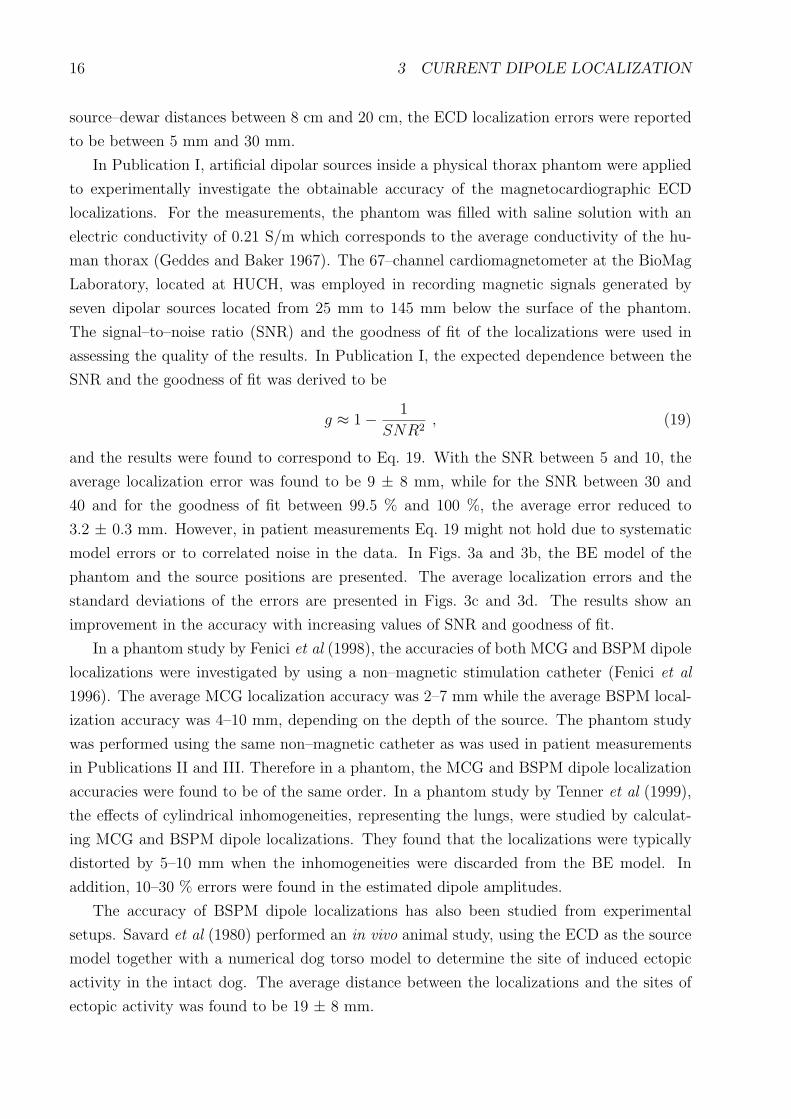
In Publication I, artificial dipolar sources inside a physical thorax phantom were applied

to experimentally investigate the obtainable accuracy of the magnetocardiographic ECD

localizations. For the measurements, the phantom was filled with saline solution with an

electric conductivity of 0.21 S/m which corresponds to the average conductivity of the hu-

man thorax (Geddes and Baker 1967). The 67–channel cardiomagnetometer at the BioMag

Laboratory, located at HUCH, was employed in recording magnetic signals generated by

seven dipolar sources located from 25 mm to 145 mm below the surface of the phantom.

The signal–to–noise ratio (SNR) and the goodness of fit of the localizations were used in

assessing the quality of the results. In Publication I, the expected dependence between the

SNR and the goodness of fit was derived to be

g ≈ 1− 1

SNR2, (19)

and the results were found to correspond to Eq. 19. With the SNR between 5 and 10, the

average localization error was found to be 9 ± 8 mm, while for the SNR between 30 and

40 and for the goodness of fit between 99.5 % and 100 %, the average error reduced to

3.2 ± 0.3 mm. However, in patient measurements Eq. 19 might not hold due to systematic

model errors or to correlated noise in the data. In Figs. 3a and 3b, the BE model of the

phantom and the source positions are presented. The average localization errors and the

standard deviations of the errors are presented in Figs. 3c and 3d. The results show an

improvement in the accuracy with increasing values of SNR and goodness of fit.

In a phantom study by Fenici et al (1998), the accuracies of both MCG and BSPM dipole

localizations were investigated by using a non–magnetic stimulation catheter (Fenici et al

1996). The average MCG localization accuracy was 2–7 mm while the average BSPM local-

ization accuracy was 4–10 mm, depending on the depth of the source. The phantom study

was performed using the same non–magnetic catheter as was used in patient measurements

in Publications II and III. Therefore in a phantom, the MCG and BSPM dipole localization

accuracies were found to be of the same order. In a phantom study by Tenner et al (1999),

the effects of cylindrical inhomogeneities, representing the lungs, were studied by calculat-

ing MCG and BSPM dipole localizations. They found that the localizations were typically

distorted by 5–10 mm when the inhomogeneities were discarded from the BE model. In

addition, 10–30 % errors were found in the estimated dipole amplitudes.

The accuracy of BSPM dipole localizations has also been studied from experimental

setups. Savard et al (1980) performed an in vivo animal study, using the ECD as the source

model together with a numerical dog torso model to determine the site of induced ectopic

activity in the intact dog. The average distance between the localizations and the sites of

ectopic activity was found to be 19 ± 8 mm.

17

(a) (b)

5−10 10−15 15−20 20−30 30−400

2

4

6

8

10

12

14Localisations with SNR better than 5

Signal−to−noise ratio

Loc

alis

atio

n er

ror

/ mm 380

132 61

51 37

Average localisation error Standard deviation of the error

90−95 95−98 98−99 99−99.5 99.5−1000

2

4

6

8

10

12

14Localisations with g better than 90 %

Goodness of fit value / %

Loc

alis

atio

n er

ror

/ mm

255

267

136

104

41

Average localisation error Standard deviation of the error

(c) (d)

Fig. 3: a) The anterior projection and b) the transaxial projection of the BE model of thephantom together with the positions of the seven dipolar current sources. The mean lo-calization errors calculated in certain ranges of c) SNR and d) goodness of fit. Only thelocalizations with the SNR or the goodness of fit belonging to the selected ranges displayed onthe x–axis were included in the calculation. The average errors are plotted by black bars andthe standard deviations of the errors by gray bars. The number of localizations belonging toeach range is displayed on top of the bars. (From Publication I)

18 3 CURRENT DIPOLE LOCALIZATION

3.4 Patient measurements

The ECD has been widely applied in clinical MCG and BSPM source localization studies. In

the following, results from some of these studies are briefly reviewed. Gulrajani et al (1984)

used the ECD to localize the accessory pathway from 26–channel BSPM measurements in

28 WPW–patients. They found that the ECD solutions could not separate the accessory

pathway sites into eight AV locations, however, right–sided, posterior and left–sided pre–

excitation could be separated. Savard et al (1985) calculated ECD localizations from 63

BSPM leads in 14 patients with implanted pacemakers. The localized sites were found to be

within 25 ± 12 mm from the pacing leads.

In MCG studies, Nenonen et al (1991a) used the ECD to localize the pre–excitation sites

in 10 WPW–patients. The MCG measurements were performed with a single–channel de-

vice. They found an average accuracy of 22 ± 10 mm by scaling a standard homogeneous

BE torso model to approximate the true shape of the subjects. Makijarvi et al (1992) ap-

plied the ECD, as well as the quadrupole and the magnetic dipole, in localizing ventricular

pre–excitation sites in 15 WPW–patients. By modeling the volume conductor with an infi-

nite half–space they obtained an accuracy of 73 mm for the ECD, indicating the need for a

more realistic representation of the torso. Weismuller et al (1992) localized accessory path-

ways from 37–channel MCG recordings in seven WPW–patients. In their study, the results

showed an average accuracy of 21 mm with respect to invasive catheter mapping. Nenonen

et al (1993) localized accessory pathways in 12 WPW–patients using a standard homoge-

neous torso model. The average 3D difference between the MCG and the invasive results

was 21 ± 9 mm. Bruder et al (1994a) localized accessory pathways in two WPW–patients,

ectopic activation from two ventricular extrasystoles and two (a shallow and a deep) catheter

positions. An average accuracy of 24 mm was obtained by individual scaling of a standard

homogeneous torso model. Oeff and Burghoff (1994) investigated 18 WPW–patients prior to

catheter ablation and five coronary artery disease (CAD) patients with a sufficient number

of monomorphic ventricular extrasystoles to enable evaluation. The MCG results were com-

pared to the site of successful catheter ablation, and an average difference of 21 ± 17 mm

was found. In the CAD patient group, the origin of the ventricular premature beats was

localized in four patients at the border of infarcted areas. Moshage et al (1996) found an

ECD localization accuracy of 18 ± 5 mm in 19 patients with ventricular arrhythmias with

respect to electrophysiological (EP) mapping. In six patients with a non–magnetic pacing

catheter, the stimulus spike was localized within 12 mm from the position determined from

MR images.

In Publication II, the MCG localization accuracy was investigated in five patients using

a non–magnetic stimulation catheter (Fenici et al 1996). After standard EP studies, the

catheter was placed in four cases in the right ventricle (RV) and in one case in the coro-

19

12

(a) (b)

Fig. 4: a) A triangulated epicardial surface of a patient in Publication II, showing the ECDlocalizations of the tip of the catheter and the cardiac evoked field (1) 3–15 ms and (2) 15–30 ms after the stimulus. b) A transaxial MR image of the heart of the same patient, showingthe localization of the tip of the catheter (gray circle) and the resulting evoked response 3–10 ms later (white circles). (From Publication II)

nary sinus (CS). The position of the catheter was documented in biplane cine X–ray images.

Thereafter, MCG signals were recorded during cardiac pacing in the shielded room of the

BioMag Laboratory. The artificial current dipole in the tip of the catheter stimulates my-

ocardial cells located near to the tip. Therefore, the resulting cardiac activation originates

from the vicinity of the tip. The myocardial activation following a stimulus current pulse

is referred as the myocardial evoked response, which in turn produces a magnetic cardiac

evoked field (CEF). Non–invasive localizations of the tip of the catheter and the myocar-

dial evoked responses were computed from the measured MCG data using patient–specific

homogeneous BE torso models. The mean distance between the tip of the catheter, deter-

mined from fluoroscopy, and MCG localizations during the stimulus spikes was 11 ± 4 mm.

The mean distance between the localizations calculated during the stimulus spikes and in

the beginning of the CEFs was 4 ± 1 mm, as determined from signal–averaged data. The

propagation velocity of the ECDs between 5 ms and 10 ms after the stimuli was found to be

0.9 ± 0.2 m/s. An example of the localization results reported in Publication II is presented

in Fig. 4. The accurate 3D localizations of the tip of the catheter suggest that the MCG

method could be developed towards a useful clinical tool during EP studies.

Only a few studies have been presented with localizations from simultaneous MCG and

BSPM measurements. Bruder et al (1994b) have investigated the accuracy of dipole local-

izations from simultaneously recorded 37–channel MCG and 40–channel BSPM data of two

patients with the WPW syndrome. In their study, the validation was provided by the sites of

20 3 CURRENT DIPOLE LOCALIZATION

successful catheter ablation. The MCG and BSPM accuracies were found to be 20–30 mm.

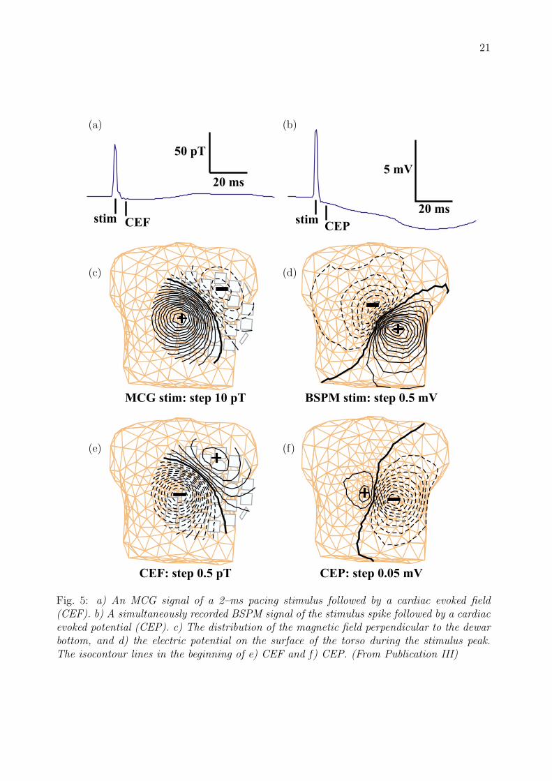
In Publication III, the accuracy of ECD localizations was comprehensively studied for the

first time by using the non–magnetic catheter as a reference current source. The validation

for the localizations was obtained by documenting the position of the tip of the catheter on

biplane fluoroscopic images. Multichannel MCG and BSPM measurements in 10 patients

were then carried out by pacing the heart in the shielded room of the BioMag Laboratory.

The myocardial evoked response reflected as the CEF in the magnetic data and as the car-

diac evoked potential (CEP) in the body surface potential recordings. An example of the

data used in Publication III is presented in Fig. 5. The ECD localizations were calculated

using individual homogeneous and inhomogeneous BE torso models. Using MCG data, an

average 3D localization accuracy of 7–9 mm was obtained which can be considered sufficient

for guiding ablative procedures in a catheterization laboratory. The average BSPM localiza-

tion accuracy obtained in this study was considerably lower, only 25–31 mm. Typically, the

BSPM localization results overestimated the depth of the source.

3.5 Effect of torso modeling

Several studies applying the ECD have been reported concerning the effect of inhomogeneities

in the BE model. Solving the forward problem shows the changes in the morphological pat-

terns of the MCG and BSPM data, due to changing the properties of the volume conductor

model. Horacek et al (1987) assessed how the geometry and the composition of the torso

affect the extracorporal magnetic field, produced by a current dipole in the center of the

ventricular mass. They found that the intraventricular blood masses caused a noticeable

rotation of the maps’ extrema. Both lungs and blood masses tended to swing the distri-

bution towards a field pattern that would have been caused by a dipole oriented along the

anatomical axis of the heart. Purcell et al (1988) found that the outer boundary of the torso

and the intracavitary blood masses had the largest effect on the electric and magnetic field

produced by a single current dipole placed at various locations in the heart. Bruder et al

(1994b) found as well that the outer boundary of the torso had the major influence on both

BSPM and MCG maps, and that the influence of the lungs was smaller than that of the

blood masses.

In the inverse problem studies, Forsman et al (1992) found that the magnetocardiographic

ECD localizations of deep current sources can be distorted even by several centimeters

by discarding the inhomogeneities (lungs, blood masses) from the torso model. Tan et

al (1992) investigated the effect of scaling the torso model and found that by using scaling

factors of 0.9–1.1, the effect on the localization accuracy was typically less than 10 mm

for dipoles tangential to the anterior surface of the torso. For a perpendicular dipole, the

results were affected even by several centimeters. Bruder et al (1994b) also investigated

21

(a) (b)

(c) (d)

(e) (f)

Fig. 5: a) An MCG signal of a 2–ms pacing stimulus followed by a cardiac evoked field(CEF). b) A simultaneously recorded BSPM signal of the stimulus spike followed by a cardiacevoked potential (CEP). c) The distribution of the magnetic field perpendicular to the dewarbottom, and d) the electric potential on the surface of the torso during the stimulus peak.The isocontour lines in the beginning of e) CEF and f) CEP. (From Publication III)

22 3 CURRENT DIPOLE LOCALIZATION

Fig. 6: Elastic deformation of a reference torso model using a deformation grid. In thiscase, both shoulders were raised by 3 cm from their original positions, thus simulating thepositioning differences during the MRI and the MCG measurements. (From Publication IV)

the effect of the torso model on the MCG and BSPM dipole localization accuracies. They

included an anisotropic skeletal muscle layer in the torso model in an approximative manner

and found that the potential on the body surface was smoothed by the anisotropic layer.

This lead to overestimation of the source depth which was more pronounced in the electric

than in the magnetic case. Hren et al (1996) used an inhomogeneous BE model in the

forward computations and discovered that removing the inhomogeneities from the torso

model affected the BSPM localizations slightly less than the MCG localizations. Hren et

al (1998) localized pre–excitation sites along the AV ring from simulated MCG and BSPM

data, and found that using a homogeneous BE model in the inverse calculations caused

average localization errors of 10–15 mm both from the MCG and BSPM data.

In Publication IV, the changes in magnetocardiographic ECD localization results were

evaluated when the geometry and the topology of BE torso models were altered. Individual

thorax models of three patients were built using the segmentation and triangulation methods

developed earlier (Lotjonen et al 1998, Lotjonen et al 1999a). These torso models were serving

as reference models which included the surfaces of the torso, the heart, the lungs and the

cavities. Thereafter, the reference models were modified to represent different aspects of

the BE model generation process. The resulting changes in the localizations were defined

23

by computing the distances from the ECD localizations obtained with the reference models

to the ECD localizations produced by the variated models. Both simulated and measured

multichannel MCG data were used in the calculations. The results showed that the effect

of inhomogeneities (lungs, intraventricular blood) was significant for deep source locations.

However, superficial sources could be localized within a few millimeters even with non–

individual, so–called standard torso models. In general, the thorax model should extend

long enough in the pelvic region, and the positions of the lungs and the ventricles should

be known in order to obtain accurate localizations. An example of an elastic modification

of a reference model used in Publication IV is presented in Fig. 6. The modification was

performed with a deformation grid which allowed, e.g., a realistic simulation of the differences

in the positions of the shoulders during the MR imaging with respect to the MCG recordings.

24 4 EQUIVALENT CURRENT DENSITY

4 Equivalent current density

Magnetocardiographic inverse studies with point–like source models, such as the ECD, are

generally applicable only for sources confined in a small volume of tissue, e.g., at the onset

of the ventricular depolarization. After the onset, the electrical activation spreads in the

myocardium as a wavefront, and the use of point–like source models can no longer be physi-

ologically justified. Therefore, distributed source models provide a more general description

of the current sources in the heart. In the following, the calculation of a distributed current

density, especially applied in biomagnetic inverse studies, will be presented. This source

model consists of dipolar elements with fixed locations. Other distributed source models

used in solving the cardiac inverse problem are the previously mentioned epicardial and

transmembrane potential distributions.

In the literature, the calculation of the equivalent current density was first formulated by

Hamalainen and Ilmoniemi (1984). The calculation of the dipole amplitudes and directions

was based on minimum norm estimation, and the solution was called the minimum norm

estimate (MNE). Consequently, various methods for altering the nature of the solution have

been presented in the literature. In this thesis, the solutions of the cardiomagnetic inverse

problem, approximating the primary current distribution with dipolar elements, are called

minimum norm estimates, or more generally, current density estimates (CDEs).

Solving the inverse problem with a distributed source model, such as the CDE, leads to

an ill–posed problem. The ill–posedness is a mathematical reflection of physical phenom-

ena that include the attenuation and smoothing effects of the volume conductor, and the

measurement noise. Rapid spatial variations in the current distribution inside the heart are

blurred and smoothed in the measured magnetic or electric data. Therefore, a small amount

of perturbation (noise, errors in the volume conductor model, discretization effects etc.) in

the MCG or ECG data tends to be magnified in the inverse solution. The calculation can

be stabilized by using regularization. The regularization produces solutions which may “fit”

worse to the data than the original, unregularized solution but usually are more realistic and

stable. Different regularization schemes applicable in the cardiac inverse problem have been

investigated especially with the epicardial potential distribution (e.g., Messinger–Rapport

and Rudy 1988, Oster and Rudy 1992, Oster and Rudy 1997, Ahmad et al 1998, Brooks et

al 1999), and many of the methods can also be used in calculating CDEs.

4.1 Lead fields

The measured magnetic field values and the primary current distribution can be linked

together via the lead fields Li (Baule and McFee 1970)

Bi(ri) =∫

V ′Li(r

′) · Jp(r′) dv′ , (20)

25

where ri is the location and Bi the magnetic signal detected by the ith sensor. In the

discretization of the problem, the source volume V ′ is replaced by a finite set of source

points r ′k. Thereafter, the sensor lead fields are calculated by placing unit dipoles in x–, y–

and z–directions to each source point r ′k. In the calculation of the lead fields, the properties

of the volume conductor are taken into account. Discretization of Eq. 20 produces a matrix

equation

B = LJ , (21)

where vector Bm×1 contains the magnetic field values, matrix Lm×3n = (L1, · · · ,Lm) is

composed of the lead fields, and vector J3n×1 = (J1x, J1y, J1z, J2x, · · · , Jnz)T contains the

unknown source strengths. The number of observations (sensors) is m while n is the number

of source points. The conventional minimum norm solution of an under–deterministic matrix

equation, such as Eq. 21, can be expressed as

J = L†B = LT (LLT )−1B , (22)

where L† is the pseudo–inverse of L. Eq. 22 relates directly to solution J∗ presented by

Hamalainen and Ilmoniemi (1984, 1994), which is defined as a linear combination of the lead

fields

J∗ =m∑

i=1

ωiLi = ωTL . (23)

The coefficients ωi in Eq. 23 are solved from the magnetic field values using the inner product

matrix Γ (Γij = 〈Li,Lj〉):ω = Γ−1B = (LLT )−1B . (24)

Therefore, the transpose of J∗ equals to the solution in Eq. 22.

In practice, the unknown source strengths J cannot be directly solved from Eq. 22 because

the lead fields of adjacent sensors are nearly linearly dependent on each other. Therefore,

the inner product matrix (LLT ) has a low numerical rank, and the classical solution will be

contaminated by noise. The calculation can be stabilized by using regularization.

4.2 Regularization

In the literature, the truncation of the singular value decomposition (tSVD) (Hamalainen and

Ilmoniemi 1994, Nenonen et al 1994), Tikhonov regularization (e.g., Ferguson and Stroink

1995a) and Wiener regularization (Numminen et al 1995) have been used in stabilizing the

calculation of the current density estimates. In addition, different iterative, temporal and

statistical regularization methods, mostly related to the calculation of the epicardial potential

distribution, have been presented. In the following, these methods are briefly reviewed.

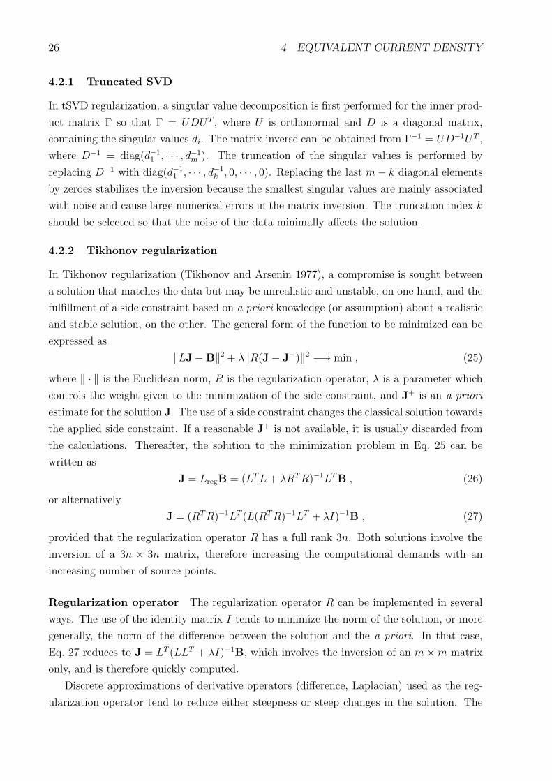
26 4 EQUIVALENT CURRENT DENSITY

4.2.1 Truncated SVD

In tSVD regularization, a singular value decomposition is first performed for the inner prod-

uct matrix Γ so that Γ = UDUT , where U is orthonormal and D is a diagonal matrix,

containing the singular values di. The matrix inverse can be obtained from Γ−1 = UD−1UT ,

where D−1 = diag(d−11 , · · · , d−1

m ). The truncation of the singular values is performed by

replacing D−1 with diag(d−11 , · · · , d−1

k , 0, · · · , 0). Replacing the last m − k diagonal elements

by zeroes stabilizes the inversion because the smallest singular values are mainly associated

with noise and cause large numerical errors in the matrix inversion. The truncation index k

should be selected so that the noise of the data minimally affects the solution.

4.2.2 Tikhonov regularization

In Tikhonov regularization (Tikhonov and Arsenin 1977), a compromise is sought between

a solution that matches the data but may be unrealistic and unstable, on one hand, and the

fulfillment of a side constraint based on a priori knowledge (or assumption) about a realistic

and stable solution, on the other. The general form of the function to be minimized can be

expressed as

‖LJ−B‖2 + λ‖R(J− J+)‖2 −→ min , (25)

where ‖ · ‖ is the Euclidean norm, R is the regularization operator, λ is a parameter which

controls the weight given to the minimization of the side constraint, and J+ is an a priori

estimate for the solution J. The use of a side constraint changes the classical solution towards

the applied side constraint. If a reasonable J+ is not available, it is usually discarded from

the calculations. Thereafter, the solution to the minimization problem in Eq. 25 can be

written as

J = LregB = (LTL+ λRTR)−1LTB , (26)

or alternatively

J = (RTR)−1LT (L(RTR)−1LT + λI)−1B , (27)

provided that the regularization operator R has a full rank 3n. Both solutions involve the

inversion of a 3n × 3n matrix, therefore increasing the computational demands with an

increasing number of source points.

Regularization operator The regularization operator R can be implemented in several

ways. The use of the identity matrix I tends to minimize the norm of the solution, or more

generally, the norm of the difference between the solution and the a priori. In that case,

Eq. 27 reduces to J = LT (LLT + λI)−1B, which involves the inversion of an m × m matrix

only, and is therefore quickly computed.

Discrete approximations of derivative operators (difference, Laplacian) used as the reg-

ularization operator tend to reduce either steepness or steep changes in the solution. The

27

discrete surface Laplacian operator ∆ can be constructed, e.g., by using one of the approxi-

mations presented by Huiskamp (1991). In the simplest approximation, the Laplacian of a

general function f is formulated for a regular plane grid:

∆f0 ≈ CN∑

i=1

(fi − f0) , (28)

where f0 is the value of the function in the central point, fi are the values in theN neighboring

grid points, and C is a constant depending on N and on the distance between the central

and the neighboring points. In a regular grid, the neighboring points are spaced at equal

angles with a constant distance from the central point. Therefore, Eq. 28 is valid, e.g., for a

grid consisting of equilateral triangles. In a more general case, such as on the triangulated

surface of the heart, the distances and the spacing angles of the neighboring grid points

need to be taken into account in the Laplacian. However, the crude approximation given by

Eq. 28 has been found to be sufficient with respect to a more accurate formulation in the

regularization of uniform double layer solutions on the ventricular surface (Huiskamp 1991).

In Publication VI, realistic surfaces of the torso and the left ventricle (LV) were used

to test the zero– and second–order regularization of CDEs calculated from simulated, dis-

tributed current sources located on the surface of the LV. The simulated MCG data also

contained a realistic amount of measurement noise. For deeper source locations, the zero–

order regularization was found to shift the estimates towards the anterior surface of the LV.

With second–order regularization, the estimates were correctly centered with respect to the

known source region. An example of the comparison between the regularization operators,

carried out for a deep source location, is presented in Fig. 7.

Selecting a value for λ In the literature, numerous methods have been presented for

selecting a proper value for the regularization parameter λ. These methods include, e.g., the

discrepancy technique (Morozov 1984), the generalized cross–validation (Golub et al 1979),

and the L–curve method (Hansen 1992). More recently, a technique based on zero–crossing

of the function in Eq. 25 has been presented (Johnston and Gulrajani 1997). The L–curve

method, also applied in this thesis, has been most widely used in the regularization of the

biomagnetic inverse problem.

A numerical algorithm to compute an optimal value of λ by using the L–curve method

has been presented by Hansen and O’Leary (1993). With the L–curve, a balance between the

minimization of the residual and the side constraint in Eq. 25 can be found as the value of λ

is varied. The name of the method relates to the shape of a continuous curve C0 : ‖LJ −B‖, ‖RJ‖. In the over–determined case of solving the epicardial potential distribution from

body surface potentials, the L–curve method has been formulated by Clements et al (1994).

By using the generalized singular value decomposition of the matrices L = UCX−1 and R =

V SX−1, the regularizing matrix Lreg in Eq. 26 can be written as X(CTC + λSTS)−1CTUT

28 4 EQUIVALENT CURRENT DENSITY

R = I

R = D2

Anterior view Transaxial view

A

A

B

B

A

A

B

B

oo

o

oo o

o

oo

o

o oo

oo o

oo

o

oo o

o

oo

o

o oo

oo o

Fig. 7: CDEs calculated for a distributed current source, located on the posterior surface of theLV, using zero–order (upper row) and second–order (bottom row) Tikhonov regularization.The actual positions of the dipoles used in generating the data are marked with black circles.The amplitude of CDEs is coded with grayscale values; darkest gray indicates largest currentdensity (A = apex, B = base). (From Publication VI)

(Clements et al 1994). In the decomposition, U and V are orthonormal, and X is non–

singular. If L is assumed to have full rank m and R is assumed to have full rank 3n, the

matrices C and S for the under–deterministic case in Eq. 21 are of the form

C = (Om×(3n−m) Cm ) , S =(

I3n−m O(3n−m)×m

Om×(3n−m) Sm

),

where Cm = diag(α1, · · · , αm) and Sm = diag(β1, · · · , βm). The generalized singular values

of matrices L and R are defined as µi =αi

βi. Therefore, the regularized solution J in Eq. 26

can be expressed as

J =m∑

i=1

1

βi

µi

µ2i + λ

〈ui,B〉x3n−m+i , (29)

where ui refers to the ith column of U and x3n−m+i to the (3n − m + i)th column of X. By

using the expression in Eq. 29, the squared norm of the residual can be written as

‖LJ−B‖2 =m∑

i=1

[λ

µ2i + λ

〈ui,B〉]2

, (30)

29

λ gets smaller

λ gets larger

ln || RJ ||

ln || LJ - B ||

Fig. 8: A schematic presentation of the shape of the L–curve.

and the squared norm of the side constraint is

‖RJ‖2 =m∑

i=1

[µi

µ2i + λ

〈ui,B〉]2

. (31)

Eqs. 30 and 31 again coincide with the results presented by Clements et al (1994). It can

be seen that as the value of λ is increased, the norm of the residual is increasing while the

norm of the side constraint is decreasing. The opposite is true for decreasing λ values.

The L–curve is usually plotted on a log–log scale. By defining the functions x(λ) and

y(λ) as

x(λ) =1

2ln

m∑

i=1

[λ

µ2i + λ

〈ui,B〉]2

, (32)

y(λ) =1

2ln

m∑

i=1

[µi

µ2i + λ

〈ui,B〉]2

, (33)

the value of the residual can be plotted as a function of the side constraint with varying λ.

A schematic illustration of the shape of the curve is presented in Fig. 8. The goal is to find

a value for λ which balances the minimization between the residual and the side constraint

at the “corner” point of the L–curve. The corner is defined to have a maximal curvature. A

mathematical expression for the curvature can be obtained from

κ(λ) =x′(λ)y′′(λ)− y′(λ)x′′(λ)((x′(λ))2 + (y′(λ))2)3/2

. (34)

The first and second order derivatives of functions x(λ) and y(λ) with respect to λ have been

formulated in Publication V in the case R = I. However, the formulations also hold for a

30 4 EQUIVALENT CURRENT DENSITY

more general choice of R if the singular values in the formulas of Publication V are replaced

with the generalized singular values µi.

For the existence of the corner point of the L–curve, Hansen (1992) has presented con-

ditions which include, e.g., that the noise in the measured data is randomly distributed and

has a zero mean, and that the amplitude of the noise is smaller than the amplitude of the

signal. Especially the former condition might not be satisfied because correlated noise can

be present in the measured data. Also the reduction of the signal amplitude tends to dis-

tort the shape of the L–curve. Therefore with measured data, the curvature function given

in Eq. 34 sometimes results in multiple maxima, and the corner point cannot be uniquely

defined. However, a reasonable value for λ can be obtained by inspecting the quality of the

calculated CDEs.

4.3 Weighted solutions

A scheme for weighting, or pre–conditioning of the lead field matrix has been proposed by

Ferguson et al (1995b) by adding a diagonal matrix D into the original matrix formulation

of Eq. 21:

B = LDD−1J . (35)

Thus, the original equation does not change due to the addition of the weighting matrix D.

In D, possible a priori information about the solution can be used. If the product of matrices

L and D is denoted as L, the solution of the under–determined Eq. 35 can be written as

(Ferguson et al 1995b)

J = D[LT (LLT )−1B] . (36)

Although the original equation does not change due to the addition of the weighting matrix,

the solution of Eq. 36 changes. Ferguson et al (1995b) proposed the matrix D to be diagonal,

and the diagonal elements to equal to the square roots of the best–fitting dipole strength

at each of the source locations. They found that with simulated data, the pre–conditioning

of the lead field matrix improved the quality of the solutions with respect to the tSVD

and Tikhonov regularized solutions. The pre–conditioning tends to favor deeper solutions

as the weights for deeper sources will be larger than those of the shallow sources. Despite

the addition of the weighting matrix D, the matrix to be inverted in Eq. 36 is close to

singular. The truncation of the SVD or Tikhonov regularization can be used in balancing

the computation of the weighted solutions.

The weighting of the solution can also be applied iteratively. A method for iterative

weighting, termed as the FOCUSS algorithm, was suggested by Gorodnitsky et al (1995).

In this approach, the elements of the weighting matrix D are updated using the information

obtained during previous iterations. Gorodnitsky et al (1995) suggested to initialize D with

the identity matrix. In the following iterations, they proposed that the elements of D would

31

be obtained from the components of the current distribution calculated during the previous

iterations:

Dk =

Jk−11,x 0

. . .

0 Jk−1n,z

, (37)

where Jk−1i,j is the jth component of a dipole located in the ith source point calculated during

the k−1th iteration. Alternatively, information about all the previous solutions can be added

to the weighting matrix:

Dk = Dk−1 ·

Jk−11,x 0

. . .

0 Jk−1n,z

. (38)

The iterations are continued until the magnitudes of the changes in the solution are below

a pre–set limit.

The truncated SVD, the zero–order Tikhonov regularization, the weighting and the iter-

ative weighting approaches were tested in Publication V by using measured MCG data. The

weighting matrix D was initialized with the square roots of the optimal dipole strengths. The

measurements were carried out with a non–magnetic catheter in the heart, thus providing

an exact validation for the location of the current source. It was found that when the source

was located relatively close to the sensors, all regularization techniques were able to localize

the center point of the source region. However, for a deeper source location, weighting was

required to produce a correct estimate of the underlying current distribution.

Another iterative approach has been suggested by Tilg et al (1995) where the number

of the reconstruction points was reduced by removing the point with the smallest dipole

amplitude in the subsequent step of iteration. The iterations were terminated at a prescribed

number of source points. The method was found to localize both focal and distributed sources

from simulated MCG data. However, the number of the source points to be included in the

final solution might be difficult to determine with measured MCG data (Tilg et al 1995).

4.4 Temporal and statistical regularization

In addition to the one time point –approach described above, temporal information can be

used in the regularization process. This has been proposed, e.g., by Oster and Rudy (1992)

who found a marked improvement in the inversively reconstructed epicardial potential dis-

tribution when information from previous time instants were incorporated in the calculation.

Spatial characteristics of the measured data can also be taken into account. Oster and Rudy

(1997) suggested a regional regularization approach in reconstructing the epicardial poten-

tial distribution. In their method, the amount of regularization was adjusted according to

the spatial characteristics of body surface potential maps. The method was found to im-

prove the epicardial potential reconstruction with respect to global regularization where the

32 4 EQUIVALENT CURRENT DENSITY

amount of regularization was controlled with one parameter only. In addition, Brooks et al

(1999) used multiple constraints (both spatial and temporal) in Tikhonov–type regulariza-

tion and presented a so–called L–surface method for selecting values for the regularization

parameters.

Among the statistical regularization schemes proposed, the incorporation of the spatial

covariance in solving the epicardial potential distribution was first suggested by Martin et al

(1975). Recently, the method has been studied by van Oosterom (1999). In this approach,

the solution is formulated as the maximum–a–posteriori estimate which incorporates the

spatial covariances of the epicardial potential distribution and the noise. Van Oosterom

(1999) found that the inverse solution was more robust with respect to perturbations (noise,

inhomogeneities) than the solutions obtained with zero– and second–order Tikhonov regu-

larization. Sekihara and Scholz (1996) used a generalized Wiener estimation technique and

found that the method could reconstruct 3D current distributions in case of simulated data.

4.5 Applications of CDE

4.5.1 Ischemia studies

One of the most interesting areas in clinical MCG today is the detection and characteri-

zation of myocardial ischemia and viability. A new and accurate non–invasive method for

recognition of ischemia would have important clinical applications, especially because novel

therapeutic interventions for revascularization (e.g., coronary angioplasty and transmyocar-

dial laser) are emerging. An acute ischemia changes the shape of the action potential of

myocardial cells. The mechanisms causing the changes have been investigated, e.g., by

Shaw and Rudy (1997a, 1997b). Typically, the value of the resting potential is increased in

ischemic cardiac cells, whereas during the plateau phase (see Fig. 1) the value of the mem-

brane potential is decreased with respect to the monophasic action potential of a healthy

cell. Such changes lead to an injury current which in the resting state flows from the ischemic

area into the healthy myocardium, and in the opposite direction during the repolarization.

In MCG recordings, the ischemia reflects as changes (elevations or depressions) during the

ST–segment (e.g., Cohen et al 1971, 1983, and Savard et al 1983).

Infarcted and ischemic regions have been simulated, e.g., by Czapski et al (1998) who

compared the isocontour maps of anterior and inferior myocardial infarction (MI) to the ones

produced by a healthy heart. They found that the isocontours of the difference maps more or

less maintained their pattern throughout the depolarization. To investigate the applicability

of the CDE in localizing ischemia from MCG measurements, Killmann et al (1995) used a

computer model of the human heart to simulate the excitation and repolarization processes

in different cases of myocardial ischemia. The CDE was applied at the S–point of the QRS–

complex in a plane positioned 7–10 cm below the simulated MCG measurement grid. The

33

Ant

Sep

Pos

Lat

CDEamplitude

Max

Min

Fig. 9: CDEs for two RCA patients (upper row) and for two LAD patients (bottom row),visualized with polar maps (Ant = anterior, Lat = lateral, Pos = posterior, and Sep = septalregion). The amplitudes of the CDEs for each patient are coded with grayscale values. (FromPublication VI)

direction of the dipolar elements in CDE and the position of the largest elements were found

to reflect the location of the ischemic area.

In Publication VI, CDE was applied on the epicardial surface of the LV in 13 CAD

patients. In the MCG measurements, exercise testing was used as described by Takala

(1999) to induce acute ischemia in the cardiac tissue. The individual torso and LV surfaces

were constructed from MR images. The current density estimates were calculated from

the ST–segment exercise–rest difference signals using second–order Tikhonov regularization.

The calculated CDEs were compared to the clinical reference information about the LV

function. In four patients with a single–vessel CAD, an increase in the CDE amplitude was

found to correlate with the expected ischemic myocardial regions, supplied by the stenotic

coronary artery. The CDEs of the single–vessel CAD patients are shown in Fig. 9 as polar

map presentations. In the polar maps, the apex of the heart is projected at the center. The

map can roughly be divided into four regions according to the coronary anatomy: anterior,

lateral, posterior, and septal regions. In the two patients with a stenosis in the right coronary

artery (RCA), an increase in the CDE amplitude is detected in the posterior region of the LV

which corresponds to the expected ischemic myocardial regions in patients with a stenosis in

the RCA. In the two patients with a stenosis in the left anterior descending (LAD) coronary

34 4 EQUIVALENT CURRENT DENSITY

(a) (b)

Fig. 10: a) The PET result of a three–vessel CAD patient showing a scar in the lateral region(dark area). b) The CDE corresponding to the PET result in (a) together with the division ofthe polar map into 24 segments. The darkest gray indicates highest CDE amplitude. (FromPublication VI)

artery, the CDEs are focused in the apex, in the anterior and in the septal regions of the

LV, thus matching to the myocardial regions supplied by the LAD.

Nine of the patients in Publication VI had three–vessel CAD with regional or global LV

dysfunction caused by severe chronic myocardial ischemia, previous MI or both. In this

patient group, positron emission tomography (PET) images were used to separate the areas

of viable myocardial tissue from the scar regions. Also in this patient group, the CDEs were

calculated from the ST–segment exercise–rest difference signals. The analysis of the CDEs

was based on the fact that no current should build up in MI scar regions. The calculated

CDEs were compared to the PET data by dividing the polar map of the LV into eight

sectors: two anterior, two lateral, two septal, and two posterior sectors. Each sector was

further divided into three short axis planes: apex, middle, and base. Thus, the comparison

was carried out in 24 segments which, by PET, were determined to be either viable tissue or

scar. The scale of the CDEs was divided to indicate low and high CDE amplitude. Therefore,

a match was obtained if a low CDE amplitude was detected in a scar segment, or a high

CDE amplitude in a viable segment.

An example of the comparison between PET and CDE carried out in Publication VI

is presented in Fig. 10. The PET result indicates a lateral scar area which is shown as a

dark region. The anteroseptal, septal and posteroseptal regions indicate viable myocardium.

The corresponding CDE shows an increased amplitude in the anteroseptal, septal and pos-

teroseptal regions, thus matching well with the PET data. A decreased CDE amplitude is

35

observed in the lateral region which was found to be a scar area.

The overall results of the comparison between PET data and calculated CDEs for all

nine three–vessel CAD patients showed an average match of 77 % between the segments

of high and low amplitude in CDEs, and the viable and scar areas in PET, respectively.

Therefore, the classification (scar or viable tissue) obtained from the calculated CDEs was

correct in approximately 18/24 segments. In Publication VI, the CDE was thus found to be

a potential method for localizing both myocardial ischemia in single–vessel CAD patients,

as well as more complex forms of ischemia in three–vessel CAD patients.

In addition to MCG studies, ischemic regions have also been localized from multichannel

BSPM measurements by solving the epicardial potential distribution (MacLeod et al 1995).

In this study, seven patients underwent percutaneous transluminal coronary angioplasty

(PTCA) where the balloon inflations produced acute transient ischemia. The estimated

ischemic regions, determined from the calculated epicardial potential distributions, were

compared to a qualitative estimate of the perfusion region based on fluoroscopic examination

of each patient’s coronary anatomy and PTCA balloon location. It was found that the

ischemic regions, predicted by the epicardial potential distributions, included the perfusion

zone determined fluoroscopically.

4.5.2 Other clinical studies

The CDE was applied by Leder et al (1998) in two MI patients and in two healthy sub-

jects. Current density estimates were calculated on the surface of the left ventricle during

ventricular depolarization to detect a decreased current amplitude in the MI patients. Low

regional and global current densities were found in the MI patients. Regions of low current

density were found to correspond to infarcted segments. The CDEs of the healthy subjects

displayed less marked areas of low current density.

The origin site of a malignant ventricular tachycardia (VT) has also been localized with

current density estimation (Muller et al 1999). The CDE was calculated on the surface

of the left ventricle. The origin site of the VT, determined from the X–ray images of the

ablation catheter position during EP studies, was used as the gold standard. The area with

the highest current density in the CDE was then compared to the gold standard. It was

found that the CDE localized the origin of the VT within 10 mm.

36 5 UNIFORM DOUBLE LAYER

5 Uniform double layer

The activation sequence on the ventricular surface, including both epi– and endocardium,

can be estimated from BSPM and/or MCG data with the uniform double layer (UDL) source

model. This spatio–temporal model consists of elementary double layer current sources of

equal strength. The direction of the double layer sources is perpendicular to the surface,

and they are oriented inwards in the cardiac muscle. The parameters of the model are the

activation times of each double layer element during the ventricular depolarization phase.

The justification of the model can be derived from the bidomain model in the sense that

if equal anisotropy ratios in the intra– and extracellular domains are assumed, the volume

distribution of cardiac sources can be replaced by an appropriate double layer on the surface

of the heart. Calculation methods required in finding an UDL based inverse solution have

been developed, e.g., at the University of Nijmegen in the Netherlands (Huiskamp and van

Oosterom 1988). Previously, UDL based inverse solutions have been calculated mainly from

BSPM recordings. Solving the cardiac inverse problem with the UDL model has been found

to be less ill–posed than using the epicardial potential distribution as the source model, and

very promising results have been obtained (e.g., Tilg et al 1997). However, until recently,

the quality of UDL based inverse solutions has been evaluated with invasive data only in a

small number of situations. In this thesis, invasively recorded epicardial potential data were

used as a reference in estimating the quality of epicardial activation times calculated from

both BSPM and MCG recordings.

5.1 Formulation of the UDL model

In the UDL model, the magnetic field or the electric potential is considered to be generated

by double layer (dipolar) current source elements located on the ventricular surface S ′. The

mapping between the current source elements and the field values is described by a (magnetic

or electric) transfer function A(r, r ′) and by the ventricular activation times τ(r ′). Once the

activation wavefront has reached the point r ′ (at time τ(r ′)), the point remains activated

throughout the whole depolarization sequence. The basic equation for the UDL model is

F (r, t) =∫

S′A(r, r ′)H(t − τ(r ′)) dS ′ (39)

where F (r, t) denotes either to the measured component of the magnetic field or to the

electric potential in point r at time t. H(t− τ(r ′)) is the Heaviside step function accounting

for the fact that the elementary source at r ′, once switched on at time τ(r ′), remains on until

the whole ventricular surface S ′ has been activated (Huiskamp and van Oosterom 1988).

The inverse problem now consists of finding the unknown activation times τ(r ′) in the

activation time interval [0, T ] when the magnetic field or potential values F (r, t) on the

measuring surface S are known. The activation times can be obtained by solving the following

37

minimization problem:

∫ T

0

∫S

(∫S′

A(r, r ′)H(t − τ(r ′)) dS ′ − F (r, t))2

dS dt −→ min . (40)

In the discretization of Eqs. 39 and 40, the finite extent of the elementary sources on the

ventricular surface needs to be taken into account. This can be achieved by smoothing the

Heaviside step function H(t− τ(r ′)) in a suitable way (Huiskamp and van Oosterom 1988).

Solving the activation times is also an ill–posed problem in the sense that small changes

in F (r, t) may cause large variations in τ(r ′). Therefore, regularization methods are again

needed to stabilize the calculation. Within the UDL model, Tikhonov regularization with the

surface Laplacian (Huiskamp 1991) as the regularization operator R is usually used, because

it can be assumed that there are no sudden changes in the activation times of adjacent points

on the ventricular surface. The discretized and regularized minimization problem related to

Eq. 40 then states:

‖AΥwτ − F‖2 + λ‖Rτ‖2 −→ min , (41)

where Υwτ contains the smoothed activation times τ . The smoothing of the Heaviside step

function is controlled with the parameter w (Huiskamp and van Oosterom 1988) while the

amount of regularization is again controlled with the parameter λ.

The minimization of Eq. 41 is carried out with a quasi–Newton optimization algorithm,

which iteratively finds better solutions τ that minimize Eq. 41. In the algorithm, an initial

estimate for the activation times is needed. The quality of the initial estimate should be as

high as possible in order to prevent the minimization algorithm from converging into local

minima. There are at least two ways of calculating the initial estimate. In the first approach,

an integration over the QRS–complex is performed for Eq. 39:

∫ T

0F (r, t) dt =

∫ T

0

[∫S′

A(r, r ′)H(t − τ(r ′)) dS ′]

dt , (42)

where the left–hand side can be reduced into the summation of the magnetic field or the

potential values at the observation point r, and the right–hand side effectively contains the

values of the transfer matrix A multiplied by the activation times τ . With the definition

f(r) ≡ ∫ T0 F (r, t) dt, a discretized version of Eq. 42 can be expressed as

f = Aτ . (43)

The initial estimate for τ is then obtained by multiplying the integrated (summed) field

values f with the (regularized) pseudoinverse of A. In the regularization, truncated SVD

was applied by Huiskamp and van Oosterom (1988).

In a more recent approach for calculating the initial estimate for τ , Huiskamp and Green-

site (1997) used the so–called critical point theorem. In the method, the SVD of the signal

matrix F is first calculated: F = UDV T where U and V are orthonormal matrices. The

38 5 UNIFORM DOUBLE LAYER

matrix D is composed of a diagonal matrix, containing the singular values of F , and a zero

matrix. In the case of measured data, from a certain rank reff onward the singular values

will be dominated by noise. This rank is considered to be the effective rank of F , which

separates the signals generated by the current sources in the heart and the measurement

noise. If the rank reff is known, the first reff rows of U can be considered to span the spatial

signal space. The remaining rows of U are assumed to span the noise space. The rows of V

are said to span the temporal signal and noise spaces.

The construction of the spatial signal space is required in the formulation of the critical

point theorem. The critical points r ′cr of the surface activation function τ are its extremal

points where |∇τ(r ′cr)| = 0. The critical point theorem, formulated by Greensite (1995),

states that r ′cr is a critical point of τ if, and only if, the transfer vector A(·, r ′

cr) associated

with this point is contained in the spatial signal space. This theorem can be utilized by

gradually constructing the spatial signal space and by calculating the distances between the

transfer vectors A(·, r ′) and the signal space. Huiskamp and Greensite (1997) defined the

following distance function

M t0(r

′) =

∣∣∣∣∣1−reff∑i=1

〈a(·, r ′),ui〉2∣∣∣∣∣−1

, (44)

where a(·, r ′) = A(·, r ′)/‖A(·, r ′)‖ is the normalized transfer function, 〈·, ·〉 denotes the

inner product in the signal space, and ui is the ith spatial eigenvector resulting from the

SVD of the signal matrix F constrained to the time interval [0, t]. The function M t0(r

′) will

tend to infinity for a critical point r ′cr when t reaches the critical time tcr = τ(r ′

cr). Because

the separation between the signal and noise spaces is more inaccurate for small values of t

than for larger values, Huiskamp and Greensite (1997) introduced two distance functions:

M+(r ′, t) ≡ M t0(r

′) and M−(r ′, t) ≡ MTt (r

′) , 0 ≤ t ≤ T . The properties of M−(r ′, t) will

be opposite to M+(r ′, t) in the sense that for a critical point, the value of M−(r ′, t) will be

initially high and experience a sudden drop to a small value at the critical time tcr. Also

M−(r ′, t) will be more accurate for critical points occurring at early stages of activation.

Finally, the functions M+(r ′, t) are M−(r ′, t) can be combined into a third function:

Z(r ′, t) ≡ M+(r ′, t)− M−(r ′, t) which for a critical point will show a zero crossing accom-

panied by a large positive jump at it’s critical time. Huiskamp and Greensite (1997) also

found that even for a non–critical point, a zero–crossing in Z(r ′, t) is observed, although

the amplitude of the positive jump is much smaller. As the function Z(r ′, t) was found to

behave like an activation wavefront, an isochrone representation of the zero–crossing times

can be made. The reconstructions of zero–crossing times, with correct locations of extremal

points, have been used in this thesis as initial estimates for the quasi–Newton algorithm.

39

5.2 Clinical studies

The UDL model is suitable for describing the ventricular activation which propagates as an

activation wavefront in a structurally healthy heart. Huiskamp and van Oosterom (1988)

calculated the activation sequences with individual BE torso models for three healthy sub-

jects and compared the results with an experimentally documented ventricular activation

sequence (Durrer et al 1970). The reference sequence shows initial activation in the left

ventricular endocardium, secondary activation in the right ventricular endocardium, early

epicardial breakthrough in the anterior part of the right ventricle, and secondary break-

through in the anterior part of the left ventricle. The latest activation takes place in the

posterobasal area of the right ventricle. The activation time maps calculated by Huiskamp

and van Oosterom (1988) showed reasonable agreement with the known activation sequence.

Oostendorp et al (1996) used multichannel MCG and BSPM data recorded in the same

patient and calculated the activation times from both datasets. In general, the solutions

showed similar features with the root–mean–square (RMS) difference of 6.1 ms. In addition

to measured data, Tilg et al (1997) also generated simulated MCG and BSPM data for one

subject. The relative differences in the activation time maps were 10 % and 15 % for the

simulated and measured MCG and BSPM data, respectively.

Until recently, only few validation studies with the UDL model using invasively recorded

data have been reported. Huiskamp et al (1992) found that the UDL model correctly lo-

calized the site of earliest activation from paced BSPM data, obtained from catheterized

patients. Oostendorp et al (1997) used measured epicardial activation times from a dog

heart suspended in a torso shaped tank. In this experiment, the correspondence between the

measured and the computed activation times was good, showing an RMS difference of only

4 ms at the epicardial electrodes. In a recent validation study, Tilg et al (1999) used inva-

sive human data recorded with an electroanatomical catheter mapping system (CARTOTM,

Biosense, Ltd.). The invasive mapping system enables potential measurements together with

information about the recording site. The invasively measured endocardial AT map of the

right ventricle was compared to the calculated endocardial activation times, obtained from

62–channel BSPM data. The results were in good qualitative agreement, and the correlation

coefficient for the measured and calculated activation times was found to be 0.84.

In Publications VII and VIII, the UDL model has been used in calculating activation

times in four patients from 67–channel MCG and 123–channel BSPM recordings. In the

validation of the results, invasively measured epicardial electrograms were used to construct

the reference epicardial activation times. The invasive data were recorded during arrhythmia

surgery from the epicardial surfaces of the patients with a 102–channel socket electrode

system (CardioLabR Prucka Engineering, Inc., Houston, TX, USA). Based on MR images,

an individual BE torso model was constructed for each patient, including the torso boundary,

40 5 UNIFORM DOUBLE LAYER

the lungs, and the cavities within the heart. The ventricular surface, including both epi–

and endocardium, was also reconstructed from the MR images. An algorithm was developed

which allowed the mapping of the invasive data on the epicardial surface of the heart. The

algorithm simulated the positioning of the electrode sock around the heart on basis of a sketch

made during surgery. In Publication VII, the activation times computed from the BSPM

recordings were compared to the invasive data. Publication VIII presents a comparison

between the activation times produced from MCG and BSPM data, and the invasive data.

The overall patterns of activation in the reference data were reproduced relatively well in

the activation time maps computed from MCG and BSPM data. However, precise locations

for the early and late activation spots could not be found from the calculated activation

time maps. All patients included in Publications VII and VIII had previously suffered

from myocardial infarctions. The UDL model is based on the assumption of a uniform

source strength surrounding the whole ventricular muscle. This assumption is not valid for

infarcted regions, which, no doubt, cause some of the differences found between the measured

and computed activation times. In addition, the uncertainty of approximately 1–2 cm in the

epicardial electrode locations likely affects the comparison between the measured and the

calculated activation times.

In Fig. 11, an example of the measured and the calculated activation times on the epi-

cardial surface of the heart is presented. The isocontours of the activation times are shown

with a step of 5 ms. The measured activation times have been interpolated between the

epicardial electrode locations. The activation time map generated from the measured data

shows an early spot on the anterior surface of the RV. Another site of early activation is

found in the latero–basal region of the LV. Late activation is detected in the apical region.

In the activation time map calculated from BSPM data, early activation is detected on the

anterior surface of the RV, and also in the apical region. Late activation is found between

the two sites of early activation, and in the basal regions of the LV. In the activation times

computed from MCG data, early activation is located on the anterior surface of the RV, as

well as in the lateral and postero–basal regions of the LV. Late activation is detected in the

apical region. Therefore, in the MCG based UDL solution, the overall pattern of activation is

reproduced relatively well while in the BSPM solution, the activation pattern on the anterior

surface of the RV is somewhat shifted with respect to the measured data.

41

45

70

50

80

45

50

60

65

55

65

6050

45

40

5550

60

70

65

45

40

25

75

40

35

85

70

60

65

55

75 80

50

70

55

40

50

60

(a)

(b)

(c)

Fig. 11: An example of the comparison between a) the measured, b) the calculated BSPMand c) the calculated MCG activation times, presented on an anterior and on a posteriorprojection of the ventricular epicardial surface. The lightest and darkest gray indicate earliestand latest activation, respectively. The activation times are shown in milliseconds. Thelocations of the epicardial electrodes are marked with circles.

42 6 CARDIOMAGNETIC INSTRUMENTATION

6 Cardiomagnetic instrumentation

In the following, the multichannel instrumentation used in cardiomagnetic studies is briefly

described. The main focus is on the BioMag Laboratory, where all the magnetic measure-

ments used in this thesis were performed. A comprehensive list of multichannel SQUID

devices currently employed in biomagnetic studies (brain and heart) has recently been pre-

sented by Nowak (1998).

6.1 BioMag Laboratory

The BioMag Laboratory at HUCH, founded in 1995, has state–of–the–art facilities both for

basic research and for clinical applications in functional bioelectromagnetic cardiac and brain

studies. In a three–layer high–performance magnetically shielded room, providing shielding

against ambient urban magnetic noise (Paavola et al 2000), a 122–channel neuromagnetome-

ter (Knuutila et al 1993) and a 67–channel cardiomagnetometer have been installed. An

outer view of the shielded room is presented in Fig. 12a. In addition, a 64–channel bioelec-

tric recording system designed for simultaneous use with biomagnetic recordings (Virtanen

et al 1997), a 128–channel portable BSPM system (Simelius 1998), modern imaging facili-

ties in HUCH, including anatomical and functional MRI, and a fast asynchronous transfer

mode (ATM) network in the hospital and between the Finnish universities, give a unique

framework for the studies.

The 67–channel cardiomagnetometer was designed and constructed in collaboration be-

tween Neuromag Ltd., Helsinki, and the Laboratory of Biomedical Engineering at Helsinki

University of Technology (Montonen et al 2000). The cardiomagnetometer is presented in

Fig. 12b. The sensor array consist of seven axial and 60 planar DC (direct current) SQUID

gradiometers in a hexagonal grid. The channel layout is presented in Fig. 13. The func-

tioning of SQUID detectors will not be handled here; it has been described in detail, e.g.,

by Katila (1989). The wire–wound axial first–order gradiometers have a baseline of 80 mm;

the pick–up coil radius is 37.5 mm. The thin–film planar gradiometers have a baseline of

16.2 mm, and they are arranged in 30 units which consist of two perpendicular figure–of–eight

loops. The magnetic field component perpendicular to the surface of a sensor is described

by Bz. The axial gradiometers measure the change in Bz along the surface normal of the

sensor (∂Bz/∂z), while the planar gradiometers measure the change in Bz parallel to the

sensor surface (∂Bz/∂x and ∂Bz/∂y). Four planar units, located at the edge of the array,

are positioned perpendicularly to the dewar bottom, while the other 26 units are parallel

to the bottom. The system is modular in the sense that the axial and planar gradiometers

are interchangeable. High sensitivity of the gradiometers was reached by minimizing the

magnetic noise caused by the conducting materials inside the measurement dewar (Nenonen

et al 1996); the noise levels are about 3 fT/√Hz for axial and 3 fT/cm

√Hz for planar sensors

43

(a) (b)

Fig. 12: a) The magnetically shielded room and b) the 67–channel cardiomagnetometer ofthe BioMag Laboratory, located at the Helsinki University Central Hospital.

16

15

y22

10

2

3

4 5

6

7

8912

13

14

11

15

16

1819

20

22

23

24

2627

28

30

31

32

34

35

36

38

39

40 41

42 43

44

45

46

47

48

49

5051

5253

54

55

56

57

58

59

60

61

62

63

64

65

66

.

.67

68

69

7071

72

73

74.

.

Head of the patient

LeftRight

Two planar channels

Axial channel

x

Fig. 13: The 67–channel layout of the cardiomagnetometer at the Biomag Laboratory. Thenumbering of the channels starts from two. Two numbers are used also in the axial unitseven though they contain only one channel.

44 6 CARDIOMAGNETIC INSTRUMENTATION

(frequency range from 5 Hz to 100 Hz).

The sensors are immersed in liquid helium inside a 130 cm long cylindrical dewar with

inner and outer diameters of 30 cm and 42 cm, respectively. The dewar has a cylindrically

curved bottom with a radius of curvature of 80 cm. The distance from the liquid helium

space to the outer surface of the dewar is 2.5 cm. The dewar is supported by a gantry which

can be moved on an air cushion. The gantry system allows both vertical adjustment and

tilting by 20 degrees in any direction. During recording the patient is lying on a wheeled

non–magnetic bed.

The measurement protocol in the cardiomagnetic recordings varies among different pa-

tient groups. A typical measurement can be described as follows: In the preparation phase,

the ECG leads and three magnetic–field generating coils, used in indicating the patient’s

position with respect to the dewar, are attached on the chest. The coordinates of the coils

and other landmarks on the chest are stored using a three–dimensional digitizer (3SPACER,

Polhemus Inc., Colchester, VT, USA). After the preparations, the patient is taken into the

magnetically shielded room on the wheeled bed and the dewar is positioned over the chest.

In the beginning of the recording session, the position of the sensor array with respect to

the patient is measured utilizing the above mentioned three coils. Typically, data are col-

lected for 2–5 minutes with a Hewlett–Packard (Palo Alto, CA, USA) data acquisition unit

connected to a real–time processor, controlled by an HP9000 workstation. The anti–aliasing

filter and the sampling rate are software–adjustable. Normally, the data are band–pass

filtered to 0.03–300 Hz and digitized with a sampling rate of 1000 Hz.

6.2 Other research sites

The Physikalisch–Technische Bundesanstalt (PTB) in Berlin, Germany, has designed and

built a non–commercial sensitive multichannel measurement device with 83 SQUIDs (Drung

1995). The system consists of seven 11–SQUID modules plus six single–channel modules. A

total of 63 magnetometers are oriented to detect Bz, the remaining 20 sensors are detecting

Bx and By. The magnetometers are located at four levels which are parallel to the flat dewar

bottom. This system allows the realization of first– or second–order gradiometers, depending

on the measurement requirements. The distance between the sensor level and outer dewar

bottom is approximately 25 mm. The diameter of the area covered with magnetometers in

the sensor level is about 21 cm.

Friedrich Schiller University of Jena, Germany, has a twin–dewar biomagnetometer sys-

tem with 2 × 31 channels, designed and manufactured by Philips (Hamburg, Germany).

The symmetrical first–order axial gradiometers have a diameter of 2 cm and a baselength of

7 cm (Dossel et al 1993). In addition to the single–dewar recordings, MCG can be measured

in two planes over the chest with the double–dewar construction. Additionally, 62 ECG

45

channels can be recorded simultaneously with the MCG.

A 74–channel two–dewar system of Biomagnetic Technologies Inc. (BTi, San Diego, CA),

presently 4–D NeuroImaging, has been installed at the Friedrich Alexander University of

Erlangen, Germany. The system contains two 37–channel dewars which allow simultaneous

measurements from the anterior and posterior side of the chest. The detectors are first–order

axial gradiometers with diameters of 2.2 cm and 2.4 cm, and a baseline of 5 cm. The sensors

are covering an area of 14.4 cm in diameter.

At FEMT Bochum, a 70–channel system of BTi was installed in 1997. This system

has been designed primarily for cardiac studies with a concave measuring surface and an

outer radius of 52 cm. It utilizes 67 magnetometers with a diameter of 2.8 cm in a circular

arrangement with a diameter of 32 cm. 61 magnetometers are oriented approximately parallel

to the sensor axis while six coils are measuring the transversal field component.

A 55–channel MCG system by Advanced Technologies Biomagnetics (AtB) has been

installed at the University of Ulm and Chieti in 1998 (Erne et al 1999). This device consists

of 77 magnetometers with a diameter of approximately 0.8 cm. The lowest (sensor) level

contains 55 magnetometers, and 7 cm above the sensor level there are 19 magnetometers

acting as compensation coils. The third (highest) level, 14 cm above the sensor level, has

a triplet of magnetometers oriented in the x–, y– and z–directions. The magnetometers in

the sensor level are located in a hexagonal grid with a grid constant of 3.2 cm. First– and

second–order gradiometers can be applied by software.

In Japan, there are also groups working on the MCG, e.g., at Tokyo Denki University,

there is a 39–channel device with 3D second–order gradiometers (Kobayashi and Uchikawa

1999). The system is suitable for brain and heart studies.

6.3 Requirements and future development

In order for the instrumentation to be applicable for cardiomagnetic source imaging studies,

a high enough SNR will have to be achieved in the measurements. Often this leads to

performing the recordings in a magnetically shielded room. This prevents, for example, the

measurements in a catheterization laboratory, and even excludes some patients from the

MCG studies. With higher–order gradiometers and active noise compensation, however, it

is possible to perform measurements outside of a magnetically shielded room and still obtain

a reasonable SNR for data analysis. In addition, the sensors should cover a wide enough

area over the chest to capture the variations in the field patterns in order to obtain reliable

source imaging results.

With an increasing number of MCG patients measured at different research sites, more

attention has been given to the compatibility and comparability of the data. Burghoff et al

(2000) studied two transformation procedures, a multipole expansion and minimum norm

46 6 CARDIOMAGNETIC INSTRUMENTATION

estimation, to compare MCGs recorded at PBT and at BioMag. They found that the

methods were useful in transforming MCG recordings into another sensor configuration.

One of the future trends in cardiomagnetic instrumentation most likely includes the de-

velopment of the multichannel cardiomagnetometers into devices which could be operated in

a fully clinical environment. As an example of such a development, a multichannel cardio-

magnetometer with second–order gradiometers will be installed at the Catholic University

of Rome in a catheterization laboratory in the near future. Special attention will be paid to

minimize the size of the bottom of the dewar in order not to disturb the clinical interventions.

The technique of resolving the position of the tip of a stimulation catheter, investigated also

in this thesis, will be taken into standard clinical use. The MCG measurements and sub-

sequent localizations can be expected to reduce the time required for the treatment of the

patient. The results obtained with this system can be used in developing multichannel MCG

devices more suitable for a clinical environment.

The progress in the development of high–temperature (HTC) SQUIDs, which can be

operated even at 70–80 K and therefore be cooled with liquid nitrogen, is likely to produce

compact recording units that could be operated at a patient’s bedside or in a very lightly

magnetically shielded room. The operational difficulties and costs of such a device would

be substantially smaller than those of the current LTC devices. However, the sensitivity of

the HTC SQUIDs is still somewhat lower than in LTC SQUIDs. Test measurements carried

out with a HTC sensor in the Berlin magnetically shielded room showed a sensitivity of

49 fT/√Hz from 40 Hz onward and an RMS value of 0.9 pT for the noise (Lindstrom 1999).

47

7 Discussion

In this thesis, different source and volume conductor models, applicable for cardiomagnetic

source imaging studies, were investigated. In some cases, also body surface potential map-

ping recordings were used for comparison purposes. The localization results were validated

invasively, e.g., by using a non–magnetic catheter inserted in the heart, and by epicar-

dial potential recordings carried out during an open–chest surgery. The calculations were

performed with boundary element models, including piecewise homogeneous electric con-

ductivity inside the thorax. In the following, some aspects related to the calculations, such

as the effect of anisotropic parts inside the thorax, are considered. In addition, the role of

magnetic measurements is evaluated versus electric recordings and other imaging techniques

suitable for obtaining functional information about the heart. Finally, possible future trends

in cardiomagnetic source imaging techniques are addressed.

7.1 The role of anisotropy

In the studies performed in this thesis, the boundary element method (BEM) was used

in describing the properties of the volume conductor, assuming a piecewise homogeneous

electric conductivity. If anisotropies of the electric conductivity would be included in the

calculations, the finite element method (FEM) would be required. In FEM, a full domain

mesh of the volume conductor, consisting of volume elements, is required. The dimensions of

the system matrices in FEM are considerably larger than in BEM. However, efficient sparse

matrix techniques can be used to speed up the calculations.

Several studies have been carried out concerning the effect of the anisotropy of the

heart. For example, Wei et al (1995) simulated an isotropic and anisotropic heart where

the anisotropy of conduction velocity and intracellular electric conductivity were included.

Simulations of the normal heart, and left and right bundle branch blocks showed no signifi-

cant differences between the two models in the excitation processes of the whole heart or in

the body surface electrocardiograms. Thivierge et al (1997) used the ECD in defining the

effect of fiber direction in a layered inner block representing the heart. Current dipoles of dif-

ferent orientations were placed in the inner block and the potentials calculated everywhere.

Effects of the anisotropy of the inner block were gauged by computing ECD localizations

from the outer block surface potentials. For volume conductor conductivities close to that

of the torso, the anisotropy was found to diminish dipoles oriented along the fibers.

In addition to the heart, other parts of the body may also show a certain degree of

anisotropy. The effect of the anisotropic skeletal muscle layer has been investigated, e.g., by

Gulrajani and Mailloux (1983), and it has been found to have a prominent effect on body

surface potentials (Klepfer et al 1997). The effect of the skeletal muscle on ECD localizations

was simulated by Bruder et al (1994b) who found that including the skeletal muscle layer

48 7 DISCUSSION

in an approximative manner smoothed the surface potential which in turn produced too

deep BSPM dipole localizations. However, the corresponding magnetic field pattern was less

affected by the skeletal muscle layer. This could also account for the differences in MCG

and BSPM localization results in Publication III.

Despite the results of some studies pointing out differences in the generated fields cal-

culated with isotropic and anisotropic volume conductor models, the practical requirements

in clinical work, demanding nearly on–line localization results, often make it impossible to

assign individual fiber directions in the heart and, e.g., in the skeletal muscle layer. However,

in the future it would be beneficial to develop methods which would enable an easy inclusion

of the appropriate anisotropies in the cardiomagnetic source imaging studies.

7.2 MCG vs. ECG

The superiority of MCG over ECG, or vice versa, has been the subject of an ongoing discus-

sion. It has even been suggested that MCG can be derived from ECG measurements (van

Oosterom et al 1990), and therefore the magnetic measurements would be unnecessary. In

the following, some theoretical points of view and experimentally observed phenomena will

be discussed.

7.2.1 Theoretical considerations

It is evident that ECG and MCG are sensitive to different configurations of the source cur-

rent: body surface potential measurements reflect the flux of the primary current distribution

whereas the magnetic measurements are associated with the curl of the same source (e.g.,

Plonsey 1972). Therefore, certain source configurations can be undetectable in one measure-

ment but visible in the other. For example, a radial dipole in a semi–infinite halfspace or

in a sphere produces no magnetic signal outside the volume conductor. In a more complex

volume conductor, however, a radial dipole produces a magnetic signal due to the secondary

currents on the boundaries. On the other hand, a vortex type of current, i.e. a current loop,

would be undetectable in ECG measurements, but generates a measurable magnetic field.

Differences between the observed electric and magnetic signals have also been investigated

by using the bidomain model of the heart. Studies about “electrically silent” magnetic

fields have been presented, e.g., by Roth and Wikswo (1986) and by Fischer et al (1999b).

Such magnetic fields arise from a helix or spiral like fiber architecture where off–diagonal

terms enter into the conductivity tensors of the bidomain model. Roth and Wikswo (1986)

suggested that the apex of the heart is an obvious example of a tissue with a spiraling cellular

geometry.

49

7.2.2 Experimental observations

In physical and pharmacological exercise studies (Brockmeier et al 1994, 1997), more distinct

changes in multichannel MCG signals than in the simultaneously recorded 32–lead ECGmaps

have been reported. A vortex source, which would be undetectable in ECG measurements,

was suggested to explain the phenomenon.

Considering clinical use, the fetal MCG recordings are an important application of mag-

netic measurements. They have shown to detect the heart rate of the fetus and even some

cardiac abnormalities throughout the course of pregnancy (e.g., Kariniemi et al 1974, Hukki-

nen et al 1976, Quinn et al 1994, Wakai et al 1997, Hamada et al 1999, van Leeuwen et al

1999). The magnetic recordings are specially important because the ECG signal of a fetus

decreases after the 25th week of gestation and becomes practically undetectable while the

MCG signal increases. After the 30th week, the ECG signal increases again together with

the MCG signal. The decrease of the electric signal is caused by vernix caseosa, an insulating

layer covering the fetus (e.g., Oostendorp and van Oosterom 1991).

In addition to fetal recordings, Moshage et al (1991) found that MCG was superior to

ECG in the quantification of the left ventricular hypertrophy (LVH). Recently Takala et

al (2000) reported a study of 13 hypertensive patients in whom the degree of hypertrophy

was measured using echocardiographic studies. The performance of the MCG was compared

to the standard 12–lead ECG. The analysis method used in the MCG was the measure of

the QRS area scaled to the distance of the heart from the measurement dewar. The MCG

results showed a good correlation of 0.70 (p = 0.007) with the echocardiographic results while

the ECG results did not correlate significantly with the echocardiography (0.56, p = 0.27).

According to this preliminary small–scale study, MCG could provide a practical screening

method for the detection of pathologic LV hypertrophy in hypertensive patients.

On the other hand, the applicability of multichannel BSPM mapping for an on–line use

in a catheterization laboratory is an advantage of the electric recordings over the magnetic

ones. The BSPM pace–mapping studies (e.g., Liebman et al 1991, Dubuc et al 1993, Sip-

pensGroenewegen et al 1993, Simelius et al 1996) have shown to successfully guide catheter

ablations during the procedure. The MCG localizations will usually have to be performed

in a separate session. In addition, anatomical information about the patient is required to

produce an individual description of the torso.

Therefore, the question whether the information in MCG mapping is superior to BSPM,

or vice versa, still does not have a clear answer. Nevertheless, it is evident that both mapping

methods, employed either separately or in combination, can provide diagnostic information

which is superior to the standard 12–lead ECG. Especially, combining electric and magnetic

recordings could produce additional information in the clinical evaluation of the patients.

For example, it has been suggested that isocontour maps derived from multichannel MCG

50 7 DISCUSSION

and BSPM data provide complementary means of discriminating between normal subjects

and myocardial infarction patients (Lant et al 1990). However, the costs associated with a

multichannel MCG system are substantial compared to that of an ECG measuring system.

Therefore, until nowadays MCG systems have mainly been used as research tools.

7.3 Other functional imaging techniques

Bioelectric and –magnetic studies offer functional information about electrically active or-

gans, such as the heart and the brain, which is difficult to obtain by other imaging techniques.

For example, MRI, computed tomography (CT) and X–ray imaging mainly provide only

anatomical information. The alternative functional imaging methods, such as perfusion–

MRI, PET and single photon emission computed tomography (SPECT), involve the use

of intravenous markers to produce knowledge about metabolic processes. In addition, the

time resolution of perfusion–MRI, PET and SPECT is only around one second while with

MCG/ECG, information is obtained within millisecond time resolution.

In addition to measurements carried on and outside of the body, electric and magnetic

recordings have also been performed inside the heart. For example, an intracavitary multi-

electrode probe has been applied in recording cardiac activity. It has been stated that due

to smoothing, the potential distribution measured on the probe does not accurately enough

reflect the local changes in the cardiac activity, and therefore an inverse procedure is needed

to reconstruct the endocardial potential distribution (Khoury and Rudy 1992). Khoury et al

(1995) found an accuracy of 10–20 mm in reconstructing local events of cardiac excitation,

e.g. pacing sites, by solving the endocardial potential distribution from the multielectrode

probe recordings in the cavity of an isolated canine left ventricle. To be applicable in a

catheterization laboratory, however, the method requires the determination of the probe–

cavity geometry. Recently, Liu et al (1998) suggested using a small multielectrode catheter

that could be introduced percutaneously, and found that a catheter with a curved geometry

performed well in reconstructing the endocardial potentials.

7.4 Future aspects

Magnetocardiographic recordings have many advantages to become a clinical method. First

of all, they are fully non–invasive. Current multichannel MCG systems are also very fast;

a patient measurement can be carried out in a few minutes. Therefore, the safety and the

comfort of the patient are high. One MCG measurement can offer several electromagnetic

parameters for a thorough characterization of the patient’s heart. The high quality of the

inverse solutions obtained in the studies carried out in this thesis prompts the use of cardio-

magnetic source imaging in several clinical applications.

The high accuracy of ECD localizations, observed in this thesis, encourages the on–line

51

use of the method during EP studies. The necessary developments in the instrumentation

were previously described. However, in order to obtain high–quality localizations, individual

torso models are required in the inverse calculations. The cost and the availability of MRI

might reduce the clinical use of the method. Obtaining the torso models, e.g., from X–ray

images, where the positions of the lungs and the heart can be approximated, would reduce

the costs and improve the availability of source imaging results. The construction of such

models has been investigated by Lotjonen et al (1999b) who found that the average error in

the positions of the nodes in the BE model, produced by the X–ray modeling, was about

5 mm. Such an accuracy of the torso model is adequate for most source imaging purposes.

Therefore, the ECD localization method could be developed into a clinical tool to be used

in a catheterization laboratory.

The preliminary studies about localizing ischemia fromMCG recordings show the promise

of the technique. Detection and localization of ischemia and viability would concern a large

number of cardiac patients, if the MCG method proves to be useful. The results obtained in

this thesis show the potential of the MCG method to identify ischemic regions on the surface

of the left ventricle. While in this thesis the effect of the geometry and topology of the BE

model was thoroughly investigated as a function of the ECD localization accuracy, further

studies are needed to investigate the effect of the volume conductor model on the current

density estimation result.

The calculation of activation times on the epi– and endocardial surfaces of the ventricular

muscle was also found to be a promising method for imaging the ventricular function. By

using the UDL as the source model, the whole depolarization phase can be represented with a

single inverse solution. The quality of the activation times calculated in this thesis was most

likely reduced by the large infarcted areas of the patients for which the assumption about a

uniform source strength does not hold. Therefore, further validation studies with structurally

healthy hearts and exact references about the ventricular function would be required to

optimally discover the potential of this inverse solution. Ideally, the same reference data

could be used in studying the properties of all source models investigated in this thesis.

52 ACKNOWLEDGMENTS

Acknowledgments

The thesis was made at the Laboratory of Biomedical Engineering at the Helsinki University

of Technology. All magnetocardiographic and body surface potential recordings were carried

out at the Helsinki University Central Hospital. A large part of the work was done in

co–operation with professor Riccardo Fenici from the Catholic University of Rome, Italy.

Other foreign collaborators were Dr. Thom Oostendorp from the University of Nijmegen,

the Netherlands, and Dr. Uwe Tenner from the University of Ilmenau, Germany.

I would like to thank my supervisor, professor Toivo Katila, for creating excellent condi-

tions for the research work and for his support. My director, Dr. Jukka Nenonen, deserves

my gratitude for the inspiring research ideas and for his collaboration. I am extremely grate-

ful to professor Riccardo Fenici for having the opportunity to work with him. The results

of the co–operation form a significant part of this thesis. A warm thank you is given to

other foreign collaborators, as well. To Dr. Risto Ilmoniemi I am grateful for the excellent

measurement facilities at the BioMag Laboratory. To Dr. Jyrki Lotjonen I want to express

my thanks for the preparation of the numerous boundary element models, and for the col-

laboration and enjoyable discussions we have had. Mr. Panu Takala deserves my warmest

thanks for the non–magnetic exercise ergometer. I am also grateful to Mr. Kim Simelius for

his support in the body surface potential mapping recordings. All the other colleagues at

the Laboratory of Biomedical Engineering deserve my thanks for the nice and stimulating

atmosphere at the laboratory.

I am also indebted to the medical collaborators from HUCH. I wish to express my warmest

thanks to Dr. Lauri Toivonen and Dr. Markku Makijarvi for their collaboration and research

ideas, as well as to Ms. Helena Hanninen and Mr. Petri Korhonen for their clinical contri-

bution to the thesis. Them and others involved, especially Ms. Leila Sikanen, I would like

to thank for performing numerous MCG and BSPM measurements.

To my husband Marko I am grateful for the eternal flame which he has brought into my

life, as well as for the continuous encouragement he has offered me during the preparation

of the thesis. My parents Leila and Heikki deserve my gratitude for the support and trust

they have always given me. To all my friends, especially Heli, Antti, Elisa and Esa, I am

thankful for all the joyful encounters and celebrations we have had which have efficiently

captured my thoughts from research work into quite something else.

The financial support of the Academy of Finland, Helsinki University of Technology, the

Progress of Technology Foundation, Finnish Cultural Foundation, Eemil Aaltonen Founda-

tion, and Jenny and Antti Wihuri Foundation is gratefully acknowledged.

Espoo, April 10, 2000

Katja Pesola

53

References

Ahmad G, Brooks D and MacLeod R 1998: An admissible solution approach to inverse electrocar-diography Ann. Biomed. Eng. 26 278–292

Barnard A, Duck I and Lynn M 1967a: The application of electromagnetic theory to electrocardi-ology I: Derivation on the integral equations Biophys. J. 7 443–462

Barnard A, Duck I, Lynn M and Timlake W 1967b: The application of electromagnetic theory toelectrocardiology II: Numerical solution of the integral equations Biophys. J. 7 463–491

Barr R C, Ramsey M and Spach M S 1977: Relating epicardial to body surface poten-tial distributions by means of transfer coefficients based on geometry measurements IEEETrans. Biomed. Eng. 24 1–11

Baule G and McFee R 1963: Detection of the magnetic field of the heart Am. Heart J. 55 95–98

Baule G and McFee R 1970: The magnetic heart vector Am. Heart J. 79 223–236

Brebbia C A, Telles J C and Wrobel L C 1984: Boundary Element Techniques – Theory andApplications in Engineering (Berlin: Springer–Verlag)

Brockmeier K, Comani S, Erne S N, Di Luzio S, Pasquarelli A and Romani G L 1994: Magneto-cardiography and exercise testing J. Electrocardiol. 27 137–142

Brockmeier K, Schmitz L, Chavez J, Burghoff M, Koch H, Zimmermann R and Trahms L 1997:Magnetocardiography and 32–lead potential mapping: the repolarization in normal subjectsduring pharmacologically induced stress J. Cardiovasc. Electrophysiol. 8 615–626

Brooks D H, Ahmad G F, MacLeod R S and Maratos G M 1999: Inverse electrocardiography bysimultaneous imposition of multiple constraints IEEE Trans. Biomed. Eng. 46 3–18

Bruder H, Killmann R, Moshage W, Weismuller P, Achenbach S and Bommel F 1994a: Biomagneticlocalization of electrical current sources in the human heart with realistic volume conductorsusing the single–current–dipole model Phys. Med. Biol. 39 655–668

Bruder H, Scholz B and Abraham–Fuchs K 1994b: The influence of inhomogeneous volume con-ductor models on the ECG and the MCG Phys. Med. Biol. 39 1949–1968

Burghoff M, Nenonen J, Trahms L and Katila T 2000: Conversion of magnetocardiographic record-ings between two different multichannel SQUID devices IEEE Trans. Biomed. Eng. in press

Clements J, Carroll R and Horacek B M 1994: On regularization parameters for inverse problemsin electrocardiography Biomedical Physics Horizons Ed. D Ghista (Wiesbaden: Vieweg Verlag)235–246

Cohen D, Norman J C, Molokhia F and Hood W Jr 1971: Magnetocardiography of direct currents:S–T segment and baseline shifts during experimental myocardial infarction Science 172 1329–1333

Cohen D and Hosaka H 1976: Magnetic field produced by a current dipole J. Electrocardiol. 9409–417

Cohen D, Savard P, Rifkin R D, Lepeschkin E and Strauss W E 1983: Magnetic measurementof S–T and T–Q segment shifts in humans. Part II: Exercise–induced S–T segment depressionCirc. Res. 53 274–279

Cuffin B N and Geselowitz D 1977: Studies of the electrocardiogram using realistic cardiac andtorso models IEEE Trans. Biomed. Eng. 24 242–252

Czapski P, Ramon C, Huntsman L L, Bardy G H and Kim Y 1996: On the contribution of volumecurrents to the total magnetic field resulting from the heart excitation process: A simulationstudy IEEE Trans. Biomed. Eng. 43 95–104

54 REFERENCES

Czapski P, Ramon C, Haueisen J, Huntsman L L, Nowak H, Bardy G H, Leder U and Kim Y1998: MCG simulations of myocardial infarctions with a realistic heart–torso model IEEETrans. Biomed. Eng. 45 1313–1322

Drung D 1995: The PTB 83–SQUID system for biomagnetic application in a clinic IEEETrans. Appl. Supercond. 5 2112–2117

Dubuc M, Nadeau R, Tremblay G, Kus T, Molin F and Savard P 1993: Pace mapping usingbody surface potential maps to guide catheter ablation of accessory pathways in patients withWolff–Parkinson–White syndrome Circulation 87 135–143

Durrer D, van Dam R, Freud G, Janse M, Meijler F and Arzbaecher R 1970: Total excitation ofthe isolated human heart Circulation 41 899–912

Dossel O, David B, Fuchs M, Kruger J, Ludeke K M and Wischmann H A 1993: A 31–channelSQUID system for biomagnetic imaging Appl. Superconductivity 1(10–12) 1813–1825

Erne S N, Pasquarelli A, Kammrath H, Della Penna S, Torquati K, Pizzella V, Rossi R, Granata Cand Russo M K 1999: Argos 55 – The new MCG system in Ulm Recent Advances in Biomag-netism: Proceedings of the 11th International Conference on Biomagnetism Eds. T Yoshimotoet al (Sendai: Tohoku University Press) 27–30

Fenici R and Melillo G 1993: Magnetocardiography: ventricular arrhythmias Eur. Heart J. 14(Suppl. E) 53–60

Fenici R, Fenici P and van Bosheide J 1996: Amagnetic catheter for biomagnetically guided endo-cardial mapping and ablation of cardiac arrhythmias Micro System Technologies Eds. H Reichland A Heuberger (Berlin: VDE–Verlag GmbH) 711–716

Fenici R, Pesola K, Makijarvi M, Nenonen J, Tenner U, Fenici P and Katila T 1998: Nonfluoroscopiclocalization of an amagnetic catheter in a realistic torso phantom by magnetocardiographic andbody surface potential mapping Pacing Clin. Electrophysiol. 21 2485–91

Ferguson A S, Zhang X and Stroink G 1994: A complete linear discretization for calculating themagnetic field using the boundary element method IEEE Trans. Biomed. Eng. 41 455–460

Ferguson A S and Stroink G 1995a: Localization of epicardial sources using magnetic and potentialmaps Biomagnetism: Fundamental Research and Clinical Applications Eds. C Baumgartner etal (Amsterdam: Elsevier Science/IOS Press) 641–646

Ferguson A S, Vardy D, Hren R and Stroink G 1995b: A regularized minimum norm methodfor calculating distributions of source currents on epicardial surfaces Biomagnetism: Funda-mental Research and Clinical Applications Eds. C Baumgartner et al (Amsterdam: ElsevierScience/IOS Press) 676–679

Ferguson A S and Stroink G 1997: Factors affecting the accuracy of the boundary element methodin the forward problem – I: Calculating surface potentials IEEE Trans. Biomed. Eng. 44 1139–1155

Fischer G, Tilg B, Wach P, Lafer G and Rucker W 1998: Analytical validation of the BEM – appli-cation of the BEM to the electrocardiographic forward and inverse problem Comput. MethodsPrograms Biomed. 55 99–106

Fischer G, Tilg B, Wach P, Modre R, Leder U and Nowak H 1999a: Application of high–orderboundary elements to the electrocardiographic inverse problem Comput. Methods ProgramsBiomed. 58 119–131

Fischer G, Tilg B, Modre R, Fetzer J, Rucker W, Huiskamp G and Wach P 1999b: The electricallysilent cardiac magnetic field Biomed. Techn. 42 (Suppl. 1) 273–276

55

Forsman K, Nenonen J, Purcell C J and Stroink G 1992: Biomagnetic inverse solution with a realis-tic torso model Advances in Biomagnetism ’91: Clinical Aspects Eds. M Hoke et al (Amsterdam:Elsevier) 819–823

Frijns J, de Snoo S and Schoonhoven R 2000: Improving the accuracy of the boundary elementmethod by the use of second order interpolation functions IEEE Trans. Biomed. Eng. in press

Geddes L A and Baker L E 1967: The specific resistance of biological material – a compendium ofdata for the biomedical engineer and physiologist Med. Biol. Eng. 5 271–293

Gencer N and Tanzer I 1999: Forward problem solution of electromagnetic source imaging using anew BEM formulation with higher–order elements Phys. Med. Biol. 44 2275–2287

Geselowitz D 1967: On bioelectric potentials in an inhomogeneous volume conductor Biophys. J.7 1–11

Geselowitz D 1970: On the magnetic field generated outside an inhomogeneous volume conductorby internal current sources IEEE Trans. Magn. 6 346–347

Geselowitz D and Miller W T 1983: A bidomain model for anisotropic cardiac muscleAnn. Biomed. Eng. 11 191–206

Golub G, Heath M and Wahba G 1979: Generalized cross–validation as a method for choosing agood ridge parameter Technometrics 21 215–223

Gorodnitsky I, George J and Rao B 1995: Neuromagnetic source imaging with FOCUSS: a recursiveweighted minimum norm algorithm EEG and Clinical Neurophysiology 95 231–251

Greensite F 1995: Remote reconstruction of confined wavefront propagation Inverse Problems 11361–370

Gulrajani R M and Mailloux G E 1983: A simulation study of the effects of torso inhomogeneitieson electrocardiographic potentials, using realistic heart and torso models Circ. Res. 52 45–56

Gulrajani R M, Pham–Huy H, Nadeau R, Savard P, De Guise J, Primeau R and Roberge F A 1984:Application of the single moving dipole inverse solution to the study of the Wolff–Parkinson–White syndrome in man J. Electrocardiol. 17 271–288

Hamada H, Horigome H, Asaka M, Shigemitsu S, Mitsui T, Kubo T, Kandori A and Tsukada K1999: Prenatal diagnosis of long QT syndrome using fetal magnetocardiography Prenat. Diagn.19 677–680

Hansen P 1992: Analysis of discrete ill–posed problems by means of the L–curve SIAM Rev. 34561–580

Hansen P and O’Leary D 1993: The use of the L–curve in the regularization of discrete ill–posedproblems SIAM J. Sci. Comput. 14 1487–1503

Horacek B M 1973: Digital model for studies in magnetocardiography IEEE Trans. Magn. 9 440–444

Horacek B M, Purcell C J, Lamothe R, Merritt R, Kafer C, Periyalwar S, Dey S, Leon L Jand Stroink G 1987: The effect of torso geometry on magnetocardiographic isofield mapsPhys. Med. Biol. 32 121–124

Horacek B M and Clements J 1997: The inverse problem of electrocardiography: A solution interms of single– and double–layer sources on the epicardial surface Math. Biosci. 144 119–154

Hren R, Zhang X and Stroink G 1996: Comparison between electrocardiographic and magnetocar-diographic inverse solutions using the boundary element method Med. Biol. Eng. Comput. 34110–114

56 REFERENCES

Hren R, Stroink G and Horacek B M 1998: Accuracy of single–dipole inverse solution when local-ising ventricular pre–excitation sites: simulation study Med. Biol. Eng. Comput. 36 323–329

Hubley–Kozey C L, Mitchell B, Gardner M J, Warren J W, Penney C J, Smith E R and HoracekB M 1995: Spatial features in body–surface potential maps can identify patients with a historyof sustained ventricular tachycardia Circulation 92 1825–38

Huiskamp G and van Oosterom A 1988: The depolarization sequence of the human heart surfacecomputed from measured body surface potentials IEEE Trans. Biomed. Eng. 35 1047–1058

Huiskamp G 1991: Difference formulas for the surface Laplacian on a triangulated surfaceJ. Comp. Phys. 95 477–496

Huiskamp G, Oostendorp T, Pijls N and van Oosterom A 1992: Invasive confirmation of thehuman ventricular activation sequence as computed from body surface potentials Computersin Cardiology Ed. R Werner (Los Alamitos: IEEE Computer Society Press) 427–430

Huiskamp G and Greensite F 1997: A new method for myocardial activation imaging IEEETrans. Biomed. Eng. 44 433–446

Hukkinen K, Kariniemi V, Katila T, Laine H, Lukander R and Makipaa P 1976: Instantaneousfetal heart rate monitoring by electromagnetic methods Am. J. Obstet. Gynecol. 125 1115–1120

Hamalainen M and Ilmoniemi R 1984: Interpreting measured magnetic fields of the brain: estimatesof current distributions Report TKK–F–A559 Helsinki University of Technology, Espoo

Hamalainen M and Ilmoniemi R 1994: Interpreting measured magnetic fields of the brain: minimumnorm estimates Med. & Biol. Eng. & Comput. 32 35–42

Hamalainen M and Nenonen J 1999: Magnetic source imaging Encyclopedia of Electrical Engineer-ing Vol. 12 Ed. J Webster (New York: Wiley & Sons) 133–148

Johnston P and Gulrajani R 1997: A new method for regularization parameter determination inthe inverse problem of electrocardiography IEEE Trans. Biomed. Eng. 44 19–39

Kariniemi V, Ahopelto J, Karp P and Katila T 1974: The fetal magnetocardiogram J. Perinat. Med.2 214–216

Katila T and Karp P 1983: Magnetocardiography: morphology and multipole presentations Bio-magnetism, An interdisciplinary Approach Eds. S Williamson et al (New York: Plenum Press)237–263

Katila T, Maniewski R, Makijarvi M, Nenonen J and Siltanen P 1987: On the accuracy of sourcelocalisation in cardiac measurements Phys. Med. Biol. 32 125–131

Katila T 1989: Principles and applications of SQUID sensors Advances in Biomagnetism Eds. SWilliamson et al (New York: Plenum Press) 19–32

Khoury D S and Rudy Y 1992: A model study of volume conductor effects on endocardial andintracavitary potentials Circ. Res. 71 511–525

Khoury D S, Taccardi B, Lux R L, Ershler P R and Rudy Y 1995: Reconstruction of endocardialpotentials and activation sequences from intracavitary probe measurements. Localization ofpacing sites and effects of myocardial structure Circulation 91 845–863

Killmann R, Jaros G G, Wach P, Graumann R, Moshage W, Renhardt M and Fleischmann P H1995: Localisation of myocardial ischaemia from the magnetocardiogram using current densityreconstruction method: computer simulation study Med. & Biol. Eng. & Comput. 33 643–651

Klepfer R, Johnson C and MacLeod R 1997: The effects of inhomogeneities and anisotropies onelectrocardiographic fields: A 3–D finite–element study IEEE Trans. Biomed. Eng. 44 706–719

57

Kobayashi K and Uchikawa Y 1999: Development of a three–dimensional biomagnetic measurementsystem with 39–channel SQUIDs Recent Advances in Biomagnetism: Proceedings of the 11thInternational Conference on Biomagnetism Eds. T Yoshimoto et al (Sendai: Tohoku UniversityPress) 35–38

Lant J, Stroink G, ten Voorde B, Horacek B M and Montague T 1990: Complementary natureof electrocardiographic and magnetocardiographic data in patients with ischemic heart diseaseJ. Electrocardiol. 23 315–322

Leder U, Pohl H P, Michaelsen S, Fritschi T, Huck M, Eichhorn J, Muller S and Nowak H 1998:Noninvasive biomagnetic imaging in coronary artery disease based on individual current densitymaps of the heart Int. J. Cardiol. 64 83–92

van Leeuwen P, Lange S, Bettermann H, Gronemeyer D and Hatzmann W 1999: Fetal heart ratevariability and complexity in the course of pregnancy Early Hum. Dev. 54 259–269

Liebman J, Zeno J, Olshansky B, Geha A, Thomas C, Rudy Y, Henthorn R, Cohen M and Waldo A1991: Electrocardiographic body surface potential mapping in the Wolff–Parkinson–White syn-drome: Noninvasive determination of the ventricular insertion sites of accessory atrioventricularconnections Circulation 83 886–901

Lindstrom M 1999: Characterization measurements of HTC –SQUIDs Diploma Thesis, Departmentof Engineering Physics and Mathematics, Helsinki University of Technology

Liu Z W, Jia P, Biblo L A, Taccardi B and Rudy Y 1998: Endocardial potential mapping from anoncontact nonexpandable catheter: a feasibility study Ann. Biomed. Eng. 26 994–1009

Lynn M and Timlake W 1968: The use of multiple deflations in the numerical solution of singularsystems of equations, with applications to potential theory SIAM J. Numer. Anal. 5 303–322

Lotjonen J, Reissman P–J, Magnin I, Nenonen J and Katila T 1998: A triangulation method of anarbitrary point set for biomagnetic problems IEEE Trans. Magn. 34 2228–2233

Lotjonen J, Reissman P–J, Magnin I and Katila T 1999a: Model extraction from magnetic reso-nance volume data using the deformable pyramid Medical Image Analysis 3 387–406

Lotjonen J, Magnin I, Reinhardt L, Nenonen J and Katila T 1999b: Reconstruction of 3–D geometryusing 2–D profiles and a geometric prior model IEEE Trans. Med. Imag. 18 992–1002

Lotjonen J 2000: Construction of boundary element models in bioelectromagnetism Doctoral The-sis, Department of Engineering Physics and Mathematics, Helsinki University of Technology

MacFarlane P W and Lawrie T D V 1988: Comprehensive Electrocardiology (Oxford: PergamonPress)

MacLeod R S, Gardner M, Miller R M and Horacek B M 1995: Application of an electrocardio-graphic inverse solution to localize ischemia during coronary angioplasty J. Cardiovasc. Elec-trophysiol. 6 2–18

Marquardt D 1963: An algorithm for least–squares estimation of nonlinear parameters J. Soc. In-dust. Appl. Math. 11 431–441

Martin R O, Pilkington T C and Morrow M N 1975: Statistically constrained inverse electrocar-diography IEEE Trans. Biomed. Eng. 22 487–492

Messinger–Rapport B and Rudy Y 1988: Regularization of the inverse problem of electrocardiog-raphy: A model study Math. Biosci. 89 79–118

Montonen J 1995: MCG in identification of patients prone to malignant arrhythmias Biomagnetism:Fundamental Research and Clinical Applications Eds. C Baumgartner et al (Amsterdam: Else-vier Science/IOS Press) 606–611

58 REFERENCES

Montonen J, Ahonen A, Hamalainen M, Ilmoniemi R, Laine P, Nenonen J, Paavola M, SimeliusK, Simola J and Katila T 2000: Magnetocardiographic functional imaging studies in BioMagLaboratory Advances in Biomagnetism Research: Biomag96 Eds. C Aine et al (New York:Springer Verlag) in press

Morady F 1999: Radio–frequency ablation as treatment for cardiac arrhythmias The New EnglandJournal of Medicine 340 534–544

Morozov V 1984: Methods for solving incorrectly posed problems (New York: Springer Verlag)

Moshage W, Achenbach S, Weikl A, Gohl K, Bachmann K, Abraham Fuchs K, Harer W andSchneider S 1991: Clinical magnetocardiography: experience with a biomagnetic multichannelsystem Int. J. Card. Imaging 7 217–223

Moshage W, Achenbach S, Gohl K and Bachmann K 1996: Evaluation of the non–invasive localiza-tion accuracy of cardiac arrhythmias attainable by multichannel magnetocardiography (MCG)Int. J. Card. Imaging 12 47–59

Muller H P, Godde P, Czerski K, Agrawal R, Feilcke G, Reither K, Wolf K J and Oeff M 1999:Localization of a ventricular tachycardia–focus with multichannel magnetocardiography andthree–dimensional current density reconstruction J. Med. Eng. Technol. 23 108–115

de Munck J 1992: A linear discretization of the volume conductor boundary integral equation usinganalytically integrated elements IEEE Trans. Biomed. Eng. 39 986–990

Makijarvi M, Nenonen J, Leinio M, Montonen J, Toivonen L, Nieminen M, Katila T and SiltanenP 1992: Localization of accessory pathways in Wolff–Parkinson–White syndrome by high–resolution magnetocardiographic mapping J. Electocardiol. 25 143–155

Makijarvi M, Nenonen J, Toivonen L, Montonen J, Katila T and Siltanen P 1993: Magnetocardiog-raphy: supraventricular arrhythmias and preexcitation syndromes Eur. Heart J. 14 (Suppl. E)46–52

Nenonen J, Purcell C J, Horacek B M, Stroink G and Katila T 1991a: Magnetocardiographicfunctional localization using a current dipole in a realistic torso IEEE Trans. Biomed. Eng. 38658–664

Nenonen J, Katila T, Leinio M, Montonen J, Makijarvi M, and Siltanen P 1991b: Magnetocardio-graphic functional localization using current multipole models IEEE Trans. Biomed. Eng. 38648–657

Nenonen J, Makijarvi M, Toivonen L, Forsman K, Leinio M, Montonen J, Jarvinen A, Keto P,Hekali P and Katila T 1993: Non–invasive magnetocardiographic localization of ventricularpre–excitation in the Wolff–Parkinson–White syndrome using a realistic torso model Eur. HeartJ. 14 168–174

Nenonen J, Hamalainen M and Ilmoniemi R 1994: Minimum–norm estimation in a boundary–element torso model Med. & Biol. Eng. & Comput. 32 43–48

Nenonen J, Montonen J and Katila T 1996: Thermal noise in biomagnetic measurementsRev. Sci. Instrum. 67 2397–2405

Netter F H 1991: The CIBA collection of medical illustrations, Volume 5, the Heart (Addison–Wesley, 7th edition)

Nowak H 1998: Biomagnetic instrumentation Magnetism in Medicine Eds. W Andra and H Nowak(Berlin: Wiley–VCH) 88–135

Numminen J, Ahlfors S, Ilmoniemi R, Montonen J and Nenonen J 1995: Transformation of mul-tichannel magnetocardiographic signals to standard grid form IEEE Trans. Biomed. Eng. 4272–78

59

Oeff M and Burghoff M 1994: Magnetocardiographic localization of the origin of ventricular ectopicbeats Pacing Clin. Electrophysiol. 17 517–522

Oostendorp T F and van Oosterom A 1991: Modelling the fetal magnetocardiogramClin. Phys. Physiol. Meas. 12 (Suppl. A) 15–18

Oostendorp T F, Nenonen J and Huiskamp G 1996: Comparison of inverse solutions obtained fromECG and MCG data Proc IEEE–EMBS Conf (CD–ROM)

Oostendorp T, MacLeod R and van Oosterom A 1997: Non–invasive determination of the activationsequence of the heart: validation with invasive data Proc IEEE–EMBS Conf (CD–ROM) 335–338

van Oosterom A and Strackee J 1983: The solid angle of a plane triangle IEEE Trans. Biomed. Eng.30 125–126

van Oosterom A, Oostendorp T F, Huiskamp G and ter Brake H J 1990: The magnetocardiogramas derived from electrocardiographic data Circ. Res. 67 1503–1509

van Oosterom A 1999: The use of the spatial covariance in computing pericardial potentials IEEETrans. Biomed. Eng. 46 778–787

Oster H S and Rudy Y 1992: The use of temporal information in the regularization of the inverseproblem of electrocardiography IEEE Trans. Biomed. Eng. 39 65–75

Oster H S and Rudy Y 1997: Regional regularization of the electrocardiographic inverse problem:a model study using spherical geometry IEEE Trans. Biomed. Eng. 44 188–199

Oster H S, Taccardi B, Lux R L, Ershler P R and Rudy Y 1997: Noninvasive electrocardiographicimaging: reconstruction of epicardial potentials, electrograms, and isochrones and localizationof single and multiple electrocardiac events Circulation 96 1012–1024

Paavola M, Ilmoniemi R, Sohlstrom L, Meinander T, Penttinen A and Katila T 2000: High per-formance magnetically shielded room for clinical measurements Advances in BiomagnetismResearch: Biomag96 Eds. C Aine et al (New York: Springer Verlag) in press

Plonsey R 1969: Bioelectric Phenomena (New York: McGraw–Hill)

Plonsey R 1972: Capability and limitations of electrocardiography and magnetocardiography IEEETrans. Biomed. Eng. 19 239–244

Press W H, Teukolsky S A, Vetterling W T and Flannery B P 1993: Numerical Recipes in C : TheArt of Scientific Computing (2nd edition) (Cambridge University Press)

Purcell C J, Stroink G, Horacek B M 1988: Effect of torso boundaries on electric potential andmagnetic field of a dipole IEEE Trans. Biomed. Eng. 35 671–678

Purcell C J and Stroink G 1991: Moving dipole inverse solutions using realistic torso models IEEETrans. Biomed. Eng. 38 82–84

Ribeiro P C, Bruno A C, Saboia e Silva P L, Barbosa C R, Ribeiro E P, Monteiro E C andCosta A F 1992: Detection of reentry currents in atrial flutter by magnetocardiography IEEETrans. Biomed. Eng. 39 818–824

Roth B J and Wikswo J P Jr. 1986: Electrically silent magnetic fields Biophys. J. 50 739–45

Rudy Y and Messinger–Rapport B 1988: The inverse problem in electrocardiography: solutions interms of epicardial potentials Crit. Rev. Biomed. Eng. 16 215–268

Savard P, Roberge F A, Perry J B and Nadeau R A 1980: Representation of cardiac electricalactivity by a moving dipole for normal and ectopic beats in the intact dog Circ. Res. 46 415–425

60 REFERENCES

Savard P, Mailloux G E, Roberge F A, Gulrajani R M and Guardo R 1982: A simulation studyof the single moving dipole representation of cardiac activity IEEE Trans. Biomed. Eng. 29700–707

Savard P, Cohen D, Lepeschkin E, Cuffin B N and Madias J E 1983: Magnetic measurement ofS–T and T–Q segment shifts in humans. Part I: Early repolarization and left bundle branchblock Circ. Res. 53 264–273

Savard P, Ackaoui A, Gulrajani R M, Nadeau R A, Roberge F A, Guardo R and Dube B 1985:Localization of cardiac ectopic activity in man by a single moving dipole, comparison of differentcomputation techniques J. Electrocardiol. 18 211–222

Scholz B and Schwierz G 1994: Probability–based current dipole localization from biomagneticfields IEEE Trans. Biomed. Eng. 41 735–742

Sekihara K and Scholz B 1996: Generalized Wiener estimation of three–dimensional current distri-bution from biomagnetic measurements IEEE Trans. Biomed. Eng. 43 281–291

Shahidi A, Savard P and Nadeau R 1994: Forward and inverse problem in electrocardiography:modeling and recovery of epicardial potentials in humans IEEE Trans. Biomed. Eng. 41 249–256

Shaw R M and Rudy Y 1997a: Electrophysiologic effects of acute myocardial ischemia. A mecha-nistic investigation of action potential conduction and conduction failure Circ. Res. 80 124–138

Shaw R M and Rudy Y 1997b: Electrophysiologic effects of acute myocardial ischemia: a theoreticalstudy of altered cell excitability and action potential duration Cardiovasc. Res. 35 256–272

Siltanen P 1988: Magnetocardiography Comprehensive Electrocardiology Eds. P W MacFarlane andT D V Lawrie (Oxford: Pergamon Press) Ch. 38

Simelius K, Tierala I, Jokiniemi T, Nenonen J, Toivonen L and Katila T 1996: A body surfacepotential mapping system in clinical use Med. Biol. Eng. Comput. 34 (Suppl. 1, Pt 2) 107–108

Simelius K 1998: Development of cardiographic mapping techniques for clinical use LicentiateThesis, Department of Engineering Physics and Mathematics, Helsinki University of Technology

SippensGroenewegen A, Spekhorst H, van Hemel N, Kingma J, Hauer R, de Bakker J, GrimbergenC, Janse M and Dunning A 1993: Localization of the site of origin of postinfarction ventriculartachycardia by endocardial pace mapping Circulation 88 2290–2306

Stroink G, Lamothe R and Gardner M J 1996: Magnetocardiographic and electrocardiographicmapping studies SQUID Sensors: Fundamentals, Fabrication and Applications Ed. HWeinstock(Kluwer: NATO ASI Series) 413–444

Takala P 1999: Magnetocardiography in exercise studies and in the detection of left ventricularhypertrophy Licentiate Thesis, Department of Engineering Physics and Mathematics, HelsinkiUniversity of Technology

Takala P, Montonen J, Aalto T, Makijarvi M, Nenonen J, Yildirim Y, Nieminen M and KatilaT 2000: Magnetocardiographic assessment of left ventricular hypertrophy: Correlation withechocardiography Advances in Biomagnetism Research: Biomag96 Eds. C Aine et al (NewYork: Springer Verlag) in press

Tan G A, Brauer F, Stroink G and Purcell C J 1992: The effect of measurement conditions onMCG inverse solutions IEEE Trans. Biomed. Eng. 39 921–927

Tenner U, Haueisen J, Nowak H, Leder U and Brauer H 1999: Source localization in an inhomoge-neous physical thorax phantom Phys. Med. Biol. 44 1969–1981

Thivierge M, Gulrajani R M and Savard P 1997: Effects of rotational myocardial anisotropy inforward potential computations with equivalent heart dipoles Ann. Biomed. Eng. 25 477–498

61

Tikhonov A N and Arsenin V Y 1977: Solutions of Ill–Posed Problems (Washington DC: Winston& Sons)

Tilg B, Wach P, Rucker W and Kynor D 1995: Biomagnetic functional localisation: iterative ap-proach to estimation of electrical sources within the human heart from the magnetocardiogramMed. Biol. Eng. Comput. 33 238–240

Tilg B, Nenonen J, Lafer G, Fischer G, Wach P and Katila T 1997: A comparison study on sourceimaging from BSP and MCG data Biomedizinische Technik 42 (Suppl. 1) 151–154

Tilg B, Modre R, Fischer G, SippensGroenewegen A, Mlynash M, Roithinger F X, Reddy G,Roberts T, Wach P, Lesh M D and Steiner P R 1999: Validation of noninvasive functionalcardiac electrical source in a 43–year old male patient Biomedizinische Technik 44 (Suppl. 2)147–151

Tripp J H 1983: Physical concepts and mathematical models Biomagnetism, An interdisciplinaryApproach Eds. S Williamson et al (New York: Plenum Press) 101–139

Uutela K, Hamalainen M and Salmelin R 1998: Global optimization in the localization of neuro-magnetic sources IEEE Trans. Biomed. Eng. 45 716–723

Virtanen J, Parkkonen L, Ilmoniemi R, Pekkonen E and Naatanen R 1997: Biopotential amplifierfor simultaneous operation with biomagnetic instruments Med. Biol. Eng. Comput. 35 402–408

Wach P, Tilg B, Lafer G and Rucker W 1997: Magnetic source imaging in the human heart:estimating cardiac electrical sources from simulated and measured magnetocardiogram dataMed. Biol. Eng. Comput. 35 157–166

Wakai R T, Leuthold A C, Wilson A D and Martin C B 1997: Association of fetal junctional rhythmand respiratory arrhythmia detected by magnetocardiography Pediatr. Cardiol. 18 201–203

Wei D, Okazi O, Harumi K, Harasawa E and Hosaka H 1995: Comparative simulation of excitationand body surface electrocardiogram with isotropic and anisotropic computer models IEEETrans. Biomed. Eng. 42 343–357

Weismuller P, Abraham Fuchs K, Schneider S, Richter P, Kochs M and Hombach V 1992: Magne-tocardiographic non–invasive localization of accessory pathways in the Wolff–Parkinson–Whitesyndrome by a multichannel system Eur. Heart J. 13 616–622

Yamashita Y and Geselowitz D 1985: Source–field relationships for cardiac generators on the heartsurface based on their transfer coefficients IEEE Trans. Biomed. Eng. 32 964–970