Cardiff Economics

Working Papers

Tianshu Zhao, Kent Matthews and Victor Murinde

Cross-Selling, Switching Costs and Imperfect Competition

in British Banks

E2011/29

CARDIFF BUSINESS SCHOOL WORKING PAPER SERIES

This working paper is produced for discussion purpose only. These working papers are expected to be published in

due course, in revised form, and should not be quoted or cited without the author’s written permission.

Cardiff Economics Working Papers are available online from: http://www.cardiff.ac.uk/carbs/econ/workingpapers

Enquiries: EconWP@cardiff.ac.uk

ISSN 1749-6101

November 2011

Cardiff Business School

Cardiff University

Colum Drive

Cardiff CF10 3EU

United Kingdom

t: +44 (0)29 2087 4000

f: +44 (0)29 2087 4419

www.cardiff.ac.uk/carbs

0

Cross-Selling, Switching Costs and Imperfect Competition in British Banks

Tianshu Zhao

Stirling Management School

University of Stirling

Kent Matthews

Cardiff Business School

Cardiff University

Victor Murinde

Birmingham Business School

University of Birmingham

October 2011

Abstract

This paper attempts to evaluate the competitiveness of British banking in the presence of

cross-selling and switching costs during 1993-2008. It presents estimates of a model of

banking behaviour that encompasses switching costs as well as cross-selling of loans and off-

balance sheet transactions. The evidence from panel estimation of the model lends support to

our theoretical priors on the cross-selling behaviour of British banks, which helps explain the

rapid growth of non-interest income during the last two decades. We also find that the

consumer faced high switching costs in the loan market in the latter part of the sample period,

as a result of lower competitiveness.

JEL Codes: G21, L13

Corresponding Author: Tianshu Zhao

Stirling Management School

University of Stirling

Stirling, FK9 4LA

United Kingdom

Email: tianshu.zhao@stir.ac.uk

1

I. Introduction

The global financial crisis that broke out in 2007 has resulted in momentous changes to

banking in the UK. The initial changes included the hastily approved acquisition of HBOS by

the Lloyds group in 2009; the injection of state capital into Lloyds and Royal Bank of

Scotland (RBS) which resulted in 40% and 80% public ownership of the two banks,

respectively; and the wholesale nationalisation of Northern Rock. Indeed, recently the

Independent Commission on Banking (ICB), set up in 2010, has placed British banking in the

spotlight. The ICB Interim Report (2011) identifies switching costs and barriers to entry as

key elements in the weakened state of competitiveness in British banking, with adverse

implications for consumer welfare. However, there is a gap in empirical research such that

there is no evidence on how banking competitiveness has impacted on cross-selling and

switching costs in the UK.

This paper seeks to fill the gap in empirical work, motivated by the ICB Interim

Report (2011), by evaluating the competitiveness of British banking in the context of cross-

selling and switching costs during 1993-20081. The evaluation is conducted by estimating

and testing an empirical model of bank behaviour in the presence of switching costs and

where there is contemporaneous cross-selling of loans against off-balance sheet business

(OBS) but the loan decision is intertemporal. The results suggest that as a result of weakening

competition in the loan market, the banking consumer faced higher switching costs and

higher lock-in of bank services in the latter part of the sample period.

The remainder of the paper is organised as follows. Section II presents a review of

recent developments in British banking and the relevant literature on switching costs and

1 We define cross-selling as the sale of a core good or service that induces an opportunity for sale of a follow-on

good or service, while switching costs refer to the costs borne by the consumer associated with cross-selling of

the core product over multiple periods. Hence, while cross-selling may be static, switching costs invariably

involve a dynamic process.

2

cross-selling. The theoretical framework and derivation of the empirical model are outlined in

Section III. The data and variables used in estimation and testing are discussed in Section IV

and the results are presented in Section V. Section VI concludes.

II. British Banking 1993 - 2008

The period of deregulation in British banking, in the 1980s, was followed by two decades of

demutualisation of Building Societies and a spate of bank mergers and acquisitions. The

Lloyds and TSB merger occurred in 1995, Bristol and West was acquired by Bank of Ireland

in 1997, Woolwich was acquired by Barclays in 2000, NatWest merged with Royal Bank of

Scotland in 2000, and Halifax and Bank of Scotland merged in 2001. There are some specific

examples where during the 1990s demutualisation simply gave way to acquisition. The

examples include acquisition of National and Provincial by Abbey National in 1996,

Cheltenham and Gloucester by Lloyds in 1995, and Leeds Permanent by Halifax in 19952.

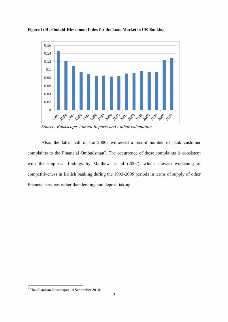
The result was a tendency towards concentration, as measured by the Herfindahl-Hirschman

Index (HHI) for total assets. As shown in Figure 1, the high HHI levels recorded during

2005-2008 suggest anti-competitive practice in the loan market in British banking during the

period3.

2 Ashton and Pham (2007) list 61 M&A activities between banks and Building Societies during 1988-2006.

3 According to the current screening guidelines of the US Department of Justice, the banking industry is

regarded as competitive if HHI is less than 1000, somewhat concentrated if HHI lies between 1000 and 1800,

and highly concentrated if HHI is larger than 1800.

3

Figure 1: Herfindahl-Hirschman Index for the Loan Market in UK Banking

Source: Bankscope, Annual Reports and Author calculation

Also, the latter half of the 2000s witnessed a record number of bank customer

complaints to the Financial Ombudsman4. The occurrence of these complaints is consistent

with the empirical findings by Matthews et al (2007), which showed worsening of

competitiveness in British banking during the 1993-2005 periods in terms of supply of other

financial services rather than lending and deposit taking.

4 The Guardian Newspaper 14 September 2010.

4

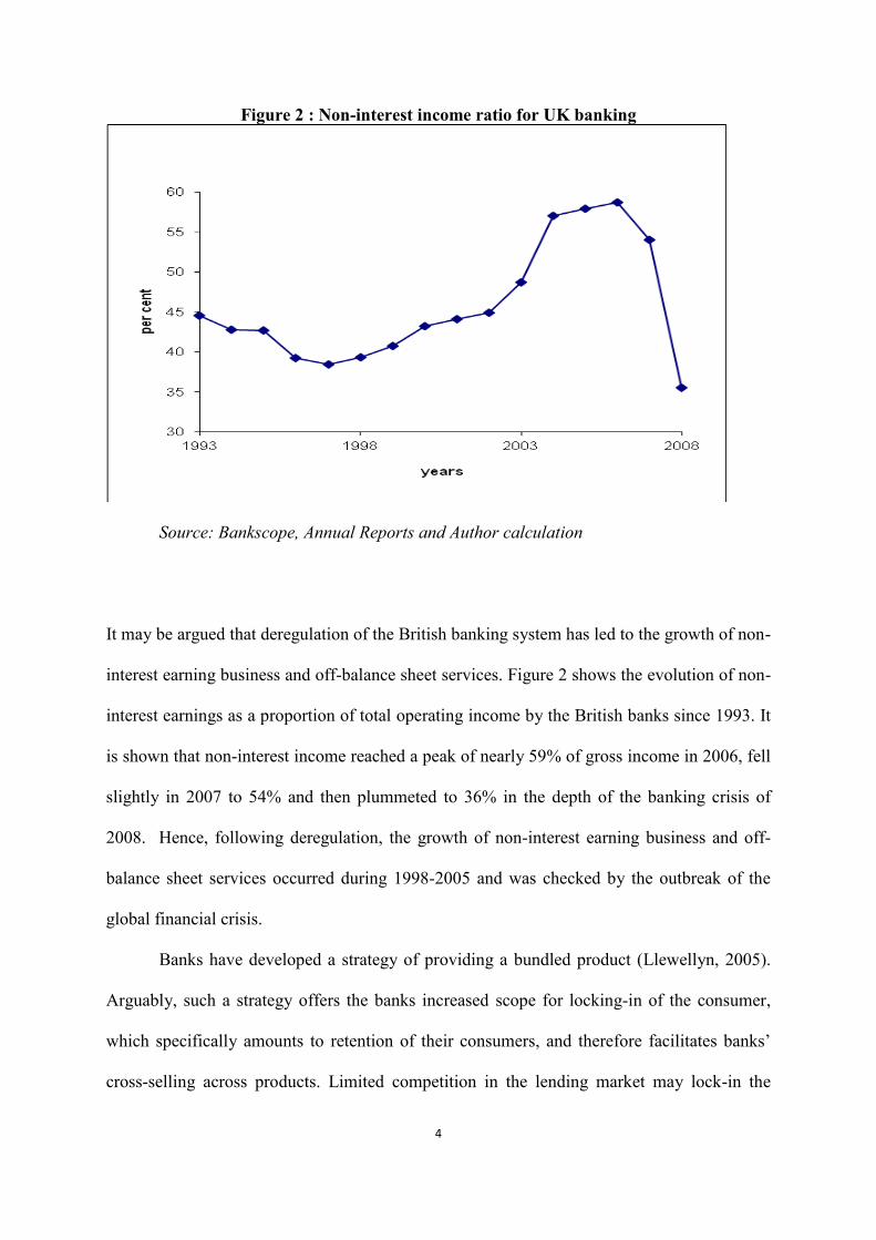
Figure 2 : Non-interest income ratio for UK banking

Source: Bankscope, Annual Reports and Author calculation

It may be argued that deregulation of the British banking system has led to the growth of non-

interest earning business and off-balance sheet services. Figure 2 shows the evolution of non-

interest earnings as a proportion of total operating income by the British banks since 1993. It

is shown that non-interest income reached a peak of nearly 59% of gross income in 2006, fell

slightly in 2007 to 54% and then plummeted to 36% in the depth of the banking crisis of

2008. Hence, following deregulation, the growth of non-interest earning business and off-

balance sheet services occurred during 1998-2005 and was checked by the outbreak of the

global financial crisis.

Banks have developed a strategy of providing a bundled product (Llewellyn, 2005).

Arguably, such a strategy offers the banks increased scope for locking-in of the consumer,

which specifically amounts to retention of their consumers, and therefore facilitates banks’

cross-selling across products. Limited competition in the lending market may lock-in the

5

bank consumers’ demand for loans as well as their demand for other financial services, where

the purchase of one bank service may be conditional on the purchase of another, which may

deter the customers from searching for the best individual product..

Previous research has found that switching costs and cross-selling have an impact on

the pricing strategy of suppliers and competitiveness in the market place (Farrell and

Klemperer, 2006). In addition to the repeat-purchase of identical good over periods in the

case of single product producers, an additional dimension that influences the pricing strategy

of the multiple product firms is contemporaneous selling of the follow-on goods (i.e. cross-

selling). The underlying implication is that the holding-up problem as the result of switching

cost has dynamic and cross-section static dimension for multiple product firms. With respect

to the former, producers compete on the lifecycle prices of the identical goods; a supplier

prices low if they recognise that their current market share would be helpful in holding on to

their existing customers in the future. The lower price in the current period can be viewed as

front-loaded compensation, where the producer uses the current price as a loss-leader. Such a

strategy can work if only the producer can effectively transform rent across periods. The

strength of the “lock-in” effect in the future determines the “market share” competition in the

present and reflects the pricing behaviour. The increase in the value of the market share that

would be locked into the future would enhance supplier’s incentive to carry out such a

strategy. With respect to the latter, producers compete on the bundle of products; multi-

product producers advertise their loss-leader core products but expect consumers who buy

their advertised products to buy other products too (Farrell and Klemperer, 2006). A supplier

reduces price of the core product than it would be if the supplier perceives the value of

transforming rent across products. Again, the likelihood of cross-selling other products to

recoup cost of the loss-leader core product would lead to the change in the producer’s

strategy. Such a strategy can work if only the producer can effectively transform rent across

6

products. Taking into account those two dimensions, switching costs and cross-selling offer a

means for suppliers to design a pricing strategy to a particular customer not just for a single

product but for a bundle of products, for multiple periods. The pricing behaviour of multiple

product firms motivated by the overall profit maximization over the long-term relationship

with their consumers has a bearing on the intrinsic inter-temporal pricing of suppliers and

also predicts the contemporaneous cross-subsidization across different products (Ausubel,

1991; Stango, 1998).

The literature on switching costs and cross-selling in banking is sparse (Li et al.,

2005). Empirical studies on cross-selling of commercial banks attempt to address the

incentives and outcomes of commercial banks to offer concurrent lending and investment-

banking services within the context of relationship banking. The general finding derived

from the literature is that banks price loans and underwriting services in a strategic way so as

to gain competitive advantage and extract value through their relationship with their

consumers (Laux and Walz, 2009; Calomiris and Pornrojnangkool 2009). With respect to

switching costs, Sharpe (1997) tests for the effects of switching costs on the pricing

behaviour of banks in the retail deposit market in the US. The research shows that the retail

deposit rate is positively related to household in-migration, which is consistent with the idea

that the faster growing market enhances the value of the current market share in the future

and incentivises banks to set interest rates that are more attractive to new consumers. A

similar result is confirmed by Hannan et al., (2003) and Hannan (2008). Shy (2002) uses an

undercut-proof equilibrium model to estimate switching cost in the market for deposits in

Finland and suggests that switching costs could be as high as 11% of the average balance of

deposit account. Kim et al. (2003) develop an empirical model which fits data to directly

estimate the magnitude and significance of the switching cost. Kim et al (2003) apply a

transition probability model of switching providers in the market for bank loans to the

7

Norwegian banking industry over the period 1988 to 19965. It is found that switching costs

are about one-third of the average interest rate on loans, which suggests creation of a

significant lock-in of bank consumers. The principal aim of this paper is to accommodate the

multiple-production characteristics of banks in the theoretical framework set up in Kim et al

(2003)6 to evaluate the development of competitiveness in British banking as a result of

cross-selling and switching costs.

III. The Theoretical Model

Kim et al. (2003) provides the theoretical framework for the presence of switching costs for

loans across time7. Consider n banks competing in a given lending market, with different

interest rates on loans. The consumers (i.e. borrowers) are assumed to have an imperfectly

elastic demand for loans8. Each consumer borrows a quantity of loans in each of the infinite

discrete periods. The borrower maximizes his utility by choosing a bank, taking into account

the interest rate on loans charged by all banks in the market. Borrowers are allowed to switch

among banks in any period. However, switching is costly; the magnitude of the switching

cost is common knowledge to banks and borrowers. The probability of switching (i.e.

transition probability9), is a function of the interest rate on loans and switching costs. The

demand for loans faced by each bank can be derived by aggregating the transition

probabilities over all borrowers even if the switching decision is not observable. The changes

in the market share of each bank across time are partly driven by borrowers’ switching.

5 Arguably, the switching cost faced by a borrower in the lending market would be non-negligible due to the

asymmetric information between borrowers and lenders. Borrowers face switching cost when they change to a

new lender since they are informationally captured by the existing lender (Sharp, 1990). Due to switching costs,

products which are homogenous ex ante become heterogeneous ex post (Klemperer, 1995). 6 A salient merit of the model in Kim et al. (2003) is that it provides a plausible theoretical underpinning for

estimation of the magnitude and significance of switching costs without requiring customer-specific data. 7 In what follows, we refer to the switching costs across periods as dynamic cross-selling while the cross-selling

from the provision of loans to OBS is referred to as static contemporaneous cross-selling. 8 The assumption is that a given bank and its rivals have the same sensitivity of the transition probability of

randomly selected borrowers to changes in the interest rate on loans. 9 The transition probabilities are assumed to be Markovian.

8

Following the derivation in Kim et al. (2003)10

, it can be shown that bank i’s market

share in the lending market at time t follows a law of motion given by11

:

11,,,1011,,

n

SPPaaSa

n

ntRiti

i

titi (1)

Where ti , denotes the market share of bank i at time t; and 1, ti refers to time t-1; S is the

magnitude of switching costs; 1a is the sensitivity of the transition probability to the bank’s

interest rate on loans. It is assumed that 01 a since the higher probability of borrowing

from bank i is associated with a lower relative interest rate charged by the bank; ia0 is the

bank-specific intercept, which captures bank heterogeneity; tiP , is the interest rate on loans

charged by the bank ; and tRiP ,, is the interest rate charged by bank i’s rivals12

.

Using a static representation of the familiar Monti-Klein model for bank i, the profit

of the bank at any point in time can be written as13

:

GSLwDGSOLCGSrOPLP DSoL ,,,, (2)

Subject to balance sheet identity: L+GS=D, where L refers to the quantity of loans, GS

denotes the quantity of government securities, and D is the quantity of loanable funds. OPo

refers to non-interest fee-based income, while O refers to the quantity of fee-based activities

(i.e. OBS). Sr is the interest rate on government securities and assumed to be bank-invariant

10

Kim et al., (2003) theoretical framework indicates that a bank has to decrease its interest rate on loans lower

enough to compensate for switching costs in order to successfully poach its rivals’ consumers. On the other

hand, once the bank has successfully poached its rivals’ consumers it can charge an interest rate on loans

slightly higher than its rivals without losing the consumers, ceteris paribus, due to switching costs. 11

The effect of switching cost on the market share of the bank at time t varies with the size of the bank. In

particular, larger than average banks would benefit from the switching costs since they have a larger consumer

base to lock in, while smaller than average banks would be worse off because more consumers are locked out. 12

As suggested by Kim et al. (2003), equation (1) remains valid where the econometricians observe only a noisy

version of the prices, such as prices which are unadjusted for output characteristics since the noises can be

absorbed by the bank-specific intercept. 13

Subscripts are omitted for simplicity.

9

and exogenously given. LP is the interest (price) rate on loans. wDGSOLC ,,,, is the non-

interest operating cost. Cost of funds ( )D and labour costs (w) are assumed to be

exogenously given in line with the standard banking model.

From the first-order conditions for profit maximization with respect to the price at any

point in time, we obtain:

L

O

O

C

O

OP

L

CP

L

PL O

DLL

i.e.

L

OMCMRMCMR OOLL

(3)

Rearranging (3) we have:

L

OMCMC

L

OMRMR OLOL

(4)

Equations (3)-(4) indicate that being a multiple-output producer, the bank would use loans as

loss-leader as long as the loss in revenue of loans can be compensated by the gain in cross-

selling off-balance sheet (OBS) services.

In a multiple-period setting, the necessary condition for the bank to maximize the

present value of its life time profit

t

ti

t

iV ,, at any point in time (denoted byτ) by

setting up the interest rate on loans at time (i.e. ),iP is 0,

,

,

,

t i

tit

i

i

PP

V. ,iP

affects not only the time profit but also the profits in the subsequent periods. The reason

for this is that the quantity of loans at any period affects the demand for loans in the period

that follows and also the demand for loans in the period that follows influences the demand

10

for OBS services contemporarily. Allowing for contemporaneous cross-selling from the

provision of loans to fee-based non-interest income, the optimal interest rate strategy can be

expressed as.14

t

t

t

t

t

tOti

ttitiL

O

O

C

O

OP

aSg

n

nPCm

1

,

11,,1

(5)

Where tiPCm , is the spread between the interest rate on loans and the marginal cost of loans

of bank i, i.e.

t

Di

i

titiL

CPPCm

,,, and is the one-period discount factor; 1, ti

is the market share of loans for bank i at time t+1, ti , refers to time t, S indicates the

magnitude of the switching cost and 1tg is the market growth rate for loans at time t+1, and

n is the number of banks in the lending market.

Equation (5) captures the relation between the price-cost margin of loans and the

current market share in the lending market, the market share in the future period and the

reimbursement from the cross-selling of OBS activities. It accommodates both dynamic and

contemporaneous cross-selling. Both types of cross-selling induce a smaller price-cost

margin of loans at time t, ceteris paribus. The first type refers to the inter-temporal supply of

loans due to switching cost (the first term). The bank believes that the current market share in

the loan market is valuable for future market share because the bank is able to lock in its

existing consumers. Hence, the bank sets a lower interest rate on loans in the current period.

Put differently, the lower interest rate on loans at time t is a loss-leader of the future market

share in the lending market. The second type of cross-selling is between loans and OBS

14

The optimal interest rate strategy given by Kim et al., (2003) only contains the first two components of

Equation (5) in the case of the presence of switching cost across periods. In our framework, the

contemporaneous cross-selling is conditional on the quantity of loans demanded at any period, the principal of

the optimal path of the interest rate on loans as elaborated in Kim et al., (2003) holds.

11

activities contemporaneously (the third term). The bank sets a lower interest rate on loans

since the bank believes that the demand for loans at time t would lead to the

contemporaneous demand for OBS services at the same time, which would bring in net

revenue associated with OBS to compensate for the loss of the revenue in the provision of

loans. The lower interest rate on loans at time t is a loss-leader of the demand for OBS

services at time t.

In the absence of both types of cross-selling, the optimization problem of the bank

reduces to the conventional case of a one-period oligopoly (i.e. the second term) in the

lending market. The oligopoly power of the bank, however, is subject to consumers’

sensitivity of the transition probability to interest rate on loans (i.e. <0).

To link the magnitude of switching cost to the degree of competition in the loan

market, we model S as a time-varying industry-specific bank-invariant switching cost

variable:

tt MCS 00 (6)

where 0C represents time-invariant psychological elements relating to inertia and tM is the

time-varying industry-specific bank-invariant degree of competition in the lending market.

The sign of 0C indicates the impact of psychological elements on the magnitude of switching

cost. The coefficient 0 indicates the impact of the change of competition on the switching

cost in the lending market; its sign a priori is indeterminate. On the one hand, the industry

organization literature tends to suggest that an increase in competition induces a decrease in

the switching cost, i.e. 00 , and hence reflects increased fragility of long-term

relationships in a more competitive environment (Petersen and Rajan, 1995). However, the

“winner’s curse” hypothesis suggests 00 due to the concern of banks to win a “lemon” in

12

a more competitive lending market15

. Moreover, banks’ endogenous effort to enhance the

capital value of relationship with borrowers in order to protect the bank-borrower tie in

competition would also induce a higher switching cost in competition (Elasa, 2005).

Equation (5) contains a component representing contemporaneous cross-selling.

Similar to the dynamic cross-selling of loans across multiple periods, the intention of banks

using loans as a loss- leader to cross-sell OBS activity contemporaneously has to be

accommodated by the demand side of OBS activities. In what follows, we use the transitional

probability of loans across periods of time, presented in Kim et al., (2003), to capture

consumers’ utility maximization.

We assume there are differences across banks in the quality of fee-based services.

Consumers value quality. Further, we assume there is an incompatibility cost borne by the

consumer at time t in the case of switching to another bank in which the consumer does not

purchase loans at the same period of time; we denote the incompatibility cost as m16

.

Thus, the probability of purchasing fee-based services in the same bank which

provides loans is:

mqqf tjtitii ,,, ,Pro (7)

tiq , is the quality indicator of bank i in providing fee-based services and tjq , is the quality

indicator of the rival bank j in providing fee-based services.

15

It is hypothesized that “bad” borrowers have more incentive to exploit the “shopping around” freedom among

banks induced by the increase in competition. This increases the difficulty by banks to distinguish between the

“good” borrowers, who switch in order to mitigate the “holding-up” problem of the existing lending

relationship, and the “bad” ones (Northcott, 2004). 16

As explained by Farrell and Klemperer (2006), such incompatibility cost is essentially an endogenous

switching cost. In order to increase the difficulty borne by their consumers to purchase the follow-on products

from other providers, producers have incentives to manipulate compatibility costs by making their follow-on

products more compatible with their core product and less compatible with their rivals’ products.

13

The probability of bank i to attract consumers who purchase loans from rival banks to

purchase OBS services from i is;

jt,R,it,it,ij mq,mqfPro (8)

jm is an (n-1) vector of incompatibility costs, in which each of the elements equal to m

except for j.

In aggregate, transitions are unobserved. Thus, the formulation of the probability of

switching to purchase fee-based services from i, even if bank i is not a supplier of loans,

unconditional on the rival’s identity, is given by:

t,KiK

t,j

jt,R,it,iijt,iiRL

Lmq,mqfPro (9)

Where tjL , is the quantity of loans of bank j at time t; tKiK

tj

L

L

,

, is the probability that a

randomly selected rival’s consumer is one who purchases loans from bank j. Therefore, the

demand for OBS activities faced by bank i at time t, induced by selling loans of the bank at

time t, is17

:

t,iiRt,R,it,iit,it,i ProLProLO (10)

tiL , is bank i’s output of loans at time t, while tRiL ,, is the rival’s (of bank i) output of loans at

time t.

17

Noticeably, the tiO , does not represent the total OBS activities provided by bank i; it is the part which is

relevant to contemporary cross-selling from loans to OBS services. Essentially, it presents a threshold that stops

the borrowers of bank i from purchasing OBS services from rival banks.

14

Using a first-order linear approximation on the transaction probabilities, we have:

mqqbPro t,R,jt,i1t,ii (11)

1n

mqqbPro t,R,jt,i1t,iiR

(12)

where tRjq ,, is the average quality of the rivals of bank i. Similar to Equation (9), Equation

(12) describes the transition probability of a randomly selected rivals’ customer. We assume

that the sensitivity of the transition probability to bank i’s quality of services equals to that of

the rivals of bank i. Substituting (10) and (11) into (9), we have:

)1

(,,

,1,,,1,,,11,

n

LLmbLLqqbO

tRi

titRittRjtti (13)

From (13), mqqbL

OtRjti

ti

ti

,,,1

,

, (14)

01 b if customers value the quality of fee-based financial services. In the case where

incompatibility cost exists, 0m . We further allow m to be time-varying and bank-invariant

and model it as a function of the degree of competition in the lending market.

tt Mmm 10 (15)

0m is assumed to be constant across our sample period, indicating the time-invariant

incompatibility cost. Such incompatibility cost includes the fixed search cost for a different

provider of financial services as well as the transaction cost dealing with multiple bank

15

relationship in providing loans and financial services. tM is the degree of competition in the

lending market. Equation (14) therefore links the time-variant incompatibility cost to the

change in the degree of competition in the lending market. Equation (15) sets up a

framework to allow us to examine the impact of the change in the degree of competition in

the loan market on cross-selling from loans to OBS services. The empirical value of 1 has

implications for the presence of the endogenous lock-in of OBS services, in response to the

change in the degree of competition in the lending market. If 01 , the bank strategically

increases the incompatibility cost in order to hold their borrowers’ consumption of OBS

services induced by the provision of loans once the lending market becomes more

competitive. Alternatively, 01 suggests that the incompatibility cost faced by consumer

(i.e. the bank’s ability to cross-sell OBS service from the bank’s perspective) is higher when

the lending market becomes less competitive. Substituting (15) into (14), gives the extent of

contemporary cross-selling undertaken by the bank:

ttRiti

ti

tiMmqqb

L

O10,,,1

,

,

Substituting Equation (15), (14) and (6) into (5) yields the first of our estimating equations:

tOttRjtitO

ti

tittOti Mbqqban

ngCmbPCm ,11,,,,1

1

,

1,10,01,1

(16)

Where t

t

t

to

tOO

C

O

OP

,

Substituting Equation (6) into Equation (1) produces the second of our estimating equations:

BMaBaCPPa ttRiti

i

ti 0110,,,10, (17)

Where 1,11

1

ti

n

n

nB .

16

IV. Data and Variables

We collect an unbalanced panel of UK bank level data for the period 1993-2008 from

Bankscope18

. Since our theoretical models of cross-selling require that sample banks operate

in the same market, we remove foreign banks and non-conventional banks from our sample.

Mergers are dealt with by aggregation of the financial statements to create a single composite

bank for the entire period. Since our theoretical model relies on the assumption that changes

in the market share of each bank across time imply switching behaviour by borrowers, we

filter the change in the market share induced by M & A. Industry level data and macro data

are obtained from Bank of England. Nominal data are deflated by the Consumer Price Index

(CPI) using 2005 as the base year. Our estimation of the change in the degree of competition

in the lending market is obtained from the H-statistic based on the Panzer and Rosse model

(1987). The sample is split into two parts of equal length (1993-2000 and 2001-2008) and

allows for the variation of H-statistics across the two sub-periods19

.

The test of the H-statistics is based on the properties of a reduced form log-linear revenue

equation for a panel data set of banks, hence:

J

j

K

k

itkitk

J

j

jitjjitj

i

it XwpostwR1 11

0 lnlnln (18)

where R represents the interest income of bank i at time t20

, the ws are J input prices for each

bank, the K X terms are exogenous bank specific variables that affect the bank’s revenue and

cost functions. The bank-specific intercept i

0 captures the heterogeneity across banks and

18

Our sample starts from 1993 excluding the 1991-1992 recession, we exclude 2009 because of the low

availability of the number of observations in Bankscope and the pollution to the data from further mergers and

the banking crisis. 19

Do we have other motivation for such split? 20

Interest income includes income on loans and other earning assets, such as government securities. The above

definition does not introduce biases into our estimation of competition in the lending market, given in the

theoretical literature which assumes that competition in market for other earning assets can be proxied by

perfect competition. Arguably, such an assumption is more realistic for advanced financial markets such as the

UK.

17

is a stochastic term. We adopt a two-input factor specification in our empirical application

(j=1,2): total loanable funds (the sum of deposits and money market funding and other

funding) and non-interest operating cost (the expenditure associated with labour and physical

capital). The price for total loanable funds is calculated as the ratio of total interest

expenditure to total loanable funds, and the price for non-interest operating cost is given by

the ratio between non-interest operating cost and total assets. We adopt the vector of bank-

specific variables, kitX , that have been used widely in the literature to estimate the H-

statistic. First, we control for the size effect on gross interest revenue by taking the natural

logarithm of total assets (LNASSET)21

. To take into account the influence of revenue

generation from the provision of OBS services on interest income, we introduce the ratio of

total operating income over total interest income (REOBS). We include the ratio of financial

capital over total earning assets to signal the constraint of capital on the supply of credit

(CAP). Finally, we consider the quality of the loan portfolio, measured by the ratio of total

loan loss reserves over total gross consumer loans (NPL). The idea is that an increase in

provisions is a diversion of capital from earnings, which could have a negative effect on

revenue. Alternatively, a higher level of provisions indicates a more risky loan portfolio and

therefore a higher level of compensating return. The variable post is a dichotomous dummy

variable, which takes the value zero for the period 1993-2000 and unity for 2001-2008. The

H-statistic is calculated from the reduced form revenue equation; it measures the sum of

elasticities of total revenue of the bank with respect to the bank’s input prices. In the context

of Equation (18),

2

1

1

j

jH is the degree of competition for 1993-2000, while

21

We are aware of the caution posed by Bikker et al., (2009) regarding the inclusion of scale variables such as

total assets in the set of control variables in the revenue equation during the estimation of H-statistics. Bikker et

al. (2009) argue that total assets proxy for the quantity of outputs. In our case, the focus is on loans, which form

only a part of total assets. The fact that we control for total assets in our equation does not imply a constant

quantity of loans, or a constant ratio of loans over total assets.

18

)(2

1

2 j

j

jH

is the degree of competition for 2001-2008. Following Olivero, et al.

(2011), among others, we interpret the magnitude of H as a measure of the degree of

competition in the loan market, with larger values of H indicating stronger competition.

An important feature of the H-statistic is that the tests must be undertaken on

observations that are in long run equilibrium. This suggests that competitive capital markets

will equalise risk-adjusted rates of return across banks such that, in equilibrium, rates of

returns should be uncorrelated with input prices. The equilibrium test is performed by

recalculating the Rosse-Panzar statistic by replacing total revenue as the dependent variable

in equation (18) with pre-tax profit to total assets (ROA) and keeping other specifications

unchanged, as shown in equation (19).

J

j

K

k

itkitk

J

j

jitjjitj

i

it uXwpostw1 1

'

1

''

0 lnlnln (19)

The long-run equilibrium tests for pre- and post- 2000 are done using 02

1

1 j

jE

and 0)(2

1

'

2 j

jjE , respectively. Since our variation of competition in the lending

market is related to two sub-periods, Equation (16) and (17) are thus restated as Equation (20)

and (21).

titOtRjtitO

ti

tittitextOex

i

tim

vpostbqqb

an

npostg

n

ngCmbMAR

,,11,,,,1

1

,

1,101,1,10,,11

(20)

tiextRiti

i

ti postBaBaCPPa ,011,,,10, (21)

19

Where t

t

titimL

CPCmMAR

,,,

, i

0 is the composite intercept term. It includes the non-

interest marginal cost of loans at the industry level and bank-specific intercept to catch the

heterogeneity22

. Notably, 0mmex and 0CCex since exm and exC include an additional

component representing the first sub-period, which is the reference category in our

examination of competition. ti , and ti , are the stochastic terms.

The dependent variable in Equation (20), timMAR ,, , is the difference between the

interest rate on loans and the interest rate on loanable funds. The interest rate on loanable

funds is calculated by the ratio of total interest expenditure to total loanable funds as we did

in Equation (18) and (19). The income statements of the banks do not always separate interest

revenue between interest earned on loans and interest earned from other earning assets. Thus,

the ratio of interest received to the sum of loans and other earning assets is a weighted

average of the average return on loans and the average return on other earning assets (RO).

Following Matthews et al., (2007), the average interest on loans is calculated by subtracting

the weighted yearly average of the 3-month interbank rate (RB) from the total interest

earnings per interest earning asset.23

If RB is a good proxy for RO, then the PL will be

measured with a non-systematic error, which will be absorbed into the general error in the

regression equation and therefore result in unbiased estimates.

Turning to the independent variables of Equation (21), we assume that tO, , the

difference between the marginal revenue and marginal cost of OBS services, is a constant

22

This is equivalent to the assumption of a linear non-interest cost function. 23

The calculated series for the full sample are available from the authors on request. Since we use the

outstanding stock of net loans which is the difference between gross loans and loan loss reserves, the implicit

interest rate on loans has been risk-adjusted.

20

coefficient across banks (i.e., a time-invariant and bank-invariant coefficient), and therefore it

merges with a constant24

.

The market growth rate at time t+1, 1tg is calculated as the sum of the quantity of

loans of our sample of banks at time t+1 divided by the same at time t and n is the number

of our sample banks at time t. The discount factor, t , is calculated using the three-month

interest rate on T-bill in line with Kim et al., (2003). The bank-specific market share at time

t+1 1, ti and is given by the quantity of loans of the bank i at time t+1 divided by the sum of

the quantity of loans of all our sample banks at time t+1. We use the ratio of total operating

income over total operating cost as the indicator of the overall quality of OBS services ( q ).

Such choice is mainly motivated by the banking literature using cost-income ratio to measure

the operational efficiency of banks. The quality of OBS services of bank i’s rival is calculated

by

ij

tjtjtRj qsq ,,,, ,

n

i

ti

tj

tj

L

Ls

1

,

,

, , is the share of each rival bank in terms of total loans

supplied by the industry as a whole. The difference in the interest rate on loans between the

bank i and its rivals in Equation (17b) (i.e. tRiti PP ,,, ) is calculated in a similar way. Table 1

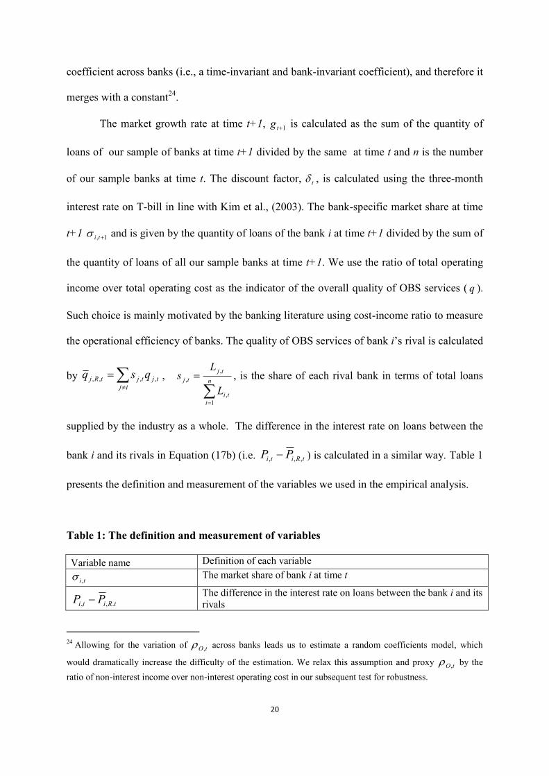
presents the definition and measurement of the variables we used in the empirical analysis.

Table 1: The definition and measurement of variables

Variable name Definition of each variable

ti , The market share of bank i at time t

tRiti PP .,, The difference in the interest rate on loans between the bank i and its

rivals

24

Allowing for the variation of tO, across banks leads us to estimate a random coefficients model, which

would dramatically increase the difficulty of the estimation. We relax this assumption and proxy tO, by the

ratio of non-interest income over non-interest operating cost in our subsequent test for robustness.

21

B 1,

11

1

ti

n

n

n

timMAR ,, The difference between the interest rate on loans and the interest rate

on loanable funds.

1,11

tittn

ng

The product of market growth rate between time t and time t+1 and

discount factor and the market share at time t+1 and 1n

n

N The number of banks at time t

t The three-month interest rate on T-bill

RB The 3-month interbank rate

tRiti qq ,,, The ratio of total operating income over total operating cost

tiO ,, The ratio of non-interest operating income over non-interest

operating cost

ln R Natural log of the interest income

lnROA Natural log of pre-tax profit to total assets

)( ,,1 tiwLn The ratio of total interest expenditure to total loanable funds

)( ,,2 tiwLn The ratio between non-interest operating cost and total assets

NPL The ratio of total loan loss reserves over total gross consumer loans

LNASSET Natural log of total assets (deflated)

REOBS The ratio of total operating income over total interest income

CAP The ratio of financial capital over total earning assets

GDPG Real GDP growth rate

POST

The bilateral dummy variable, which takes the value 0 for the

period 1993-2000 and value 1 for 2001-2008.

Table 2: Summary statistics of variables

Variable name Obs Mean Std. Dev. Min Max

ti , 1092 0.014 0.036 0.000 0.256

tRiti PP ,,, 1092 0.033 0.271 -1.872 5.665

B 1003 0.000 0.036 -0.243 0.017

timMAR ,, 1092 0.032 0.269 -2.501 5.566

1,11

tittn

ng

1003 0.084 0.209 0.000 1.381

N 1092 68.779 5.100 57.000 73.000

t 1092 4.934 1.298 1.240 7.110

RB 1092 5.463 0.996 3.670 7.340

tRjti qq ,,, 1092 0.236 1.829 -10.771 25.913

tiO ,, 1091 0.703 1.133 -16.158 27.381

ln R 1092 4.771 2.484 -0.693 10.583

lnROA 1092 0.182 0.044 0.000 1.365

)( ,,1 tiwLn 1092 -3.237 0.553 -6.723 0.693

22

)( ,,2 tiwLn 1085 -3.855 1.012 -7.784 -0.630

NPL 1092 0.027 0.050 0.000 0.457

LNASSET 1092 7.726 2.575 2.238 14.453

REOBS 1092 0.902 1.483 -0.142 24.833

CAP 1092 0.148 0.291 -0.091 6.500

GDPG 1092 0.035 0.012 -0.007 0.045

Table 2 presents the summary statistics of the variables; there are no abnormal

patterns reflected in the behaviour of the means and their dispersion.

V. Estimation and empirical results

We jointly estimate Equations (18), (19), (20) and (21) using Nonlinear-Three-Stage-Least-

Squares with one-way fixed effects using the LSDV approach25

. The endogenous variables

1, ti , ti , and the relative interest rate on loans are instrumented by lead and the lag of

market share up to three years26

, one time period lag of the relative interest rate on loans,

ti , t, and the ratio of personal expenditure over total assets of the bank i relative to its

rivals27

. As a test for robustness, we report the empirical results of four variants of the model in

Table 3. Model 1 assumes a constant O across banks and time, and imposes long-run

equilibrium in the loan market. Model 2 tests for long-run equilibrium in the loan market.

Model 3 relaxes the assumption of the constant price of OBS services in both time and bank

dimensions and use a proxy variable, the ratio of non-interest operating income over non-

interest operating cost28

. This adds a new coefficient to be estimated in equation (20), namely

( exmb1 ), and also allows us to separately identify 1b (the sensitivity of the transition

probability to the bank’s quality of OBS services) and exm (the reference incompatibility

cost). Model 4 imposes the restriction of 0exm .

25

While the majority of the banking literature using H-statistics estimates Equation (18) and (19) separately, the

Breusch-Pagan test of independence shows the presence of contemporaneous correlation of the residuals of the

two equations at 1% significant level, suggesting the need for system estimation. 26

Kim et al. (2003) also adopt the lead and lag of three years as their instruments motivated by the finding of

Degryse and van Cayseele (2000) of a 2.39 year average time length for loans. 27

Cost variables are appropriate instruments for output price in both homogeneous and differentiated markets

(Berry, 1994). It is calculated in the same manner as the relative quality indicator and relative interest rate on

loans. 28

Such treatment is equivalent to assuming the equality between marginal cost (marginal revenue) and average

cost (average revenue).

23

Table 3: Nonlinear Three-Stage Least Squares; No observations = 586; Standard

Errors in parenthesis

Variable Parameter Model 1 Model 2 Model 3 Model 4

Equation 18: Dependent Variable lnRit

)ln( ,,1 tiw 1 0.556***

(0.041

0.558***

(0.041)

0.557***

(0.041)

0.557***

(0.041)

)ln( ,,2 tiw 2 0.073***

(0.027)

0.074***

(0.027)

0.073***

(0.027)

0.073***

(0.027)

)ln(* ,,,1 tiwpost 1 -.087***

(0.019)

-.087***

(0.019)

-.087***

(0.019)

-.087**

(0.019)

)ln(* ,,2 tiwpost 2 0.071***

(0.015)

0.071***

(0.015)

0.071***

(0.015)

0.071***

(0.015)

tiNPL , 1 0.338

(0.221)

0.339

(0.221)

0.357

(0.221)

0.336

(0.221)

tiLNASSET , 2 0.924***

(0.026)

0.925***

(0.026)

0.926***

(0.026)

0.926***

(0.026)

tiREOBS , 3 -.077***

(0.011)

-.077***

(0.011)

-.077***

(0.011)

-.077***

(0.011)

tiCAP , 4 -.296

(0.249)

-.296

(0.249)

-.294

(0.248)

-.294

(0.248)

Equation 19: Dependent Variable lnROAit

)ln( ,,2,,1 titi ww *

1 0.008

(0.007)

- - -

)ln( ,,1 tiw '

1 - 0.039

(0.035)

0.038

(0.035)

0.039

(0.035)

)ln( ,,2 tiw '

2 - 0.001

(0.008)

0.000

(0.008)

0.000

(0.008)

)ln(* ,,2,,1 titi wwpost *

1 0.004

(0.005)

- - -

)ln(* ,,,1 tiwpost '

1 - -.008

(0.012)

-.008

(0.012)

-.008

(0.12)

)ln(* ,,,2 tiwpost '

2 - 0.002

(0.007)

0.002

(0.007)

0.002

(0.007)

tiNPL , '

1 0.236

(0.250)

0.248

(0.222)

0.245

(0.221)

0.245

(0.221)

tiLNASSET , '

2 0.004

(0.010)

0.008

(0.012)

0.008

(0.012)

0.008

(0.012)

tiREOBS , '

3 -.001

(0.001)

-.003

(0.002)

-.003

(0.002)

-.003

(0.002)

tiCAP , '

4 0.157

(0.114)

0.150*

(0.091)

0.153*

(0.090)

0.153*

(0.90)

Equation (20): Dependent variable: itMAR and equation (21): Dependent variable: it

ti , 1/ 1a -15.56***

(0.690)

-16.42***

(1.026)

-15.53***

(0.951)

-15.63***

(0.944)

1,11

tittn

ng exC 3.220***

(0.188)

3.359***

(0.227)

3.167***

(0.210)

3.189***

(0.212)

24

1,11

*

tittn

ngpost 0 1.188***

(0.109)

1.246***

(0.123)

1.177***

(0.116)

1.185***

(0.115)

tRjti qq ,,, Ob 1 0.014***

(0.005)

0.016**

(0.007)

- -

tiOP,

exmb1

- - -.002

(0.027)

-

Post 1 1.356*

(0.725)

1.138*

(0.633)

- -

)(* ,,,,, tRjtitiO qqP 1b

= = 0.008

(0.005)

0.008

(0.005)

post*tiOP

,

1 = = 3.107

(2.809)

3.004*

(1.841)

211 H 0.629***

(0.042)

0.631***

(0.042)

0.630***

(0.042)

0.630***

(0.042)

21212 H 0.614***

(0.037)

0.615***

(0.037)

0.614***

(0.037)

0.614***

(0.037)

21 D -.016**

(0.008)

-.016**

(0.008)

-.016**

(0.008)

-.016**

(0.008)

211 '' E - 0.039

(0.041)

0.039

(0.041)

0.039

(0.041)

21212 '''' E - 0.033

(0.036)

0.033

(0.035)

0.033

(0.035)

exm

- - -.215

(3.573)

-

Note: The number of observation is different from that in Table 2 due to our employment of instrumental

variables. The figures in the parentheses are robust-White heteroscedastic-consistent standard errors. * indicates

10% significant level, ** indicates 5% significant level and *** indicates 1% significant level. Bank-specific

fixed effects are included in the estimation.

Concentrating on the estimates for the H statistic, it can be seen that the unit price of

funds and non-interest operating cost are both positively related to interest revenue at the 1%

level, in both periods. The magnitude of the H-statistics for the first sub-period, 1993-2000, is

0.629 (H1), which is significantly different from zero at 1%. While the magnitude of the H-

statistic for the second sub-period, 2001-2008, is 0.614 (H2), again is statistically significantly

different from zero at 1%. Therefore, the competition in the UK lending market seems to be

characterised by monopolistic competition throughout 1993-2008, which is consistent with

the general finding in previous studies that have used the Rosse-Panzar approach for the

25

UK29

. The comparison between the magnitude of H1 and H2 suggests that the degree of

competition in 2001-2008 was lower than in 1993-2000.

The estimation and testing results for Equations (20) and (21) show that the point

estimate of α1, the slope of the transition probability function of bank loans, is less than zero.

Therefore, the higher interest rate charged by banks on loans would trigger the incentive of

existing borrowers to switch, as required by our theoretical model. The aggregated term of

time-invariant switching cost in the lending market and that of the period 1993-2000, exC , is

statistically significant. The significant and positive value of 0 shows a higher switching

cost in the period 2000-2008 compared with the period 1993-2000, suggesting an increase in

switching cost in a less competitive lending market. The estimated coefficient on the relative

quality indicator of financial services is statistically positive, indicating that banks with

higher relative efficiency attract more demand for OBS services, in line with the prediction of

the theoretical model30

. Finally, 1 is positive and statistically significant, suggesting that

the transition probability for the consumer to purchase OBS service from the bank that is not

its supplier of credit is lower in the period 2000-2008 compared to the period 1993-2000.

This finding suggests that contemporaneous cross-selling is more likely when the competition

in the loan market is less intensive.

Our results challenge the conventional view that the increase in competition in the

lending market leads banks to exercise a “loss-leader strategy” of reducing the interest rate on

29

For example, Molyneux et al. (1994) and Bikker and Haaf (2002) find improved competition in the 1980s and

1990s. Claessens and Laeven (2004) find relatively strong competition during the 1990s, while Casu and

Girardone (2006) find a relatively low level of competition with an H-statistic of around 0.3. The H-statistics

estimated by Matthews et al. (2007) for major British banks are in the region of 0.5-0.75. 30

The result is based on the assumption that OBS services have higher marginal revenue than marginal cost, i.e.

0,

tiO . While the current specification does not allow us to distinguish between the sensitivity of transition

probability of OBS services to the bank’s quality of financial services (i.e 1b ) and the gap between the marginal

revenue and the marginal cost of OBS services (i.e. tiO ,, ), our theoretical framework indicates that cross-

selling between loans and OBS services is economically meaningful only if there is a trade-off in revenue

between loans and OBS services (Equation (3)).

26

loans to attract consumers, and cross-sell other financial products that compensate for the loss

in interest income on loans.

Our interpretation of the above evidence is as follows. The intention by consumers to

purchase the best quality of fee-based OBS service is tempered by the increase in the

likelihood of the rejection of loans by their supplier of loans in the near future. Such a

situation is more likely to become a concern for consumers when the competition in the loan

market is low and switching costs are high. The insight that switching costs in the loan

market and the incompatibility cost of using an alternative provider of OBS services would

induce banks to charge lower interest rates on loans in a less competitive lending market

sheds doubt on the reliability of using the traditional interest rate spread to measure the

degree of competition.

We test for the robustness of the main results in three ways. First, in Model 2 we

remove the constraint of long-run equilibrium in the lending market ex ante and the test for

H-statistics, and test for the presence of long-run equilibrium condition ex post. The results

show that the equilibrium condition could not be rejected in the sub-periods and the results

were unaffected.

Second, to reflect the view that the profitability and revenue of a bank is highly

sensitive to the business cycle we add a pure time series variable, real GDP growth rate

(GDPG) to our estimation of the H-statistics (Eq (18)) and the long-run equilibrium condition

(Eq (19)) in the loan market( results not shown)31

. However, this variable was not statistically

significant in each of the model variants and again the main results were unaffected

Third, we relax the assumption of the constant O in both time and bank dimensions

and use a proxy variable, the ratio of non-interest operating income over non-interest

31

By allowing for the exogenous market growth rate in Equation (20) and (21), the pro-cyclical pattern of the

overall borrowing activity has be controlled.

27

operating cost32

. This adds a new coefficient to be estimated in equation (20), namely

( exmb1 ), and also allows us to separately identify 1b (the sensitivity of the transition

probability to the bank’s quality of OBS services) and exm (the reference incompatibility

cost). Again the results are largely unchanged

However, the sensitivity of the transitional probability of the bank consumer to the

quality of OBS services ( 1b ) and the impact of the change in competition in the lending

market on the incompatibility cost of OBS purchase ( 1 ) lose statistical significance. A

closer examination shows that the insignificant coefficient, exm , is the main reason for an

insignificant coefficient on tiO ,, ( exmb1 )33

. The coefficient exm represents the sum of time-

invariant incompatibility cost and the incompatibility cost for 1993-2000. When both

components are negligible, a zero value is a special case and is consistent with the theoretical

model. In Model 4 we impose the restriction of 0exm34

, and re-estimate the model.

The restriction of 0exm does not lead to a discernible statistical difference in the

estimates. Furthermore, 1 appears to be statistically significantly at the 10%, implying the

contemporary cross-selling situation only occurs in the less competitive lending market (i.e.

2001-2008). The coefficient 1b has the expected positive sign but it is only significant at 13%

level. However, we view this as prima facie evidence for the argument that the bank

consumer values the quality of financial services in the purchase of OBS services.

32

Such treatment is equivalent to assuming the equality between marginal cost (marginal revenue) and average

cost (average revenue). 33

This is judged from the same sign and the similar high p-value (above 0.95). 34

This is equivalent to excluding tiO ,

from independent variables in Equation (20).

28

VI. Conclusion

We have estimated and tested an empirical model of banking behaviour that encompasses

cross-selling of off-balance sheet services and switching costs in the UK during 1993-2008.

In general, the estimated parameters of the model conform to our theoretical priors. We

obtain evidence which suggests that the second half of the sample period saw an increase in

switching costs between providers of loan products. Also, we find that as a result of

weakening competition in the loan market in the second half of the sample period, bank

consumers faced higher costs of switching from their loan provider to an alternative provider.

In addition, the consumers faced higher costs of purchasing from an alternative provider of

off-balance sheet services. Contemporaneous cross-selling is therefore greater when

competition in the loan market is weaker. British banks engage more in cross-selling as a

means of holding on to their customers by bundling together off-balance sheet services and

loans when the loan market is less competitive.

Our findings challenge the conventional view that banks undertake a loss-leader

strategy of under-pricing loan products to capture bank customers and cross-sell non-interest

financial services in competition. However, our research has three shortcomings. First, the

model presented here deals with contemporaneous cross-selling and not inter-temporal cross-

selling. It is possible that banks undertake loss-leader strategies in an inter-temporal

framework as in the traditional customer-loan relationship model. Second, we assume the

price of other financial services is exogenously given, which can be challenged if the bank

possesses certain market power in the pricing of OBS. Thirdly, our research employs

aggregate bank data rather than disaggregated data relating to bank products. Nevertheless, it

is a first step to modelling cross-selling and switching costs in British banking. While

signalling the need for more theoretical and empirical work in the area of strategic behaviour

of banks, the findings of this paper have a strong policy resonance that requires further study.

29

References

Ashton, J. and Pham, K. (2007), “Efficiency and Price Effects of Horizontal Bank

Mergers”CCP Working Paper 07-09.

Ausubel, L. (1991), “The Failure of Competition in the Credit Market", American Economic

Review, 81, 50-81.

Berry, S.T., Levinsohn, J., Pakes, A., (1995). “Automobile Prices in Equilibrium”.

Econometrica, 63, 841–890.

Bikker, J.A., Haaf, K., (2002), “Competition, Concentration and Their Relationship: An

Empirical Analysis of the Banking Industry”, Journal of Banking and Finance, 26,

2191-2214.

Bikker, J.A., Shaffer, S., Spierdijk, L., (2009). “Assessing Competition with the Panzar–

Rosse Model: The Role of Scale, Costs, and Equilibrium”, In: Presented at the 22nd

Australasian Banking and Finance Conference, Sydney, Australia, December.

Calomiris, C. W., and Pornrojnangkool, T., (2009), “Relationship Banking and the Pricing of

Financial Services”, Journal of Financial Services Research, 35, 189-224.

Casu, B., and Girardone, G., (2006), “Bank Competition, Concentration, and Efficiency in

the Single European Market”, The Manchester School, 74, 441-468

Claessens, S., and Laeven, L., (2004), “What Drives Bank Competition? Some International

Evidence”, Journal of Money, Credit, and Banking, 36, 563-584.

Degryse, H., and Van Cayseele, P., (2000), “Relationship Lending within a Bank Based

System: Evidence from European Small Business Data”, Journal of Financial

Intermediation, 9, 90–109.

Elsas, R. (2005). Empirical determinants of relationship lending. Journal of Financial

Intermediation, 14, 32–57.

Farrell, J. and Klemperer, P., (2006), “Coordination and Lock-in: Competition with

Switching Costs and Network Effects”, Competition Policy Centre, Institute of

Business and Economic Research, UC Berkeley. (Available at

http://escholarchip.org/uc/item/9n26k7v1)

Kim M, Kliger D and Vale B (2003), ‘Estimating Switching Costs: the Case of Banking’,

Journal of Financial Intermediation, 12, 25-56.

Klemperer, P. (1995), “Competition when Consumers Have Switching Costs: An Overview

with Applications to Industrial Organization Macroeconomics, and International

Trade", Review of Economic Studies, 62, 515-539.

Laux, C., and Walz, U., (2009), “Cross-Selling Lending and Underwriting: Scope Economies

and Incentives”, Review of Finance, 13, 241-367.

Li S, Sun B and Wilcox R T (2005), ‘Cross-selling Sequentially Ordered Products: An

Application to Consumer Banking Services’, Journal of Marketing Research, XLII,

May, 233-239.

Llewellyn, D T., (2005), “Competition and Profitability in European Banking: Why are

British Banks so Profitable?” Economic Notes 34, 279-311.

Matthews, K., Murinde, V., Zhao, T., (2007). “Competitive Conditions among the Major

British Banks”. Journal of Banking and Finance 31, 2025–2042.

Molyneux, P., Lloyd-Williams, D., Thornton, J., (1994), “Competitive Conditions in

European Banking”, Journal of Banking Finance, 18, 445-459.

Northcott, C., (2004), “Competition in Banking: A Review of the Literature”, Working Paper

2004-2, Bank of Canada.

Panzar, J., and Rosse, J., (1987), “Testing for Monopoly Equilibrium,”. Journal of Industrial

Economics, 35, 443-456.

30

Petersen, M.A., and Rajan, R.G., (1995), “The Effect of Credit Market Competition on

Lending Relationships”, Quarterly Journal of Economics, 110, 406-443.

Sharpe, S. (1990), “Asymmetric Information, Bank Lending and Implicit Contracts: A

Stylized Model of Customer Relationships", The Journal of Finance, 45, 1069-1087.

Sharpe, S. (1997), “The Effect of Consumer Switching Costs On Prices: A Theory and Its

Application to the Bank Deposit Market", Review of Industrial Organization, 12, 79-

94.

Shy, O. (2002), ‘A Qquick-and-easy Method for Estimating Switching Costs’, International

Journal of Industrial Organization, 20, 71-87