Carbon Dioxide Fluid-Flow Modeling and Injectivity …. Department of the Interior U.S. Geological Survey Scientific Investigations Report 2011–5083 Carbon Dioxide Fluid-Flow Modeling

U.S. Department of the InteriorU.S. Geological Survey

Scientific Investigations Report 2011–5083

Carbon Dioxide Fluid-Flow Modeling and Injectivity Calculations


By Lauri Burke

Scientific Investigation Report 2011–5083

U.S. Department of the InteriorU.S. Geological Survey

U.S. Department of the InteriorKEN SALAZAR, Secretary

U.S. Geological SurveyMarcia K. McNutt, Director

U.S. Geological Survey, Reston, Virginia: 2011

For more information on the USGS—the Federal source for science about the Earth, its natural and living resources, natural hazards, and the environment, visit http://www.usgs.gov or call 1-888-ASK-USGS

For an overview of USGS information products, including maps, imagery, and publications, visit http://www.usgs.gov/pubprod

To order this and other USGS information products, visit http://store.usgs.gov

Any use of trade, product, or firm names is for descriptive purposes only and does not imply endorsement by the U.S. Government.

Although this report is in the public domain, permission must be secured from the individual copyright owners to reproduce any copyrighted materials contained within this report.

Suggested citation:Burke, Lauri, 2011, Carbon dioxide fluid-flow modeling and injectivity calculations: U.S. Geological Survey Scientific Investigations Report 2011–5083, 16 p.

http://www.usgs.gov

http://www.usgs.gov/pubprod

http://store.usgs.gov

iii

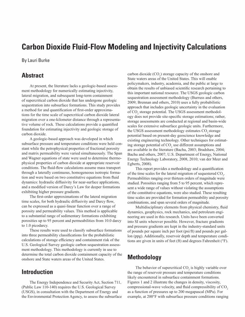
ContentsAbstract ...........................................................................................................................................................1Introduction.....................................................................................................................................................1Methodology ...................................................................................................................................................1Fluid-Flow Modeling ......................................................................................................................................2Hydraulic Diffusivity.......................................................................................................................................3Sensitivity Analysis for Hydraulic Diffusivity Flow Modeling .................................................................4Darcy’s Law of Fluid Flow .............................................................................................................................6Injectivity .........................................................................................................................................................6The Maximum Pressure Differential for Injectivity ..................................................................................7Results from Darcy’s Law of Fluid Flow ......................................................................................................9Darcy Sensitivity Analysis ..........................................................................................................................10Permeability Classifications .......................................................................................................................11Discussion and Conclusions ......................................................................................................................14Acknowledgments .......................................................................................................................................15References Cited..........................................................................................................................................15

Figures 1. Density and viscosity of pure carbon dioxide for pressures up to 200 MPa

at isothermal conditions of 200°F ...............................................................................................2 2. Compressional-wave velocity and fluid compressibility of pure carbon dioxide

as a function of pressure .............................................................................................................3 3–8. Hydraulic diffusivity time scale for lateral migration of supercritical carbon dioxide

as a function of fractional porosity and: 3. 10 darcy permeability ............................................................................................................4 4. 1.0 darcy permeability ...........................................................................................................4 5. 1.0 millidarcy permeability ...................................................................................................5 6. 1.0 microdarcy permeability ................................................................................................5 7. 1.0 nanodarcy permeability ..................................................................................................5 8. 1.0 picodarcy permeability ...................................................................................................5

9. First-order approximation for the time scale of sequestered carbon dioxide lateral movement, based on hydraulic diffusivity fluid flow, is given as a function of permeability from 10 darcy to 1.0 picodarcy and porosities from 5 to 95 percent ........6

10. Graphical representation of the maximum pressure differential, ∆P ..................................7 11. Fracture gradient as a function of depth is applicable for all continuous

depositional basins .......................................................................................................................8 12–17. Darcy’s Law time scale for lateral migration of supercritical carbon dioxide as

a function of fractional porosity and: 12. 10.0 darcy permeability .........................................................................................................9 13. 1.0 darcy permeability ...........................................................................................................9 14. 1.0 millidarcy permeability ...................................................................................................9 15. 1.0 microdarcy permeability ................................................................................................9 16. 1.0 nanodarcy permeability ................................................................................................10 17. 1.0 picodarcy permeability .................................................................................................10 18. First-order approximation for the time scale of sequestered carbon dioxide

lateral movement, based on Darcy’s Law of fluid flow, is given as a function of permeabilities ranging from 10 darcy to 1.0 picodarcy and porosities ranging from 5 to 95 percent ....................................................................................................................11

iv

Tables 1. Select fluid-flow modeling parameters and physical properties of supercritical

carbon dioxide at a reservoir temperature of 200°F and a reservoir pressure of 25.5 MPa ....................................................................................................................................3

2. First-order approximations, using hydraulic diffusivity, of the time scales of carbon dioxide lateral migration given by permeability .......................................................................7

3. Darcy flow first-order approximations of carbon dioxide lateral migration given by permeability ............................................................................................................................11

4. Time scale of sequestered carbon dioxide lateral migration as a function of matrix permeability and fractional porosity properties using the constitutive equations of hydraulic diffusivity and Darcy fluid flow ........................................................12

5. Division scheme for the three permeability classifications used in the U.S. Geological Survey assessment methodology for geologic carbon sequestration ....................................... 14

Conversion Factors

SI to Inch/PoundMultiply By To obtain

Lengthcentimeter (cm) 0.3937 inch (in.)meter (m) 3.281 foot (ft) kilometer (km) 0.6214 mile (mi)

Areasquare centimeter (cm2) 0.1550 square inch (in2)

Volumecubic meter (m3) 6.290 barrel (petroleum, 1 barrel = 42 gal)

Masskilogram (kg) 2.205 pound avoirdupois (lb)

Pressurekilopascal (kPa) 0.1450 pound per square inch (lb/in2)

Densitykilogram per cubic meter (kg/m3) 0.06242 pound per cubic foot (lb/ft3) kilogram per cubic meter (kg/m3) 0.008345 pounds per gallon (ppg)kilogram per cubic meter (kg/m3) 0.000434 pounds per square inch per foot (psi/ft)

Permeabilitysquare meter (m2) 1.01325×1012 darcydarcy 9.869233×10−13 square meter (m2)

Temperature in degrees Celsius (°C) may be converted to degrees Fahrenheit (°F) as follows:°F=(1.8×°C)+32.

Temperature in degrees Fahrenheit (°F) may be converted to degrees Celsius (°C) as follows:°C=(°F–32)/1.8.

v

Table of Symbols

A Cross-sectional areaD DepthFD Fracture gradient at depthHD Hydrostatic gradient at depthK Bulk modulusk Matrix permeabilityL Lateral distanceP PressureQ Darcy fluid-flow rateν Interstitial pore velocityVp Velocity of compressional waves in the formationα Hydraulic diffusivityβ Bulk compressibility of the formationβ Fluid compressibility∆ Gradient differential∆P Maximum pressure differential Fractional porosity Fluid viscosityµ Shear modulusτ Time scale


By Lauri Burke

carbon dioxide (CO2) storage capacity of the onshore and State waters areas of the United States. This will enable policymakers, industry, academia, and the public at large to obtain the results of unbiased scientific research pertaining to this important national resource. The USGS geologic carbon sequestration assessment methodology (Burruss and others, 2009; Brennan and others, 2010) uses a fully probabilistic approach that includes geologic uncertainty in the evaluation of CO2 storage potential. The USGS assessment methodol-ogy does not provide site-specific storage estimations; rather, storage assessments are conducted at regional and basin-wide scales for extensive subsurface geologic units. Furthermore, the USGS assessment methodology estimates CO2 storage potential based on present-day geoscience knowledge and existing engineering technology. Other techniques for estimat-ing storage potential of CO2 use different assumptions and are available in the literature (Bachu, 2003; Bradshaw, 2004; Bachu and others, 2007; U.S. Department of Energy, National Energy Technology Laboratory, 2008, 2010; van der Meer and Egberts, 2008).

This report provides a methodology and a quantification of the time scales for the lateral migration of sequestered CO2. Permeabilities ranging over thirteen orders of magnitude were studied. Porosities ranging from 5 to 95 percent, which repre-sent a wide range of values without violating the assumptions of the constitutive equations, were also studied. These resulting time scales are provided for formation permeability and porosity combinations, and span several orders of magnitude.

Multidisciplinary elements from physical chemistry, fluid dynamics, geophysics, rock mechanics, and petroleum engi-neering are used in this research. Units have been converted into SI units wherever possible. However, fracture gradients and pressure gradients are kept in the industry-standard units of pounds per square inch per foot (psi/ft) and pounds per gal-lon (ppg). Additionally, reservoir depth and temperature condi-tions are given in units of feet (ft) and degrees Fahrenheit (°F).

MethodologyThe behavior of supercritical CO2 is highly variable over

the range of reservoir pressure and temperature conditions likely encountered in subsurface containment formations. Figures 1 and 2 illustrate the changes in density, viscosity, compressional-wave velocity, and fluid compressibility of CO2 as a function of pressures up to 200 megapascal (MPa). For example, at 200°F with subsurface pressure conditions ranging

AbstractAt present, the literature lacks a geologic-based assess-

ment methodology for numerically estimating injectivity, lateral migration, and subsequent long-term containment of supercritical carbon dioxide that has undergone geologic sequestration into subsurface formations. This study provides a method for and quantification of first-order approxima-tions for the time scale of supercritical carbon dioxide lateral migration over a one-kilometer distance through a representa-tive volume of rock. These calculations provide a quantified foundation for estimating injectivity and geologic storage of carbon dioxide.

A geologic-based approach was developed in which subsurface pressure and temperature conditions were held con-stant while the petrophysical properties of fractional porosity and matrix permeability were varied simultaneously. The Span and Wagner equations of state were used to determine thermo-physical properties of carbon dioxide at appropriate reservoir conditions. The fluid-flow calculations assume mass transport through a laterally continuous, homogeneous isotropic forma-tion and were based on two constitutive equations from fluid dynamics: hydraulic diffusivity for near-surface applications, and a modified version of Darcy’s Law for deeper formations exhibiting higher pressure gradients.

The first-order approximations of the lateral migration time scales, for both hydraulic diffusivity and Darcy flow, can be expressed as a quasi-linear function over a range of porosity and permeability values. This method is applicable to a substantial range of sedimentary formations exhibiting porosities up to 95 percent and permeabilities from 10.0 darcy to 1.0 picodarcy.

These results were used to classify subsurface formations into three permeability classifications for the probabilistic calculations of storage efficiency and containment risk of the U.S. Geological Survey geologic carbon sequestration assess-ment methodology. This methodology is currently in use to determine the total carbon dioxide containment capacity of the onshore and State waters areas of the United States.

IntroductionThe Energy Independence and Security Act, Section 711,

(Public Law 110-140) requires the U.S. Geological Survey (USGS), in consultation with the Department of Energy and the Environmental Protection Agency, to assess the subsurface

2 Carbon Dioxide Fluid-Flow Modeling and Injectivity Calculations

from 0 to 200 MPa, CO2 exhibits three orders of magnitude variation in fluid density, one order of magnitude variation in viscosity, approximately one order of magnitude variation in compressional-wave velocity, and four orders of magnitude variation in fluid compressibility.

Study of the physical properties of this fluid can be restricted to the pressure and temperature conditions likely encountered in sedimentary strata. Geologic sequestration of supercritical CO2 is targeted for subsurface injection and containment at depths ranging from approximately 3,000 ft to 13,000 ft. The 3,000-ft upper depth limit represents a general approximation of the minimum pressure-depth conditions at which the injected CO2 will remain in the liquid phase (Burruss and others, 2009; Brennan and others, 2010). The lower depth of 13,000 ft is based on hydrostatic fluid displace-ment in the subsurface from surface injection at pipeline pres-sures and without additional fluid compression at the surface (Burruss and others, 2009; Brennan and others, 2010).

A sedimentary formation at a depth of 8,000 ft repre-sents the midpoint between these upper and lower depth limits. According to the industry standards defined in the Schlumberger Oilfield Glossary (Schlumberger, 2011), in general, a normally geopressured region exhibits a pressure

gradient of 0.465 psi/ft. Linear extrapolation of this gradient down to 8,000 ft yields a pressure of 3,720 psi, which cor-responds to approximately 25.5 MPa. The geoscience refer-ence Encyclopedic Dictionary of Exploration Geophysics (Sheriff, 1994) provides a generalized geothermal gradient of 30 degrees Celsius per kilometer (°C/km) or 1.65 degrees Fahrenheit per one hundred feet (°F/100 ft) for shallow crustal rocks. Assuming an average surface temperature of 68°F, a formation at a depth of 8,000 ft will exhibit, in general, a temperature of 200°F. Therefore, an isopressure of 25.5 MPa and an isotherm of 200°F were selected as the reservoir condi-tions to represent an average sedimentary formation at approx-imately 8,000-ft depth. Table 1 quantifies select physical prop-erties of supercritical CO2 under these reservoir conditions.

A geologic-based approach was developed for this analysis in which the reservoir pressure and temperature conditions were held constant while the petrophysical proper-ties of fractional porosity and matrix permeability were varied simultaneously. The fractional porosity was varied, for both the hydraulic diffusivity study and Darcy fluid flow, from 5 to 95 percent, in 5-percent increments. For completeness, this wide porosity range was studied because the sequestered fluids may react with pore fluids to enhance the porosity. In the natu-ral world, porosities approaching 65 percent have been studied in shallow carbonate core plugs recovered from boreholes of the Bahamas Drilling Project (Ehrenberg and others, 2006). However, a porosity value of 100 percent represents a continu-ous fluid-filled pore space, which would represent an unlikely injection target.

Permeability values were varied over thirteen orders of magnitude, from 10.0 darcy (D) down to 1.0 picodarcy (pD), to study the widest range of formation properties potentially encountered in sedimentary strata. Permeabilities in excess of 1.0 D have been studied in Middle East Cretaceous reservoirs (Ehrenberg and others, 2008); whereas, picodarcy strata may be encountered in clays and shales (Bol and others, 1994). Due to the thirteen orders of magnitude spread in this for-mation property, the permeabilities were divided into three permeability classifications for the USGS assessment method-ology (Burruss and others, 2009; Brennan and others, 2010) for the geologic sequestration of CO2. Formations exhibiting permeabilities greater than 1.0 D were considered Class I; for-mations exhibiting permeabilities from 1.0 D to 1.0 millidarcy (mD) were considered Class II; formations exhibiting perme-abilities below 1.0 mD were considered Class III.

Fluid-Flow ModelingThe calculations for the lateral migration and contain-

ment time scale of injected CO2 were based on two constitu-tive equations from fluid dynamics. The hydraulic diffusivity equation can be used to describe the system for near-surface conditions approaching the 3,000-ft upper depth limit, and specifically for subsurface pressures that are less than

0

200

400

600

800

1,000

1,200

0.0E+00

1.0E-04

2.0E-04

Den

sity

(kg/

m3 )

Visc

osity

(Pa·

s)

0 50 100 150 200

0 50 100 150 200Pressure

(MPa)

Pressure(MPa)

A

B

Figure 1. A, density (kg/m3) and B, viscosity (Pa·s) of pure carbon dioxide for pressures up to 200 MPa (29,000 psi) at isothermal conditions of 200°F were calculated from Span and Wagner’s modern equations of state for carbon dioxide (Span and Wagner, 1996).

Hydraulic Diffusivity 3

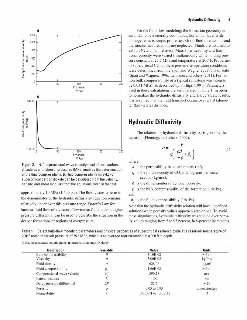
approximately 10 MPa (1,500 psi). The fluid viscosity term in the denominator of the hydraulic diffusivity equation remains relatively linear over this pressure range. Darcy’s Law for laminar fluid flow of a viscous, Newtonian fluid under a higher pressure differential can be used to describe the situation in the deeper formations or regions of overpressure.

For the fluid flow modeling, the formation geometry is assumed to be a laterally continuous, horizontal layer with homogeneous isotropic properties. Grain-fluid interactions and thermochemical reactions are neglected. Fluids are assumed to exhibit Newtonian behavior. Matrix permeability and frac-tional porosity were varied simultaneously while holding pres-sure constant at 25.5 MPa and temperature at 200°F. Properties of supercritical CO2 at these pressure-temperature conditions were determined from the Span and Wagner equations of state (Span and Wagner, 1996; Lemmon and others, 2011). Forma-tion bulk compressibility of a typical sandstone was taken to be 0.031 MPa–1 as described by Phillips (1991). Parameters used in these calculations are summarized in table 1. In order to normalize the hydraulic diffusivity and Darcy’s Law results, it is assumed that the fluid transport occurs over a 1.0 kilome-ter (km) lateral distance.

Hydraulic DiffusivityThe relation for hydraulic diffusivity, α , is given by the

equation (Flemings and others, 2002):

=

−+

⎛⎝⎜

⎞⎠⎟

k

f1

(1)

where k is the permeability in square meters (m2),

is the fluid viscosity of CO2 in kilograms per meter-second (kg/m·s),

is the dimensionless fractional porosity,

is the bulk compressibility of the formation (1/MPa),and

is the fluid compressibility (1/MPa).

Note that the hydraulic diffusivity relation will have undefined solutions when porosity values approach zero or one. To avoid these singularities, hydraulic diffusivity was studied over poros-ity values ranging from 5 to 95 percent, in 5-percent increments.

Table 1. Select fluid-flow modeling parameters and physical properties of supercritical carbon dioxide at a reservoir temperature of 200°F and a reservoir pressure of 25.5 MPa, which is an average representation of 8,000 ft in depth.

[MPa, megapascals; kg, kilograms; m, meters; s, seconds; D, darcy]

Description Variable Value UnitsBulk compressibility 3.10E-02 MPa–1

Viscosity 5.00E-05 kg/m·sFluid density 628.06 kg/m3

Fluid compressibility 1.66E-02 MPa–1

Compressional-wave velocity Vp 390.28 m/sLateral distance L 1.00 kmDarcy pressure differential ∆P 25.5 MPaPorosity 0.05 to 0.95 dimensionlessPermeability k 1.00E+01 to 1.00E-12 D

1.0E-05

8.0E-01

Flui

d co

mpr

essi

bilit

y(m

·s2 /k

g)

0

200

400

600

800

1,000

1,200

Com

pres

sion

al-w

ave

velo

city

(m/s

)

0 50 100 150 200Pressure

(MPa)

Pressure(MPa)

0 50 100 150 200

A

B

Figure 2. A, Compressional-wave velocity (m/s) of pure carbon dioxide as a function of pressures (MPa) enables the determination of the fluid compressibility. B, Fluid compressibility (m·s2/kg) of supercritical carbon dioxide can be calculated from the velocity, density, and shear modulus from the equations given in the text.


Calculating the hydraulic diffusivity of the fluid will enable the quantification of the time scale (Phillips, 1991), hd in seconds, in which a pressurized fluid pulse will propa-gate through the porous media by the relation:

hd

L=2

2 (2)

where L represents the lateral distance in meters,and

a is the hydraulic diffusivity.The fluid compressibility, , is the inverse of the

fluid bulk modulus, K, and can be determined from the compressional-wave velocity, Vp, by the relation:

V

K

p =+ 4

3

(3)

in which ρ represents the fluid density, and the shear modulus = 0 because fluids do not propagate shear stresses.

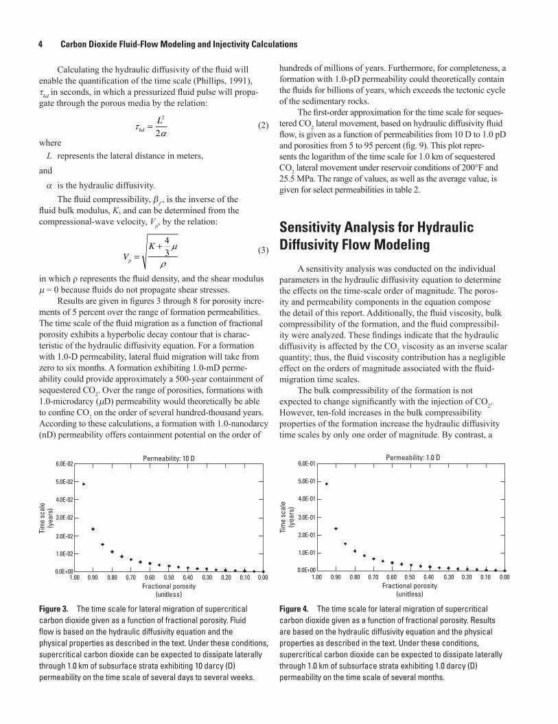
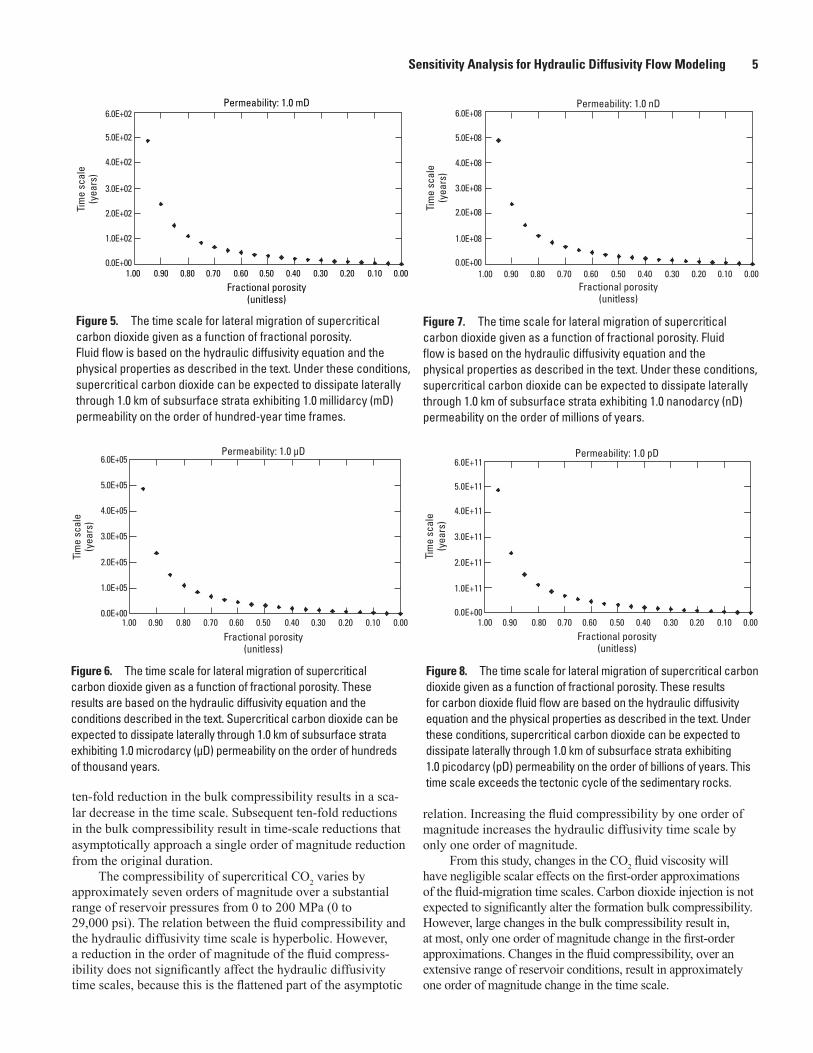
Results are given in figures 3 through 8 for porosity incre-ments of 5 percent over the range of formation permeabilities. The time scale of the fluid migration as a function of fractional porosity exhibits a hyperbolic decay contour that is charac-teristic of the hydraulic diffusivity equation. For a formation with 1.0-D permeability, lateral fluid migration will take from zero to six months. A formation exhibiting 1.0-mD perme-ability could provide approximately a 500-year containment of sequestered CO2. Over the range of porosities, formations with 1.0-microdarcy (D) permeability would theoretically be able to confine CO2 on the order of several hundred-thousand years. According to these calculations, a formation with 1.0-nanodarcy (nD) permeability offers containment potential on the order of

Figure 3. The time scale for lateral migration of supercritical carbon dioxide given as a function of fractional porosity. Fluid flow is based on the hydraulic diffusivity equation and the physical properties as described in the text. Under these conditions, supercritical carbon dioxide can be expected to dissipate laterally through 1.0 km of subsurface strata exhibiting 10 darcy (D) permeability on the time scale of several days to several weeks.

Figure 4. The time scale for lateral migration of supercritical carbon dioxide given as a function of fractional porosity. Results are based on the hydraulic diffusivity equation and the physical properties as described in the text. Under these conditions, supercritical carbon dioxide can be expected to dissipate laterally through 1.0 km of subsurface strata exhibiting 1.0 darcy (D) permeability on the time scale of several months.

Tim

e sc

ale

(yea

rs)

0.0E+00

1.0E-02

2.0E-02

3.0E-02

4.0E-02

5.0E-02

6.0E-02

Fractional porosity(unitless)

0.000.100.200.300.400.500.600.700.800.901.00

Permeability: 10 D

0.0E+00

1.0E-01

2.0E-01

3.0E-01

4.0E-01

5.0E-01

6.0E-01

Tim

e sc

ale

(yea

rs)

Permeability: 1.0 D

0.000.100.200.300.400.500.600.700.800.901.00Fractional porosity

(unitless)

hundreds of millions of years. Furthermore, for completeness, a formation with 1.0-pD permeability could theoretically contain the fluids for billions of years, which exceeds the tectonic cycle of the sedimentary rocks.

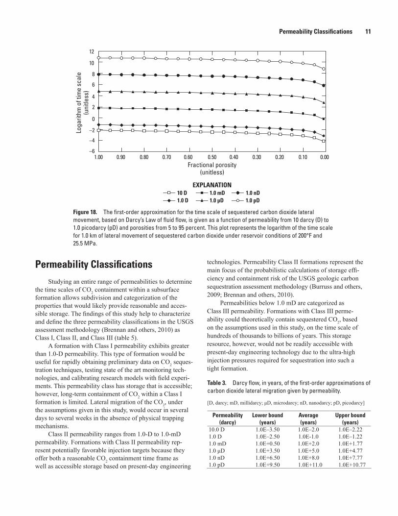
The first-order approximation for the time scale for seques-tered CO2 lateral movement, based on hydraulic diffusivity fluid flow, is given as a function of permeabilities from 10 D to 1.0 pD and porosities from 5 to 95 percent (fig. 9). This plot repre-sents the logarithm of the time scale for 1.0 km of sequestered CO2 lateral movement under reservoir conditions of 200°F and 25.5 MPa. The range of values, as well as the average value, is given for select permeabilities in table 2.

Sensitivity Analysis for Hydraulic Diffusivity Flow Modeling

A sensitivity analysis was conducted on the individual parameters in the hydraulic diffusivity equation to determine the effects on the time-scale order of magnitude. The poros-ity and permeability components in the equation compose the detail of this report. Additionally, the fluid viscosity, bulk compressibility of the formation, and the fluid compressibil-ity were analyzed. These findings indicate that the hydraulic diffusivity is affected by the CO2 viscosity as an inverse scalar quantity; thus, the fluid viscosity contribution has a negligible effect on the orders of magnitude associated with the fluid-migration time scales.

The bulk compressibility of the formation is not expected to change significantly with the injection of CO2. However, ten-fold increases in the bulk compressibility properties of the formation increase the hydraulic diffusivity time scales by only one order of magnitude. By contrast, a

Sensitivity Analysis for Hydraulic Diffusivity Flow Modeling 5

Figure 5. The time scale for lateral migration of supercritical carbon dioxide given as a function of fractional porosity. Fluid flow is based on the hydraulic diffusivity equation and the physical properties as described in the text. Under these conditions, supercritical carbon dioxide can be expected to dissipate laterally through 1.0 km of subsurface strata exhibiting 1.0 millidarcy (mD) permeability on the order of hundred-year time frames.

Figure 6. The time scale for lateral migration of supercritical carbon dioxide given as a function of fractional porosity. These results are based on the hydraulic diffusivity equation and the conditions described in the text. Supercritical carbon dioxide can be expected to dissipate laterally through 1.0 km of subsurface strata exhibiting 1.0 microdarcy (μD) permeability on the order of hundreds of thousand years.

Figure 7. The time scale for lateral migration of supercritical carbon dioxide given as a function of fractional porosity. Fluid flow is based on the hydraulic diffusivity equation and the physical properties as described in the text. Under these conditions, supercritical carbon dioxide can be expected to dissipate laterally through 1.0 km of subsurface strata exhibiting 1.0 nanodarcy (nD) permeability on the order of millions of years.

0.0E+00

1.0E+02

2.0E+02

3.0E+02

4.0E+02

5.0E+02

6.0E+02

Tim

e sc

ale

(yea

rs)

Permeability: 1.0 mD

0.000.100.200.300.400.500.600.700.800.901.00


0.0E+00

1.0E+05

2.0E+05

3.0E+05

4.0E+05

5.0E+05

6.0E+05

Tim

e sc

ale

(yea

rs)

Permeability: 1.0 µD

0.000.100.200.300.400.500.600.700.800.901.00


0.0E+00

1.0E+08

2.0E+08

3.0E+08

4.0E+08

5.0E+08

6.0E+08

Tim

e sc

ale

(yea

rs)

Permeability: 1.0 nD


(unitless)

Figure 8. The time scale for lateral migration of supercritical carbon dioxide given as a function of fractional porosity. These results for carbon dioxide fluid flow are based on the hydraulic diffusivity equation and the physical properties as described in the text. Under these conditions, supercritical carbon dioxide can be expected to dissipate laterally through 1.0 km of subsurface strata exhibiting 1.0 picodarcy (pD) permeability on the order of billions of years. This time scale exceeds the tectonic cycle of the sedimentary rocks.

0.0E+00

1.0E+11

2.0E+11

3.0E+11

4.0E+11

5.0E+11

6.0E+11

Tim

e sc

ale

(yea

rs)

Permeability: 1.0 pD


(unitless)

ten-fold reduction in the bulk compressibility results in a sca-lar decrease in the time scale. Subsequent ten-fold reductions in the bulk compressibility result in time-scale reductions that asymptotically approach a single order of magnitude reduction from the original duration.

The compressibility of supercritical CO2 varies by approximately seven orders of magnitude over a substantial range of reservoir pressures from 0 to 200 MPa (0 to 29,000 psi). The relation between the fluid compressibility and the hydraulic diffusivity time scale is hyperbolic. However, a reduction in the order of magnitude of the fluid compress-ibility does not significantly affect the hydraulic diffusivity time scales, because this is the flattened part of the asymptotic

relation. Increasing the fluid compressibility by one order of magnitude increases the hydraulic diffusivity time scale by only one order of magnitude.

From this study, changes in the CO2 fluid viscosity will have negligible scalar effects on the first-order approximations of the fluid-migration time scales. Carbon dioxide injection is not expected to significantly alter the formation bulk compressibility. However, large changes in the bulk compressibility result in, at most, only one order of magnitude change in the first-order approximations. Changes in the fluid compressibility, over an extensive range of reservoir conditions, result in approximately one order of magnitude change in the time scale.


The variability of the time scales were studied over the depth range and compared to the 8,000-ft base case. For the 3,000-ft upper depth limit, the formation temperature decreased to 118°F and the formation pressure decreased to 9.6 MPa (1,400 psi). The CO2 properties of density, compressional-wave velocity, and fluid viscosity also decrease by a scalar factor at these shallower reservoir conditions. The scalar value of the lateral migration time scale is decreased by approximately half. However, there is no change to the order of magnitude of the lateral migration time scale at 3,000-ft depth. At the 13,000-ft lower depth limit, the formation tem-perature is increased to 282°F and the formation pressure is increased to 41.5 MPa (6,000 psi). The physical properties of CO2 increase by a scalar factor at these greater depths. A neg-ligible increase occurs to the scalar value of the time scales, and there is no change to the order of magnitude of the lateral migration time scales at 13,000-ft depth.

Darcy’s Law of Fluid FlowDarcy’s Law of viscous fluid flow through a porous

media is a proportional relation between the pressure gradient over a distance, ΔP/L; fluid viscosity, ; matrix permeability, k; and cross-sectional area, A, through which the fluid passes. The fluid flow rate, Q, is defined as:

QkA P

L=

Δ (4)

Figure 9. The first-order approximation for the time scale of sequestered carbon dioxide lateral movement, based on hydraulic diffusivity fluid flow, is given as a function of permeability from 10 darcy (D) to 1.0 picodarcy (pD) and porosities from 5 to 95 percent. This plot represents the logarithm of the time scale for 1.0 km of lateral movement of sequestered carbon dioxide under reservoir conditions of 200°F and 25.5 MPa.

Darcy’s Law assumes that the fluid flow is laminar. Under hydrostatic conditions, no fluid flow occurs; in the presence of a pressure gradient, fluid flows from high pressure toward low pressure.

The interstitial pore velocity (m/s) is given by the Darcy flux divided by porosity:

vk P

L= Δ

(5)

The time frame D, in units of seconds, for Darcy flow of a viscous fluid through a porous media across a lateral distance L is expressed as:

D

L

k P=

2

Δ (6)

To obtain time-scale results that are comparable with the hydraulic diffusivity flow, the distance for the lateral migra-tion of sequestered CO2 in the Darcy fluid-flow calculations is 1.0 km.

InjectivityThe Schlumberger Oilfield Glossary (Schlumberger,

2011) defines an injectivity test as a procedure that is used to determine “the rate and pressure at which fluids can be pumped into the treatment target without fracturing the formation.” According to the reservoir engineering literature

–6

–4

–2

0

2

4

6

8

10

12

14

Loga

rithm

of t

ime

scal

e(u

nitle

ss)


(unitless)

10 D1.0 D

1.0 mD1.0 µD

1.0 nD1.0 pD

EXPLANATION

The Maximum Pressure Differential for Injectivity 7

Figure 10. Graphical representation of the maximum pressure differential, ∆P. The magnitude of the maximum pressure differential is the pressure increase, due to carbon dioxide injection, that a formation could theoretically handle before fractures are induced. For reservoir conditions at 8,000-ft depth, as detailed in the text, the maximum pressure differential ∆P is 3,698 psi, 17.8 ppg, or 25.5 MPa in engineering, oil field, and geophysical units, respectively.

Table 2. First-order approximations, using hydraulic diffusivity, of the time scales of carbon dioxide lateral migration given by permeability.

[D, darcy; mD, millidarcy; μD, microdarcy; nD, nanodarcy; pD, picodarcy]

Permeability (darcy)

Lower bound (years)

Average (years)

Upper bound (years)

10.0 D 1.0E–3.70 1.0E–2.0 1.0E–1.631.0 D 1.0E–2.70 1.0E–1.0 1.0E–0.311.0 mD 1.0E+0.30 1.0E+2.0 1.0E+2.681.0 μD 1.0E+3.30 1.0E+5.0 1.0E+5.681.0 nD 1.0E+6.30 1.0E+8.0 1.0E+8.681.0 pD 1.0E+9.30 1.0E+11.0 1.0E+11.68

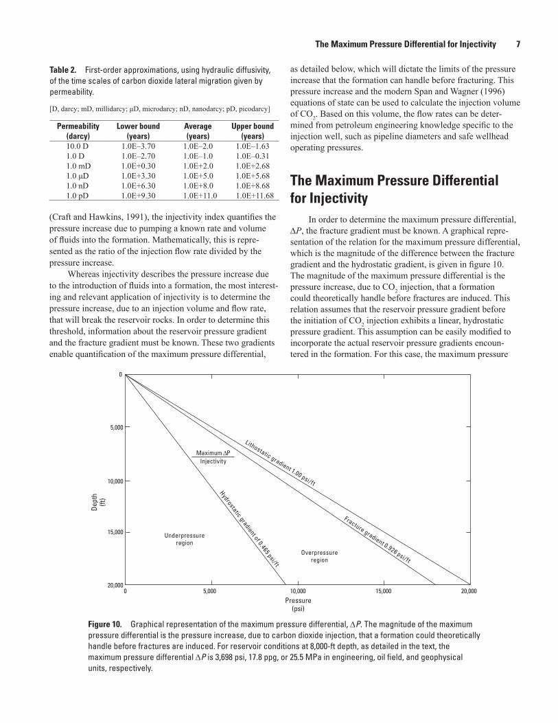
(Craft and Hawkins, 1991), the injectivity index quantifies the pressure increase due to pumping a known rate and volume of fluids into the formation. Mathematically, this is repre-sented as the ratio of the injection flow rate divided by the pressure increase.

Whereas injectivity describes the pressure increase due to the introduction of fluids into a formation, the most interest-ing and relevant application of injectivity is to determine the pressure increase, due to an injection volume and flow rate, that will break the reservoir rocks. In order to determine this threshold, information about the reservoir pressure gradient and the fracture gradient must be known. These two gradients enable quantification of the maximum pressure differential,

as detailed below, which will dictate the limits of the pressure increase that the formation can handle before fracturing. This pressure increase and the modern Span and Wagner (1996) equations of state can be used to calculate the injection volume of CO2. Based on this volume, the flow rates can be deter-mined from petroleum engineering knowledge specific to the injection well, such as pipeline diameters and safe wellhead operating pressures.

The Maximum Pressure Differential for Injectivity

In order to determine the maximum pressure differential, ∆P, the fracture gradient must be known. A graphical repre-sentation of the relation for the maximum pressure differential, which is the magnitude of the difference between the fracture gradient and the hydrostatic gradient, is given in figure 10. The magnitude of the maximum pressure differential is the pressure increase, due to CO2 injection, that a formation could theoretically handle before fractures are induced. This relation assumes that the reservoir pressure gradient before the initiation of CO2 injection exhibits a linear, hydrostatic pressure gradient. This assumption can be easily modified to incorporate the actual reservoir pressure gradients encoun-tered in the formation. For this case, the maximum pressure

Lithostatic gradient 1.00 psi/ft

Fracture gradient 0.926 psi/ftOverpressure

region

Underpressureregion

Maximum ∆PInjectivity

Hydrostatic gradient of 0.465 psi/ft

Dept

h(ft

)

Pressure(psi)

0

5,000

10,000

15,000

20,0000 5,000 10,000 15,000 20,000


differential, ∆P, would simply represent the difference between the fracture pressure gradient and the actual reservoir pressure gradient. Although these trends may not necessarily be linear in nature, this mathematical relation for calculating the maximum pressure differential is still valid. The maximum pressure differential, ∆P, evaluated at a specific depth, D, can be expressed as:

ΔP F HD D D= − (7)

where FD is the fracture gradient at the specified depthand HD is the original reservoir pressure gradient or hydrostatic

gradient evaluated at the specified depth.This relation assumes that the formation is not already fractured due to overpressuring and that ∆P will always be a positive value.

Many empirical methods exist for calculating the fracture gradient of a formation, given detailed information about the pore pressure, matrix stress coefficient, vertical matrix stresses, overburden stress, water depths, Poisson’s ratio, leak-off pressure tests, and pressure integrity tests (Hubbert and

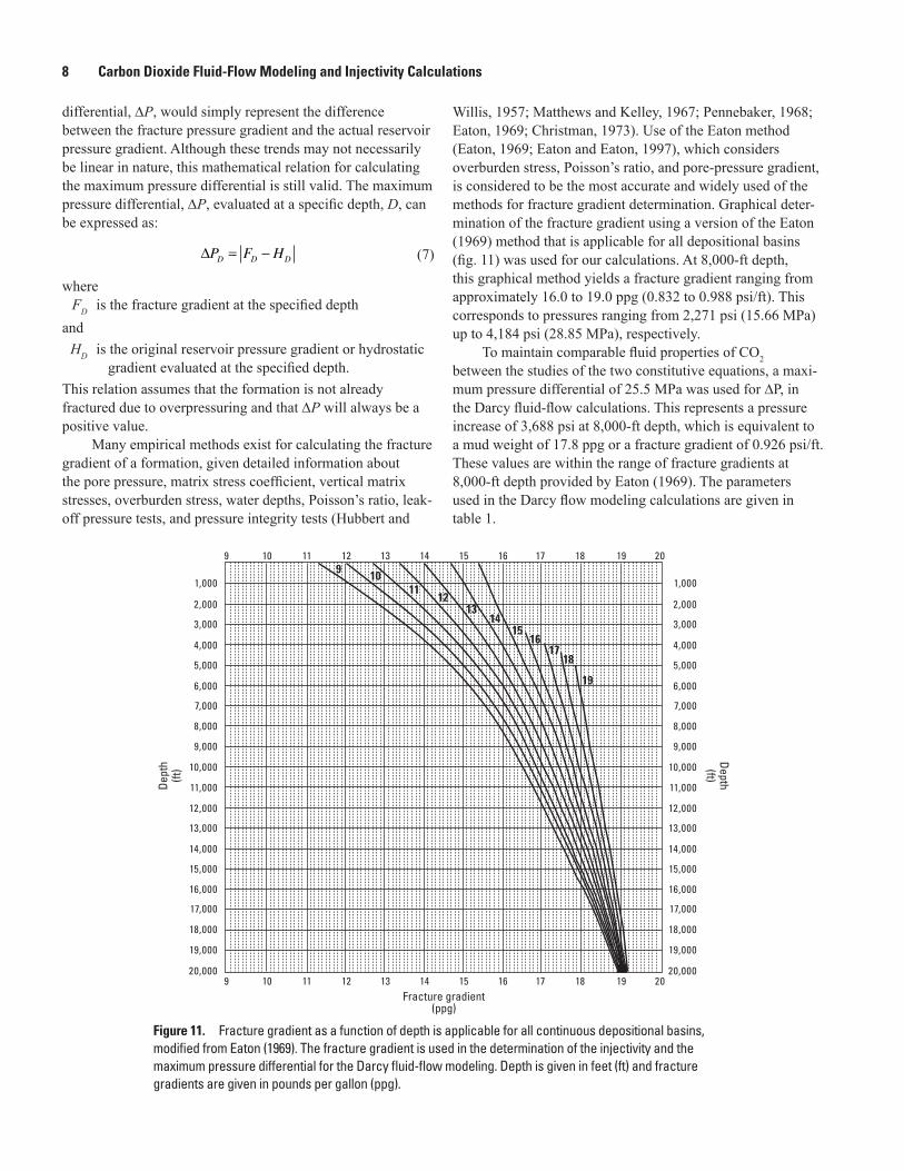
Figure 11. Fracture gradient as a function of depth is applicable for all continuous depositional basins, modified from Eaton (1969). The fracture gradient is used in the determination of the injectivity and the maximum pressure differential for the Darcy fluid-flow modeling. Depth is given in feet (ft) and fracture gradients are given in pounds per gallon (ppg).

Willis, 1957; Matthews and Kelley, 1967; Pennebaker, 1968; Eaton, 1969; Christman, 1973). Use of the Eaton method (Eaton, 1969; Eaton and Eaton, 1997), which considers overburden stress, Poisson’s ratio, and pore-pressure gradient, is considered to be the most accurate and widely used of the methods for fracture gradient determination. Graphical deter-mination of the fracture gradient using a version of the Eaton (1969) method that is applicable for all depositional basins (fig. 11) was used for our calculations. At 8,000-ft depth, this graphical method yields a fracture gradient ranging from approximately 16.0 to 19.0 ppg (0.832 to 0.988 psi/ft). This corresponds to pressures ranging from 2,271 psi (15.66 MPa) up to 4,184 psi (28.85 MPa), respectively.

To maintain comparable fluid properties of CO2 between the studies of the two constitutive equations, a maxi-mum pressure differential of 25.5 MPa was used for ∆P, in the Darcy fluid-flow calculations. This represents a pressure increase of 3,688 psi at 8,000-ft depth, which is equivalent to a mud weight of 17.8 ppg or a fracture gradient of 0.926 psi/ft. These values are within the range of fracture gradients at 8,000-ft depth provided by Eaton (1969). The parameters used in the Darcy flow modeling calculations are given in table 1.

9 1011

1213

1415

1617

18

19

1,000

2,000

3,000

4,000

5,000

6,000

7,000

8,000

9,000

10,000

11,000

12,000

13,000

14,000

15,000

16,000

17,000

18,000

19,000

20,000

1,000

2,000

3,000

4,000

5,000

6,000

7,000

8,000

9,000

10,000

11,000

12,000

13,000

14,000

15,000

16,000

17,000

18,000

19,000

20,000

Depth(ft)

Dept

h(ft

)

9 10 11 12 13 14 15 16 17 18 19 20

9 10 11 12 13 14 15 16 17 18 19 20

Fracture gradient(ppg)

Results from Darcy’s Law of Fluid Flow 9

Figure 12. The time scale for lateral migration of supercritical carbon dioxide is given as a function of fractional porosity. Fluid flow is based on Darcy’s Law and the physical properties as described in the text. Under these conditions, supercritical carbon dioxide can be expected to dissipate laterally through 1.0 km of subsurface strata exhibiting 10.0 darcy (D) permeability on the time scale of several days.

Figure 13. The time scale for lateral migration of supercritical carbon dioxide is given as a function of fractional porosity. These results are based on Darcy’s Law and the physical properties as described in the text. Under these conditions, supercritical carbon dioxide can be expected to dissipate laterally through 1.0 km of subsurface strata exhibiting 1.0 darcy (D) permeability on the time scale of several days to several weeks.

Figure 14. The time scale for lateral migration of supercritical carbon dioxide is given as a function of fractional porosity. Fluid flow is based on Darcy’s Law and the physical properties as described in the text. Under these conditions, supercritical carbon dioxide can be expected to dissipate laterally through 1.0 km of subsurface strata exhibiting 1.0 millidarcy (mD) permeability on the time scale of several decades.

Figure 15. The time scale for lateral migration of supercritical carbon dioxide is given as a function of fractional porosity. These results for carbon dioxide fluid flow are based on Darcy’s Law and the physical properties as described in the text. Under these conditions, supercritical carbon dioxide can be expected to dissipate laterally through 1.0 km of subsurface strata exhibiting 1.0 microdarcy (μD) permeability on the time scale of several tens of thousands of years.

Results from Darcy’s Law of Fluid Flow

The results for the Darcy fluid-flow modeling over the thirteen orders of magnitude variations in permeability exhibit a decreasing linear trend with increasing porosity (figs. 12–17). Note that the Darcy fluid-flow results, in general, yield a one order of magnitude difference from the hydraulic diffusivity results. This may be due to the effects of the Darcy pressure dif-ferentials enhancing the rate of lateral migration.

According to these results, CO2 may migrate laterally through a formation with 10.0-D permeability on the order of a few days. Lateral migration of CO2 through a formation

exhibiting 1.0-D permeability will occur on the time scale of months. Formations exhibiting 1.0-mD permeability have approximately six months to a 60-year confinement of the CO2 within a 1.0-km section of formation. A formation exhibiting 1.0-μD permeability would theoretically be able to confine CO2 on the order of several hundreds to tens of thousands of years. Formations with 1.0-nD permeability offer CO2 contain-ment potential in the millions to tens of millions of years. For completeness, these calculations indicate that a formation with 1.0-pD permeability yields lateral migration on the order of billions of years, which exceeds the tectonic cycle of the sedimentary basins.

0.0E+00

1.0E-03

2.0E-03

3.0E-03

4.0E-03

5.0E-03

6.0E-03

7.0E-03

Tim

e sc

ale

(yea

rs)

Permeability: 10 D

0.100.200.300.400.500.600.700.800.901.00Fractional porosity

(unitless)

0.00

0.0E+00

1.0E-02

2.0E-02

3.0E-02

4.0E-02

5.0E-02

6.0E-02

7.0E-02

Tim

e sc

ale

(yea

rs)


(unitless)

Permeability: 1.0 D

1.0E-01

1.0E+01

2.0E+01

3.0E+01

4.0E+01

5.0E+01

6.0E+01

7.0E+01

Tim

e sc

ale

(yea

rs)

Permeability: 1.0 mD

0.000.100.200.300.400.500.600.700.800.901.00


1.0E-01

1.0E+04

2.0E+04

3.0E+04

4.0E+04

5.0E+04

6.0E+04

7.0E+04

Tim

e sc

ale

(yea

rs)

Permeability: 1.0 µD


(unitless)


Figure 17. The time scale for lateral migration of supercritical carbon dioxide is given as a function of fractional porosity. Fluid flow is based on Darcy’s Law and the physical properties as described in the text. Under these conditions, supercritical carbon dioxide can be expected to dissipate laterally through 1.0 km of subsurface strata exhibiting 1.0 picodarcy (pD) permeability on the time scale of several billion years. This exceeds the tectonic cycle of the rocks and represents the extreme lower bound of this study.

1.0E-01

1.0E+10

2.0E+10

3.0E+10

4.0E+10

5.0E+10

6.0E+10

7.0E+10

Tim

e sc

ale

(yea

rs)

Permeability: 1.0 pD


(unitless)

Figure 16. The time scale for lateral migration of supercritical carbon dioxide is given as a function of fractional porosity. These fluid-flow results are based on Darcy’s Law and the physical properties as described in the text. Under these conditions, supercritical carbon dioxide can be expected to dissipate laterally through 1.0 km of subsurface strata exhibiting 1.0 nanodarcy (nD) permeability on the time scale of several million years.

1.0E-01

1.0E+07

2.0E+07

3.0E+07

4.0E+07

5.0E+07

6.0E+07

7.0E+07

Tim

e sc

ale

(yea

rs)

Permeability: 1.0 nD


(unitless)

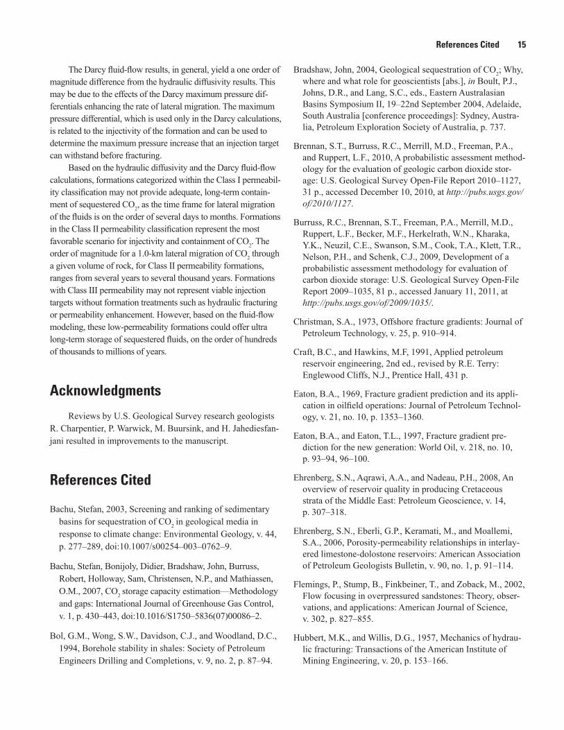
The first-order approximations for the lateral migration of CO2 exhibiting Darcy fluid flow are provided graphically in figure 18 and numerically in table 3 for the range of perme-ability values and porosity combinations. These data repre-sent the logarithm of the time scales for lateral migration, or containment potential, of CO2 through 1.0 km of formation at reservoir pressure and temperature of 25.5 MPa (3,400 psi) and 200°F, respectively. This range of values, as well as the average value, is given for select permeabilities in table 3.

The numerical values of the lateral migration time scales for all permeability and porosity combinations, are given in table 4. Note the similarities and differences in the time-scale values between the two constitutive equations. The similarities suggest that these first-order approximations, derived from two separate equations with different input values, yield a reliable estimation of the lateral migration time scale. The differences, however, indicate that scientific judgment is required to deter-mine whether the fluid properties or the pressure differential is expected to have the greater impact on the behavior in a specific injection formation. The hydraulic diffusivity equation can describe the system for pressures below approximately 10 MPa (1,500 psi) in that the fluid viscosity term exhibits quasi-linear behavior in this pressure region. Darcy fluid flow takes into account the maximum pressure differential and pressure-induced fracturing of the injection formation, which are necessary considerations in overpressured regions.

Darcy Sensitivity AnalysisThe variables of distance, fluid viscosity, and pressure

differential were studied for their contribution to the migra-tion time scales derived from the Darcy fluid-flow equation. One order of magnitude changes in the fluid viscosity result in one order of magnitude changes in the migration time scales. Increasing the fluid viscosity allows the fluid to flow at a faster rate, thereby decreasing the time scale. Increasing the pres-sure differential by one order of magnitude results in a one order of magnitude decrease in the time scale, inasmuch as the pressure increase enhances the fluid migration from higher to lower pressure regimes. Increasing the migration distance by one order of magnitude increases the time scale by one order of magnitude. Due to the proportionality of this equa-tion, order of magnitude changes in the variables are inversely proportional to the resulting order of magnitude changes in the migration time scales.

The time-scale variability over the depth range was studied and compared to the 8,000-ft base case. At the upper depth limit of 3,000 ft, the formation temperature is decreased to 118°F and the formation pressure is decreased to 9.6 MPa (1,400 psi). The CO2 properties of density, compressional-wave velocity, and fluid viscosity also decrease by a scalar fac-tor at these shallower reservoir conditions. The scalar value of the lateral migration time scale is decreased by approximately half. However, there is no change to the order of magnitude of the lateral migration time scale. At the 13,000-ft lower depth limit, the formation temperature is increased to 282°F and the formation pressure is increased 41.5 MPa (6,000 psi). The physical properties of CO2 increase by a scalar factor at these deeper depths. The scalar value of the lateral migration time scales is increased by one, and there is no change to the order of magnitude of the lateral migration time scales.

Permeability Classifications 11

Figure 18. The first-order approximation for the time scale of sequestered carbon dioxide lateral movement, based on Darcy’s Law of fluid flow, is given as a function of permeability from 10 darcy (D) to 1.0 picodarcy (pD) and porosities from 5 to 95 percent. This plot represents the logarithm of the time scale for 1.0 km of lateral movement of sequestered carbon dioxide under reservoir conditions of 200°F and 25.5 MPa.

Table 3. Darcy flow, in years, of the first-order approximations of carbon dioxide lateral migration given by permeability.

[D, darcy; mD, millidarcy; μD, microdarcy; nD, nanodarcy; pD, picodarcy]


Lower bound (years)

Average (years)

Upper bound (years)

10.0 D 1.0E–3.50 1.0E–2.0 1.0E–2.221.0 D 1.0E–2.50 1.0E-1.0 1.0E–1.221.0 mD 1.0E+0.50 1.0E+2.0 1.0E+1.771.0 μD 1.0E+3.50 1.0E+5.0 1.0E+4.771.0 nD 1.0E+6.50 1.0E+8.0 1.0E+7.771.0 pD 1.0E+9.50 1.0E+11.0 1.0E+10.77

–6

–4

–2

0

2

4

6

8

10

12

Loga

rithm

of t

ime

scal

e(u

nitle

ss)


(unitless)

10 D1.0 D

1.0 mD1.0 µD

1.0 nD1.0 pD

EXPLANATION

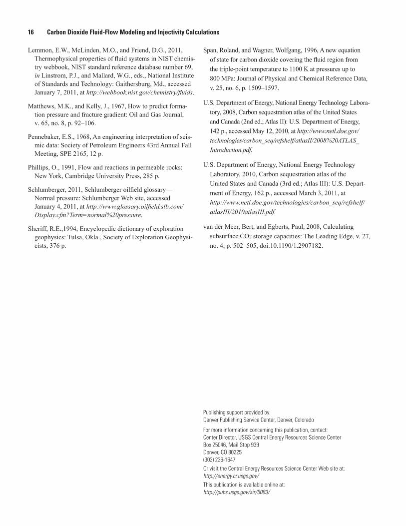
Permeability ClassificationsStudying an entire range of permeabilities to determine

the time scales of CO2 containment within a subsurface formation allows subdivision and categorization of the properties that would likely provide reasonable and acces-sible storage. The findings of this study help to characterize and define the three permeability classifications in the USGS assessment methodology (Brennan and others, 2010) as Class I, Class II, and Class III (table 5).

A formation with Class I permeability exhibits greater than 1.0-D permeability. This type of formation would be useful for rapidly obtaining preliminary data on CO2 seques-tration techniques, testing state of the art monitoring tech-nologies, and calibrating research models with field experi-ments. This permeability class has storage that is accessible; however, long-term containment of CO2 within a Class I formation is limited. Lateral migration of the CO2, under the assumptions given in this study, would occur in several days to several weeks in the absence of physical trapping mechanisms.

Class II permeability ranges from 1.0-D to 1.0-mD permeability. Formations with Class II permeability rep-resent potentially favorable injection targets because they offer both a reasonable CO2 containment time frame as well as accessible storage based on present-day engineering

technologies. Permeability Class II formations represent the main focus of the probabilistic calculations of storage effi-ciency and containment risk of the USGS geologic carbon sequestration assessment methodology (Burruss and others, 2009; Brennan and others, 2010).

Permeabilities below 1.0 mD are categorized as Class III permeability. Formations with Class III perme-ability could theoretically contain sequestered CO2, based on the assumptions used in this study, on the time scale of hundreds of thousands to billions of years. This storage resource, however, would not be readily accessible with present-day engineering technology due to the ultra-high injection pressures required for sequestration into such a tight formation.



Porosity (unitless)

Hydraulic diffusivity time scale

(years)

Darcy’s Law

time scale (years)

1.00E+01 D 0.95 1.98E-04 3.15E-040.90 4.11E-04 6.30E-040.85 6.40E-04 9.46E-040.80 8.91E-04 1.26E-030.75 1.17E-03 1.58E-030.70 1.47E-03 1.89E-030.65 1.81E-03 2.21E-030.60 2.20E-03 2.52E-030.55 2.64E-03 2.84E-030.50 3.16E-03 3.15E-030.45 3.78E-03 3.47E-030.40 4.54E-03 3.78E-030.35 5.50E-03 4.10E-030.30 6.75E-03 4.41E-030.25 8.48E-03 4.73E-030.20 1.10E-02 5.04E-030.15 1.53E-02 5.36E-030.10 2.36E-02 5.67E-030.05 4.86E-02 5.99E-03

1.00E+00 D 0.95 1.98E-03 3.15E-030.90 4.11E-03 6.30E-030.85 6.40E-03 9.46E-030.80 8.91E-03 1.26E-020.75 1.17E-02 1.58E-020.70 1.47E-02 1.89E-020.65 1.81E-02 2.21E-020.60 2.20E-02 2.52E-020.55 2.64E-02 2.84E-020.50 3.16E-02 3.15E-020.45 3.78E-02 3.47E-020.40 4.54E-02 3.78E-020.35 5.50E-02 4.10E-020.30 6.75E-02 4.41E-020.25 8.48E-02 4.73E-020.20 1.10E-01 5.04E-020.15 1.53E-01 5.36E-020.10 2.36E-01 5.67E-020.05 4.86E-01 5.99E-02

1.00E-01 D 0.95 1.981E-02 3.15E-020.90 4.107E-02 6.30E-020.85 6.405E-02 9.46E-020.80 8.906E-02 1.26E-010.75 1.165E-01 1.58E-010.70 1.469E-01 1.89E-010.65 1.810E-01 2.21E-010.60 2.197E-01 2.52E-010.55 2.641E-01 2.84E-010.50 3.161E-01 3.15E-010.45 3.782E-01 3.47E-010.40 4.541E-01 3.78E-010.35 5.498E-01 4.10E-010.30 6.751E-01 4.41E-010.25 8.479E-01 4.73E-01

Table 4. Time scale of sequestered carbon dioxide lateral migration as a function of matrix permeability and fractional porosity properties using the constitutive equations of hydraulic diffusivity and Darcy fluid flow.

[D, darcy]


Porosity (unitless)


(years)

Darcy’s Law

time scale (years)

1.00E-01 D—Continued 0.20 1.104E+00 5.04E-010.15 1.526E+00 5.36E-010.10 2.363E+00 5.67E-010.05 4.862E+00 5.99E-01

1.00E-02 D 0.95 1.981E-01 3.15E-010.90 4.107E-01 6.30E-010.85 6.405E-01 9.46E-010.80 8.906E-01 1.26E+000.75 1.165E+00 1.58E+000.70 1.469E+00 1.89E+000.65 1.810E+00 2.21E+000.60 2.197E+00 2.52E+000.55 2.641E+00 2.84E+000.50 3.161E+00 3.15E+000.45 3.782E+00 3.47E+000.40 4.541E+00 3.78E+000.35 5.498E+00 4.10E+000.30 6.751E+00 4.41E+000.25 8.479E+00 4.73E+000.20 1.104E+01 5.04E+000.15 1.526E+01 5.36E+000.10 2.363E+01 5.67E+000.05 4.862E+01 5.99E+00

1.00E-03 D 0.95 1.98E+00 3.15E+000.90 4.11E+00 6.30E+000.85 6.40E+00 9.46E+000.80 8.91E+00 1.26E+010.75 1.17E+01 1.58E+010.70 1.47E+01 1.89E+010.65 1.81E+01 2.21E+010.60 2.20E+01 2.52E+010.55 2.64E+01 2.84E+010.50 3.16E+01 3.15E+010.45 3.78E+01 3.47E+010.40 4.54E+01 3.78E+010.35 5.50E+01 4.10E+010.30 6.75E+01 4.41E+010.25 8.48E+01 4.73E+010.20 1.10E+02 5.04E+010.15 1.53E+02 5.36E+010.10 2.36E+02 5.67E+010.05 4.86E+02 5.99E+01

1.00E-04 D 0.95 1.981E+01 3.15E+010.90 4.107E+01 6.30E+010.85 6.405E+01 9.46E+010.80 8.906E+01 1.26E+020.75 1.165E+02 1.58E+020.70 1.469E+02 1.89E+020.65 1.810E+02 2.21E+020.60 2.197E+02 2.52E+020.55 2.641E+02 2.84E+020.50 3.161E+02 3.15E+020.45 3.782E+02 3.47E+02

Permeability Classifications 13

Table 4. Time scale of sequestered carbon dioxide lateral migration as a function of matrix permeability and fractional porosity properties using the constitutive equations of hydraulic diffusivity and Darcy fluid flow.—Continued

[D, darcy]


Porosity (unitless)


(years)

Darcy’s Law

time scale (years)

1.00E-04 D—Continued 0.40 4.541E+02 3.78E+020.35 5.498E+02 4.10E+020.30 6.751E+02 4.41E+020.25 8.479E+02 4.73E+020.20 1.104E+03 5.04E+020.15 1.526E+03 5.36E+020.10 2.363E+03 5.67E+020.05 4.862E+03 5.99E+02



1.00E-07 D 0.95 1.981E+04 3.15E+040.90 4.107E+04 6.30E+040.85 6.405E+04 9.46E+040.80 8.906E+04 1.26E+050.75 1.165E+05 1.58E+050.70 1.469E+05 1.89E+050.65 1.810E+05 2.21E+05


Porosity (unitless)


(years)

Darcy’s Law

time scale (years)

1.00E-07 D—Continued 0.60 2.197E+05 2.52E+050.55 2.641E+05 2.84E+050.50 3.161E+05 3.15E+050.45 3.782E+05 3.47E+050.40 4.541E+05 3.78E+050.35 5.498E+05 4.10E+050.30 6.751E+05 4.41E+050.25 8.479E+05 4.73E+050.20 1.104E+06 5.04E+050.15 1.526E+06 5.36E+050.10 2.363E+06 5.67E+050.05 4.862E+06 5.99E+05



1.00E-10 D 0.95 1.981E+07 3.15E+070.90 4.107E+07 6.30E+070.85 6.405E+07 9.46E+07



Porosity (unitless)


(years)

Darcy’s Law

time scale (years)

1.00E-10 D—Continued 0.80 8.906E+07 1.26E+080.75 1.165E+08 1.58E+080.70 1.469E+08 1.89E+080.65 1.810E+08 2.21E+080.60 2.197E+08 2.52E+080.55 2.641E+08 2.84E+080.50 3.161E+08 3.15E+080.45 3.782E+08 3.47E+080.40 4.541E+08 3.78E+080.35 5.498E+08 4.10E+080.30 6.751E+08 4.41E+080.25 8.479E+08 4.73E+080.20 1.104E+09 5.04E+080.15 1.526E+09 5.36E+080.10 2.363E+09 5.67E+080.05 4.862E+09 5.99E+08

1.00E-11 D 0.95 1.981E+08 3.15E+080.90 4.107E+08 6.30E+080.85 6.405E+08 9.46E+080.80 8.906E+08 1.26E+090.75 1.165E+09 1.58E+090.70 1.469E+09 1.89E+090.65 1.810E+09 2.21E+090.60 2.197E+09 2.52E+090.55 2.641E+09 2.84E+090.50 3.161E+09 3.15E+090.45 3.782E+09 3.47E+09

Table 5. Division scheme for the three permeability classifications used in the U.S. Geological Survey assessment methodology for geologic carbon sequestration (Brennan and others, 2010). Note that 1.0 darcy is equal to approximately 9.869233×10−13 m2.

[D, darcy; m, meter]

ClassificationPermeability range

(darcy)Permeability range

(m2)Class I Class I ≥ 1.0 D Class I ≥ 9.8692E-13DClass II 1.0 D ≥ Class II ≥ 1.0 mD 9.8692E-13 ≥ Class II ≥ 9.8692E-16Class III Class III ≤ 1.0 mD Class III ≤ 9.8692E-16

Discussion and Conclusions

Quantification of the first-order approximations of the time scales involved in the lateral migration of sequestered CO2 through a given volume of rock enables a general estimation of the containment time frames of the sequestered gas. This study investigated these time scales for formations exhibiting permea-bilities from 10.0 D to 1.0 pD and porosities from 5 to 95 percent.

The time scale of the fluid migration as a function of fractional porosity exhibits a hyperbolic decay contour that is characteristic of the hydraulic diffusivity equation. The time scale


Porosity (unitless)


(years)

Darcy’s Law

time scale (years)

1.00E-11 D—Continued 0.40 4.541E+09 3.78E+090.35 5.498E+09 4.10E+090.30 6.751E+09 4.41E+090.25 8.479E+09 4.73E+090.20 1.104E+10 5.04E+090.15 1.526E+10 5.36E+090.10 2.363E+10 5.67E+090.05 4.862E+10 5.99E+09


of fluid migration using the Darcy fluid-flow equation, however, yields a decreasing linear trend. In both cases, the order of mag-nitude, as calculated from the logarithm of the time scales, can be approximated as a quasi-linear trend over a range of permeability-porosity values. Furthermore, the similarities in the time-scale values between the two constitutive equations suggest that these first-order approximations, derived from two separate equations with different input values, yield a reliable estimation of the lat-eral migration. Therefore, the methods given in this study would be applicable to determine the general time scales of a subsurface formation, given the availability of specific information about average permeability and porosity characteristics.

Table 4. Time scale of sequestered carbon dioxide lateral migration as a function of matrix permeability and fractional porosity properties using the constitutive equations of hydraulic diffusivity and Darcy fluid flow.—Continued

[D, darcy]

References Cited 15

The Darcy fluid-flow results, in general, yield a one order of magnitude difference from the hydraulic diffusivity results. This may be due to the effects of the Darcy maximum pressure dif-ferentials enhancing the rate of lateral migration. The maximum pressure differential, which is used only in the Darcy calculations, is related to the injectivity of the formation and can be used to determine the maximum pressure increase that an injection target can withstand before fracturing.

Based on the hydraulic diffusivity and the Darcy fluid-flow calculations, formations categorized within the Class I permeabil-ity classification may not provide adequate, long-term contain-ment of sequestered CO2, as the time frame for lateral migration of the fluids is on the order of several days to months. Formations in the Class II permeability classification represent the most favorable scenario for injectivity and containment of CO2. The order of magnitude for a 1.0-km lateral migration of CO2 through a given volume of rock, for Class II permeability formations, ranges from several years to several thousand years. Formations with Class III permeability may not represent viable injection targets without formation treatments such as hydraulic fracturing or permeability enhancement. However, based on the fluid-flow modeling, these low-permeability formations could offer ultra long-term storage of sequestered fluids, on the order of hundreds of thousands to millions of years.

Acknowledgments

Reviews by U.S. Geological Survey research geologists R. Charpentier, P. Warwick, M. Buursink, and H. Jahediesfan-jani resulted in improvements to the manuscript.

References Cited

Bachu, Stefan, 2003, Screening and ranking of sedimentary basins for sequestration of CO2 in geological media in response to climate change: Environmental Geology, v. 44, p. 277–289, doi:10.1007/s00254–003–0762–9.

Bachu, Stefan, Bonijoly, Didier, Bradshaw, John, Burruss, Robert, Holloway, Sam, Christensen, N.P., and Mathiassen, O.M., 2007, CO2 storage capacity estimation—Methodology and gaps: International Journal of Greenhouse Gas Control, v. 1, p. 430–443, doi:10.1016/S1750–5836(07)00086–2.

Bol, G.M., Wong, S.W., Davidson, C.J., and Woodland, D.C., 1994, Borehole stability in shales: Society of Petroleum Engineers Drilling and Completions, v. 9, no. 2, p. 87–94.

Bradshaw, John, 2004, Geological sequestration of CO2; Why, where and what role for geoscientists [abs.], in Boult, P.J., Johns, D.R., and Lang, S.C., eds., Eastern Australasian Basins Symposium II, 19–22nd September 2004, Adelaide, South Australia [conference proceedings]: Sydney, Austra-lia, Petroleum Exploration Society of Australia, p. 737.

Brennan, S.T., Burruss, R.C., Merrill, M.D., Freeman, P.A., and Ruppert, L.F., 2010, A probabilistic assessment method-ology for the evaluation of geologic carbon dioxide stor-age: U.S. Geological Survey Open-File Report 2010–1127, 31 p., accessed December 10, 2010, at http://pubs.usgs.gov/of/2010/1127.

Burruss, R.C., Brennan, S.T., Freeman, P.A., Merrill, M.D., Ruppert, L.F., Becker, M.F., Herkelrath, W.N., Kharaka, Y.K., Neuzil, C.E., Swanson, S.M., Cook, T.A., Klett, T.R., Nelson, P.H., and Schenk, C.J., 2009, Development of a probabilistic assessment methodology for evaluation of carbon dioxide storage: U.S. Geological Survey Open-File Report 2009–1035, 81 p., accessed January 11, 2011, at http://pubs.usgs.gov/of/2009/1035/.

Christman, S.A., 1973, Offshore fracture gradients: Journal of Petroleum Technology, v. 25, p. 910–914.

Craft, B.C., and Hawkins, M.F, 1991, Applied petroleum reservoir engineering, 2nd ed., revised by R.E. Terry: Englewood Cliffs, N.J., Prentice Hall, 431 p.

Eaton, B.A., 1969, Fracture gradient prediction and its appli-cation in oilfield operations: Journal of Petroleum Technol-ogy, v. 21, no. 10, p. 1353–1360.

Eaton, B.A., and Eaton, T.L., 1997, Fracture gradient pre-diction for the new generation: World Oil, v. 218, no. 10, p. 93–94, 96–100.

Ehrenberg, S.N., Aqrawi, A.A., and Nadeau, P.H., 2008, An overview of reservoir quality in producing Cretaceous strata of the Middle East: Petroleum Geoscience, v. 14, p. 307–318.

Ehrenberg, S.N., Eberli, G.P., Keramati, M., and Moallemi, S.A., 2006, Porosity-permeability relationships in interlay-ered limestone-dolostone reservoirs: American Association of Petroleum Geologists Bulletin, v. 90, no. 1, p. 91–114.

Flemings, P., Stump, B., Finkbeiner, T., and Zoback, M., 2002, Flow focusing in overpressured sandstones: Theory, obser-vations, and applications: American Journal of Science, v. 302, p. 827–855.

Hubbert, M.K., and Willis, D.G., 1957, Mechanics of hydrau-lic fracturing: Transactions of the American Institute of Mining Engineering, v. 20, p. 153–166.

http://pubs.usgs.gov/of/2010/1127

http://pubs.usgs.gov/of/2010/1127

http://pubs.usgs.gov/of/2009/1035/


Lemmon, E.W., McLinden, M.O., and Friend, D.G., 2011, Thermophysical properties of fluid systems in NIST chemis-try webbook, NIST standard reference database number 69, in Linstrom, P.J., and Mallard, W.G., eds., National Institute of Standards and Technology: Gaithersburg, Md., accessed January 7, 2011, at http://webbook.nist.gov/chemistry/fluids.

Matthews, M.K., and Kelly, J., 1967, How to predict forma-tion pressure and fracture gradient: Oil and Gas Journal,v. 65, no. 8, p. 92–106.

Pennebaker, E.S., 1968, An engineering interpretation of seis-mic data: Society of Petroleum Engineers 43rd Annual Fall Meeting, SPE 2165, 12 p.

Phillips, O., 1991, Flow and reactions in permeable rocks: New York, Cambridge University Press, 285 p.

Schlumberger, 2011, Schlumberger oilfield glossary— Normal pressure: Schlumberger Web site, accessed January 4, 2011, at http://www.glossary.oilfield.slb.com/Display.cfm?Term=normal%20pressure.

Sheriff, R.E.,1994, Encyclopedic dictionary of exploration geophysics: Tulsa, Okla., Society of Exploration Geophysi-cists, 376 p.

Span, Roland, and Wagner, Wolfgang, 1996, A new equation of state for carbon dioxide covering the fluid region from the triple-point temperature to 1100 K at pressures up to 800 MPa: Journal of Physical and Chemical Reference Data, v. 25, no. 6, p. 1509–1597.

U.S. Department of Energy, National Energy Technology Labora-tory, 2008, Carbon sequestration atlas of the United States and Canada (2nd ed.; Atlas II): U.S. Department of Energy, 142 p., accessed May 12, 2010, at http://www.netl.doe.gov/ technologies/carbon_seq/refshelf/atlasII/2008%20ATLAS_Introduction.pdf.

U.S. Department of Energy, National Energy Technology Laboratory, 2010, Carbon sequestration atlas of the United States and Canada (3rd ed.; Atlas III): U.S. Depart-ment of Energy, 162 p., accessed March 3, 2011, at http://www.netl.doe.gov/technologies/carbon_seq/refshelf/atlasIII/2010atlasIII.pdf.

van der Meer, Bert, and Egberts, Paul, 2008, Calculating subsurface CO2 storage capacities: The Leading Edge, v. 27, no. 4, p. 502–505, doi:10.1190/1.2907182.

Publishing support provided by: Denver Publishing Service Center, Denver, Colorado

For more information concerning this publication, contact: Center Director, USGS Central Energy Resources Science Center Box 25046, Mail Stop 939 Denver, CO 80225 (303) 236-1647Or visit the Central Energy Resources Science Center Web site at: http://energy.cr.usgs.gov/This publication is available online at: http://pubs.usgs.gov/sir/5083/

http://www.glossary.oilfield.slb.com/Display.cfm?Term=normal%20pressure

http://www.glossary.oilfield.slb.com/Display.cfm?Term=normal%20pressure

http://webbook.nist.gov/chemistry/fluids

http://www.netl.doe.gov/technologies/carbon_seq/refshelf/atlasII/2008%20ATLAS_Introduction.pdf

http://www.netl.doe.gov/technologies/carbon_seq/refshelf/atlasIII/2010atlasIII.pdf

http://energy.cr.usgs.gov/

http://pubs.usgs.gov/sir/5083/

Burke—Carbon D

ioxide Fluid-Flow M

odeling and Injectivity Calculations—Scientific Investigations Report 2011–5083

Documents

Carbon Dioxide Fluid-Flow Modeling and Injectivity …. Department of the Interior U.S. Geological Survey Scientific Investigations Report 2011–5083 Carbon Dioxide Fluid-Flow Modeling