University of North DakotaUND Scholarly Commons

Theses and Dissertations Theses, Dissertations, and Senior Projects

2009

Carbon Dioxide Flooding Induced GeochemicalChanges in a Saline Carbonate AquiferAlyssa BoockUniversity of North Dakota

Follow this and additional works at: https://commons.und.edu/theses

Part of the Geology Commons

This Thesis is brought to you for free and open access by the Theses, Dissertations, and Senior Projects at UND Scholarly Commons. It has beenaccepted for inclusion in Theses and Dissertations by an authorized administrator of UND Scholarly Commons. For more information, please contactzeineb.yousif@library.und.edu.

Recommended CitationBoock, Alyssa, "Carbon Dioxide Flooding Induced Geochemical Changes in a Saline Carbonate Aquifer" (2009). Theses andDissertations. 33.https://commons.und.edu/theses/33

CARBON DIOXIDE FLOODING INDUCED GEOCHEMICAL CHANGES IN A

SALINE CARBONATE AQUIFER

by

Alyssa Boock

Bachelor of Science in Geology, University of Wisconsin-River Falls, 2002

A Thesis

Submitted to the Graduate Faculty

of the

University of North Dakota

in partial fulfillment of the requirements

for the degree of

Master of Science

Grand Forks, North Dakota

December

2009

ii

This thesis, submitted by Alyssa Boock in partial fulfillment of the requirements

for the Degree of Master of Science from the University of North Dakota, has been read

by the Faculty Advisory Committee under whom the work has been done and is hereby

approved.

_____________________________________

Chairperson

_____________________________________

_____________________________________

This thesis meets the standards for appearance, conforms to the style and format

requirements of the Graduate School of the University of North Dakota, and is hereby

approved.

_______________________________

Dean of the Graduate School

_______________________________

Date

iii

PERMISSION

Title Carbon Dioxide Flooding Induced Geochemical Changes in a Saline

Carbonate Aquifer

Department Geology

Degree Master of Science

In presenting this thesis in partial fulfillment of the requirements for a graduate

degree from the University of North Dakota, I agree that the library of this University

shall make it freely available for inspection. I further agree that permission for extensive

copying for scholarly purposes may be granted by the professor who supervised my

thesis work or, in his absence, by the chairperson of the department or the dean of the

Graduate School. It is understood that any copying or publication or other use of this

thesis or part thereof for financial gain shall not be allowed without my written

permission. It is also understood that due recognition shall be given to me and to the

University of North Dakota in any scholarly use which may be made of any material in

my thesis.

Signature ____________________________

Date _____________________________

iv

TABLE OF CONTENTS

LIST OF FIGURES……………………………………………………………………… v

LIST OF TABLES……………………………………………………………………….. vi

ACKNOWLEDGMENTS………………………………………………………………. vii

ABSTRACT……………………………………………………………………………..viii

CHAPTER

I. INTRODUCTION…………………………………………………………1

II. BACKGROUND…………………………………………………………..5

III. MATERIALS AND METHODS………………………………………... 16

IV. RESULTS……………………………………………………………….. 23

V. DISCUSSION…………………………………………………………… 37

VI. CONCLUSIONS…………………………………………………………47

APPENDICES……………………………………………………………………………50

REFERENCES…………………………………………………………………………. 83

v

LIST OF FIGURES

Figure Page

1. Stratigraphic column of the Williston Basin in North Dakota ………………….. 11

2. Oil fields in North Dakota……………………………………………………….. 15

3. Multipurpose core flooding system………………………………………………17

4. Effluent pH during flooding……………………………………………………...25

5. Effluent conductance during flooding…………………………………………....26

6. Sodium concentrations for all water flood samples……………………………... 29

7. Calcium concentrations for all water flood samples ………………………...….. 30

8. Ferrous iron concentrations for all water flood samples………………………… 31

9. Chloride concentrations for all water flood samples …..…………….…………. 32

10. Alkalinity concentrations for all water flood samples…………………………... 34

11. TDS concentrations for all water flood samples and …………………………… 35

12. Limestone cores pre- and post-CO2 flooding…………………………………….46

vi

LIST OF TABLES

Table Page

1. Stock solution preparation ……………………………………………………... 20

2. Flooding induced changes in porosity and density of rock cores……………….. 24

3. Results from chemical analysis………………………………………………….. 28

4. Density of water flood solutions………………………………………………… 36

5. DI rinse of pump B after saline water injection…………………………………. 61

6. Properties of rock cores pre- and post-flooding and geomechanical testing……. 64

7. Sample IDs and corresponding sample descriptions……………………………. 65

8. Dilution factors………………………………………………………………….. 66

9. Quality Control…………………………………………………………………...67

10. Values for pH versus volume injected graph …………………………………… 68

11. Values for conducatance versus volume injected graph………………………… 73

12. Water density calculations………………………………………………………. 78

vii

ACKNOWLEDGMENTS

I would like to extend my sincerest thanks and appreciation to my committee

chairman Dr. Zheng-Wen (Zane) Zeng for his guidance, support, and willingness to work

with me as an off-campus student. I would also like to thank my other committee

members, Dr. Scott Korom and Dr. Richard LeFever, for their help, suggestions, and

guidance with this project.

This research was generously funded by the US Department of Energy through

contracts DE-FC26-05NT42592 and DE-FC26-08NT0005643 and by North Dakota

Industry Commission (NDIC) together with Encore Acquisition Company, Hess Corporation,

Marathon Oil Company, St. Mary Land & Exploration Company, and Whiting Petroleum

Corporation under contract NDIC-G015-031.

I would like to thank Xue Jun (John) Zhou and Hong Liu for their assistance with

the operation of the core-flooding system and rock core preparation. Hanying Xu,

director of UND’s Environmental Analytical Research Laboratory, provided instruction

and guidance with the laboratory instruments. Dr. Robert Baker has provided guidance

and encouragement since I was a child, and helped push me into geology and eventually

graduate school. I would also like to thank my past and present employers for allowing

me to schedule my work around my schooling when needed.

Finally I would like to thank my family and friends for their support and

encouragement through my coursework at UND and my return to finish. A special

thanks goes to Tanya Justham for her support and friendship during my return.

viii

ABSTRACT

Carbon dioxide (CO2) has been injected into depleted oil reservoirs for enhanced

oil recovery for several decades. Injection of CO2 into geologic formations in the

Williston Basin is currently under consideration for long-term CO2 storage to reduce

anthropogenic CO2 emissions to the atmosphere. The Madison Group in the North

Dakota Williston Basin provides the greatest potential for geologic sequestration in either

deep saline aquifers or depleted oil reservoirs. Little is known about the geochemical

reactions that take place when supercritical carbon dioxide is injected into deep saline

aquifers at geologic conditions similar to those found in potential sequestration units of

the Madison Group.

Previous studies have shown the injection of carbon dioxide into a saline aquifer

makes the formation water slightly acidic, which reacts with the host rock to dissolve

carbonate minerals. Dissolution of carbonate minerals may compromise the integrity of

the formation, leading to the eventual escape of CO2 to the surface. In order for CO2

sequestration to be effective, CO2 must remain below the surface indefinitely. Studies of

the properties of carbon dioxide indicate that CO2 is less soluble with increasing salinity,

resulting in less carbonate dissolution. Formation waters in Madison Group aquifers

range in salinity from 1,000 ppm to greater than 300,000 ppm total dissolved solids.

Sodium chloride (NaCl) is the primary salt of the formation waters of the Madison

Group. Water-alternating-gas (WAG) flooding experiments were conducted on

ix

limestone rock cores using a core flooding system that simulates the CO2 injection

process at subsurface conditions. Deionized (DI) water and three different concentrations

of NaCl solutions, 1,000 ppm, 10,000 ppm and 100,000 ppm were used to represent

salinities found in the formation waters in the Madison Group in the Williston Basin.

Effluent water was collected for analysis of pH, specific conductance, sodium,

calcium, iron, chloride, alkalinity and total dissolved solids. The presence of calcium,

and to a lesser extent, alkalinity and decreased pH and in the effluent samples, indicate

limestone dissolution took place throughout the flooding experiments at all water flood

concentrations. Calcium and alkalinity concentrations were highest during the 100,000

ppm flooding and lowest during the deionized water flooding, indicating CO2 is more

soluble with increasing salinities at geologic conditions found in the aquifers of the

Madison Group in the North Dakota Williston Basin than was previously reported.

1

CHAPTER 1

INTRODUCTION

Carbon dioxide (CO2) has been injected into depleted oil reservoirs for enhanced

oil recovery (EOR) since the 1970s (Solomon et al., 2008). CO2 displaces petroleum and

can provide up to 40% more recovery as a tertiary means of oil recovery after primary

production and secondary water flooding (Blunt et al., 1993).

With levels of greenhouse gases rising, increased effort is being focused on ways

to effectively inject carbon dioxide into geologic formations for long-term storage

(sequestration) to reduce anthropogenic carbon dioxide emissions to the atmosphere

(USDOE, 2002). Atmospheric greenhouse gas levels have risen 30%, at a steady rate of

1-2 ppm/year since the industrial revolution began in the 18th

century, suggesting a large

impact from anthropogenic sources (USDOE, 2002). Projected levels of greenhouse gas

are expected to rise 33% over the next 20 years (USDOE, 2002). CO2 currently

represents 83% of greenhouse gas, the majority is likely a result of anthropogenic

activities (USDOE, 2002). Enting et al. (2008) developed a model to determine the

benefits of lowering CO2 levels to the atmosphere by CO2 storage in geologic formations.

Provided there is little leakage of CO2 back to the atmosphere, the model predicts a

decrease in the average worldwide temperature of approximately 2.5°C over the next 100

years with an overall benefit dependent on the amount of CO2 captured and stored

(Enting et al., 2008).

2

Several studies have been conducted to estimate the effectiveness of different

means of CO2 storage in geologic formations. Proposed geologic media for CO2 storage

are deep saline aquifers (van der Meer, 1993; Bergman and Winter, 1995; Holloway,

1997), depleted oil and gas reservoirs (Blunt et al., 1993; USDOE, 2002; Nelms and

Burke, 2004; Fischer et al., 2005a, b, c; Solomon et al., 2008), and unmineable coal

seams (Bachu, 2000; USDOE, 2002). Of these methods, saline aquifers offer the greatest

potential for storage of large volumes of CO2 (Bachu, 2000; Gaus et al., 2008; Birkholzer

et al., 2009) and many are located in the same sedimentary basins as fossil fuels (Hitchon

et al., 1999; Bachu, 2000; Giammar et al., 2008). However, depleted hydrocarbon

reservoirs might be the most economically viable due to the presence of infrastructure

already in place and proceeds from enhanced oil recovery offsetting the cost of additional

infrastructure (Holt et al., 1995; Hitchon et al., 1999; Pawar et al., 2002).

Little is known about the geochemical reactions that take place when supercritical

CO2 is injected into deep saline aquifers at geologic conditions similar to those found in

potential sequestration units of the Williston Basin in North Dakota. The Madison Group

provides the greatest potential for geologic sequestration in either deep saline aquifers or

depleted oil reservoirs (Fischer et al., 2005c). The Madison Group contains the

Lodgepole and Mission Canyon limestones overlain by the Charles Formation evaporites;

all of which were deposited during the Mississippian (Heck, 1979; Fischer et al., 2005a).

Total dissolved solids (TDS) in formation waters of the Madison aquifer range from

1,000 ppm to greater than 300,000 ppm (Downey, 1984; Busby et al., 1995). Depth to

the top of the Madison is over 2200 meters (m), which is much deeper than the minimum

800 m required for CO2 sequestration (Holloway and Savage, 1993; van der Meer, 1993;

3

Nelms and Burke, 2004; Solomon et al., 2008). Pressures, temperatures and salinities

found in the Madison Group are generally higher than those found in previously

conducted experiments and at large-scale projects. CO2 will be in its supercritical state at

these geologic conditions in the Madison Group.

Previous studies have shown that the injection of CO2 into a saline aquifer makes

the formation waters slightly acidic, which react with the host rock to dissolve the

carbonate minerals in the rock (Emberley et al., 2005; Kaszuba et al., 2005; Ketzer et al.,

2009). Studies of the properties of carbon dioxide indicate CO2 is less soluble with

increasing salinity (Carr et al., 2003; Duan and Sun, 2003).

Core flooding experiments were conducted to determine the geochemical changes

that take place during water-alternating-gas (WAG) injections under simulated geologic

conditions of the Madison Group of the North Dakota Williston Basin. Limestone cores

were subjected to injections of brine of different salinities to represent various formation

water salinities that might be encountered in various aquifers or oil fields of the Madison

Group. It was unknown how the core flooding system would react with high salinity

water; therefore, the tests covered the lower range of salinities found in the Williston

Basin, including 1,000 ppm, 10,000 ppm, and 100,000 ppm NaCl solutions.

Each rock core was subjected to 5 WAG cycles for a total of 3000 ml combined

CO2 and H2O injected. In addition to the three saline solutions, one rock core was

flooded with deionized (DI) water for baseline data.

It is predicted that CO2 will react with the saline water to form carbonic acid and

dissolve calcite minerals in the limestone. The acidic solution is predicted to dissolve the

rock along the injection channel, and dissolved calcium and carbonate species will be

4

found in the effluent waters. However, less dissolution of limestone will take place with

increasing water salinity, resulting in fewer dissolved calcium and carbonate ions in the

effluent with increasing salinity. In addition, as a result of dissolution, rock core porosity

will increase.

All effluent water samples were analyzed for pH, specific conductance, calcium,

sodium, iron, chloride, bicarbonate alkalinity and total dissolved solids to determine any

changes in the water chemistry after undergoing WAG injections through a carbonate

rock sample. The limestone rock used in the experiments was the Indiana Limestone, an

industry standard, which has been previously reported at approximately 98-99% pure

calcium carbonate (CaCO3) (McGee, 1989).

5

CHAPTER II

BACKGROUND

Carbon Dioxide Storage Mechanisms

The goal of carbon sequestration is to trap (sequester) the carbon dioxide, or

otherwise limit its mobility (storage), making it unlikely to leak back to the surface.

Several storage mechanisms exist to effectively trap CO2, including structural and

stratigraphic trapping, mineral trapping, residual trapping, hydrodynamic trapping, and

solution trapping (Bachu, 2003; Giammar et al., 2005; Bachu et al., 2007).

Structural trapping involves anticlines, domes, faults and other geologic structures

that impede the vertical and horizontal migration, and potential escape of CO2.

Stratigraphic trapping refers to the restriction of fluid movement provided by strata seals,

such as low permeability evaporite beds. Depleted oil and gas reservoirs have previously

demonstrated integrity of geologic structures needed to trap fluids and gases (Hitchon et

al., 1999; USDOE, 2002; Solomon et al., 2008). Some oil and gas fields at or near

maturity occur in structural traps.

Mineral trapping is considered to be the ultimate method for CO2 sequestration by

trapping CO2 in crystal structures as new minerals precipitate from solution. This process

takes the longest time, on the order of hundreds to thousands of years, but is the most

likely to sequester CO2 for geologic time (Gunter et al., 1997; Hitchon et al., 1999; Bachu

et al., 2007). Several small-scale experiments have shown new carbonate minerals

6

precipitate after chemical reactions between the formation water, rock, and CO2 result in

excess ions in solution from dissolution of the host rock and/or divalent cations from the

brine. (Bachu et al., 1994; Soong et al., 2004; Xu et al., 2004; Giammer et al., 2005). As

NaCl brine has no divalent cations, carbonate mineral precipitation is more likely to

occur after reaction with silicate minerals (Kaszuba et al., 2005).

Residual trapping occurs when CO2 injection displaces formation water and/or

other fluids and occupies the pore space originally taken up by the formation water.

When CO2 injection ceases, displaced water flows back around the injection point,

trapping CO2 in the pores (Taku Ide, 2007; Solomon et al., 2008).

Hydrodynamic trapping occurs when the mobility of CO2 injected into deep saline

aquifers is limited due to extremely slow flow rates of formation waters. CO2 gas is more

buoyant than the denser formation water and will flow up-dip over time. The distance for

some deep aquifers to discharge can be very large, resulting in residence times of

thousands to millions of years, by which time the CO2 may have participated in mineral

trapping (Bachu et al., 1994; Bachu, 2000; Solomon et al., 2008).

Solution trapping occurs when high temperatures and pressures found in deep

aquifers allow CO2 to partially dissolve into the formation waters. Up to 29% of injected

CO2 can be dissolved in the formation water (Bachu et al., 1994; Law and Bachu, 1996).

CO2 saturated formation water is denser (approximately 1%) than the surrounding

formation water, resulting in the loss of buoyancy and sinking within the aquifer

(Solomon et al., 2008). CO2 becomes trapped in solution because the buoyancy forces

driving CO2 upward are lost due to increased pressures and temperatures at the greater

depth.

7

Concerns about changes in the rock structure as a result of CO2 injection have led

to several experiments and numerical modeling (Wier et al., 1995; Gaus et al., 2002; Xu

et al., 2004; Izgec et al., 2008; Zhou et al., 2009). There are generally two schools of

thought regarding the behavior of injected CO2: reservoir engineering, where CO2

displaces formation waters (Birkholzer et al., 2009; Zhou et al., 2008a), and dissolution,

where CO2 dissolves into formation waters (Holloway and Savage, 1993; Bachu and

Adams, 2003; Qi et al., 2009). More accurately, it is a combination of both (Gunter et al.,

2000; Andre et al., 2007). Some of the CO2 dissolves into the formation waters and some

remains as a separate phase, which can displace formation waters. If CO2 is injected into

aquifers at a high rate, pressure can build up, causing the rocks to fracture or faults to

reactivate (Zhou et al., 2008b; Oruganti and Bryant, 2009) which may lead to CO2

escape. Chemical reactions between the host rock, formation water, and CO2 may alter

the porosity, permeability and strength of the rock structure. (Gaus et al., 2008).

Carbon Dioxide at Deep Geologic Conditions

The chemical properties of CO2 have been studied for several centuries and basic

properties of CO2 are well known. CO2 reaches the critical point at 31.1°C and 7.38 MPa

(Bachu, 2000). At temperatures and pressures above the critical point, CO2 is in its

supercritical state where it behaves like a gas but has the density of a liquid. Based on an

average thermal gradient of 25°C/km, supercritical temperature would occur at a depth of

around 800 m in geologic formations. Overburden fluid pressure equal to the

supercritical pressure occurs at about the same depth, based on an average hydrostatic

pressure gradient of 1 MPa/100 m (Holloway and Savage, 1993). At depths shallower

than 800 m, carbon dioxide exists as a compressed gas, with density less than the

8

formation water, resulting in buoyancy driving the CO2 gas upwards. Conditions near the

injection point allow for CO2 injection in its supercritical state, but as CO2 migrates away

from the injection point, changing conditions may allow for CO2 to return to its gaseous

state. Behavior of CO2 in deep, saline aquifers is not well known. Several experimental

studies (Shiraki and Dunn, 2000; Kaszuba et al., 2003, 2005; Yang et al., 2008) and

numerical modeling (Weir et al., 1995; Allen et al., 2005; Lagneau et al., 2005; Spycher

and Preuss, 2005) have been conducted to better understand interactions of CO2 with

brine and host rock at conditions related to geologic CO2 sequestration.

Deep aquifers contain saline formation waters (Gaus et al., 2008; Solomon et al.,

2008). CO2 solubility increases with increasing pressure but decreases with increasing

temperature and salinity (Holloway and Savage, 1993; Holt et al., 1995; Izgec et al.,

2008). CO2 solubility in formation waters at 100,000 ppm salinity is approximately 70%

of the solubility in fresh water (Carr et al., 2003). Several experiments have shown that

both carbonate (limestone) and silicate (sandstone) aquifers offer the potential for CO2

storage and sequestration (Law and Bachu, 1996). Injection of CO2 into formation

waters results in chemical reactions that lower the pH, causing the acidic formation water

to dissolve the aquifer rock minerals or cement (Emberley et al., 2005; Kharaka et al.,

2009). Both carbonate and silicate aquifers react with the injected CO2. Carbonate

aquifers have higher reactivity to dissolve more calcite, while silicate aquifers are more

likely to precipitate carbonate minerals (Gunter et al., 2000; Kaszuba et al., 2005).

Aquifer characteristics required for CO2 storage include depth greater than or

equal to 800 m, porosity greater than or equal to 12%, permeability >10 millidarcys (mD)

for injectivity, and a confining layer or seal (van der Meer, 1993; Nelms and Burke,

9

2004). In addition, the aquifer should be located in a stable environment (geological and

political) and near the production of CO2 (Bachu, 2000).

Chemical Reactions

When CO2 dissolves in water, it forms weak carbonic acid

CO2 (g) + H2O ↔ H2CO3

(1)

which dissolves limestone by the following reaction

CaCO3 + H2CO3 ↔ Ca 2+

+ 2HCO3-

(2)

Under basic pH conditions, bicarbonate further dissociates to

HCO3- ↔ CO3

2- + H

+ (3)

resulting in carbonate ions in solution. When the water is a NaCl solution, the salt

dissociates into sodium and chloride ions

CaCO3 + H2O + CO2 + NaCl ↔ Ca 2+

+ 2HCO3- + Na

+ + Cl

- (4)

Several experimental studies of water-rock-CO2 reactions under geologic

conditions verified the presence of acidic solutions resulting in the dissolution of

limestone (Gunter et al., 2000; Kaszuba et al., 2005; Gledhill and Morse, 2006; Finneran

and Morse, 2009; Ketzer et al., 2009). Gunter et al. (2000) and Emberley et al. (2005)

found dissolution of limestone takes place rapidly with calcium and carbonate ions

increasing in solution early during CO2 flooding. Carbonate aquifers are not good for

mineral trapping due to the excess calcium and carbonate ions in solution. Carbonate in

solution reacts with divalent cations dissolved from the host rock or in the brine for

mineral precipitation (Xu et al., 2004). Limestone host rocks have few divalent cations,

other than calcium, available for mineral precipitation. Dolomites can contribute

magnesium ions to increase the potential for new carbonate mineral precipitation.

10

Some laboratory experiments of CO2 flooding have shown that CO2 reacts with

the brine and carbonate rock to form preferential dissolution channels (Grigg et al., 2005;

Izgec et al., 2008). The preferential dissolution increases porosity and permeability of the

rock along the flow path of injected CO2.

Geology and Hydrogeology of the Madison Group in the Williston Basin

The Williston Basin is a large, structurally simple, tectonically stable,

sedimentary basin located entirely within the North American Craton. It covers 500,000

square kilometers, including parts of Montana, Saskatchewan, Manitoba, and most of

North Dakota, with the deepest part of the basin centered near Williston, North Dakota.

The Williston Basin contains a nearly complete stratigraphic record from the Cambrian to

the Tertiary (Figure 1), with sediment deposition over 4500 m thick (Gerhard et al.,

1982). While the basin is considered structurally simple, it does contain some anticlines,

synclines, and near vertical faults (Fischer et al., 2005a). The stratigraphy is well

understood as a result of oil and gas exploration. Figure 1 shows the stratigraphic column

from the Cambrian through the Quaternary for the Williston Basin in North Dakota with

the principal aquifers (AQ) and confining units (TK) as defined by Downey (1984, 1986).

A designation of TK does not necessarily imply that all formations and layers within that

unit are aquitards, but rather, the unit as a whole behaves as an aquitard. Several TK

units contain smaller aquifers within the layers, and several AQ units contain aquitards

within the layers. These unit designations are helpful to recognize potential sequestration

units within the Williston Basin.

The Madison Group is the primary oil-producing unit in the Williston Basin and

is under consideration for CO2 sequestration in saline aquifers and/or as a target for EOR

11

Age Units YBP (Ma) Rock Units Hydrologic Systems

Quaternary 1.8

White River Grp

Golden Valley Fm C

enozoic

Tertiary

66.5 Fort Union Grp

Hell Creek Fm

Fox Hills Fm

AQ5 Aquifer

Pierre Fm

Niobrara Fm

Carlile Fm

Greenhorn Fm

Belle Fourche Fm

Colorado Group

Mowry Fm

TK4 Aquitard

Newcastle Fm

Skull Creek Fm

Cretaceous

146 Inyan Kara Fm

Dakota Group AQ4 Aquifer

Swift Fm

Rierdon Fm Jurassic

200 Piper Fm

Mesozoic

Triassic 251 Spearfish Fm

Minnekahta Fm

Opeche Fm Permian

299

Broom Creek Fm

TK3 Aquitard

Amsden Fm Pennsylvanian

318 Tyler Fm

Minnelusa Group AQ3

Aquifer

Otter Fm

Kibbey Fm

Charles Fm

TK2 Aquitard

Mission Canyon Fm

Lodgepole Fm

Madison Group AQ2 Aquifer

Mississippian

359

Bakken Fm

Three Forks Fm

Birdbear Fm

Duperow Fm

Souris River Fm

Dawson Bay Fm

Prairie Fm

Winnipegosis Fm

Devonian

416 Ashern Fm

Interlake Fm

TK1 Aquitard

Silurian 444

Stonewall Fm

Stony Mountain Fm

Red River Fm

Winnipeg Grp

Ordovician

488

Phanero

zoic

Pale

ozoic

Cambrian 542 Deadwood Fm

AQ1 Aquifer

Figure 1. Modified stratigraphic column of the Williston Basin in North Dakota. After

Downey, 1984; Bluemle et al., 1986; Fischer et al., 2005c.

12

operations (Jiang, 2002; Fischer et al., 2005a, 2005b, 2005c). The Madison Group

contains the Lodgepole, Mission Canyon, and Charles Formations, which were deposited

during the Mississippian (Heck, 1979; Fischer et al., 2005a). The Lodgepole and Mission

Canyon Formations are carbonates and together form aquifer group AQ2 (Downey,

1984). The Lodgepole overlies the Bakken Formation, an oil-producing shale unit that

acts as an aquitard (included in TK1). The Lodgepole limestone is believed to be the

source of some of the Madison oil (Jiang, 2002). The Charles Formation is an evaporite

deposit that acts as a confining layer, TK2, over the Mission Canyon Formation

(Downey, 1984). The Mission Canyon contact is conformable with both the Lodgepole

and Charles Formations except along the eastern margin of the basin (Heck, 1979). The

depth to the top of the Madison group is approximately 2286 m (Nelms and Burke, 2004;

Zhou et al., 2008b), deeper than the required 800 m for CO2 storage. The Madison Group

carbonates have an average porosity of 9-13% and evaporites of the Charles Formation

provide a competent top seal (Fischer et al., 2005b), conditions favorable for CO2

storage.

The Williston Basin contains several salt layers, the thickest being the Devonian

Prairie Formation with a maximum thickness over 192 m (LeFever and LeFever, 2005).

Salt dissolution has led to the high concentration of TDS in the formation waters, as well

as several structures formed from the collapse of rock following the salt dissolution

(LeFever and LeFever, 2005). Salt beds approximately 30.5 m thick in the Madison

overlie the Madison brine and salt dissolution is the likely origin of the Madison brine

(LeFever, 1998). The Madison brine is typically composed of NaCl (Downey and

Dinwiddie, 1988). Brine concentrations in the Madison aquifer range from 1,000 ppm

13

near recharge areas to over 300,000 ppm total dissolved solids (TDS) near the deeper part

of the Williston Basin (Downey, 1984; Busby et al., 1995).

Regional flow of formation waters in the Madison Group is to the north-northeast

at a rate of approximately two feet per year (Downey, 1984; Downey and Dinwiddie,

1988; Bachu and Hitchon, 1996; LeFever, 1998). The potentiometric surface of the

Madison aquifer shows steeper slopes near the recharge areas to the southwest, and is

nearly horizontal and hydrostatic near the center of the Williston Basin (LeFever, 1998).

Recharge of the Madison aquifer occurs to the southwest near the Black Hills, Beartooth

Mountains, and Snowy Mountains, where the rocks crop out at the surface. The Madison

aquifer rocks do not crop out to the east, therefore aquifer discharge is a result of vertical

leakage (Downey, 1984).

Enhanced Oil Recovery in the Williston Basin

Depleted oil reservoirs that are suitable for EOR by CO2 are those in advanced

stages of water flooding (Holtz et al., 2001). CO2 enhances oil recovery after primary

production and secondary recovery from water flooding by displacing residual oil and

miscible mixing to reduce the viscosity (Holt et al., 1995; Hitchon et al., 1999; Qi et al.,

2009). Approximately 30% of the CO2 injected for EOR remains in the reservoir for

storage (Gunter et al., 2000); the rest is produced with the oil and re-injected (Hitchon et

al., 1999; Qi et al., 2009).

Currently EOR operations inject a minimal amount of CO2 as needed and the CO2

remains in the formation for a short duration, on the order of a few years. Desired CO2

storage in depleted oil reservoirs would involve maximum amounts of CO2 injected and

residence time of thousands of years (USDOE, 2002). CO2 storage in depleted oil

14

reservoirs is an attractive option as the infrastructure is already in place in many of the

fields (Holt et al., 1995; Fischer et al., 2005a). Figure 2 shows the locations of oil fields

in North Dakota. The majority of producing oil fields are located along the Nesson

Anticline near the center of the Williston Basin in western North Dakota. The fields

highlighted in yellow are oil fields that have produced from some portion of the Madison

through early 2009 (LeFever, 2009). These fields may be suitable for CO2 storage or

EOR operations.

A better understanding of geochemical changes resulting from CO2 flooding is

needed before CO2 sequestration can safely and effectively take place in depleted oil

fields as part of EOR or storage in saline aquifers in the Williston Basin in North Dakota.

15

Figure 2. Oil fields in North Dakota. Fields highlighted in yellow are Madison Group

fields. Map courtesy of North Dakota Department of Mineral Resources Oil and Gas

Division GIS.

North Dakota

16

CHAPTER III

MATERIALS AND METHODS

Core Flooding System and Experimental Procedures

Core flooding experiments were conducted in January and February 2009, using a

core flooding system developed by Zeng (2006) in the Petroleum Engineering Laboratory

at the UND Geology and Geological Engineering Department (Figure 3, Appendix A).

The core flooding system simulates the carbon dioxide (CO2) injection process at

subsurface conditions with the capacity to regulate in-situ stresses, pore fluid pressure

and temperature exerted on the rock and fluid. Pumps alternately or concurrently inject

supercritical CO2 and saline water or other fluids. The entire system is controlled and

monitored using a computer. The axial and radial stresses, fluid pressures at the inlet and

outlet, temperature, and fluid volume in the pump are recorded continuously.

A prepared rock core is placed in the core chamber, which is then sealed. The

core chamber assembly is enclosed in an oven programmed to maintain a constant

temperature. Axial and radial stresses are applied and pore pressure is regulated.

In these experiments, axial and radial pressures were both set to 32.8 MPa, simulating

overburden insitu stress. Pore pressure was held between 17.2 –18.6 MPa using a back-

pressure regulator (BPR). The oven temperature was maintained between 57-60°C. An

in-line filter was used in place of BPR1 (Figure 3) to prevent particles in the injection

fluids from clogging the pores of the rock.

17

Figure 3. Multipurpose core flooding system. After Zeng, 2006.

The temperature and pressure selected for these experiments are similar to

conditions that may be encountered under enhanced oil recovery (EOR) operations in the

Madison Group oil fields of Williston Basin. The temperature and pressure values were

also selected to remain consistent with other research concurrently taking place utilizing

this system.

Once the temperature and pressure have stabilized, flooding can begin. ISCO

syringe pumps were used to control the pressure and flow rate of fluids through the

system. Water-alternating-gas (WAG) flooding was conducted at a volumetric rate of 1:2

VCO2:VH2O, starting with CO2, followed by water (H2O). One WAG cycle consists of 200

ml of CO2 and 400 ml of H2O and takes approximately 24 hours to complete. Each

experimental run consists of five WAG cycles, which take approximately 5 days to

18

complete, for a total of 3000 ml of injected CO2 and H2O. Based on initial pore volumes,

each cycle represents approximately 50 pore volumes of CO2 and 100 pore volumes of

H2O injected (Appendix B). A computer continuously recorded the date, time,

temperature, pressure, pump fluid volume, and flow rate data throughout each

experiment. The data was recorded on average, of every six seconds.

Supercritical CO2 flooded the core at a constant rate of 0.5 ml/min. The CO2

effluent was discharged into a plastic container containing 500 ml of DI water, initially,

and is released in pulses as the CO2 escapes the BPR. Specific conductance

(conductance) and pH of the effluent solution were measured and recorded approximately

every hour.

Following the CO2 flood, saline water was injected through the system at a rate of

0.43 ml/min. The effluent of each saline water cycle was collected in a glass jar for

laboratory analysis, along with pH and conductance measurements recorded hourly. The

saline effluent was constantly mixed with a magnetic stir bar and stir plate. At the end of

each water flood, the effluent sample was mixed and placed in separate plastic bottles

with appropriate preservatives for the analyses.

The injection pump was rinsed with DI water following each cycle of saline water

flooding (Appendix B), resulting in down-time for the system and required correction of

recorded data. The pump was thoroughly flushed at the conclusion of the 100,000 ppm

experimental run.

Rock Core Preparation

Cylindrical rock cores were prepared from a block of quarried Indiana Limestone,

also known as Salem Limestone (Appendix A). Indiana Limestone is used as a reference

19

for carbonate reservoir rocks for CO2 sequestration because many of its properties are

similar to carbonate reservoir rocks that may be used for CO2 sequestration or enhanced

oil recovery. Indiana Limestone is a bioclastic calcarenite of Mississippian age. It is

composed mainly of sand sized bryozoan and echinoderm fossil fragments less than 1

mm in length, uniform in grain size and bound together with a calcite matrix likely

derived from carbonate mud (Smith, 1966). The Indiana limestone is about 98 wt %

CaCO3 with trace amounts (<0.5 wt %) of SiO2, Fe2O3, MgO, Na2O and K2O (McGee,

1989).

Each core has a diameter of 2.54 cm, height of 5.08 cm and a mass of

approximately 50 g. Physical properties of the cores were measured pre- and post-CO2

flooding and geomechanical testing (Appendix B).

Saline Solution Preparation

Four WAG experiments were conducted, each with saline water at different levels

of salinity. NaCl solutions were prepared at levels that may be encountered in the

aquifers of the Williston Basin, including 1,000 ppm, 10,000 ppm, and 100,000 ppm

NaCl solutions. All NaCl solutions will be referred to as saline solutions. A reference

test using DI water was performed to create a baseline of data. For comparison purposes,

seawater has a salinity of about 35,000 ppm.

Four liters of saline solution were needed for each experimental run. The saline

solutions were prepared in the UND Environmental Analytical Research Laboratory

(EARL) in Leonard Hall using laboratory grade NaCl (Table 1, Appendix A).

20

Table 1. Stock Solution Preparation

Stock

Solution

Desired

Concentration

(ppm)

Mass of

NaCl

(g)

Solution

Volume

(l)

Calculated

Concentration

(ppm)

Calculated

Concentration

(M)

A 10,000 20.0040 2 10,000.5 0.17

19.9962 2

B 1,000 2.0014 2 1,000.15 0.017

1.9992 2

C 100,000 200.0048 2 99,993.5 1.7

199.9693 2

D 0 0.0000 4 0 0

Sample Collection

After 400 ml of saline water flood have passed through the system, the water

sample was collected, mixed, and stored in separate plastic bottles for later analysis.

Cations were preserved with 2 ml concentrated nitric acid; anions, TDS and alkalinity

were not acidified. All samples were labeled and stored in the refrigerator at 4°C. Five

water samples representing the five cycles of flooding were collected for analysis. Due

to the experimental design and volume required for laboratory analysis, sample frequency

was limited to one sample per WAG cycle. The water effluent samples and

measurements are referred to as water flood samples. Sample IDs begin with a letter (A

= 10,000 ppm, B = 1,000 ppm, C = 100,000 ppm, and D = 0 ppm) followed by a number,

1-5, representing the cycle number. For example, sample A3 refers to the third cycle of

the 10,000 ppm water flood. Descriptions of the sample IDs are located in Appendix B.

The DI water used to collect CO2 effluent was also collected for a sample. The

water was used to bubble CO2 throughout all five WAG cycles, thus this sample

21

represents the accumulation of ions over the entire duration of each experiment. Due to

degassing of CO2, a chemical imbalance led to the rejection of the data.

Laboratory Analysis

Aqueous samples for laboratory analysis were analyzed in the UND

Environmental Analytical Research Laboratory (EARL) in Leonard Hall. Sodium,

calcium, iron, and magnesium were analyzed by flame atomic absorption spectroscopy

(FAAS). Chloride was measured on an ion chromatograph (IC). Total dissolved solids

(TDS) were measured following the procedure by Hem (1985). Alkalinity was

determined by Hach (2007) colorometric titration. Detailed methodologies are presented

in Appendix A.

Calcium calibration standards were prepared using a volume of NaCl solution that

contained a similar concentration of sodium ions in solution as the samples being

analyzed. NaCl was added to the calcium calibration standards for the 10,000 ppm and

100,000 ppm solutions in order to strengthen the calcium results by having a similar

matrix as the standards.

Several samples required dilutions in order for the measured concentration to fall

within calibration standards (Appendix B). Dilutions were prepared using Equation (5)

C1V1 = C2V2 (5)

Where C is the concentrations and V is the volume. The dilution factor (DF) is

calculated using Equation (6)

DF = V2/V1 (6)

22

Quality assurance (QA) duplicate analyses were conducted at a rate of 10% while

matrix spike analyses were conducted at a rate of 20%. Duplicate analyses were

evaluated using Equation 7

% Difference = (7)

When the result of Equation (7) was less than 10%, the values were determined to

be reproducible. If the result of Equation (7) was greater than 10%, the sample was re-

tested rather than rejected due to the limited number of samples collected. Samples were

re-tested by preparing new dilutions from the original sample and re-analyzed.

Spike recovery analyses were evaluated using Equation (8)

% Recovery = (8)

where the difference between the spiked solution values (3) and the original sample

values (1) are divided by the standard spiking solution values (2). When the result of

Equation (8) was between 80% and 120%, the values were determined to be accurate. If

the result of equation (8) was outside the window, the value was re-tested rather than

rejected due to the limited number of samples collected. In some cases, sodium water

was added to the calibration standards for more accurate measurements and all samples

were re-tested. High levels of sodium easily mask calcium; therefore several calcium

samples were analyzed with sodium in the standards. Quality control data is presented in

Appendix B.

23

CHAPTER IV

RESULTS

Water-Alternating-Gas Flooding

Core flooding was completed for four different saline water concentrations. The

pressure and temperature were held at the appropriate levels for all but the 100,000 ppm

flood. During the last cycle of the 100,000 ppm flood, the computer system stopped

working, likely the consequence of corrosion in the system from the high salinity. All

results for Cycle 5 of the 100,000 ppm flood must be considered as estimates. After the

computer system stopped working, it was unknown if the core flooding system retained

the appropriate pressures and temperature. Core flooding continued until fluid of Cycle 5

was completely injected through the system.

Physical Properties of Rock Cores

Following WAG flooding, the cores underwent geomechanical testing as part of

other research conducted concurrently with the saline water floods. Stresses applied to

the rock cores post-flooding often resulted in fracturing of the rock, therefore changes to

the physical characteristics of the rock must be considered as estimates. It is unknown

the extent of changes attributable to WAG flooding versus geomechanical testing.

Results of the changes in porosity and density are listed in Table 2. Detailed calculations

are available in Appendix B.

24

Table 2: Flooding induced changes in porosity and density of rock cores. Conc –

Concentration, φ – porosity, ρ – bulk density, g/cm3.

Specimen Conc. (ppm) φ0 φ1 ∆φ ∆φ % ρ0 ρ1 ∆ρ ∆ρ %

08IL115 0 0.150 0.162 0.012 8.22 2.34 2.15 -0.20 8.50

08IL116 1,000 0.161 0.161 0.000 0.00 2.35 2.14 -0.21 8.93

08IL106 10,000 0.156 0.159 0.002 1.32 2.36 2.14 -0.22 9.25

08IL114 100,000 0.157 0.165 0.008 5.26 2.36 2.13 -0.23 9.69

Average 3.70 Average 9.09

Initial porosities, φ0, (primary porosities) were approximately 0.15-0.16, or 15-

16%. Final porosities, φ1, were approximately 0.16, or 16%. Some of these changes in

porosity may be attributed to rock fracturing during geomechanical testing (secondary

porosity). All porosities increased following water flooding with the exception of the

1,000 ppm flood, which remained constant. Porosities increased an average of 3.70%

over the initial porosity following flooding and geomechanical testing. The DI water

flood had the largest increase of 8.22%.

Initial densities were approximately 2.35 g/cm3, on the low end of typical mineral

densities. Calcite has an average density of 2.71 g/cm3, however, these cores likely have

higher porosities due to the fossiliferous component of the structure. Average change in

density post flooding was a 9% decrease. Increased porosity and decreased density

suggest the mineral structure is dissolving during flooding and the dissolved species are

flushed out of the system, rather than precipitating as new minerals.

Effluent pH

Effluent pH measurements indicate a sharp contrast between CO2 flooding and

saline water flooding. Generally, pH readings were moderately acidic during CO2

flooding and slightly acidic during saline water flooding. Figure 4 shows the pH during

25

all four flooding experiments. A table showing the pH values used to create the graph

appears in Appendix B.

2.00

3.00

4.00

5.00

6.00

7.00

8.00

9.00

0 100 200 300 400 500 600 700 800

Pore Volume

pH

0 ppm

1,000 ppm

10,000 ppm

100,000 ppm

Figure 4. Effluent pH during flooding.

CO2 flooding causes abrupt changes to pH upon discharge to the effluent

container. CO2 rapidly de-gasses and escapes to the atmosphere when it flows out of

BPR2. Thus, the pH measured in the effluent is not representative of the pH of the

solution at geologic conditions. At best, the pH data can be viewed as trends, but not

accurate values. The variation in pH under CO2 flooding is likely due to poor mixing of

the effluent upon CO2 discharge.

It is well known that CO2 dissolves in water to form a weak acid; therefore, it is

likely pH is even lower inside the core flooding system than was measured in the

26

effluent. The pH measurements collected during these experiments verify a decrease in

pH when CO2 is injected into brine.

Effluent Conductance

Conductance values followed a similar trend as pH, with lower conductance

during the CO2 flood and higher conductance during the saline water flood. Conductance

values are proportional to the amount of total dissolved solids in the saline water flood

(Hem, 1985). Figure 5 shows the conductance during all four saline flooding

experiments. A table showing the conductance values used to create the graph appears in

Appendix B.

-5

0

5

10

15

20

25

30

35

0 100 200 300 400 500 600 700 800 900 1000

Pore Volume

Co

nd

uc

tan

ce

(m

S/c

m)

-20

0

20

40

60

80

100

120

140

Co

nd

ucta

nce (

mS

/cm

) fo

r 100,0

00 p

pm

WA

G

0 ppm

1,000 ppm

10,000 ppm

100,000 ppm

Figure 5. Effluent conductance during flooding.

during the first cycle of DI water flood shows the largest value of conductance, 1.87

mS/cm, at the initial water flood breakthrough. Conductance has an initial peak at water

flood breakthrough then generally decreases throughout each successive water flood

27

cycle. Each water flood cycle has a lower peak conductance value than the previous

cycle. This suggests that the chemical reactions taking place between the rock, water and

CO2 occur rapidly, with the water flood flushing out the dissolved ions from limestone

dissolution. Conductance values during DI water flooding should be near zero unless

dissolution is taking place, releasing ions into solution.

Conductance values for 1,000 ppm, 10,000 ppm, and 100,000 ppm all follow

similar trends, with conductance of the CO2 flood near zero and the conductance for the

water flood elevated proportional to the salinity. Additional conductance resulting from

dissolution during the saline flooding is likely masked due to the high TDS in the

solutions. Peak conductance values are around 3.4 mS/cm, 18 mS/cm, and 138 mS/cm

for the 1,000 ppm, 10,000 ppm, and 100,000 ppm water floods, respectively.

Chemical Analysis

Laboratory analytical results are presented in Table 3. Detailed methodologies

are located in Appendix A.

An ion balance was computed on the data and several of the ion balances were not

within an acceptable range, suggesting the presence of ions in solution that were not

analyzed, masking effects by the high NaCl concentrations, and/or inaccurate alkalinity

measurements. Magnesium, a divalent cation, was analyzed in three samples and

determined at low concentrations in those samples. The presence of magnesium did

improve the ion balance, however, the concentrations were <0.25% of the total dissolved

ions. Therefore, magnesium analysis was not performed on the rest of the samples.

Based on Ca2+

, and to a lesser extent alkalinity, the core flooding experiments

appear to approach equilibrium by the final cycle, or approximately 750 pore volumes of

28

injected fluids. Chemical equilibrium was not achieved during the short durations of

flooding of each experiment.

Table 3. Results from chemical analyses. All results are reported in mg/l. Na+ – sodium,

Ca2+

– calcium, Fe2+

– ferrous iron, Cl- – chloride, HCO3

- – bicarbonate alkalinity as

CaCO3, TDS – total dissolved solids, J – result is estimated.

Sodium

Sodium levels remained fairly constant throughout all five WAG cycles. Figure 6

shows the trend of the sodium samples for all experiments. The measured concentrations

are close to their predicted concentrations from dissociation, suggesting that sodium is a

passive reagent that does not combine to form new minerals, nor is it dissolving from the

limestone rock core. All samples, with the exception of the 0 ppm samples, had to be

Sample ID Na

+ Ca

2+ Fe

2+ Cl

- HCO3

- TDS

A 3,731.07 0.29 <0.1 5,778.86 1.4 J 9,987

A1 3,383.24 358.15 0.21 5,866.86 890 J 10,786

A2 3,708.93 343.19 0.24 5,845.06 865 J 10,518

A3 3,703.88 265.85 0.35 5,966.83 920 J 10,442

A4 3,446.91 146.77 0.24 5,937.83 400 J 10,280

A5 3,379.25 127.41 0.11 5,950.65 585 J 10,097

B 374.03 0.59 <0.1 565.36 1.4 J 975

B1 367.15 244.98 <0.1 558.87 730 J 1,685

B2 371.36 241.77 <0.1 568.29 660 J 1,692

B3 315.90 211.61 <0.1 565.13 560 J 1,557

B4 372.90 157.05 <0.1 574.87 425 J 1,434

B5 345.44 119.46 <0.1 576.83 565 J 1,331

C 38,756.26 0.28 <0.1 61,153.55 4.2 J 98,237

C1 36,416.55 428.72 7.05 57,161.13 1,265 J 96,745

C2 37,506.33 375.30 10.09 58,381.14 945 J 97,766

C3 37,759.01 286.96 10.02 59,456.96 975 J 98,271

C4 38,370.26 135.08 1.70 60,308.84 310 J 98,408

C5 37,021.30J 105.21

J 1.56

J 59,307.50

J 520

J 97,196

J

D 0.20 <0.2 <0.1 4.38 0.8 J 65

D1 1.83 216.70 <0.1 21.49 775 J 758

D2 1.06 198.84 <0.1 11.42 555 J 608

D3 0.77 175.72 <0.1 9.95 765 J 624

D4 0.62 115.94 <0.1 9.17 565 J 395

D5 1.06 90.21 <0.1 9.55 540 J 338

29

diluted by several-fold, resulting in an increasing potential for error, which may explain

some of the fluctuations in sodium concentrations.

0

500

1000

1500

2000

2500

3000

3500

4000

4500

5000

0 100 200 300 400 500 600 700 800

Pore Volume

So

diu

m C

on

ce

ntr

ati

on

(m

g/l

)

0

5000

10000

15000

20000

25000

30000

35000

40000

So

diu

m C

on

ce

ntr

ati

on

fo

r 1

00

,00

0 p

pm

WA

G (

mg

/l)

0 ppm

1,000 ppm

10,000 ppm

100,000 ppm

Figure 6. Sodium concentrations for all water flood samples.

Calcium

Calcium concentrations in all of the experiments had a sharp increase after the

first water flood with decreasing values through the rest of the cycles (Figure 7). This

suggests that limestone dissolution is taking place and that most of the chemical reactions

resulting in limestone dissolution occur rapidly. Each level of salinity showed a similar

trend, with the DI water flood containing the least amount of dissolved calcium (217

mg/l), followed by the 1,000 ppm and 10,000 ppm floods (245 mg/l and 358 mg/l,

respectively). The 100,000 ppm water flood produced the highest amount of dissolved

30

calcium, at 429 mg/l. The increased calcium concentration with increased salinity

suggests that more CO2 dissolves in water at higher salinity and reacts to form a stronger

acid solution than predicted. By Cycle 5, calcium concentrations for all water flooding

were between 90-127 mg/l. The data trends appear to be headed toward equilibrium at

the end of the experiment, but it would not be known for certain without repeating the

experiments for a longer duration.

All samples had to be diluted by several-fold, resulting in an increased

potential for error. NaCl was added to the calcium calibration standards for the 10,000

ppm and 100,000 ppm solutions in order to strengthen the calcium results by having a

similar matrix as the standards, reducing masking effects by the high concentration of

sodium.

0

50

100

150

200

250

300

350

400

450

500

0 100 200 300 400 500 600 700 800

Pore Volume

Ca

lciu

m C

on

ce

ntr

ati

on

(m

g/l

)

0 ppm

1,000 ppm

10,000 ppm

100,000 ppm

Figure 7. Calcium concentrations for all water flood samples.

31

Ferrous Iron

Ferrous iron levels were below detection limits for the 0 ppm and 1,000 ppm

water floods. Ferrous iron concentrations from the 10,000 ppm flood are less than 0.5

mg/l. Ferrous iron concentrations from the 100,000 ppm flood are between 1.5 and 10.1

mg/l. Figure 8 shows the ferrous iron concentrations from each of the water flood

experiments.

Iron in solution could be a result of the dissolution of siderite in the rock core

(Testemale et al., 2009). Indiana Limestone is reported as 98 wt % calcite (McGee,

1989), however, it is unknown if siderite is found in the limestone. Iron in solution was

most likely a result of corrosion of the system (Hitchon, 2000; Bateman et al., 2005; Gaus

et al., 2008).

0

0.5

1

1.5

2

2.5

3

0 100 200 300 400 500 600 700 800

Pore Volume

Iro

n C

on

ce

ntr

ati

on

(m

g/l

)

0

2

4

6

8

10

12

14

16

18

20

Iro

n C

on

ce

ntr

ati

on

fo

r10

0,0

00

pp

m

WA

G (

mg

/l)0 ppm

1,000 ppm

10,000 ppm

100,000 ppm

Figure 8. Ferrous iron concentrations for all water flood samples.

32

Chloride

Chloride levels remained fairly constant throughout all five WAG cycles, similar

to sodium. Figure 9 shows the trend of the chloride samples for all experiments. The

measured concentrations are close to their predicted concentrations from dissociation.

This suggests that chloride is a passive reagent that does not combine to form new

minerals, nor is it dissolving from the limestone rock core. All samples, with the

exception of the 0 ppm samples, had to be diluted by several-fold, resulting in an

increased potential for error, which may explain some of the fluctuations in chloride

concentrations.

0

1000

2000

3000

4000

5000

6000

7000

8000

9000

10000

0 100 200 300 400 500 600 700 800

Pore Volume

Ch

lori

de

Co

nc

en

tra

tio

n (

mg

/l)

0

10000

20000

30000

40000

50000

60000

70000

Ch

lori

de

Co

nc

en

tra

tio

n f

or

10

0,0

00

pp

m W

AG

(mg

/l)

0 ppm

10,000 ppm

10,000 ppm

100,000 ppm

Figure 9. Chloride concentrations for all water flood samples.

33

Alkalinity

Alkalinity in solution is due to the presence of carbonate, bicarbonate and

hydroxide ions in the water. Carbonates are present at high pH, above 8.3. Since the pH

was below 8.3 for all samples, no carbonate alkalinity was present in the samples. All

alkalinity is bicarbonate alkalinity (Hach, 2007). Figure 10 shows the amount of

alkalinity for all WAG experiments. Due to CO2 degassing, the alkalinity data should

only be viewed as trends, not accurate values. Alkalinity values from the effluent are

likely lower than alkalinity in the core flooding system due to the escape of CO2 upon

release from BPR 2.

Alkalinity for all samples rose sharply during the first water flood then fluctuated.

The 100,000 ppm water flood had the highest alkalinity concentration following the first

WAG cycle. Alkalinity acts as a buffer in solution; as more limestone is dissolved, more

bicarbonate is released. As more bicarbonate is released, the acidity decreases lessening

the amount of limestone dissolved until the solution reaches equilibrium.

Since no carbonates were present in the injection fluid (verified with a titration of

the stock solutions), the presence of alkalinity in the water is due to the dissolution of the

calcite minerals in the limestone from the reaction of CO2 and the saline solution.

34

0

200

400

600

800

1000

1200

1400

0 100 200 300 400 500 600 700 800

Pore Volume

Alk

ali

nit

y (

mg

/l C

aC

O3

)

0 ppm

1,000 ppm

10,000 ppm

100,000 ppm

Figure 10. Alkalinity concentrations for all water flood samples.

Total Dissolved Solids

Total dissolved solids (TDS) of all solutions remained fairly constant during the

experiment. Figure 11 shows the TDS concentrations throughout the experiments. TDS

of all solutions, with the exception of the 100,000 ppm solution, increased after the first

water flood. All solutions remained above the initial concentration, indicating dissolution

takes place within the rock core. Ions in solution are discharged from the system through

the water floods and accumulate in the effluent.

35

0

2000

4000

6000

8000

10000

12000

0 100 200 300 400 500 600 700 800

Pore Volume

To

tal

Dis

so

lve

d S

oli

ds

Co

nc

en

tra

tio

n (

mg

/l)

0

10000

20000

30000

40000

50000

60000

70000

80000

90000

100000

To

tal

Dis

so

lve

d S

oli

ds

Co

nc

en

tra

tio

n f

or

10

0,0

00

pp

m

WA

G (

mg

/l)

0 ppm

1,000 ppm

10,000 ppm

100,000ppm

Figure 11. TDS concentrations for all water flood samples.

Water Density

The density of all prepared solutions at standard conditions was determined by

pipetting 1 ml of solution onto a balance and recording the mass. The average of 5

aliquots represents the density of the solutions at standard conditions. The density at

geologic conditions would be different. Table 4 presents the solution density data.

Values used to determine the average density are presented in Appendix B. The density

of seawater is listed as a reference. Seawater contains approximately 35,000 ppm TDS.

36

Table 4. Density of water flood solutions. Density in g/cm3

Solution

Measured Average density

(g/cm3)

Calculated density >7,000 ppm TDS

(g/cm3)

0 ppm 0.994 -

1000 ppm 0.988 -

10000 ppm 1.001 0.990

100,000 ppm 1.046 1.130

Seawater 1.025

37

CHAPTER V

DISCUSSION

Water-alternating-gas (WAG) flooding experiments were conducted on limestone

rock cores with deionized (DI) water and three different concentrations of sodium

chloride (NaCl) water. The limestone rock cores were composed of at least 98 wt %

calcite and had an initial porosity of 15-16%. The average pore volume of each rock core

was approximately 3.80 cm3. NaCl solutions of 1,000 ppm, 10,000 ppm, and 100,000

ppm were selected to represent the lower end of salinity levels found in the Williston

Basin. WAG injections are performed to drive CO2 to move homogeneously, and to

reduce the buoyancy of CO2 by trapping it within the injection fluid and pore space to

limit the mobility and potential for escape back to the surface. CO2 injections are

important in the Williston Basin as part of enhanced oil recovery (EOR) programs.

Supercritical CO2 is injected into depleted oil reservoirs where previously immobile oil

can be produced, mainly due to miscible mixing with CO2. The same geologic trap that

prevents the escape of hydrocarbons is expected to hold the injected CO2.

Rock cores were subjected to injection of 200 ml of supercritical CO2, followed

by 400 ml of water solution. Together, these 600 ml represents one WAG cycle; each

rock core underwent 5 cycles of WAG flooding for a total of 3,000 ml of injected fluid.

Each CO2 flood pushed approximately 50 pore volumes of CO2 through the rock core,

while approximately 100 pore volumes of saline water were pushed through. CO2 reacts

38

with the formation water in the rock to form weak carbonic acid. The acidic solution

dissolves the calcite minerals in the limestone, releasing calcium and carbonate ions into

solution.

Measured values of effluent pH and conductance show evidence the limestone is

dissolving during WAG flooding. During CO2 flooding, pH is moderately acidic. The

CO2 was discharged to a container of DI water, where the CO2 escaped to the atmosphere

as soon as the pressure was released. Measurements of pH and conductance occurred at

standard conditions and may not be an accurate representation of subsurface conditions;

pH is likely much more acidic at subsurface conditions. The moderately acidic CO2

effluent suggests that carbonic acid is forming when CO2 reacts with the formation water

and dissolves the calcite minerals. Water flood conditions increase the pH to slightly

acidic. The buffering capacity of carbonates dissolved from limestone may contribute to

the higher pH during water flooding. The lower pH during the 10,000 ppm water flood

may be a result of poor mixing within the sample. The stir plate was added partway

through the 10,000 ppm run to improve sample quality.

Conductance measures the ability of a solution to conduct an electrical current.

Generally, the higher the concentration of total dissolved species, the higher the

conductance. Each concentration of saline solution and DI water showed minimal

conductance and therefore, minimal dissolved ions during the CO2 flooding. Each

concentration of saline solution showed conductance in the anticipated range based on

initial salinity. Conductance from DI water flooding would be expected to show minimal

amounts of dissolved ions, as DI water contains no initial dissolved ions. However, DI

water flood sample conductance shows values up to 2 mS/cm, indicating dissolution

39

within the rock core is taking place. Dissolution is likely taking place in the other cores

during saline water flooding, however, the high initial TDS concentrations of the brines

are large enough to mask any dissolution effects.

Sodium and chloride concentrations remain fairly stable through WAG flooding

at each level of salinity. This indicates the sodium and chloride ions are not dissolving

out of the rock, nor are they precipitating new minerals. The concentrations of sodium

and chloride are near the predicated values based on dissociation. Samples for both

analyses were diluted by several-fold, which may have resulted in less accurate measured

concentrations and account for variations in the concentration throughout the flooding.

Calcium concentrations in all of the water flood samples rose sharply during the

first water flood cycle and decreased steadily throughout the rest of the water flood

cycles. This suggests that most of the chemical reactions resulting in limestone

dissolution occur rapidly, which is consistent with findings by Emberley et al. (2005) and

Izgec et al. (2008). The 100,000 ppm water flood Cycle 1 contained approximately 430

mg/l of dissolved calcium, followed by approximately 360 mg/l dissolved calcium in the

10,000 water flood Cycle 1. The 1,000 ppm water flood contained approximately 245

mg/l while the DI water flood contained approximately 220 mg/l. Calcium was absent in

the brine, as indicated by the stock solution concentrations; therefore all calcium in

solution is a result of limestone dissolution.

CO2 has been reported as less soluble with higher salinities (Holloway and

Savage, 1993; Carr et al., 2003; Izgec et al., 2008), however, the 100,000 ppm water

flood had the highest concentration of dissolved calcium and the DI water flood

contained the least amount of calcium. This suggests that CO2 and higher salinity water

40

react to form a stronger acid solution in geologic conditions than predicted. Each level of

salinity showed a similar trend with a large initial increase in calcium followed by a

steady decline, which appears to be headed toward equilibrium at the end of the

experiment, but it would not be known for certain without repeating the experiments for a

longer duration.

Ferrous iron was not on the original analyte list, however, the presence of rust

during the 100,000 ppm WAG experiment called into question the amount of iron present

in the samples and the source of the iron. Ferrous iron levels were below laboratory

detection limits for the 0 ppm and 1,000 ppm water floods. Ferrous iron concentrations

from the 10,000 ppm flood are less than 0.5 mg/l. Ferrous iron concentrations from the

100,000 ppm flood are between 1.5 and 10.1 mg/l. The Indiana Limestone is reported as

98 wt % calcite, as such, the iron could result from dissolution of impurities in the

limestone.

The combination of high salinity water and CO2 forms a corrosive liquid that

reacts with metals in the system, including the injection tubing and electrodes used to

monitor the system via computer. This could have implications for CO2 injection into

saline aquifers for maintaining the integrity of the injection well casing.

The presence of iron in the samples could be a consequence of corrosion of the

system, as reported by Hitchon (2000), Bateman et al. (2005), and Gaus et al. (2008).

The 100,000 ppm saline water is approximately 3 times greater than the salinity of

seawater, so it is expected to find corrosion of metals at such high salinities. Iron was

only present in levels above laboratory detection limits in the two highest salinities,

confirming CO2 and brine react to form stronger acids than at lower salinities. It is

41

impossible to determine from these experiments whether the iron is from corrosion of the

system or dissolution of iron minerals in the rock core.

It is also important to note that the computer system shut down during Cycle 5 of

the 100,000 ppm flooding. It is unknown if the temperature and pressure remained at the

programmed settings during this last cycle. It must be assumed that temperature and

pressure did not hold steady and therefore, results from Cycle 5 of the 100,000 ppm

WAG flooding must be considered as estimates. It is believed the high TDS

concentrations resulted in corrosion of the system and wires connecting the computer

electrodes.

Alkalinity measures the ability of water to neutralize acids and is due to the

presence of carbonate, bicarbonate and hydroxide ions in the water. Carbonate is present

in samples with pH > 8.3. None of the water samples collected exhibited pH > 8.3;

therefore, all alkalinity is bicarbonate alkalinity. Alkalinity for all samples rose sharply

during the first water flood, again, suggesting the chemical reactions resulting in

limestone dissolution take place rapidly upon injection of CO2 into the system. Water

samples collected from each cycle accumulated over a period of several hours, of which

the sample was open to the atmosphere. It is probable that some of the carbonate in the

water samples converted to CO2 and carbonic acid, releasing the CO2 to the atmosphere

prior to sampling. Therefore, alkalinity values must be considered as estimates and the

data viewed as trends, rather than values. The presence of alkalinity in the samples is due

to dissolution of calcite minerals in the limestone, as alkalinity was not present in the

stock solutions.

42

Total dissolved solids (TDS) remained fairly constant throughout all WAG

cycles. All solutions from WAG cycles remained above the initial concentration,

indicating dissolution takes place within the rock core and ions in solutions are

discharged from the system through the water floods, and to a lesser extent, the CO2

floods. The first WAG cycle showed the largest concentration of TDS for all samples

except the 100,000 ppm solution, suggesting most of the limestone dissolution occurs

early on in the experiment.

Concentrations for calcium, alkalinity and TDS all increased rapidly during the

first cycle, an indication of rapid dissolution of limestone during the early stages of WAG

flooding. This coincides with experiments conducted by Emberley et al. (2005) and

Izgec et al. (2008), who demonstrated rapid chemical reactions between the brine, rock

and CO2.

Following flooding experiments and geomechanical testing, properties of the rock

cores were measured. In all cores except the 1,000 ppm core, porosity increased. The

core flooded with DI water showed the largest increase in porosity, over 8%, confirming

that CO2 does react with water and rock to dissolve the host rock. However, the increase

in porosity may be a result of fracturing following geomechanical testing of the rock

cores. It has been reported that CO2 is less soluble in more saline solutions (Holloway

and Savage, 1993; Carr et al., 2003; Izgec et al., 2008), however, the 100,000 ppm core

showed the second highest change in porosity with over 5% increase. The 10,000 ppm

core increased porosity over 1%, while the 1,000 ppm core showed no change in

porosity. The average increase in porosity was 3.7%. This value is estimated because

43

some of the porosity may be a result of fracturing of the rock cores during geomechanical

testing.

It is important to note that the initial porosities of the rock cores were 0.15-0.16,

while the porosity of the Madison Formation in the Williston Basin is 0.09-0.13 (Nelms

and Burke, 2004). Caution must be exercised when applying this research to the Madison

Group in the Williston Basin, as the difference in porosity could have important

implications on CO2 injectivity and storage. Lower porosities could result in decreased

CO2 injection rates and decreased amounts of CO2 storage.

Bulk density of each of the cores decreased on average 9%. The core for the

100,000 ppm flood decreased the most, at 9.7%, followed by the 10,000 ppm core at

9.25%, the 1,000 ppm core at 8.9% and the DI core at 8.5%. A decrease in bulk density

indicates a loss of solid material, which is another indication of limestone dissolution.

Rosenbauer et al. (2005) conducted a similar experiment using different methods

and found a decrease in limestone density of 10% and an increase in porosity of 2.6%.

The data collected from these experiments (9% and 3.7%, respectively) are in close

agreement with those reported by Rosenbauer et al. (2005).

All rock cores showed a dissolution channel at the entrance where CO2 was

injected into the rock (Figure 12). The 1,000 ppm core showed negligible dissolution

upon exit, while the 10,000 ppm core showed slight dissolution upon exit. Experiments

conducted by Grigg et al. (2005) and Izgec et al. (2008) also showed a dissolution

channel through the rock core. Their rock cores were larger and the duration of their

experiment was longer, as such, their cores showed a larger and longer dissolution

channel than the cores from these experiments.

44

These experiments simulating the injection of supercritical CO2 into a simulated

deep, saline aquifer with varying salinities suggest that CO2 doesn’t behave as predicted.

Only a few experiments of CO2 flooding in deep, saline aquifer conditions have been

conducted to date. Previous studies and numerical modeling indicate that CO2 is less

soluble with increasing water salinity (Holloway and Savage, 1993; Carr et al., 2003;

Izgec et al., 2008). However, more calcium was measured in solution during the 100,000

ppm samples than any other samples from lower salinities during the first three cycles.

Samples appear to approach near-equilibrium during the fourth and fifth cycles.

Limestone dissolution occurs when CO2 is dissolved into the formation waters, forming

carbonic acid, which reacts with calcite minerals. More ions in solution are an indication

of increased limestone dissolution, which is an indication of increased CO2 solubility in

saline waters at geologic conditions.

Two large-scale CO2 storage projects have shown successful storage of CO2 in

depleted oil reservoirs. The Weyburn Oil Field in Saskatchewan, Canada, has been

injecting CO2 for EOR operations resulting in increased oil recovery and CO2 storage

since 2000 (Preston et al., 2005; Cantucci et al., 2009). Both Preston et al. (2005) and

Cantucci et al. (2009) demonstrated the potential for mineral trapping to occur within the

carbonate reservoir via numerical modeling.

Portier and Rochelle (2005) conducted numerical modeling of the solubility of

CO2 in saline water at pressures and depths found in the Sleipner CO2 storage site in the

North Sea. The Sleipner CO2 storage unit is located at approximately 800 m, the

minimum required depth for CO2 injection. Their model can predict CO2 solubility in

brines found in geological conditions as related to CO2 storage. Portier and Rochelle

45

(2005) also reported the effect of higher salinity would lower the concentration of

dissolved CO2, and possibly reduce the reaction of CO2 with the host rock. However,

deeper aquifers may have increased temperatures and pressures, which might increase the

rate of mineral reactions (Portier and Rochelle, 2005).

All results from these experiments exhibit dissolution of limestone with the

injection of CO2 and saline water. It is probable that limestone dissolution would occur

under CO2 flooding for EOR operations in the saline aquifers of the Williston Basin. The

degree to which limestone would dissolve is unknown. The dissolution of limestone

results in increased porosity, which in turn can support larger volumes of stored CO2.

However, the integrity of the host rock may be compromised to the point where it

becomes unsafe to store CO2 in the aquifer.

46

Figure 12. Limestone cores pre- and post-CO2 flooding. Cores are from the 10,000 ppm

experimental run, diameter is 2.54 cm.

47

CHAPTER VI

CONCLUSIONS

Injection of CO2 into depleted oil reservoirs of the Williston Basin in North

Dakota is being evaluated for the potential to store CO2 in geologic formations during

enhanced oil recovery programs. The extent of how CO2 reacts with the formation brine

and host rock under geologic conditions is unknown. CO2 reacts with the formation

water to form weak carbonic acid. The acidic solution dissolves the carbonate minerals

in limestone, releasing calcium and carbonate ions into solution.

Decreased pH and increased conductance measured in the effluent during WAG

injections reflect the formation of carbonic acid and subsequent dissolution of carbonate

minerals in the limestone. Calcium and bicarbonate ions in solution are an indication of

dissolution, as none of the stock solutions initially contained calcium or bicarbonate. The

high concentrations of calcium and bicarbonate during the first WAG cycle, followed by

decreasing concentrations during later cycles, are an indication that dissolution of

carbonate minerals occurs rapidly.

All of the rock cores exhibited decreased density and increased porosity post-

WAG flooding, with the exception of the 1,000 ppm saline water flood, in which porosity

remained constant. Results from these experiments point to the dissolution of limestone

during WAG injections under all concentrations of saline or DI water flood. It is

probable that limestone dissolution would occur under CO2 flooding for EOR operations

48

in depleted oil reservoirs of the Madison Group in the Williston Basin. The degree to

which limestone in the Madison Group would dissolve is unknown. During the first three

WAG cycles for all saline and DI water floods, the concentration of calcium in solution

was highest for the 100,000 ppm saline solution and decreases with decreasing salinity.

Calcium concentration during the first cycle of the 100,000 ppm saline flood was 428

mg/l and the calcium concentration during the first cycle of the DI water flood was 216

mg/l. As the reactions approach equilibrium during the final two cycles, the

concentration of calcium decreases for all water floods with a smaller ranger between the

highest and lowest concentrations, 127 mg/l for the 10,000 ppm saline flood and 116 mg/l

for the DI flood, respectively.

Alkalinity generally follows a similar trend as calcium; the concentration of

alkalinity in solution was highest for the 100,000 ppm saline solution and decreases with

decreasing salinity over the first three cycles. As CO2 degassed upon release from the

system, alkalinity of the effluent must be considered as estimates. The highest

concentration of bicarbonate alkalinity in solution, occurred during the first cycle of the

100,000 ppm saline water flood. As the reactions approach equilibrium during the final

cycle, the concentration of alkalinity decreases for all water floods with a smaller range

between the highest and lowest concentrations. This trend indicates that CO2 is more

soluble with increasing water salinity, resulting in increased ions in solution. As

alkalinity was not present in the stock solutions, the presence of alkalinity in the samples,

regardless of concentration, is due to dissolution of calcite minerals in the limestone.

49

Chemical analyses from all experimental runs show more calcium and

bicarbonate ions in solution with increasing salinity of the saline water floods. Increased

solubility of CO2 creates a stronger acid solution, which dissolves more carbonate

minerals in the limestone, resulting in increased dissolved ions in solution.

Experimental results obtained in this study indicate that CO2 is more soluble with

increasing salinity. This differs from previous experimental and numerical modeling.

Numerous studies have concluded that CO2 is less soluble with increasing temperatures

and increasing salinity. However, CO2 is also more soluble with increasing pressures. It

appears that CO2 is more soluble in higher salinity waters under higher pressures, such as

those found greater than 2200 m below ground. The evidence of increased CO2 solubility

with increased salinity is relevant to pressures and temperatures found in the Madison

Group in the Williston Basin.

Based on previous studies, it was predicted that less CO2 would dissolve with

higher salinity water floods. However, based on analytical results during WAG

injections of four different saline water concentrations, more CO2 dissolves in the higher

salinity water floods, resulting in increased dissolution of carbonate minerals. Further

research is necessary to more accurately predict the behavior of injected CO2 into the

saline aquifers of the Madison Group in the Williston Basin for purposes of CO2

sequestration or enhanced oil recovery.

APPENDICES

51

APPENDIX A

Detailed Methodologies

52

Core Flooding System

Core flooding experiments were conducted in January and February 2009, using a

core flooding system and apparatus developed by the Petroleum Engineering Laboratory

in the UND Geology and Geological Engineering Department (Figure 3). The core

flooding system simulates the carbon dioxide injection process with the capacity to

regulate in-situ stress, pressure and temperature exerted on the rock and fluid to simulate

subsurface conditions. Pumps alternately or concurrently inject supercritical carbon

dioxide and saline water or other fluids. The entire system is controlled and monitored

using a computer. The axial and radial stresses, fluid pressure at the inlet and outlet,

temperature, flow rate and pump volume are recorded continuously.

A prepared rock core is placed in a rubber core liner extending 12-15 mm beyond

the rock core to seal the injected fluid from the confining fluid. The core and liner are

placed in the core chamber, which is then sealed. Axial, radial and pore pressures, as

well as temperature, can be controlled separately by setting the desired values based on

the geological conditions of the formation. Radial in-situ stress can be applied by filling

the core chamber assembly with deionized (DI) water at the desired pressure. A piston

on the core chamber controls the axial in-situ stress to the sample. The core chamber

assembly is enclosed in an oven programmed to maintain a constant temperature.

In these experiments, axial and radial pressures were both set to 4750 psi (32.8

MPa, 323 atm), simulating confining pressure. Pore pressure is held between 2500-2700

53

psi (17.2 –18.6 MPa, 170-184 atm) using a back-pressure regulator (BPR). The oven

temperature was maintained between 135°F and 140°F (57-60°C, 330-333 K). A 40-

micron in-line filter was used in place of BPR1 (as shown in Figure 3) to prevent

particles in the injection fluids from clogging the pores of the rock. A 40-micron

followed by a 2-micron filter were used on the 100,000 ppm flood. The temperature and

pressure selected for these experiments are similar to conditions that may be encountered

under enhanced oil recovery (EOR) operations in the oil fields of the Madison Group in

the North Dakota Williston Basin. The temperature and pressure values were also

selected to remain consistent with other research concurrently taking place utilizing this

system.

Once the temperature and pressure have stabilized, flooding can begin. ISCO

syringe pumps were used to control the pressure and flow rate of fluids through the

system. Each pump initially holds approximately 500 ml of fluid or gas. Pump A

controls the radial and axial pressures. Pump B controls the injection of carbon dioxide

(CO2) and water (H2O). Water-alternating-gas (WAG) flooding is conducted at a

volumetric rate of 1:2 VCO2: VH2O, with the initial flood of CO2. One WAG cycle

consists of 200 ml of CO2 and 400 ml of H2O. Each WAG cycle takes approximately 24

hours to complete. Each experimental run consists of five WAG cycles and takes

approximately 5 days to complete. A computer continuously records the date, time,

temperature, pressure, pump volume, and flow rate data throughout each experiment, i.e.

the data is recorded approximately every six seconds.

Pump B is filled with CO2 from a compressed gas cylinder and compressed to a

volume of 100 milliliters (ml) with a pressure of 2750 psi. CO2 floods the core at a

54

constant rate of 0.5 ml/min. This value selected is based on the flow rate a core can

withstand without being destroyed as determined by previous experiments using this core

flooding system. Due to the physical limitations of the pump, approximately 100 ml of

supercritical CO2 is the maximum volume the pump can hold, resulting in the need to

refill the pump with CO2 to achieve the desired injection volume of 200 ml CO2 per

cycle. The CO2 effluent is discharged into a plastic container containing 500 ml of DI

water, initially. Specific conductance (conductance) and pH are measured approximately

every hour of the effluent solution.

Following the CO2 flood, Pump B is filled with saline water and compressed to a

volume of 400 ml. Saline water is injected through the system at a rate of 0.43 ml/min.

The effluent of each saline water cycle was collected in a glass jar for laboratory analysis,

along with pH and conductivity measurements recorded hourly. The saline effluent was

constantly mixed with a magnetic stir bar and stir plate to keep all ions in solution and the

sample well mixed for more accurate pH and conductivity readings.

Pump B was rinsed with DI water following saline water flooding. The pump

was refilled with DI water and then “scrubbed” by increasing the pressure to 2000 psi and

dropping it back to 10 psi, causing the pump to move up and down the cylinder. This is

repeated several times until the rinse water came out at an acceptable level for

conductivity (Appendix B). The rinse water was collected in 250 ml increments (2

beakers per rinse cycle) and tested with the conductivity meter. A level less than 15

us/cm was considered acceptable for the 1,000 ppm and 10,000 ppm cycles. A level less

than 30 uS/cm was considered acceptable after the 100,000 ppm cycles. The pump was

thoroughly flushed at the conclusion of the 100,000 ppm test. Due to a delay resulting

55

from rinsing the pump following the 100,000 ppm flooding cycles, the H2O flooding rate

was increased to between 0.45 and 0.5 ml/min to keep the experiment on schedule.

Rock Core Preparation

Cylindrical rock cores are prepared from a block of quarried Indiana limestone.

Each core has a diameter of 2.54 cm, height of 5.08 cm and a mass of approximately 50

g. Each core is given a unique sample number and placed in dry vacuum chamber for

one hour to remove all dust particles. While still under a vacuum seal, 800 ml DI water is

sucked into the chamber. No longer under a seal, the cores soak in the water for 1 hour.

Saturated cores are weighed, dried in an oven, and dry weights are recorded to determine

the porosity of the cores. Cores that will be used for saline flooding repeat the vacuum

process to soak in saline water prior to flooding experiments. Physical properties of the

rock cores are included in Appendix B.

Saline Solution Preparation

Four liters of saline solution were needed for each experimental run. The saline

solutions were prepared in the UND Environmental Analytical Research Laboratory

(EARL) in Leonard Hall. The saline solutions were prepared using sodium chloride

(NaCl) produced by Sigma Chemical Company, Lot 50K0815. The appropriate mass of

NaCl was placed in a 2L volumetric flask, filled with DI water and thoroughly mixed.

The 2L of solution was placed in a labeled plastic container and a second 2L of solution

was prepared for a total of 4L.

Conductance and pH

Conductance and pH were measured in the effluent solution approximately every 60

minutes. A magnetic stir bar and stir plate ensured thorough mixing of the sample. A

56

Fisher Scientic Accumet Exel, XL meter was programmed to record temperature, pH and

conductance at 3600 second intervals. The meter was calibrated according to the

manufacturer’s specifications.

Laboratory analysis

Effluent samples were collected and preserved following EPA standards. All

samples for cations and anions were filtered with a 45-micron glass fiber filter prior to

any laboratory testing. All samples were measured within the hold time for each method.

Several samples required dilutions in order for the measured concentration to fall within

calibration standards. Fresh calibration standards were prepared and analyzed prior to

sample analysis for all parameters measured.

Cations

Aqueous samples for laboratory analysis of cations were collected in 100 ml

plastic bottles, preserved with 2 ml of nitric acid (HNO3) to pH<2, and stored in a

refrigerator at 4°C. Cations were analyzed by flame atomic absorption (FAA). Fresh

calibration standards were prepared and analyzed prior to sample analysis.

Sodium

Sodium samples were predicted to have extremely high concentrations as a result

of the NaCl flooding, therefore all sodium samples went through a series of dilutions

until the sample was within the calibration range of the FAA. Dilution factors were as

high as 20,000, resulting in an increased error.

Calcium

Calcium samples were predicted to have concentrations higher than the

calibration range, resulting in dilution of samples. Calcium samples were diluted up to a

57

dilution factor of 200. After initial analysis of calcium samples, it was determined that

the high sodium concentration was causing interference with the calcium analyses.

Calcium calibration standards were prepared using a volume of NaCl solution that

contained a similar concentration of sodium ions in solution as the samples being

analyzed. NaCl was added to the calibration standards for calcium for the 10,000 ppm

and 100,000 ppm solutions in order to strengthen the calcium results by having a similar

matrix as the standards. Due to differing dilution factors and sodium concentrations in

the samples, several sets of calcium standards were prepared.

Iron

Iron analysis was not part of the original analyte list, however, iron appeared

during the 100,000 ppm NaCl flood. The iron in solution began precipitating out in the

effluent sample jar, suggesting corrosion of the system was taking place. Iron analyses

were run on all samples essentially undiluted. Iron was found above method detection

limit (MDL) in the samples from the 10,000 ppm and 100,000 ppm flooding tests. While

iron concentrations were above the MDL, the concentrations of iron represent less than

0.01% of the total concentration.

Magnesium

Magnesium was not part of the original analyte list and was only tested in three

samples to evaluate the need for magnesium analysis. Magnesium standards were

prepared using a volume of NaCl solution that contained a similar concentration of

sodium ions in solution as the samples being analyzed. Magnesium samples were diluted

up to a dilution factor of 2. While magnesium was detected above the MDL in all three of

58

the samples, the concentrations represent less than 0.02% of the total concentration.

Magnesium concentrations improved the ion balance for those three samples.

Anions

Chloride

Chloride was the only anion measured using the ion chromatogram. Samples for anions

were collected in 100 ml plastic bottles and stored in a refrigerator at 4°C. Due to the

high concentration of chloride resulting from the NaCl flooding, any other anions present

in solution would be in trace amounts. Chloride was measured on an ion chromatograph

(IC). Fresh calibration standards were prepared and analyzed prior to sample analysis.

Chloride samples were diluted up to a dilution factor up to 500.

Chloride results were interpolated from the chromatograph by measuring the area under

the peak and correlating that value to the calibration curve. Each sample was measured

twice and the average value was used as the concentration for that sample.

Alkalinity

An alkalinity titration was performed on each sample within 24 hours of sample

collection. Alkalinity relates to the capacity of water to neutralize acids and is due to the

presence of carbonate, bicarbonate and hydroxide ions in the water. Since no carbonates

were present in the injection fluid (verified with a titration of the stock solution), the

amount of alkalinity in the water is due primarily to the dissolution of the limestone

(calcium carbonate) from CO2 and the saline solution. The titrations were performed

using a colormetric method with a digital titrator and sulfuric acid. Titration endpoints

were verified by testing the pH with a calibrated pH meter.

59

Carbonates are present at high pH, above 8.3. None of the samples had a pH

above 8.3 so the first part of the titration, using Phenolphthalein, was skipped. Since the

pH was below 8.3, no hydroxide alkalinity or carbonate alkalinity is present in the

sample. All alkalinity is bicarbonate alkalinity (Hach, 2007). Alkalinity was predicted to

be about 500 mg/L so a titration endpoint of pH = 4.3 was used per Hach method 8203.

Total Dissolved Solids

Total dissolved solids (TDS) were measured by following the procedure by Hem

(1985). Dry beaker tare weights were collected and 100 ml of each sample was placed

in a beaker. The beakers were placed in an oven at 103°C overnight and the samples

were allowed to completely evaporate. The beakers were placed in a dessicator and

allowed to cool to room temperature without re-absorbing water. The beakers were

weighed and the TDS was calculated.

60

APPENDIX B

Detailed Results and Calculations

61

Table 5: DI rinse of pump B after saline water injection.

Date Approx.

Time Rinse # Volume (ml) Cond (uS/cm)

10,000 ppm NaCl solution

1/19/09 905 1 0-500 374

2 0-500 25.08

3 0-500 8.063

4 0-500 4.712

DI water 1.185

1/20/09 952 1 0-200 126

1 200-400 304.7

1 400-500 980

2 0-150 148.5

2 150-350 78.45

3 0-200 7.071

3 200-350 9.118

3 350-500 8.14

1/21/09 1035 1 0-250 242.3

1 250-500 342.3

2 0-250 20.85

2 250-500 21.90

1105 3 0-250 7.004

3 250-500 7.883

1/22/09 1055 1 0-250 344.9

1 250-500 783.3

2 0-250 21.88

2 250-500 24.33

3 0-250 6.213

3 250-500 7.779

1/23/09 1105 1 0-250 139.7

1 250-500 670.4

2 0-250 30.39

2 250-500 35.67

3 0-250 12.10

3 250-500 9.48

1,000 ppm NaCl solution

1/26/09 820 1 0-250 56.43

1 250-500 58.43

2 0-250 6.128

2 250-500 5.881

1/27/09 830 1 0-250 42.66

1 250-500 46.29

2 0-250 6.813

2 250-500 7.559

1/28/09 901 1 0-250 52.00

1 250-500 53.31

2 0-250 5.172

2 250-500 5.45

1/29/09 920 1 0-250 48.07

62

Table 5, continued: DI rinse of pump B after saline water

injection.

Date Approx.

Time Rinse # Volume (ml) Cond (uS/cm)

1 250-500 65.19

2 0-250 5.195

2 250-500 8.911

1/30/09 1100 1 0-250

1 250-500

2 0-250

2 250-500

100,000 ppm NaCl solution

2/1/09 1010 1 0-250 1553

1 250-500 3585

2 0-250 627.7

2 250-500 1850

3 0-250 240

3 250-500 568.9

4 0-250 95.1

4 250-500 118

1110 5 0-250 56.31

5 250-500 39.11

6 0-250 21.69

6 250-500 26.62

2/2/09 920 1 0-250 1332

1 250-500 3793

2 0-250 341.2

2 250-500 1327

3 0-250 263.4

3 250-500 772.7

4 0-250 77.39

4 250-500 81.3

1020 5 0-250 19

5 250-500 19.48

6 0-250 22.8

6 250-500 13.77

2/3/09 911 1 0-250 1674

1 250-500 6028

2 0-250 751.4

2 250-500 1189

3 0-250 129.8

3 250-500 181.7

4 0-250 45.5

4 250-500 60.42

5 0-250 29.96

1020 5 250-500 33.12

6 0-250 22.89

6 250-500 27.66

2/4/09 1 0-250 600.5

63

Table 5, continued: DI rinse of pump B after saline water

injection.

Date Approx.

Time Rinse # Volume (ml) Cond (uS/cm)

1 250-500 3264

2 0-250 520.1

2 250-500 1704

3 0-250 290.5

1015 3 250-500 905.1

4 0-250 114.5

4 250-500 221.2

5 0-250 50.46

5 250-500 60.88

6 0-250 22.4

1110 6 250-500 28.01

2/5/09 1000 1 0-250 1888

1 250-500 4193

2 0-250 402.5

2 250-500 727.1

3 0-250 235.7

3 250-500 275.7

4 0-250 161.1

4 250-500 174.5

5 0-250 170.1

5 250-500 175

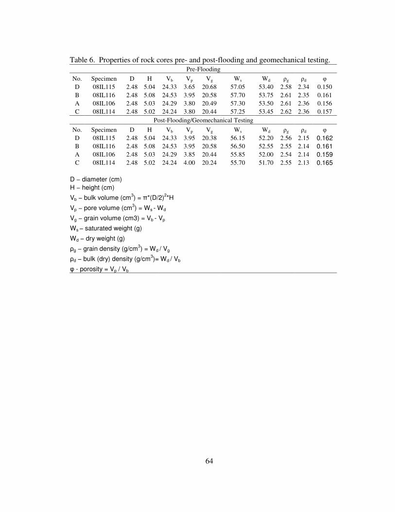
64

Table 6. Properties of rock cores pre- and post-flooding and geomechanical testing.

Pre-Flooding

No. Specimen D H Vb Vp Vg Ws Wd ρg ρd φ

D 08IL115 2.48 5.04 24.33 3.65 20.68 57.05 53.40 2.58 2.34 0.150

B 08IL116 2.48 5.08 24.53 3.95 20.58 57.70 53.75 2.61 2.35 0.161

A 08IL106 2.48 5.03 24.29 3.80 20.49 57.30 53.50 2.61 2.36 0.156

C 08IL114 2.48 5.02 24.24 3.80 20.44 57.25 53.45 2.62 2.36 0.157

Post-Flooding/Geomechanical Testing

No. Specimen D H Vb Vp Vg Ws Wd ρg ρd φ

D 08IL115 2.48 5.04 24.33 3.95 20.38 56.15 52.20 2.56 2.15 0.162

B 08IL116 2.48 5.08 24.53 3.95 20.58 56.50 52.55 2.55 2.14 0.161

A 08IL106 2.48 5.03 24.29 3.85 20.44 55.85 52.00 2.54 2.14 0.159

C 08IL114 2.48 5.02 24.24 4.00 20.24 55.70 51.70 2.55 2.13 0.165

D − diameter (cm)

H − height (cm)

Vb − bulk volume (cm3) = π*(D/2)

2*H

Vp − pore volume (cm3) = Ws - Wd

Vg − grain volume (cm3) = Vb - Vp

Ws − saturated weight (g)

Wd − dry weight (g)

ρg − grain density (g/cm3) = Wd / Vg

ρd − bulk (dry) density (g/cm3)= Wd / Vb

φ - porosity = Vp / Vb

65

Table 7: Sample IDs and corresponding sample descriptions. Each cycle represents

approximately 200 mL of CO2 injected, followed by 400 mL of saline or deionized water

injected.

Sample ID Sample Description Total Volume Injected, mL

(CO2 + H2O)

A 10,000 ppm stock solution 0

A1 10,000 ppm Cycle 1 600

A2 10,000 ppm Cycle 2 1200

A3 10,000 ppm Cycle 3 1800

A4 10,000 ppm Cycle 4 2400

A5 10,000 ppm Cycle 5 3000

AC 10,000 ppm CO2-DI 3000

B 1,000 ppm stock solution 0

B1 1,000 ppm Cycle 1 600

B2 1,000 ppm Cycle 2 1200

B3 1,000 ppm Cycle 3 1800

B4 1,000 ppm Cycle 4 2400

B5 1,000 ppm Cycle 5 3000

BC 1,000 ppm CO2-DI 3000

C 100,000 ppm stock solution 0

C1 100,000 ppm Cycle 1 600

C2 100,000 ppm Cycle 2 1200

C3 100,000 ppm Cycle 3 1800

C4 100,000 ppm Cycle 4 2400

C5 100,000 ppm Cycle 5 3000

CC 100,000 ppm CO2-DI 3000

D 0 ppm stock solution (DI) 0

D1 0 ppm cycle 1 600

D2 0 ppm cycle 2 1200

D3 0 ppm cycle 3 1800

D4 0 ppm cycle 4 2400

D5 0 ppm cycle 5 3000

DC 0 ppm CO2-DI 3000

66

Table 8: Dilution factors

Sample ID Na

+ Ca

2+ Fe

2+ Cl

- HCO3

- TDS

A 5,000 1 1 50 1 1

A1 5,000 100 1 50 1 1

A2 2,500 100 1 50 1 1

A3 2,500 50 1 50 1 1

A4 2,500 100 1 50 1 1

A5 5,000 10 1 50 1 1

AC 50 1 1 1 1 1

B 250 1 1 5 1 1

B1 250 50 1 5 1 1

B2 250 50 1 5 1 1

B3 250 50 1 5 1 1

B4 250 10 1 5 1 1

B5 250 10 1 5 1 1

BC 25 2 1 1 1 1

C 20,000 1 1 500 1 1

C1 20,000 100 1 500 1 1

C2 20,000 100 1 500 1 1

C3 20,000 100 1 500 1 1

C4 20,000 10 1 500 1 1

C5 20,000 100 1 500 1 1

CC 10,000 1 1 100 1 1

D 1 1 1 1 1 1

D1 1 25 1 1 1 1

D2 1 25 1 1 1 1

D3 1 25 1 1 1 1

D4 1 25 1 1 1 1

D5 1 25 1 1 1 1

DC 1 2 1 1 1 1

67

Table 9. Quality Control

Conc Conc Conc

Sample ID Ion SAM DUP SPK % dif % Rec.

A3D Ca 2.6334 2.6537 0.38

C1D Ca 4.2872 4.41447 1.46

DCD Na 1.2116 1.3089 3.86

A5D Ca 13.2763 14.2271 3.46

B3D Ca 4.446 4.7247 3.04

C4D Ca 14.6058 14.6042 0.01

A5D Ca 12.7401 13.1813 1.70

B3D Ca 4.2322 4.3928 1.86

C3D Ca 13.5077 13.5479 0.15

B3D Ca 4.2322 3.8238 5.07

A3D Na 1.4816 1.3568 4.40

ACD Na 0.1295 0.1137 6.50

C4D Na 1.9185 1.9509 0.84

A3D Fe 0.3442 0.3498 0.81

B2D Fe 0.0727 0.0782 3.64

C2D Fe 9.8906 9.8573 0.17

DCD Fe 0.1342 0.1509 5.86

D5D Na 1.042 1.0569 0.71

C4D Ca 16.9758 16.5303 1.33

A3D Ca 9.7899 10.1731 1.92

BD Cl 565.36 549.29 1.44

C3D Cl 59456.96 58404.01 0.89

D2D Cl 11.42 11.48 0.25

B3D Ca 7.9265 8.1842 12.2556 1.60 104.57

D5D Ca 3.6086 3.7367 9.3383 1.74 103.99

BCS Na 0.534 0.7334 129.95

AS Na 0.6931 0.9316 198.25

A4S Mg 0.9132 0.9426 100.14

BCS Na 0.5591 1.0285 98.37

A2S Fe 0.2321 1.4354 76.84

C5S Fe 1.5056 2.236 73.94

D4S Fe 0.0626 1.3319 77.41

C1S Fe 6.6351 6.6254 66.06

D4S Na 0.634 1.0459 93.49

C3S Ca 12.4951 16.4613 121.97

ACS Ca 8.0793 12.9997 114.20

D2S Cl 11.42 70.87 94.89

68

Table 10. Values for pH versus pore volume graph.

0 ppm 1,000 ppm 10,000 ppm 100,000 ppm

Vol pH Vol pH Vol pH Vol pH

750 6.98 754 6.78 745 6.72 745 6.53

747 6.96 749 6.72 740 6.70 742 6.52

743 7.10 742 6.73 733 6.68 738 6.60

740 6.96 734 6.70 726 6.71 735 6.60

737 6.91 727 6.78 720 6.72 732 6.64

734 6.56 719 6.70 713 6.76 728 6.67

731 6.67 712 6.84 707 6.78 725 6.63

727 6.86 704 6.76 700 6.78 722 6.57

724 7.09 697 6.72 694 6.80 718 6.49

721 7.05 689 6.82 687 6.80 715 6.41

718 6.86 682 6.89 681 6.80 711 6.48

714 6.95 674 6.87 675 6.78 708 6.66

711 6.79 667 6.93 668 6.74 705 6.62

708 7.02 659 6.89 662 6.68 701 6.62

705 6.74 651 5.75 655 6.20 698 6.65

702 7.14 644 4.90 649 4.72 695 6.67

698 6.71 636 5.18 644 4.76 691 6.67

695 6.99 628 5.02 632 4.82 688 6.65

692 6.90 621 5.15 627 4.49 684 6.59

689 7.28 616 5.21 623 4.85 681 6.59

685 7.36 611 5.30 611 4.68 678 6.61

682 7.25 603 5.21 604 5.01 674 6.59

679 7.33 596 5.23 596 6.91 671 6.54

676 6.95 588 6.97 594 6.71 668 6.55

672 7.00 583 6.82 584 6.69 664 6.47

669 7.28 577 6.80 577 6.69 657 5.74

666 6.59 570 6.82 571 6.71 655 4.76

663 6.14 564 6.80 564 6.73 651 4.75

660 4.89 558 6.90 558 6.76 647 4.59

654 5.15 551 6.82 551 6.76 643 4.65

652 4.90 545 6.86 545 6.78 639 4.61

650 5.09 538 6.91 538 6.75 636 4.61

648 4.70 532 6.92 532 6.72 632 4.61

644 5.00 525 6.92 526 6.69 628 4.68

640 5.21 519 6.96 519 6.48 627 4.60

637 4.19 512 6.88 513 5.90 624 4.60

633 4.11 506 6.65 506 5.64 620 4.65

629 4.41 499 4.68 500 4.75 616 4.62

627 5.09 492 4.69 497 4.65 613 4.66

625 5.04 487 5.15 494 4.57 609 4.78

621 4.53 479 4.45 475 4.73 605 6.41

618 4.40 472 4.63 473 4.64 601 6.64

614 5.21 466 4.51 464 4.57 599 7.54

610 4.40 460 5.28 456 4.89 599 7.42

606 6.54 453 4.65 449 6.27 599 7.28

603 6.68 447 7.18 446 6.27 599 6.87

69

Table 10, continued. Values for pH versus pore volume graph.

0 ppm 1,000 ppm 10,000 ppm 100,000 ppm

Vol pH Vol pH Vol pH Vol pH

601 6.87 444 7.26 445 6.26 596 6.82

599 6.79 441 6.93 443 6.15 592 6.85

596 6.57 435 6.88 434 6.17 589 6.85

593 6.56 428 6.92 427 6.17 586 6.86

589 6.86 422 6.87 421 6.21 582 6.86

586 6.50 415 6.89 414 6.25 579 6.86

583 6.64 409 6.89 408 6.23 576 6.84

580 6.92 402 6.98 401 6.25 572 6.82

576 6.91 396 6.97 395 6.27 569 6.82

573 6.63 390 7.00 389 6.27 565 6.82

570 6.91 383 6.89 382 6.30 562 6.83

567 6.89 377 6.89 376 6.29 559 6.79

564 6.66 370 6.86 365 6.32 555 6.79

560 6.99 364 5.64 363 6.71 552 6.83

557 6.83 357 3.71 356 6.11 549 6.83

554 6.77 350 4.95 350 4.74 545 6.86

551 6.81 343 4.49 343 4.60 542 6.85

547 6.85 341 4.19 343 4.39 538 6.83

544 7.04 334 4.98 329 4.73 535 6.82

541 6.77 326 5.02 322 4.72 532 6.79

538 6.70 324 4.95 321 4.47 528 6.82

534 7.08 316 4.47 310 4.73 525 6.75

531 6.83 309 5.04 294 6.33 522 6.80

528 6.65 301 7.08 293 6.30 518 6.76

525 6.73 297 7.35 293 6.18 515 6.45

522 6.96 293 7.03 283 6.19 511 4.58

518 6.81 287 7.02 276 6.21 505 4.76

515 6.57 280 6.96 270 6.23 501 4.73

512 5.81 274 7.01 264 6.23 494 4.63

509 4.86 267 7.01 257 6.27 490 4.62

500 4.63 261 6.99 251 6.26 486 4.63

500 5.03 255 7.02 244 6.27 482 4.61

499 4.31 248 7.03 238 6.28 479 4.61

498 5.12 242 7.04 231 6.33 475 4.64

494 4.67 235 7.06 225 6.35 471 4.58

490 5.24 229 7.07 218 6.38 467 4.61

486 5.25 222 7.03 212 6.46 464 4.62

483 5.05 216 7.01 205 6.81 460 4.59

479 4.80 208 6.92 203 6.51 456 4.62

479 4.47 200 4.50 203 6.08 452 4.86

475 5.02 194 4.50 199 4.39 449 6.64

471 5.08 186 4.57 192 4.51 445 7.47

468 4.96 179 4.98 183 4.36 443 6.82

464 5.20 171 3.87 175 4.52 440 6.83

460 7.07 167 4.83 173 4.24 436 6.83

456 7.05 159 4.22 170 4.44 433 6.83

70

Table 10, continued. Values for pH versus pore volume graph.

0 ppm 1,000 ppm 10,000 ppm 100,000 ppm

Vol pH Vol pH Vol pH Vol pH

453 6.94 152 5.61 158 3.89 430 6.84

451 6.93 144 7.37 151 6.25 426 6.85

448 6.91 142 7.05 149 6.17 423 6.87

445 7.03 136 7.05 148 6.20 420 6.87

442 6.85 130 7.03 148 6.24 416 6.86

439 6.96 123 6.99 142 6.23 413 6.86

435 7.00 117 7.06 136 6.27 409 6.86

432 7.10 110 7.01 129 6.28 406 6.84

429 6.91 104 7.05 123 6.31 403 6.85

426 6.89 97 7.05 116 6.36 399 6.85

423 6.90 91 7.07 110 6.35 396 6.86

419 7.11 84 7.06 104 6.36 393 6.85

416 7.13 78 7.08 97 6.42 389 6.86

413 7.10 71 6.97 91 6.43 386 6.88

410 7.08 65 6.93 84 6.47 382 6.88

406 7.12 59 6.80 78 6.63 379 6.91

403 7.12 53 6.54 71 6.82 376 6.88

400 7.07 47 3.61 65 6.43 372 6.88

397 7.20 44 4.20 61 4.29 369 6.84

394 7.09 41 3.97 48 4.45 366 6.74

390 7.11 34 3.86 40 4.09 362 6.50

387 7.17 28 3.49 33 4.33 359 6.37

384 7.08 20 3.73 25 4.11 355 6.43

381 6.93 13 3.75 21 3.99 352 7.21

377 7.02 5 6.44 16 4.45 349 4.66

374 6.86 345 4.67

371 6.84 344 4.54

368 7.21 342 4.57

365 6.19 339 4.57

361 4.59 335 4.58

353 4.86 331 4.55

351 4.61 329 4.57

348 3.98 328 4.54

344 4.22 327 4.58

340 3.73 324 4.56

336 3.71 320 4.59

333 4.82 316 4.61

329 4.95 312 4.68

328 3.43 309 6.45

324 4.32 305 6.78

320 4.47 302 7.55

317 3.64 299 7.12

313 3.49 297 7.04

309 6.54 289 7.09

305 6.90 282 7.10

302 7.07 274 7.11

71

Table 10, continued. Values for pH versus pore volume graph.

0 ppm 1,000 ppm 10,000 ppm 100,000 ppm

Vol pH Vol pH Vol pH Vol pH

299 6.92 267 7.11

297 7.03 259 7.13

293 6.99 252 7.03

290 6.92 244 7.03

287 7.07 237 7.01

284 7.13 229 6.99

281 7.10 222 6.78

277 6.94 215 5.96

274 6.80 207 5.22

271 7.03 200 4.55

268 7.16 185 4.56

264 7.01 180 4.56

261 6.97 174 4.56

258 7.08 167 4.59

255 7.21 159 4.67

252 7.23 152 7.48

248 7.14 151 7.37

245 7.05 151 7.07

242 7.18 151 7.02

239 7.27 144 7.05

235 7.25 136 7.06

232 7.26 129 7.04

229 7.20 121 7.03

226 6.94 114 6.99

222 7.04 107 6.98

219 7.17 99 6.96

216 6.30 92 6.92

213 4.58 84 6.80

210 4.59 77 6.26

205 3.77 70 4.31

202 5.95 62 4.34

180 3.81 50 4.44

179 3.97 43 4.33

178 3.94 37 5.16

175 3.78 29 4.16

171 3.79 22 4.22

168 4.88 14 4.07

164 3.40

160 5.11

156 6.80

152 7.07

150 6.92

147 7.04

144 6.94

140 6.96

137 6.95

72

Table 10, continued. Values for pH versus pore volume graph.

0 ppm 1,000 ppm 10,000 ppm 100,000 ppm

Vol pH Vol pH Vol pH Vol pH

134 6.96

131 6.87

128 7.02

124 6.97

121 7.04

118 6.88

115 7.03

111 6.88

108 6.97

105 7.02

102 6.84

99 6.85

95 6.95

92 6.99

89 6.92

86 6.92

82 6.87

79 6.80

76 6.85

73 6.39

66 7.48

63 4.37

60 4.46

55 4.98

51 4.92

47 4.98

43 4.79

39 4.59

36 4.38

32 3.76

28 4.82

27 4.23

25 4.60

21 4.06

18 4.54

14 4.71

10 4.69

6 4.74

3 5.91

73

Table 11. Values for conductance versus pore volume graph. Cond in mS/cm.

0 ppm 1,000 ppm 10,000 ppm 100,000 ppm

Volume Cond Volume Cond Volume Cond Volume Cond

750 0.530 749 2.590 745 17.530 745 127.800

747 0.534 742 2.586 740 17.730 742 127.900

743 0.536 734 2.600 733 17.350 738 126.600

740 0.545 727 2.616 726 17.250 735 126.600

737 0.541 719 2.637 720 17.420 732 126.400

734 0.541 712 2.653 713 17.320 728 126.900

731 0.560 704 2.674 707 17.250 725 126.900

727 0.575 697 2.665 700 16.710 722 126.900

724 0.582 689 2.344 694 16.660 718 126.900

721 0.592 682 2.405 687 14.800 715 126.900

718 0.600 674 2.461 681 14.800 711 126.600

714 0.610 667 2.519 675 14.360 708 126.400

711 0.621 659 1.478 668 8.027 705 125.000

708 0.632 644 0.344 662 3.547 701 121.300

705 0.625 636 0.343 649 0.668 698 120.100

702 0.633 628 0.336 644 0.720 695 107.200

698 0.576 621 0.326 632 0.667 691 107.200

695 0.593 616 0.324 627 0.612 688 107.200

692 0.620 611 0.321 623 0.600 684 106.500

689 0.648 603 0.319 611 0.591 681 104.400

685 0.676 596 0.313 596 17.980 678 89.630

682 0.711 588 2.814 594 17.860 674 68.980

679 0.756 583 2.807 584 17.870 671 45.410

676 0.715 577 2.819 577 17.770 668 8.048

672 0.481 570 2.840 571 17.800 661 0.001

669 0.332 564 2.869 564 17.920 655 6.550

660 0.210 558 2.892 558 17.840 651 6.500

654 0.220 551 2.921 551 17.120 647 6.491

652 0.220 545 2.847 545 16.960 643 6.480

650 0.220 538 2.862 538 15.030 639 6.478

648 0.219 532 2.585 532 15.040 636 6.467

644 0.219 525 2.651 526 14.720 632 6.409

640 0.217 519 2.511 519 7.647 628 6.346

637 0.220 512 1.677 513 0.018 627 6.325

633 0.212 506 0.253 506 0.001 624 6.350

629 0.212 492 0.295 500 0.546 620 6.315

627 0.212 487 0.296 497 0.546 616 6.296

625 0.212 479 0.292 494 0.558 613 6.319

621 0.210 472 0.289 475 0.501 609 6.316

618 0.210 466 0.295 473 0.501 605 130.000

614 0.210 460 0.290 464 0.478 601 129.600

610 0.209 453 0.283 456 0.467 599 129.300

606 0.724 441 3.016 449 18.220 599 129.200

603 0.726 441 3.014 446 18.370 599 128.100

601 0.727 441 3.035 445 18.190 599 126.300

599 0.723 435 3.043 443 17.840 596 130.300

74

Table 11, continued. Values for conductance versus pore volume injected graph.

Cond in mS/cm.

0 ppm 1,000 ppm 10,000 ppm 100,000 ppm

Volume Cond Volume Cond Volume Cond Volume Cond

596 0.727 428 3.072 434 17.880 592 130.300

593 0.732 422 3.080 427 17.650 589 130.300

589 0.743 415 3.099 421 17.750 586 130.300

586 0.755 409 3.120 414 17.660 582 130.300

583 0.762 402 3.009 408 17.730 579 130.300

580 0.770 396 2.680 401 17.680 576 130.000

576 0.776 390 2.718 395 16.890 572 130.000

573 0.793 383 2.755 389 14.830 569 129.900

570 0.805 377 2.151 382 15.070 565 129.900

567 0.816 370 0.777 376 14.830 562 129.900

564 0.828 364 0.006 365 9.877 559 129.300

560 0.843 343 0.228 363 0.004 555 128.100

557 0.853 341 0.227 356 0.006 552 122.500

554 0.844 334 0.226 350 0.519 549 108.500

551 0.855 326 0.225 343 0.420 545 108.100

547 0.868 324 0.224 343 0.416 542 108.300

544 0.803 316 0.221 329 0.416 538 108.300

541 0.824 309 0.218 322 0.423 535 107.800

538 0.858 301 3.242 310 0.406 532 107.300

534 0.901 297 3.222 294 17.910 528 105.300

531 0.952 293 3.197 293 17.860 525 88.700

528 0.999 287 3.218 293 17.440 522 62.910

525 0.925 280 3.252 283 17.540 518 27.560

522 0.696 274 3.284 276 17.680 515 0.312

518 0.536 267 3.323 270 17.600 511 0.022

515 0.437 261 3.377 264 17.690 505 6.005

509 0.207 255 3.391 257 17.670 501 6.006

500 0.193 248 3.323 251 17.620 494 6.060

500 0.192 242 3.362 244 17.450 490 6.029

499 0.194 235 3.067 238 15.070 486 6.045

498 0.192 229 3.175 231 15.040 482 5.690

494 0.191 222 2.550 225 14.970 479 5.661

490 0.192 216 1.317 218 13.830 475 5.652

486 0.188 200 0.182 212 7.091 471 5.628

483 0.184 194 0.200 199 0.003 467 5.644

479 0.175 186 0.202 192 0.356 464 5.655

479 0.175 179 0.177 183 0.348 460 5.624

475 0.174 171 0.065 175 0.267 456 5.619

471 0.173 167 0.174 173 0.260 452 5.467

468 0.171 159 0.175 170 0.235 449 127.300

464 0.170 152 0.162 158 0.211 445 126.900

456 0.997 144 3.180 151 0.161 443 128.400

453 1.004 142 3.139 149 17.870 440 128.500

451 1.060 136 3.158 148 17.510 436 128.700

448 1.072 130 3.189 148 17.840 433 128.700

75

Table 11, continued. Values for conductance versus pore volume injected graph.

Cond in mS/cm.

0 ppm 1,000 ppm 10,000 ppm 100,000 ppm

Volume Cond Volume Cond Volume Cond Volume Cond

445 1.079 123 3.229 142 18.040 430 128.500

442 1.091 117 3.268 136 18.180 426 128.500

439 1.114 110 3.324 129 18.120 423 128.500

435 1.131 104 3.378 123 18.110 420 128.300

432 1.151 97 3.431 116 18.120 416 128.300

429 1.158 91 3.400 110 17.940 413 128.300

426 1.183 84 3.169 104 17.740 409 128.200

423 1.211 78 3.282 97 17.000 406 128.100

419 1.232 71 3.318 91 15.180 403 127.700

416 1.253 65 2.402 84 14.780 399 126.400

413 1.280 59 1.388 78 13.750 396 122.100

410 1.293 47 0.120 71 8.593 393 121.200

406 1.277 49 0.118 65 0.122 389 108.100

403 1.300 41 0.118 48 0.148 386 108.100

400 1.300 34 0.110 40 0.139 382 107.600

397 1.230 28 0.109 33 0.125 379 106.600

394 1.266 20 0.108 25 0.108 376 101.700

390 1.324 13 0.105 21 0.104 372 80.570

387 1.382 5 0.086 16 0.094 369 59.270

384 1.439 9 0.048 366 35.150

381 1.413 362 1.691

377 1.123 355 0.010

374 0.905 349 5.407

371 0.670 345 5.410

368 0.257 344 5.359

361 0.179 342 5.382

353 0.162 339 5.369

351 0.160 335 5.345

348 0.162 331 5.357

344 0.161 329 5.329

340 0.161 328 5.329

336 0.159 327 5.326

333 0.139 324 5.293

329 0.139 320 5.285

328 0.139 316 5.253

324 0.139 312 5.234

320 0.139 309 130.400

317 0.137 305 130.200

313 0.137 302 130.000

309 0.129 299 127.800

305 1.061 297 127.700

302 1.069 289 127.500

299 1.074 282 127.500

297 1.146 274 127.500

293 1.165 267 126.900

76

Table 11, continued. Values for conductance versus pore volume injected graph.

Cond in mS/cm.

0 ppm 1,000 ppm 10,000 ppm 100,000 ppm

Volume Cond Volume Cond Volume Cond Volume Cond

290 1.174 259 121.600

287 1.192 252 120.700

284 1.209 244 106.300

281 1.228 237 105.200

277 1.250 229 67.060

274 1.269 222 0.339

271 1.289 200 4.854

268 1.312 185 4.861

264 1.339 180 4.861

261 1.346 174 4.879

258 1.347 167 4.812

255 1.374 159 4.506

252 1.412 152 127.100

248 1.448 151 127.600

245 1.345 151 126.300

242 1.409 151 127.100

239 1.449 144 126.700

235 1.453 136 126.600

232 1.219 129 126.100

229 1.046 121 120.300

226 0.884 114 119.200

222 0.665 107 103.700

219 0.128 99 103.400

213 0.130 92 81.010

210 0.128 84 30.660

205 0.121 77 26.120

202 0.121 70 0.002

198 0.146 62 1.521

195 0.146 50 1.470

191 0.146 43 1.401

187 0.146 37 1.205

183 0.146 29 1.170

180 0.150 22 1.051

179 0.104 14 0.882

178 0.103 6 0.258

175 0.102

171 0.098

168 0.094

164 0.092

160 0.089

156 1.236

152 1.244

150 1.276

147 1.288

144 1.314

77

Table 11, continued. Values for conductance versus pore volume injected graph.

Cond in mS/cm.

0 ppm 1,000 ppm 10,000 ppm 100,000 ppm

Volume Cond Volume Cond Volume Cond Volume Cond

140 1.337

137 1.354

134 1.377

131 1.398

128 1.426

124 1.448

121 1.481

118 1.509

115 1.546

111 1.570

108 1.531

105 1.414

102 1.453

99 1.495

95 1.542

92 1.619

89 1.691

86 1.786

82 1.873

79 1.850

76 1.225

73 0.164

63 0.085

60 0.085

55 0.084

51 0.085

47 0.082

43 0.078

39 0.073

36 0.075

32 0.067

28 0.065

27 0.064

25 0.065

21 0.063

18 0.062

14 0.061

10 0.054

3 0.012

78

Table 12. Water density calculations. Weight in g.

Soln. Wt. 1 mL Soln. Wt. 1 mL

0 0.9948 1000 0.9973

ppm 0.9928 ppm 0.9800

0.9861 0.9869

1.0114 0.9851

0.9865 0.9928

Average 0.9943 Average 0.9884

Soln. wt 1 mL Soln. wt 1 mL

10000 1.0034 100000 1.0619

ppm 1.0025 ppm 1.0557

0.9962 1.0533

1.0036 1.0547

1.0000 1.0542

Average 1.0011 Average 1.0560

79

APPENDIX C

Oil Fields in the Madison Group

80

ALEXANDER

ANTELOPE

ANTELOPE CREEK

ANTLER

ARNEGARD

ASSINIBOINE

AURELIA

AVOCA

BADEN

BAKER

BANKS

BANNER

BAR BUTTE

BARTA

BATTLEVIEW

BAUKOL NOONAN

BAUMANN DRAIN

BEAR CREEK

BEAR DEN

BEARS TAIL

BEAVER CREEK

BEAVER LODGE

BEICEGEL CREEK

BENNETT CREEK

BERG

BERTHOLD

BICENTENNIAL

BIG DIPPER

BIG STICK

BLACK SLOUGH

BLACKTAIL

BLAINE

BLUE BUTTES

BLUELL

BOUNDARY CREEK

BOWBELLS

BOWLINE

BOXCAR BUTTE

BRIAR CREEK

BROOKLYN

BUCKHORN

BUFFALO WALLOW

BUFORD

BULL BUTTE

BULL CREEK

BULL MOOSE

BULL RUN

BULLSNAKE

BUTTE

CABERNET

CAMEL BUTTE

CAMP

CAPA

CARTER

CARTWRIGHT

CATWALK

CEDAR CREEK

CENTENNIAL

CHARLSON

CHATEAU

CHOLA

CHURCH

CIMBEL

CLAY

CLAYTON

CLEAR CREEK

CLEAR WATER

COLQUHOUN

COLUMBUS

CORINTH

COTEAU

COULEE

COW CREEK

CRAZY MAN CREEK

CROFF

CROOKED CREEK

CROSBY

CULVER

CUSTOMS

CUTBANK CREEK

DALE

DANCE CREEK

DANEVILLE

DAVIS CREEK

DELTA

DES LACS

DEVILS PASS

DICKINSON

DIMMICK LAKE

DIMOND

DOLPHIN

DONNYBROOK

DORE

DRY CREEK

DUBLIN

DUCK CREEK

EAST FORK

EAST GOOSE LAKE

EAST TIOGA

EDEN VALLEY

EDGE

EIDSVOLD

EIGHTMILE

ELAND

ELK

ELKHORN RANCH

ELMORE

ELMS

ENTRY

EPPING

ESTES

FANCY BUTTES

FLAT LAKE EAST

FLAT TOP BUTTE

FLAXTON

FOOTHILLS

FOREMAN BUTTE

FOUR EYES

FRYBURG

FT. BUFORD

GARDEN

GAYLORD

GLASS BLUFF

GLENBURN

GOOD LUCK

GRASSLAND

GRASSY BUTTE

GREAT NORTHERN

GREEN LAKE

GREENBUSH

GREENE

GRENORA

GRINNELL

GROS VENTRE

GROVER

81

HAAS

HAMLET

HANKS

HARAM

HARDING

HARDSCRABBLE

HARTLAND

HAWKEYE

HAY CREEK

HAY DRAW

HAYLAND

HEART BUTTE

HEBRON

HEDBERG

HILINE

HOFFLUND

HULSE COULEE

HUNGRY MAN BUTTE

HURLEY

INDIAN HILL

IVANHOE

JOHNSON CORNER

KANE

KANU

KEENE

KILLDEER

KIMBERLY

KNUTSON

KUROKI

LAKE DARLING

LAKE ILO

LAKE TRENTON

LAKE VIEW

LAKESIDE

LANDA

LANSFORD

LARSON

LAST CHANCE

LEONARD

LESJE

LIGNITE

LINDAHL

LITTLE BUTTE

LITTLE DEEP CREEK

LITTLE KNIFE

LIVESTOCK

LOCKWOOD

LONE BUTTE

LONE TREE

LONESOME

LONG CREEK

LORAINE

LOST BRIDGE

LOSTWOOD

LUCKY MOUND

LUCY

MACKOBEE COULEE

MAD MAX

MANDAN

MANDAREE

MANNING

MARMON

MARQUIS

MARY

MCGREGOR

MCKINNEY

MEDORA

MIDDLE CREEK

MIDWAY

MINNESOTA

MISSOURI RIDGE

MOHALL

MONDAK

MORAINE

MORGAN DRAW

MOUNTROSE

MOUSE RIVER PARK

NAMELESS

NEW HOME

NIOBE

NOHLY LAKE

NOONAN

NORMA

NORTH BRANCH

NORTH ELKHORN

RANCH

NORTH GRANO

NORTH HAAS

NORTH MAXBASS

NORTH MOUSE RIVER

PARK

NORTH SERGIS

NORTH SOURIS

NORTH STAR

NORTH TIOGA

NORTH WESTHOPE

NORTHEAST FOOTHILLS

NORTHEAST LANDA

NORTHWEST MCGREGOR

NORWEGIAN CREEK

OAKDALE

OSLOE

PAINTED WOODS

PARK

PASSPORT

PATENT GATE

PAULSON

PERELLA

PERSHING

PICKETT

PIERRE CREEK

PLAZA

PLEASANT

PLEASANT VALLEY

POE

POKER JIM

PORTAL

POWERS LAKE

PRAIRIE JUNCTION

PRATT

PRESCOTT

PRONGHORN

RAGGED BUTTE

RANDOLPH

RAUB

RAWSON

RED WING CREEK

REFUGE

RENNIE LAKE

RENVILLE

RICHBURG

RIDER

RIVAL

ROCKY HILL

ROCKY RIDGE

82

ROOSEVELT

ROSEBUD

ROTH

ROUGH RIDER

ROUND TOP BUTTE

RUSSELL

RUSSIAN CREEK

SADDLE BUTTE

SADLER

SAKAKAWEA

SATHER LAKE

SCAIRT WOMAN

SCANDIA

SCOTIA

SERGIS

SEVENMILE COULEE

SHEALEY

SHERMAN

SHERWOOD

SHOCKLEY

SHORT CREEK

SIMON BUTTE

SIOUX

SIXMILE

SKABO

SMITH

SNOW

SNOWCOVER

SOURIS

SOUTH ANTLER CREEK

SOUTH BOXCAR

SOUTH BULL MOOSE

SOUTH COTEAU

SOUTH HAAS

SOUTH LANDA

SOUTH LONE TREE

SOUTH PLEASANT

SOUTH STARBUCK

SOUTH WESTHOPE

SOUTHWEST AURELIA

SOUTHWEST HAAS

SOUTHWEST LANDA

SOUTHWEST STARBUCK

SPIRAL

SPOTTED HORN

SPRING COULEE

SPRING VALLEY

SPRINGBROOK

SQUARE BUTTE

SQUAW CREEK

SQUAW GAP

ST. JACOBS

STADIUM

STAFFORD

STAMPEDE

STANLEY

STARBUCK

STINSON

STOCKYARD CREEK

STONEVIEW

STONY CREEK

STONY RUN

SUBDIVISION

SUGAR BEET

T. R.

TEMPLE

THOMPSON LAKE

TIMBER CREEK

TIOGA

TOBACCO GARDEN

TODD

TOLLEY

TORNING

TRAILSIDE

TREE TOP

TRURO

UKRAINA

UNION CENTER

UPPER DES LACS

VALLEY ROAD

VANVILLE

VERSIPPI

VIKING

WABEK

WAKE

WARD

WAYNE

WERNER

WEST BANK

WEST BUTTE

WEST CAPA

WEST DICKINSON

WEST GREENE

WEST ROTH

WEST SHERWOOD

WEST TIOGA

WESTHOPE

WHEATON

WHISKEY JOE

WHITE ASH

WHITE EARTH

WHITE LAKE

WILDROSE

WILEY

WILLIAMS CREEK

WILLISTON

WILLMEN

WILLOW CREEK

WINDMILL

WINTER BUTTE

WOBURN

ZION

83

REFERENCES

Allen, D., Strazisar, B., Soong, Y., Hedges, S. 2005. Modeling carbon dioxide

sequestration in saline aquifers: Significance of elevated pressures and salinities.

Fuel Processing Technology, 86 (14-15), 1569-1580.

Andre, L, Audigane, P, Azaroual, M., Menjoz, A. 2007. Numerical modeling of fluid-

rock chemical interactions at the supercritical CO2 liquid interface during CO2

injection into a carbonate reservoir, the Dogger aquifer (Paris Basin, France).

Energy Conversion Management, 48 (6), 1782-1797.

Bachu, S. 2000. Sequestration of CO2 in geological media: criteria and approach for site

selection in response to climate change. Energy Conversion Management, 41 (9),

953– 970.

Bachu, S. 2003. Screening and ranking of sedimentary basins for sequestration of CO2 in

geological media in response to climate change. Environmental Geology, 44 (3),

277– 289.

Bachu, S., Adams, J. 2003. Sequestration of CO2 in geological media in response to

climate change: capacity of deep saline aquifers to sequester CO2 in solution.

Energy Conversion Management, 44 (20), 3151–3175.

Bachu, S., Bonijoly, D., Bradshaw, J., Burruss, R., Holloway, S., Christensen, N.,

Mathiassen, O. 2007. CO2 storage capacity estimation: methodology and gaps.

International Journal of Greenhouse Gas Control, 1 (4), 430-443.

Bachu, S., Gunter, W., and Perkins, E. 1994. Aquifer disposal of CO2: Hydrodynamic

and mineral trapping. Energy Conversion Management, 35 (4), 269-279.

Bachu, S., Hitchon, B. 1996. Regional-scale flow of formation waters in the Williston

Basin. AAPG Bulletin, 80, 248–264.

Bateman, K., Turner, G., Pearce, J., Noy, D., Birchall, D., Rochelle, C. 2005 Large-Scale

Column Experiment: Study of CO2, Porewater, Rock Reactions and Model Test

Case. Oil & Gas Science and Technology – Rev. IFP, 60 (1), 161-175.

Bergman, P., Winter, E. 1995. Disposal of carbon dioxide in aquifers in the U.S. Energy

Conversion Management, 36 (6-9), 523-526.

84

Birkholzer, J., Zhou, Q., Tsang, C. 2009. Large-scale impact of CO2 storage in deep

saline aquifers: A sensitivity study on pressure response in stratified systems.

International Journal of Greenhouse Gas Control, 3 (2), 181-194.

Bluemle, J., Anderson, S., Andrew, J., Fischer D., LeFever, J., 1986. North Dakota

Stratigraphic Column, North Dakota Geological Survey. Miscellaneous Series

#66. Blunt, M., Fayers, F., Orr, Jr, F. 1993. Carbon dioxide in enhanced oil

recovery. Energy Conversion Management, 34 (9-11), 1197-1204.

Busby, J., Kimball, B., Downey, J., Peter, K. 1995. Geochemistry of water in aquifers

and confining units of the Northern Great Plains in parts of Montana, North

Dakota, South Dakota, and Wyoming. U.S. Geological Survey Professional

Paper 1402-F, p. F1-F146.

Carr, T., Wickstron, L., Korose, C., Fisher, R., Solano-Acosta, W., Eaton, N. 2003.

Online tools to evaluate saline aquifers for CO2 sequestration. Kansas Geological

Survey Open-File Report 2003-33.

Downey, J. 1984. Geohydrology of the Madison and associated aquifers in parts of

Montana, North Dakota, South Dakota, and Wyoming, U.S. Geological Survey

Professional Paper 1273-G, p. G1–G47.

Downey, J. 1986. Geohydrology of bedrock aquifers in the Northern Great Plains in

parts of Montana, North Dakota, South Dakota, and Wyoming, U.S. Geological

Survey Professional Paper 1402-E, p. E1–E87.

Downey, J. Dinwiddie, G. 1988. The Regional aquifer system underlying the Northern

Great Plains in parts of Montana, North Dakota, South Dakota, and Wyoming –

summary. U.S. Geological Survey Professional Paper 1402-A, p. A1-A64.

Duan, Z., Sun, R. 2003. An improved model calculating CO2 solubility in pure water and

aqueous NaCl solutions form 273 to 533 K and from 0 to 2000 bar. Chemical

Geology, 193 (3-4), 257-271.

Emberley, S., Hutcheon, I., Shevalier, M., Durocher, K., Mayer, B., Gunter, W., Perkins,

E. 2005. Monitoring of fluid-rock interaction and CO2 storage through produced

fluid sampling at the Weyburn CO2-injection enhanced oil recovery site,

Saskatchewan, Canada. Applied Geochemistry, 20 (6), 1131-1157.

Enting, I., Etheridge, D., Fielding, M. 2008. A perturbation analysis of the climate benefit

from geosequestration of carbon dioxide. International Journal of Greenhouse

Gas Control, 2 (3), 289-296.

Finneran, D., Morse, J. 2009 Calcite dissolution kinetics in saline waters. Chemical

Geology, 268 (1-2), 137-146.

85

Fischer, D., LeFever, J., LeFever, R., Anderson, S., Helms, L., Whittaker, S., Sorensen,

J., Smith, S., Peck, W., Steadman, E., Harju, J. 2005a. Overview of Williston

Basin Geology as it relates to CO2 sequestration. Plains CO2 Reduction

Partnership Report, University of North Dakota Energy and Environmental

Research Center, Grand Forks, North Dakota, USA.

Fischer, D., LeFever, J., LeFever, R., Helms, L., Sorensen, J., Smith, S., Steadman, E.,

Harju, J. 2005b. Mission Canyon Formation Outline. Plains CO2 Reduction

Partnership Report, University of North Dakota Energy and Environmental

Research Center, Grand Forks, North Dakota, USA.

Fischer, D., Smith, S., Peck, W., LeFever, J., LeFever, R., Helms, L., Sorensen, J.,

Steadman, E., Harju, J. 2005c. Sequestration potential of the Madison of the

Northern Great Plains aquifer system (Madison Geological Sequestration Unit).

Plains CO2 Reduction Partnership Report, University of North Dakota Energy and

Environmental Research Center, Grand Forks, North Dakota, USA.

Gaus, I., Audigane, P., Andre, L., Lions, J., Jacquemet, N., Durst, P., Czernichowski-

Lauriol, I., Azaroual, M. 2008. Geochemical and solute transport modeling for

CO2 storage, what to expect from it? International Journal of Greenhouse Gas

Control, 2 (4), 605-625.

Gerhard, L., Anderson, S., LeFever, J., Carlson, C. 1982. Geological development,

origin, and energy mineral resources of the Williston Basin, North Dakota. North

Dakota Geological Survey Miscellaneous Series 63. Bismarck, ND, USA.

Giammar, D., Bruant Jr., R., Peters, C. 2005. Forsterite dissolution and magnesite

precipitation at conditions relevant for deep saline aquifer storage and

sequestration of carbon dioxide. Chemical Geology, 217 (3-4), 257-276.

Gledhill, D., Morse, J. 2006. Calcite solubility in Na-Ca-Mg-Cl brines. Chemical

Geology, 233 (3-4), 249-256.

Grigg, R., Svec, R., Zeng, Z., Bai, B., Liu, Y. 2005. Improving CO2 efficiency for

recovering oil in heterogeneous reservoirs. Final report for DOE Contract No.

DE-FG26-01BC15364, New Mexico Petroleum Recovery Research Center,

Socorro, NM.

Gunter, W., Perkins, E., Hutcheon, I. 2000. Aquifer disposal of acid gases: modelling of

water–rock reactions for trapping of acid wastes. Applied Geochemistry, 15 (8),

1085– 1095.

Gunter,W., Wiwchar, B., Perkins, E. 1997. Aquifer disposal of CO2-rich greenhouse

gases: extension of the time scale of experiment for CO2-sequestering reactions

by geochemical modelling. Mineralogy and Petrology, 59 (1–2), 121– 140.

86

Hach Company. 2007. Alkalinity method 8203 by digital titrator, DOC316.53.01155,

Instrument Manual.

Heck, T. 1979. Depositional environments and diagenesis of the Mississippian Bottineau

Interval (Lodgepole) in North Dakota: University of North Dakota Unpublished

Master’s Thesis, p. 227.

Hem, J. 1985. Study and interpretation of the chemical characteristics of natural water.

USGS Water-Supply Paper 2254, p. 263.

Hitchon, B. 2000. ‘Rust’ contamination of formation waters from producing wells.

Applied Geochemistry, 15 (10), 1527-1533.

Hitchon, B., Gunter, W., Gentzis, T., Bailey, R. 1999. Sedimentary basins and

greenhouse gases: a serendipitous association. Energy Conversion Management,

40 (8), 825–843.

Holloway, S. 1997. An overview of the underground disposal of carbon dioxide. Energy

Conversion Management, 38 (SS), S193–S198.

Holloway, S., Savage, D. 1993. The potential for aquifer disposal of carbon dioxide in

the UK. Energy Conversion Management, 34 (9-11), 925-32.

Holtz, M., Nance, P., Finley, R. 2001. Reduction of greenhouse gas emissions through

CO2 EOR in Texas. Environmental Geosciences, 8 (3), 187-199.

Izgec, O., Demiral, B., Bertin, H., Akin, S. 2008. CO2 injection into saline carbonate

aquifer formations I: laboratory investigation. Transport in Porous Media, 72 (1),

1-24.

Jiang, C., Li, M., Osadetz, K., Snowdon, L., Obermajer, M., Fowler, M. 2001.

Bakken/Madison petroleum systems in the Canadian Williston Basin. Part 2:

molecular markers diagnostic of Bakken and Lodgepole source rocks. Organic

Geochemistry, 32, 1037-1054.

Kaszuba, J., Janecky, D., Snow, M. 2003. Carbon dioxide reaction processes in a model

brine aquifer at 200 °C and 200 bars: implications for geologic sequestration of

carbon. Applied Geochemistry, 18 (7), 1065-1080.

Kaszuba, J., Janecky, D., Snow, M. 2005. Experimental evaluation of mixed fluid

reactions between supercritical carbon dioxide and NaCl brine: Relevance to the

integrity of a geologic carbon repository. Chemical Geology, 217 (3-4), 277-293.

87

Ketzer, R., Iglesias, R., Einloft, S., Dullius, J., Ligabue, R., de Lima, V. 2009. Water-

rock-CO2 interactions in saline aquifers aimed for carbon dioxide storage:

Experimental and numerical modeling studies of the Rio Bonito Formation

(Permian), southern Brazil. Applied Geochemistry, 24 (5), 760-767.

Kharaka, Y., Thordsen, J., Hovorka, S., Nance, H., Cole, D., Phelps, T., Knauss, K.

2009. Potential environmental issues of CO2 storage in deep saline aquifers:

Geochemical results from the Frio-I Brine Pilot test, Texas, USA. Applied

Geochemistry, 24 (6), 1106-1112.

Lagneau, V., Pipart, A., Catalette, H. 2005. Reactive transport modelling of CO2

sequestration in deep saline aquifers. Oil Gas Science and Technology, 60 (2),

231–247.

Law, D., Bachu, S. 1996. Hydrogeological and numerical analysis of CO2 disposal in

deep aquifers in the Alberta Sedimentary Basin. Energy Conversion

Management, 37 (6-8), 1167-1174.

LeFever, J., LeFever R. 2005. Salts in the Williston Basin, North Dakota. NDGS Report

of Investigations No. 103.

LeFever, R. 1998. Hydrodynamics of Formation Waters in the North Dakota Williston

Basin. Eighth International Williston Basin Symposium, Saskatchewan

Geological Society Special Publication No. 13, p. 229-237.

LeFever, R. 2009. Personal Correspondence.

McGee, E. 1989. Mineralogical Characterization of the Shelburne Marble and the Salem

Limestone – Test Stones Used to Study the Effects of Acid Rain. U. S.

Geological Survey Bulletin, Report: B 1889, p. 25.

Nelms, R., Burke, R. 2004. Evaluation of oil reservoir characteristics to assess North

Dakota carbon dioxide miscible flooding potential. 12th

Williston Basin

Horizontal Well and Petroleum Conference May 2-4, Minot, ND, USA.

Oruganti, Y., Bryant, S. 2009. Pressure build-up during CO2 storage in partially

confined aquifers. Energy Procedia, 1 (1), 3315-3322.

Pawar, R., Zhang, D., Westrich, J., Grigg, R., and Stubbs, B. 2002. Geological

Sequestration of Carbon Dioxide in a Depleted Oil Reservoir. Paper 75256

presented at the SPE/DOE Thirteenth Symposium on Improved Oil Recovery,

Tulsa, April 13-17, 2002.

88

Portier, S., Rochelle, C. 2005. Modelling CO2 solubility in pure water and NaCl-type

waters from 0 to 300 °C and from 1 to 300 bar Application to the Utsira

Formation at Sleipner. Chemical Geology, 217 (3-4), 187-199.

Preston, C., Monea, M., Jazrawi, W., Brown, K., Whittaker, S., White, D., Law, D.,

Chalaturnyk, R., Rostron, B. 2005. IEA GHG Weyburn CO22 monitoring and

storage project. Fuel Processing Technology, 86 (14-15), 1547-1568.

Qi, R., LaForce, T., Blunt, M. 2009. Design of carbon dioxide storage in aquifers.

International Journal of Greenhouse Gas Control, 3 (2), 195-205.

Rosenbauer, R., Koksalan, T., Palandri, J. 2005. Experimental investigation of CO2–

brine–rock interactions at elevated temperature and pressure: Implications for

CO2 sequestration in deep-saline aquifers. Fuel Processing Technology, 86, 1581–

1597.

Shiraki, R., Dunn, T. 2000. Experimental study on water–rock interactions during CO2

flooding in the Tensleep Formation, Wyoming, USA. Applied Geochemistry, 15

(3), 265–279.

Smith, N. 1966. Sedimentology of the Salem Limestone in Indiana. The Ohio Journal of

Science, 66 (2) 168-179.

Solomon, S., Carpenter, M., Flach, T. 2008. Intermediate storage of carbon dioxide in

geological formations: A technical perspective. International Journal of

Greenhouse Gas Control, 2 (4), 502-510.

Soong, Y., Goodman, A., McCarthy-Jones, J., Baltrus, J. 2004. Experimental and

simulation studies on mineral trapping of CO2 with brine. Energy Conversion

Management, 45 (11-12), 1845–1859.

Spycher, N., Pruess, K. 2005. CO2-H2O mixtures in the geological sequestration of CO2.

II. Partitioning in chloride brines at 12-100 °C and up to 60 bar. Geochimica

Cosmochimica Acta, 69 (13), 3309-3320.

Taku Ide, S., Jessen, K., Orr Jr, F. 2007. Storage of CO2 in saline aquifers: Effects of

gravity, viscous, and capillary forces on amount and timing of trapping.

International Journal of Greenhouse Gas Control, 1 (4), 481-491.

Testamale, D., Dufaud, F., Martinez, I., Bénézeth, P., Hazemann, J. Schott, J., Guyot, F. 2009.

An X-ray absorption study of the dissolution of siderite at 300 bar between 50°C and

100°C. Chemical Geology, 259 (1), 8-16.

U.S. Department of Energy, 2002. CO2 capture and storage in geologic formations. A

white paper prepared for the National Climate Change Technology Initiative.

89

van der Meer, L. 1993. The conditions limiting CO2 storage in aquifers. Energy Conversion

Management, 34 (9-11), 959-966.

Weir, G., White, S., Kissling, W. 1995. Reservoir storage and containment of

greenhouse gases. Energy Conversion Management, 36 (6-9), 531-534.

Xu, T., Apps, J., Pruess, K. 2004. Numerical simulation of CO2 disposal by mineral

trapping in deep aquifers. Applied Geochemistry, 19 (6), 917–936.

Yang, D., Gu, Y., Tontiwachwuthikul, P. 2008. Wettability determination of the reservoir

brine-reservoir rock system with dissolution of CO2 at high pressures and elevated

temperatures. Energy & Fuels, 22 (1), 504-509.

Zeng, Z. 2006. Multipurpose tri-axial core flooding system. Research Report.

University of North Dakota, Grand Forks, ND, USA.

Zhou, Q., Birkholzer, J., Tsang, C., Rutqvist, J. 2008a. A method for quick assessment of

CO2 storage capacity in closed and semi-closed saline formations. International

Journal of Greenhouse Gas Control, 2 (4), 626-639.

Zhou, X., Zeng, Z., and Belobraydic, M., Han, Y. 2008b. Geomechanical stability

assessment of Williston Basin formations for petroleum production and CO2

sequestration. 42nd

US Rock Mechanics Symposium and 2nd

U.S.-Canada Rock

Mechanics Symposium, June 29-July 2, San Francisco, CA.

Zhou, X., Zeng, Z., Liu, H., Boock, A. 2009. Laboratory testing on geomechanical

properties of carbonate rocks for CO2 sequestration. 43rd

US Rock Mechanics

Symposium and 4th

U.S.-Canada Rock Mechanics Symposium, June 28-July 1,

Asheville, NC.