capitat - Virginia Tech-Northern Virginia Center Data Identification Methods in... · IEEETransactions on PowerApparatus and Systems, Vol. PAS-104, No. 11, November 1985 BAD DATA

IEEE Transactions on Power Apparatus and Systems, Vol. PAS-104, No. 11, November 1985

BAD DATA IDENTIFICATION METHODS IN POWER SYSTEM STATE ESTIMATION - A COMPARATIVE STUDY

Th. Van Cutsem M. Ribbens-Pavella

Department of Electrical Engineering; University of LiegeSart-Tilman, B- 4000 Liege, Belgium

Abstract - The identification techniques available todayare first classified into three broad classes. Theirbehaviour with respect to selected criteria are thenexplored and assessed. Further, a series of simulationsare carried outwith various types ofbad data. Investig-ating the way these identification techniques be-have allows completing and validating the theoreticalcomparisons and conclusions.

la INTRODUCTIONIn the list of a power system state e3timator soft-

ware routines, bad data identification is the last -

but not least - satellite function. Its task is to

guarantee the reliability of the data base generatedthrough the estimator. Indeed, despitethe preprocessingdata validation techniques used to clear the data re-

ceived at a control center, gross anomalies (suchas baddata, modelling and parameter errors) may still existduring estimation. To avoid corrupting the resultingdata base, it is of great importance that these anoma-

lies are identified and further eliminated from the setof measurements. This explains why the need for a func-tion capable to identify bad data has been felt almostsimultaneously with the need for the state estimationfunction itself. It also explains the number and diver-sity of research works carried out on the subject.

This paper aims at providing a comparative assess-

ment of the "post-estimation" identification methods(1)available today. More specifically it concentrates on

evaluating the techniques able to identify bad data(BD), i.e. grossly erroneous measurements. These tech-niques are first classified, then explored and compared.Three broad classes are distinguished : the class ofidentification by elimrrnation (IBE) (1-14], that of thenon-quadratic criteria (NQC) [3,15-20], and the hypo-thesis testing identification (HTI) [211. The investi-gations are based upon both theoretical considerationsand practical experience. The latter has been acquiredthrough simulations performed on four different power

systems. The results reported here concern simulationsperformed on the IEEE 30-bus system, with the threepossible types of multiple BD : noninteracting, inter-acting, and unidentifiable ones.

The paper is organized as follows. Section 2gathers the material necessary for the intended explo-ration. The reader is supposed to be familiar at leastwith state estimation and BD detection techniques; so

this Section focuses essentially on topological identi-fiability aspects and selection of identifiabilitycriteria. Section 3 gives a brief description of thevarious identification methods within their correspond-ing categories,while Section 4 investigates further andcompares the three main methodologies. Finally, the ex-

ploration is completed and validated through the simu-lation results of Section 5.

85 WM 060-9 A paper recommended and approvedby the IEEE Power System Engineering Committee of

the IEEE Power Engineering Society for presentationat the IEEE/PES 1985 Winter Meeting, New York, New

York, February 3 - 8, 1985. Manuscript submitted

January 19, 1984; made available for printingNovember 19, 1984.

2, MISCELLANIESSomewhat hybrid, this Section groups the various

pieces of information necessary for the subsequentdevelopments. The degree of the authors' personal per-ception and interpretation goes increasing along the

paragraphs. Starting with definitions of the usual

symbols in § 2.1, one is led up to some useful topo-logical considerations and definitions in § 2.3 and 2.4

and finally to the selection of relevant identifiabilitycriteria to be used in the comparative assessment of

the various identification methodologies.

2.1. STATE ESTIMATION: DEFINITIONS AN SYMBOLS

N. B. With ome obviouz exception2, foweL ca6e ita&&cZetteA6 indicate vecto4, czapita ittc and capitatG'teek tetteA denote maticea.

One seeks the estimate I of the true state x whichbest fits the measurements z related to x through the

model : a 4 (_ 1)

where the customary notation is used:z : the m-dimensional measurement vector;x : the n-dimensional state vector of voltage mag-

nitudes and phase angles;n = 2N- 1, N being the number of system nodes;e the m-dimensional measurement error vector;

its i-th component is2:- a normal noise N(0,Ui) if the correspondingmeasurement is valid,

- an unknown quantity otherwise.

Moreover use will be made of the variable

ei vi- E[eiJ , where E stands for expectation.

The weighted least squares (WLS) estimate

satisfies the optimality condition

HT(.1) R- [z- h(±)I = HT(e) R 1 r = 0 (2)

where HA ah/ax denotes the Jacobian matrix,R= diag (at) and the measurement residual vector is bydefinition . A -A I

where W= IBEHTR 1 and E - (HTR-lH)1 (3')

In the absence of BD, the measurement residualvector is distributed : N(0,WRWTT)= N(O,WR)

The presence of BD is currently detected throughone of the variables below :

the weighted residual vector rW = /R-rr (4)

- the normalized residual vector

rN = r with D = diag(WR) (5)

- the quadratic cost function

J(e) = rTR-U r =rWrW (6)

2.2. DETECTABILITY OF BAD DATA

For any detection test, the probability 6 of non-

detecting BD is given by

6 = prob (ji|<X)

(*) On leave from "Socidt6 Tunisienne de l'Electricitdet du Gaz" (STEG), Tunis, Tunisia.

(1) The term "post" is used to clearly differentiate

the identification methods of concern here from the

preprocessing data validation techniques which are

beyond the scope of this paper.

0018-9510/85/1100-3037$01.00©1985 IEEE

L. Mili (*)

3037

z=-i4k;4' t e % JL

r _= z- n tx) = we t i )

Authorized licensed use limited to: to IEEExplore provided by Virginia Tech Libraries. Downloaded on January 16, 2010 at 13:31 from IEEE Xplore. Restrictions apply.

3038

where ; is the statistical variable of concern (rwi,rNi or J ) with meanvalue 1p and variance C2 ; X is thedetection threshold. Hence,detecting the presence of BDrequires that [241 |1| > X-N(N7)Let us now consider the case of a single BD.Definition. Given an error probability B, the detecta-b-iZlity threshold of the i-th measurementis defined asthe minimal magnitude of the corresponding weightederror e! necessary to detect the presence of BD with a

probability Pd= 1-S of success (the other measurementsbeing affected by gaussian noises).

Fig. 1 shows the value of the relative detectabilitythreshold corresponding to the rw, rN and J tests as

a function of the Wii coefficient. These curves, plot-ted via eq. (7) ,- inspire the following comments(i) in presence of a single BD (and in the absence of"critical pairs" [21]), the most powerful test is theone based on rN; recall moreover that within the linear-ized approximation and provided that ej = 0 (Vj # i), thelargest normalized residual, IrNilmax, corresponds tothe erroneous measurement. This is generally not truefor IrW. Imax * Hence the advantage of relying on normal-ized rathIr than on weighted residuals;(ii) when the local redundancy decreases, Wii decreases too;,hence, in order to be detectable, the errors must be larger;(iii) critical measurements are characterized by Wii= 0:their errors are thus undetectable. Indeed such measure-

ments have always null residuals;(iv) in the presence of riultiple BD, property (i) doesnot hold anymore. Indeed, in this case, E[rNi] is a

linear combination of the gross errors (e.g. see (2.11)in [211);(v) despite the above risk of erroneous judgement, therN criterion still remains the most reliable one; it willtherefore be used to determine the suspected measure-ments : these are measurements possessing normalizedresiduals larger than the fixed threshold.

2.3. TOPOLOGICAL IDENTIFIABILITY OF BAD DATA

Given a set of BD it is interesting to determinewhether the measurement configuration is rich enough toallow their proper identification.Definition. A set of BD is said to be topoZogicaZZyidentifiable if their suppression does not cause- system's unobservability,- creation of critical measurements.Proposition. To be identifiable a set of BD must neces-

sarily be topologically identifiable.

This proposition expresses the following evidencein order to identify f BD among m' measurements, it isnecessarythat f < m'-n' , where n' is the number of unknowstobe estimated. Note that this is a necessary but not suffi-cient condition for proper identification; indeed numer-

ical aspects have also to be taken into account.A reliable identification procedure should be able

to recognize topologically unidentifiable BD; in suchcases, it should declare the problem unsolvable and warnthe operator against the lackof reliabilityof the avail-able state estimate, rather than give unusable results.

2.4. MEASUREMENTS BECOMING CRITICAL DURING ELIMINATION

Identification methods based on (successive) elimin-ations of measurements may lead to situations where theremaining measurements are critical : the detection testsare then negative, since errors on critical measurementsare undetectable. Now it is possibZe that errors remainon these critical measurements, which would heavilyaffect the accuracy of the final state estimate (the re-

maining errors being no longer filtered). In such casesneither of the first two objectives of § 2.5 is attained.

Note that new critical measurements may be gener-ated because of:- the presence of topologically unidentifiable BD,- the undue elimination of valid measurements.

w - a is the false° alarm probability0 02 0.4 0.6 0.8 1.0

Fig. 1: Detectability threshoZds vs. WijIn order to enhance the reliability of the final

data base, we propose the following post-eliminationprocedure :(i) search for all measurements become critical afterelimination;(ii) add these critical measurements to the list of themeasurements declared false;(iii) determine the estimates which would be affectedbypossible errors on the critical measurements and jointhis qualitative information to the final data base.

Step (i) can be carried out by simply comparingthelists of critical measurements before and after elimina-tion.

The above procedure may apply to any identificationmethod which involves elimination of measurements.

2.5. PERFORMANCE ASSESSMENT CRITERIA

Five criteria are selected for assessingthe qualityof the various identification methods. The first threeof them are the main objectives sought by any identifi-cation approach as such. The two others concernits prac-tical feasibility, i.e. the applicability requirements.

LocacUzation oi the BV : ability to localize exact-ly the BD, or at least to furnish a list of suspectedmeasurements which includes all the BD and as few aspossible valid data.

Cotection oJ _the_na.t datao bae : the aptitudefor clearing the final data base is of great practicalimportance and one of the most essential tasks of theoverall state estimation process.

ReoSoniio o_pagegcay_undentieabte BD:whenever such BD arise, the algorithm should be able todraw up an as reduced as possible list of suspected mea-surements while containing all the BD; moreoverit shouldwarn the operator of its unability to identify the sus-pected data which have become critical and thereby thepossible existence of erroneous estimates rather thanprovide him with misleading results.

Tmptementation_&eqyWLemients : practical consider-ations on the implementation and design should be takeninto account, such as simplicity, adaptabilityto systemmodifications; to a lesser extent, memory storage.

Compy,textVe it should be as short as possibleso as to comply with the real-time requirements of theoverall operation.

3. BAD DATA IDENTIFICATION. BRIEF OVERVIEWTwo criteria are used to classify the various BD

identification methods :- the nature of the statistical tests of concern, deter-mined by the variables they imply,

- the way of eliminating BD and clearing the data base.The first criterion leads to distinguish HTI from theother methods, whereas the second leads to regroupingthe various nonquadratic criteria in a class distinctfrom that of the elimination procedures.


3.1. IDENTIFICATION BY ELIMINATION (IBE)

Conceptually, this identification is the continua-tionof theBD detection step which is a global criterionimplying the residual vector r . The leading idea isthat in the event of a positive detection test, a firstlist of candidate BD is drawn up on the basis of an rN(or rW ) test, then successive cycles of elimination-reestimation-redetection are performed until the detec-tion test becomes negative.

Two subclasses may be distinguished correspondingto the elimination of single or of grouped BD. Intro-duced by Schweppe et al. [1] almost at the same timewith the state estimation itself, the former consistsin eliminating at each cycle the measurement having thelargest magnitude of the normalized or weighted residu-al. As for the grouped elimination, a grouped residualsearch has been proposed by Handschin et al. [31; itconsists in eliminating a group of suspected measure-ments which supposedly includes all BD, and reinsertingthem afterwords one-by-one.

Another variant of these procedures consists insolving eqs. (3) with respect to one or several suspectedmeasurement errors, then in correcting them by substract-ing these errors. This measurement error estimation hasfirst been proposed by Aboytes and Cory [6]. Later on,Garcia et al. [7,8] have explored the simplified way ofcorrecting one measurement at a time (the one having ateach step the largest IrNil ) and keeping the W matrixconstant during the subsequent computations of rN. Notethat this technique has also been applied by Simoes-Costa et al. [14] to the orthogonal row processingsequential estimator. The work by Xiang Nian-de et al.[9-11] has significantly contributed to elucidate thisquestion. These authors have brought up the singularcharacter of W , have proposed its partitioning so asto estimate only s (s< m-n) out of the m measurementerrors. Moreover, they have clearly pointed outthe factthat correcting these s measurements amownts to eZimin-ating them. Attempting to improve this technique, MaZhi-quiang proposed to process combinatorial sets of sus-pected measurements and to identify the BD through adetection test based on an interesting formula he estab-lished in Ref. [121 (see § 4.1. 3 below). Now, becauseofthe equivalence between correction and elimination, thefact remains that all these techniques belong to theclass of the procedures by elimination.

3.2. NON QUADRATIC CRITERIA (NQC)

Almost in parallel with the above approach, theNQChave started being developed and explored. The idea ofthis methodology differs totally from the preceding one:here the identification-elimination of BD is part of thestate estimation itself. The rejection of the suspectedmeasurements depends upon the magnitudes of the (normal-ized or weighted) residuals : the larger the residual,the smaller the weight allocated to the correspondingmeasurement, and the larger the degree of its rejection.

Initiated by Merril and Schweppe [151 the NQC meth-ods have been further developed and analyzed by Handschinet al.[3] and by Muller [171. More recently, a compara-tive study of some of them has been carried out by Lo etal.[191 and by Falcao et al.[20].3.3. HYPOTHESIS TESTING IDENTIFICATION (HTI)

Unlike the two previous methodologies, HTI uses in-dividual criteria, particularized to each suspected mea-surement. The variables of concern here are the errorestimates, es , of some of the suspected measurements;these are evaluated through a suitable partitioning ofeq.(3) and a linear estimation. Exploiting the statis-tical properties of each e through an individualidentification testing allows deciding whether the cor-responding measurement is erroneous or not. This methodalong with two strategies for taking decisions is devel-oped in Ref.[21].

3039

4. BAD DATA IDENTIFICATION. CRITICAL. ANALYSIS

4.1. IDENTIFICATION BY ELIMINATION (IBE)

4.1.1. Description

The methods of this class rely on the rW or therN test. The choice between rW and rN implies a trade-off between good applicability features (simplicity,timeand core savings) and reliability. Generally, the poorperformances of rW (apart from the special caseof highredundancy and single BD) make the rN test worth-con-ceding the additional implementation effort. Neverthe-less, the latter is not reliable enough either; indeed,in case of multiple interacting BD, the one-to-one cor-respondence between largest IrN and erroneous mea-surement stops being guaranteed : valid measurementsmay thus be declared false and vice-versa.

Note that the decision is taken on a global basisgiven by the sole detection test, which just informsabout the existence of BD among the measurements, butdoes not indicate whether the eliminated ones are actu-ally erroneous.

4.1.2. Assessment

Puos* it is simple, since the only computation it needs be-

sides estimation is that of residuals;* it is capable to warn the operator that the BD are

topologically unidentifiable, provided the method of§ 2.4 is implemented.

* it is heavy since it requires a series of reestima-tion-detection after each elimination; this may leadto computer times incompatible with the on-line re-quirements;

* it may lead to a degradation of the measurement con-figuration and a subsequent drop of the power of thedetection test (see fig.1); thisin turnmay cause animportant probability of non-detecting remaining BD(especially when they become critical);

* it can provoke an undue elimination of valid measure-ments causing not only a rough identification butalso a drop of the detection test power. When usingthe rN test, this situation arises in the case ofmultiple interacting BD or of BD located in regionswith low local redundancy, i.e. in the case of strin-gent identification conditions. On the other hand,the rw test may lead to a degradation even in mildsituations.

4.1.3. Remarks on the correction of measurements

Within the procedure by elimination, two variantsmay be distinguished. The first consists in correcting,after each reestimation, the measurement having thelargesttrNi[ by substracting from its value the esti-mate e -1

ei = wi ri (8)1 ii1while keeping constant the W matrix.

The second variant consists in correcting a groupof s selected measurements among the suspected ones bysubtracting from their values the estimates

where : es =W5e rs = rr5 (9)s : denotes the selected measurements,

is the corresponding (s Xs) -dimensional sub-matrix of W

rs : is the corresponding s-dimensional subvector ofr..To avoid successive reestimations of the state

vector,the following correction formula of J(') pro-posed by Ma Zhi-quiang [12] can be used

J(XC)= J(x) -srs es ' (10)

Here xc is the new state vector obtained from the mea-

surements corrected by es (i.e. eliminated). Therefore,2

J xc has a x _distribution with (m-n-s) degrees offreedom.


3040

The advantages and drawbacks of the above tech-niques are summarized hereafter.PU4o* The main attractiveness of these techniques is that

the correction does not affect the measurement con-figuration. Hence, the gain matrix can be kept con-stant during the successive reestimations of the wholeidentification procedure, while keeping the goodnessof the minimization procedure convergence. On the con-trary, eliminating BD may deteriorate this convergence.It may even happen that such a procedure which con-verges properly through the above technique, divergeswhen eliminating the BD.

ConsIn addition to the weaknesses of thevery procedure

by elimination listed above, these correction techniquesinduce the following disadvantagesAs for the single correction-elimination* there is a risk that some measurements previously cor-

rected become erroneous again. Indeed, in order thatcorrection and elimination to be equivalent at eachstep, all the (s-1) previously corrected measurementsmust be corrected again along with the lastone througheq. (9) (see Ref. [21]);

* there is a greater risk to declare false a valid mea-surement because of the approximation of the normal-ized residual. Indeed, the variances of the residualscomputed on the basis of the initial W matrix are nolonger valid since the residuals of the non correctedmeasurements are equal to those resulting from theactual elimination of the corrected measurements andthe residuals of the corrected ones are zero (if thecorrection is carried out only through eq. (10)).

Concerning the grouped correction-elimination* the computation time may increase significantly (and

even become prohibitive with the number of times thelinear system given by (8) and (9) is solved), even ifa grouped residual search is used.

4.2. IDENTIFICATION BY NWC4.2.1. Description

The NQC methodology consists in minimizing the costfunction m

J (x) = fi (ri/ai) (1 1)i=1

where fi is equal to rl/4G when IrXi <Y ; here rX,denotes either rW. or rNi and y is a properly chosenthreshold. When IrXi|Y fi takes one of the follow-ing criteria [3]: quadratic-tangent (QT), quadratic-linear (QL), quadratic-square root (QR), quadratic-con-stant (QC), etc.

Applying the Gauss-Newton algorithm to minimize(11) gives the following iterative algorithm [3,171

HTP H [x (Q+1)-x(t)] =H Q [z -h(x(9))] (12)

where P and Q are diagonal weighting matrices depend-ing on the residuals. The comparison of eq. (12) withthecorresponding basic WLS algorithm (P Q=R-1) showsthat the method consists in modifying the weights of themeasurements according to their residuals. Fig. 2 indi-cates the variation of the weight Qii with the magni-tude of the corresponding residual. As can be seen, thelarger Ithe Irwi (resp. IrNi ),the stronger the re-jection of the corresponding measurement. This figurecompares also the rejection effect of the variouscriteria. In particular, the QC criterion is a border-line case, since it purely eliminates those mesurementswhose residuals are larger than y . Therefore minimizingthe QC criterion amounts to eliminating and/or reinsert-ing measurements at each iteration.

4.2.2. Assessment

PUZb. The main advantage of the NQC method lies in itssimplicity. Indeed, on one hand, it can be implementedthrough a simple transformation of the basic WLS algo-

0 2 4 6 8 10

FIG. 2: variation of Qiij vs. rWi /yrithm; on the other hand, the estimation and identifica-tion steps are carried out in a single procedure, whichavoids successive reestimations.Com6. The method suffers from the following seriousdrawbacks.* Possible existence of local minima : this, however,can be circumvented by using as a starting point theresult of a WLS estimation.* Strong tendency to slow convergence or even to di-vergence: the NQC exhibit a slower convergence than thecorresponding quadratic criterion. This can be explainedas follows- the shape of the cost function is more intricate;- the rejection of many measurements may lead to numer-

ically unobservable situations, especially in cases ofpoor local redundancy and/or multiple interacting BD.

* High risk of wrong identification. Schematically,the NQC rely on measurements having small residuals(with respect to y ) and tend to reject the others. Now,since there is no one-to-one correspondence betweenlarge residuals and large measurement errors (see§ 4.1)it may happen that valid measurements are rejectedwhereas erroneous ones are kept. In such a case the es-timate is much less reliable than that givenby the qua-dratic estimation without any BD processing.* No recognition of topologically unidentifiable BDsituations : in this case, results are unpredictable.Moreover, the convergence is generally affected, sincethe NQC tend to reject too many suspected measurements.* Partial rejection of BD, except for the QC criterion.This implies a (vicious) compromise between valid andBD; the accuracy of the resulting estimate is thus cor-rupted since it is influenced by wrong information con-tained in the BD. Inspired by Muller [17], Fig. 2 showsthat the QT criterion is more subjectto,thisdegradation.

4,3. IDENTIFICATION BY HTI

4.3.1. DescriptionThe HTI method comprises three main steps

(i) At the end of a standard detection test, which pre-sumably has shown presence of BD, the measurements arearranged in decreasing values of IrNil, i.e. in decreas-ing suspicion. A list' s of selected among the suspectedmeasurements is drawn up and an estimate oof the mea-surements error vector es is-computed via eq.(9).By means of eq. (10),-the J test allows verifyingwhether all the BD have been selected.(ii) On the basis of the variance of es, of the i-thmeasurement assumed to be valid and for fixed risk ot

a threshold is computed (13)

N_= ( c)* /'var (4si) = Vi Cfi where Vi= (N1_c).2 2

(ii) Comparing 18s I with X- allows deciding whetherthe i-th measurement is valid (4sijI< Xi) orfalse. Notethat unlike the detection test, this identification testis particularized to each processed measurement; indeed(see [211)


3041

E[6si] = esi (14)

The HTI method may be exploited through either ofthe two strategies proposed in Ref.[21] :

StAategy_q : the decision is taken with a fixed type a

error probability of declaring false a measurement whichis valid.StAategy__ the decision is taken with a fixed type 6error probability of declaring valid a measurement whichis false. More explicitly,this strategy consists in ad-justing the parameter Vi for each selected measurementand in refining the successive s lists by selecting ateach cycle only the measurements which have yielded a

positive hypothesis testing.

4.3.2. Assessment

Puz :* The HTI method is generally able to identify all BD

within a single step (or at worst within two steps).This is especially true for strategy 6 . Concerningstrategy a , experience has shown that, when all theBD have not been identified by the first test, a sec-

ond one, performed after a reestimation, is sufficientto complete the identification. Note that in bothstrategies, situations where all BD have not been se-

lected may lead to a slightly larger number of reesti-mations.

* This method is able to identify strongly interactingBD. This important advantage results from eq.(14)which shows that, unlike the residuals, the estimate

esi is not affected by the presence of BD among theother measurements. In other words, the very notionof interacting BD becomes meaningless.

* The method treats properly topologically unidentifi-able BD. Indeed, the procedure of § 2.4 applies tothe HIT method as well.

Conz :* There isarisk of poor identification, corresponding

to the case where one or several BD are not selected.This risk can however be alleviated through appropri-ate techniques [21].

* The method requires the computation of the Wss matrix,whereas the other procedures merely need the diagonalof the W matrix. Note however that the technique pro-

posed in [211 avoids necessity of computing the com-

plete E matrix.

5. COMPARING SIMULATION RESULTS

5.1. SIMULATION CONDITIONS

5.1.1. The test systems

All the identification methods have been tested on

two test networks and two real systems, namely theIEEE 30-bus and 118-bus networks, and a Belgian 400/225/150/70 kV and the Tunisian 220/150/90 kV power systems.For the former two, the measurement configurations havebeen fixed randomly and further adjusted so asto complywith observability constraints while keeping an overallredundancy of about 2 . As for the two others, their(actual) configurations have a redundancy of 1.9 (Bel-gian) and 2.8 (Tunisian). The variety of the systemscharacteristics (with respect to size, topology, elec-trical parameters and measurement locations) allowsdrawing valid conclusions as regarding BD analysis.

For purposes of illustration, the well-known IEEE30-bus system is chosen here; its diagram along withthe adopted measurement configuration and characteris-tics are shortly described in the Appendix.

5.1.2. The tested methods

The results reported below are merely concernedwith the most important variants of each of the three

identification methodologies. Some specific implementa-tion questions are also discussed.

IBE. Because of the inappropriatness of the groupedelimination, only the single elimination scheme is con-

sidered here. However, in order to decrease the number

of successive reestimations (and hence to save computertime), the active and reactive measurement subsets are

processed in parallel, i.e. an active and a reactivemeasurements are eliminated at the same time (as pro-

posed in Ref. [7]). This shortening is based on the hy-pothesis of decoupling between active and reactive vari-ables in E.H.V. power systems.NQC. When the detection tests reveal presence of BDamong the measurements, a new estimation is performedbased on one of the proposed NQC. To overcome the diffi-culty of local minima, the starting point of the itera-tive procedure is the estimate given by the WLS estima-tor (as proposed in Ref. [3]).

The threshold y - which determines the transitionfrom quadratic to nonquadratic estimation - has beentaken equal to 5. Experience has shown that this choiceis reasonable; indeed a too small value for this thres-hold leads to the rejection of too many measurementsand hence to convergence problems, whereas a too largevalue results in a poor BD rejection.

The study of NQC has not been extended to the case

of a threshold varying during the iterative process;our

experience makes us think that this refinement is notcapable of significant improvements.HTI. The elements of the W matrix needed for the com-

putation of the normalized residuals and for the Wss,submatrix are obtained from the available jacobian Hand gain G matrices. In practice, H and G are keptconstant after the first two iterations (i.e. they are

computed and/or factorized only twice). Experience hasshown that this does not affect the accuracy of Wssprovided that H and G are kept constant at the same

iteration step.The number s of selected measurements is arbi-

trarily limited to 30 but -when the test on J(Xc) (see§ 4.1.3) detects the presence of BD among the remainingmeasurements, groups of 10 additional measurements are

successively appended to the previous selection.Concerning the strategy a , the parameter V has

been taken equal to 2 (a= 4.6%). The choice of a highervalue (3.0 for example) could result in an incompleteBD identification; indeed, in the presenceof inaccurateestimates &Si , the corresponding S error probabilityis too high. This is one of the reasons for consideringstrategy 6 .

As for strategy $ , the parameters of concern takeon the following values

Hen

Ies.I= 40 , 5= 1% N= -2.32 and (NIa)max= 3 -

la.-1 (15)4u - 2.jv3lIii_li = with 0< vi< 3

I

(15')

5.1.3. The test cases

In order for an identification method to be prac-tically effective, it has to pass the exam on multipleBD. The cases chosen to be reported below pertain tothe three possible types of such BD1st case : multiple interacting BD located around thesame node;2nd case : multiple noninteracting BD having very dif-ferent magnitudes and belonging to poor and rich areas;3rd case : topologically unidentifiable BD. The abovelist is certainly not exhaustive but nevertheless suffi-cient to illustrate the considerations of Section 4.

5.2. FIRST CASE : MULTIPLE INTERACTING BAD DATA

Four interacting BD surrounding node 1 have beenintroduced. Their degree of interaction is low to moder-

TABLE I CHARACTERISTICS OF THE FOUR INTERACTING BD

Bad data Actual Value "Measured" Value e1 = z -hj(x) e!|hi (x) z e

FLP 1-2 177.3 0.0 -177.3 118.2FLQ 1-2. -25.7 30.0 55.7 37.1INP 1 261.2 0.0 -261.2 174.1INQ 1 -27.1 30.0 57.1 38.1

,w


3042

TABLE II SUCCESSIVE LISTS OF SUSPECTED MEASUREMENTS IN THE SIMPLE ELIMINATION PROCEDURE THROUGH THE rN TEST

lst estimation 2nd estimation 3rd estimation 4th estimation 5th estimation

Active Reactive Active rNI JReactive rN| Active rNi Reactive rNi Active rN. Reactive rNi Active rNN-Reactive rNiFLP 2-1 -81.7 FLQ 2-1 28.0 INP 2 -71.8 INQ 2 29.3 FLP 1-3 39.5 FLQ 4-3 10.8 INP 1 -10.6INI) 1 -74.1 FLQ 1-2 22.7 FLP 1-3 56.6 FLQ 1-2 15.7 INP 1 -23.6 FLQ 1-3 -6.3 FLP 4-3 10.6 IrNIl < 3 IrNil < 3 IrNil < 3FLP 1-3 49.8 INQ 1 18.2 INP 1 -40.5 INQ 5 13.4 FLP 4-3 -22.1 FLQ 6-2 -4.0 FLP 1-2 10.6FlP 1-2 -46.7 INQ 2 17.0 FLP 4-3 -28.7 FLQ 1-3 -12.0 FLP 1-2 10.5 FLQ 1-2 3.2INP 2 -41.6 FLQ 1-3 -10.5 FLP 1-2 -24.0 FLQ 4-3 10.6 FLP 2-6 -7.8

J()= 15211.6 > 87.0 J(2? = 7693.8 > 84.5 J(±) = 1753.3 > 82.1 J(2) = 156.2 > 79.6 J(£) 43.5 < 18.3

ate. Their characteristics are given in Table I (valuesin MW/MVar). They are of both types, IN (injection) andFL (flow), of P/Q (active/reactive power).

5.2.1. Identification by elimination

5.2.1.1. Etiination bo6ed on rNThe identification procedure requires four succes-

sive elimination-reestimation cycles, after the alarm ofthe detection test. They are summarized in Table II. Theelimination of the fourth active measurement makes crit-ical two others. The final list of measurements labelledfalse is thus the following.:- eliminated : FLP 2-1, FLQ 2-1; INP 2, INQ 2; FLP 1-3,FLQ 4-3; INP 1;

- become critical : FLP 4-3, FLP 1-2.The final state estimate is the one obtained at the

end of the fifth estimation; some characteristic valuesare reported in column four of Table IV (see next page).

The results inspire the following comments.(i) Both erroneous active measurements are present inthe final list, even if one of them has been includedthanks to the critical measurement analysis.(ii) Three valid measurements have incorrectly been de-clared false.(iii) None of the two erroneous reactive measurementshas been identified. Indeed the improper elimination ofthree valid (reactive) data caused an important weaken-ing of the measurement configuration. This in turn pro-voked a decrease in the value of the Wii coefficientsand hence in the detection capability, as described in§ 2.2. A more detailed analysis of this question isgiven below.(iv) The final state estimate is completely erroneousin a certain neighbourhood of node 1, since FLP 1-2,FLQ 1-2 and INQ i have not been eliminated.

It is interesting to explore further the mechanismof detection capability decrease by considering the de-gree of BD interaction. Let ei (resp. e2 ) be theweighted error affecting FLQ 1-2 (resp. INQ 1). We de-termine the domain D1 of the two-dimensional space(ej,e2) in which the probability to detect the presenceof BD is smaller than a given value Pd (Pd= 0.9 here-after, hence NPd =1.28 ). Using eq. (7) and taking intoaccount that Npd =-NS yields

Iv<Wl +e e2 < X+ NP (16)

½ I1= I21 ej + 2 e < X+NPd (17)

Substituting into (16) and (17) the values of the Wijcoefficients before any elimination (see Table III)yields -

_4.28 < 0.886e; - 0.310 e < 4.28 (18)

-4.28 < -0.380ej + 0.724 e2 < 4.28 (19)

These inequalities define the domain D1 plottedin Fig.3.

TABLE III - SUCCESSIVE VALUES OF W-MATRIX TERMS RELATIVE TO BD

Before After elim. of After elimination ofany elimination FLQ 2-1 and INQ 2 FLQ 2-1, INQ 2 and FLQ 4-3

FLQ 1-2 INQ I FLQ 1-2 INQ 1 FLQ 1-2 I,NQ 1

FLQ 1-2 0.785 0.5 0564 -.4300 .344 0.0330INQ 1 - 0.275 0.524 -.430 0.382 - 4.330 0.336

P >90%

The relatively restricted extent of D, denotes a goodability of BD detection.

On the other hand, substituting the values of theWij coefficients after elimination of FLQ 2-1, INQ 2and FLQ 4-3 (see Table III) gives

-4.28 < 0.587el - 0.563 e2 < 4.28

-4.28 < -0.569ei + 0.580 e2 < 4.28

(20)

(21)

The corresponding domain D2 is plotted in Fig.4. Onecan see that D2 is notably larger than Dl . This illus-trates the drop of the detection power test. Note thatthe actual value of the two BD (see Table I) are locat-ed just in D2 ; this explains why they are no longerdetected. Table III shows the successive decrease inthe terms of concern of W matrix resulting from thesuccessive eliminations, and hence the correspondingincrease in the degree of BD interaction.

5.2.1.2. EUinaLtion bo6ed on rwThe results and the conclusions are similar except

that measurements are not eliminated in the same order:- eliminated : FLP 2-1, FLQ 2-1; FLP 1-3, INQ 2; INP 2;FLP 1-2 FLQ 1-3;

- become critical : INP 1, FLP 4-3.Moreover, the corresponding domains D1 and D2 arelarger than in the-previous case.

5.2.2. Identification by NQC

The state estimates given by the QT, QL and QRcriteria through the residuals rW are reportedin Table IValong with the actual values of the corresponding para-meters. Table V lists the suspected measurements (i.e.those characterized by IrWiJ> 3) obtained after estima-tion. The salient results are the following.


3043

TABLE IV ESTIMATION RESULTS PROVIDED BYNQC AND BY IBE METHODS (MW, MVar, p.u., degree)

Electrical Actual IBE NQCvariables values _-------------T-Q-r- Q____ rw rN QT QL QR

MOD 1 1.060 1.052 1.058 1.065 1.063 1.058FLP 1-2 177.3 -19.9 0.0 155.9 166.5 174.6FLQ 1-2 -25.7 26.6 31.4 -6.2 -10.4 -20.7FLP 1-3 83.9 20.0 28.3 71.2 77.4 82.6FLQ 1-3 -1.4 6.3 -2.7 7.6 4.9 0.9INP 1 261.2 0.0 28.3 227.1 243.9 257.1INQ 1 -27.1 32.9 28.7 1.4 -5.5 -19.8MOD 2 1.045 1.040 1.040 1.042 1.041 1.040

PHA 2 -5.5 0.9 0.3 -4.7 -5.0 -5.4INP 2 18.3 210.2 190.2 25.8 22.4 20.4INQ 2 31.9 -36.6 -40.2 20.2 20.6 29.7MOD 3 1.033 1.029 1.048 1.025 1.026 1.027PHA 3 -8.1 -1.75 -2.7 -6.7 -7.4 -8.0INP 3 -2.4 59.1 51.1 9.7 3.8 -1.4iNQ 3 -1.2 -18.4 47.3 -12.6 -8.4 -2.5MOD 4 1.027 1.022 1.021 1.018 1.019 1.020PHA 4 -9.8 -3.4 -4.0 -8.4 -9.1 -9.7INP 4 -7.6 -6.3 -6.2 -1.3 -3.8 -5.8INQ 4 -1.6 -4.5 -61.2 -11.2 -8.1 -6.5

TABLE V SUSPECTED MEASUREMENTS BY NQCALONG WITH THEIR rWi OBTAINED AFTER ESTIMATION

NQC Susp. measurts. rWl Susp. measurts. rW_

INP 1 -151.4 FLQ 1-2 22.1FLP 1-2 -103.9 INQ 1 19.1FLP 2-1 -11.8 FLQ 2-1 13.8

QT FLP 1-3 10.0 INQ 2 7.9INP 2 -4.4 FLQ 1-3 -7.7FLP 6-2 -3.2 FLQ 4-2 3.7FLP 2-5 3.1

INP 1 -162.6 FLQ 1-2 26.9FLP 1-2 -111.0 INQ 1 23.7

QL FLP 1-3 5.9 FLQ 2-1 9.8FLP 2-1 -5.2 INQ 2 7.7

FLQ 1-3 -5.9

INP 1 -171.4 FLQ 1-2 33.8OR FLP 1-2 -116.4 INQ 1 33.2

FLQ 1-3 -3.3

(i) The BD have not been completely rejected and thefinal state estimate is still erroneous in the vicinityof node 1 (see Table IV).(ii) Therefore,too many valid measurements are suspect-ed at the end of the estimation. Note that the strongerthe rejection (as for example for the QR criterion),the smaller the list of suspected measurements (seeTable V).(iii) Except for the QC criterion which has shown un-able to provide an estimation, all the other NQC haverequired a great - if not prohibitive - number of itera-tions (see Table X below). This slow convergence is dueto the rejection of all measurements around nodel whichin turn tends to make the network numerically unobserv-able. The QC criterion is particularly unreliable sinceby eliminating all the suspected measurements it makesthe network topologically unobservable.(iv) All the NQC diverge if the gain matrix is keptconstant after the first two iterations. Thus, unlikefor the WLS estimation, this matrix has been computedat each cycle.

5.2.3. Identification by HTI

Among the 31 suspected measurements given by therN test, only 25 are chosen (s= 25). Indeed the 6 re-maining ones (INP 2, FLP 6-7, INP 5, FLP 4-3, FLQ 4-3,FLP 4-12) are necessary to ensure the observability ofthe system (i.e. they would become critical after elim-inating the 25 above-mentioned measurements). Computa-

TABLE VI FIRST SELECTION RESULTS OF HTI THROUGHSTRATEGIES a AND ,B. NUMBER OF SELECTED MEASUREMENTS 25

1st Selection Str. a Strategy 8

Selectedr. v xmeasuremnent esi esi 1i r11 1i xiFLP 2-1 2.30 -23.27 97.47 1056.00 0.00 0.00INP 1 -261.20 -211.65 173.51 3345.00 0.00 O.00FLP 1-3 2.33 23.51 73.86 606.20 0.00 0.00FLP 1-2 -177.30 -148.89 99.75 1106.00 0.00 0.00FLQ 2-1 -2.86 19.34 44.75 222.50 0.37 8.28FLQ 1-2 55.69 41.84 39.39 172.40 0.73 14.38FLP 4-2 1.09 -9.67 41.94 195.40 0.55 11.53FLP 6-2 -0.64 -8.79 34.37 131.20 1.18 20.28INQ 1 57.06 39.74 53.51 318.10 0.00 0.00FLP 2-6 -1.83 7.03 35.64 141.10 1.06 1T.89INQ 2 -0.78 17.63 42.99 205.30 0.48 10.32FLP 2-5 1.61 5.92 19.70 43.12 3.00 29.55FLQ 1-3 -2.67 -6.15 16.12 28.89 3.00 24.19FLQ 4-2 0.23 4.95 15.15 25.50 3.00 22.72FLQ 6-2 -1.59 2.94 15.54 26.83 3.00 23.31FLP 6-8 1.29 1.37 11.76 15.37 3.00 17.64FLQ 6-7 0.70 -6.72 21.06 49.30 3.00 31.60INQ 5 1.82 -6.31 22.36 55.55 3.00 33.54FLQ 2-6 0.30 -2.14 12.32 16.88 3.00 18.49FLP 4-6 -0.30 -10.12 29.01 93.52 1.83 26.55FLQ 6-8 -0.79 -0.18 11.71 15.24 3.00 17.57FLP 6-4 -0.42 9.22 28.50 90.23 1.83 26.07FLQ 2-5 -0.01 0.38 8.32 7.68 3.00 12.48FLQ 4-6 1.31 1.25 4.56 2.31 3.00 6.84FLP 6-9 1.22 1.02 4.33 2.08 3.00 6.49

TABLE VII

Strategy a: 2nd Selection

Selected measurements eSi X

FLP 2-1 4.47 4.91INP 1 -261.23 6.64FLP 1-2 -177.28 4.98FLQ 2-1 4.91 20.72FLQ 1-2 54.32 20.68INQ 1 57.42 26.63INQ 2 7.86 23.30FLQ 1-3 -0.94 7.04FLQ 4-2 1.37 3.84FLQ 6-7 -3.57 5.46-FLQ 2-6 0.32 3.78

TABLE VIII

Strategy B: 2nd selection Strategy 8:3rd selection

Select. es rj vi Xi Select. ds | rij vi XiMeas. M'i~i~ eas. j 1 1 1

FLP 2-1 0.80 4.34 3.00 9.38 INP 1 -259.04 3.03 3.00 7.83INP 1 -254.73 9.19 3.00 13.64 FLP 1-2 -172.79 2.04 3.00 6.43FLP 1-3 5.03 2.17 3.00 6. 63 INP 2 -0.83 4.01 3.00 9.01FLP 1-2 -173.50 4.50 3.00 9.55 FLQ 1-2 60.51 1.60 3.00 5.69FLQ 2-1 10.18 47.45 3.00 31.00 INQ 1 64.51 2.45 3.00 7.04FLQ 1-2 49.31 46.99 3.00 30.85 FLP 4-3 -22.39 30.08 3.00 22INQ 1 53.35 47.99 3.00 31.17INQ 2 14.72 52.97 3.00 32.75 Strategy 8: 4th selectionFLP 6-7 3.76 4.68 3.00 9.74 1INP 5 7.07 9.63 3.00 13.96 INP 1 -257.25 2.54 3.00k 7.18FLQ 4-3 8.51 121.00 1.33 21.94 FLP 1-2 -174.51 1.65 3.00 I5.79FLP 4-12 2.00 2.24 3.00 6.74 FLQ 1-2 60.34 1.60 3.00 5. 69

INQ 1 64.91 2.44 3.00 7.03

tion of J (;c) relative to the corresponding (m-s) mea-surements gives

JGuc) = 15211.6- 15178.3 = 33.3

J(:iEc) is chi-squared with (m-n)-s = 118-59-25= 34 de-grees of freedom. The threshold corresponding to a riska= 1% is 55.3 Hence the test on J(2c) is negativeone concludes (with of course a certain error probabi-lity ) that there are no more BD among the remainingredundant measurements (but not necessarily among thesix above-mentioned ones).

The results corresponding to strategy Ca are re-ported in Tables VI and VII. As can be seen, only threeBD have been identified by the first test. The fourthone (INQ 1) has not, because of a too high error proba-bility , (ii = 318. 1 , hence , = 45 % ) . These threemeasurements are eliminated and the state is estimatedagain. The second selection is composed of eight newsuspected measurements along with the three previouslyeliminated ones. The identification is now correctlyperformed.


3044

TABLE IX CHARACTERISTICS OF THE EIGHT NONINTERACTING BD

Actual "Measured"value value ei = zi-hi(x) lesil Wiihi(x) Zi

FLP 2-5 82.6 184.6 102.0 68.0 0.84FLQ 2-5 2.8 101.7 98.9 65.9 0.85FLP 12-15 17.6 69.2 51.6 64.5 0.15FLQ 12-15 7.0 56.1 49.1 61.4 0.16FLP 24-25 -0.5 19.0 19.5 24.4 0.62FLQ 24-25 2.5 22.4 19.9 24.9 0.64INP 29 -2.4 -12.1 -9.7 12.1 0.47INQ 29 -0.9 -10.2 -9.3 11.6 0.47

Tables VI and VIII summarize the results of strat-egy 6 . Four cycles of selection were needed. The sixsuspected measurements which were not inserted in thefirst selection (for observability reasons) are intro-duced in the second and third ones. Note that for thefirst test, the value of 'i is equal to zero for fivemeasurements : this results from the poor accuracy ofthe correspondinq estimates. However, for most of themeasurements, Vi reaches its maximal value (3.0) atthesecond test. This shows the rapid increase in-accuracyof the estimates and hence in power of the identifica-tion test. Finally, the fourth selection is simply com-posed of the four BD.

5.3. SECOND CASE : MULTIPLE NONINTERACTING BAD DATA

Eight noninteracting BD have been simulated. TableIX lists their characteristics along with the values ofthe diagonal terms of W matrix, which inform about the"quality" of the corresponding local redundancy (poorfor 12-15, moderate for 29, moderate to high for theothers).

5.3.1. Identification by elimination

5.3.1.1. IBE bazed on rN

The procedure has required 5 successive cycles cor-responding to the following final list :- eliminated : INP 5, FLQ 2-5; FLP 2-5, FLQ 12-15; FLP

12-15, FLQ 24-25; FLP 24-25, INQ 29; INP 29;- become critical : INP 2.All the BD have been eliminated. The incorrect elimina-tion of INP 5 has made INP 2 critical. Note that thelatter measurement is not erroneous; however this cannotbe verified a posteriori.

5.3.1.2. IBE baed on rwThe identification has required 7 successive rees-

timations. The final list of measurements declaredfalseis the following.:- eliminated : FLP&FLQ 2-5; FLP&FLQ 24-25; FLP 12-14,FLQ 12-15; FLP 12-16, INQ 29; FLP&FLQ 4-12; FLP10-17;MODV 13; INP 29, MODV 12;

- become critical : FLP 12-15, INP 16, INP 17.

Seven valid measurements have improperlybeen eliminated.These undue eliminations are essentially caused by FLP& FLQ 12-15, which are located in a region of low localredundancy (Wii= 0.15). Moreover, the final estimate iserroneous since one BD has not been rejected; indeed,the latter has become critical (it has been labelledfalse as is explained in § 2.4).

5.3.2. Identification by NQC

Conclusions are similar to those drawn for the pre-ceding case, even if the identification conditions areless stringent here. As in the interacting case, the QChas been unable to provide an estimation. Note that,because of a low local redundancy, the quality of thestate estimation in the vicinity of node 15 is ratherbad for all the NQC (see Table X).

It is worth-mentioning that the NQC efficiencyis found to vary with the noise attached to thevalid measurements. This gives NQC a "capricious"behaviour.

5.3.3. Identification by HTI

Both strategies have identified in one step all the8 BD. This identification has required a single test forstrategy ot, and 4 successive cycles for strategy a .

5.4. THIRD CASE : TOPOLOGICALLY UNIDENTIFIABLE BAD DATA

A gross error has been introduced in the value ofFLP 10-20. This measurement is redundant only with FLP19-20. The elimination method has drawn up a list com-prising both measurements. The HTI method has ledto thesame conclusion. On the contrary some NQC tendto rejectFLP 19-20 and to keep FLP 10-20.

5.5. SUMMING UP SIMULATION RESULTS

Table X summarizes the salient simulation resultsof this Section, along with computer times given herefor information only. Indeed, many parameters - and es-pecially system's size - influence significantly thespeed of the various identification methods. For exam-ple, in the cases considered here the reduced system'ssize is to the advantage of the IBE methods since gener-ally they require many state reestimations.

Note that for the IBE method based on rN , theSherman-Morison formula and the sparse inverse matrixmethod proposed in [4,22] have been used. Note also thatthe number of the Z matrix 'terms necessary to be com-puted for the ETI method has been assessed with respectto 17 and 49 state variables respectively for the inter-acting and noninteracting BD cases. The latter shouldbe regarded as an upper bound.

The simulations have been performed on a DEC 20computer.

TABLE X SALIENT SIMULATION RESULTS OF THE VARIOUS IDENTIFICATION METHODS

4 Interacting BD 8 Noninteracting BDMETHOD

PERFORMANCE IBE NQC HTI IBE NQC HTICRITERIA \ 'W rN QT QL QR a 8 rw rN QT QL QR a 8

Measurements Actual BD 2 2 4 4 4 4 4 8 8 8 8 8 8 8labelledfalse Valid data 7 7 9 5 1 0 0 9 2 15 2 2 0 0

Qualitytof bad bad bad rather fairly gud g b go ad rather rather good goodstate estimation ba a a a odgbadgood a godbd bad bad god od

[ [T; Number of | 4 4 1 | 2 1 7 5 1 1 1 1 1state reestimationsE Number of ___ __ _ __ .__ _____ _ _ _ __Nuberof 2 2 23 24 5 3 3 3 3 8 8 10 3 3

cr iterations/estimationm Time in sec. CPU 1.8 2.5 5.0 5.5 1.1 1.9 1.4 3.2 3.1 1.7 1.7 2.2 1.5 1.7

Number ofQ the Z matrix terms 455 - 560 560 455 1360 1360

to be computed :___.


3045

6. CONCLUSION

The identification techniques available today havebeen classified into three broad classes; their capabi-lityto face various types of BD has been found to differsignificantly from one class to another.

The NQC exhibit the most poor performances; theyare very sensitive to low local redundancy and to inter-action of BD; they have a slow convergence and a "vi-cious".behaviour. In brief, they don't show to be suit-able enough.

On the other hand, the IBE techniques are attrac-tive with respect to implementation considerations:they are easy to use and simple to implement. They showto be quite interesting as long as the BD are non- (orweakly) interacting and located in regions of moderateredundancies. They start being unefficient, however,when the number of BD and their spreading increase andwhen the local redundancy decreases. Although much morereliable than the NQC, the IBE methods lead to inaccu-rate BD identification results at a certain level ofseverity of the identifiability conditions.

The HTI method, finally, seems to combine effec-tiveness, reliability and compatibility with on-lineimplementation requirements. This latter aspect receivesat present further consideration.

REFERENCES[1] F.C. Schweppe, J. Wildes, D.B. Rom, "Power System

Static State Estimation. Parts I, II, III", IEEETrans. on PAS, vol.PAS-89, No.1, Jan.1970, pp.120-135.

[21 J.F. Dopazo, O.A. Klitin, A.M. Sasson, "State Esti-mation for Power Systems : Detection and Identifica-tion of Gross Measurement Errors", Proc. of the 8thPICA Conf., Minneapolis, 1973, pp. 313-318.

[3] E. Handschin, F.C. Schweppe, J. Kohlas, A. Fiechter,"Bad Data Analysis for Power System State Estima-tion", IEEE Trans. on PAS, vol.PAS-94, No.2, March/April 1975, pp. 329-337.

[41 A. Merlin, F. Broussole, "Fast Method for Bad DataIdentification in Power System State Estimation",Proc. of the IFAC Symp., Melbourne, Feb.1977, pp.449-453.

[5] N.Q. Le, H.R. Outhred, "Identification and Elimina-tion of Bad Data and Line Errors for Power SystemState Estimators", Proc. of the IFAC Symp., Melbourne,Feb.1977, pp.459-463.

[61 F. Aboytes, B.J. Cory, "Identification of Measure-ment, Parameter and Configuration Errors in StaticState Estimation", Proc. of the 9th PICA Conf., NewOrleans, June 1975, pp.298-302.

[7] A. Garcia, A. Monticelli, P. Abreu, "Fast DecoupledState Estimation and Bad Data Processing", IEEETrans. on PAS, vol.PAS-98, No.5, Sept./Oct. 1979,pp. 1645-1652.

[8] A. Monticelli, A. Garcia, "Reliable Bad Data Pro-cessing for Real-Time State Estimation", IEEE Trans.on PAS, vol.PAS-102, No.5, May 1983, pp. 1126-1139.

[91 Xiang Nian-de, Wang Shi-Ying, Yu Er-keng, "A New ap-proach for Detection and Identification of Multiple BadData in Power System State Estimation", IEEE Trans. onPAS, vol.PAS-101, No.2, Feb.1982, pp. 454-462.

[10] Xiang Nian-de, Wang Shi-Ying, Yu Er-keng, "An Appli-cation of Estimation-Identification Approach of Mul-tiple Bad Data in Power System State Estimation",presented at the IEEE/PES 1983 Summer Meeting, LosAngeles, Cal., July 17-22, Paper No. 83 SM 355-5.

[11] Xiang Nian-de, Wang Shi-Ying, "Estimation and Identi-fication of Multiple Bad Data in Power System StateEstimation", Proc. of the 7th PSCC Conf., Lausanne,July 1981, pp. 1061-1065.

[12] Ma Zhi-quiang, "Bad Data Reestimation-IdentificationUsing Residual Sensitivity Matrix", Proc. of the 7thPSCC Conf., Lausanne, July 1981, pp. 1056-1060.

[131 V.H. Quintana, A. Simoes-Costa, M. Mier, "Bad DataDetection and Identification Techniques Using Estima-tion Orthogonal Methods", IEEE Trans. on PAS, vol.

PAS-101, No.9, Sept.1982, pp. 3356-3364.[14] A. Simoes-Costa, R. Salgado, "Bad Data Recovery for

Orthogonal Row Processing State Estimators", Proc.of the CIGRE-IFAC Symp. on Control Appl. for PowerSystem Security, Florence, Sept.1983, Paper 101-01.

[15] H.M. Merril, F.C. Schweppe, "Bad Data Suppressionin Power System Static Estimation", IEEE Trans. onPAS, vol.PAS-90,No.6, Nov./Dec. 1971, pp. 2718-2725.

[16] J. Kohlas, "On Bad Data Suppression in Estimation",IEEE Trans. on AC, vol.AC-17, No.6, Dec.1972, pp.827-828.

[17] H. Muller, "An Approach to Suppression of Unexpec-ted Large Measurement Errors in Power Systems StateEstimation", Proc. of the 5th PSCC, Cambridge, Sept.1975, Paper 2.3/5.

[18] W.W. Kotugia, M. Vidyasagar, "Bad Data RejectionProperties of Weighted Least Absolute Value Tech-niques Applied to Static StateEstimation", IEEETrans.onPAS, vol.PAS-101, No.4, April 1982, pp. 844-853.

[19] K.L. Lo, P.S. Ong, R.D. McColl, A.M. Moffatt, J.L.Sulley, "Development of a Static State Estimator",Parts I, II, IEEE Trans. on PAS, vol.PAS-102, No.8,August 1983, pp. 2486-2500.

[20] D.M. Falcao, S.H. Karaki, A. Brameller, "Nonquad-ratic State Estimation : A Comparison of Methods",Proc. of the 7th PSCC Conf., Lausanne, July 1981,pp. 1002-1006.

[21] L. Mili, Th. Van Cutsem, M. Ribbens-Pavella, "Hypoth-esis Testing Identification: A New Method for BadData Analysis in Power System State Estimation",IEEE Trans. on PAS, vol.PAS-103, No.11, November1984, pp. 3239-3252.

[22] F. Broussole, "State Estimation in Power SystemsDetecting Bad Data Through the Sparse Inverse matrixMethod", IEEE Trans. on PAS, vol.PAS-97, No.3, May/June 1978, pp. 678-682.

[23] L. Mili, "Traitement statistique des fausses don-ndes : mdthode d'identification par test d'hypothe-ses", Int. Rep., Univ. of Liege, No.MBC/1, May 1983.

[24] L. Mili, "Thdorie de la decision appliqude auxrdseaux dlectriques: detection des faussesdonnees",Int. Rep., Univ. of Liege, No. LML/7, Oct. 1982.

APPENDIX

The IEEE 30-bus system, along with the measurementconfiguration is schematically given inthe figurebelow.It comprises 118 measurements leading to a redunaancyT= 2 . The following standard deviations have been used- for power measurements : 0= 1.5 MW/MVAr at 132 kV andC= 0.8 MW/MVAr at 33 kV;

- for voltage measurements: 0= 0.005 p.u.;- for injection pseudo-measurements: a= 0.2 MW/MVAr.


3046

DiscussionM. S. Kurzyn (Transmission Development Department, State Electrici-ty Commission of Victoria, Melbourne, Australia): The HTI method usesranking of suspect measurements and one-shot identification procedure,both being the salient features of the simple bad data identification schemedescribed in [A]. However, many details of this method are necessarilydifferent from those of [A], and the authors should be commended fora development of what appears to be a highly effective bad data iden-tification technique.The HTI method and two representatives of the existing methods have

been tested and compared using four networks, but perhaps due to spacelimitations the paper shows only the results pertaining to the smallestnetwork. Could the authors bother to present the remaining test results?Is the HTI method effective and reliable for the larger networks as well?What is the sensitivity of the HTI method to different system operatingconditions?The authors' response to the above questions would be greatly

appreciated.

REFERENCE

[Al M. S. Kurzyn, "Real-Time State Estimation for Large-Scale PowerSystems." IEEE Trans. on Power App. and Syst., vol. PAS-102,pp. 2055-2063, July 1983.

Manuscript received February 20, 1985

A. Monticelli and Felix F. Wu (University of California, Berkeley, CA):This paper provides a valuable service to the research in bad data iden-tification by supplying strigent test cases. The HTI method performsremarkedly well in these cases. One should be cautioned, however, thatthe performance of a method for a set of selected test cases may differfrom that in a practical environment. The authors, in our opinion, maybe a little too harsh on the assessment of the conventional IBE methodand lenient on the HTI method.

It has generally been recognized that the IBE method works quitesatisfactorily in almost all bad data cases encountered in practice. Asa matter of fact, the IBE method fails only in the rare cases where multipleinteracting and conforming bad data are present [A]. It is perhaps toorash to make generalizations based on some special test cases.

Conceptually the IBE method requires re-estimations, as will be ex-plained later; this fact may very well add the strength rather than weaknessto the method. Computationally, however, the method can be im-plemented in one step without actually carrying out the re-estimation,provided that the same assumption as in the HTI method holds, name-ly, the validity of the linear relation of the residuals and the errors. Butwe believe whether a method is one step or not is irrelevant, the bottomline is the computation time.As explained in Ref. B, the residuals (using linearization) r = We can

be interpreted as the projection of the error vector e onto the subspaceN(HTW): = {f Rm, HTW =0}. (NoteNTWr = 0). SinceRm can be de-composed into two orthogonal subspaces, N(HTW) and R(H): = {I eRm,r = HE}, the other component of e, namely, the projection of e onto thesubspace R(H) goes into the estimation of x. Thus

* The residual vector r has only partial information on the error vec-tor e.

* Re-estimation provides a new residual vector adding our knowledgeabout e.

We therefore conclude that the re-estimation (conceptually) may besomething desirable, rather than merely computational nuisance.

It can easily be seen that r= We= W(e+el) for any el in R(H), i.e.,there are many error vectors e giving rise to the same residual vector r.Also, r= z-Hx= Wz, which means that when the components of r aretreated as measurements, as in the HTI method, one actually takes the"processed" measurements-the projection of z onto the subspaceN(HTW). The HTI method performs on the subspace N(HTW). Theso-called "optimal" solution in the sense of least square estimation isto find one solution e lying in a particular subspace. There are many"feasible" solutions to the bad data problem (i.e., different combina-tions of declaring measurements bad that lead to acceptable rN-test andnetwork observability), the HTI method finds one such solution. Webelieve that the selection of an "optimal" solution should take into ac-count meter reliability, rather than letting the least square to run its course

[A]. The above reasoning implies that the HTI may fail to identify "cor-rectly" the bad data. Have the authors encountered failed cases in theirtesting of HTI method?

It would be very helpful if the authors could give explicitly step-by-step of the HTI algorithm. Though not explicitly stated stated in thedescription of the HTI method, the testing of observability in selectingsuspected measurements is an important part in the algorithm. Wouldthe authors care to comment on (i) what method is used for observabili-ty test, (ii) what is the percentage of computation time spent on it, and(iii) the effect of decreasing in measurement redundancy on the obser-vability test.

REFERENCES

[A] A. Monticelli, F. F. Wu, and M. Yen, "Multiple Bad Data Iden-tification for State Estimation by Combinatorial Optimization,"the IEEE Power Industry Computer Application Conference,(PICA) pp, 452-460, May 6-10, 1985, San Francisco.

[B] R. J. Kaye, "A Geometric Approach to Bad Data Analysis in Elec-tric Power Systems State Estimation," to be presented at 1985 In-ternational Symp. on Circuits and Systems, June 5-7, 1985, Kyoto.

Manuscript received March 1, 1985

L. Mili, Th. Van Cutsem, and M. Ribbens-Pavella: We thank thediscussers for their interest in our paper and their constructive remarks.We shall group our answers by subject matter, starting with those

relative to IBE, then to HTI method; for the latter, increasing order ofgenerality will be followed.

Professors Wu and Monticelli discuss many interesting issues relativeto IBE and HTI methods.A. As concerning the IBE, they raise two practical aspects considered

but not developed enough in the paper because of space limitations. Weare clarifying them hereafter.A.1 With regard to the frequency of failure of the IBE method, we

don't share the discussers' opinion that multiple interacting bad data caseswhere IBE fails are "special and artificial". Of course, the example ofSection 5 of the paper was chosen for the purpose of illustrating thetheoretical considerations of previous sections. But we have never claimedthat IBE performs always as unsatisfactorily as it does in this example.Nevertheless, it is not true either that these cases are "rare." A meansto tentatively assess IBE's frequency of failure is given below.

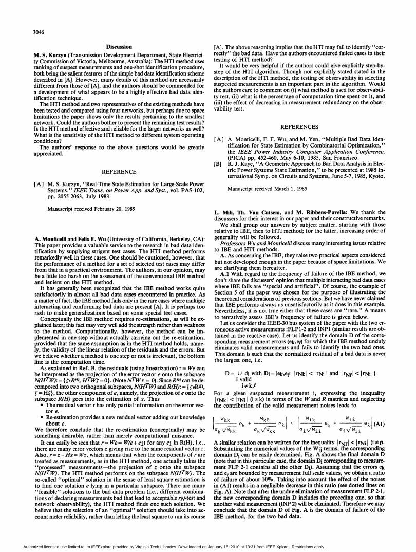
Let us consider the IEEE-30 bus system of the paper with the two er-roneous active measurements :FLP1-2 and INP1 (similar results are ob-tained in the reactive case). Let us identify the domain D of the corre-sponding measurement errors (ek,ee) for which the IBE method undulyeliminates valid measurements and fails to identify the two bad ones.This domain is such that the normalized residual of a bad data is neverthe largest one, i.e.

D= U di with Di=[ek,e(: IrNkI <lrNiI and IrNel <IrNilIi valid

i k,fFor a given suspected measurement i, expressing the inequalityrNk < I rNi (i * k) in terms of the Wand R matrices and neglecting

the contribution of the valid measurement noises leads to

II Wkk

ork VWkk

Wkk

0k \/Wkk

Wik< e

OFi,Wii

WitZ.oi.,/w ,(Al)

A similar relation can be written for the inequality rN I < IrNi (i * ).Substituting the numerical values of the Wij terms, the correspondingdomain Di can be easily determined. Fig. A shows the final domain D(note that in this particular case, the domain Di corresponding to measure-ment FLP 2-1 contains all the other Di). Assuming that the errors ekand ei are bounded by measurement full scale values, we obtain a ratioof failure of about 10%. Taking into account the effect of the noisesin (Al) results in a negligible decrease in this ratio (see dotted lines onFig. A). Note that after the undue elimination of measurement FLP 2-1,the new corresponding domain D includes the preceding one, so thatanother valid measurement (INP 2) will be elmiinated. Therefore we mayconclude that the domain D of Fig. A is the domain of failure of theIBE method, for the two bad data.


3047

Obviously, this development should be repeated for all the possiblelocations of two, three, . . . bad data in order to get an assessment ofthe overall behavior of IBE, for a given measurement configuration. Notethat the representative point of the example of Section 5.2 falls into thehachured area but admittedly this case is not isolated.

Fig. A. Domain D of failure of the IBE method

A.2. Concerning the one-step implementation of the measurementelimination: we agree with the discussers that computationally the elimina-tion of multiple measurements can be carried out in one step, by simplycorrecting the corresponding measured values (which allows keeping thesame factorized gain matrix in the subsequent re-estimations). Howeverthe main concern is to properly correct these measurements, i.e. correctthem in such a way that the correction will have exactly the same effectas a "pure" elimination.

As is mentioned in Section 4.1.3 of the paper, this requires:(i) computing the measurement correction by means of Eq. (9):

-(zs)cor = Zs - W- Issrswhere the off-diagonal terms of Wsscannot be neglected forinteracting measurements;

(i i) correcting correspondingly the W-matrix, in order to reflect the(fictitious) eliminations;

(iii) re-correcting the previously treated measurements when newmeasurements are to be corrected.

Practical experience has shown that corrections which do not fulfillthese three requirements may lead to meaningless results. This is illustratedin the two following examples.

Considering the IEEE system again, two bad data have been introducedas follows:

INP 29: h(x) =- 2.4 MW z = 100. MWINP 30: h(x) = -10.6 MW z = 50. MW

These two bad data are interacting but the value of the errors are suchthat the IBE method with "pure" elimination performs well. The listof suspected measurements obtained after estimation is given in columnI of Table A below.

In a first case, the measurements are treated through the approximatecorrection formula (8) of the paper, while keeping the Wii coefficientsalways constant. Measurement INP 29 is first corrected. This yields thesuspected measurements listed n column II. Since there remains only onebad data (INP 30), the latter should have the largest rNi I; however,because incorrect Wii coefficients have been used when computing thenew rNi, FLP 27-30 is the most suspected one and is unduly corrected.Due to erratic corrections, mine successive cycles have been required beforethe detection test becomes negative and INP 30 has never been correctedat all!

In a second case, we have tried to improve the above results by"refreshing" the W,i terms after each correction (according to require-ment (ii)); these coefficients are given in Table B below (note that Wiiis undefined for the corrected measurements). Column IV of Table Ashows that INP 30 is, as expected, at the top of the list. Although thetwo erroneous measurements have been corrected, the detection test re-mains positive (see column V).

These two examples illustrate that a proper correction of multiple baddata must obey the above three requirements. We are thus led to the

Table A: Successive Lists of Suspected Measurements with one-by-oneCorrection

Diag(W) non refreshed Diag(W) refreshed

COLUMN I: COLUMN II: COLUMN III : COLUMN IV: COLUMN V1st estimation 2nd estimation 3rd estimation 2nd estimation 3rd estimation

Measurts. rN Measurts. rM Measurts. rN Measurts. rN Measurts. rN

INP 29 118.95 FLP 27-30 25.22 INP 26 12.79 INP 30 28.28 FLP 27-30 26.30INP 30 108.46 INP 30 18.89 FLP 27-28 -9.18 FLP 27-30 25.22 FLP 27-29 -15.35FLP 29-27 - 45.10 FLP 27-29 -10.89 FLP 29-27 7.94 FLP 27-29 -12.39 FLP 29-27 14.41FLP 27-29 42.84 FLP 29-27 10.86 FLP 27-29 -7.75 FLP 29-27 11.71INP 26 34.22 INP 26 8.76 FLP 24-25 5.47 INP 26 9.47FLP 27-28 -26.07 FLP 27-28 -6.00 INP 30 5.10 FLP 27-28 -6.07FLP 27-30 21.63 FLP 24-25 3.81 FLP 28- 6 -4.22 FLP 24-25 3.82FLP 24-25 13.56 INQ 29 -3.21 INQ 29 -3.53 INQ 29 -3.22FLP 28- 6 -9.88 FLP 28- 6 -3.15 INQ 30 -3.36 FLP 28- 6 -3.16FLP 6-28 8.83 FLP 6-28 3.15FLQ 24-25 -6.09FLP 24-22 5.67INQ 26 -4.15FLP 28- 8 -3.95IVf 27 -3.87FLP 4-12 -3.64FLQ 4-12 -3.22FLP 6-9 -3.20FLP 12-15 -3.19

performed performed performedcorrection correction correction

INP 29: -42.69 MW FLP27-30 :- 14.9 MlW INP 30 : 23.20 MW

adequate correction adequate correction adequate correctionINP 29: -42.69 MW INP29 : -39.99 MW INP 29 : - 5.52 MW

FLP 27-30 :-20.87 MW INP 30 : - 10. 19 MW


3048

conclusion that the W- lss matrix - required in the HTI method - isanyway necessary to properly and efficiently face the problem of multi-ple bad data, whatever their interaction.

Table B: Diagonal Elements of W-Matrix

\ Wji INP 29initial INP 29 and

configuration eliminated INP 30Measurements eliminated

INP 29 0.445 -

INP 30 0.352 0.157 -

FLP 29-27 0.773 0.665 0.574FLP 27-29 0.814 0.629 0.557INP 26 0.354 0.303 0.260FLP 27-28 0.714 0.698 0.670FLP 27-30 0.840 0.840 0.262FLP 24-25 0.610 0.608 0.602FLP 28- 6 0.944 0.940 0.938INQ 29 0.469 0.465 0.469

B. The other points raised by Professors Wu and Monticelli concernthe very principle of the HTI method and are now successively discussed.

B.1 We fully agree that elimination-reestimation adds knowledge aboute: the HTI method also takes full advantage of this additional informa-tion. This follows from a property of the POE estimate, proved in Ref.[21]:

es = W-Issrs = Zs - hs(xc) (A2)where xc is the state estimate based on the remaining zt measurements,i.e. those remaining after eliminating the s selected ones.This property is precisely at the root of the equivalence between correc-tion and elimination (as was already observed by the authors of Ref.[11]). However, the discussers do not consider the counterpart of theelimination: eliminating valid measurements wastes useful information,decreases the power of the detection test, and increases the interactionof the remaining bad data. These drawbacks are inexistent in the HTImethod which performs on the initial configuration: Eq. (A2) shows thates is based on Zs as well as zt.

B.2. Considering projection properties is indeed worthwhile since itallows gaining good insight into the theoretical understanding of the WLSestimator, as has already been observed and used in Ref. [C] below.Within this context, we agree with the discussers that the residual vectorr belongs to N(HTR - 1), since

HR-TRlr=O (A3)Now, what probably has escaped the discussers' attention is that the vectorof concern in POE and hence in HTI is not r but a subvector rs of it,for which the above property is no longer valid. Indeed, partitioning (A3)according to selected and other measurements yields:

T -1 T -1HSRSr5+ H~Rt rt = 0

and Eq. (A4) must be considered instead of Eq. (A3).B.3. We agree with the discussers that the residual vector r contains

partial information on the error vector e: this is precisely why we do notrely on residuals but rather on error estimates which are "faithful pic-tures" of the errors. Another question evoked by the discussers is theexistence of multple error vectors leading to the same residual vector rs,i.e. there are many es,et satisfying the basic relation:

rs = Wsses + Wstet (Wss regular by construction)Among all the possible solutions, HTI definitely provides the OPTIMALone in the statistical sense, since the estimate Rs = W- 'ssrs is:(i) unbiased, provided that all erroneous measurements are selected, whichis ensured by adequate measurement selection (see Ref. [21]);(ii) minimum-variance (i.e. es is the most accurate estimate of es): thisimportant property is a recent result, shown and discussed in Ref. fD,E].

B.4. Referring to the terminology of Ref. [A] of the discussers, it isclear that the first selection of the HTI method provides a so-called "feasi-ble solution" which contains all the bad data; starting with this solu-tion, the successive refinements of the strategy fi lead to the smallest listof suspected measurements. The major differences with the method pro-posed in Ref. [A] are the following.

(i) In HTI, the convergence towards the final solution is guidedby the information contained in As (through the statistical test);HTI does not consider various "feasible solutions" as equiprob-able, but rather it follows an "optimal path".

(ii) The procedure is not combinatorial since each selection is a sub-set of the preceding one.

(iii) In HTI each decision is taken with an upper bounded f-risk(the risk of declaring valid a false measurement is thuscontrolled).

B.5. The concept of measurement reliability could indeed enhance theefficiency of bad data identification. It has not been considered here whilemodeling measurements, but it could certainly be included in the variousmethods compared in our paper. In the HTI method, the meter reliabilitycan be easily taken into account by selecting preferentially thesemeasurements and/or by adapting the threshold in the statistical test.In particular, one could consider as unreliable a measurement that hasbeen labeled false in a previous estimation but has not been eliminatedfrom the data base.

Ref. [21] is mainly devoted to the theoretical aspects of the HTI methodand offers a relatively wide spectrum of practical schemes. In the mean-time, intensive numerical testing as well as the implementation of HTIin the regional control center of the Belgian UNERG Companpy led usto establish appropriate practical schemes. These considerations and thecorresponding results will be the subject of a future publication; onlyessential aspects are discussed hereafter at the request of Professors Wuand Monticelli.

Fig. B presents the main steps of HTI, while Fig. C details the initialselection, a keypoint of the method. The other measurement selectionmentioned on Fig. B is similar to the latter and need not be detailed.The most salient feature of this procedure is the use of the well-known

matrix inversion lemma, for the computation of P55 = W- i.e.

with

-1 HTR-1 -1 T-1w-l (I- H =-I +H ZHJRSt= 5+ 5HS [Rs H ZHS] t ssI~ =XZ15[R-15H]'4

(A5)(A6)

These two formulae are used in a recursive way, each time a new measure-ment is added to the selection; in fact, in this case, Eq. (A6) reduces to:

wheren-s = t +n-s+I Ii lYkT-s+i

2 TD1 1a-hi nm-s+1 hi (scalar) (A7)

hi is the column vector or H relative to the i-th measurement.The advantages of this technique are manifold.

(i) It avoids a full inversion of WsS for each group of selectedmeasurements.

(ii) The computation of rss = W- Iss being rapid, the J(xc) -test(which requires es and hence rss) can be applied each time anew measurement is selected; this allows stopping the selectionas soon as all the bad data have been imbedded. Now, thesmaller the initial selection, the faster the identification.

(iii) The quantity Di in Eq. (A7) is used as a NUMERICAL observa-bility test. Indeed Di = 0 (in practice Di <eDb2i) means that thecorresponding measurement may not be included in the selec-tion (this measurement is in stand-by and will replace a measure-ment declared valid in a subsequent selection). Di being availableanyway, the observability test is thus a simple by-product ofthe error estimation. The corresponding computing time isnegligible and no special additional program is required.

Finally, let us observe that in the case of a single bad data, HTI isas fast as IBE. Indeed in such a situation:

- the erroneous measurement is selected first;- the J(2c) - test is directly negative;- the hypothesis test on esi is necessarily positive and no further refine-

ment is required;- the corresponding measured value is directly corrected.

Note also that a new detection test, after the state reestimation, is useless.


3049

Fig. B. The overall algorithmMake a (proper) initial selection

[measurements are classified into: selected)stand-by} (suspected)others (valid)

REPEAT:Apply the hypothesis test to each selected measurementIf the test is positive for some measurements:

THEN: make a new selection =measurements with positive test+ as many stand-by measurements as possible;

UNTIL the test is negative for all the selected measurements;[the latter are the bad data]

correct selected measurements : Zs = zs - esre-estimate the state (with fixed gain matrix).

Fig. C. The initial selections =0F. =EREPEAT:

Search for the (not yet selected) measurement withmaximum rNi ; let i be this measurement

compute Di = 2ihiT h

IF D; e u2 THEN : this measurement is in stand-by;ELSE : this measurement is selected

s = s+lSe = St + 1' (E'hi h )

rss Is fs sHSReS-=rS Srs- T 4..-

2UNTIL s= smax or Jc <Xm-n-sFOR each suspected, neither already selected nor already in

stand-by measurementIF this measurement had initially a Wii > EW

THEN : compute Di = - hTE'"hIF Di <eDoal

THEN : this measurement is also in stand--by

Dr. Kurzyn: We are pleased that he confirms our conclusions relativeto the performance of the various identification methods.

1. As concerning our choice of the IEEE-30 bus system for the presen-tation of simulation results, it has been guided by the fact that this systemis largely known. Otherwise, the comparative study presented in the paperis general and applies to any network, whatever its size. Because similarsimulation results have been found on the four quoted networks, theillustrative examples of the paper are representative of the behavior ofthe various identification methods in front of the three types of BD whichmay arise in practice.

2. The only difference existing between small and large networks con-cerns the computation time. As for the HTI method, the difficulty (par-ticularly for large systems) presented by the computation of Ws5 maybe cleared through efficient ways: (i) The submatrix of L involved inW5s may be calculated through an updating of the factors of G. Presently,this new approach is under testing. (ii) A straightforward method is nowavailable. It consists of multiplying the inverse factored form of G bythe appropriate columns of the identity matrix and of using the sparsevector technique (see Ref. [F]). As mentioned in the closure of this lat-ter paper, this technique speeds up dramatically the computation of theoff-diagonal terms of the inverse matrix. Let us mention that, whateverthe size of the network, a selection involving more than 30 measurementsis rare.

3. About the sensitivity of HTI method: experience has shown thatthe linear assumption is valid whatever the operating point of the systemand whatever the measurement weighting factors.

Finally, we would like to draw some general conclusions inspired bythe experience we gained during the implementation of HTI.

(i) In obvious single bad data cases, the HTI method reduces tothe conventional IBE method.

(ii) In the case of multiple (whatever interacting or not) bad datathe main part of the computing effort, i.e., computation ofW- lss matrix is required of both, IBE and HTI methods. Atthe expense of a very little additional effort, HTI guaranteesthe identification of all bad data, and only of them.

(iii) The HTI method is easy to program and to implement (we haveimplemented it on a PDP-1 1/70 computer which is in chargeof various tasks currently existing in the control center). Ofcourse, a prerequisite of its programming is its understanding;in other words, one cannot expect an inexperienced engineer(who, e.g., has seldom got involved with state estimation-relatedfunctions) to successfully program it.

(iv) The claim according to which one should not bother aboutspecial multiple interacting bad data cases, which are anywaylikely to be successfully handled by the system's operator is inour opinion arguable. Indeed, as long as the system is smalland the operator experienced, the need for fully automatic stateestimation, security and the like functions is hardly felt. Thedifficulties arise when complexity increases beyond humancapacities.

REFERENCES

[C] K. A. Clements, G. R. Krumpholz, P. W. Davis, "Power SystemState Estirriation Residual Analysis: An Algorithm Using NetworkTopology", IEEE Trans. on PAS, vol. PAS-100, no. 4, pp.1779-1787, April 1981.

[DI L. Mili, Th. Van Cutsem, M. Ribbens-Pavella, "Decision TheoryApplied to Bad Data Identification in Power System State Estima-tion", to be presented at the 7th IFAC Symp. on Identificationand System Parameter Estimation, Univ. of York, U.K., July 3-7,1985.

El L. Mili, "Algorithmes Fiables d'Identification des Fausses Don-nees par Tests d'Hypotheses", Internal Report (in French), Univ.of Liege, No. MBC/3, May 1984.

[F] W. F. Tinney, V. Brandwajn, S. M. Chan, "Sparse VectorMethods", IEEE Trans. on PAS, vol. PAS-104, no. 2, pp. 295-301,Feb. 1985.

Manuscript received March 26, 1985


Documents

capitat - Virginia Tech-Northern Virginia Center Data Identification Methods in... · IEEETransactions on PowerApparatus and Systems, Vol. PAS-104, No. 11, November 1985 BAD DATA