Capital Taxes with Real and Financial Frictions∗

Jason DeBacker †

April 2018

Abstract

This paper studies how frictions, both real and financial, interact with capital taxpolicy in a dynamic, general equilibrium model with heterogeneous firms. Comparativestatics show that tax policy can have substantially different effects depending uponthe frictions present. Analytical and numerical exercises show that accounting for firmheterogeneity is important when evaluating the responses of economic aggregates tocapital tax policy. The effects of tax cuts on allocational efficiency are found to bequantitatively significant, often accounting for the majority of the change in outputfollowing a reduction in taxes on capital.

JEL Classifications: D21; E22; G31; H25

Keywords: Corporate Finance; Firm Dynamics; Capital Taxation; Allocational Effi-ciency

Taxes on capital take many forms. Most common are the taxation of capital gains,

corporate profits, and dividend payments. The choice of tax instrument can affect corporate

investment policy and thus, if a government finds it optimal to tax capital, it must choose

among these tax instruments. Beyond taxes, investment behavior is also shaped by the real

and financial frictions firms face. In the following analysis, I study how real and financial

frictions interact with tax policy in an economy with heterogeneous firms. I use comparative

statics to understand how taxes affect investment decisions when firms face various frictions.

In addition, I decompose the changes in output following tax cuts to determine the effects

of tax policy on allocational efficiency.

This paper relates three well-established literatures. Firm dynamics have an extensive

literature in both economics and finance. Economists have largely focused on the role of real

∗I would like to thank Pablo D’Erasmo, Richard W. Evans, Russell Cooper and seminar participants atthe 2008 Midwest Macro Meetings, the University of Georgia, Georgia State University, and the Office ofTax Analysis for helpful comments.†Darla Moore School of Business, University of South Carolina, T: 803-777-1649, E: ja-

son.debacker@moore.sc.edu

1

frictions in explaining investment behavior (e.g., Cooper and Haltiwanger (2006)) whereas

those in finance have tended towards the use of financial frictions to explain the behavior of

firms (e.g., Hennessy and Whited (2005)). There has been strikingly little overlap between

these two lines of research.1 The typical finance paper takes financial frictions seriously,

but assumes the real frictions are quadratic in nature to support Q-theory based regres-

sions. Economists often ignore financial frictions, but allow for more flexible specifications

of the real costs of adjusting the firm’s capital stock. I span these two literatures, allowing

for non-convexities in real and financial frictions to affect firm dynamics. Distinguishing

between real and financial frictions is potentially important in the evaluation of tax pol-

icy. For example, with the quadratic costs of adjustment typically assumed in the finance

literature, firms’ investment is less elastic with respect to current cash flows, and thus tax

policy will be found to have relatively small effects on aggregate investment. The economics

literature citing the importance of non-convexities in capital accumulation decisions (e.g.,

Cooper and Haltiwanger (2006)), on the other hand, suggests cash flow can be very im-

portant in explaining investment behavior. Empirical tests of Q-theory such as Gilchrist

and Himmelberg (1995) support the significance of cash flow in explaining investment rates.

Miao (2008) shows that non-convexities in the costs of adjusting capital can lead to a larger

response of investment behavior to tax policy. Similarly, financial frictions can increase the

significance of cash flow because external financing is more expensive. Financial frictions

also drive a wedge between internal and external funding, which dampen the effects of tax

policy. Understanding these costs is key to understanding what drives the capital elasticity

of output and other determinants of the impact of tax policy (Chirinko (2002)).

The following study also relates to the public finance and macroeconomics literature on

the aggregate, general equilibrium effects of capital taxation (Auerbach and Kotlikoff (1987),

Barro (1989), Baxter and King (1993)). Important in the public finance literature are the

two main views of dividend taxation. The “traditional view” suggests the marginal source

of funds for investment is new equity and the return on investment is used to pay dividends.

In this view, dividend taxes influence the investment decisions of firms by affecting the value

1Notable exceptions include Cooley and Quadrini (2001), Cooper and Ejarque (2003) and Bayraktar,Sakellaris and Vermeulen (2005).

2

of the investment via the after tax value of dividend income. Alternatively, the “new view”

suggests firms use internal funds to finance investment and so do not issue new equity. This

means dividend taxes do not affect investment decisions since a dividend tax cut does not

affect the user cost of capital. Poterba and Summers (1985) analyze dividend taxation in

a dynamic model and find support for the traditional view. However, the empirical results

have been mixed, as Desai and Goolsbee (2004) find support for the new view. The model

in this paper nests both views. Depending on the firm’s capital stock and productivity, its

marginal source of funds may be internal or external funds.

I make two main contributions in this paper. First, I provide an analysis of tax policy

when firms face both convex and non-convex costs to adjusting capital and costly external

financing. Auerbach (1979b), Edwards and Keen (1984), and Poterba and Summers (1985)

are examples of papers analyzing capital taxes without frictions. Gourio and Miao (2010),

Gourio and Miao (2011), and House and Shapiro (2006) examine tax policy in models with

quadratic costs of capital adjustment. Although Gourio and Miao (2010) include a section

describing the effects of tax policy with marginal costs to issuing equity, they do not allow

for non-convexities in either the real or financial costs facing firms. Miao (2008) studies

the effects of fixed costs of capital adjustment on results of tax policy, but does not include

financial costs. I allow for non-convexities in both the real and financial costs. Given

the evidence of Hennessy and Whited (2007), Whited (2006), Cooper and Haltiwanger

(2006), and Gilchrist and Himmelberg (1995), non-convexities play an important role in

the investment and financing behavior of firms. The second significant contribution is the

decomposition of the effects of tax cuts into their allocational and incentive effects. The large

role for allocational efficiencies in the effects of tax policy on economic output underscore

the importance of modeling firm heterogeneity. Indeed, I find that changes in allocative

efficiency account for more than half of the change in output following a cut in the dividend

tax rate or corporate income tax rate.

The paper is organized as follows: Section 1 presents evidence on the investment behavior

of firms and their responses to tax policy. Section 2 describes the model. Section 3 discusses

the investment decisions of firms and how they are affected by frictions and taxes. I provide

numerical comparative statics for models with and without non-convexities in Section 4.

3

Section 5 concludes and discusses ideas for future research.

1 Investment Behavior and Evidence of Real and Financial

Frictions

1.1 Investment Facts

Costs of raising external funds and costs associated with changes in a firm’s capital stock

reflect many different factors which are difficult to measure directly or precisely (Cooper and

Haltiwanger (2006)).2 Because of this, these costs are typically studied indirectly, by looking

at investment behavior. Investment behavior at the plant and firm level is characterized

by:

1. An investment rate distribution that is non-normal and skewed to the right, with fat

tails and a mass around zero.

2. Long periods of inactivity punctuated by bursts of intensive investment.

3. A “low” correlation between investment rates and measures of marginal Q.

4. A “high” correlation between investment rates and measures of cash flow.

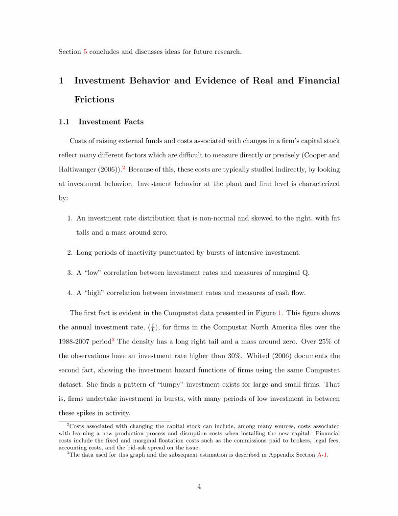
The first fact is evident in the Compustat data presented in Figure 1. This figure shows

the annual investment rate, ( ik ), for firms in the Compustat North America files over the

1988-2007 period3 The density has a long right tail and a mass around zero. Over 25% of

the observations have an investment rate higher than 30%. Whited (2006) documents the

second fact, showing the investment hazard functions of firms using the same Compustat

dataset. She finds a pattern of “lumpy” investment exists for large and small firms. That

is, firms undertake investment in bursts, with many periods of low investment in between

these spikes in activity.

2Costs associated with changing the capital stock can include, among many sources, costs associatedwith learning a new production process and disruption costs when installing the new capital. Financialcosts include the fixed and marginal floatation costs such as the commissions paid to brokers, legal fees,accounting costs, and the bid-ask spread on the issue.

3The data used for this graph and the subsequent estimation is described in Appendix Section A-1.

4

Facts 3 and 4 are evidenced in Gilchrist and Himmelberg (1995) and Fazzari, Hubbard

and Petersen (1988). Contrary to the predictions of Q-theory, both studies find a low

correlation between investment rates and measures of marginal Q using firm level data. In

addition, these studies find that investment is quite sensitive to measures of cash flow. As

in this paper, Gilchrist and Himmelberg (1995) use Compustat, while Fazzari et al. (1988)

use Value Line as their source for firm level data.

Facts 1-4 suggest either non-convexities in the real costs of adjustment or financial fric-

tions. Non-convex adjustment costs result in investment “bursts” as firms try to minimize

the fixed costs incurred when adjusting their capital stock by making fewer and larger in-

vestments. Cooper and Haltiwanger (2006) find behavior similar to 1 and 2 at the plant level

and estimate significant non-convexities in the costs of adjustment faced by plants. Non-

convexities in the costs of adjusting capital can also result in the lack of sensitivity of the

investment rate to measures of Tobin’s marginal Q that Fazzari et al. (1988) and Gilchrist

and Himmelberg (1995) report. An alternative explanation of the investment bursts and

sensitivity to cash flow is costly external financing (see, for example, Whited (2006) and

Fazzari et al. (1988)). For example, if issuing equity involves costs with economies of scale,

firms who finance projects with external funds will do so in bursts. Firms’ investment will

also be sensitive to the cash flows, as they try to finance with internal funds when possible.

This story is put forth by Gomes (2001) and Whited (2006).4 Altinkilic and Hansen (2000)

and Smith (1977) find the existence of such economies of scale in equity floatation costs.

0.0

05

.01

.015

Fra

ction

0 .5 1 1.5Investment Rate

Source: Compustat

Distribution of Investment Rates

Figure 1: PDF of Investment

4Although Cooper and Ejarque (2003) reject the hypothesis of financial frictions driving firm-level in-vestment dynamics, they do no attempt to match the financing behavior of firms.

5

1.2 Responses to Tax Changes

The Jobs and Growth Tax Relief Reconciliation Act of 2003 (JGTRRA) made two

major changes in law to promote capital formation and long run growth. First, the act

reduced the tax rate on capital gains for those in the top four income tax brackets (those

with federal marginal income tax rates of 25, 28, 33, and 35 percent) from 20% to 15%.

Second, the act brought the tax rate on dividends in-line with the rate on capital gains.

Previously, dividend income was taxed as regular income. The JGTRRA reduced the tax

rate on dividend income to 15% for those in the top four tax brackets, taxing dividends at

the same rate as capital gains. There is an abundance of work on the effects of the 2003 tax

cuts. Here, I offer some further evidence on the results of the policy change and its effects

on the financial and investment policies of firms. This helps to frame the discussion in the

following sections.

Chetty and Saez (2005) represents one of the most cited studies of the 2003 tax cuts.

The authors find a 20% increase in the amount of dividends distributed following the tax

cuts. More firms issue dividends and the amount of dividends issued increased. In Figure

2(a)-2(d), I present evidence on the effects of the tax cut on aggregate dividends, aggregate

new equity issuance, aggregate investment, and aggregate earnings. Figure 2(a) shows the

large increase in dividend distribution Chetty and Saez (2005) and others have documented.

Figures 2(b)-2(d) show increases in new equity issues, investment, and earnings following

the tax cuts of 2003.

Figures 3(a)-3(c) show the fractions of firms in various financing regimes before and

after the 2003 tax cuts. In the dividend distribution regime, the marginal source of funds is

retained earnings (this financing behavior corresponds to the new view of dividend taxation).

These firms are able to finance investment through retained earnings and are able to issue

dividends. In the equity issuance regime, the marginal source of funds is new equity (such

financing behavior corresponds to the traditional view of dividend taxation). These firms

issue new equity to finance investment. I classify firms in Compustat as being in the dividend

distribution regime if they are observed distributing dividends. Firms are classified as being

in the equity issuance regime if they issue new equity equal to at least 2% of the value of

6

.04

.045

.05

.055

.06

.065

.07

.075

.08

Ratio

1988 1990 1992 1994 1996 1998 2000 2002 2004 2006 2008Year

Source: Computstat

Dividend−Capital Ratio

(a) Dividend-Capital Ratio

.01

.02

.03

.04

.05

.06

Ratio

1988 1990 1992 1994 1996 1998 2000 2002 2004 2006 2008Year

Source: Computstat

Equity−Capital Ratio

(b) Equity Issuance - Capital Ratio

.15

.16

.17

.18

.19

.2R

atio

1988 1990 1992 1994 1996 1998 2000 2002 2004 2006 2008Year

Source: Computstat

Investment−Capital Ratio

(c) Investment - Capital Ratio

.25

.3.3

5.4

.45

.5R

atio

1988 1990 1992 1994 1996 1998 2000 2002 2004 2006 2008Year

Source: Computstat

Earnings−Capital Ratio

(d) Earnings - Capital Ratio

Figure 2: Aggregate Corporate Investment and Financing Behavior.

their capital stock.5 Firms who do not distribute dividends or issue new equity make up

the liquidity constrained regime. These firms finance investment through retained earnings.

They do not find it optimal to seek external funding to finance investment, but exhaust

their retained earnings and do not issue dividends.

As suggested by Figures 2(a) and 2(b), one can see an increase in the fraction of firms

who distribute dividends and in the fraction of firms who issue equity in Figures 3(a) and

3(b), respectively. In Figure 3(c), one can see the drop in the fraction of firms who are in

the liquidity constrained regime following the tax cuts. The movement of firms from this

regime accounts for much of the efficiency gains from the tax cuts of 2003.

5There exist a non-trivial number firms who both issue equity and distribute dividends. This behaviorconstitutes the “dividend puzzle”. The model presented in this paper can not account for this seeminglysuboptimal behavior. See Bernheim (1991) and Chetty and Saez (2007) for examples of papers attemptingto explain the puzzling behavior through models with asymmetric information. Auerbach (1979a) offersanother explanation using a overlapping generations model with population growth. Because my modelcannot account for the dividend puzzle, the firms who both distribute dividends and issue equity are classifiedas being in the dividend distribution regime.

7

.34

.36

.38

.4.4

2.4

4.4

6.4

8.5

Fra

ction o

f F

irm

s

1988 1990 1992 1994 1996 1998 2000 2002 2004 2006 2008Year

Source: Computstat

Dividend Distribution Regime

(a) Dividend Distribution Regime

.15

.2.2

5.3

.35

.4F

raction o

f F

irm

s

1988 1990 1992 1994 1996 1998 2000 2002 2004 2006 2008Year

Source: Computstat

Equity Issuance Regime

(b) Equity Issuance Regime

.22

.24

.26

.28

.3.3

2.3

4.3

6F

raction o

f F

irm

s

1988 1990 1992 1994 1996 1998 2000 2002 2004 2006 2008Year

Source: Computstat

Liquidity Constrained Regime

(c) Liquidity Constrained Regime

Figure 3: Financing Regimes.

2 Model

The model I use to analyze the effects of capital taxation incorporates the various

forms of capital taxes (capital gains, dividend income, corporate income) and accounts for

important general equilibrium effects of taxation. In addition, the model includes the real

and financial frictions firms face, which are necessary to explain the investment behavior

of firms. Finally, the model accounts for the observed financing decisions of firms where

one sees both internal and external sourcing of funding used for investment. That is, firms

behave according to both the new and traditional views of dividend taxation. My interest

is in the long-run effects of tax policy, thus I focus my analysis and model on the steady

state effects of an unanticipated change in tax policy.6 No aggregate uncertainty is present

in the model, but firms realize idiosyncratic productivity shocks. Below, I outline each part

of the economy. I begin with households.

6For an analysis of temporary changes in tax policy in a partial equilibrium model, see Gourio and Miao(2011). For a study of temporary and and predicted changes in tax policy, see House and Shapiro (2006).

8

2.1 Households

There is a representative household who supplies labor, trades shares in all firms and a

risk free bond, pays taxes, receives transfers, and consumes. Labor is supplied inelastically

and risk free bonds are in zero net supply. The household chooses consumption, equity

holdings, and bond holdings to solve:

max{Ct}∞t=0

∞∑t=0

βtU(Ct), (2.1)

where Ct is consumption in period t , β is the rate of time preference, and the utility

function has the standard properties (U ′ > 0, U ′′ < 0) and satisfies the Inada condition.

The household’s choice of C must satisfy:

Ct + bt+1 +

∫Vtθt+1dΓt =

∫[(1− τd)dt + V O

t − τg(V Ot − Vt−1)]θtdΓt

+ (1 + (1− τi)rt)bt + (1− τi)wtL+ Tt + Φt,

(2.2)

where bt+1 represents the holding of bonds expiring in period t + 1, Vt is the value of the

firm in period t, V Ot is the period t value of the shares outstanding in period t − 1, and

θt+1 are the shares of firms held in period t+1. The function Γt(kt, zt;wt) characterizes the

distribution of firms in period t and dt are dividends issued in period t. rt is the return on a

risk free bond and wt is the wage rate. The government transfers Tt to the household, and

τd, τg, and τi are the tax rates paid on dividend income, capital gains income, and labor

income, respectively. L is the amount of labor the household inelastically supplies to the

firms. The total financing costs paid by firms when raising external funding are returned

to the household and are represented by Φt.7

Equilibrium requires bt = 0 and θt = 1 for all t. Gomes (2001) shows that in a stationary

equilibrium the pricing kernel is given by β. That is, in a stationary equilibrium, r solves,

β(r(1− τi) + 1) = 1.

7Unlike the real costs of adjusting capital, the financial frictions are transaction costs paid by firms to fi-nancial intermediaries. To close the model, it is assumed that households own these financial institutions andthus receive these costs. The affect of this assumption is to increase household income and thus consumptionand investment by the household.

9

2.2 Firms

There are a continuum of ex-ante identical firms. Each firm chooses its capital stock,

hires labor, issues equity and distributes dividends to maximize firm value. Firms face

idiosyncratic shocks to productivity and thus, at any point in time, firms are heterogeneous

in both productivity and their capital stock.

If Vt is the value of a firm at time t, then the expected, after tax return to a shareholder

is given by:

Et(Rt) =(1− τd)dt + (1− τg)(EtV O

t+1 − Vt)Vt

(2.3)

V Ot+1 is the t+ 1 value of shares outstanding in period t and V O

t+1 = Vt+1 − st. Because the

only uncertainty derives from the idiosyncratic productivity shocks to the firms, there is

no aggregate uncertainty. Without aggregate uncertainty, asset pricing equilibrium implies:

Et(Rt) = 1 + (1 − τi)r, where r is the risk free interest rate. The right hand side of

this equation is the after-tax return on holding the risk free bond. That is, asset pricing

equilibrium requires the expected after-tax return on bonds and equity to be the same for

the household to trade both assets in equilibrium.

Using Equation 2.3 together with the asset pricing equilibrium condition, iterating for-

ward, and applying the transversality condition one can obtain the value of a firm at time

t:

Vt = Et

∞∑j=0

(1

1 + r(1− τi)/(1− τg)

)j (1− τd1− τg

dt+j − st+j)

(2.4)

Equation 2.4 is a standard representation of the value of a firm in the presence of taxes

(Auerbach (2002)). The equation says the value of the firm is the expected present value of

the after-tax dividends less the present value of new shares issued, which the current share

holders would have to purchase to maintain their claim on the same fraction of the firm’s

total dividends and profits.

From Equation 2.4, one can see the firm’s problem of maximizing shareholder value can

10

be represented by the following Bellman Equation:

V (k, z;w) = maxk′,d,s

(1− τd1− τg

)d− s+

1

1 + r(1− τi)/(1− τg)Ez′|zV (k′, z′;w′) (2.5)

In Equation 2.5, z denotes the firm’s productivity, k its capital stock, s its equity issuance.

Primed variable denote one period ahead values. Let υ(k, k′) characterize the costs a firm

faces when changing its capital stock and Φ(s) characterize the financial frictions the firm

faces when issuing equity. Additionally, let π(k, z;w) represent the firm’s profit function

given capital and productivity, δ be the rate of physical depreciation and τc be the taxes

paid on corporate income. The firm’s capital stock evolves according to the standard law

of motion for capital; k′ = (1 − δ)k + i, where i is the investment undertaken by the firm.

The firm faces the following constraints:

k′ − (1− δ)k + υ(k, k′) + d = (1− τc)π(k, z;w) + τcδk + s− Φ(s) (2.6)

d ≥ 0 (2.7)

s ≥ s¯

(2.8)

That is, it must be able to finance current investment and dividend distributions, dividends

must be non-negative, and equity issues must be above some lower bound. The first two

constraints are straight forward. The reasons for the bound on equity issues are de facto or

de jour restrictions on shares repurchases. There may be large costs associated with share

repurchases due to asymmetric information ( Brennan and Thakor (1990), Barclay and Jr.

(1988)) or there may be legal restrictions on share repurchases. For example, in the United

States, while share repurchases are allowed, regular repurchases may lead the IRS to treat

repurchases as dividends. Throughout, I assume s¯

= 0.8

8Admittedly, when s¯

= 0, as it does for the analysis this paper, one can not answer questions regardingthe observed “dividend puzzle”.

11

Firm’s combine capital and labor to produce output. The firm’s intratemporal profit

function is given by:

π(k, z;w) = maxl≥0{F (k, l, z)− wl} (2.9)

F (k, l, z) is the firm’s production function, which may be a decreasing returns to scale

function. The solution to this intratemporal problem yields the firm’s policy functions for

labor, l(k, z;w), and output, y(k, z;w). That is, the intratemporal labor demand decision

is determined by the capital stock and productivity of the firm and the market wage. Thus

I omit the choice of labor is from Equation 2.5.

The future value of the firm is discounted by a rate less than one if the household’s

rate of time preference parameter β is less than one. One can show the function V (k, z;w)

is concave, bounded, and continuous, so long as the firm’s production function F (k, l, z)

does not exhibit increasing returns to scale. Given this, one can apply the arguments of

Stokey, Lucas and Prescott (1989) to show the solution to Equation 2.5 exists and consists

of unique functions V (k, z;w), k′(k, z;w), d(k, z;w), and s(k, z;w).

2.3 Government

The government levies linear taxes on labor income, capital gains income, dividend

income, and corporate profits. The government does not issue debt. The revenues from

the taxes are assumed to be distributed in a lump sum manner to the household so the

government budget balances each period. The assumption of a lump sum transfer is made

for simplicity. Government spending on goods and services would introduce additional

distortions to the model unrelated to the effects of taxation on investment decisions, which

are the focus of the analysis. Additionally, government spending on goods and services

would mean tax cuts would necessarily have to be accompanied by spending reductions in

the stationary equilibrium, which would further complicate the analysis in a way that is

unnecessary to understand the mechanisms of interest.

The government budget constraint in any period (where I drop the time subscripts for

12

simplicity) is:

T = τc

∫(π(k, z;w)− δk)Γ(dk, dz;w) + τd

∫d(k, z;w)Γ(dk, dz;w)+

τiwL− τg∫s(k, z;w)Γ(dk, dz;w)

(2.10)

2.4 Stationary Distribution and Aggregates

Idiosyncratic shocks to the productivity of firms represent the only source of uncertainty

in the model. At each point in time the economy is characterized by a measure of firms,

Γt(k, z;w) for each level of capital stock k ∈ K = [k¯, k] and productivity, z ∈ Z = [z

¯, z]. For

there to be a stationary measure of firms, it must be the case that firms never accumulate

capital beyond some endogenously determined level k. If the optimal decision rule for

capital accumulation is increasing in z, it is clear the value of k is determined by the point

at which the decision rule k′(k, z;w) crosses the 45 ◦ line.

The law of motion of Γt(k, z;w) is given by:

Γt+1 = Ht(Γt) (2.11)

Let A and B be Borel sets of K and Z respectively and let P (z, z′) be the probability

the firm transitions from a productivity of z to productivity z′. The function Ht can then

be written as follows:

Γt+1(A×B) =

∫1{k′(k,z;w)∈A}P (z,B)Γt(dk, dz;w), (2.12)

where 1 is the indicator function.

I study the long run effects of tax policy and therefore focus the analysis on the invariant

distribution of firms denoted Γ∗. The invariant distribution is found by solving for the fixed

point in the mapping given by H. That is, Γ∗ solves Γ∗ = H(Γ∗). Stokey et al. (1989) state

the conditions necessary to prove the existence of an invariant distribution. The decision

rules of the firms and the stochastic process give rise to the mapping from the current

distribution of firms to the distribution of firms next period. Stokey et al. (1989) show

13

Γ∗ exists, is unique and the sequence of measures generated by the transition function,

{Hn(Γ0)}∞n=0, converges weakly to Γ∗ from any Γ0. The measure of firms is normalized to

one.

With the definition of the stationary distribution in hand, it is straight forward to

calculate the aggregate quantities in this economy:

• aggregate output

Y (Γ∗;w) =

∫y(k, z;w)Γ∗(dk, dz;w) (2.13)

• aggregate labor demand

Ld(Γ∗;w) =

∫l(k, z;w)Γ∗(dk, dz;w) (2.14)

• aggregate investment

I(Γ∗;w) =

∫(k′(k, z;w)− (1− δ)k)Γ∗(dk, dz;w) (2.15)

• aggregate adjustment costs

Υ(Γ∗;w) =

∫υ(k, k′(k, z;w))Γ∗(dk, dz;w) (2.16)

• aggregate financing costs

Φ(Γ∗;w) =

∫Φ(s(k, z;w))Γ∗(dk, dz;w) (2.17)

2.5 Stationary Equilibrium

Definition 1. (SRCE) A Stationary Recursive Competitive Equilibrium (SRCE) consists

of a wage rate w∗, a distribution of firms Γ∗(k, z;w∗), and functions V (k, z;w∗), l(k, z;w∗),

k′(k, z;w∗), d(k, z;w∗), and s(k, z;w∗) such that:

14

• Given w∗, V (k, z;w∗), l(k, z;w∗), k′(k, z;w∗), d(k, z;w∗), and s(k, z;w∗) solve the

firm’s problem.

• The stationary distribution is such that Γ∗(k, z;w∗) = H∗(Γ∗(k, z;w∗)

• Given w∗, the household maximizes utility subject to its budget constraint.

• The labor market clears: L =∫l(k, z;w∗)Γ∗(dk, dz;w∗)

• The goods market clears: Y (Γ∗;w∗) = C(Γ∗;w∗) + I(Γ∗;w∗) + Υ(Γ∗;w∗)9

The above are standard conditions for a stationary equilibrium. The value function and

policy functions are such that they solve the firm’s problem given prices. The evolution

of the distribution reproduces itself each period and is consistent with the equilibrium

decision rules of the firms and the distribution of idiosyncratic shocks to firms. Finally, the

representative household maximizes utility and markets clear.

Using a general equilibrium framework is important because the feedback of wages

dampens the effects of tax policy. For example, lowering dividend taxes increases the capital

stock and so increases the marginal product of labor and thus the wage. The higher wage

lowers employment and thus the marginal product of capital. Allowing wages to adjust

reduces the effect of tax policy on investment relative to a partial equilibrium model.

3 The Firm’s Decision Problem

Substitution of the budget constraint (Equation 2.6)) into the firm’s objective function

(Equation 2.5) leaves the firm with two decisions; the choice of capital stock and the choice

of equity issuance. When there are no non-convexities present, the first order conditions for

the choice of equity and the choice of capital, respectively, are:

s :

(1− τd1− τg

+ λd)(

1− ∂Φ

∂s

)+ λs = 1, (3.1)

9Note the absence of financial frictions in this condition. Financial frictions are not real costs. Thesetransactions costs are assumed to go to the households.

15

k′ :

(1− τd1− τg

+ λd)(

1 +∂υ(k, k′)

∂k′

)=

1

1 + r(1− τi)/(1− τg)Ez′|z

∂V (k′, z′)

∂k′, (3.2)

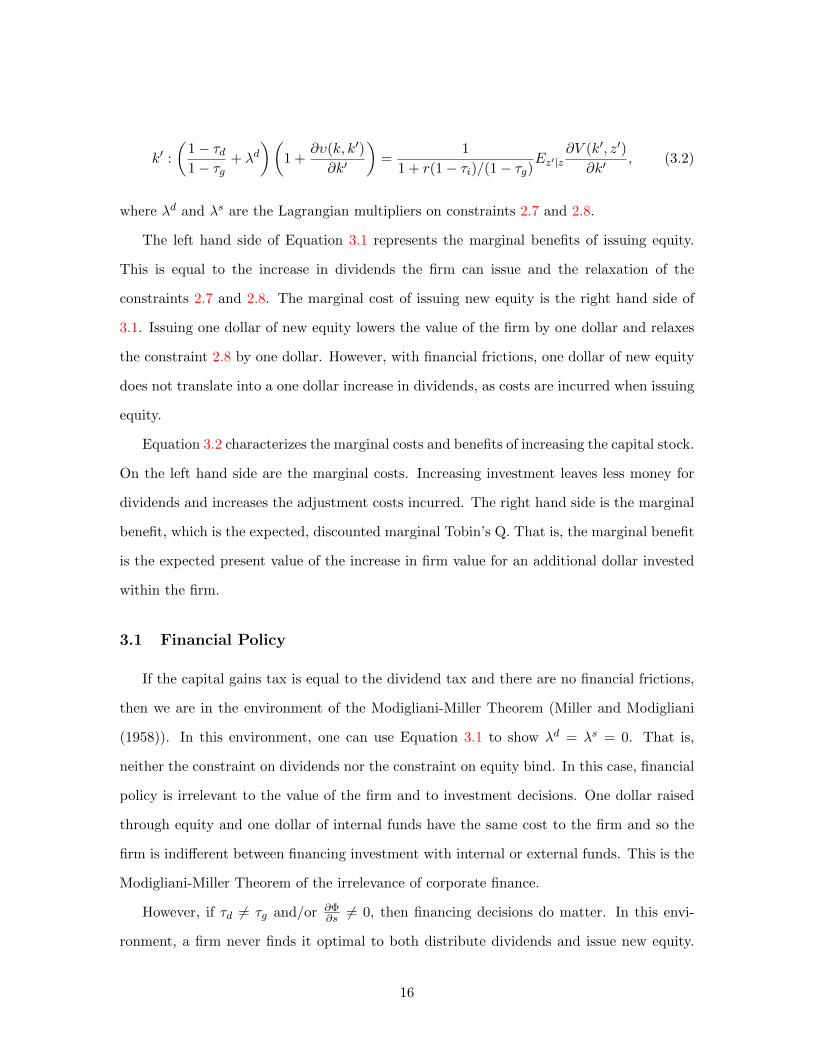
where λd and λs are the Lagrangian multipliers on constraints 2.7 and 2.8.

The left hand side of Equation 3.1 represents the marginal benefits of issuing equity.

This is equal to the increase in dividends the firm can issue and the relaxation of the

constraints 2.7 and 2.8. The marginal cost of issuing new equity is the right hand side of

3.1. Issuing one dollar of new equity lowers the value of the firm by one dollar and relaxes

the constraint 2.8 by one dollar. However, with financial frictions, one dollar of new equity

does not translate into a one dollar increase in dividends, as costs are incurred when issuing

equity.

Equation 3.2 characterizes the marginal costs and benefits of increasing the capital stock.

On the left hand side are the marginal costs. Increasing investment leaves less money for

dividends and increases the adjustment costs incurred. The right hand side is the marginal

benefit, which is the expected, discounted marginal Tobin’s Q. That is, the marginal benefit

is the expected present value of the increase in firm value for an additional dollar invested

within the firm.

3.1 Financial Policy

If the capital gains tax is equal to the dividend tax and there are no financial frictions,

then we are in the environment of the Modigliani-Miller Theorem (Miller and Modigliani

(1958)). In this environment, one can use Equation 3.1 to show λd = λs = 0. That is,

neither the constraint on dividends nor the constraint on equity bind. In this case, financial

policy is irrelevant to the value of the firm and to investment decisions. One dollar raised

through equity and one dollar of internal funds have the same cost to the firm and so the

firm is indifferent between financing investment with internal or external funds. This is the

Modigliani-Miller Theorem of the irrelevance of corporate finance.

However, if τd 6= τg and/or ∂Φ∂s 6= 0, then financing decisions do matter. In this envi-

ronment, a firm never finds it optimal to both distribute dividends and issue new equity.

16

Suppose τd > τg, as it was in the U.S. before the tax cuts of 2003. In this case, a firm will

be in one of three finance regimes.

Following Gourio and Miao (2010), call the the first regime type the equity issuance

regime. The marginal source of funds for firms in this regime is external equity. This

reflects the “traditional view” of dividend taxation. These firms do not issue dividends

and raise funds for investment by issuing equity. Firms in the equity issuance regime can

be thought of as “growth” firms. They have a high marginal product of capital, do not

distribute dividends and issue equity to finance their investments. Smaller firms, and those

with higher level of productivity, issue more equity. For firms in the equity issuance regime,

λd > 0 and λs = 0.

The second type of financing regime is the dividend distribution regime. Firms in this

regime finance investment internally, buy back shares to the extent possible, and issue divi-

dends with their remaining earnings. Those in the dividend distribution regime correspond

to the “new view” of dividend taxation. One can think of these firms as “value” firms.

Larger firms and those with lower productivity make up the firms in this regime. For firms

in the dividend distribution regime, λd = 0 and λs > 0.

The final regime type is the liquidity constrained regime. Constrained firms fund invest-

ment using internal funds, but do not distribute dividends. For these firms, the marginal

product of capital does not warrant raising funds externally, but is high enough that the

value of a dollar invested within the firm is higher than the value of a dollar invested outside

the firm. Hence no dividends are distributed and no equity is issued. In this regime, λd = 0

and λs = 0.

Figure 4 presents the regions (in the capital stock-productivity space) that constitute

the three financing regimes. In the top right are those firms with high levels of productivity

and/or a small capital stock. These firms have a high marginal product of capital and issue

equity. Firms in the bottom right of the area are those with a large capital stock and/or

low levels of productivity. These firms distribute dividends. As the tax wedge or finan-

cial frictions increase, the center region, representing firms who are liquidity constrained,

expands.

17

Capital

Productivity

s > 0

d > 0

s = 0,d = 0

Figure 4: Three Regimes

4 Numerical Comparative Statics

Here, I numerically evaluate the effects of tax policy when non-convexities are present.

I consider the responses to changes to the dividend tax, capital gains tax, and corporate

income tax, separately for four common specifications of investment frictions.

4.1 Model Specification

I assume the firms’ production functions are Cobb-Douglas; F (k, l, z) = zkαk lαl . Firms

may have decreasing or constant returns to scale. I also assume the productivity shocks

follow an AR(1) process; zi,t = ρzi,t−1 + ui,t, where ui,t ∼ N(0, σ).

I consider four models. In the first, there are no frictions. The second has convex costs

of adjusting capital and no financial frictions. The costs are assumed to be quadratic in

nature. Formally:

υ(kt, kt+1) =ψi2t2kt

(4.1)

This represents the most common specification in the literature on the effects of taxes on

investment (see, for example, House and Shapiro (2006)). The third model I consider has

non-convexities in the costs of adjustment represented by a fixed cost that is proportional

18

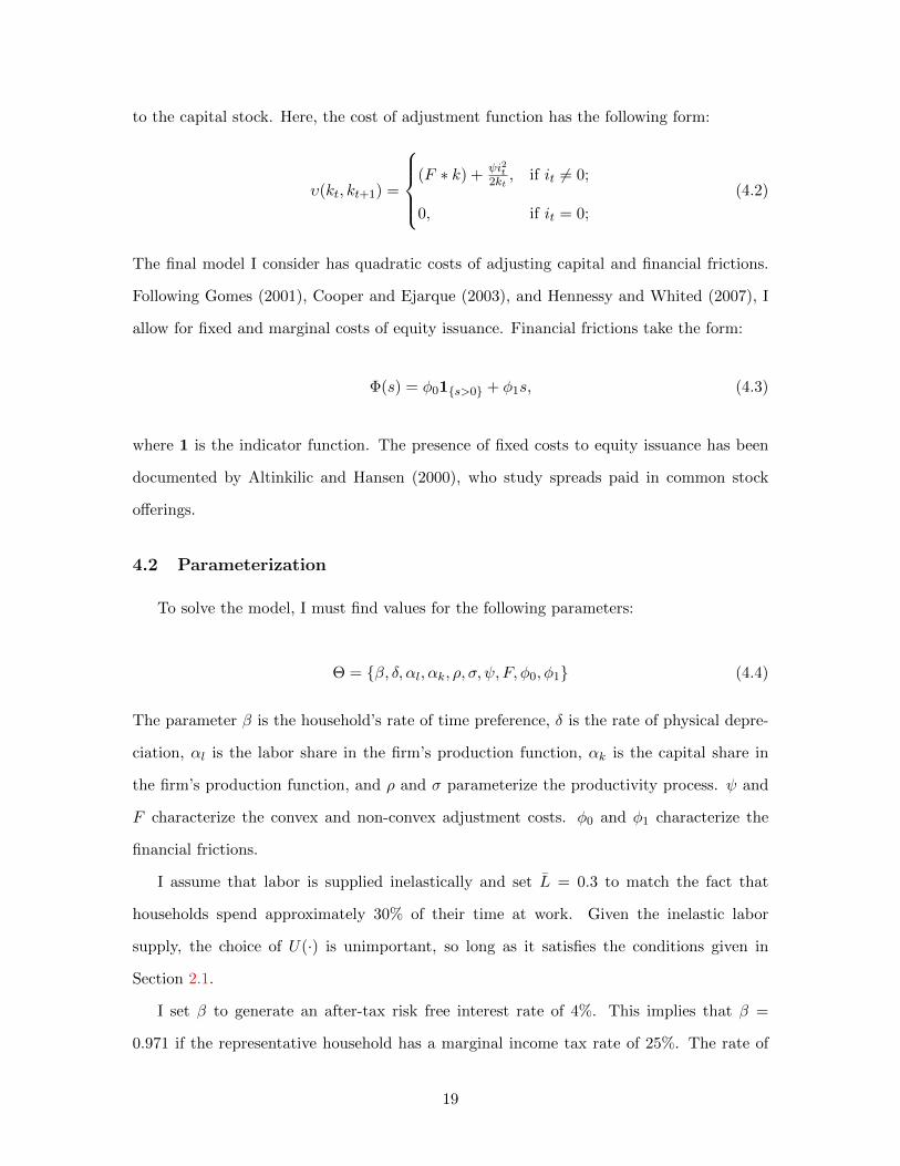
to the capital stock. Here, the cost of adjustment function has the following form:

υ(kt, kt+1) =

(F ∗ k) +

ψi2t2kt, if it 6= 0;

0, if it = 0;

(4.2)

The final model I consider has quadratic costs of adjusting capital and financial frictions.

Following Gomes (2001), Cooper and Ejarque (2003), and Hennessy and Whited (2007), I

allow for fixed and marginal costs of equity issuance. Financial frictions take the form:

Φ(s) = φ01{s>0} + φ1s, (4.3)

where 1 is the indicator function. The presence of fixed costs to equity issuance has been

documented by Altinkilic and Hansen (2000), who study spreads paid in common stock

offerings.

4.2 Parameterization

To solve the model, I must find values for the following parameters:

Θ = {β, δ, αl, αk, ρ, σ, ψ, F, φ0, φ1} (4.4)

The parameter β is the household’s rate of time preference, δ is the rate of physical depre-

ciation, αl is the labor share in the firm’s production function, αk is the capital share in

the firm’s production function, and ρ and σ parameterize the productivity process. ψ and

F characterize the convex and non-convex adjustment costs. φ0 and φ1 characterize the

financial frictions.

I assume that labor is supplied inelastically and set L = 0.3 to match the fact that

households spend approximately 30% of their time at work. Given the inelastic labor

supply, the choice of U(·) is unimportant, so long as it satisfies the conditions given in

Section 2.1.

I set β to generate an after-tax risk free interest rate of 4%. This implies that β =

0.971 if the representative household has a marginal income tax rate of 25%. The rate of

19

depreciation is set to generate the aggregate investment-capital ratio of 15.4% found in the

Compustat data.

Following the macro literature, I set αl = 0.65 because labor’s share of output is ap-

proximately 65% in the U.S. Given αl, I estimate αk, ρ, and σ as described in Appendix

Section A-2.

I set the parameters determining the sizes of these frictions to values found by others in

the literature who use similar models. I set ψ = 1.08 as done in Gourio and Miao (2010).

This value is similar to the parameter’s value in Cummins, Hassett and Hubbard (1994)

and elsewhere. To my knowledge, Bayraktar et al. (2005) provide the only estimate of non-

convex real costs of adjustment for firms in a model with financial frictions. While their

model allows for firms to also use debt and equity financing, I nonetheless set the fixed cost

of adjustment parameter to their estimate of F = 0.031.

External financing costs are set to φ0 = 0.04 and φ1 = 0.02. These values come from

Whited (2006) and Altinkilic and Hansen (2000).

The model parameterization is summarized in Table 1.

Table 1: Parameter Values Used in Numerical Comparative Statics

Parameter Value Source

β 0.971 r(1 − τi) = 0.04δ 0.154 I/Kαl 0.650 GM (2010)αk 0.297 Estimationρ 0.761 Estimationσ 0.213 Estimationψ 1.080 GM (2010)F 0.031 BSV (2005)φ0 0.040 Whited (2006)φ1 0.020 Whited (2006)

4.3 Responses of Aggregates to Tax Changes

For each model, I calculate the equilibrium values of the following aggregates: the

capital stock, output, the fraction of firms in each financing regime, wages, average Q, and

the tax multiplier. The baseline case is where taxes are at their pre-2003 levels for the

representative household who falls in the tax bracket with τi = 0.25 = τd and τg = 0.20. I

set τc = 0.34. From this baseline case, I make three changes to tax policy. First, I lower the

20

dividend tax rate four percentage points to 0.21. Next, I lower the capital gains tax rate

four percentage points to 0.16. The last policy change is to lower the corporate income tax

rate four percentage points to 0.30. For each model, I calculate the percent changes in the

aggregates and the tax multiplier of the respective tax change. I use four percentage point

changes for a two main reasons. First, they are close in size to the change in the long-term

capital gains tax rates resulting from JGTRRA of 2003, which cut the capital gains tax rate

from 20% to 15%. Furthermore, the Obama Administration has proposed increasing both

the capital gains and dividend tax rates five percentage points. Second, four percentage

points keeps a tax wedge even in the case of a reduction in the dividend tax rate for the

median household from it’s pre-2003 level of 25%. This means that the changes represent a

reduction in the tax wedge and not it’s elimination. If the tax wedge were eliminated, one

could not identify a firm’s financial policy in the cases without financial frictions since, as

the Modigliani-Miller Theorem (Miller and Modigliani (1958)) predicts, financial policy is

irrelevant in the absence of a tax wedge and financial frictions.

Table 2: Four Percent Cut in the Dividend Tax Rate

Aggregate No Cost ψ = 1.08 ψ = 1.08, F = 0.031 ψ = 1.08,(% Changes) φ0 = 0.04, φ1 = 0.02

QuantitiesCapital 22.96 0.57 1.87 -0.24Output 6.69 0.72 0.93 0.39

Financial PoliciesEquity Issuance Regime 0.00 19.25 5.18 9.20Dividend Distribution Regime 5.37 13.32 4.75 7.23Liquidity Constrained Regime -40.60 -34.18 -53.99 -2.21

PricesWage 5.51 0.70 0.89 0.41Average Q 23.39 6.25 2.70 3.41

Tax Multiplier(−∆G

∆T

)6.00 2.36 3.13 1.40

The model without frictions is the most responsive to changes in the dividend tax rate.

The no cost model is followed by the model with non-convexities, the convex model without

financial frictions, and, lastly, the model with financial frictions. A decrease in the dividend

tax rate can have both positive and negative effects on investment. On the one hand, a

dividend tax cut (when the tax rate on dividends exceeds the tax rate on capital gains)

results in a smaller tax wedge and a more efficient allocation of resources. As seen in three

of the four models, the capital stock is at least as large under the the dividend tax cut

21

because this effect dominates. On the other hand, a lower dividend tax rate will increase

the opportunity cost of investment for firms transitioning between the equity issuance and

dividend distribution regimes. This will have the effect of reducing those firms’ investment

in capital. This second effect is more apparent in models with financial frictions, where it

is more likely that relatively productive firms will distribute dividends because they face

large costs to accessing external financing. In the model with convex real costs and financial

frictions, the second effect swamps the first effect when dividend taxes are cut by 4% and

overall investment falls. However, even in this, case output does not fall because the tax

cut results in a better allocation of capital across firms. One can see this from the decrease

in the fraction of firms in the liquidity constrained regime. Among the models exhibiting

investment frictions, the model with non-convex costs to adjusting capital shows the largest

response to the dividend tax cut. The intuition for the result is that, due to the fixed costs

of investment, tax policy operates on both the extensive and intensive margins. More firms

invest, and those investing invest more. The large drop in the fraction of firms who are

liquidity constrained is evidence of these effects.

Table 3: Four Percent Cut in the Capital Gains Tax Rate

Aggregate No Cost ψ = 1.08 ψ = 1.08, F = 0.031 ψ = 1.08,(% Changes) φ0 = 0.04, φ1 = 0.02

QuantitiesCapital -1.81 3.27 2.05 2.96Output -1.79 0.57 0.33 0.47

Financial PoliciesEquity Issuance Regime -27.52 -15.07 -5.32 -15.67Dividend Distribution Regime -8.37 -13.69 -5.12 -15.13Liquidity Constrained Regime 92.67 30.97 57.08 4.45

PricesWage -1.60 0.54 0.36 0.55Average Q -3.42 -1.69 1.75 1.24

Tax Multiplier(−∆G

∆T

)-5.50 2.14 1.41 5.31

When the capital gains tax is lowered, there are two opposing effects on investment, and

thus the aggregate capital stock, in the stationary equilibrium. Investment may increase

because the tax change results in a higher after-tax value of the firm. However, a decrease

in the capital gains tax rate (from a rate less than the tax rate on dividends) increases the

wedge between internal and external funding and leads to a lower capital stock because

of a misallocation of resources to lower productivity firms. More firms are in the liquidity

22

constrained regime, ceteris paribus, after lowering the capital gains tax rate. These dual

effects are very evident in the first row of Table 3. In the model without frictions, the second

effect dominates, the fraction of firms in the liquidity constrained regime increases by over

92% and the aggregate capital stock falls. In models where the real costs of adjusting capital

are quadratic in nature, the first effect dominates and investment increases more than in

the other specifications. In general, the aggregates are most responsive in a model with no

frictions where firms’ investments are very elastic. Notably, the change in the fraction of

firms in the liquidity constrained regime is least responsive (measured by the percentage

change) in the presence of financial frictions. There is smaller percentage increase of firms in

the liquidity constrained regime in the presence of financial frictions because these frictions

increase the wedge between internal and external funding. Thus there are more constrained

firms in the baseline tax regime under this specification. The relative effect of a change in

taxes is thus smaller.

Table 4: Four Percent Cut in the Corporate Income Tax Rate

Aggregate No Cost ψ = 1.08 ψ = 1.08, F = 0.031 ψ = 1.08,(% Changes) φ0 = 0.04, φ1 = 0.02

QuantitiesCapital 2.42 3.05 3.73 2.29Output 0.28 1.17 1.27 1.06

Financial PoliciesEquity Issuance Regime 0.00 1.77 -0.39 6.56Dividend Distribution Regime 0.00 -4.48 0.71 -4.72Liquidity Constrained Regime -0.03 4.23 -3.14 0.81

PricesWage 0.86 1.13 1.28 1.08Average Q 6.34 4.49 3.57 4.51

Tax Multiplier(−∆G

∆T

)0.47 2.50 2.41 2.46

As noted in the previous section, a cut in the the corporate income tax rate always

results in an increase in investment. The numerical comparative statics for each model

bear this out. The capital stock increases most after the tax cut in the model without

frictions. As was the case with the dividend tax cut, the model with quadratic and fixed

costs of adjustment has the next largest response to the tax cut. Lower corporate income

taxes increase the firm’s after-tax cash flow. The presence of fixed costs to adjusting capital

results in firm investment decisions being particularly sensitive to cash flow and hence to

reductions in the corporate income tax. This is especially true when a tax wedge exists and

23

firms are more likely to fund investment with retained earnings.

Tax policy has differential effects depending upon the real and financial frictions present.

Magnitudes and directions of the changes in aggregates vary across models and tax instru-

ments. For example, the long run tax multiplier (the increase in output per dollar of tax

revenue foregone) for a corporate income tax cut vary between 0.47 and 2.50. Such differ-

ences highlight the importance of understanding the real and financial frictions firms face

when evaluating fiscal policy. Non-convexities generally result in investment being more

responsive to tax policy. The result is similar to those of Caballero, Engel and Haltiwanger

(1995), Cooper, Haltiwanger and Power (1999), and Caballero and Engel (1999) who find

that models with non-convexities in capital adjustment costs generate relatively large re-

sponses to aggregate shocks.

4.4 Allocational Efficiency

Changes in capital taxation affect investment in two ways. First, lower tax rates have

the effect of increasing the after-tax value of a firm. A higher marginal Q implies that a

given firm will invest more after the tax cut, all else equal. Call this the incentive effect

of taxation. Second, lower tax rates affect distribution of firms investing. For example,

lowering the dividend tax rate (when it is higher than the tax rate on capital gains) has the

effect of reducing the number of firms in the liquidity constrained regime by reducing the tax

wedge between internal and external financing. The result is that more high productivity

firms access external funding to finance investment. Call the effect of taxation on the

distribution of the capital stock across firms the reallocation effect.

Two indicators of allocational efficiency are total factor productivity (TFP) and the

correlation between capital and productivity across firms. Let TFP be defined as TFP =

YKαkLαl . Table 5 presents the percentage change in TFP and the correlation between capital

and productivity by model and tax regime. The baseline case is that in which taxes are

at there pre-2003 levels (i.e., τi = 0.25, τd = 0.25, τg = 0.20, and τc = 0.34). The other

three columns represent a reduction in each of the taxes from the baseline. Looking across

models, we see that models with frictions have a much lower correlation between capital and

productivity than a model without frictions. Costs to adjusting capital or to accessing ex-

24

ternal financing discourage firms from adjusting their capital stock to the extent they would

in a frictionless environment. In all models with frictions, a dividend tax cut increases the

measures of allocational efficiency and a capital gains tax cut reduces allocation efficiency.

This is expected given the effects these policies have on the tax wedge and the number of

firms in the liquidity constrained regime (see Tables 2 and 3). The effect of the dividend

tax cut on TFP is counter intuitive in the frictionless model. TFP falls after a dividend

tax cut (and reduction in the tax wedge) in this specification. What drives the result is the

disproportionate increase in the capital stock among firms with lower productivity. As seen

in Table 2, the dividend tax cut results in an almost 23% increase in the capital stock, but

only a 6.7% increase in output. Because of the absence of investment frictions, fewer firms

are liquidity constrained. The reduction in the tax wedge has the largest percentage impact

on those who were constrained prior to the tax cut, but not constrained following the tax

cut. These are more likely to be firms with lower productivity. The model with fixed costs

to adjusting capital show smaller changes in allocative efficiency than the model with only

quadratic costs of adjustment. Although Tables 2-4 show that the model with fixed costs

to generally be more responsive to tax changes, the effects on allocative efficiency aren’t

are large (as compared to the other specifications). This has to do with the distribution

of capital across firms of varying productivity prior to the tax change. In the model with

fixed costs, investment is done by the most productive firms. Thus, as the dividend tax

cut reduces the tax wedge, the effect on the distribution of capital across firms is smaller

relative to other models where capital effectively distributed prior to the tax cut.

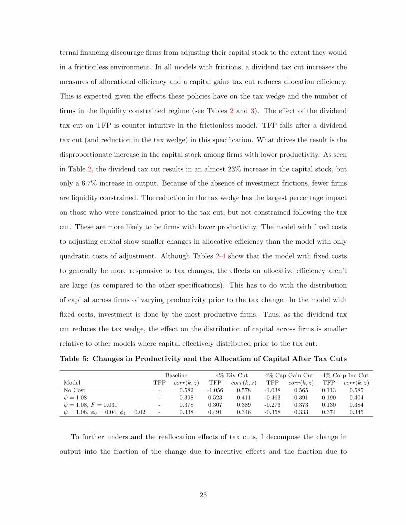
Table 5: Changes in Productivity and the Allocation of Capital After Tax Cuts

Baseline 4% Div Cut 4% Cap Gain Cut 4% Corp Inc CutModel TFP corr(k, z) TFP corr(k, z) TFP corr(k, z) TFP corr(k, z)

No Cost - 0.582 -1.056 0.578 -1.038 0.565 0.113 0.585ψ = 1.08 - 0.398 0.523 0.411 -0.463 0.391 0.190 0.404ψ = 1.08, F = 0.031 - 0.378 0.307 0.389 -0.273 0.373 0.130 0.384ψ = 1.08, φ0 = 0.04, φ1 = 0.02 - 0.338 0.491 0.346 -0.358 0.333 0.374 0.345

To further understand the reallocation effects of tax cuts, I decompose the change in

output into the fraction of the change due to incentive effects and the fraction due to

25

allocation effects. Output in the model economy can be written as:

Y =

∫zkαk lαlΓ(dk, dz;w)

=

∫zkαk l(k, z;w)αlΓ(dk, dz;w)

=(αlw

) αl1−αl

EΓz1

1−αl + EΓkαk

1−αl + covΓ

(z

11−αl , k

αk1−αl

)︸ ︷︷ ︸Allocation Component

,(4.5)

where EΓ denotes the expected value given the distribution of firms defined by Γ(k, z;w)

and covΓ(·, ·) is the covariance across this distribution. The fraction of Y accounted for by

the allocational component is represented by the covariance term. Letting Ybase be output

under the baseline tax system and Ycut represent output under a decrease in one of the tax

rates, the percentage change in Y due to the reallocation of capital from lower to higher

productivity firms is:

%∆Y due to reallocation =

(αlwcut

) αl1−αl covΓcut

(z

11−αl , k

αk1−αl

)−(

αlwbase

) αl1−αl covΓbase

(z

11−αl , k

αk1−αl

)Ycut − Ybase

(4.6)

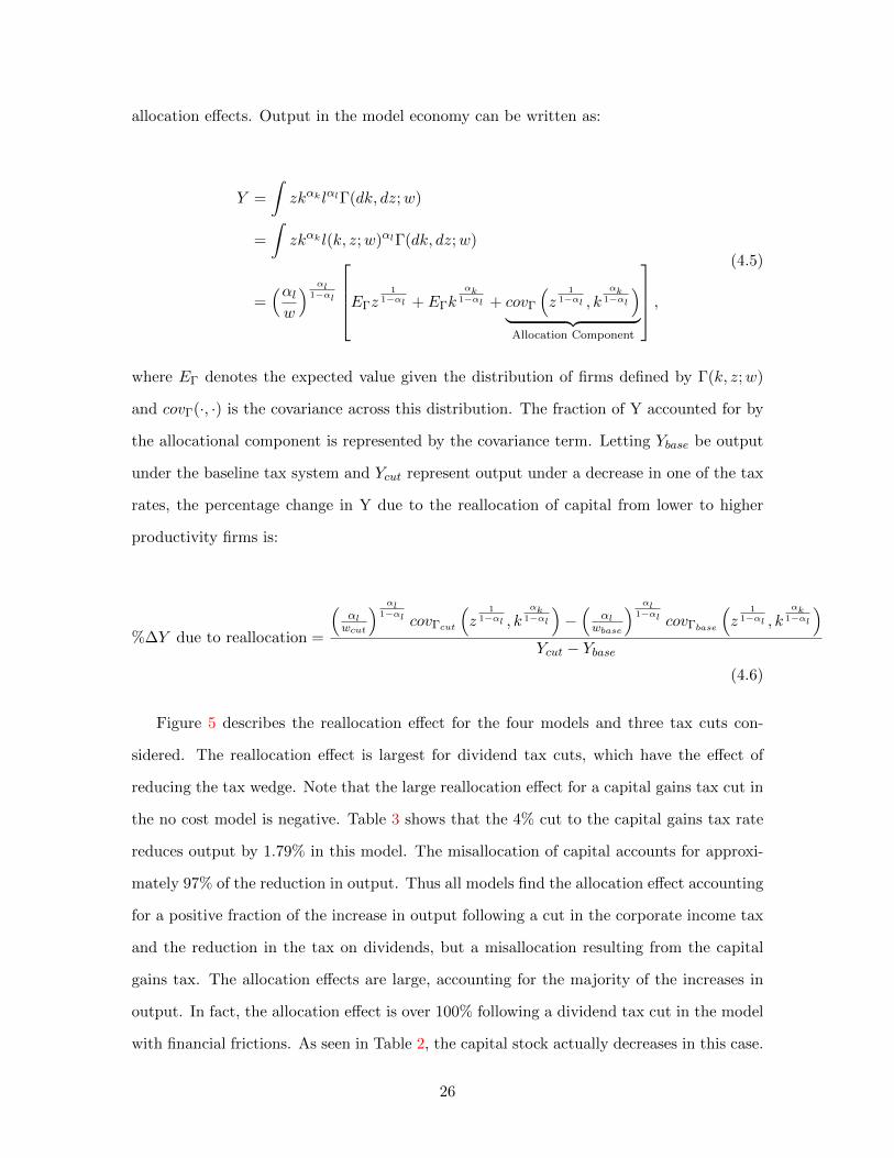
Figure 5 describes the reallocation effect for the four models and three tax cuts con-

sidered. The reallocation effect is largest for dividend tax cuts, which have the effect of

reducing the tax wedge. Note that the large reallocation effect for a capital gains tax cut in

the no cost model is negative. Table 3 shows that the 4% cut to the capital gains tax rate

reduces output by 1.79% in this model. The misallocation of capital accounts for approxi-

mately 97% of the reduction in output. Thus all models find the allocation effect accounting

for a positive fraction of the increase in output following a cut in the corporate income tax

and the reduction in the tax on dividends, but a misallocation resulting from the capital

gains tax. The allocation effects are large, accounting for the majority of the increases in

output. In fact, the allocation effect is over 100% following a dividend tax cut in the model

with financial frictions. As seen in Table 2, the capital stock actually decreases in this case.

26

However, the positive allocation effect overwhelms the reduction in investment; the more

efficient distribution of capital results in an increase in output.

4% Div Cut 4% Cap Gain Cut 4% Corp Inc Cut−0.4

−0.2

0

0.2

0.4

0.6

0.8

1

1.2Allocational Efficiency Effects of Tax Cuts

Tax Change

Fra

ctio

n o

f C

ha

ng

e in

Y D

ue

to

Re

allo

ca

tio

n

No Cost Model

psi=1.08

psi=1.08, F=0.031

psi=1.08, phi0=0.04, phi

1=0.02

Figure 5: Reallocation Effects of Tax Cuts

Reallocation effects are largest when financial frictions are present. In such an environ-

ment, the fraction of firms in the liquidity constrained regime is greatest. A change in tax

rates may move many such firms to other financing regimes, aiding allocations efficiency.

This is especially true in the case of the dividend tax cut, which directly affects the size of

the tax wedge between internal and external financing. But it is also true of tax cuts that

affect the cash flows of these constrained firms, such as the cut to the corporate income tax.

Non-convex costs to adjusting capital make firms’ investment decisions relatively sensi-

tive to cash flows and thus models with fixed costs to adjusting capital show relatively large

responses of investment to tax cuts. However, these fixes costs are barriers to the reallo-

cation of capital across firms. Thus the model with quadratic and fixed costs to adjusting

physical capital, in which firms face the largest costs to adjusting capital, is the model

where the reallocation effects are smallest. The reallocation effects are still significant in

spite of these adjustment costs, accounting for over 60% of the increase in output following

a dividend tax cut and over 50% following a cut in the corporate income tax.

27

5 Conclusion

The analysis in the preceding sections investigates the extent to which the aggregate

effects of tax policy depend on real and financial frictions in a general equilibrium model

with heterogeneous firms. Understanding how tax policy affects the investment decisions

of firms is important. The government, should it decide to tax capital, has several policy

tools from which to choose. The choice of tax instrument needs to be considered in light

of the economic impact it will have. I determine how frictions interact with three of these

instruments: taxes on dividend income, taxes on capital gains, and taxes on corporate

income.

In short, this paper shows frictions, both real and financial, matter when evaluating tax

policy. Relative to models with only convex costs of adjusting capital, models with non-

convexities in the costs of adjustment are often more responsive to tax policy. The presence

of financial frictions, on the other hand, dampens the response of aggregate investment

to changes in capital taxation. To put in perspective the importance of accounting for

investment frictions when evaluating tax policy, consider the predicted effects on output and

investment following from a permanent extension of JGTRRA. The model with quadratic

and fixed adjustment costs (as parameterized in Section 4.2) predicts a percentage change

in output 16.6% larger (1.8% vs. 1.5%) than that from a model with only quadratic costs

of adjusting capital. The model with non-convexities predicts a percentage increase in the

capital stock that is 46.6% larger (4.7% vs. 3.2%) than the model with only quadratic costs

of adjustment. The quadratic specification prevails among models with which tax policy is

evaluated (e.g., A Dynamic Analysis of Permanent Extension of the President’s Tax Relief

(2006), Gourio and Miao (2010)), but such models do not account for the sensitivity of

investment to capital taxation. Understanding this relationship is importance as policy-

makers wrestle with the question of whether or not to further extend the Bush tax cuts.

In addition, this paper highlights the importance of firm heterogeneity in the analysis of

the effects of tax policy. When changing marginal capital tax rates, allocational efficiencies

account for much of the resulting impact on output. In the case of a cut in the dividend

tax rate, these allocational effects are responsible for over 60% of the increases in output

28

across models with a wide range of investment frictions. These allocational effects can

be negative when the tax wedge between internal and external financing is widened. For

example, lowering the capital gains tax rate further below the tax rate on dividends may

not be efficiency enhancing because such a policy increases the tax wedge and results in a

(further) misallocation of capital.

Within the context of long run effects of unanticipated changes in tax policy, a number

of meaningful extensions to the model and analysis present themselves. Elastic labor supply

and heterogeneous households would strengthen any welfare analysis done with the current

model. Another extension is to allow firms to borrow and lend. Debt financing is important

for many firms, and with the tax advantages of debt, a source of interesting public finance

questions.

The work in this paper suggests several other questions for future research. Contrary

to the model presented here, changes in tax policy are often predictable and temporary.

Frictions are particularly salient in determining the outcome of anticipated changes in tax

policy. Convex and non-convex frictions are likely to result in large differences in the effects

of changes in tax policy when firms see the change approaching. Second, although the

presence of taxes may be one of the few certainties in life, almost as certain is change in tax

policy. That is, taxes may be permanent, but the specifics of taxation are not. The expected

duration of tax policy interacts with frictions as firms postpone or expedite their investment

decisions to engage in tax arbitrage. The effects of temporary tax policies greatly depend

on real and financial frictions.

References

A Dynamic Analysis of Permanent Extension of the President’s Tax Relief,Technical Report, Office of Tax Analysis, United States Department of the TreasuryJuly 2006.

Altinkilic, Oya and Robert S. Hansen, “Are There Economies of Scale in UnderwritingFees? Evidence of Rising External Financing Costs,” The Review of Financial Studies,Spring 2000, 13 (1), 191–218.

Auerbach, Alan J., “Share Valuation and Corporate Equity Policy,” Journal of PublicEconomics, June 1979, 11 (3), 291–305.

29

, “Wealth Maximization and the Cost of Capital,” Quarterly Journal of Economics,August 1979, 93 (3), 433–446.

, “Taxation and Corporate Financial Policy,” in Alan J. Auerbach and Martin Feld-stein, eds., Handbook of Public Economics, Vol. 3, Amsterdam: North Holland, 2002.

and Laurence J. Kotlikoff, Dynamic Fiscal Policy, Cambridge, UK: CambridgeUniversity Press, 1987.

Barclay, Michael J. and Clifford W. Smith Jr., “Corporate Payout Policy: Cash Div-idends Versus Open Market Repurchases,” Journal of Financial Economics, October1988, 22 (1), 61–82.

Barro, Robert J., “The Neoclassical Approach to Fiscal Policy,” in Robert J. Barro, ed.,Modern Business Cycle Theory, Harvard University Press, 1989, pp. 178–235.

Baxter, Marianne and Robert G. King, “Fiscal Policy in General Equilibrium,” Amer-ican Economic Review, June 1993, 83 (3), 315–334.

Bayraktar, Nihal, Plutarchos Sakellaris, and Philip Vermeulen, “Real Versus Fi-nancial Frictions to Capital Investment,” European Central Bank Working Paper, 2005.

Bernheim, B. Douglas, “Tax Policy and the Dividend Puzzle,” The RAND Journal ofEconomics, Winter 1991, 22 (4), 455–476.

Brennan, Michael J. and Anjan V. Thakor, “Shareholder Preferences and DividendPolicy,” Journal of Finance, September 1990, 45 (4), 993–1018.

Caballero, Ricardo J. and Eduardo M. R. A. Engel, “Explaining Investment Dy-namics in U.S. Manufacturing: A Generalized (S,s) Approach,” Econometrica, 1999,67 (4), 783–826.

, , and John C. Haltiwanger, “Plant-Level Adjustment and Aggregate Invest-ment Dynamics,” Brookings Papers on Economic Activity, 1995, 26 (2), 1–54.

Chetty, Raj and Emmanuel Saez, “Dividend Taxes and Corporate Behavior: EvidenceFrom the 2003 Dividend Tax Cut,” The Quarterly Journal of Economics, August 2005,120 (3), 791–833.

and , “An Agency Theory of Dividend Taxation,” NBER Working Paper 13538,October 2007.

Chirinko, Robert S., “Corporate Taxation, Capital Formation, and the SubstitutionElasticity between Labor and Capital,” National Tax Journal, June 2002, 55 (2), 339–355.

Cooley, Thomas F. and Vincenzo Quadrini, “Financial Markets and Firm Dynamics,”American Economic Review, December 2001, 91 (5), 1286–1310.

Cooper, Russell, John Haltiwanger, and Laura Power, “Machine Replacement andthe Business Cycle: Lumps and Bumps,” American Economic Review, September 1999,89 (4), 921–946.

30

Cooper, Russell W. and Joao Ejarque, “Financial frictions and investment: requiemin Q,” Review of Economic Dynamics, October 2003, 6 (4), 710–728.

and John C. Haltiwanger, “On the Nature of Capital Adjustment Costs,” Reviewof Economic Studies, July 2006, 73 (3), 611–633.

Cummins, Jason G., Kevin A. Hassett, and R. Glenn Hubbard, “A Reconsidera-tion of Investment Behavior Using Tax Reforms as Natural Experiments,” BrookingsPapers on Economic Activity, 1994, 2, 1–74.

Desai, Mihir A. and Austan D. Goolsbee, “Investment, Overhang, and Tax Policy,”Brookings Papers on Economic Activity, Fall 2004, 2, 285–338.

Edwards, J.S.S. and M. J. Keen, “Wealth Maximization and the Cost of Capital: AComment,” Quarterly Journal of Economics, February 1984, 99 (1), 211–214.

Fazzari, Steven M., R. Glenn Hubbard, and Bruce C. Petersen, “Financing Con-straints and Corporate Investment,” Brookings Papers on Economic Activity, 1988, 19(1), 141–195.

Gilchrist, Simon and Charles P. Himmelberg, “Evidence on the role of cash flow forinvestment,” Journal of Monetary Economics, December 1995, 36 (3), 541–572.

Gomes, Joao F., “Financing Investment,” The American Economic Review, December2001, 91 (5), 1263–1285.

Gourio, Francois and Jianjun Miao, “Firm Heterogeneity and the Long-Run Effects ofDividend Tax Reform,” American Economic Journal: Macroeconomics, January 2010,2 (1), 131–168.

and , “Transitional Dynamics of Dividend and Capital Gains Tax Cuts,” Reviewof Economic Dynamics, April 2011, 14 (2), 368–383.

Hennessy, Christopher A. and Toni M. Whited, “Debt Dynamics,” Journal of Fi-nance, June 2005, 3 (60), 1129–1165.

and , “How Costly is External Financing? Evidence from a Structural Estima-tion,” Journal of Finance, October 2007, 62 (4), 1705–1745.

House, Christoper L. and Matthew D. Shapiro, “Phased-In Tax Cuts and EconomicActivity,” American Economic Review, December 2006, 96 (5), 1835–1849.

Miao, Jianjun, “Corporate Tax Policy and Long-Run Capital Formation: The Role ofIrreversibility and Fixed Costs,” Boston University, Mimeo, 2008.

Miller, Merton H. and Franco Modigliani, “The Cost of Capital, Corporation Financeand the Theory of Investment,” American Economic Review, June 1958, 48 (3), 261–297.

Poterba, James M. and Lawrence H. Summers, “The Economic Effects of DividendTaxation,” NBER Working Paper 1353, 1985.

Smith, Clifford W. Jr., “Alternative Methods for Raising Capital: Rights Versus Un-written Offerings,” Journal of Financial Economics, December 1977, 5 (3), 273–307.

31

Stokey, Nancy, Robert E. Lucas, and Edward Prescott, Recursive Methods in Eco-nomic Dynamics, Cambridge, MA: Harvard University Press, 1989.

Tauchen, George and Robert Hussey, “Quadrature Based Methods for Obtaining Ap-proximate Solutions to Nonlinear Asset Pricing Models,” Econometrica, March 1991,59 (2), 371–396.

Whited, Toni M., “External Finance Constraints and the Intertemporal Pattern of Inter-mittent Investment,” Journal of Financial Economics, September 2006, 81 (3), 467–502.

32

Appendix

A-1 Data

The following facts and the model estimation described in Section A-2 are based on

firm-level data from the Compustat North America annual data files. I omit financial and

regulated firms (SIC codes 4900-4999 and 6000-6999) and those missing values for important

variables (dividends, equity issued, capital, earnings) from my sample. I also exclude firms

with less than one million dollars of capital and those with less than two million dollars in

assets to avoid rounding errors. This leaves me 76,372 firm-year observations for the 1988-

2002 period. I use this period to calculate of all the moments I use in the model estimation

since the period precedes the 2003 tax cuts.

A-2 Estimation of the Profit Function and Productivity Pro-

cess

Assuming F (k, l, z) = zkαk lαl , corporate profits are given by π(k, z;w) = (1−αl)(zkαk)1

1−αl (αlw )αl

1−αl .

Taking the natural log of the profit function one can derive the following equation:

ln(πi,t) = α0 + α1ln(ki,t) + ηi,t, (A.2.1)

where α0 is a constant equal to ln(1 − αl) +(

αl1−αl

)ln(αlw

), α1 is equal to αk

1−αl , and

ηi,t =zi,t

1−αl .

The error term, ηi,t has a common component, bt and a firm-specific component, ei,t.

Thus ηi,t = bt + ei,t. The log profits function can thus be written as:

ln(πi,t) = α0 + α1ln(ki,t) + bt + ei,t (A.2.2)

Running the regression specified by Equation A.2.2 identifies the parameter α1 = αk(1−αl) .

I set αl equal to 0.65, following Gourio and Miao (2010). Using Compustat data from

1988-2002, I find αk = α1(1−αl) = 0.297.

33

To find the AR(1) process for technology, I fit an AR(1) to zit = (1− αl)ei,t :

zi,t = ρzi,t−1 + ui,t, (A.2.3)

where ui,t ∼ N(0, σ). I find ρ=0.761 and σ=0.213. These parameter estimates are in-line

with those of Gourio and Miao (2011).‘

A-3 Details of Model Solution

I approximate the AR(1) process for productivity using the method of Tauchen and

Hussey (1991). The model is solved using value function iteration (VFI). From the decision

rules of the firms, I solve for the fixed point in the stationary distribution by iterating on

Equation 2.12. Using the stationary distribution, I calculate the aggregate labor demand

to see if the labor market (and by Walras’ Law the goods market) clears.

There are 10 points in the grid for productivity, which has support:

[−4σ√1− ρ2

,4σ√

1− ρ2

](A.3.1)

The capital grid has 217 points. This grid is finer for lower levels of capital stock. The

grid of for capital has support:

[k¯..., (1− δ)k, (1− δ)1/2k, (1− δ)1/3k, (1− δ)1/4k, k

], (A.3.2)

where k¯

= 0.001 and k = 8.64.

34