Capital Allocation Across Regions, Sectors and Firms: evidence from a commodity

boom in Brazil

Paula Bustos, Gabriel Garber and Jacopo Ponticelli

444

November, 2016 (Version updated in August 2017)

ISSN 1518-3548 CGC 00.038.166/0001-05

Working Paper Series Brasília n. 444 November 2016 p. 1-57

Working Paper Series

Edited by Research Department (Depep) – E-mail: workingpaper@bcb.gov.br

Editor: Francisco Marcos Rodrigues Figueiredo – E-mail: francisco-marcos.figueiredo@bcb.gov.br

Co-editor: João Barata Ribeiro Blanco Barroso – E-mail: joao.barroso@bcb.gov.br

Editorial Assistant: Jane Sofia Moita – E-mail: jane.sofia@bcb.gov.br

Head of Research Department: Eduardo José Araújo Lima – E-mail: eduardo.lima@bcb.gov.br

The Banco Central do Brasil Working Papers are all evaluated in double blind referee process.

Reproduction is permitted only if source is stated as follows: Working Paper n. 444.

Authorized by Carlos Viana de Carvalho, Deputy Governor for Economic Policy.

General Control of Publications

Banco Central do Brasil

Comun/Dipiv/Coivi

SBS – Quadra 3 – Bloco B – Edifício-Sede – 14º andar

Caixa Postal 8.670

70074-900 Brasília – DF – Brazil

Phones: +55 (61) 3414-3710 and 3414-3565

Fax: +55 (61) 3414-1898

E-mail: editor@bcb.gov.br

The views expressed in this work are those of the authors and do not necessarily reflect those of the Banco Central or its members.

Although these Working Papers often represent preliminary work, citation of source is required when used or reproduced.

As opiniões expressas neste trabalho são exclusivamente do(s) autor(es) e não refletem, necessariamente, a visão do Banco Central do Brasil.

Ainda que este artigo represente trabalho preliminar, é requerida a citação da fonte, mesmo quando reproduzido parcialmente.

Citizen Service Division

Banco Central do Brasil

Deati/Diate

SBS – Quadra 3 – Bloco B – Edifício-Sede – 2º subsolo

70074-900 Brasília – DF – Brazil

Toll Free: 0800 9792345

Fax: +55 (61) 3414-2553

Internet: <http//www.bcb.gov.br/?CONTACTUS>

Capital Allocation across Regions, Sectors and Firms:

evidence from a commodity boom in Brazil∗

Paula Bustos

Gabriel Garber

Jacopo Ponticelli†

The Working Papers should not be reported as representing the views of the Banco Central do

Brasil. The views expressed in the papers are those of the author(s) and not necessarily reflect

those of the Banco Central do Brasil.

AbstractSeveral scholars argue that high agricultural productivity growth can retard industrial devel-opment as it draws resources towards the comparative advantage sector, agriculture. However,agricultural productivity growth can lead to industrialization through its impact on capital ac-cumulation. We highlight this effect in a simple model where larger agricultural profits increasethe supply of capital, generating an expansion of the capital-intensive sector, manufacturing. Totest the predictions of the model we exploit a large and exogenous increase in agricultural prof-its due to the adoption of genetically engineered soy in Brazil. We find that profits generatedin soy-producing regions were not reinvested locally. Instead, agricultural productivity growthgenerated capital outflows from rural areas. To trace the destination of capital flows we matchdata on deposit and lending activity of all bank branches in Brazil, bank-firm credit relationshipsand firm employment. We find that capital reallocated from soy-producing to non-soy producingregions, and from agriculture to non-agricultural activities. The degree of financial integrationaffects the speed of structural transformation. First, regions that are more financially integratedwith soy-producing areas experienced faster growth in non-agricultural lending. Second, firmsthat are better connected to soy-producing areas through their pre-existing banking relationshipsexperienced larger growth in borrowing and employment.

Keywords: Agricultural Productivity, Bank Networks, Financial Integration.JEL Classification: O14, O16, O41, F11

∗We received valuable comments from Abhijit Banerjee, Mark Rosenzweig, Joseph Kaboski, NicolaGennaioli, Douglas Gollin, David Lagakos, Gregor Matvos, Marti Mestieri, Manuel Arellano, Josep Pi-joan Mas, Farzad Saidi, Sergio Mikio Koyama, Clodoaldo Annibal, Fani Cymrot Bader Raquel de FreitasOliveira, Tony Takeda, Guilherme Yanaka, Willians Yoshioca, Toni Ricardo Eugenio dos Santos and sem-inar participants at NBER Summer Institute - Development Economics, CEPR-BREAD, CEPR-ESSFM,CEPR-ESSIM, CEPR-ERWIT, Stanford SCID/IGC, BGSE Summer Forum, Dartmouth, Princeton,Berkeley, Chicago Booth, Northwestern Kellogg, UCSD, Columbia Business School, IMF, LSE, Bankof Spain, CREI, Stockholm University, CEMFI, Queen Mary University, FGV-SP, FGV-RJ, and PUC-Rio de Janeiro. We are grateful to acknowledge financial support from the Fama-Miller Center at theUniversity of Chicago, from the PEDL Project by the CEPR, and the European Research Council StartingGrant 716338. Juan Manuel Castro Vincenzi provided outstanding research assistance.†Bustos: CEMFI and CEPR, paula.bustos@cemfi.es. Garber: DEPEP, Central Bank

of Brazil, gabriel.garber@bcb.gov.br. Ponticelli: Northwestern University and CEPR, ja-copo.ponticelli@kellogg.northwestern.edu.

3

I Introduction

The process of economic development is characterized by a reallocation of production

factors from the agricultural to the industrial and service sectors. Economic historians

have argued that in the first industrialized countries technical improvements in agricul-

ture favored this process by increasing demand for manufactures or generating savings to

finance industrial projects.1 However, the recent experience of some low-income countries

appears inconsistent with the idea that high agricultural productivity leads to economic

development. The theoretical literature has proposed two sets of explanations. First, the

positive effects of agricultural productivity on economic development might not take place

in open economies where manufactures can be imported and savings can be exported.2

Second, market frictions might constrain factor reallocation.3 The recent empirical lit-

erature has focused on understanding how these mechanisms shape the process of labor

reallocation.4 However, there is scarce direct empirical evidence on the process of capital

reallocation from the rural agricultural sector to the urban industrial sector.5

In this paper we study the effects of productivity growth in agriculture on the allocation

of capital across sectors. To guide the empirical analysis we refer to the Heckscher-Ohlin

model which illustrates the classic effect of agricultural technical change on structural

transformation in an open economy: larger agricultural productivity increases the de-

mand for capital in agriculture, thus capital reallocates towards this sector (Findlay and

Grubert 1959). This is the negative effect of agricultural comparative advantage on in-

dustrialization highlighted in the development literature and we refer to it as the capital

demand effect. In this paper, we present a simple two-period version of the model where

larger agricultural income generates savings, the supply of capital increases and thus the

capital-intensive sector, manufacturing, expands. This positive effect of agricultural pro-

ductivity on industrialization has been overlooked by the literature and will be the main

focus of our empirical analysis. We refer to it as the capital supply effect.

Our empirical analysis attempts to trace the causal effects of agricultural productivity

growth on the allocation of capital across sectors and regions. This has proven challenging

1See, for example, Crafts (1985) and Crouzet (1972). See also Rosenstein-Rodan (1943), Nurkse(1953), Rostow (1960).

2Corden and Neary (1982), Matsuyama (1992).3Banerjee and Newman (1993), Murphy, Shleifer, and Vishny (1989), Galor and Zeira (1993), Ace-

moglu and Zilibotti (1997). See also the recent macroeconomic literature on financial frictions anddevelopment: Gine and Townsend (2004), Jeong and Townsend (2008), Buera, Kaboski, and Shin (2015),Moll (2014).

4For labor reallocation across sectors see: Herrendorf, Rogerson, and Valentinyi (2013), McCaig andPavcnik (2013), Foster and Rosenzweig (2004, 2007), Bustos, Caprettini, and Ponticelli (2016). For laborreallocation across regions see: Bryan and Morten (2015), Moretti (2011), Munshi and Rosenzweig (2016).For labor reallocation across sectors and regions see: Michaels, Rauch, and Redding (2012), Fajgelbaumand Redding (2014).

5A notable exception is Banerjee and Munshi (2004) who document larger access to capital for en-trepreneurs belonging to rich agricultural communities in the garment industry in Tirupur, India.

4

for the literature due to the limited availability of data on capital flows within countries.

We overcome this difficulty by using detailed information on deposits and loans for each

bank branch in Brazil. We match this data with confidential information on bank-firm

credit relationships and social security records containing the employment histories for

the universe of formal firms. Therefore, our final dataset permits to observe capital

flows across both sectoral and spatial dimensions. We use this data to establish the

causal effect of agricultural productivity growth on the direction of capital flows. For this

purpose, we exploit a large and exogenous increase in agricultural productivity: namely

the legalization of genetically engineered (GE) soy in Brazil. This new technology had

heterogeneous effects on yields across areas with different soil and weather characteristics,

which permits to estimate the local effects of agricultural productivity growth. However,

because soy producing regions tend to be rural, capital reallocation towards the urban

industrial sector needs to take place across regions. Thus, a second step in our empirical

strategy relies on differences in the degree of financial integration across regions to trace

capital flows from rural to urban areas.

First, we study the local effects of agricultural productivity growth. We find that

municipalities subject to faster exogenous technical change indeed experienced faster

adoption of GE soy and growth in agricultural profits. We think of these municipali-

ties directly affected by agricultural technical change as origin municipalities. Consistent

with the model, we find that these municipalities experienced a larger increase in saving

deposits in local bank branches. However, there was no increase in local bank lending.

As a result, agricultural technical change generated capital outflows from origin munici-

palities. This finding suggests that the increase in the local demand for capital is smaller

than the increase in savings. Thus, banks must have reallocated savings towards other

regions. Therefore, we propose a methodology to track the destination of those savings

generated by agricultural productivity growth.

In a second step of the analysis, we need to trace the reallocation of capital across

space. For this purpose, we exploit differences in the geographical structure of bank

branch networks for 115 Brazilian Banks. We think of these banks as intermediaries

that reallocate savings from origin municipalities to destination municipalities. First, we

show that banks more exposed to the soy boom through their branch network indeed

had a larger increase in aggregate deposits. Next, we track the destination of those

deposits generated by agricultural technical change. For this purpose, we assume that,

due to imperfections in the interbank market, banks are likely to fund part of their loans

with their own deposits. This implies that we can construct exogenous credit supply

shocks across destination municipalities using differences in the geographical structure of

bank branch networks. We use this variation to assess whether destination municipalities

more connected to origin municipalities experiencing agricultural productivity growth

received larger capital inflows. We find that municipalities with relatively larger presence

5

of banks receiving funds from the soy boom experienced faster increases in credit supply.

Interestingly, these funds went entirely to non-soy producing regions and were channeled

to non-agricultural activities.

The findings discussed above are consistent with the capital supply mechanism em-

phasized by the model: agricultural technical change can increase savings and lead to a

reallocation of capital towards the capital intensive sector, manufacturing. Our empirical

analysis permits to quantify this effect by comparing the speed of capital reallocation

across sectors in non-soy producing municipalities with different degrees of financial inte-

gration with the soy boom area. During the period under study (1996-2010), the share

of non-agricultural lending increased from 75 to 84 percent in the average non-soy pro-

ducing municipality. However, the degree of capital reallocation away from agriculture

varied extensively across municipalities: the interquartile range was 23 percentage points.

Our estimates imply that the differences in the degree of financial integration with the

soy boom area can explain 15 percent of the observed differences in the increase in non-

agricultural lending share across non-soy producing municipalities.

As mentioned above, our findings are consistent with the capital supply mechanism

emphasized by the model. However, to the extent that destination municipalities which

are more connected to origin municipalities through bank-branch networks are also more

connected through the transportation or commercial networks, it is possible that our

estimates are capturing the effects of agricultural technical change through other channels.

For example, if technical change is labor-saving, former agricultural workers might migrate

towards cities increasing labor supply, the marginal product of capital and capital demand.

Similarly, cities could face larger product demand from richer farmers. As a result, our

empirical strategy permits to assess the effect of agricultural productivity on the allocation

of capital across sectors but can not isolate whether this occurs through a labor supply,

product demand or capital supply channel. To make progress on this front we need to

implement a firm-level empirical strategy which permits to control for labor supply and

product demand shocks in destination municipalities, which we describe below.

In a third step of the analysis, we trace the reallocation of capital towards firms located

in destination municipalities. For this purpose, we match administrative data on the

credit and employment relationships for the universe of formal firms. We use this data to

construct firm-level exogenous credit supply shocks using information on pre-existing firm-

bank relationships. We use these shocks to assess whether firms whose pre-existing lenders

are more connected to soy-producing regions through bank branch networks experienced

larger increases in borrowing and employment growth. This empirical strategy permits

to isolate the capital supply channel by comparing firms borrowing from different banks

but operating in the same municipality and sector, thus subject to the same labor supply

and product demand shocks.

We find that firms with pre-existing relationships more exposed banks experienced a

6

larger increase in borrowing from those banks. Interestingly, we find similar point esti-

mates when we control for municipality and sector-level shocks. This suggests that the

increase in firm borrowing is driven by the capital supply effect of agricultural technical

change and not the labor supply or product demand effects. We can use our estimates

to calculate the elasticity of firm loans to bank deposits due to the soy shock: a 1 per-

cent increase in bank deposits in origin municipalities generated a 0.19 percent increase

in loans to firms operating in non-soy producing municipalities. Consistent with the ag-

gregate results described above, we find that most of the new capital was allocated to

non-agricultural firms: out of each 1 R$ of new loans in destination municipalities from

the soy-driven deposit shock, 0.5 cents were allocated to firms in agriculture, 40 cents to

firms in manufacturing, 48 cents to firms in services and 12 cents to other sectors.

Next, we try to assess whether larger loans led to firm growth, which we measure in

terms of employment and wage bill. We find that firms whose pre-existing lenders have a

larger exposure to the soy boom experienced larger growth in employment and wage bill.

In contrast with the loan estimates discussed above, we find that our estimated real effects

fall to almost half when we control for municipality and sector-level shocks. This finding

indicates that municipalities more connected through bank branch networks might also

be more connected through transportation or commercial networks, thus are more likely

to receive not only capital supply shocks but also labor supply or product demand shocks

due to agricultural productivity growth. As a result, firm-loan-level data is necessary

to separately identify the effects of the capital supply channel on the allocation of labor

across sectors. Our estimated coefficients indicate that out of 100 additional workers in

destination municipalities due to the soy-driven capital supply increase, 2 were employed

in agriculture, 32 in manufacturing, 62 in services and 4 in other sectors.

Taken together, our empirical findings imply that agricultural productivity growth can

lead to structural transformation in open economies through its impact on capital accu-

mulation. The size of this effect depends on several features of the environment. First, the

relative strength of the demand and supply effects of agricultural technical change, which

work in opposite directions. The finding that the adoption of new agricultural technolo-

gies generates more profits than investment suggests that the supply effect dominates.

In this case, the model predicts that capital reallocates towards non-agricultural sectors.

Because soy producing regions tend to be rural, this reallocation needs to take place both

across sectors and regions. Indeed, we observe capital outflows from soy producing re-

gions. Thus, a second key feature of the environment is the degree of financial integration

across rural and urban areas. We find that regions more connected with the soy boom

area through bank branch networks experience faster structural transformation.

7

Related Literature

Our paper is related to a large literature characterizing the development process as

one where agricultural workers migrate to cities to find employment in the industrial and

service sectors. Understanding the forces behind this reallocation process is important,

especially when labor productivity is lower in agriculture than in the rest of the economy

(Gollin, Lagakos, and Waugh 2014). There is a rich recent empirical literature analyzing

the determinants of the reallocation of labor both across sectors (Herrendorf et al. 2013,

McCaig and Pavcnik 2013, Foster and Rosenzweig 2004, 2007, Bustos et al. 2016), and

across regions (Michaels et al. 2012, Fajgelbaum and Redding 2014, Moretti 2011, Bryan

and Morten 2015, Munshi and Rosenzweig 2016). In contrast, our knowledge of the

process of capital reallocation is extremely limited.6

The scarcity of empirical studies on the reallocation of capital is often due to the

limited availability of data on the spatial dimension of capital movements.7 In this paper,

we are able to track internal capital flows across regions in Brazil using detailed data on

deposit and lending activity at branch level for all commercial banks operating in the

country. This data permits to obtain a measure of municipality-level capital flows by

computing the difference between deposits and loans originated in the same location. To

the best of our knowledge, this is the first dataset which permits to observe capital flows

across regions within a country for the entire formal banking sector.

A second challenge we face is to sign the direction of capital flows: from the agricultural

rural sector to the urban industrial sector. We proceed in two steps. First, we exploit

differences in the potential benefits of adopting GE soy across regions in Brazil to find

the causal effects of agricultural technical change in local capital markets. This empirical

strategy was first used in Bustos et al. (2016) to study the effect of agricultural technical

change in local labor markets. However, the large capital mobility across regions found

in the data requires a different empirical strategy which permits to track capital flows

from origin to destination municipalities. Thus, we propose a new strategy which exploits

differences in the geographical structure of bank branch networks to measure differences in

the degree of financial integration of origin and destination municipalities. This strategy

builds on the insights of the literature studying the effects of transportation networks on

goods market integration such as Donaldson (2015) and Donaldson and Hornbeck (2016).

A third challenge is to isolate the capital supply channel from other effects of agri-

cultural technical change which could spill over to connected regions. We overcome this

difficulty by bringing the analysis to the firm level. This allows us to construct firm-

6See Crafts (1985) and Crouzet (1972) for early studies on the role of agriculture as a source of capitalfor other sectors during the industrial revolution in England. See also contemporaneous work by Marden(2016) studying the local effects of agricultural productivity growth in China, and Moll, Townsend, andZhorin (2017), that propose a model on labor and capital flows between rural and urban regions, andcalibrate it using data on Thailand.

7For a detailed discussion of the literature which points out this limitation, see Foster and Rosenzweig(2007).

8

level credit supply shocks by exploiting differences in the geographical structure of the

branch network of their lenders. Our paper is thus related to two strands of the literature

studying the effect of exogenous credit supply shocks. First, the development literature

studying the effects of exogenous credit shocks on firm growth (Banerjee and Duflo 2014,

Cole 2009, McKenzie and Woodruff 2008, De Mel, McKenzie, and Woodruff 2008, Baner-

jee, Karlan, and Zinman 2001, Banerjee, Duflo, Glennerster, and Kinnan 2013). Second,

the finance literature studying the effects of bank liquidity shocks. This literature has

established that bank credit supply changes can have important effects on lending to firms

and employment (Chodorow-Reich 2014, Khwaja and Mian 2008) as well as on loans to

individuals such as mortgages (Gilje, Loutskina, and Strahan 2013). We contribute to

this literature by proposing a methodology to trace the reallocation of capital from the

rural agricultural sector to the urban industrial and service sectors. To the best of our

knowledge, this is the first study to undertake this task.

Our model builds on dynamic versions of the Hecksher-Ohlin model studied by Stiglitz

(1970), Findlay (1970) and Ventura (1997). With respect to previous literature, we em-

phasize how an increase in agricultural productivity can have opposite effects on capital

allocation across sectors. The demand effect generates a reallocation of capital and labor

towards agriculture, the comparative advantage sector.8 The supply effect, instead, gen-

erates a reallocation of both factors towards the capital-intensive sector, manufacturing.

This is the well-known Rybzcinsky theorem (Rybczynski, 1955).9 Therefore, the net effect

of agricultural technical change will depend on the relative strength of the demand and

the supply effects, an aspect overlooked by the previous literature.

The rest of the paper is organized as follows. We start by presenting a simple model to

illustrate the effects of agricultural technical change on structural transformation in open

economies in section II. Then, in section III, we provide background information on the

introduction of genetically engineered soy seeds in Brazil and its impact on agricultural

profitability. Section IV describes the data used in the empirical analysis. In section V we

present the identification strategy and discuss the empirical results of the paper. Finally,

section VI concludes.

II Theoretical Framework

In this section we present a simple two-period and two-sector neoclassical model to

illustrate the effects of agricultural technical change on structural transformation in open

8These effects have been emphasized by the theoretical literature linking larger agricultural produc-tivity to de-industrialization (Corden and Neary 1982 and Matsuyama 1992).

9Notice that this prediction only applies when goods are traded. In a closed economy, an increase inthe supply of capital would generate faster output growth in the capital intensive-sector, a reduction inits price and a reallocation of capital towards non-capital intensive sectors, as emphasized by Acemogluand Guerrieri (2008).

9

economies. The model is a simplified version of the dynamic Hecksher-Ohlin models

studied by Stiglitz (1970), Findlay (1970) and Ventura (1997).

II.A Setup

Consider a small open economy where there is one final good which can be used for

consumption and investment. In addition, there are two intermediate goods used in the

production of the final good. The first intermediate is a manufacturing good and the

second is an agricultural good. The final good is non-traded while the two intermediate

goods are freely traded. Finally, there are two production factors, land and capital.

Production

There is a perfectly competitive final goods sector with the following CES production

technology:

Qf = [Qρa +Qρ

m]1ρ (1)

where ρ < 1, Qf denotes production of the final good, Qa denotes purchases of the agri-

cultural intermediate good and Qm denotes purchases of the manufactured intermediate

good. The parameter σ = (1 − ρ)−1 captures the elasticity of substitution between the

two inputs.

There are constant returns to scale in both intermediate goods sectors, which are also

perfectly competitive. Production of the manufactured good requires only capital while

production of the agricultural good requires only land. As a result, Qm = Km, where Qm

denotes production of the manufactured good, and Km denotes capital allocated to the

manufacturing sector. Similarly, production of the agricultural good requires only land,

thus Qa = AaTa, where Qa denotes production of the agricultural good, Aa is agricultural

productivity and Ta is land allocated to the agricultural sector. This extreme version of

technology is used to simplify the model, following Ventura (1997) who shows that the

main predictions of his model also hold when both sectors use both factors.

Preferences

Individuals in this economy only live for two periods, thus their utility function is:

U (C1, C2) = lnC1 + βlnC2 (2)

an the budget constraint of a representative individual is:

C1 + I1 = rK,1K1 + rT,1T (3)

C2 = rK,2K2 + rT,2T

10

K2 = K1 + I1

where T is the land endowment and Kt is the capital endowment in each period t = 1, 2,

I1 is investment and Ct is consumption in each period t = 1, 2.

II.B Equilibrium

The representative firm in the final goods sector minimizes production costs given

demand for the final good, which must equal income, thus intermediate good demands

are:

Qa = P−σa (rKK + rTT )

Qm = P−σm (rKK + rTT ) ,

where we omit time subindexes for simplicity. Note that because the final goods sector

is competitive, the price of the final good must equal unit production costs. Because the

final good is the numeraire, this implies:

Pρρ−1a + P

ρρ−1m = 1.

Thus, even if the final good is non-traded, its price is given by the international prices of

traded intermediates.

Finally, free trade and perfect competition in the intermediate goods sectors imply

that prices equal average (and marginal) production costs in each sector:

Pa =1

AarT (4)

Pm = rK. (5)

Full employment of factors is ensured by employing all capital in manufacturing and all

land in agriculture. Thus, output in each sector is:

Qa = AaT

Qm = K.

As mentioned above, we consider a small open economy taking intermediate goods prices

as given. The derivations above show that in this setup conditional factor prize equaliza-

tion always hold, thus the rental price of capital and land rents are only determined by

11

international factor prices and technology. Thus, because we are interested in a situation

where international prices and home technology are constant over time, in what follows

we consider an equilibrium where home factor prices are constant over time.

The representative consumer chooses C1, C2 and I1 to maximize (2) subject to (3).

The first order conditions of this problem are:

C2

C1

= βrK

K2 = (1 + rK)K1 + rTT − C1

C2 = rKK2 + rTT

Substituting equilibrium factor prices in the FOC we can solve for K2 , C2 and C1, as

follows:

K2 =β

1 + β

{(1 + Pm)K1 + AaPaT

[Pmβ − 1

Pmβ

]}(6)

C2 = PmK2 + AaPaT

C1 =C2

Pmβ

II.C Agricultural Productivity Growth

In this section we discuss the effects of a permanent increase in agricultural produc-

tivity. That is, we compare the equilibrium level of sectoral outputs in two economies,

one of which has larger agricultural productivity in both periods.

Static effect:

Agricultural output and land rents increase in the same proportion as agricultural pro-

ductivity (Aa). This is because agricultural production uses only land (Qa = AaTa) and

land is used only in agriculture, thus land market clearing implies Qa = AaT . In turn, the

zero profit condition for agriculture (equation 4) implies that because Pa is determined

in world markets, an increase in Aa generates a proportional increase in land rents. Note

that, due to the extreme version of technology assumed, manufacturing production is not

affected by the increase in agricultural productivity. However, in a standard Hecksher-

Ohlin model where both sectors use both factors, a Hicks-neutral increase in agricultural

productivity would generate a reallocation of land and capital towards agriculture and

12

a contraction of the manufacturing sector (Findlay and Grubert 1959). We refer to this

increase in the demand for capital from the agricultural sector as the capital demand effect.

Dynamic effect:

An increase in agricultural productivity leads to higher income and savings, a larger capital

stock and growth in manufacturing output. This is because an increase in Aa generates

growth in K2 as long as Pmβ>1 (See equation 6). Note that the increase in agricultural

productivity is a permanent income shock, thus it generates savings only if consumption

is growing over time (C2 > C1), which occurs when the interest rate (rk = Pm) is larger

than the discount rate ( 1β).10

Finally, the increase in the capital stock generates growth in the manufacturing sector.

This is because manufacturing production uses only capital and capital is used only in

manufacturing, thus capital market clearing in period 2 implies: Qm,2 = K2. Note that

this is just an application of the well known Rybczinski theorem. Thus, this result is also

valid in a standard Hechsker-Ohlin model where both sectors use both production factors,

as long as manufacturing is more capital-intensive than agriculture. Moreover, in this case

the theorem states that when the capital stock grows, both capital and land reallocate

away from agriculture into manufacturing. Thus, agricultural production shrinks while

manufacturing production grows (Rybczynski, 1955). We refer to the increase in capital

supply generated by agricultural productivity growth as the capital supply effect.

II.D From Theory to Data

The main objective of our empirical analysis is to assess to what extent an increase

in agricultural productivity can lead to industrialization through its impact on capital

accumulation. According to the model, this will depend on the relative strength of the

demand and supply effects of agricultural technical change, which work in opposite di-

rections. The demand effect consists in an increase in the value of the marginal products

of land and capital in agriculture, which increase the demand for capital in this sector.

Thus, for a given supply of capital, the demand effect generates a reallocation of capital

towards agriculture. In turn, the supply effect emanates from the increase in savings

which leads to capital accumulation. To achieve factor market equilibrium, this larger

supply of capital requires an expansion of the capital intensive sector, manufacturing.

Our empirical work attempts to follow each step of this mechanism by observing directly

the variables involved and tracing the origin and destination of capital flows.

10An alternative would be to consider that savings increase because technology adoption is a transitoryincome shock. Note that in the example discussed above we are considering a small open economywhich is the only country adopting the new technology. Then, international prices do not change andtechnology adoption generates a permanent increase in national income. However, if this technology isslowly adopted by several other countries, eventually the international price of the agricultural good falls,offsetting the initial increase in land rents.

13

The model describes a frictionless neoclassical economy where goods are internation-

ally traded and production factors are not traded. As a result, it assumes no capital

mobility across countries and perfect capital mobility within countries, as in classical in-

ternational trade models. These assumptions are important to generate the capital supply

effect. First, if capital moves perfectly across countries, then national savings do not lead

to an increase in national investment. Thus, we should not expect capital flows towards

the national manufacturing sector. Second, we need some degree of national mobility of

capital, so that the financial sector is able to reallocate landowner savings across sectors

and regions. In practice, Brazil is integrated to world capital markets and is a country

of intermediate financial development. Thus, the answer to the question of whether the

increase in agricultural profits generates national investment in manufacturing is infor-

mative about the importance of frictions in international relative to intra-national capital

markets.

Finally, let us highlight that although the model describes a frictionless economy, our

empirical strategy requires frictions in the interbank market and the credit market to

identify the destination of the money generated by agricultural productivity growth. We

think of the model as a benchmark describing the optimal direction of capital flows when

manufacturing is more capital intensive than agriculture. Indeed, we take the finding that

agricultural profits increased more than investment as an indication that capital should

flow towards non-agricultural sectors. Thus, another open question we will attempt to

address is to what extent the degree of financial integration across regions can affect the

speed of structural transformation.

III Background on Genetically Engineered Soy in Brazil

In this section we provide background information on the technological change intro-

duced by genetically engineered (GE) soy in Brazilian agriculture.

The main innovation of GE seeds is that they are genetically engineered to resist

a specific herbicide (glyphosate). This allows farmers to adopt a new set of farming

techniques that lowers production costs, mostly due to lower labor requirements for weed

control. In particular, GE soy seeds facilitates the use of no-tillage planting techniques.

The planting of traditional seeds is preceded by soil preparation in the form of tillage, the

operation of removing the weeds in the seedbed that would otherwise crowd out the crop

or compete with it for water and nutrients. In contrast, planting GE soy seeds requires no

tillage, as the application of herbicide selectively eliminates all unwanted weeds without

harming the crop. As a result, GE soy seeds can be applied directly on last season’s crop

residue, allowing farmers to save on production costs since less labor is required per unit

of land to obtain the same output. The adoption of GE soy seeds increase profitability

also because it requires fewer herbicide applications: fields cultivated with GE soybeans

14

require an average of 1.55 sprayer trips against 2.45 of conventional soybeans (Duffy and

Smith 2001; Fernandez-Cornejo, Klotz-Ingram, and Jans 2002). Finally, no-tillage allows

greater density of the crop on the field (Huggins and Reganold 2008).

The first generation of GE soy seeds, the Roundup Ready variety, was commercially

released in the U.S. in 1996 by the agricultural biotechnology firm Monsanto. In 1998, the

Brazilian National Technical Commission on Biosecurity (CTNBio) authorized Monsanto

to field-test GE soy for 5-years as a first step before commercialization in Brazil. In 2003,

the Brazilian government legalized the use of GE soy seeds.11 The new technology expe-

rienced a fast pace of adoption. The Agricultural Census of 2006 reports that, only three

years after their legalization, 46.4% of Brazilian farmers producing soy were using GE

seeds with the “objective of reducing production costs” (IBGE 2006, p.144). According

to the Foreign Agricultural Service of the USDA, by the 2011-2012 harvesting season, GE

soy seeds covered 85% of the area planted with soy in Brazil (USDA 2012).

The timing of adoption of GE soy seeds in Brazil coincides with a fast expansion in the

area planted with soy. According to the last Agricultural Census, the area planted with

soy increased from 9.2 to 15.6 million hectares between 1996 and 2006 (IBGE 2006, p.144).

Similarly, Figure I shows that the area planted with soy has been growing since the 1980s,

and experienced a sharp acceleration in the early 2000s.12 To gauge the magnitude of the

soy boom and, in particular, the monetary value of soy production in Brazil relative to

deposits in the banking sector, we can use data on revenues for soy producers from the

Municipal Agricultural Production Survey.13 Total soy revenues at national level were

around 6 Bn BRL in 1996, at the beginning of the period under study. This constitutes

around 3% of total deposits in Brazilian banks at the time. At the peak of the soy boom

years, in the mid-2000s, total soy revenues at national level were 3 to 4 times higher at

around 20 Bn BRL (all values are expressed in real terms, in 2000 BRL), or 5% of total

deposits in Brazilian banks at the time.

IV Data

The main data sources are: the Credit Information System (SCR) of the Central

Bank of Brazil for loan-level data, the Annual Social Information System (RAIS) of the

11In 2003, Brazilian law 10.688 allowed the commercialization of GE soy for one harvesting season, re-quiring farmers to burn all unsold stocks after the harvest. This temporary measure was renewed in 2004.Finally, in 2005, law 11.105 – the New Bio-Safety Law – authorized production and commercialization ofGE soy in its Roundup Ready variety (art. 35).

12Yearly data on area planted are from the CONAB survey. This is a survey of farmers and agronomistsconducted by an agency of the Brazilian Ministry of Agriculture to monitor the annual harvests of majorcrops in Brazil. We use data from the CONAB survey purely to illustrate the timing of the evolutionof aggregate agricultural outcomes during the period under study. In the empirical analysis, instead, werely exclusively on data from the Agricultural Censuses which covers all farms in the country and it isrepresentative at municipality level.

13See section IV for a detailed description of this dataset.

15

Ministry of Labor for firm-level data, and the Municipal Bank Statistics (ESTBAN) for

bank branch-level data. Additionally, we use data on agricultural outcomes from the

Municipal Agricultural Production Survey (PAM) and the Agricultural Census of the

Brazilian Institute of Geography and Statistics, and data on potential soy yields from the

Global Agro-Ecological Zones database of the Food and Agriculture Organization.

IV.A Banks, Firms, and Credit Relationships Data

The Credit Information System of the Central Bank of Brazil includes information

on all credit relationships between firms and financial institutions operating in Brazil.14

We use data from the Credit Information System covering the years from 1997 to 2010.

Information on each loan is transmitted monthly by financial institutions to the Central

Bank. The dataset reports a set of loan and borrower characteristics, including loan

amount, type of loan and repayment performance.15 In the current version of the paper,

we focus on total outstanding loan amount.16 The confidential version of the Credit

Information System allows us to uniquely identify both the lender (bank) and the borrower

(firm) in each credit relationship.

We matched data on bank-firm credit relationships with data on firm characteristics

from the Annual Social Information System (RAIS) and on bank characteristics from

the Municipal Bank Statistics (ESTBAN). RAIS is an employer-employee dataset that

provides individual information on all formal workers in Brazil.17 Using worker level data,

we constructed the following set of variables for each firm: employment, wage bill, sector

of operation and geographical location.18 ESTBAN reports balance sheet information at

branch level for all commercial banks operating in Brazil. The main variables of interest

are total value of deposits and total value of loans originated by each branch.19

14The Credit Information System (CRC and SCR) as well as ESTBAN are confidential datasets of theCentral Bank of Brazil. The collection and manipulation of individual loan-level data and bank-branchdata were conducted exclusively by the staff of the Central Bank of Brazil.

15Unfortunately, data on interest rate is only available from 2004, with the introduction of SCR, thenew version of the Credit Information System.

16Loan amount refers to the actual use of credit lines. In this sense, our definition of access to bankfinance refers to the actual use and not to the potential available credit lines of firms.

17Employers are required by law to provide detailed worker information to the Ministry of Labor. SeeDecree n. 76.900, December 23rd 1975. Failure to report can result in fines. RAIS is used by the BrazilianMinistry of Labor to identify workers entitled to unemployment benefits (Seguro Desemprego) and federalwage supplement program (Abono Salarial).

18When a firm has multiple plants, we aggregate information on employment and wage bill acrossplants and assign to the firm the location of its headquarters. Whenever workers in the same firm declareto operate in different sectors, we assign the firm to the sector in which the highest share of its workersdeclare to operate.

19We observe three main categories of deposits: checking accounts, savings accounts and term deposits.As for loans, we observe three major categories: rural loans, which includes loans to the agricultural sector;general purpose loans to firms and individuals, which includes: current account overdrafts, personalloans, accounts receivable financing and special financing for micro-enterprises among others; and specificpurpose loans which includes loans with a specific objective, such as export financing, or acquisition ofvehicles. It is important to notice that ESTBAN data do not allow us to distinguish between loans to

16

IV.A.1 Broad Stylized Facts from Raw Data

In this section, we present some broad stylized facts on credit market participation

between 1997 and 2010 that can be uncovered using our data. One advantage of our

dataset with respect to existing literature is that we observe both the universe of credit

relationships and the universe of formal firms. That is, we observe both firms with access

to credit and firms that do not have access to credit. This allows, for example, to study

the evolution of credit market participation in Brazil.

Two caveats are in order for a correct interpretation of the stylized facts presented

below. First, given the institutional nature of the two datasets and the characteristics

of RAIS, our analysis focuses on formal firms with at least one employee.20 Second, the

Credit Information system has a reporting threshold above which financial institutions

are required to transmit loan information to the Central Bank.21 In the years 1997 to

2000, this threshold was set at 50,000 BRL (around 45,000 USD in 1997). Starting from

2001 and until the end of our dataset in 2010, the threshold was lowered to 5,000 BRL

(around 2,200 USD in 2001).

Figure II shows the total number of formal firms (gray bars) and the share of formal

firms with access to bank credit (blue line) by year in the period between 1997 and 2010.

In this Figure, we define access to bank credit as an outstanding credit balance equal or

above 50,000 1997 BRL. Our objective in choosing the higher threshold for this exercise

is twofold: study credit market participation on the longest time period possible given

our data, and capture the share of firms that start getting large loans (rather than, for

example, an overdraft on their bank account). As shown, according to this definition,

7% of formal Brazilian firms had access to bank credit in 1997. This share increased

to 14% by 2010, with most of the increase occurring in the second half of the 2000s.

Figure III shows how the increase in credit access ratio has been largely heterogeneous

across sectors, with manufacturing and services experiencing large increases, while the

share of firms with access to bank credit in agriculture has been relatively constant in the

period under study.22 Finally, in Figure IV, we show the evolution of credit access ratio

by firm size category. For this purpose, we use the firm size categories proposed by the

Brazilian Institute of Geography and Statistics (IBGE). The IBGE defines micro firms

those employing between 1 and 9 workers, small firms those employing between 10 and

individuals and loans to firms. Also, we can not distinguish loans to different sectors with the exceptionof rural loans, which are loans directed to individuals or firms operating in the agricultural sector.

20Self-employed are not required to report information to RAIS.21To be more precise: the threshold applies to the total outstanding balance of a given client towards a

given bank. Whenever the total outstanding balance goes above the threshold set by the Central Bank,the bank is required to transmit information on all credit operations of that client (potentially includingloans whose amount is below the threshold).

22It should be noted, however, that our data covers only formal firms with at least one employee, andthe agricultural sector in Brazil is still characterized by a higher degree of informality and self-employmentthan the manufacturing and services sectors.

17

49 workers, medium firms those employing between 50 and 99 workers, and large firms

those employing 100 or more workers. The vast majority of Brazilian firms registered in

RAIS are micro firms (84.1% of firms in our data in 1997). For these firms, the 50,000

1997 BRL reporting threshold corresponds to 1.6 times their average wage bill, making

the definition of access to bank credit particularly demanding. In the years between 1997

and 2010, however, the share of micro firms with access to bank credit has tripled, going

from 3% in 1997 to 9% in 2010. Small firms, for which the 50,000 1997 BRL reporting

threshold corresponds to 25% of their average wage bill, also experienced a significant

increase in credit access ratio, that went from 18% in 1997 to 34% in 2010.

IV.B Additional Datasets

Data on area cultivated with soy in each municipality is sourced from the Municipal

Agricultural Production Survey (PAM, Producao Agrıcola Municipal). PAM is a yearly

survey covering information on production of the main temporary and permanent crops

in Brazil. The survey is conducted at municipal level by the IBGE through interviews

with government and private agricultural firms, local producers, technicians, and other

experts involved in the production and commercialization of agricultural products. The

PAM survey does not contain information on the type of seeds (GE vs non-GE) used by

farmers.

We source data on agricultural land planted with GE and traditional soy seeds, the

value of agricultural profits and investments in agriculture from the Agricultural Census.

The Agricultural Census is released at intervals of 10 years by the IBGE. We focus on the

last two rounds of the census which have been carried out in 1996 and in 2006. Data is

collected through direct interviews with the managers of each agricultural establishment

and is made available by the IBGE aggregated at municipality level. It is important to

notice that the measures of profits and investments as reported in the Census refer to all

agricultural activities.

Finally, to construct our measure of technical change in soy production we use es-

timates of potential soy yields across geographical areas of Brazil from the FAO-GAEZ

database. These yields are calculated by incorporating local soil and weather character-

istics into a model that predicts the maximum attainable yields for each crop in a given

area. In addition, the database reports potential yields under different technologies or

input combinations. Yields under the low technology are described as those obtained

planting traditional seeds, no use of chemicals nor mechanization. Yields under the high

technology are obtained using improved high yielding varieties, optimum application of

fertilizers and herbicides and mechanization. Maps displaying the resulting measures of

potential yields for soy under each technology are contained in Figures V and VI.

Table I reports summary statistics of the main variables of interest used in the empir-

ical analysis.

18

V Empirics

Our empirical work aims to trace the reallocation of capital from the rural agricultural

sector to the urban industrial and service sectors. This reallocation process takes place

both across sectors and regions, thus our identification strategy proceeds in three steps.

First, we attempt to establish the direction of causality, from agriculture towards

other sectors. For this purpose, we exploit a large and exogenous increase in agricultural

productivity: namely the legalization of genetically modified soy in Brazil. We use this

variation to assess whether municipalities more affected by technical change experienced

larger increases in agricultural profits and saving deposits in local bank branches. We

think of these soy producing areas affected by technical change as origin municipalities.

Second, we trace the reallocation of capital across regions, from rural to urban ar-

eas. For this purpose, we exploit differences in the geographical structure of the branch

networks of Brazilian banks. We think of these banks as intermediaries that reallocate

savings from soy producing (origin) municipalities to non-soy producing (destination)

municipalities. We use the bank branch networks to construct exogenous credit supply

shocks across different urban areas. We use this variation to assess whether municipali-

ties more connected to soy-producing regions through bank branch networks experienced

larger increases in aggregate bank lending.

Third, we trace the reallocation of capital towards firms located in destination mu-

nicipalities. For this purpose, we use administrative data on the credit and employment

relationships for the universe of formal firms. We use this data to construct firm-level

exogenous credit supply shocks using information on pre-existing firm-bank relationships.

We use this variation to assess whether firms whose pre-existing lenders are more con-

nected to soy-producing regions through bank branch networks experienced larger in-

creases in borrowing and firm growth.

We divide this empirical section in three parts, which correspond to the three steps de-

scribed above. For each step we first describe our identification strategy and then present

empirical results. We start by describing the identification of local effects of agricultural

technical change in subsection V.A and the empirical results in subsection V.B. Next, we

describe our identification strategy to study the reallocation of capital towards destina-

tion municipalities through the bank branch network in subsection V.C and the empirical

results in subsection V.D. Finally we describe our identification strategy to study capital

reallocation towards firms located in destination municipalities in subsection V.E, and

the empirical results in subsection V.F.

19

V.A Local Effects: Empirical Strategy

Our empirical strategy to study local effects – that is, effect of soy technical change

felt within the boundaries of each municipality – builds on Bustos et al. (2016).23 In

particular, we implement a difference-in-difference strategy that exploits the legalization

of GE soy seeds in Brazil as a source of time variation, and differences in the increase

in potential soy yields due to the new technology across municipalities as a source of

cross-sectional variation.

Our identification strategy relies on the fact that the adoption of GE soy seeds had a

differential impact on potential yields in areas with different soil and weather character-

istics. We obtain our measure of potential yields for soy from the FAO-GAEZ database.

As potential yields are a function of weather and soil characteristics, not of actual yields

in Brazil, they can be used as a source of exogenous variation in agricultural productivity

across geographical areas. Crucially for our analysis, the FAO-GAEZ database reports

potential yields under different technologies or input combinations. Yields under the low

technology are described as those obtained using traditional seeds and no use of chemi-

cals, while yields under the high technology are obtained using improved seeds, optimum

application of fertilizers and herbicides and mechanization. Thus, the difference in yields

between the high and low technology captures the effect of moving from traditional agri-

culture to a technology that uses improved seeds and optimum weed control, among other

characteristics. We thus expect this increase in potential yields to be a good predictor of

the profitability of adopting GE soy seeds.

More formally, our baseline empirical strategy consists in estimating the following

equation:

yjt = αj + αt + β log(Asoyjt ) + εjt (7)

where yjt is an outcome that varies across municipalities and time, the subscript j identifies

municipalities, t identifies years, αj are municipality fixed effects, αt are time fixed effects

and Asoyjt is defined as follows:

Asoyjt =

Asoy,LOWj for t < 2003

Asoy,HIGHj for t ≥ 2003

where Asoy,LOWj is equal to the potential soy yield under low inputs and Asoy,HIGHj is

equal to the potential soy yield under high inputs as reported in the FAO-GAEZ dataset

described in section IV.24 The change in potential soy yield from low to high inputs

23Since borders of municipalities changed over time, the Brazilian Statistical Institute (IBGE) hasdefined Area Mınima Comparavel (AMC), smallest comparable areas, which are comparable over timeand which we use as our unit of observation. In what follows, we use the term municipality for AMC.

24In Bustos et al. (2016) we estimate a version of equation (7) where our measure of soy technical

20

corresponds to the timing of the legalization of GE soy seeds in Brazil, which occurred in

2003.

We control for differential trends across municipalities with heterogeneous initial char-

acteristics in equation (7). This is because, although the soil and weather characteristics

that drive the variation in Asoyjt across geographical areas are plausibly exogenous, they

might be correlated with the initial levels of economic and financial development across

Brazilian municipalities.25 First, we control for the share of rural population in a mu-

nicipality in all specifications, which captures differential trends for municipalities with

different initial urbanization rates. Additionally, we control for the following initial mu-

nicipality characteristics: income per capita (in logs), population density (in logs) and

literacy rate. All controls are sourced from the 1991 Population Census and interacted

with year fixed effects.

V.B Local Effects: Empirical Results

First, we analyze the effect of soy technical change on the agricultural sector using data

from the last two waves of the Brazilian Agricultural Census (1996 and 2006). We focus

on the following outcomes at municipality-level: adoption of GE soy seeds, agricultural

productivity, agricultural profits and agricultural investment per hectare.

To this end, we estimate the following first-difference version of equation (7):

∆yj = ∆α + β∆ log(Asoyj ) + ∆εj (8)

Where ∆yj is the decadal change in outcome variables between 1996 and 2006 –

the last two Agricultural census years, and ∆ log(Asoyj ) is defined as log(Asoy,HIGHj ) −log(Asoy,LOWj ).

Columns 1 and 2 of Table II report the results of estimating equation (8) when ∆yj

is the change in the share of agricultural land devoted to GE soy between 1996 and 2006.

The point estimate of the coefficient on ∆ log(Asoyjt ) reported in column 2 – in which we add

all municipality controls – indicates that municipalities with one standard deviation larger

increase in soy technical change experienced a 1.5 percentage points larger expansion in

GE soy as a share of agricultural area area between 1996 and 2006. This corresponds to

24.4% of a standard deviation in the change of GE soy share observed in this period. Next,

we estimate the effect of soy technical change on agricultural productivity, measured as

the log of the total value of agricultural output per worker.26 The estimated coefficients

change is in levels. We use logs in this setting to make equation (7) consistent with the measure ofbank exposure presented in section V.C, which is obtained as a log-linear approximation of the equationdescribing local deposits in a given municipality.

25See Bustos et al. (2016) for a more detailed discussion.26As described in section IV, monetary outcomes from the Census refer to all agricultural activities

and not specifically to soy production.

21

reported in column 4 indicates that municipalities with one standard deviation larger

increase in soy technical change experienced a 5.4 percent larger increase in agricultural

productivity between 1996 and 2006.

The results reported in columns 1 to 4 are consistent with those reported in Bustos

et al. (2016), and show that soy technical change predicts adoption of GE soy seeds and

agricultural productivity growth at local level. We now turn to local effects not analyzed in

our previous work. First, we investigate the effect of soy technical change on agricultural

profits. Results are reported in columns 5 and 6 of Table II. The point estimate on

∆ log(Asoyjt ) indicates that municipalities with a one standard deviation increase in soy

technical change experienced a 10.7% larger increase in agricultural profits per hectare

between 1996 and 2006. We then investigate what was the use of extra agricultural profits.

In principle, they could have been reinvested in agriculture, channeled into consumption

or savings. We start by measuring the effect of soy technical change on agricultural

investment. Results are reported in columns 7 and 8 of Table II. The estimated coefficient

on ∆ log(Asoyjt ) is positive and significant, and its magnitude is similar to the estimated

coefficient when the outcome is profits per hectare. However, agricultural profits per

hectare are three times larger than investment per hectare in the 1996 Agricultural Census

baseline. Thus, taken together, these coefficients imply that for every R$10 increase in

profits per hectare due to soy technical change, only around R$3.45 are reinvested in

agricultural activities.

So far we have shown that agricultural profits were only in part reinvested in agricul-

tural activities. If agricultural profits were partly saved, they could have taken the form

of informal lending arrangements or could have been saved in the formal banking sector.

We start by investigating the effect of soy technical change on deposits in local bank

branches. We estimate equation (7) where yj is the log of the total value of bank deposits

in bank branches located in municipality j, which we define as the sum of deposits in

checking accounts, saving accounts and term deposits. Data on bank outcomes is sourced

from the ESTBAN dataset, which has detailed information on balance sheet and location

of branches of all commercial banks operating in Brazil. As such, our analysis in this

section focuses on municipalities with at least one bank branch.27 Results are reported

in columns 3 and 4 of Table III. The estimates indicate that municipalities with higher

increase in soy technical change experienced a larger increase in local bank deposits during

the period under study. The magnitude of the estimated coefficient in column 2 indicates

that a municipality with a one standard deviation higher increase in soy technical change

experienced a 8% larger increase in bank deposits in local branches. Notice that all esti-

mates in Table III are obtained using yearly data from the ESTBAN dataset, which covers

the period between 1996 and 2010. In columns 1 and 2 we therefore report the results

27During the period under study we have data on bank branches located in 3154 AMCs (75% of allBrazilian AMCs).

22

of estimating equation (7) over the same time period and using as outcome variable the

area farmed with soy as a fraction of initial total agricultural area.28 Notice that total

agricultural area captures land devoted to all agricultural activities, including permanent

and temporary crop cultivation, cattle ranching, fallow land, and forestry. The estimated

coefficient in column 2 implies a large effect of soy technical change on soy expansion: a

municipality with a one standard deviation higher soy technical change experienced a 1.9

percentage points larger increase in soy area as a share of agricultural area. Notice that

the average share of soy in agricultural land across Brazilian municipalities is 5.1 percent

(see Table I), so this effect corresponds to a 37 percent increase for the average municipal-

ity. We can then use the estimates obtained in columns 2 and 4 of Table III to back out

the elasticity of bank deposits to soy expansion. The implied elasticity can be computed

by dividing the estimated coefficient on soy technical change when the outcome is bank

deposits (0.070) by the estimated coefficient on the same variable when the outcome is

soy area share (0.017). Our estimates indicate that a 19 percent increase in the share

of soy in local agricultural land is associated with a 4.1 percent increase in local bank

deposits at municipality level.29

To sum up, our measure of soy technical change is a good predictor of the adoption

of GE soy seeds. In addition, municipalities with larger increases in soy technical change

also experienced larger increases in agricultural productivity and agricultural profits. We

showed that extra agricultural profits were only in part reinvested in agricultural activities

and local branches in areas with higher increase in soy technical change experienced an

increase in deposits. This higher liquidity available to banks could have been lent locally,

nationally or internationally. We start by estimating equation (7) when the outcome

variable is the total value of loans originated by bank branches located in municipality

j. Results are reported in columns 5 and 6 of Table III. Notice that lending includes

loans to both individuals and firms, which we cannot separate in ESTBAN. As shown,

the estimated effect of soy technical change on total bank lending at municipality level is

negative and implies that a municipality with a one standard deviation higher potential soy

profitability experienced a 6.9% lower increase in loans originated by local branches. This

suggests that municipalities that experienced larger increase in potential soy profitability

are net ”exporters” of capital within their bank branch network. We test this hypothesis

more formally in columns 7 and 8 of Table III, where we estimate equation (7) when the

28The outcome variable is the area cultivated with soy in municipality j at time t from the PAM Surveydivided by the total initial agricultural area as observed in the Agricultural Census of 1996.

29The implied elasticity is 4.1. A 1 percentage point increase in the area farmed with soy as a shareof local agricultural land corresponds to a 19% increase for the average municipality (0.01/0.051=0.19).Notice also that a 1 percentage point increase in the soy share of agricultural land translates into around1,000 additional hectares farmed with soy in the average municipality. This corresponds to a 3 millionhectares increase at country level, or 24% of the total increase in soy area experienced in Brazil between1996 and 2010 (12.3 million hectares, see Figure I). The estimated elasticity of local deposits to theincrease in area farmed with soy in local agriculture is statistically different from zero (t-stat = 4.16).

23

outcome variable is net export of capital from a given municipality through the banking

sector. We defined net capital export as total value of deposits minus total value of

loans originated by bank branches located in municipality j, divided by total assets of

the same branches. As shown, we find a positive and precisely estimated coefficient on

log(Asoyj ), which indicates that municipalities with higher increase in soy technical change

experienced a larger net increase in capital export through the formal banking sector

during the period under study.

V.C Capital Reallocation towards destination municipalities: Empirical

Strategy

In section V.B we showed that the adoption of new agricultural technologies generates

more profits than investments. This suggests that the capital supply effect dominates

the capital demand effect. In this case, the model predicts that capital should reallocate

towards the non-agricultural sectors. Because soy producing regions tend to be rural,

this reallocation needs to take place both across sectors and regions. In this section, we

explain how we use the structure of the bank branch network across Brazilian regions

to trace the flow of funds from origin municipalities – soy producing areas generating

savings deposits – to destination municipalities – municipalities towards which banks

could reallocate funds generated by the soy boom.

To this end, we build a measure of destination municipality exposure to the GE soy-

driven increase in deposits which exploits differences in the geographical structure of

bank branch networks. This measure captures the potential credit supply increase in

each destination municipality. We call this measure: destination municipality exposure.

Destination municipality exposure is higher for municipalities served by banks more ex-

posed to the GE-soy driven increase in deposits through their branch network. Before

describing this strategy in more details, let us illustrate this source of variation with one

example. In Figure VII we show the geographical location of the branches of two Brazil-

ian banks with different levels of exposure to the soy boom. The Figure reports, for each

bank, both the location of bank branches across municipalities (red dots) and the increase

in area farmed with soy in each municipality during the period under study (darker green

indicates a larger increase). As shown, the branch network of bank A extends into areas

that experienced a large increase in soy farming following the legalization of GE soy seeds.

On the contrary, the branch network of bank B mostly encompasses regions with no soy

production.30 Therefore, non-soy producing municipalities served by bank A received

a larger GE-soy driven increase in credit supply than those served by bank B. Then,

30A potential concern with this strategy is that the initial location of bank branches might have beeninstrumental to finance the adoption of GE soy. Thus, to construct bank exposure, we do not use theactual increase in soy area but our exogenous measure of potential increase in soy profitability, whichonly depends on soil and weather characteristics.

24

we study the effect of municipality exposure on aggregate lending outcomes in destina-

tion municipalities. In particular, we focus on total loans issued by banks in destination

municipalities, the share of agricultural and non agricultural lending, and credit market

participation. We present the empirical results in subsection V.D

The first step in the construction of municipality exposure estimates the increase in

national deposits of each bank due to technical change in soy production. In what follows

we explain how we obtain such estimate. First note that, for each bank b, national deposits

can be obtained by aggregating deposits collected in all municipalities where the bank has

branches:

Depositsbt =∑o∈Obt

depositsbot (9)

where Depositsbt are national deposits of bank b, depositsbot are local deposits of bank b

in origin municipality o, and Obt is the set of all origin municipalities where bank b has

branches at time t.

We assume that local deposits in branch bo at a given point in time are a log-linear

function of local income. Because income is composed both of agricultural and non-

agricultural income, we can approximate the effect of agricultural productivity growth on

income as follows:

dlog(Yo) = (Y ao /Yo)dlog(Aao) (10)

where Yo is total income in origin municipality o, Y ao is agricultural income and Ao is

agricultural productivity.31 We proxy for the agricultural share in total income by using

the share of land devoted to agriculture in each municipality: T ao /To. Then, we can

estimate the effect of local agricultural technical change on the local deposits of bank b

in municipality o as follows:

log(deposits)bot = αb + αo + αt + β

(T aoTo

)t=0

log(Asoyot ) + εbot (11)

where αb, αo and αt are bank, origin municipality and time fixed effects. Asoyot are the

FAO-GAEZ potential yields of soy in municipality o at time t, our measure of agricultural

technical change, and(TaoTo

)t=0

is the share of agricultural land in municipality o in the

initial year of our sample, which we source from the 1996 Agricultural Census.

Next, we would like to obtain an equation for the increase in national deposits of each

bank due to technical change in soy. Our strategy is to obtain a log-linear approximation

31 To derive equation (10) note that total income in municipality o given its initial endowments of landand physical capital is Yo = rTo To + rKo Ko. Then, by replacing the factor prices derived in equations (4)and (5) the model we obtain Yo = P aAa

oTo + PmKo. Next, log differentiating with respect to Aao and

using the fact that the manufacturing price is set internationally, we get: dlog(Yo) = (Y ao /Yo)dlog(Aa

o).

25

of the change in aggregate deposits, as follows:

d log (Deposits)b ≈∑o∈Ob

ωbod log (deposits)bo (12)

where ωbo,t=0 =depositsbo,t=0

Depositsb,t=0, which captures the importance of each origin municipality as

a source of deposits for bank b in the initial period. This ensures that we do not capture

the opening of new branches in areas with faster deposit growth due to the new technology.

This new openings are more likely to occur by banks which face larger demand for funds.

Thus, focusing on the pre-existing network ensures that we only capture an exogenous

increase in the supply of funds. Notice that we can approximate equation (12) in levels

as follows:

logDepositsb,t ≈ logDepositsb,t=0 +∑o∈Ob

ωbod log (deposits)bo,t−t=0

where logDepositsb,t is the national level of deposits of bank b at any given point in time

t, which we approximate with its initial level at t = 0 plus the weighted sum of changes

in deposits in each of the branches of bank b between t = 0 and t. Next, we substitute

d log (deposits)bot by equation (11) and obtain:

logDepositsb,t ≈ logDepositsb,t=0 +∑o∈Ob

ωbo,t=0β

(T aoTo

)t=0

(logAsoyo,t − logAsoyo,t=0

)+ (αt − αt−1) +

∑o∈Ob

ωbo,t=0 (εbot − εbo,t=0)

Adding bank and time fixed effects and an approximation error, we obtain:

logDepositsbt = γb + γt + β

[∑o∈Ob

ωbo,t=0

(T aoTo

)t=0

(logAsoyo,t

)]︸ ︷︷ ︸

Bank Exposure

+ηbt (13)

where:

γb = log depositsb,t=0 + β∑o∈Ob

ωbo,t=0

(T aoTo

)t=0

(logAsoyo,t=0

)γt = αt − αt−1

ηbt =∑o∈Ob

ωbo,t=0 (εbot − εbo,t=0)

Notice that equation (13) describes the relationship between actual national deposits of

26

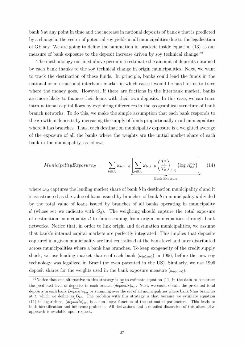
bank b at any point in time and the increase in national deposits of bank b that is predicted

by a change in the vector of potential soy yields in all municipalities due to the legalization

of GE soy. We are going to define the summation in brackets inside equation (13) as our

measure of bank exposure to the deposit increase driven by soy technical change.32

The methodology outlined above permits to estimate the amount of deposits obtained

by each bank thanks to the soy technical change in origin municipalities. Next, we want

to track the destination of these funds. In principle, banks could lend the funds in the

national or international interbank market in which case it would be hard for us to trace

where the money goes. However, if there are frictions in the interbank market, banks

are more likely to finance their loans with their own deposits. In this case, we can trace

intra-national capital flows by exploiting differences in the geographical structure of bank

branch networks. To do this, we make the simple assumption that each bank responds to

the growth in deposits by increasing the supply of funds proportionally in all municipalities

where it has branches. Thus, each destination municipality exposure is a weighted average

of the exposure of all the banks where the weights are the initial market share of each

bank in the municipality, as follows:

MunicipalityExposuredt =∑b∈Od

ωbd,t=0

[∑o∈Ob

ωbo,t=0

(T aoTo

)t=0

(logAsoyo,t

)]︸ ︷︷ ︸

Bank Exposure

(14)

where ωbd captures the lending market share of bank b in destination municipality d and it

is constructed as the value of loans issued by branches of bank b in municipality d divided

by the total value of loans issued by branches of all banks operating in municipality

d (whose set we indicate with Od). The weighting should capture the total exposure

of destination municipality d to funds coming from origin municipalities through bank

networks. Notice that, in order to link origin and destination municipalities, we assume

that bank’s internal capital markets are perfectly integrated. This implies that deposits

captured in a given municipality are first centralized at the bank level and later distributed

across municipalities where a bank has branches. To keep exogeneity of the credit supply

shock, we use lending market shares of each bank (ωbd,t=0) in 1996, before the new soy

technology was legalized in Brazil (or even patented in the US). Similarly, we use 1996

deposit shares for the weights used in the bank exposure measure (ωbo,t=0).

32Notice that one alternative to this strategy is be to estimate equation (11) in the data to construct

the predicted level of deposits in each branch ( deposits)bot. Next, we could obtain the predicted total

deposits in each bank Depositsbot by summing over the set of all municipalities where bank b has branchesat t, which we define as Obt. The problem with this strategy is that because we estimate equation

(11) in logarithms, ( deposits)bot is a non-linear function of the estimated parameters. This leads toboth identification and inference problems. All derivations and a detailed discussion of this alternativeapproach is available upon request.

27

V.D Capital reallocation towards destination municipalities: Empirical

Results

In this section we study the effect of municipality exposure as described in equation

(14) on aggregate bank lending and credit market participation in destination municipal-

ities. To this end, we estimate the following equation:

ydt = αd + αt + βMunicipalityExposuredt + εdt (15)

We focus on two main outcome variables: total bank lending and the share of bank

lending to non-agricultural sectors in destination municipality d and year t. Data on bank

lending is from the ESTBAN dataset and covers the years 1996 to 2010, the same time

span and set of municipalities covered in section V.B where we studied the local effects

of soy technical change on deposits and lending.

Table IV reports the results of estimating equation (15). We find that municipalities

with larger exposure to the soy-driven deposit increase through the bank network experi-

enced a larger increase in aggregate lending. The magnitude of the estimated coefficient

reported in column 1 implies that a municipality with a one standard deviation larger ex-

posure experienced around 7% larger increase in aggregate lending. This result is driven

by non-soy producing destination municipalities. In columns 2 and 3, we split the sample

in soy-producing and non-soy producing municipalities.33 Each of these groups accounts

for around half of the observations used in column 1. The estimated coefficient in the

soy-producing sample is 0.054 and not statistically significant, while the estimated coef-

ficient on the non-soy producing sample is 0.580 and strongly significant. These results

indicate a reallocation of capital towards non-soy producing regions.

Next we study whether this increase in lending has been directed towards agricultural

or non-agricultural sectors. The results of estimating equation (15) when the outcome

variable is the share of lending outside of the agricultural sector is reported in column

4. We find that municipalities with a one standard deviation larger exposure to the soy-

driven deposit boom experienced 2.2 percentage points larger increase in non-agricultural

lending as a share of total lending. This effect is largely concentrated in non-soy producing

region, as shown in columns 5 and 6.

The findings discussed above are consistent with the capital supply mechanism em-

phasized by the model: agricultural technical change can increase savings and lead to a

reallocation of capital towards the capital intensive sector, manufacturing. Our empirical

analysis permits to quantify this effect by comparing the speed of capital reallocation

across sectors in non-soy producing municipalities with different degrees of financial inte-

33Non-soy producing municipalities are those with no agricultural area farmed with soy at any pointin time between 1996 and 2010.

28

gration with the soy boom area. During the period under study (1996-2010), the share

of non-agricultural lending increased from 74.6 to 83.5 percent in the average non-soy

producing municipality. However, the degree of capital reallocation away from agricul-

ture varied extensively across municipalities: the interquartile range was 23 percentage

points. Our estimates imply that the differences in the degree of financial integration with

the soy boom area can explain 15 percent of the observed differences in the increase in

non-agricultural lending share across non-soy producing municipalities.

Overall, these results indicate that new agricultural technologies can generate struc-

tural transformation in regions not directly affected by the new technologies. Two caveats

with this specification are in order. First, this specification does not allow us to disentangle

the direct effect of capital reallocation from the labor supply or product demand channels

of agricultural productivity growth. For example, destination municipalities served by

more exposed banks might also be better connected to soy-producing regions through

transportation or migrant networks. Therefore, in section V.E, we propose an identifica-

tion strategy that aims at disentangling the capital supply channel from other channels

using loan-level and firm-level data. Second, the ESTBAN dataset used to construct the

agricultural and non-agricultural lending shares used as outcomes in this section includes

lending to both firms and individuals. Therefore, in section V.F, we use loan-level data

to more precisely identify credit flows to firms in different sectors.

Finally, in Table V, we study the effect of destination municipality exposure on credit

market participation. As shown in section IV.A.1, Brazil experienced a large increase in

the share of firms with access to bank credit during the period under study. To this end,

we estimate a version of equation 15 where the outcome variable is the share of firms

with access to bank credit in destination municipality d and year t.34 Given the effect of

municipality exposure on aggregate lending is concentrated in non-soy producing regions,

we estimate this equation exclusively on non-soy producing municipalities. We find that

municipalities with larger exposure to the soy boom through the bank network experience

larger increase in firm access to bank credit. The magnitude of the estimated coefficient

reported in column 1 implies that a municipality with a one standard deviation larger

exposure to the soy-driven deposit increase experienced a 0.3 percentage points larger

increase in the share of firms with access to bank credit. The average credit participation

across municipalities in our sample is 5.6%, which implies that a one standard deviation

increase in exposure would increase credit participation in the average municipality from

5.6% to 5.9%.35 In columns 2 and 3, we report the results of estimating the same equation

34We define access to bank credit using the 50,000 1997 R$ threshold in the Credit Information System.Under this definition, a firm is considered as having access to bank credit if its outstanding loan balancewith a bank in a given year is greater or equal to 50,000 1997 BRL.

35Notice that the average credit market participation across municipalities is slightly lower than thecredit market participation at national level reported in Figure II. This is because municipalities areequally weighted in Table V, and municipalities with a larger number of firms tend to be more urban andfinancially developed.

29

when the outcome variable is the share of firms with access to bank credit in different

firm size categories: micro and small firms in column 2, medium and large in column 3,

all defined as in section IV. Here we find the effect of municipality exposure on access to

bank credit is concentrated exclusively in micro and small firms.

V.E Capital reallocation towards destination firms: Empirical Strat-

egy

The findings presented in section V.D are consistent with the capital supply mecha-

nism emphasized by the model. However, to the extent that destination municipalities

which are more connected to origin municipalities through bank-branch networks are also

more connected through the transportation or commercial networks, it is possible that

our estimates are capturing the effects of agricultural technical change through the la-

bor supply or product demand channels. To make progress on this front, in this section

we propose a different empirical strategy which permits to control for labor supply and

product demand shocks in destination municipalities. In particular, we trace the reallo-

cation of capital towards firms located in destination municipalities. For this purpose, we

match administrative data on the credit and employment relationships for the universe

of formal firms. We use this data to construct firm-level exogenous credit supply shocks

using information on pre-existing firm-bank relationships. We use these shocks to assess

whether firms whose pre-existing lenders are more connected to soy-producing regions

through bank branch networks experienced larger increases in borrowing and employ-

ment growth. This empirical strategy permits to compare firms operating in the same

sectors and municipality but initially borrowing from different banks. This allows to con-

trol for labor supply and product demand shocks in destination municipalities and thus

isolate the capital supply channel. In what follows we explain this identification strategy

in more details.

We start by characterizing the relationship between bank deposits and firm borrowing.

To this end, we assume that loans of firm i from bank b are described as follows:

loansibt= I ibtrλbtubit

where Iibt is an indicator variable taking the value of one when there is a bank-firm

relationship. In turn, rbt is the interest rate, which varies across banks due to internal

capital markets: we assume that it is cheaper to finance loans with deposits than other

sources such as the interbank market. To proceed with estimation, we first condition on

the sample with Iib,t=0 > 0 – i.e. we condition on pre-existing bank-firm relationships –

and take logs to obtain:

log(loansibt) = δi + δt + δb + λ log rbt + εbit (16)

30

Note that because we condition on Iib,t=0 > 0, our estimates on this sample of firms only

capture the ”intensive margin.” That is, we only analyze the increase in lending from

banks with whom firms had pre-existing relationships.

Second, we assume that differences in interest rates across banks are partly determined

by deposits due to internal capital markets:

log rbt = ρt + ρb + µ logDepositsbt + υbt

Third, we substitute the equation above on equation (16) to obtain our main estimating

equation:

log(loansibt) = δi + δt + δb + λµ logDepositsbt + ebit (17)

The equation above shows that exogenous increases in deposits can generate larger

loans if λµ > 0: firms borrow more when the interest rate falls and banks increase their

lending when they receive more deposits due to frictions in the interbank market. To

identify λµ we use the exogenous increases in deposits generated by soy technical change

– our measure of bank exposure as defined in equation (13).

We therefore substitute equation (13) in our structural equation of interest (17), to

obtain:

log(loansibt) = νi + νt + νb + βBankExposurebt + εbit (18)

where:

νi = δi;

νt = δt + λµγt;

νb = δb + λµγb;

BankExposurebt =∑o∈Ob

ωbo,t=0

(T aoTo

)t=0

(logAo,t) .

and

Asoyot =

Asoy,LOWo for t < 2003

Asoy,HIGHo for t ≥ 2003

This estimation strategy allows to identify the parameter β = λµ under the assumption

that the soy driven credit supply change at the bank-level is uncorrelated with credit

demand changes at the firm-level.

Our identification assumption could be violated in the following cases. First, if firms

credit demand grows because they face larger demand from richer soy farmers or face larger

labor supply from former agricultural workers. To address this concern, we restrict our

31

sample to firms operating in non-soy producing municipalities, that is, municipalities that

do not produce soy at any point during the period under study. Second, if firms supply

or buy inputs for soy production. To address this concern, we exclude firms operating

in sectors directly linked to soy production through input-output linkages. This includes

firms operating in the food processing industry, and firms operating in manufacturing

sectors producing chemicals used as inputs in agriculture such as insecticides, herbicides,

and fungicides.

A broader related concern is that different industries might be on differential growth

trends due to other changes in the world economy such as increased trade with China.

To address this concern, we include interactions of industry and time dummies in our

specification.36 A third concern is that the bank branch network connects municipalities

that are also better connected through the transportation network. Thus, even if they do

not produce soy they might be affected by in-migration or demand linkages. To address

this concern, we estimate a specification where we control for an interaction of municipality

and time dummies which absorb all the municipality-level variation across time. We then

estimate the following specification:

log(loansidsbt) = νi + νb + νdt + νst + βBankExposurebt + εbit (19)

where the subindex d denotes the destination municipality, that is the municipality where

the firm is located, and s the industry in which the firm operates.37 In turn, νdt are

destination municipality interacted with time fixed effects, and νst are industry interacted

with time fixed effects.

In addition to study the effect of capital reallocation on firm borrowing, we are also

interested in assessing the real effects of this additional borrowing. In particular, we want

to understand the extent to which firms use additional credit to finance growth enhancing

investments. These investments can take the form of expanding the use of capital, labor

or other inputs. Because in the RAIS dataset we observe labor and the wage bill, we focus

our analysis on these two inputs. However, we think that to the extent that there is some

complementarity between production inputs, we expect that any investment leading to

expansion of the firm is likely to be reflected in larger employment and wage bill. Thus,

we analyze real effects through the following firm-level specification:

log(yidst) = νi + νdt + νst + βFirmExposureit + εbit (20)

36We use 2-digit sectors in the CNAE 1.0 Brazilian Industry Classification to construct this set of fixedeffects

37Sector fixed effects are 2-digits sectors according to the Brazilian CNAE 1.0 classification. Firms inour sample are present in 56 2-digit CNAE 1.0 sectors.

32

where:

FirmExposureit =∑b∈B

πib,t=0 BankExposurebt

and

πib,t=0 =loansib,t=0

Loansi,t=0

The variable yidst denotes an outcome such as total wage bill or employment in firm i,

located in destination municipality d, operating in industry s at time t,. Our measure of

firm exposure is defined as a weighted average of bank exposure of all lenders with which

firm i had a credit relationship in the pre GE-soy legalization period, which correspond

to the years 2001 and 2002 in the Credit Registry Data. The weights correspond to the

share of borrowing of firm i from bank b in 2001 and 2002 as a share of total borrowing of

firm i in the same years. We use pre-existing bank relationships to minimize the concern

that endogenous formation of firm-bank relationships — which could depend from a bank

exposure to the soy boom — might affect our results. Notice that this implies that we use

the exposure of the pre-2003 lenders for all years in which a firm is present in our sample,

no matter whether the firm is borrowing or not from those lenders in the years after GE

soy legalization. Since the set of lenders used to construct this measure is defined in the

initial period and it is time invariant for each firm, the bank fixed effects νb are effectively

absorbed by firm fixed effects νi in this specification.

V.F Capital reallocation towards destination firms: Empirical Results

V.F.1 Bank aggregate deposits and exposure

In the following subsections we study whether larger increases in bank deposits due

to soy technical change affected credit supply and firm growth. Before presenting these

results, in this subsection we test the relationship between aggregate deposits of bank b

and the increase in aggregate deposits for the same bank that is predicted by our measure

of bank exposure. This relationship is described by equation 13 in section V.C, which we

report below for the reader’s convenience:

logDepositsbt = γb + γt + βBankExposurebt + ηbt (13)

Table VI reports the results of estimating equation (13) when the outcome variable

is aggregate deposits of bank b, and bank-year observations are weighted by initial bank

size.38 Aggregate deposits for each bank are obtained summing branch level deposits

from ESTBAN.39 The point estimate on BankExposure is positive and significant, which

indicates that banks more exposed to soy technical change through their branch network

38As captured by bank assets in the initial year.39We focus on the years 2001 to 2010 in order to match the same time period used in the firm-level

analysis presented in the next subsections.

33

experienced higher increase in aggregate deposits. The magnitude of the estimated coef-

ficient reported in column 1 is 1.42. It indicates that a 1 percent increase in aggregate

deposits of bank b predicted by the change in the vector of potential soy yields corre-

spond to a 1.42 percent increase in actual national deposits of the same bank. In other

words, changes in our measure of predicted deposits are associated with changes in actual

deposits of similar magnitude.40 Columns 2 to 4 show that this effect is not driven by

other initial bank characteristics such as bank size or the deposit-to-asset ratio. Finally,

in Figures VIII (a) and (b) we report partial correlations between changes in bank expo-

sure and changes in the log of aggregate deposits at bank level, weighting and without

weighting by initial bank size respectively.41 As shown, our estimates are not driven by

extreme observations or weighting by bank size.

V.F.2 Bank-firm level specification

In this section we study the effect of the soy-driven increase in deposits of a given

bank – our measure of bank exposure – on firm borrowing from that same bank.42

Table VII shows the results of estimating equation (19), described in section V.E and

reported below for convenience:

log(loansibdst) = νi + νb + νdt + νst + βBankExposurebt + εbit (20)

where i indexes firms, b indexes banks, d indexes the destination municipality where the

firm is located, s indexes sectors, and t indexes time. The outcome variable is the log of

the monetary value of outstanding loan balance of firm i from bank b. The coefficient of

interest in this specification is the one on bank exposure (β), which captures the effect of

exposure of bank b on the outstanding loan balance of firm i from the same bank.

Table VII reports the estimated β. We start by estimating equation (19) in a specifi-

cation with firm, bank and time fixed effects in column 1. The estimated coefficient on the

variable BankExposure is positive, indicating that firms with pre-existing relationships

with more exposed banks experienced a larger increase in borrowing from those banks.

40We think that one reason why our estimate of β is larger than one is that our measure of Bankexposure is a first order approximation to changes in aggregate deposits holding the bank branch networkconstant. Thus, changes in the bank branch network are in the error term. It is very likely that the soyboom might have led banks to open new branches which capture deposits. Thus, our measure of bankexposure might underestimate the effect of the soy shock on aggregate deposits.

41This is equivalent to a first difference version of equation (13) obtained after partialling out year fixedeffects and bank initial characteristics interacted with linear time trends and then averaging bank exposureand log deposits for each bank in the years before (2001-2002) and after (2003-2010) the legalization ofGE soy seeds.

42We apply two restrictions to our sample. First, as explained in section V.E, we focus on firmsoperating in non-soy producing regions. Second, in order to minimize sample selection, we focus ouranalysis on the period 2001-2010, i.e. the years after the reporting threshold of the Credit Registry waslowered to 5,000 BRL. As shown in Figure II, in 2001 only around 7 percent of Brazilian firms had accessto finance when using the 50,000 BRL reporting threshold. In the same year, 31 percent of Brazilian firmshad access to finance under the 5,000 BRL reporting threshold, as shown in Figure A1 of the Appendix.

34

In column 2 we add municipality and sector fixed effects, both interacted with time fixed

effects. Notice that we find similar point estimates when controlling for municipality and

sector-level shocks. This suggests that the increase in firm borrowing is driven by the

capital supply effect of agricultural technical change and not the labor supply or product

demand effects. We can use this estimate to back out the implied elasticity of firm loans to

bank deposits due to the soy shock. In particular, we can divide the estimated coefficient

on bank exposure when the outcome is firm loans (0.277) by the estimated coefficient on

bank exposure when the outcome is bank deposits (1.43), to obtain 0.19. This implies that

1 extra dollar of bank deposits in origin municipalities due to the soy shock translated

into 19 extra cents lent to firms operating in non-soy producing municipalities.

In column 4 we augment equation (19) with firm fixed effects interacted with time fixed

effects. This specification fully captures firm-specific demand shocks (Khwaja and Mian

2008), and only exploits variation across banking relationships within firm to identify the

coefficient β. As a consequence, it can only be estimated using firms with multiple lending

relationships in both the pre and the post GE soy legalization period. The estimated

coefficient is positive, which implies that banks with larger exposure to the soy-driven

deposit shock relative to other banks also increased their lending by more to the same

firm. Notice also that the magnitude of the estimated coefficient is similar to the one

obtained without firm fixed effects interacted with time fixed effect on the same sample

of firms. This indicates that the effect of bank exposure on firm borrowing is driven by

credit supply forces rather than unobservable firm-specific demand shocks correlated with

lender exposure.43 Overall, the coefficients reported in Table VII support the validity of

our identification strategy.

Next, we study the effect of bank exposure on loans by sector of operation of the

borrowing firm. To this end, we estimate equation (19) separately for borrowers operating

in agriculture, manufacturing, services, and other sectors.44 Table VIII reports the results.

We find positive coefficients for firms in all sectors, with the largest and precisely estimated

effects in manufacturing and services. The magnitude of the estimated coefficients in

column 2 and 3 indicates an elasticity of firm loans to bank deposits due to the soy

shock of 0.21 in manufacturing and 0.19 in services. These elasticities are smaller and not

statistically significant in agriculture and other sectors (0.087 and 0.16 respectively).

Taking into account differences in average loan size and number of firms across sectors,

these estimates indicate that out of 1 R$ of new loans in destination municipalities from

43Under certain assumptions regarding the functional form of the underlying model describing borrow-ing of firm i from bank b, the difference in point estimates between specifications that include firm fixedeffects and those that do not captures the size of the bias induced by endogenous matching between firmsand banks (see Khwaja and Mian 2008).

44Services include: construction, commerce, lodging and restaurants, transport, housing services, do-mestic workers and other personal services. We exclude banks and other firms in the financial sector.Other sectors include: public administration, education, health, international organizations, extraction,and public utilities.

35

the soy-driven deposit shock, 0.5 cents were allocated to firms in agriculture, 40 cents to

firms in manufacturing, 47.7 cents to firms in services and 11.8 cents to firms in other

sectors.45

Overall, the results presented in this section indicate that firms with pre-existing

relationships with banks that were more exposed to the soy-driven increase in deposits

in origin municipalities experienced a larger increase in borrowing from those banks. In

addition, these results show that new capital originated from the soy-driven increase in

deposits and reallocated to non-soy producing regions through the bank branch network

was mostly lent to firms in manufacturing and services.

V.F.3 Firm level specification: real effects

In the previous section we showed that firms with pre-existing relationships with more

exposed banks experienced a larger increase in borrowing from those banks. In this section

we study the effect of firm exposure to the soy shock through all their pre-existing bank

relationships on firm growth. To this end, we estimate equation (20), as described in

section V.E and reported below for convenience:

log(yidsbt) = νi + νt + νb + νdt + νst + βBankExposurebt + εbit (21)

In terms of firm-level outcomes, we focus on two main variables: employment, defined

as the log of the yearly average number of workers; and wage bill, defined as the log of

the monetary value of the firm total wage bill. The results are reported in Table IX.

We find positive real effects on firm size. Firms whose pre-existing lenders have a larger

exposure to the soy-driven deposit increase experienced a larger growth in employment

and wage bill. In contrast with the loan estimates discussed in subsection V.F.2, we find

that our estimated real effects fall to almost half when we control for municipality and

sector-level shocks. This can be seen, for example, by comparing columns 1 and 2 in

Table IX. The coefficient on firm exposure when the outcome is employment goes from

0.281 to 0.165 when adding municipality and sector fixed effects interacted with year fixed

effects. This finding indicates that municipalities more connected through bank branch

networks might also be more connected through transportation or commercial networks,

thus are more likely to receive not only capital supply shocks but also labor supply and

product demand shocks due to agricultural productivity growth. As a result, firm-loan-

45This quantification is obtained as follows. First, we multiply the estimated coefficient on bankexposure by the average loan size in the years 2001 and 2002 in each sector. This gives us the estimatedincrease in loan size for the average firm in each sector, in response to a unit increase in exposure ofits main lender. Second, we multiply this estimate by the average number of firms operating in eachsector in destination municipalities in our sample in the years 2001 and 2002. This multiplication givesus an estimate of the total increase in the value of loans of firms in each sector in response to a unitincrease in exposure of their lenders. Finally, we use these estimates of total increase in loan value ineach sector to compute the allocation across-sectors of 1 R$ of new loans in destination municipalitiesfrom the soy-driven deposit shock.

36

level data is necessary to separately identify the effects of the capital supply channel on

the allocation of labor across sectors. In terms of magnitudes, when we focus on the

estimates presented in columns 2 and 4, the estimated coefficients indicate that a firm

whose pre-existing lenders have a 1 standard deviation higher increase in deposits due to

soy technical change experienced a 3.8% larger increase in employment and a 5.2% larger

increase in wage bill.

Next, we estimate the same equation by sector of operation of each firm. Table X

reports the results. As shown, the average effects of firm exposure on firm size are pos-

itive and similar in size in agriculture, manufacturing and services, while small and not

statistically significant for firms operating in other sectors. These estimates, along with

differences in average firm size and number of firms in each sector, can be used to compute

the allocation of extra workers across sectors for a given increase in firm exposure. Our

estimated coefficients indicate that out of 100 additional workers in destination munic-

ipalities due to the soy-driven deposit shock, 1.7 were employed in agriculture, 32.1 in

manufacturing, 62.6 in services and 3.6 in other sectors. To sum up, our results indi-

cate that reallocation of capital from origin to destination municipalities had real effects

on employment, and these effects were concentrated in the manufacturing and services

sectors.

VI Concluding Remarks

This paper studies the effect of agricultural productivity on structural transformation

in open economies through its impact on capital accumulation. The empirical analysis

is focused on the widespread adoption of genetically engineered soy in Brazil. This new

technology allows farmers to obtain the same yield with lower production costs, thus

increasing agricultural profits. The effect of the new agricultural technology on structural

transformation via capital accumulation depends on several features of the environment.

First, the relative strength of the demand and supply effects of agricultural technical

change, which, as highlighted in our model, work in opposite directions. The finding that

the adoption of genetically engineered soy seeds generated more profits than investment in

agriculture suggests that the supply effect dominates. Indeed, we find a positive effect of

GE soy adoption on deposits in local bank branches. In this case, the model predicts that

capital reallocates towards non-agricultural sectors. Because in our setting soy producing

regions tend to be rural, this reallocation needs to take place both across sectors and

regions. Indeed, branches located in soy producing areas were net capital exporters within

their bank network, and capital was reallocated towards other regions. Thus, a second

key feature of the environment is the degree of financial integration across regions. We

find that regions more financially integrated with the soy boom area experience faster

structural transformation. In particular, banks experiencing faster deposit growth in

37

soy areas increased their lending to firms with whom they had preexisting relationships.

In turn, these firms grew faster in terms of employment and wage bill. Real effects

were concentrated in non-agricultural sectors. These findings indicate that agricultural

productivity growth can lead to structural transformation through its impact on capital

accumulation.

38

References

Acemoglu, D. and V. Guerrieri (2008). Capital deepening and nonbalanced economicgrowth. Journal of political Economy 116 (3), 467–498.

Acemoglu, D. and F. Zilibotti (1997). “Was Prometheus Unbound by Chance? Risk,Diversification, and Growth”. Journal of political economy 105 (4), 709–751.

Banerjee, A., D. Karlan, and J. Zinman (2001). Six randomized evaluations of microcredit:Introduction and further steps. American Economic Journal: Applied Economics 7 (1),1–21.

Banerjee, A. and K. Munshi (2004). “How Efficiently is Capital Allocated? Evidence fromthe Knitted Garment Industry in Tirupur”. The Review of Economic Studies 71 (1),19–42.

Banerjee, A. V. and E. Duflo (2014). Do firms want to borrow more? testing creditconstraints using a directed lending program. Review of Economic Studies 81 (2), 572–607.

Banerjee, A. V., E. Duflo, R. Glennerster, and C. Kinnan (2013). The miracle of micro-finance? evidence from a randomized evaluation.

Banerjee, A. V. and A. F. Newman (1993). “Occupational Choice and the Process ofDevelopment”. Journal of political economy , 274–298.

Bryan, G. and M. Morten (2015). Economic development and the spatial allocation oflabor: Evidence from indonesia. Manuscript, London School of Economics and StanfordUniversity .

Buera, F. J., J. P. Kaboski, and Y. Shin (2015). “Entrepreneurship and Financial Fric-tions: A Macro-Development Perspective”.

Bustos, P., B. Caprettini, and J. Ponticelli (2016). “Agricultural productivity and struc-tural transformation: Evidence from Brazil”. The American Economic Review 106 (6),1320–1365.

Chodorow-Reich, G. (2014). “The employment effects of credit market disruptions:Firm-level evidence from the 2008–9 financial crisis”. The Quarterly Journal of Eco-nomics 129 (1), 1–59.

Cole, S. (2009). Financial development, bank ownership, and growth: Or, does quantityimply quality? The Review of Economics and Statistics 91 (1), 33–51.

Corden, W. M. and J. P. Neary (1982). “Booming Sector and De-Industrialization in aSmall Open Economy”. The Economic Journal 92 (368), 825–848.

Crafts, N. F. (1985). British economic growth during the industrial revolution. ClarendonPress Oxford.

Crouzet, F. (1972). Capital Formation in the Industrial Revolution. Methuen.

De Mel, S., D. McKenzie, and C. Woodruff (2008). Returns to capital in microenterprises:evidence from a field experiment. The Quarterly Journal of Economics , 1329–1372.

39

Donaldson, D. (2015). Railroads of the raj. American Economic Review, forthcoming .

Donaldson, D. and R. Hornbeck (2016). Railroads and american economic growth: A“market access” approach. The Quarterly Journal of Economics 131 (2), 799–858.

Duffy, M. and D. Smith (2001). “Estimated Costs of Crop Production in Iowa”. IowaState University Extension Service FM1712.

Fajgelbaum, P. and S. J. Redding (2014). External integration, structural transformationand economic development: Evidence from argentina 1870-1914. Technical report,National Bureau of Economic Research.

Fernandez-Cornejo, J., C. Klotz-Ingram, and S. Jans (2002). “Estimating Farm-LevelEffects of Adopting Herbicide-Tolerant Soybeans in the USA”. Journal of Agriculturaland Applied Economics 34, 149–163.

Findlay, R. (1970). “Factor Proportions and Comparative Advantage in the Long Run”.Journal of Political Economy 78 (1), 27–34.

Findlay, R. and H. Grubert (1959). “Factor Intensities, Technological Progress, and theTerms of Trade”. Oxford Economic Papers 11 (1), 111–121.

Foster, A. D. and M. R. Rosenzweig (2004). “Agricultural productivity growth, ruraleconomic diversity, and economic reforms: India, 1970–2000”. Economic Developmentand Cultural Change 52 (3), 509–542.

Foster, A. D. and M. R. Rosenzweig (2007). “Economic development and the decline ofagricultural employment”. Handbook of development economics 4, 3051–3083.

Galor, O. and J. Zeira (1993). “Income Distribution and Macroeconomics”. The reviewof economic studies 60 (1), 35–52.

Gilje, E., E. Loutskina, and P. E. Strahan (2013). “Exporting Liquidity: Branch Bankingand Financial Integration”. NBER Working paper .

Gine, X. and R. M. Townsend (2004). “Evaluation of financial liberalization: a gen-eral equilibrium model with constrained occupation choice”. Journal of DevelopmentEconomics 74 (2), 269–307.

Gollin, D., D. Lagakos, and M. E. Waugh (2014). “The Agricultural Productivity Gap”.Quarterly Journal of Economics .

Herrendorf, B., R. Rogerson, and A. Valentinyi (2013). Growth and Structural Transfor-mation. NBER Working Paper .

Huggins, D. R. and J. P. Reganold (2008). “No-Till: the Quiet Revolution”. ScientificAmerican 299, 70–77.

IBGE (2006). “Censo Agropecuario 2006”. Rio de Janeiro, Brazil: Instituto Brasileiro deGeografia e Estatıstica (IBGE).

Jeong, H. and R. M. Townsend (2008). “Growth and inequality: Model evaluation basedon an estimation-calibration strategy”. Macroeconomic dynamics 12 (S2), 231–284.

40

Khwaja, A. I. and A. Mian (2008). Tracing the impact of bank liquidity shocks: Evidencefrom an emerging market. The American Economic Review , 1413–1442.

Marden, S. (2016). The agricultural roots of industrial development: forward linkages inreform era china. Working Paper .

Matsuyama, K. (1992). “Agricultural Productivity, Comparative Advantage, and Eco-nomic Growth”. Journal of economic theory 58 (2), 317–334.

McCaig, B. and N. Pavcnik (2013). Moving out of agriculture: structural change invietnam.

McKenzie, D. and C. Woodruff (2008). Experimental evidence on returns to capital andaccess to finance in mexico. The World Bank Economic Review 22 (3), 457–482.

Michaels, G., F. Rauch, and S. J. Redding (2012). Urbanization and structural transfor-mation. The Quarterly Journal of Economics 127 (2), 535–586.

Moll, B. (2014). Productivity losses from financial frictions: Can self-financing undocapital misallocation? The American Economic Review 104 (10), 3186–3221.

Moll, B., R. M. Townsend, and V. Zhorin (2017). Economic development, flow of funds,and the equilibrium interaction of financial frictions. Proceedings of the NationalAcademy of Sciences , 201707055.

Moretti, E. (2011). Local labor markets. Handbook of labor economics 4, 1237–1313.

Munshi, K. and M. Rosenzweig (2016). Networks and misallocation: Insurance, migration,and the rural-urban wage gap. The American Economic Review 106 (1), 46–98.

Murphy, K. M., A. Shleifer, and R. Vishny (1989). Income distribution, market size, andindustrialization. The Quarterly Journal of Economics 104 (3), 537–564.

Nurkse, R. (1953). Problems of Capital Formation in Underdeveloped Countries. OxfordUniversity Press.

Rosenstein-Rodan, P. N. (1943). Problems of Industrialization of Eastern and South-Eastern Europe. Economic Journal 53, 202–211.

Rostow, W. (1960). The Stages of Economic Growth: A Non Communist Manifesto.Cambridge University Press, London.

Rybczynski, T. M. (1955). “Factor Endowment and Relative Commodity Prices”. Eco-nomica 22 (88), 336–341.

Stiglitz, J. E. (1970). “Factor Price Equalization in a Dynamic Economy”. Journal ofPolitical Economy 78 (3), 456–488.

USDA (2012). “Agricultural Biotechnology Annual”. United States Department of Agri-culture, Economic Research Service.

Ventura, J. (1997). “Growth and Interdependence”. The Quarterly Journal of Eco-nomics 112 (1), 57–84.

41

Figures and Tables

Figure I: Evolution of Area Planted with Soy in Brazil

510

1520

area

(m

illio

n ha

)

1980 1990 2000 2010

year

Notes: Data source is CONAB, Companhia Nacional de Abastecimento, which is an agency within the Brazilian Ministryof Agriculture. CONAB carries out monthly surveys to monitor the evolution of the harvest of all major crops in Brazil:the surveys are representative at state level and are constructed by interviewing on the ground farmers, agronomists andfinancial agents in the main cities of the country.

Figure II: Share of Firms with Bank CreditBrazil: 1997-2010

1.4m

2.5m

7%

14%

0.1

.2.3

.4S

hare

of f

irms

with

ban

k cr

edit

01

23

N fi

rms

(mill

ion)

1997

1998

1999

2000

2001

2002

2003

2004

2005

2006

2007

2008

2009

2010

N firms Share of firms with bank credit

Notes: Sources are the Credit Information System of the Central Bank of Brazil and RAIS. Authors’ calculation frommicro-data. Access to bank credit is defined as an outstanding credit balance with a financial institution of at least 50,0001997 BRL.

42

Figure III: Share of Firms with Bank Credit: by SectorBrazil: 1997-2010

18%

15%14%

24%

5%

13%

0.1

.2.3

Sha

re o

f firm

s w

ith b

ank

cred

it

1997

1998

1999

2000

2001

2002

2003

2004

2005

2006

2007

2008

2009

2010

agriculture manufacturing

services

Notes: Sources are the Credit Information System of the Central Bank of Brazil and RAIS, authors’ calculation from micro-data. Access to bank credit is defined as an outstanding credit balance with a financial institution of at least 50,000 1997BRL. Services include: construction, commerce, lodging and restaurants, transport, housing services, domestic workers.

Figure IV: Share of Firms with Bank Credit: by Firm SizeBrazil: 1997-2010

3%

9%

18%

34%

45%54%

60%63%

0.1

.2.3

.4.5

.6.7

Sha

re o

f firm

s w

ith b

ank

cred

it

1997

1998

1999

2000

2001

2002

2003

2004

2005

2006

2007

2008

2009

2010

micro L=1-9 (84.1%) small L=10-49 (12.7%)

medium L=50-99 (1.5%) large L=100+ (1.7%)

Notes: Sources are the Credit Information System of the Central Bank of Brazil and RAIS, authors’ calculation frommicro-data. Access to bank credit is defined as an outstanding credit balance with a financial institution of at least 50,0001997 BRL. Numbers in parenthesis are the percentage of firms in each size category in 1997.

43

Figure V: Potential soy yield under low agriculturaltechnology

Notes: Data source is FAO-GAEZ. Units are tons per hectare.

Figure VI: Potential soy yield under highagricultural technology

Notes: Data source is FAO-GAEZ. Units are tons per hectare.

44

Figure VII: Bank Networks and Increase in Soy Revenues

(a) Bank A

(2.73,14.37](0.98,2.73](0.35,0.98](-0.03,0.35][-8.08,-0.03]no soy production

(b) Bank B

(8.39,14.22](4.70,8.39](1.86,4.70](0.70,1.86][-5.27,0.70]no soy production

Notes: Data sources are ESTBAN for bank branch location and the Municipal Agricultural Production Survey for revenues from soy production.

45

Figure VIII: Bank Deposits and Bank Exposure

(a) Partial Correlation, Weighted by Bank Size

-6-4

-20

24

Dep

osit

Gro

wth

(log

)

-.4 -.2 0 .2 .4Bank Exposure

(b) Partial Correlation, Unweighted

-6-4

-20

24

Dep

osit

Gro

wth

(log

)

-.4 -.2 0 .2 .4Bank Exposure

Notes: The graphs show the partial correlations between changes in bank exposure and changes in log deposits at bank level. Changes are computed after averaging bank exposure and log

deposits for each bank before (2001-2002) and after (2003-2010) the legalization of GE soy seeds. Bank exposure and log deposits are averaged after partialling out year fixed effects, as well

as log of bank assets and deposit-to-asset ratio (both observed in 1996) interacted with linear time trends. This is therefore equivalent to a first difference version of equation (13). The results

of estimating equation (13) in levels are reported in Table VI, column 4. In these graphs we focus on bank exposure values (after partialling out fixed effects and bank controls) between -0.5

and +0.5. This is for a more transparent visualization of the data and has negligible effects on the slope of the regression. The estimated slope using the same 121 banks as in Table VI is 1.81

(t-stat = 2.25), while if we focus on bank exposure values between -0.5 and +0.5 (N=114), the estimated slope is 2.12 (t-stat=2.44). Panel (b) reports the unweighted version of Panel (a).

46

Table I: Summary Statistics

variable name mean st.dev. N

independent variables:∆log(Asoy

jt ) 1.917 0.466 3,020

log(Asoyjt ) -0.285 1.136 44,406

MunicipalityExposure -0.041 0.242 44,406BankExposure 0.069 0.198 1,052

outcome variables at municipality-level: ahksadhf

∆GESoyAreaAgriArea 0.015 0.064 3,020

∆Agri Productivity 0.504 0.695 3,020∆Agri Profits per he (pct points) 0.319 1.867 3,020∆Agri Investment per he (pct points) 0.475 1.042 3,020Soy Area / Agricultural Area 0.051 0.136 44,406log(deposits) 15.693 1.809 44,406log(loans) 15.459 2.112 44,406(deposits - loans) / assets 0.811 1.977 44,406Non-agricultural loans / total loans 0.690 0.275 44,406Bank credit participation 0.056 0.058 26,897

outcome variables at loan-levellog(loan)

All sectors 10.374 1.777 2,795,805All sectors - multi-lender firms 10.680 1.843 1,646,097Agriculture 11.206 2.055 12,588Manufacturing 10.939 1.933 581,003Services 10.208 1.684 2,057,719Other 10.446 1.911 130,985

outcome variables at firm-level:log employment

All sectors 2.067 1.467 1,730,753Agriculture 2.790 1.674 6,188Manufacturing 2.665 1.445 303,871Services 1.879 1.402 1,318,234Other 2.761 1.665 84,328

log wage billAll sectors 8.387 1.722 1,730,753Agriculture 8.966 1.871 6,188Manufacturing 9.145 1.710 303,871Services 8.160 1.637 1,318,234Other 9.148 1.983 84,328

Notes: All variables are winsorized at 1% in each tail. See section IV for a detailed description

of data sources.

47

Table II: Soy Technical Change and Agricultural Census OutcomesGE Soy Adoption, Agricultural Productivity, Profits and Investment per hectare

∆ Agricultural ∆ Profits ∆ Investment

outcome: GE Soy AreaAgricultural Area Productivity per he (%) per he (%)

(1) (2) (3) (4) (5) (6) (7) (8)

∆ logAsoy 0.039*** 0.033*** 0.119*** 0.116*** 0.259*** 0.229*** 0.181*** 0.214***[0.003] [0.003] [0.028] [0.031] [0.071] [0.079] [0.044] [0.048]

rural popt=1991 y y y y y y y yAMC controlst=1991 y y y y

Observations 3,020 3,020 3,020 3,020 3,020 3,020 3,020 3,020R-squared 0.082 0.152 0.009 0.011 0.004 0.014 0.014

Notes: The outcomes in this table are sourced from the Agricultural Censuses of 1996 and 2006. We thus estimate a first-difference version of equation (7):

∆yj = ∆α+ β∆ log(Asoyj ) + ∆εj

where the outcome of interest, ∆yj is the change in outcome variables between the last two census years and ∆ log(Asoyj ) = log(Asoy,HIGHj ) − log(Asoy,LOWj ).

Robust standard errors reported in brackets. Significance levels: *** p<0.01, ** p<0.05, * p<0.1. The variable rural pop is the share of rural adult population in

an AMC according to the 1991 Population Census. AMC controls include: income per capita (in logs), population density (in logs), literacy rate, all observed in

1991 (source: Population Census). AMC stands for Minimum Comparable Area (Area Mınima Comparavel). AMCs are composed by one or more municipalities

and are defined by the Brazilian Statistical Institute (IBGE) as geographical units of observation that can be compared over time.

48

Table III: Local Effects of Soy Technical ChangeSoy Area Share, Deposits, Lending and Capital Export

outcome: Soy AreatAgri Areat=1996

log(deposits) log(loans) deposits−loansassets

(1) (2) (3) (4) (5) (6) (7) (8)

logAsoy 0.021*** 0.017*** 0.060*** 0.070*** -0.077*** -0.061** 0.305*** 0.297***[0.002] [0.002] [0.016] [0.016] [0.029] [0.029] [0.062] [0.065]

AMC fe y y y y y y y yyear fe y y y y y y y yrural popt=1991 × year fe y y y y y y y yAMC controlst=1991 × year fe y y y y

Observations 44,406 44,406 44,406 44,406 44,406 44,406 44,406 44,406R-squared 0.958 0.959 0.975 0.976 0.951 0.951 0.711 0.713N clusters 3145 3145 3145 3145 3145 3145 3145 3145

Notes: Standard errors clustered at AMC level are reported in brackets. Significance levels: *** p<0.01, ** p<0.05, * p<0.1. The variable rural pop is the share

of rural adult population in an AMC according to the 1991 Population Census. AMC controls include: income per capita (in logs), population density (in logs),

literacy rate, all observed in 1991 (source: Population Census). AMC stands for Minimum Comparable Area (Area Mınima Comparavel). AMCs are composed

by one or more municipalities and are defined by the Brazilian Statistical Institute (IBGE) as geographical units of observation that can be compared over time.

49

Table IV: Capital Reallocation Across MunicipalitiesLending and Non-Agricultural Lending Share

outcome: log(loans) non-agricultural loanstotal loans

sample: all soy non-soy all soy non-soyregion region region region

(1) (2) (3) (4) (5) (6)

MunicipalityExposuredt 0.283*** 0.054 0.580*** 0.090*** 0.046* 0.139***[0.090] [0.124] [0.131] [0.016] [0.024] [0.023]

AMC fe y y y y y yyear fe y y y y y yrural popt=1991 × year fe y y y y y yAMC controlst=1991 × year fe y y y y y y

Observations 44,406 22,550 21,856 44,406 22,550 21,856R-squared 0.952 0.949 0.953 0.843 0.846 0.779N clusters 3145 1565 1580 3145 1565 1580

Notes: Standard errors clustered at AMC level are reported in brackets. Significance levels: *** p<0.01, ** p<0.05, * p<0.1.The variable rural pop is the share

of rural adult population in an AMC according to the 1991 Population Census. AMC controls include: income per capita (in logs), population density (in logs),

literacy rate, all observed in 1991 (source: Population Census). AMC stands for Minimum Comparable Area (Area Mınima Comparavel). AMCs are composed

by one or more municipalities and are defined by the Brazilian Statistical Institute (IBGE) as geographical units of observation that can be compared over time.

50

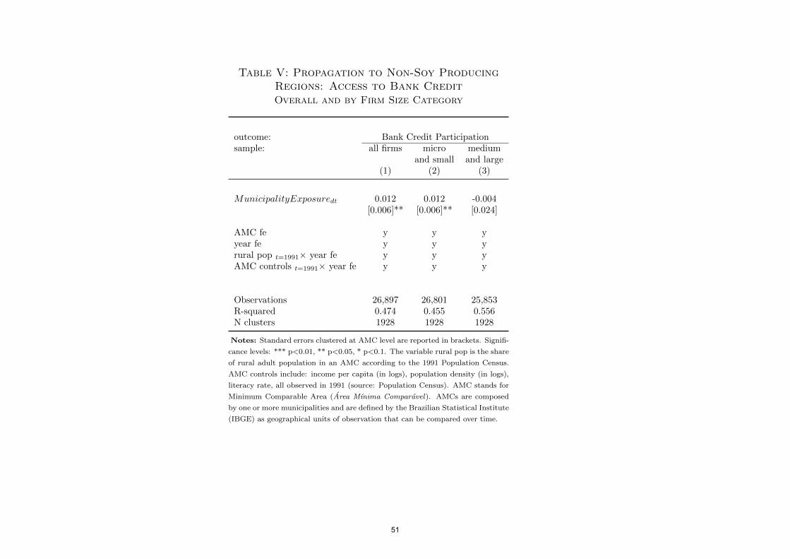
Table V: Propagation to Non-Soy ProducingRegions: Access to Bank CreditOverall and by Firm Size Category

outcome: Bank Credit Participationsample: all firms micro medium

and small and large(1) (2) (3)

MunicipalityExposuredt 0.012 0.012 -0.004[0.006]** [0.006]** [0.024]

AMC fe y y yyear fe y y yrural pop t=1991× year fe y y yAMC controls t=1991× year fe y y y

Observations 26,897 26,801 25,853R-squared 0.474 0.455 0.556N clusters 1928 1928 1928

Notes: Standard errors clustered at AMC level are reported in brackets. Signifi-

cance levels: *** p<0.01, ** p<0.05, * p<0.1. The variable rural pop is the share

of rural adult population in an AMC according to the 1991 Population Census.

AMC controls include: income per capita (in logs), population density (in logs),

literacy rate, all observed in 1991 (source: Population Census). AMC stands for

Minimum Comparable Area (Area Mınima Comparavel). AMCs are composed

by one or more municipalities and are defined by the Brazilian Statistical Institute

(IBGE) as geographical units of observation that can be compared over time.

51

Table VI: Bank Deposits and Bank Exposure

outcome: log deposits

(1) (2) (3) (4)

BankExposurebt 1.427** 1.664*** 1.580** 1.750**[0.587] [0.562] [0.761] [0.688]

Log Assetsb,t=0 × t -0.012 -0.010[0.010] [0.012]

Deposits/Assetsb,t=0 × t -0.085 -0.068[0.140] [0.151]

bank fe y y y yyear fe y y y y

Observations 1,052 1,052 1,052 1,052R-squared 0.913 0.913 0.913 0.913N clusters 121 121 121 121

Notes: Standard errors clustered at bank level are reported in brackets. Significance levels: *** p<0.01, ** p<0.05, *

p<0.1. Regressions are weighted by total bank assets in 1996. Bank controls are observed in 1996 (source: ESTBAN) and

interacted with linear time trends.

52

Table VII: The Effect of Bank Exposure on LoansLoan Value

outcome: log loan

multi-lender(1) (2) (3) (4)

BankExposurebt 0.245 0.277 0.271 0.211[0.118]** [0.106]*** [0.107]** [0.093]**

fixed effects:firm y y y yyear y y y ybank y y y yAMC × year y y ySector × year y y yfirm × year y

Observations 2,795,805 2,795,805 1,646,097 1,646,097R-squared 0.545 0.550 0.529 0.658N clusters 115 115 115 115

Notes: Standard errors clustered at bank level reported in brackets. Significance levels: *** p<0.01, ** p<0.05, *

p<0.1. AMC stands for Minimum Comparable Area (Area Mınima Comparavel). AMCs are composed by one or more

municipalities and are defined by the Brazilian Statistical Institute (IBGE) as geographical units of observation that can be

compared over time. Sector dummies correspond to the 87 2-digit sectors according to the Brazilian CNAE 2.0 classification.

53

Table VIII: The Effect of Bank Exposure on Loans by SectorLoan Value

outcome: log loan

Agriculture Manufacturing Services Other(1) (2) (3) (4)

BankExposurebt 0.125 0.304 0.266 0.228[0.211] [0.158]* [0.096]*** [0.177]

fixed effects:firm y y y yyear y y y ybank y y y yAMC × year y y y ySector × year y y y y

Observations 12,588 581,003 2,057,719 130,985R-squared 0.685 0.571 0.527 0.595N clusters 73 113 115 95

Notes: Standard errors clustered at bank level reported in brackets. Significance levels: *** p<0.01, ** p<0.05, *

p<0.1. AMC stands for Minimum Comparable Area (Area Mınima Comparavel). AMCs are composed by one or more

municipalities and are defined by the Brazilian Statistical Institute (IBGE) as geographical units of observation that can be

compared over time. Sector dummies correspond to the 87 2-digit sectors according to the Brazilian CNAE 2.0 classification.

54

Table IX: The Effect of Firm Exposure on Firm-level OutcomesEmployment and Wage Bill

outcome: log employment log wage bill

(1) (2) (3) (4)

FirmExposureit 0.281 0.165 0.437 0.226[0.044]*** [0.040]*** [0.055]*** [0.043]***

fixed effects:firm y y y yyear y y y yAMC × year y ySector × year y y

Observations 1,730,753 1,730,753 1,730,753 1,730,753R-squared 0.882 0.885 0.902 0.905N clusters 115 115 115 115

Notes: Standard errors clustered at main lender level reported in brackets. Significance levels: *** p<0.01, ** p<0.05, * p<0.1. AMC stands for Minimum

Comparable Area (Area Mınima Comparavel). AMCs are composed by one or more municipalities and are defined by the Brazilian Statistical Institute (IBGE)

as geographical units of observation that can be compared over time. Sector dummies correspond to the 87 2-digit sectors according to the Brazilian CNAE 2.0

classification.

55

Table X: The Effect of Firm Exposure on Firm-level Outcomes - BySector

Employment and Wage Bill

outcome: log employment log wage billindep var: FirmExposureit

(1) (2)

Agriculture 0.253 0.282[0.149]* [0.139]**

Observations 6,188 6,188R-squared 0.935 0.945N clusters 55 55

Manufacturing 0.202 0.309[0.050]*** [0.056]***

Observations 303,871 303,871R-squared 0.890 0.913N clusters 103 103

Services 0.162 0.211[0.039]*** [0.040]***

Observations 1,318,234 1,318,234R-squared 0.875 0.896N clusters 112 112

Other 0.024 0.108[0.064] [0.085]

Observations 84,328 84,328R-squared 0.939 0.948N clusters 79 79

fixed effects in all specificationsfirm y yyear y yAMC × year y ySector × year y y

Notes: Standard errors clustered at main lender level reported in brackets. Significance levels: *** p<0.01, ** p<0.05,

* p<0.1. AMC stands for Minimum Comparable Area (Area Mınima Comparavel). AMCs are composed by one or more

municipalities and are defined by the Brazilian Statistical Institute (IBGE) as geographical units of observation that can be

compared over time. Sector dummies correspond to the 87 2-digit sectors according to the Brazilian CNAE 2.0 classification.

56

Appendix

Figure A1: Share of Firms with Bank CreditBrazil: 2001-2010

1.6m

2.5m

31%

43%

0.1

.2.3

.4.5

.6.7

.8.9

1S

hare

of f

irms

with

ban

k cr

edit

01

23

N fi

rms

(mill

ion)

2001

2002

2003

2004

2005

2006

2007

2008

2009

2010

N firms Share of firms with bank credit

Notes: Sources are the Credit Information System of the Central Bank of Brazil and RAIS, authors’ calculation frommicro-data. Access to bank credit is defined as an outstanding credit balance with a financial institution of at least 5,0001997 BRL.

57