I N T R O D U C T I O N A N DB A S I C C O N C E P T S

In this introductory chapter, we present the basic concepts commonlyused in the analysis of fluid flow. We start this chapter with a discussionof the phases of matter and the numerous ways of classification of fluid

flow, such as viscous versus inviscid regions of flow, internal versus externalflow, compressible versus incompressible flow, laminar versus turbulentflow, natural versus forced flow, and steady versus unsteady flow. We alsodiscuss the no-slip condition at solid–fluid interfaces and present a brief his-tory of the development of fluid mechanics.

After presenting the concepts of system and control volume, we reviewthe unit systems that will be used. We then discuss how mathematical mod-els for engineering problems are prepared and how to interpret the resultsobtained from the analysis of such models. This is followed by a presenta-tion of an intuitive systematic problem-solving technique that can be used asa model in solving engineering problems. Finally, we discuss accuracy, pre-cision, and significant digits in engineering measurements and calculations.

1

CHAPTER

1OBJECTIVESWhen you finish reading this chapter, youshould be able to

! Understand the basic conceptsof fluid mechanics and recognizethe various types of fluid flowproblems encountered inpractice

! Model engineering problems andsolve them in a systematicmanner

! Have a working knowledge ofaccuracy, precision, andsignificant digits, and recognizethe importance of dimensionalhomogeneity in engineeringcalculations

cen72367_ch01.qxd 10/29/04 2:31 PM Page 1

1–1 ! INTRODUCTIONMechanics is the oldest physical science that deals with both stationary andmoving bodies under the influence of forces. The branch of mechanics thatdeals with bodies at rest is called statics, while the branch that deals withbodies in motion is called dynamics. The subcategory fluid mechanics isdefined as the science that deals with the behavior of fluids at rest (fluid sta-tics) or in motion (fluid dynamics), and the interaction of fluids with solidsor other fluids at the boundaries. Fluid mechanics is also referred to as fluiddynamics by considering fluids at rest as a special case of motion with zerovelocity (Fig. 1–1).

Fluid mechanics itself is also divided into several categories. The study ofthe motion of fluids that are practically incompressible (such as liquids,especially water, and gases at low speeds) is usually referred to as hydrody-namics. A subcategory of hydrodynamics is hydraulics, which deals with liq-uid flows in pipes and open channels. Gas dynamics deals with the flow offluids that undergo significant density changes, such as the flow of gasesthrough nozzles at high speeds. The category aerodynamics deals with theflow of gases (especially air) over bodies such as aircraft, rockets, and automo-biles at high or low speeds. Some other specialized categories such as meteo-rology, oceanography, and hydrology deal with naturally occurring flows.

What Is a Fluid?You will recall from physics that a substance exists in three primary phases:solid, liquid, and gas. (At very high temperatures, it also exists as plasma.)A substance in the liquid or gas phase is referred to as a fluid. Distinctionbetween a solid and a fluid is made on the basis of the substance’s ability toresist an applied shear (or tangential) stress that tends to change its shape. Asolid can resist an applied shear stress by deforming, whereas a fluiddeforms continuously under the influence of shear stress, no matter howsmall. In solids stress is proportional to strain, but in fluids stress is propor-tional to strain rate. When a constant shear force is applied, a solid eventu-ally stops deforming, at some fixed strain angle, whereas a fluid never stopsdeforming and approaches a certain rate of strain.

Consider a rectangular rubber block tightly placed between two plates. Asthe upper plate is pulled with a force F while the lower plate is held fixed,the rubber block deforms, as shown in Fig. 1–2. The angle of deformation a(called the shear strain or angular displacement) increases in proportion tothe applied force F. Assuming there is no slip between the rubber and theplates, the upper surface of the rubber is displaced by an amount equal tothe displacement of the upper plate while the lower surface remains station-ary. In equilibrium, the net force acting on the plate in the horizontal direc-tion must be zero, and thus a force equal and opposite to F must be actingon the plate. This opposing force that develops at the plate–rubber interfacedue to friction is expressed as F ! tA, where t is the shear stress and A isthe contact area between the upper plate and the rubber. When the force isremoved, the rubber returns to its original position. This phenomenon wouldalso be observed with other solids such as a steel block provided that theapplied force does not exceed the elastic range. If this experiment wererepeated with a fluid (with two large parallel plates placed in a large bodyof water, for example), the fluid layer in contact with the upper plate would

2FLUID MECHANICS

FIGURE 1–1Fluid mechanics deals with liquids andgases in motion or at rest. © Vol. 16/Photo Disc.

Contact area,A

Shear stresst = F/A

Shearstrain, a

Force, F

aDeformed

rubber

FIGURE 1–2Deformation of a rubber eraser placedbetween two parallel plates under theinfluence of a shear force.

cen72367_ch01.qxd 11/19/04 10:24 AM Page 2

move with the plate continuously at the velocity of the plate no matter howsmall the force F is. The fluid velocity decreases with depth because of fric-tion between fluid layers, reaching zero at the lower plate.

You will recall from statics that stress is defined as force per unit areaand is determined by dividing the force by the area upon which it acts. Thenormal component of the force acting on a surface per unit area is called thenormal stress, and the tangential component of a force acting on a surfaceper unit area is called shear stress (Fig. 1–3). In a fluid at rest, the normalstress is called pressure. The supporting walls of a fluid eliminate shearstress, and thus a fluid at rest is at a state of zero shear stress. When thewalls are removed or a liquid container is tilted, a shear develops and theliquid splashes or moves to attain a horizontal free surface.

In a liquid, chunks of molecules can move relative to each other, but thevolume remains relatively constant because of the strong cohesive forcesbetween the molecules. As a result, a liquid takes the shape of the containerit is in, and it forms a free surface in a larger container in a gravitationalfield. A gas, on the other hand, expands until it encounters the walls of thecontainer and fills the entire available space. This is because the gas mole-cules are widely spaced, and the cohesive forces between them are verysmall. Unlike liquids, gases cannot form a free surface (Fig. 1–4).

Although solids and fluids are easily distinguished in most cases, this dis-tinction is not so clear in some borderline cases. For example, asphalt appearsand behaves as a solid since it resists shear stress for short periods of time.But it deforms slowly and behaves like a fluid when these forces are exertedfor extended periods of time. Some plastics, lead, and slurry mixtures exhibitsimilar behavior. Such borderline cases are beyond the scope of this text. Thefluids we will deal with in this text will be clearly recognizable as fluids.

Intermolecular bonds are strongest in solids and weakest in gases. Onereason is that molecules in solids are closely packed together, whereas ingases they are separated by relatively large distances (Fig. 1–5).

The molecules in a solid are arranged in a pattern that is repeated through-out. Because of the small distances between molecules in a solid, the attrac-tive forces of molecules on each other are large and keep the molecules at

3CHAPTER 1

Fn

Ft

F

Normalto surface

Tangentto surface

Force actingon area dA

dA

FIGURE 1–3The normal stress and shear stress at

the surface of a fluid element. Forfluids at rest, the shear stress is zero

and pressure is the only normal stress.

Free surface

Liquid Gas

FIGURE 1–4Unlike a liquid, a gas does not form afree surface, and it expands to fill the

entire available space.

(a) (b) (c)

FIGURE 1–5The arrangement of atoms in different phases: (a) molecules are at relatively fixed positions

in a solid, (b) groups of molecules move about each other in the liquid phase, and (c) molecules move about at random in the gas phase.

Shear stress: t!Ft

dA

Normal stress: s !Fn

dA

cen72367_ch01.qxd 10/29/04 2:31 PM Page 3

fixed positions. The molecular spacing in the liquid phase is not much differ-ent from that of the solid phase, except the molecules are no longer at fixedpositions relative to each other and they can rotate and translate freely. In aliquid, the intermolecular forces are weaker relative to solids, but still strongcompared with gases. The distances between molecules generally increaseslightly as a solid turns liquid, with water being a notable exception.

In the gas phase, the molecules are far apart from each other, and a mole-cular order is nonexistent. Gas molecules move about at random, continu-ally colliding with each other and the walls of the container in which theyare contained. Particularly at low densities, the intermolecular forces arevery small, and collisions are the only mode of interaction between the mol-ecules. Molecules in the gas phase are at a considerably higher energy levelthan they are in the liquid or solid phase. Therefore, the gas must release alarge amount of its energy before it can condense or freeze.

Gas and vapor are often used as synonymous words. The vapor phase of asubstance is customarily called a gas when it is above the critical tempera-ture. Vapor usually implies a gas that is not far from a state of condensation.

Any practical fluid system consists of a large number of molecules, andthe properties of the system naturally depend on the behavior of these mole-cules. For example, the pressure of a gas in a container is the result ofmomentum transfer between the molecules and the walls of the container.However, one does not need to know the behavior of the gas molecules todetermine the pressure in the container. It would be sufficient to attach apressure gage to the container (Fig. 1–6). This macroscopic or classicalapproach does not require a knowledge of the behavior of individual mole-cules and provides a direct and easy way to the solution of engineeringproblems. The more elaborate microscopic or statistical approach, based onthe average behavior of large groups of individual molecules, is ratherinvolved and is used in this text only in the supporting role.

Application Areas of Fluid MechanicsFluid mechanics is widely used both in everyday activities and in the designof modern engineering systems from vacuum cleaners to supersonic aircraft.Therefore, it is important to develop a good understanding of the basic prin-ciples of fluid mechanics.

To begin with, fluid mechanics plays a vital role in the human body. Theheart is constantly pumping blood to all parts of the human body throughthe arteries and veins, and the lungs are the sites of airflow in alternatingdirections. Needless to say, all artificial hearts, breathing machines, anddialysis systems are designed using fluid dynamics.

An ordinary house is, in some respects, an exhibition hall filled with appli-cations of fluid mechanics. The piping systems for cold water, natural gas,and sewage for an individual house and the entire city are designed primarilyon the basis of fluid mechanics. The same is also true for the piping and duct-ing network of heating and air-conditioning systems. A refrigerator involvestubes through which the refrigerant flows, a compressor that pressurizes therefrigerant, and two heat exchangers where the refrigerant absorbs and rejectsheat. Fluid mechanics plays a major role in the design of all these compo-nents. Even the operation of ordinary faucets is based on fluid mechanics.

We can also see numerous applications of fluid mechanics in an automo-bile. All components associated with the transportation of the fuel from the

4FLUID MECHANICS

Pressuregage

FIGURE 1–6On a microscopic scale, pressure isdetermined by the interaction ofindividual gas molecules. However,we can measure the pressure on amacroscopic scale with a pressuregage.

cen72367_ch01.qxd 10/29/04 2:31 PM Page 4

fuel tank to the cylinders—the fuel line, fuel pump, fuel injectors, or carbu-retors—as well as the mixing of the fuel and the air in the cylinders and thepurging of combustion gases in exhaust pipes are analyzed using fluidmechanics. Fluid mechanics is also used in the design of the heating andair-conditioning system, the hydraulic brakes, the power steering, automatictransmission, and lubrication systems, the cooling system of the engineblock including the radiator and the water pump, and even the tires. Thesleek streamlined shape of recent model cars is the result of efforts to mini-mize drag by using extensive analysis of flow over surfaces.

On a broader scale, fluid mechanics plays a major part in the design andanalysis of aircraft, boats, submarines, rockets, jet engines, wind turbines,biomedical devices, the cooling of electronic components, and the trans-portation of water, crude oil, and natural gas. It is also considered in thedesign of buildings, bridges, and even billboards to make sure that the struc-tures can withstand wind loading. Numerous natural phenomena such as therain cycle, weather patterns, the rise of ground water to the top of trees,winds, ocean waves, and currents in large water bodies are also governed bythe principles of fluid mechanics (Fig. 1–7).

5CHAPTER 1

Piping and plumbing systemsPhoto by John M. Cimbala.

CarsPhoto by John M. Cimbala.

Power plants© Vol. 57/Photo Disc.

Aircraft and spacecraft© Vol. 1/Photo Disc.

Human body© Vol. 110/Photo Disc.

Wind turbines© Vol. 17/Photo Disc.

Natural flows and weather© Vol. 16/Photo Disc.

Industrial applicationsCourtesy UMDE Engineering, Contracting,and Trading. Used by permission.

FIGURE 1–7Some application areas of fluid mechanics.

Boats© Vol. 5/Photo Disc.

cen72367_ch01.qxd 10/29/04 2:31 PM Page 5

1–2 ! THE NO-SLIP CONDITIONFluid flow is often confined by solid surfaces, and it is important to under-stand how the presence of solid surfaces affects fluid flow. We know thatwater in a river cannot flow through large rocks, and goes around them.That is, the water velocity normal to the rock surface must be zero, andwater approaching the surface normally comes to a complete stop at the sur-face. What is not so obvious is that water approaching the rock at any anglealso comes to a complete stop at the rock surface, and thus the tangentialvelocity of water at the surface is also zero.

Consider the flow of a fluid in a stationary pipe or over a solid surfacethat is nonporous (i.e., impermeable to the fluid). All experimental observa-tions indicate that a fluid in motion comes to a complete stop at the surfaceand assumes a zero velocity relative to the surface. That is, a fluid in directcontact with a solid “sticks” to the surface due to viscous effects, and thereis no slip. This is known as the no-slip condition.

The photo in Fig. 1–8 obtained from a video clip clearly shows the evolu-tion of a velocity gradient as a result of the fluid sticking to the surface of ablunt nose. The layer that sticks to the surface slows the adjacent fluid layerbecause of viscous forces between the fluid layers, which slows the nextlayer, and so on. Therefore, the no-slip condition is responsible for thedevelopment of the velocity profile. The flow region adjacent to the wall inwhich the viscous effects (and thus the velocity gradients) are significant iscalled the boundary layer. The fluid property responsible for the no-slipcondition and the development of the boundary layer is viscosity and is dis-cussed in Chap. 2.

A fluid layer adjacent to a moving surface has the same velocity as thesurface. A consequence of the no-slip condition is that all velocity profilesmust have zero values with respect to the surface at the points of contactbetween a fluid and a solid surface (Fig. 1–9). Another consequence of theno-slip condition is the surface drag, which is the force a fluid exerts on asurface in the flow direction.

When a fluid is forced to flow over a curved surface, such as the backside of a cylinder at sufficiently high velocity, the boundary layer can nolonger remain attached to the surface, and at some point it separates fromthe surface—a process called flow separation (Fig. 1–10). We emphasizethat the no-slip condition applies everywhere along the surface, even down-stream of the separation point. Flow separation is discussed in greater detailin Chap. 10.

6FLUID MECHANICS

FIGURE 1–8The development of a velocity profiledue to the no-slip condition as a fluidflows over a blunt nose.“Hunter Rouse: Laminar and Turbulent Flow Film.”Copyright IIHR-Hydroscience & Engineering,The University of Iowa. Used by permission.

Relativevelocitiesof fluid layers

Uniformapproachvelocity, V

Zero velocityat the surface

Plate

FIGURE 1–9A fluid flowing over a stationarysurface comes to a complete stop atthe surface because of the no-slipcondition.

Separation point

FIGURE 1–10Flow separation during flow over a curved surface.From G. M. Homsy et al, “Multi-Media Fluid Mechanics,” Cambridge Univ. Press (2001). ISBN 0-521-78748-3. Reprinted by permission.

cen72367_ch01.qxd 10/29/04 2:32 PM Page 6

A similar phenomenon occurs for temperature. When two bodies at differ-ent temperatures are brought into contact, heat transfer occurs until bothbodies assume the same temperature at the points of contact. Therefore, afluid and a solid surface have the same temperature at the points of contact.This is known as no-temperature-jump condition.

1–3 ! A BRIEF HISTORY OF FLUID MECHANICS1

One of the first engineering problems humankind faced as cities were devel-oped was the supply of water for domestic use and irrigation of crops. Oururban lifestyles can be retained only with abundant water, and it is clearfrom archeology that every successful civilization of prehistory invested inthe construction and maintenance of water systems. The Roman aqueducts,some of which are still in use, are the best known examples. However, per-haps the most impressive engineering from a technical viewpoint was doneat the Hellenistic city of Pergamon in present-day Turkey. There, from 283to 133 BC, they built a series of pressurized lead and clay pipelines (Fig.1–11), up to 45 km long that operated at pressures exceeding 1.7 MPa (180m of head). Unfortunately, the names of almost all these early builders arelost to history. The earliest recognized contribution to fluid mechanics the-ory was made by the Greek mathematician Archimedes (285–212 BC). Heformulated and applied the buoyancy principle in history’s first nondestruc-tive test to determine the gold content of the crown of King Hiero I. TheRomans built great aqueducts and educated many conquered people on thebenefits of clean water, but overall had a poor understanding of fluids the-ory. (Perhaps they shouldn’t have killed Archimedes when they sackedSyracuse.)

During the Middle Ages the application of fluid machinery slowly butsteadily expanded. Elegant piston pumps were developed for dewateringmines, and the watermill and windmill were perfected to grind grain, forgemetal, and for other tasks. For the first time in recorded human history sig-nificant work was being done without the power of a muscle supplied by aperson or animal, and these inventions are generally credited with enablingthe later industrial revolution. Again the creators of most of the progress areunknown, but the devices themselves were well documented by severaltechnical writers such as Georgius Agricola (Fig. 1–12).

The Renaissance brought continued development of fluid systems andmachines, but more importantly, the scientific method was perfected andadopted throughout Europe. Simon Stevin (1548–1617), Galileo Galilei(1564–1642), Edme Mariotte (1620–1684), and Evangelista Torricelli(1608–1647) were among the first to apply the method to fluids as theyinvestigated hydrostatic pressure distributions and vacuums. That work wasintegrated and refined by the brilliant mathematician, Blaise Pascal (1623–1662). The Italian monk, Benedetto Castelli (1577–1644) was the first per-son to publish a statement of the continuity principle for fluids. Besides for-mulating his equations of motion for solids, Sir Isaac Newton (1643–1727)applied his laws to fluids and explored fluid inertia and resistance, free jets,and viscosity. That effort was built upon by the Swiss Daniel Bernoulli

7CHAPTER 1

1 This section is contributed by Professor Glenn Brown of Oklahoma State University.

FIGURE 1–11Segment of Pergamon pipeline.

Each clay pipe section was 13 to 18 cm in diameter.

Courtesy Gunther Garbrecht. Used by permission.

FIGURE 1–12A mine hoist powered

by a reversible water wheel. G. Agricola, De Re Metalica, Basel, 1556.

cen72367_ch01.qxd 10/29/04 2:32 PM Page 7

(1700–1782) and his associate Leonard Euler (1707–1783). Together, theirwork defined the energy and momentum equations. Bernoulli’s 1738 classictreatise Hydrodynamica may be considered the first fluid mechanics text.Finally, Jean d’Alembert (1717–1789) developed the idea of velocity andacceleration components, a differential expression of continuity, and his“paradox” of zero resistance to steady uniform motion.

The development of fluid mechanics theory up through the end of theeighteenth century had little impact on engineering since fluid propertiesand parameters were poorly quantified, and most theories were abstractionsthat could not be quantified for design purposes. That was to change withthe development of the French school of engineering led by Riche de Prony(1755–1839). Prony (still known for his brake to measure power) and hisassociates in Paris at the Ecole Polytechnic and the Ecole Ponts et Chausseeswere the first to integrate calculus and scientific theory into the engineeringcurriculum, which became the model for the rest of the world. (So nowyou know whom to blame for your painful freshman year.) Antonie Chezy(1718–1798), Louis Navier (1785–1836), Gaspard Coriolis (1792–1843),Henry Darcy (1803–1858), and many other contributors to fluid engineeringand theory were students and/or instructors at the schools.

By the mid nineteenth century fundamental advances were coming onseveral fronts. The physician Jean Poiseuille (1799–1869) had accuratelymeasured flow in capillary tubes for multiple fluids, while in GermanyGotthilf Hagen (1797–1884) had differentiated between laminar and turbu-lent flow in pipes. In England, Lord Osborn Reynolds (1842–1912) contin-ued that work and developed the dimensionless number that bears his name.Similarly, in parallel to the early work of Navier, George Stokes (1819–1903) completed the general equations of fluid motion with friction thattake their names. William Froude (1810–1879) almost single-handedlydeveloped the procedures and proved the value of physical model testing.American expertise had become equal to the Europeans as demonstrated byJames Francis’s (1815–1892) and Lester Pelton’s (1829–1908) pioneeringwork in turbines and Clemens Herschel’s (1842–1930) invention of the Ven-turi meter.

The late nineteenth century was notable for the expansion of fluid theoryby Irish and English scientists and engineers, including in addition toReynolds and Stokes, William Thomson, Lord Kelvin (1824–1907), WilliamStrutt, Lord Rayleigh (1842–1919), and Sir Horace Lamb (1849–1934).These individuals investigated a large number of problems including dimen-sional analysis, irrotational flow, vortex motion, cavitation, and waves. In abroader sense their work also explored the links between fluid mechanics,thermodynamics, and heat transfer.

The dawn of the twentieth century brought two monumental develop-ments. First in 1903, the self-taught Wright brothers (Wilbur, 1867–1912;Orville, 1871–1948) through application of theory and determined experi-mentation perfected the airplane. Their primitive invention was completeand contained all the major aspects of modern craft (Fig. 1–13). TheNavier–Stokes equations were of little use up to this time because they weretoo difficult to solve. In a pioneering paper in 1904, the German LudwigPrandtl (1875–1953) showed that fluid flows can be divided into a layernear the walls, the boundary layer, where the friction effects are significantand an outer layer where such effects are negligible and the simplified Euler

8FLUID MECHANICS

FIGURE 1–13The Wright brothers take flight at Kitty Hawk.National Air and Space Museum/ Smithsonian Institution.

cen72367_ch01.qxd 10/29/04 2:32 PM Page 8

and Bernoulli equations are applicable. His students, Theodore von Kármán(1881–1963), Paul Blasius (1883–1970), Johann Nikuradse (1894–1979),and others, built on that theory in both hydraulic and aerodynamic applica-tions. (During World War II, both sides benefited from the theory as Prandtlremained in Germany while his best student, the Hungarian born Theodorevon Kármán, worked in America.)

The mid twentieth century could be considered a golden age of fluidmechanics applications. Existing theories were adequate for the tasks athand, and fluid properties and parameters were well defined. These sup-ported a huge expansion of the aeronautical, chemical, industrial, and waterresources sectors; each of which pushed fluid mechanics in new directions.Fluid mechanics research and work in the late twentieth century were domi-nated by the development of the digital computer in America. The ability tosolve large complex problems, such as global climate modeling or to opti-mize the design of a turbine blade, has provided a benefit to our society thatthe eighteenth-century developers of fluid mechanics could never haveimagined (Fig. 1–14). The principles presented in the following pages havebeen applied to flows ranging from a moment at the microscopic scale to 50years of simulation for an entire river basin. It is truly mind-boggling.

Where will fluid mechanics go in the twenty-first century? Frankly, evena limited extrapolation beyond the present would be sheer folly. However, ifhistory tells us anything, it is that engineers will be applying what theyknow to benefit society, researching what they don’t know, and having agreat time in the process.

1–4 ! CLASSIFICATION OF FLUID FLOWSEarlier we defined fluid mechanics as the science that deals with the behav-ior of fluids at rest or in motion, and the interaction of fluids with solids orother fluids at the boundaries. There is a wide variety of fluid flow problemsencountered in practice, and it is usually convenient to classify them on thebasis of some common characteristics to make it feasible to study them ingroups. There are many ways to classify fluid flow problems, and here wepresent some general categories.

Viscous versus Inviscid Regions of FlowWhen two fluid layers move relative to each other, a friction force developsbetween them and the slower layer tries to slow down the faster layer. Thisinternal resistance to flow is quantified by the fluid property viscosity,which is a measure of internal stickiness of the fluid. Viscosity is caused bycohesive forces between the molecules in liquids and by molecular colli-sions in gases. There is no fluid with zero viscosity, and thus all fluid flowsinvolve viscous effects to some degree. Flows in which the frictional effectsare significant are called viscous flows. However, in many flows of practicalinterest, there are regions (typically regions not close to solid surfaces)where viscous forces are negligibly small compared to inertial or pressureforces. Neglecting the viscous terms in such inviscid flow regions greatlysimplifies the analysis without much loss in accuracy.

The development of viscous and inviscid regions of flow as a result ofinserting a flat plate parallel into a fluid stream of uniform velocity isshown in Fig. 1–15. The fluid sticks to the plate on both sides because of

9CHAPTER 1

FIGURE 1–14The Oklahoma Wind Power Center

near Woodward consists of 68turbines, 1.5 MW each.

Courtesy Steve Stadler, Oklahoma Wind Power Initiative. Used by permission.

Inviscid flowregion

Viscous flowregion

Inviscid flowregion

FIGURE 1–15The flow of an originally uniformfluid stream over a flat plate, and

the regions of viscous flow (next to the plate on both sides) and inviscid

flow (away from the plate).Fundamentals of Boundary Layers,

National Committee from Fluid Mechanics Films,© Education Development Center.

cen72367_ch01.qxd 11/16/04 11:33 AM Page 9

the no-slip condition, and the thin boundary layer in which the viscouseffects are significant near the plate surface is the viscous flow region. Theregion of flow on both sides away from the plate and unaffected by thepresence of the plate is the inviscid flow region.

Internal versus External FlowA fluid flow is classified as being internal or external, depending onwhether the fluid is forced to flow in a confined channel or over a surface.The flow of an unbounded fluid over a surface such as a plate, a wire, or apipe is external flow. The flow in a pipe or duct is internal flow if the fluidis completely bounded by solid surfaces. Water flow in a pipe, for example,is internal flow, and airflow over a ball or over an exposed pipe during awindy day is external flow (Fig. 1–16). The flow of liquids in a duct iscalled open-channel flow if the duct is only partially filled with the liquidand there is a free surface. The flows of water in rivers and irrigationditches are examples of such flows.

Internal flows are dominated by the influence of viscosity throughout theflow field. In external flows the viscous effects are limited to boundary lay-ers near solid surfaces and to wake regions downstream of bodies.

Compressible versus Incompressible FlowA flow is classified as being compressible or incompressible, depending onthe level of variation of density during flow. Incompressibility is an approx-imation, and a flow is said to be incompressible if the density remainsnearly constant throughout. Therefore, the volume of every portion of fluidremains unchanged over the course of its motion when the flow (or thefluid) is incompressible.

The densities of liquids are essentially constant, and thus the flow of liq-uids is typically incompressible. Therefore, liquids are usually referred to asincompressible substances. A pressure of 210 atm, for example, causes thedensity of liquid water at 1 atm to change by just 1 percent. Gases, on theother hand, are highly compressible. A pressure change of just 0.01 atm, forexample, causes a change of 1 percent in the density of atmospheric air.

When analyzing rockets, spacecraft, and other systems that involve high-speed gas flows, the flow speed is often expressed in terms of the dimen-sionless Mach number defined as

where c is the speed of sound whose value is 346 m/s in air at room tem-perature at sea level. A flow is called sonic when Ma ! 1, subsonic whenMa " 1, supersonic when Ma # 1, and hypersonic when Ma ## 1.

Liquid flows are incompressible to a high level of accuracy, but the levelof variation in density in gas flows and the consequent level of approxima-tion made when modeling gas flows as incompressible depends on theMach number. Gas flows can often be approximated as incompressible ifthe density changes are under about 5 percent, which is usually the casewhen Ma " 0.3. Therefore, the compressibility effects of air can beneglected at speeds under about 100 m/s. Note that the flow of a gas is notnecessarily a compressible flow.

Ma !Vc

!Speed of flow

Speed of sound

10FLUID MECHANICS

FIGURE 1–16External flow over a tennis ball, andthe turbulent wake region behind.Courtesy NASA and Cislunar Aerospace, Inc.

cen72367_ch01.qxd 10/29/04 2:32 PM Page 10

Small density changes of liquids corresponding to large pressure changescan still have important consequences. The irritating “water hammer” in awater pipe, for example, is caused by the vibrations of the pipe generated bythe reflection of pressure waves following the sudden closing of the valves.

Laminar versus Turbulent FlowSome flows are smooth and orderly while others are rather chaotic. Thehighly ordered fluid motion characterized by smooth layers of fluid is calledlaminar. The word laminar comes from the movement of adjacent fluidparticles together in “laminates.” The flow of high-viscosity fluids such asoils at low velocities is typically laminar. The highly disordered fluidmotion that typically occurs at high velocities and is characterized by veloc-ity fluctuations is called turbulent (Fig. 1–17). The flow of low-viscosityfluids such as air at high velocities is typically turbulent. The flow regimegreatly influences the required power for pumping. A flow that alternatesbetween being laminar and turbulent is called transitional. The experimentsconducted by Osborn Reynolds in the 1880s resulted in the establishment ofthe dimensionless Reynolds number, Re, as the key parameter for thedetermination of the flow regime in pipes (Chap. 8).

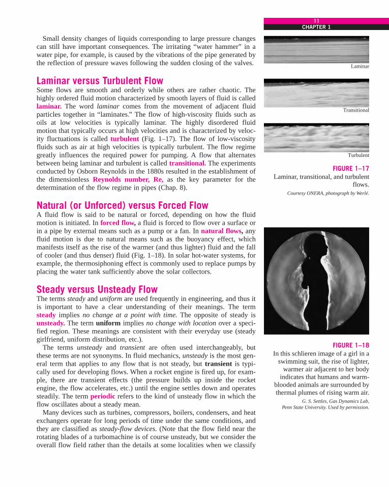
Natural (or Unforced) versus Forced FlowA fluid flow is said to be natural or forced, depending on how the fluidmotion is initiated. In forced flow, a fluid is forced to flow over a surface orin a pipe by external means such as a pump or a fan. In natural flows, anyfluid motion is due to natural means such as the buoyancy effect, whichmanifests itself as the rise of the warmer (and thus lighter) fluid and the fallof cooler (and thus denser) fluid (Fig. 1–18). In solar hot-water systems, forexample, the thermosiphoning effect is commonly used to replace pumps byplacing the water tank sufficiently above the solar collectors.

Steady versus Unsteady FlowThe terms steady and uniform are used frequently in engineering, and thus itis important to have a clear understanding of their meanings. The termsteady implies no change at a point with time. The opposite of steady isunsteady. The term uniform implies no change with location over a speci-fied region. These meanings are consistent with their everyday use (steadygirlfriend, uniform distribution, etc.).

The terms unsteady and transient are often used interchangeably, butthese terms are not synonyms. In fluid mechanics, unsteady is the most gen-eral term that applies to any flow that is not steady, but transient is typi-cally used for developing flows. When a rocket engine is fired up, for exam-ple, there are transient effects (the pressure builds up inside the rocketengine, the flow accelerates, etc.) until the engine settles down and operatessteadily. The term periodic refers to the kind of unsteady flow in which theflow oscillates about a steady mean.

Many devices such as turbines, compressors, boilers, condensers, and heatexchangers operate for long periods of time under the same conditions, andthey are classified as steady-flow devices. (Note that the flow field near therotating blades of a turbomachine is of course unsteady, but we consider theoverall flow field rather than the details at some localities when we classify

11CHAPTER 1

Laminar

Transitional

Turbulent

FIGURE 1–17Laminar, transitional, and turbulent

flows.Courtesy ONERA, photograph by Werlé.

FIGURE 1–18In this schlieren image of a girl in a

swimming suit, the rise of lighter,warmer air adjacent to her body

indicates that humans and warm-blooded animals are surrounded bythermal plumes of rising warm air.

G. S. Settles, Gas Dynamics Lab,Penn State University. Used by permission.

cen72367_ch01.qxd 10/29/04 2:32 PM Page 11

devices.) During steady flow, the fluid properties can change from point topoint within a device, but at any fixed point they remain constant. There-fore, the volume, the mass, and the total energy content of a steady-flowdevice or flow section remain constant in steady operation.

Steady-flow conditions can be closely approximated by devices that areintended for continuous operation such as turbines, pumps, boilers, con-densers, and heat exchangers of power plants or refrigeration systems. Somecyclic devices, such as reciprocating engines or compressors, do not satisfythe steady-flow conditions since the flow at the inlets and the exits is pulsat-ing and not steady. However, the fluid properties vary with time in a peri-odic manner, and the flow through these devices can still be analyzed as asteady-flow process by using time-averaged values for the properties.

Some fascinating visualizations of fluid flow are provided in the book AnAlbum of Fluid Motion by Milton Van Dyke (1982). A nice illustration of anunsteady-flow field is shown in Fig. 1–19, taken from Van Dyke’s book.Figure 1–19a is an instantaneous snapshot from a high-speed motion pic-ture; it reveals large, alternating, swirling, turbulent eddies that are shed intothe periodically oscillating wake from the blunt base of the object. Theeddies produce shock waves that move upstream alternately over the top andbottom surfaces of the airfoil in an unsteady fashion. Figure 1–19b showsthe same flow field, but the film is exposed for a longer time so that theimage is time averaged over 12 cycles. The resulting time-averaged flowfield appears “steady” since the details of the unsteady oscillations havebeen lost in the long exposure.

One of the most important jobs of an engineer is to determine whether itis sufficient to study only the time-averaged “steady” flow features of aproblem, or whether a more detailed study of the unsteady features isrequired. If the engineer were interested only in the overall properties of theflow field, (such as the time-averaged drag coefficient, the mean velocity,and pressure fields) a time-averaged description like that of Fig. 1–19b,time-averaged experimental measurements, or an analytical or numericalcalculation of the time-averaged flow field would be sufficient. However, ifthe engineer were interested in details about the unsteady-flow field, such asflow-induced vibrations, unsteady pressure fluctuations, or the sound wavesemitted from the turbulent eddies or the shock waves, a time-averageddescription of the flow field would be insufficient.

Most of the analytical and computational examples provided in this text-book deal with steady or time-averaged flows, although we occasionallypoint out some relevant unsteady-flow features as well when appropriate.

One-, Two-, and Three-Dimensional FlowsA flow field is best characterized by the velocity distribution, and thus aflow is said to be one-, two-, or three-dimensional if the flow velocity variesin one, two, or three primary dimensions, respectively. A typical fluid flowinvolves a three-dimensional geometry, and the velocity may vary in allthree dimensions, rendering the flow three-dimensional [V

!

(x, y, z) in rec-tangular or V

!

(r, u, z) in cylindrical coordinates]. However, the variation ofvelocity in certain directions can be small relative to the variation in otherdirections and can be ignored with negligible error. In such cases, the flowcan be modeled conveniently as being one- or two-dimensional, which iseasier to analyze.

12FLUID MECHANICS

(a)

(b)

FIGURE 1–19Oscillating wake of a blunt-basedairfoil at Mach number 0.6. Photo (a)is an instantaneous image, whilephoto (b) is a long-exposure (time-averaged) image.(a) Dyment, A., Flodrops, J. P. & Gryson, P. 1982in Flow Visualization II, W. Merzkirch, ed.,331–336. Washington: Hemisphere. Used bypermission of Arthur Dyment.

(b) Dyment, A. & Gryson, P. 1978 in Inst. Mèc.Fluides Lille, No. 78-5. Used by permission ofArthur Dyment.

cen72367_ch01.qxd 10/29/04 2:32 PM Page 12

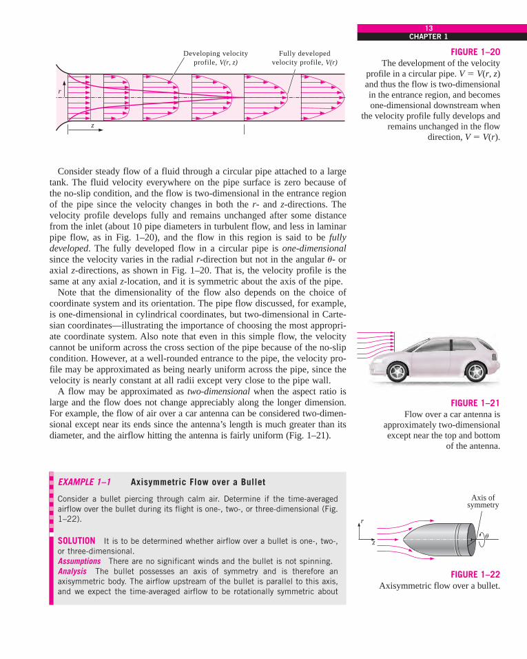
Consider steady flow of a fluid through a circular pipe attached to a largetank. The fluid velocity everywhere on the pipe surface is zero because ofthe no-slip condition, and the flow is two-dimensional in the entrance regionof the pipe since the velocity changes in both the r- and z-directions. Thevelocity profile develops fully and remains unchanged after some distancefrom the inlet (about 10 pipe diameters in turbulent flow, and less in laminarpipe flow, as in Fig. 1–20), and the flow in this region is said to be fullydeveloped. The fully developed flow in a circular pipe is one-dimensionalsince the velocity varies in the radial r-direction but not in the angular u- oraxial z-directions, as shown in Fig. 1–20. That is, the velocity profile is thesame at any axial z-location, and it is symmetric about the axis of the pipe.

Note that the dimensionality of the flow also depends on the choice ofcoordinate system and its orientation. The pipe flow discussed, for example,is one-dimensional in cylindrical coordinates, but two-dimensional in Carte-sian coordinates—illustrating the importance of choosing the most appropri-ate coordinate system. Also note that even in this simple flow, the velocitycannot be uniform across the cross section of the pipe because of the no-slipcondition. However, at a well-rounded entrance to the pipe, the velocity pro-file may be approximated as being nearly uniform across the pipe, since thevelocity is nearly constant at all radii except very close to the pipe wall.

A flow may be approximated as two-dimensional when the aspect ratio islarge and the flow does not change appreciably along the longer dimension.For example, the flow of air over a car antenna can be considered two-dimen-sional except near its ends since the antenna’s length is much greater than itsdiameter, and the airflow hitting the antenna is fairly uniform (Fig. 1–21).

EXAMPLE 1–1 Axisymmetric Flow over a Bullet

Consider a bullet piercing through calm air. Determine if the time-averagedairflow over the bullet during its flight is one-, two-, or three-dimensional (Fig.1–22).

SOLUTION It is to be determined whether airflow over a bullet is one-, two-,or three-dimensional.Assumptions There are no significant winds and the bullet is not spinning.Analysis The bullet possesses an axis of symmetry and is therefore anaxisymmetric body. The airflow upstream of the bullet is parallel to this axis,and we expect the time-averaged airflow to be rotationally symmetric about

13CHAPTER 1

z

r

Developing velocityprofile, V(r, z)

Fully developedvelocity profile, V(r)

FIGURE 1–20The development of the velocity

profile in a circular pipe. V ! V(r, z)and thus the flow is two-dimensionalin the entrance region, and becomesone-dimensional downstream when

the velocity profile fully develops andremains unchanged in the flow

direction, V ! V(r).

FIGURE 1–21Flow over a car antenna is

approximately two-dimensional except near the top and bottom

of the antenna.

Axis ofsymmetry

r

zu

FIGURE 1–22Axisymmetric flow over a bullet.

cen72367_ch01.qxd 10/29/04 2:32 PM Page 13

the axis—such flows are said to be axisymmetric. The velocity in this casevaries with axial distance z and radial distance r, but not with angle u.Therefore, the time-averaged airflow over the bullet is two-dimensional.Discussion While the time-averaged airflow is axisymmetric, the instanta-neous airflow is not, as illustrated in Fig. 1–19.

1–5 ! SYSTEM AND CONTROL VOLUMEA system is defined as a quantity of matter or a region in space chosen forstudy. The mass or region outside the system is called the surroundings.The real or imaginary surface that separates the system from its surround-ings is called the boundary (Fig. 1–23). The boundary of a system can befixed or movable. Note that the boundary is the contact surface shared byboth the system and the surroundings. Mathematically speaking, the bound-ary has zero thickness, and thus it can neither contain any mass nor occupyany volume in space.

Systems may be considered to be closed or open, depending on whether afixed mass or a volume in space is chosen for study. A closed system (alsoknown as a control mass) consists of a fixed amount of mass, and no masscan cross its boundary. But energy, in the form of heat or work, can crossthe boundary, and the volume of a closed system does not have to be fixed.If, as a special case, even energy is not allowed to cross the boundary, thatsystem is called an isolated system.

Consider the piston–cylinder device shown in Fig. 1–24. Let us say thatwe would like to find out what happens to the enclosed gas when it isheated. Since we are focusing our attention on the gas, it is our system. Theinner surfaces of the piston and the cylinder form the boundary, and sinceno mass is crossing this boundary, it is a closed system. Notice that energymay cross the boundary, and part of the boundary (the inner surface of thepiston, in this case) may move. Everything outside the gas, including thepiston and the cylinder, is the surroundings.

An open system, or a control volume, as it is often called, is a properlyselected region in space. It usually encloses a device that involves mass flowsuch as a compressor, turbine, or nozzle. Flow through these devices is beststudied by selecting the region within the device as the control volume.Both mass and energy can cross the boundary of a control volume.

A large number of engineering problems involve mass flow in and out ofa system and, therefore, are modeled as control volumes. A water heater, acar radiator, a turbine, and a compressor all involve mass flow and shouldbe analyzed as control volumes (open systems) instead of as control masses(closed systems). In general, any arbitrary region in space can be selectedas a control volume. There are no concrete rules for the selection of controlvolumes, but the proper choice certainly makes the analysis much easier. Ifwe were to analyze the flow of air through a nozzle, for example, a goodchoice for the control volume would be the region within the nozzle.

A control volume can be fixed in size and shape, as in the case of a noz-zle, or it may involve a moving boundary, as shown in Fig. 1–25. Most con-trol volumes, however, have fixed boundaries and thus do not involve any

14FLUID MECHANICS

SURROUNDINGS

BOUNDARY

SYSTEM

FIGURE 1–23System, surroundings, and boundary.

GAS2 kg1.5 m3GAS

2 kg1 m3

Movingboundary

Fixedboundary

FIGURE 1–24A closed system with a movingboundary.

cen72367_ch01.qxd 10/29/04 2:32 PM Page 14

moving boundaries. A control volume may also involve heat and work inter-actions just as a closed system, in addition to mass interaction.

1–6 ! IMPORTANCE OF DIMENSIONS AND UNITSAny physical quantity can be characterized by dimensions. The magnitudesassigned to the dimensions are called units. Some basic dimensions such asmass m, length L, time t, and temperature T are selected as primary or fun-damental dimensions, while others such as velocity V, energy E, and vol-ume V are expressed in terms of the primary dimensions and are called sec-ondary dimensions, or derived dimensions.

A number of unit systems have been developed over the years. Despitestrong efforts in the scientific and engineering community to unify theworld with a single unit system, two sets of units are still in common usetoday: the English system, which is also known as the United States Cus-tomary System (USCS), and the metric SI (from Le Système Internationald’ Unités), which is also known as the International System. The SI is a sim-ple and logical system based on a decimal relationship between the variousunits, and it is being used for scientific and engineering work in most of theindustrialized nations, including England. The English system, however, hasno apparent systematic numerical base, and various units in this system arerelated to each other rather arbitrarily (12 in ! 1 ft, 1 mile ! 5280 ft, 4 qt! 1 gal, etc.), which makes it confusing and difficult to learn. The UnitedStates is the only industrialized country that has not yet fully converted tothe metric system.

The systematic efforts to develop a universally acceptable system of unitsdates back to 1790 when the French National Assembly charged the FrenchAcademy of Sciences to come up with such a unit system. An early versionof the metric system was soon developed in France, but it did not find uni-versal acceptance until 1875 when The Metric Convention Treaty was pre-pared and signed by 17 nations, including the United States. In this interna-tional treaty, meter and gram were established as the metric units for lengthand mass, respectively, and a General Conference of Weights and Measures(CGPM) was established that was to meet every six years. In 1960, the

15CHAPTER 1

CV

Movingboundary

Fixedboundary

CV(a nozzle)

Real boundary

(b) A control volume (CV) with fixed and moving boundaries

(a) A control volume (CV) with real and imaginary boundaries

Imaginaryboundary

FIGURE 1–25A control volume may involve fixed,

moving, real, and imaginaryboundaries.

cen72367_ch01.qxd 10/29/04 2:32 PM Page 15

CGPM produced the SI, which was based on six fundamental quantities,and their units were adopted in 1954 at the Tenth General Conference ofWeights and Measures: meter (m) for length, kilogram (kg) for mass, sec-ond (s) for time, ampere (A) for electric current, degree Kelvin (°K) fortemperature, and candela (cd) for luminous intensity (amount of light). In1971, the CGPM added a seventh fundamental quantity and unit: mole(mol) for the amount of matter.

Based on the notational scheme introduced in 1967, the degree symbolwas officially dropped from the absolute temperature unit, and all unitnames were to be written without capitalization even if they were derivedfrom proper names (Table 1–1). However, the abbreviation of a unit was tobe capitalized if the unit was derived from a proper name. For example, theSI unit of force, which is named after Sir Isaac Newton (1647–1723), isnewton (not Newton), and it is abbreviated as N. Also, the full name of aunit may be pluralized, but its abbreviation cannot. For example, the lengthof an object can be 5 m or 5 meters, not 5 ms or 5 meter. Finally, no periodis to be used in unit abbreviations unless they appear at the end of a sen-tence. For example, the proper abbreviation of meter is m (not m.).

The recent move toward the metric system in the United States seems tohave started in 1968 when Congress, in response to what was happening inthe rest of the world, passed a Metric Study Act. Congress continued to pro-mote a voluntary switch to the metric system by passing the Metric Conver-sion Act in 1975. A trade bill passed by Congress in 1988 set a September1992 deadline for all federal agencies to convert to the metric system. How-ever, the deadlines were relaxed later with no clear plans for the future.

The industries that are heavily involved in international trade (such as theautomotive, soft drink, and liquor industries) have been quick in convertingto the metric system for economic reasons (having a single worldwidedesign, fewer sizes, smaller inventories, etc.). Today, nearly all the carsmanufactured in the United States are metric. Most car owners probably donot realize this until they try an English socket wrench on a metric bolt.Most industries, however, resisted the change, thus slowing down the con-version process.

Presently the United States is a dual-system society, and it will stay thatway until the transition to the metric system is completed. This puts an extraburden on today’s engineering students, since they are expected to retaintheir understanding of the English system while learning, thinking, andworking in terms of the SI. Given the position of the engineers in the transi-tion period, both unit systems are used in this text, with particular emphasison SI units.

As pointed out, the SI is based on a decimal relationship between units.The prefixes used to express the multiples of the various units are listed inTable 1–2. They are standard for all units, and the student is encouraged tomemorize them because of their widespread use (Fig. 1–26).

Some SI and English UnitsIn SI, the units of mass, length, and time are the kilogram (kg), meter (m),and second (s), respectively. The respective units in the English system arethe pound-mass (lbm), foot (ft), and second (s). The pound symbol lb is

16FLUID MECHANICS

TABLE 1–1The seven fundamental (or primary)dimensions and their units in SI

Dimension Unit

Length meter (m)Mass kilogram (kg)Time second (s)Temperature kelvin (K)Electric current ampere (A)Amount of light candela (cd)Amount of matter mole (mol)

TABLE 1–2Standard prefixes in SI units

Multiple Prefix

1012 tera, T109 giga, G106 mega, M103 kilo, k102 hecto, h101 deka, da10$1 deci, d10$2 centi, c10$3 milli, m10$6 micro, m10$9 nano, n10$12 pico, p

cen72367_ch01.qxd 10/29/04 2:32 PM Page 16

actually the abbreviation of libra, which was the ancient Roman unit ofweight. The English retained this symbol even after the end of the Romanoccupation of Britain in 410. The mass and length units in the two systemsare related to each other by

In the English system, force is usually considered to be one of the pri-mary dimensions and is assigned a nonderived unit. This is a source of con-fusion and error that necessitates the use of a dimensional constant (gc) inmany formulas. To avoid this nuisance, we consider force to be a secondarydimension whose unit is derived from Newton’s second law, i.e.,

Force ! (Mass) (Acceleration)

or F ! ma (1–1)

In SI, the force unit is the newton (N), and it is defined as the force requiredto accelerate a mass of 1 kg at a rate of 1 m/s2. In the English system, theforce unit is the pound-force (lbf) and is defined as the force required toaccelerate a mass of 32.174 lbm (1 slug) at a rate of 1 ft/s2 (Fig. 1–27).That is,

A force of 1 N is roughly equivalent to the weight of a small apple (m! 102 g), whereas a force of 1 lbf is roughly equivalent to the weight offour medium apples (mtotal ! 454 g), as shown in Fig. 1–28. Another forceunit in common use in many European countries is the kilogram-force (kgf),which is the weight of 1 kg mass at sea level (1 kgf ! 9.807 N).

The term weight is often incorrectly used to express mass, particularly bythe “weight watchers.” Unlike mass, weight W is a force. It is the gravita-tional force applied to a body, and its magnitude is determined from New-ton’s second law,

(1–2)

where m is the mass of the body, and g is the local gravitational acceleration(g is 9.807 m/s2 or 32.174 ft/s2 at sea level and 45° latitude). An ordinarybathroom scale measures the gravitational force acting on a body. Theweight of a unit volume of a substance is called the specific weight g and isdetermined from g ! rg, where r is density.

The mass of a body remains the same regardless of its location in the uni-verse. Its weight, however, changes with a change in gravitational accelera-tion. A body weighs less on top of a mountain since g decreases with altitude.

W ! mg (N)

1 lbf ! 32.174 lbm " ft/s2

1 N ! 1 kg " m/s2

1 ft ! 0.3048 m

1 lbm ! 0.45359 kg

17CHAPTER 1

200 mL(0.2 L)

1 kg(103 g)

1 M#

(106 #)

FIGURE 1–26The SI unit prefixes are used in all

branches of engineering.

m = 1 kg

m = 32.174 lbm

a = 1 m/s 2

a = 1 ft/s 2

F = 1 lbf

F = 1 N

FIGURE 1–27The definition of the force units.

1 kgf

10 applesm = 1 kg

4 applesm = 1 lbm

1 lbf

1 applem = 102 g

1 N

FIGURE 1–28The relative magnitudes of the force

units newton (N), kilogram-force(kgf), and pound-force (lbf).

cen72367_ch01.qxd 11/17/04 2:12 PM Page 17

On the surface of the moon, an astronaut weighs about one-sixth of whatshe or he normally weighs on earth (Fig. 1–29).

At sea level a mass of 1 kg weighs 9.807 N, as illustrated in Fig. 1–30. Amass of 1 lbm, however, weighs 1 lbf, which misleads people to believe thatpound-mass and pound-force can be used interchangeably as pound (lb),which is a major source of error in the English system.

It should be noted that the gravity force acting on a mass is due to theattraction between the masses, and thus it is proportional to the magnitudesof the masses and inversely proportional to the square of the distancebetween them. Therefore, the gravitational acceleration g at a locationdepends on the local density of the earth’s crust, the distance to the centerof the earth, and to a lesser extent, the positions of the moon and the sun.The value of g varies with location from 9.8295 m/s2 at 4500 m below sealevel to 7.3218 m/s2 at 100,000 m above sea level. However, at altitudes upto 30,000 m, the variation of g from the sea-level value of 9.807 m/s2 is lessthan 1 percent. Therefore, for most practical purposes, the gravitationalacceleration can be assumed to be constant at 9.81 m/s2. It is interesting tonote that at locations below sea level, the value of g increases with distancefrom the sea level, reaches a maximum at about 4500 m, and then startsdecreasing. (What do you think the value of g is at the center of the earth?)

The primary cause of confusion between mass and weight is that mass isusually measured indirectly by measuring the gravity force it exerts. Thisapproach also assumes that the forces exerted by other effects such as airbuoyancy and fluid motion are negligible. This is like measuring the dis-tance to a star by measuring its red shift, or measuring the altitude of an air-plane by measuring barometric pressure. Both of these are also indirectmeasurements. The correct direct way of measuring mass is to compare it toa known mass. This is cumbersome, however, and it is mostly used for cali-bration and measuring precious metals.

Work, which is a form of energy, can simply be defined as force times dis-tance; therefore, it has the unit “newton-meter (N . m),” which is called ajoule (J). That is,

(1–3)

A more common unit for energy in SI is the kilojoule (1 kJ ! 103 J). In theEnglish system, the energy unit is the Btu (British thermal unit), which isdefined as the energy required to raise the temperature of 1 lbm of water at68°F by 1°F. In the metric system, the amount of energy needed to raise thetemperature of 1 g of water at 14.5°C by 1°C is defined as 1 calorie (cal),and 1 cal ! 4.1868 J. The magnitudes of the kilojoule and Btu are almostidentical (1 Btu ! 1.0551 kJ).

Dimensional HomogeneityWe all know from grade school that apples and oranges do not add. But wesomehow manage to do it (by mistake, of course). In engineering, all equa-tions must be dimensionally homogeneous. That is, every term in an equa-tion must have the same unit (Fig. 1–31). If, at some stage of an analysis,we find ourselves in a position to add two quantities that have differentunits, it is a clear indication that we have made an error at an earlier stage.So checking dimensions can serve as a valuable tool to spot errors.

1 J ! 1 N % m

18FLUID MECHANICS

FIGURE 1–29A body weighing 150 lbf on earth willweigh only 25 lbf on the moon.

g = 9.807 m/s2

W = 9.807 kg · m/s2

= 9.807 N = 1 kgf

W = 32.174 lbm · ft/s2

= 1 lbf

g = 32.174 ft/s2

kg lbm

FIGURE 1–30The weight of a unit mass at sea level.

FIGURE 1–31To be dimensionally homogeneous, allthe terms in an equation must have thesame unit.© Reprinted with special permission of KingFeatures Syndicate.

cen72367_ch01.qxd 10/29/04 2:32 PM Page 18

EXAMPLE 1–2 Spotting Errors from Unit Inconsistencies

While solving a problem, a person ended up with the following equation atsome stage:

where E is the total energy and has the unit of kilojoules. Determine how tocorrect the error and discuss what may have caused it.

SOLUTION During an analysis, a relation with inconsistent units is obtained.A correction is to be found, and the probable cause of the error is to bedetermined.Analysis The two terms on the right-hand side do not have the same units,and therefore they cannot be added to obtain the total energy. Multiplyingthe last term by mass will eliminate the kilograms in the denominator, andthe whole equation will become dimensionally homogeneous; that is, everyterm in the equation will have the same unit. Discussion Obviously this error was caused by forgetting to multiply the lastterm by mass at an earlier stage.

We all know from experience that units can give terrible headaches if theyare not used carefully in solving a problem. However, with some attentionand skill, units can be used to our advantage. They can be used to check for-mulas; they can even be used to derive formulas, as explained in the follow-ing example.

EXAMPLE 1–3 Obtaining Formulas from Unit Considerations

A tank is filled with oil whose density is r ! 850 kg/m3. If the volume of thetank is V ! 2 m3, determine the amount of mass m in the tank.

SOLUTION The volume of an oil tank is given. The mass of oil is to bedetermined.Assumptions Oil is an incompressible substance and thus its density isconstant.Analysis A sketch of the system just described is given in Fig. 1–32. Sup-pose we forgot the formula that relates mass to density and volume. However,we know that mass has the unit of kilograms. That is, whatever calculationswe do, we should end up with the unit of kilograms. Putting the given infor-mation into perspective, we have

It is obvious that we can eliminate m3 and end up with kg by multiplyingthese two quantities. Therefore, the formula we are looking for should be

Thus,

Discussion Note that this approach may not work for more complicatedformulas.

m ! (850 kg/m3)(2 m3) ! 1700 kg

m ! rV

r ! 850 kg/m3 and V ! 2 m3

E ! 25 kJ & 7 kJ/kg

19CHAPTER 1

V = 2 m3

" = 850 kg/m3

m = ?

OIL

FIGURE 1–32Schematic for Example 1–3.

cen72367_ch01.qxd 10/29/04 2:32 PM Page 19

20FLUID MECHANICS

lbm

FIGURE 1–33A mass of 1 lbm weighs 1 lbf on earth.

The student should keep in mind that a formula that is not dimensionallyhomogeneous is definitely wrong, but a dimensionally homogeneous for-mula is not necessarily right.

Unity Conversion RatiosJust as all nonprimary dimensions can be formed by suitable combinationsof primary dimensions, all nonprimary units (secondary units) can beformed by combinations of primary units. Force units, for example, can beexpressed as

They can also be expressed more conveniently as unity conversion ratios as

Unity conversion ratios are identically equal to 1 and are unitless, and thussuch ratios (or their inverses) can be inserted conveniently into any calcula-tion to properly convert units. Students are encouraged to always use unityconversion ratios such as those given here when converting units. Some text-books insert the archaic gravitational constant gc defined as gc ! 32.174 lbm· ft/lbf · s2 ! kg · m/N · s2 ! 1 into equations in order to force units tomatch. This practice leads to unnecessary confusion and is strongly discour-aged by the present authors. We recommend that students instead use unityconversion ratios.

EXAMPLE 1–4 The Weight of One Pound-Mass

Using unity conversion ratios, show that 1.00 lbm weighs 1.00 lbf on earth(Fig. 1–33).

Solution A mass of 1.00 lbm is subjected to standard earth gravity. Itsweight in lbf is to be determined.Assumptions Standard sea-level conditions are assumed.Properties The gravitational constant is g ! 32.174 ft/s2.Analysis We apply Newton’s second law to calculate the weight (force) thatcorresponds to the known mass and acceleration. The weight of any object isequal to its mass times the local value of gravitational acceleration. Thus,

Discussion Mass is the same regardless of its location. However, on someother planet with a different value of gravitational acceleration, the weight of1 lbm would differ from that calculated here.

When you buy a box of breakfast cereal, the printing may say “Netweight: One pound (454 grams).” (See Fig. 1–34.) Technically, this meansthat the cereal inside the box weighs 1.00 lbf on earth and has a mass of

W ! mg ! (1.00 lbm)(32.174 ft/s2)a 1 lbf32.174 lbm % ft/s2b ! 1.00 lbf

Nkg % m/s2 ! 1 and

lbf32.174 lbm % ft/s2 ! 1

N ! kg ms2 and lbf ! 32.174 lbm

fts2

cen72367_ch01.qxd 10/29/04 2:32 PM Page 20

453.6 gm (0.4536 kg). Using Newton’s second law, the actual weight onearth of the cereal in the metric system is

1–7 ! MATHEMATICAL MODELING OF ENGINEERING PROBLEMS

An engineering device or process can be studied either experimentally (test-ing and taking measurements) or analytically (by analysis or calculations).The experimental approach has the advantage that we deal with the actualphysical system, and the desired quantity is determined by measurement,within the limits of experimental error. However, this approach is expensive,time-consuming, and often impractical. Besides, the system we are studyingmay not even exist. For example, the entire heating and plumbing systemsof a building must usually be sized before the building is actually built onthe basis of the specifications given. The analytical approach (including thenumerical approach) has the advantage that it is fast and inexpensive, butthe results obtained are subject to the accuracy of the assumptions, approxi-mations, and idealizations made in the analysis. In engineering studies,often a good compromise is reached by reducing the choices to just a fewby analysis, and then verifying the findings experimentally.

Modeling in EngineeringThe descriptions of most scientific problems involve equations that relatethe changes in some key variables to each other. Usually the smaller theincrement chosen in the changing variables, the more general and accuratethe description. In the limiting case of infinitesimal or differential changesin variables, we obtain differential equations that provide precise mathemat-ical formulations for the physical principles and laws by representing therates of change as derivatives. Therefore, differential equations are used toinvestigate a wide variety of problems in sciences and engineering (Fig.1–35). However, many problems encountered in practice can be solvedwithout resorting to differential equations and the complications associatedwith them.

The study of physical phenomena involves two important steps. In thefirst step, all the variables that affect the phenomena are identified, reason-able assumptions and approximations are made, and the interdependence ofthese variables is studied. The relevant physical laws and principles areinvoked, and the problem is formulated mathematically. The equation itselfis very instructive as it shows the degree of dependence of some variableson others, and the relative importance of various terms. In the second step,the problem is solved using an appropriate approach, and the results areinterpreted.

Many processes that seem to occur in nature randomly and without anyorder are, in fact, being governed by some visible or not-so-visible physicallaws. Whether we notice them or not, these laws are there, governing con-sistently and predictably over what seem to be ordinary events. Most of

W ! mg ! (453.6 g)(9.81 m/s2)a 1 N1 kg % m/s2b a 1 kg

1000 gb ! 4.49 N

21CHAPTER 1

Net weight:One pound (454 grams)

FIGURE 1–34A quirk in the metric system of units.

Identifyimportantvariables Make

reasonableassumptions andapproximationsApply

relevantphysical laws

Physical problem

A differential equation

Applyapplicablesolution

technique

Applyboundaryand initialconditions

Solution of the problem

FIGURE 1–35Mathematical modeling of physical

problems.

cen72367_ch01.qxd 10/29/04 2:32 PM Page 21

these laws are well defined and well understood by scientists. This makes itpossible to predict the course of an event before it actually occurs or tostudy various aspects of an event mathematically without actually runningexpensive and time-consuming experiments. This is where the power ofanalysis lies. Very accurate results to meaningful practical problems can beobtained with relatively little effort by using a suitable and realistic mathe-matical model. The preparation of such models requires an adequate knowl-edge of the natural phenomena involved and the relevant laws, as well assound judgment. An unrealistic model will obviously give inaccurate andthus unacceptable results.

An analyst working on an engineering problem often finds himself or her-self in a position to make a choice between a very accurate but complexmodel, and a simple but not-so-accurate model. The right choice depends onthe situation at hand. The right choice is usually the simplest model thatyields satisfactory results. Also, it is important to consider the actual operat-ing conditions when selecting equipment.

Preparing very accurate but complex models is usually not so difficult.But such models are not much use to an analyst if they are very difficult andtime-consuming to solve. At the minimum, the model should reflect theessential features of the physical problem it represents. There are many sig-nificant real-world problems that can be analyzed with a simple model. Butit should always be kept in mind that the results obtained from an analysisare at best as accurate as the assumptions made in simplifying the problem.Therefore, the solution obtained should not be applied to situations forwhich the original assumptions do not hold.

A solution that is not quite consistent with the observed nature of the prob-lem indicates that the mathematical model used is too crude. In that case, amore realistic model should be prepared by eliminating one or more of thequestionable assumptions. This will result in a more complex problem that,of course, is more difficult to solve. Thus any solution to a problem shouldbe interpreted within the context of its formulation.

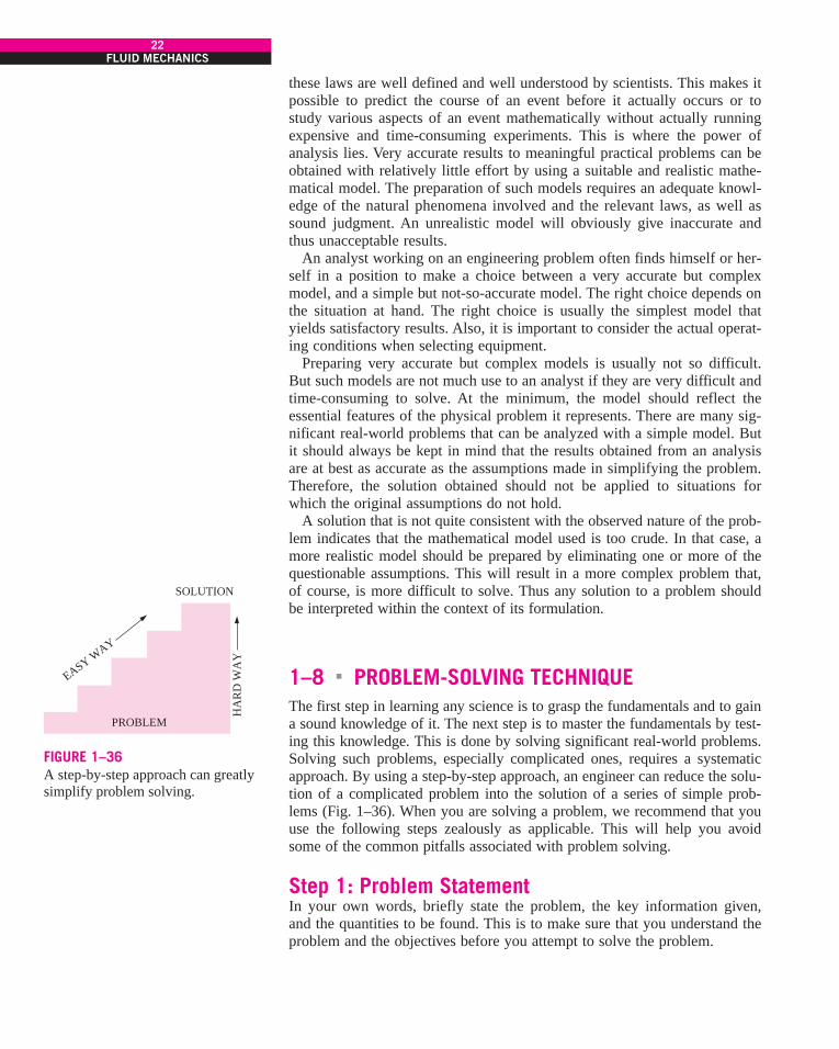
1–8 ! PROBLEM-SOLVING TECHNIQUEThe first step in learning any science is to grasp the fundamentals and to gaina sound knowledge of it. The next step is to master the fundamentals by test-ing this knowledge. This is done by solving significant real-world problems.Solving such problems, especially complicated ones, requires a systematicapproach. By using a step-by-step approach, an engineer can reduce the solu-tion of a complicated problem into the solution of a series of simple prob-lems (Fig. 1–36). When you are solving a problem, we recommend that youuse the following steps zealously as applicable. This will help you avoidsome of the common pitfalls associated with problem solving.

Step 1: Problem StatementIn your own words, briefly state the problem, the key information given,and the quantities to be found. This is to make sure that you understand theproblem and the objectives before you attempt to solve the problem.

22FLUID MECHANICS

SOLUTION

PROBLEM

HA

RD

WA

Y

EASY WAY

FIGURE 1–36A step-by-step approach can greatlysimplify problem solving.

cen72367_ch01.qxd 10/29/04 2:32 PM Page 22

Step 2: SchematicDraw a realistic sketch of the physical system involved, and list the relevantinformation on the figure. The sketch does not have to be something elabo-rate, but it should resemble the actual system and show the key features.Indicate any energy and mass interactions with the surroundings. Listing thegiven information on the sketch helps one to see the entire problem at once.Also, check for properties that remain constant during a process (such astemperature during an isothermal process), and indicate them on the sketch.

Step 3: Assumptions and ApproximationsState any appropriate assumptions and approximations made to simplify theproblem to make it possible to obtain a solution. Justify the questionableassumptions. Assume reasonable values for missing quantities that are nec-essary. For example, in the absence of specific data for atmospheric pres-sure, it can be taken to be 1 atm. However, it should be noted in the analysisthat the atmospheric pressure decreases with increasing elevation. For exam-ple, it drops to 0.83 atm in Denver (elevation 1610 m) (Fig. 1–37).

Step 4: Physical LawsApply all the relevant basic physical laws and principles (such as the con-servation of mass), and reduce them to their simplest form by utilizing theassumptions made. However, the region to which a physical law is appliedmust be clearly identified first. For example, the increase in speed of waterflowing through a nozzle is analyzed by applying conservation of massbetween the inlet and outlet of the nozzle.

Step 5: PropertiesDetermine the unknown properties at known states necessary to solve theproblem from property relations or tables. List the properties separately, andindicate their source, if applicable.

Step 6: CalculationsSubstitute the known quantities into the simplified relations and perform thecalculations to determine the unknowns. Pay particular attention to the unitsand unit cancellations, and remember that a dimensional quantity without aunit is meaningless. Also, don’t give a false implication of high precision bycopying all the digits from the screen of the calculator—round the results toan appropriate number of significant digits (Section 1–10).

Step 7: Reasoning, Verification, and DiscussionCheck to make sure that the results obtained are reasonable and intuitive,and verify the validity of the questionable assumptions. Repeat the calcula-tions that resulted in unreasonable values. For example, under the same testconditions the aerodynamic drag acting on a car should not increase afterstreamlining the shape of the car (Fig. 1–38).

Also, point out the significance of the results, and discuss their implica-tions. State the conclusions that can be drawn from the results, and any rec-ommendations that can be made from them. Emphasize the limitations

23CHAPTER 1

Given: Air temperature in Denver

To be found: Density of air

Missing information: Atmosphericpressure

Assumption #1: Take P = 1 atm(Inappropriate. Ignores effect of altitude. Will cause more than 15% error.)

Assumption #2: Take P = 0.83 atm(Appropriate. Ignores only minor effects such as weather.)

FIGURE 1–37The assumptions made while solving

an engineering problem must bereasonable and justifiable.

Before streamliningV

VAfter streamliningUnreasonable!

FD

FD

FIGURE 1–38The results obtained from an

engineering analysis must be checkedfor reasonableness.

cen72367_ch01.qxd 10/29/04 2:32 PM Page 23

under which the results are applicable, and caution against any possible mis-understandings and using the results in situations where the underlyingassumptions do not apply. For example, if you determined that using alarger-diameter pipe in a proposed pipeline will cost an additional $5000 inmaterials, but it will reduce the annual pumping costs by $3000, indicatethat the larger-diameter pipeline will pay for its cost differential from theelectricity it saves in less than two years. However, also state that only addi-tional material costs associated with the larger-diameter pipeline are consid-ered in the analysis.

Keep in mind that the solutions you present to your instructors, and anyengineering analysis presented to others, is a form of communication.Therefore neatness, organization, completeness, and visual appearance areof utmost importance for maximum effectiveness. Besides, neatness alsoserves as a great checking tool since it is very easy to spot errors and incon-sistencies in neat work. Carelessness and skipping steps to save time oftenend up costing more time and unnecessary anxiety.

The approach described here is used in the solved example problems with-out explicitly stating each step, as well as in the Solutions Manual of thistext. For some problems, some of the steps may not be applicable or neces-sary. For example, often it is not practical to list the properties separately.However, we cannot overemphasize the importance of a logical and orderlyapproach to problem solving. Most difficulties encountered while solving aproblem are not due to a lack of knowledge; rather, they are due to a lack oforganization. You are strongly encouraged to follow these steps in problemsolving until you develop your own approach that works best for you.

1–9 ! ENGINEERING SOFTWARE PACKAGESYou may be wondering why we are about to undertake an in-depth study ofthe fundamentals of another engineering science. After all, almost all suchproblems we are likely to encounter in practice can be solved using one ofseveral sophisticated software packages readily available in the markettoday. These software packages not only give the desired numerical results,but also supply the outputs in colorful graphical form for impressive presen-tations. It is unthinkable to practice engineering today without using someof these packages. This tremendous computing power available to us at thetouch of a button is both a blessing and a curse. It certainly enables engi-neers to solve problems easily and quickly, but it also opens the door forabuses and misinformation. In the hands of poorly educated people, thesesoftware packages are as dangerous as sophisticated powerful weapons inthe hands of poorly trained soldiers.

Thinking that a person who can use the engineering software packageswithout proper training on fundamentals can practice engineering is likethinking that a person who can use a wrench can work as a car mechanic. Ifit were true that the engineering students do not need all these fundamentalcourses they are taking because practically everything can be done by com-puters quickly and easily, then it would also be true that the employers wouldno longer need high-salaried engineers since any person who knows how touse a word-processing program can also learn how to use those softwarepackages. However, the statistics show that the need for engineers is on therise, not on the decline, despite the availability of these powerful packages.

24FLUID MECHANICS

cen72367_ch01.qxd 10/29/04 2:32 PM Page 24

We should always remember that all the computing power and the engi-neering software packages available today are just tools, and tools havemeaning only in the hands of masters. Having the best word-processing pro-gram does not make a person a good writer, but it certainly makes the job ofa good writer much easier and makes the writer more productive (Fig.1–39). Hand calculators did not eliminate the need to teach our childrenhow to add or subtract, and the sophisticated medical software packages didnot take the place of medical school training. Neither will engineering soft-ware packages replace the traditional engineering education. They will sim-ply cause a shift in emphasis in the courses from mathematics to physics.That is, more time will be spent in the classroom discussing the physicalaspects of the problems in greater detail, and less time on the mechanics ofsolution procedures.

All these marvelous and powerful tools available today put an extra bur-den on today’s engineers. They must still have a thorough understanding ofthe fundamentals, develop a “feel” of the physical phenomena, be able toput the data into proper perspective, and make sound engineering judg-ments, just like their predecessors. However, they must do it much better,and much faster, using more realistic models because of the powerful toolsavailable today. The engineers in the past had to rely on hand calculations,slide rules, and later hand calculators and computers. Today they rely onsoftware packages. The easy access to such power and the possibility of asimple misunderstanding or misinterpretation causing great damage make itmore important today than ever to have solid training in the fundamentals ofengineering. In this text we make an extra effort to put the emphasis ondeveloping an intuitive and physical understanding of natural phenomenainstead of on the mathematical details of solution procedures.

Engineering Equation Solver (EES)EES is a program that solves systems of linear or nonlinear algebraic or dif-ferential equations numerically. It has a large library of built-in thermody-namic property functions as well as mathematical functions, and allows theuser to supply additional property data. Unlike some software packages,EES does not solve engineering problems; it only solves the equations sup-plied by the user. Therefore, the user must understand the problem and for-mulate it by applying any relevant physical laws and relations. EES savesthe user considerable time and effort by simply solving the resulting mathe-matical equations. This makes it possible to attempt significant engineeringproblems not suitable for hand calculations and to conduct parametric stud-ies quickly and conveniently. EES is a very powerful yet intuitive programthat is very easy to use, as shown in Example 1–5. The use and capabilitiesof EES are explained in Appendix 3 on the enclosed DVD.

EXAMPLE 1–5 Solving a System of Equations with EES

The difference of two numbers is 4, and the sum of the squares of these twonumbers is equal to the sum of the numbers plus 20. Determine these twonumbers.

25CHAPTER 1

Attached is a pdf of the text with windows and approx sizes for the art.

I'll give you rough ideas on the art, though you may have some differentthoughts on approaching these.

Fig 1 - 41 x 30The boxes fall into 2 columns, Type 1/2 on left and Type 1 on right.Nonenzymatic glycation is in the middle, between columns. Oxidative Stressand Axonal Degeneration are common outcomes and should be centered at thebottom beneath both columns (no need to stack them as shown). I wish I knewwhat the Polyol Pathway was, cause I'd like to illustrate it somehow.

Fig 2 -- 41 x 26This one's kinda straighforward, though I'd push Type 1/2 and Hyperglycemiafurther to the left, so that everything falls roughly under the other, Type1 column.

FIGURE 1–39An excellent word-processing

program does not make a person a good writer; it simply makes a

good writer a more efficient writer.

cen72367_ch01.qxd 10/29/04 2:32 PM Page 25

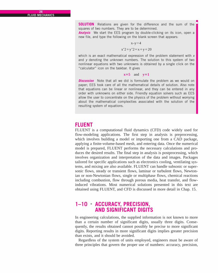
SOLUTION Relations are given for the difference and the sum of thesquares of two numbers. They are to be determined.Analysis We start the EES program by double-clicking on its icon, open anew file, and type the following on the blank screen that appears:

which is an exact mathematical expression of the problem statement with xand y denoting the unknown numbers. The solution to this system of twononlinear equations with two unknowns is obtained by a single click on the“calculator” icon on the taskbar. It gives

Discussion Note that all we did is formulate the problem as we would onpaper; EES took care of all the mathematical details of solution. Also notethat equations can be linear or nonlinear, and they can be entered in anyorder with unknowns on either side. Friendly equation solvers such as EESallow the user to concentrate on the physics of the problem without worryingabout the mathematical complexities associated with the solution of theresulting system of equations.

FLUENTFLUENT is a computational fluid dynamics (CFD) code widely used forflow-modeling applications. The first step in analysis is preprocessing,which involves building a model or importing one from a CAD package,applying a finite-volume-based mesh, and entering data. Once the numericalmodel is prepared, FLUENT performs the necessary calculations and pro-duces the desired results. The final step in analysis is postprocessing, whichinvolves organization and interpretation of the data and images. Packagestailored for specific applications such as electronics cooling, ventilating sys-tems, and mixing are also available. FLUENT can handle subsonic or super-sonic flows, steady or transient flows, laminar or turbulent flows, Newton-ian or non-Newtonian flows, single or multiphase flows, chemical reactionsincluding combustion, flow through porous media, heat transfer, and flow-induced vibrations. Most numerical solutions presented in this text areobtained using FLUENT, and CFD is discussed in more detail in Chap. 15.

1–10 ! ACCURACY, PRECISION, AND SIGNIFICANT DIGITS

In engineering calculations, the supplied information is not known to morethan a certain number of significant digits, usually three digits. Conse-quently, the results obtained cannot possibly be precise to more significantdigits. Reporting results in more significant digits implies greater precisionthan exists, and it should be avoided.

Regardless of the system of units employed, engineers must be aware ofthree principles that govern the proper use of numbers: accuracy, precision,

x!5 and y!1

xˆ2&yˆ2!x&y&20

x–y!4

26FLUID MECHANICS

cen72367_ch01.qxd 10/29/04 2:32 PM Page 26

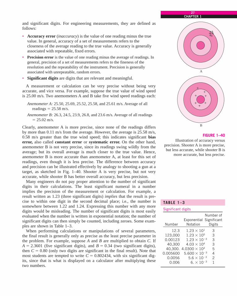
and significant digits. For engineering measurements, they are defined asfollows:

• Accuracy error (inaccuracy) is the value of one reading minus the truevalue. In general, accuracy of a set of measurements refers to thecloseness of the average reading to the true value. Accuracy is generallyassociated with repeatable, fixed errors.

• Precision error is the value of one reading minus the average of readings. Ingeneral, precision of a set of measurements refers to the fineness of theresolution and the repeatability of the instrument. Precision is generallyassociated with unrepeatable, random errors.

• Significant digits are digits that are relevant and meaningful.

A measurement or calculation can be very precise without being veryaccurate, and vice versa. For example, suppose the true value of wind speedis 25.00 m/s. Two anemometers A and B take five wind speed readings each:

Anemometer A: 25.50, 25.69, 25.52, 25.58, and 25.61 m/s. Average of allreadings ! 25.58 m/s.

Anemometer B: 26.3, 24.5, 23.9, 26.8, and 23.6 m/s. Average of all readings! 25.02 m/s.

Clearly, anemometer A is more precise, since none of the readings differsby more than 0.11 m/s from the average. However, the average is 25.58 m/s,0.58 m/s greater than the true wind speed; this indicates significant biaserror, also called constant error or systematic error. On the other hand,anemometer B is not very precise, since its readings swing wildly from theaverage; but its overall average is much closer to the true value. Hence,anemometer B is more accurate than anemometer A, at least for this set ofreadings, even though it is less precise. The difference between accuracyand precision can be illustrated effectively by analogy to shooting a gun at atarget, as sketched in Fig. 1–40. Shooter A is very precise, but not veryaccurate, while shooter B has better overall accuracy, but less precision.

Many engineers do not pay proper attention to the number of significantdigits in their calculations. The least significant numeral in a numberimplies the precision of the measurement or calculation. For example, aresult written as 1.23 (three significant digits) implies that the result is pre-cise to within one digit in the second decimal place; i.e., the number issomewhere between 1.22 and 1.24. Expressing this number with any moredigits would be misleading. The number of significant digits is most easilyevaluated when the number is written in exponential notation; the number ofsignificant digits can then simply be counted, including zeroes. Some exam-ples are shown in Table 1–3.

When performing calculations or manipulations of several parameters,the final result is generally only as precise as the least precise parameter inthe problem. For example, suppose A and B are multiplied to obtain C. If A ! 2.3601 (five significant digits), and B ! 0.34 (two significant digits),then C ! 0.80 (only two digits are significant in the final result). Note thatmost students are tempted to write C ! 0.802434, with six significant dig-its, since that is what is displayed on a calculator after multiplying thesetwo numbers.

27CHAPTER 1

A

B

+++

++

+

+

++++++++

FIGURE 1–40Illustration of accuracy versus

precision. Shooter A is more precise,but less accurate, while shooter B is

more accurate, but less precise.

TABLE 1–3Significant digits

Number ofExponential Significant

Number Notation Digits

12.3 1.23 ' 101 3123,000 1.23 ' 105 30.00123 1.23 ' 10$3 3

40,300 4.03 ' 104 340,300. 4.0300 ' 104 5

0.005600 5.600 ' 10$3 40.0056 5.6 ' 10$3 2

0.006 6. ' 10$3 1

cen72367_ch01.qxd 10/29/04 2:32 PM Page 27

Let’s analyze this simple example carefully. Suppose the exact value of Bis 0.33501, which is read by the instrument as 0.34. Also suppose A isexactly 2.3601, as measured by a more accurate and precise instrument. Inthis case, C ! A ' B ! 0.79066 to five significant digits. Note that our firstanswer, C ! 0.80 is off by one digit in the second decimal place. Likewise,if B is 0.34499, and is read by the instrument as 0.34, the product of A andB would be 0.81421 to five significant digits. Our original answer of 0.80 isagain off by one digit in the second decimal place. The main point here isthat 0.80 (to two significant digits) is the best one can expect from this mul-tiplication since, to begin with, one of the values had only two significantdigits. Another way of looking at this is to say that beyond the first two dig-its in the answer, the rest of the digits are meaningless or not significant.For example, if one reports what the calculator displays, 2.3601 times 0.34equals 0.802434, the last four digits are meaningless. As shown, the finalresult may lie between 0.79 and 0.81—any digits beyond the two significantdigits are not only meaningless, but misleading, since they imply to thereader more precision than is really there.

As another example, consider a 3.75-L container filled with gasolinewhose density is 0.845 kg/L, and determine its mass. Probably the firstthought that comes to your mind is to multiply the volume and density toobtain 3.16875 kg for the mass, which falsely implies that the mass sodetermined is precise to six significant digits. In reality, however, the masscannot be more precise than three significant digits since both the volumeand the density are precise to three significant digits only. Therefore, theresult should be rounded to three significant digits, and the mass should bereported to be 3.17 kg instead of what the calculator displays (Fig. 1–41).The result 3.16875 kg would be correct only if the volume and density weregiven to be 3.75000 L and 0.845000 kg/L, respectively. The value 3.75 Limplies that we are fairly confident that the volume is precise within(0.01 L, and it cannot be 3.74 or 3.76 L. However, the volume can be3.746, 3.750, 3.753, etc., since they all round to 3.75 L.

You should also be aware that sometimes we knowingly introduce smallerrors in order to avoid the trouble of searching for more accurate data.For example, when dealing with liquid water, we often use the value of1000 kg/m3 for density, which is the density value of pure water at 0°C.Using this value at 75°C will result in an error of 2.5 percent since the den-sity at this temperature is 975 kg/m3. The minerals and impurities in thewater will introduce additional error. This being the case, you should haveno reservation in rounding the final results to a reasonable number of signif-icant digits. Besides, having a few percent uncertainty in the results of engi-neering analysis is usually the norm, not the exception.

When writing intermediate results in a computation, it is advisable tokeep several “extra” digits to avoid round-off errors; however, the finalresult should be written with the number of significant digits taken into con-sideration. The reader must also keep in mind that a certain number of sig-nificant digits of precision in the result does not necessarily imply the samenumber of digits of overall accuracy. Bias error in one of the readings may,for example, significantly reduce the overall accuracy of the result, perhapseven rendering the last significant digit meaningless, and reducing the over-all number of reliable digits by one. Experimentally determined values are

28FLUID MECHANICS

Given:

Also, 3.75 # 0.845 = 3.16875

Volume:Density:

Find: Mass: m = V = 3.16875 kg

Rounding to 3 significant digits:m = 3.17 kg

(3 significant digits)

V = 3.75 L r = 0.845 kg/L

r

FIGURE 1–41A result with more significant digitsthan that of given data falsely impliesmore precision.

cen72367_ch01.qxd 10/29/04 2:32 PM Page 28

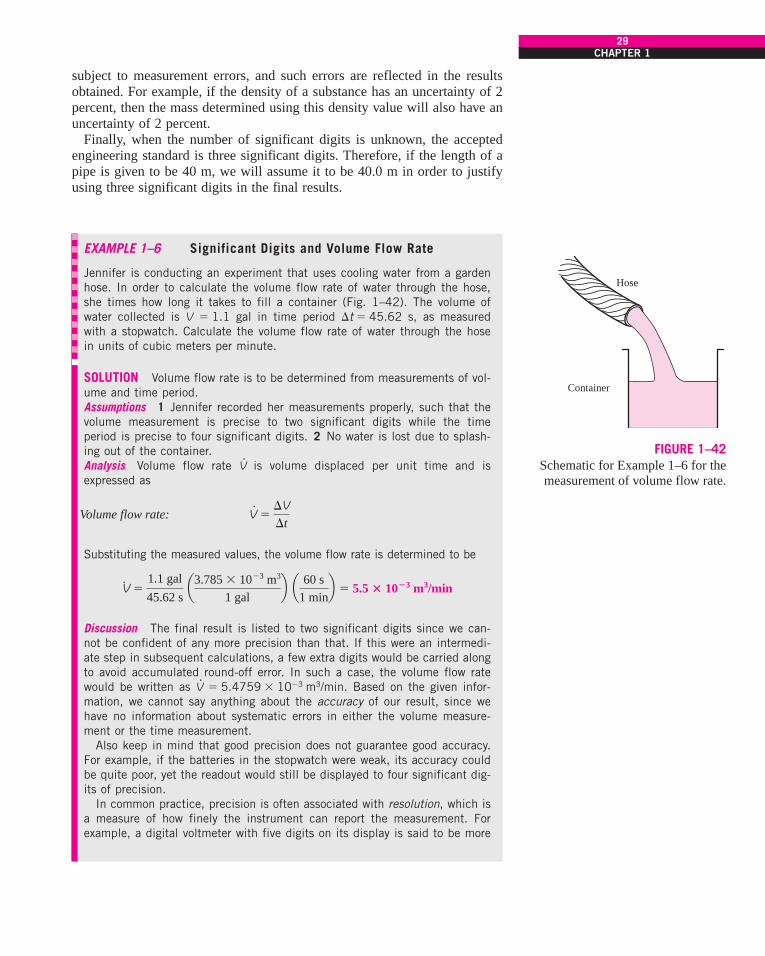
subject to measurement errors, and such errors are reflected in the resultsobtained. For example, if the density of a substance has an uncertainty of 2percent, then the mass determined using this density value will also have anuncertainty of 2 percent.

Finally, when the number of significant digits is unknown, the acceptedengineering standard is three significant digits. Therefore, if the length of apipe is given to be 40 m, we will assume it to be 40.0 m in order to justifyusing three significant digits in the final results.

EXAMPLE 1–6 Significant Digits and Volume Flow Rate

Jennifer is conducting an experiment that uses cooling water from a gardenhose. In order to calculate the volume flow rate of water through the hose,she times how long it takes to fill a container (Fig. 1–42). The volume ofwater collected is V ! 1.1 gal in time period )t ! 45.62 s, as measuredwith a stopwatch. Calculate the volume flow rate of water through the hosein units of cubic meters per minute.

SOLUTION Volume flow rate is to be determined from measurements of vol-ume and time period.Assumptions 1 Jennifer recorded her measurements properly, such that thevolume measurement is precise to two significant digits while the timeperiod is precise to four significant digits. 2 No water is lost due to splash-ing out of the container.Analysis Volume flow rate V

.is volume displaced per unit time and is

expressed as

Volume flow rate:

Substituting the measured values, the volume flow rate is determined to be

Discussion The final result is listed to two significant digits since we can-not be confident of any more precision than that. If this were an intermedi-ate step in subsequent calculations, a few extra digits would be carried alongto avoid accumulated round-off error. In such a case, the volume flow ratewould be written as V

.! 5.4759 ' 10$3 m3/min. Based on the given infor-

mation, we cannot say anything about the accuracy of our result, since wehave no information about systematic errors in either the volume measure-ment or the time measurement.

Also keep in mind that good precision does not guarantee good accuracy.For example, if the batteries in the stopwatch were weak, its accuracy couldbe quite poor, yet the readout would still be displayed to four significant dig-its of precision.

In common practice, precision is often associated with resolution, which isa measure of how finely the instrument can report the measurement. Forexample, a digital voltmeter with five digits on its display is said to be more

V#

!1.1 gal

45.62 s a3.785 ' 10$3 m3

1 galb a 60 s

1 minb ! 5.5 " 10#3 m3/min

V#!

)V)t

29CHAPTER 1

Container

Hose

FIGURE 1–42Schematic for Example 1–6 for themeasurement of volume flow rate.

cen72367_ch01.qxd 10/29/04 2:32 PM Page 29

precise than a digital voltmeter with only three digits. However, the numberof displayed digits has nothing to do with the overall accuracy of the mea-surement. An instrument can be very precise without being very accuratewhen there are significant bias errors. Likewise, an instrument with very fewdisplayed digits can be more accurate than one with many digits (Fig.1–43).

30FLUID MECHANICS

Exact time span = 45.623451 . . . s

(a)

TIMEXAM

46. s

(b)

TIMEXAM

43. s

(c)

TIMEXAM

44.189 s

(d)

TIMEXAM

45.624 s

FIGURE 1–43An instrument with many digits ofresolution (stopwatch c) may be lessaccurate than an instrument with fewdigits of resolution (stopwatch a).What can you say about stopwatches band d?

SUMMARY

In this chapter some basic concepts of fluid mechanics areintroduced and discussed. A substance in the liquid or gasphase is referred to as a fluid. Fluid mechanics is the sciencethat deals with the behavior of fluids at rest or in motion andthe interaction of fluids with solids or other fluids at theboundaries.

The flow of an unbounded fluid over a surface is externalflow, and the flow in a pipe or duct is internal flow if thefluid is completely bounded by solid surfaces. A fluid flow isclassified as being compressible or incompressible, depend-ing on the density variation of the fluid during flow. The den-sities of liquids are essentially constant, and thus the flow ofliquids is typically incompressible. The term steady impliesno change with time. The opposite of steady is unsteady, ortransient. The term uniform implies no change with locationover a specified region. A flow is said to be one-dimensionalwhen the velocity changes in one dimension only. A fluid indirect contact with a solid surface sticks to the surface and

there is no slip. This is known as the no-slip condition, whichleads to the formation of boundary layers along solid sur-faces.

A system of fixed mass is called a closed system, and asystem that involves mass transfer across its boundaries iscalled an open system or control volume. A large number ofengineering problems involve mass flow in and out of a sys-tem and are therefore modeled as control volumes.

In engineering calculations, it is important to pay particularattention to the units of the quantities to avoid errors causedby inconsistent units, and to follow a systematic approach. Itis also important to recognize that the information given isnot known to more than a certain number of significant dig-its, and the results obtained cannot possibly be accurate tomore significant digits. The information given on dimensionsand units; problem-solving technique; and accuracy, preci-sion, and significant digits will be used throughout the entiretext.

REFERENCES AND SUGGESTED READING

1. American Society for Testing and Materials. Standardsfor Metric Practice. ASTM E 380-79, January 1980.

2. C. T. Crowe, J. A. Roberson, and D. F. Elger. EngineeringFluid Mechanics, 7th ed. New York: Wiley, 2001.

3. R. W. Fox and A. T. McDonald. Introduction to FluidMechanics, 5th ed. New York: Wiley, 1999.

4. G. M. Homsy, H. Aref, K. S. Breuer, S. Hochgreb, J. R.Koseff, B. R. Munson, K. G. Powell, C. R. Robertson, andS. T. Thoroddsen. Multi-Media Fluid Mechanics (CD).Cambridge: Cambridge University Press, 2000.

5. M. Van Dyke. An Album of Fluid Motion. Stanford, CA:The Parabolic Press, 1982.

cen72367_ch01.qxd 10/29/04 2:32 PM Page 30

31CHAPTER 1

Guest Author: Lorenz Sigurdson, Vortex FluidDynamics Lab, University of Alberta

Why do the two images in Fig. 1–44 look alike? Figure 1–44b shows anabove-ground nuclear test performed by the U.S. Department of Energy in1957. An atomic blast created a fireball on the order of 100 m in diameter.Expansion is so quick that a compressible flow feature occurs: an expandingspherical shock wave. The image shown in Fig. 1–44a is an everydayinnocuous event: an inverted image of a dye-stained water drop after it hasfallen into a pool of water, looking from below the pool surface. It couldhave fallen from your spoon into a cup of coffee, or been a secondary splashafter a raindrop hit a lake. Why is there such a strong similarity betweenthese two vastly different events? The application of fundamental principlesof fluid mechanics learned in this book will help you understand much of theanswer, although one can go much deeper.

The water has higher density (Chap. 2) than air, so the drop has experi-enced negative buoyancy (Chap. 3) as it has fallen through the air beforeimpact. The fireball of hot gas is less dense than the cool air surrounding it,so it has positive buoyancy and rises. The shock wave (Chap. 12) reflectingfrom the ground also imparts a positive upward force to the fireball. The pri-mary structure at the top of each image is called a vortex ring. This ring is amini-tornado of concentrated vorticity (Chap. 4) with the ends of the tornadolooping around to close on itself. The laws of kinematics (Chap. 4) tell usthat this vortex ring will carry the fluid in a direction toward the top of thepage. This is expected in both cases from the forces applied and the law ofconservation of momentum applied through a control volume analysis (Chap.5). One could also analyze this problem with differential analysis (Chaps. 9and 10) or with computational fluid dynamics (Chap. 15). But why does theshape of the tracer material look so similar? This occurs if there is approxi-mate geometric and kinematic similarity (Chap. 7), and if the flow visualiza-tion (Chap. 4) technique is similar. The passive tracers of heat and dust forthe bomb, and fluorescent dye for the drop, were introduced in a similarmanner as noted in the figure caption.

Further knowledge of kinematics and vortex dynamics can help explain thesimilarity of the vortex structure in the images to much greater detail, as dis-cussed by Sigurdson (1997) and Peck and Sigurdson (1994). Look at thelobes dangling beneath the primary vortex ring, the striations in the “stalk,”and the ring at the base of each structure. There is also topological similarityof this structure to other vortex structures occurring in turbulence. Compari-son of the drop and bomb has given us a better understanding of how turbu-lent structures are created and evolve. What other secrets of fluid mechanicsare left to be revealed in explaining the similarity between these two flows?

ReferencesPeck, B., and Sigurdson, L.W., “The Three-Dimensional Vortex Structure of an Impacting Water

Drop,” Phys. Fluids, 6(2) (Part 1), p. 564, 1994.Peck, B., Sigurdson, L.W., Faulkner, B., and Buttar, I., “An Apparatus to Study Drop-Formed

Vortex Rings,” Meas. Sci. Tech., 6, p. 1538, 1995.Sigurdson, L.W., “Flow Visualization in Turbulent Large-Scale Structure Research,” Chapter 6

in Atlas of Visualization, Vol. III, Flow Visualization Society of Japan, eds., CRC Press,pp. 99–113, 1997.

FIGURE 1–44Comparison of the vortex structure

created by: (a) a water drop afterimpacting a pool of water (inverted,

from Peck and Sigurdson, 1994), and(b) an above-ground nuclear test in

Nevada in 1957 (U.S. Department ofEnergy). The 2.6 mm drop was dyed

with fluorescent tracer and illuminatedby a strobe flash 50 ms after it had

fallen 35 mm and impacted the clearpool. The drop was approximately

spherical at the time of impact withthe clear pool of water. Interruption of

a laser beam by the falling drop wasused to trigger a timer that controlled

the time of the strobe flash afterimpact of the drop. Details of the

careful experimental procedurenecessary to create the drop

photograph are given by Peck andSigurdson (1994) and Peck et al.

(1995). The tracers added to the flowin the bomb case were primarily heat

and dust. The heat is from the originalfireball which for this particular test

(the “Priscilla” event of OperationPlumbob) was large enough to reach

the ground from where the bomb wasinitially suspended. Therefore, thetracer’s initial geometric condition

was a sphere intersecting the ground.(a) From Peck, B., and Sigurdson, L. W.,

Phys. Fluids, 6(2)(Part 1), 564, 1994. Used by permission of the author.

(b) United States Department of Energy. Photo from Lorenz Sigurdson.

(a) (b)

APPLICATION SPOTLIGHT ! What Nuclear Blasts and Raindrops Have in Common

cen72367_ch01.qxd 10/29/04 2:32 PM Page 31

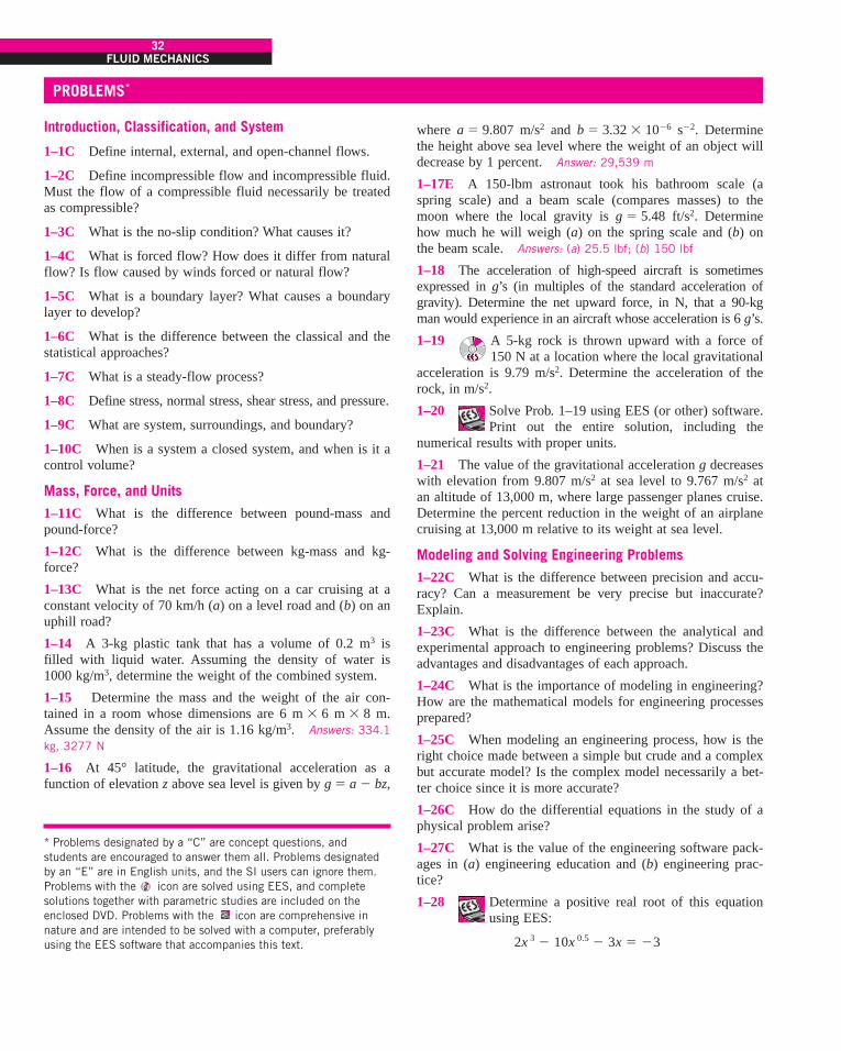
32FLUID MECHANICS

PROBLEMS*

Introduction, Classification, and System

1–1C Define internal, external, and open-channel flows.

1–2C Define incompressible flow and incompressible fluid.Must the flow of a compressible fluid necessarily be treatedas compressible?

1–3C What is the no-slip condition? What causes it?

1–4C What is forced flow? How does it differ from naturalflow? Is flow caused by winds forced or natural flow?

1–5C What is a boundary layer? What causes a boundarylayer to develop?

1–6C What is the difference between the classical and thestatistical approaches?

1–7C What is a steady-flow process?

1–8C Define stress, normal stress, shear stress, and pressure.

1–9C What are system, surroundings, and boundary?

1–10C When is a system a closed system, and when is it acontrol volume?

Mass, Force, and Units1–11C What is the difference between pound-mass andpound-force?

1–12C What is the difference between kg-mass and kg-force?

1–13C What is the net force acting on a car cruising at aconstant velocity of 70 km/h (a) on a level road and (b) on anuphill road?

1–14 A 3-kg plastic tank that has a volume of 0.2 m3 isfilled with liquid water. Assuming the density of water is1000 kg/m3, determine the weight of the combined system.

1–15 Determine the mass and the weight of the air con-tained in a room whose dimensions are 6 m ' 6 m ' 8 m.Assume the density of the air is 1.16 kg/m3. Answers: 334.1kg, 3277 N

1–16 At 45° latitude, the gravitational acceleration as afunction of elevation z above sea level is given by g ! a $ bz,

where a ! 9.807 m/s2 and b ! 3.32 ' 10$6 s$2. Determinethe height above sea level where the weight of an object willdecrease by 1 percent. Answer: 29,539 m

1–17E A 150-lbm astronaut took his bathroom scale (aspring scale) and a beam scale (compares masses) to themoon where the local gravity is g ! 5.48 ft/s2. Determinehow much he will weigh (a) on the spring scale and (b) onthe beam scale. Answers: (a) 25.5 lbf; (b) 150 lbf

1–18 The acceleration of high-speed aircraft is sometimesexpressed in g’s (in multiples of the standard acceleration ofgravity). Determine the net upward force, in N, that a 90-kgman would experience in an aircraft whose acceleration is 6 g’s.

1–19 A 5-kg rock is thrown upward with a force of150 N at a location where the local gravitational

acceleration is 9.79 m/s2. Determine the acceleration of therock, in m/s2.

1–20 Solve Prob. 1–19 using EES (or other) software.Print out the entire solution, including the

numerical results with proper units.

1–21 The value of the gravitational acceleration g decreaseswith elevation from 9.807 m/s2 at sea level to 9.767 m/s2 atan altitude of 13,000 m, where large passenger planes cruise.Determine the percent reduction in the weight of an airplanecruising at 13,000 m relative to its weight at sea level.

Modeling and Solving Engineering Problems1–22C What is the difference between precision and accu-racy? Can a measurement be very precise but inaccurate?Explain.

1–23C What is the difference between the analytical andexperimental approach to engineering problems? Discuss theadvantages and disadvantages of each approach.

1–24C What is the importance of modeling in engineering?How are the mathematical models for engineering processesprepared?

1–25C When modeling an engineering process, how is theright choice made between a simple but crude and a complexbut accurate model? Is the complex model necessarily a bet-ter choice since it is more accurate?

1–26C How do the differential equations in the study of aphysical problem arise?

1–27C What is the value of the engineering software pack-ages in (a) engineering education and (b) engineering prac-tice?

1–28 Determine a positive real root of this equationusing EES:

2x 3 $ 10x 0.5 $ 3x ! $3

* Problems designated by a “C” are concept questions, andstudents are encouraged to answer them all. Problems designatedby an “E” are in English units, and the SI users can ignore them.Problems with the icon are solved using EES, and completesolutions together with parametric studies are included on theenclosed DVD. Problems with the icon are comprehensive innature and are intended to be solved with a computer, preferablyusing the EES software that accompanies this text.

cen72367_ch01.qxd 10/29/04 2:32 PM Page 32

CHAPTER 133

1–29 Solve this system of two equations with twounknowns using EES:

1–30 Solve this system of three equations with threeunknowns using EES:

1–31 Solve this system of three equations with threeunknowns using EES:

Review Problems1–32 The weight of bodies may change somewhat from onelocation to another as a result of the variation of the gravita-

x & y $ z ! 2

x $ 3y 0.5 & xz ! $2

x 2y $ z ! 1

xy & 2z ! 8

3x 2 & 2y ! z & 2

2x $ y & z ! 5

3xy & y ! 3.5

x 3 $ y 2 ! 7.75

tional acceleration g with elevation. Accounting for this vari-ation using the relation in Prob. 1–16, determine the weightof an 80-kg person at sea level (z ! 0), in Denver (z ! 1610m), and on the top of Mount Everest (z ! 8848 m).

1–33 A man goes to a traditional market to buy a steak fordinner. He finds a 12-oz steak (1 lbm = 16 oz) for $3.15. Hethen goes to the adjacent international market and finds a320-g steak of identical quality for $2.80. Which steak is thebetter buy?

1–34 The reactive force developed by a jet engine to pushan airplane forward is called thrust, and the thrust developedby the engine of a Boeing 777 is about 85,000 lbf. Expressthis thrust in N and kgf.

Design and Essay Problem1–35 Write an essay on the various mass- and volume-mea-surement devices used throughout history. Also, explain thedevelopment of the modern units for mass and volume.

33CHAPTER 1

cen72367_ch01.qxd 10/29/04 2:32 PM Page 33

cen72367_ch01.qxd 10/29/04 2:32 PM Page 34

P R O P E R T I E S O F F L U I D S

In this chapter, we discuss properties that are encountered in the analysisof fluid flow. First we discuss intensive and extensive properties anddefine density and specific gravity. This is followed by a discussion of

the properties vapor pressure, energy and its various forms, the specificheats of ideal gases and incompressible substances, and the coefficient ofcompressibility. Then we discuss the property viscosity, which plays a dom-inant role in most aspects of fluid flow. Finally, we present the property sur-face tension and determine the capillary rise from static equilibrium condi-tions. The property pressure is discussed in Chap. 3 together with fluid statics.

35

CHAPTER

2OBJECTIVESWhen you finish reading this chapter, youshould be able to

! Have a working knowledge of thebasic properties of fluids andunderstand the continuumapproximation

! Have a working knowledge ofviscosity and the consequencesof the frictional effects it causesin fluid flow

! Calculate the capillary rises anddrops due to the surface tensioneffect

cen72367_ch02.qxd 10/29/04 2:20 PM Page 35

2–1 ! INTRODUCTIONAny characteristic of a system is called a property. Some familiar proper-ties are pressure P, temperature T, volume V, and mass m. The list can beextended to include less familiar ones such as viscosity, thermal conductiv-ity, modulus of elasticity, thermal expansion coefficient, electric resistivity,and even velocity and elevation.

Properties are considered to be either intensive or extensive. Intensiveproperties are those that are independent of the mass of a system, such astemperature, pressure, and density. Extensive properties are those whosevalues depend on the size—or extent—of the system. Total mass, total vol-ume V, and total momentum are some examples of extensive properties. Aneasy way to determine whether a property is intensive or extensive is todivide the system into two equal parts with an imaginary partition, as shownin Fig. 2–1. Each part will have the same value of intensive properties as theoriginal system, but half the value of the extensive properties.

Generally, uppercase letters are used to denote extensive properties (withmass m being a major exception), and lowercase letters are used for intensiveproperties (with pressure P and temperature T being the obvious exceptions).

Extensive properties per unit mass are called specific properties. Someexamples of specific properties are specific volume (v ! V/m) and specifictotal energy (e ! E/m).

The state of a system is described by its properties. But we know fromexperience that we do not need to specify all the properties in order to fix astate. Once the values of a sufficient number of properties are specified, therest of the properties assume certain values. That is, specifying a certainnumber of properties is sufficient to fix a state. The number of propertiesrequired to fix the state of a system is given by the state postulate: Thestate of a simple compressible system is completely specified by two inde-pendent, intensive properties.

Two properties are independent if one property can be varied while theother one is held constant. Not all properties are independent, and some aredefined in terms of others, as explained in Section 2–2.

ContinuumMatter is made up of atoms that are widely spaced in the gas phase. Yet it isvery convenient to disregard the atomic nature of a substance and view it asa continuous, homogeneous matter with no holes, that is, a continuum. Thecontinuum idealization allows us to treat properties as point functions and toassume that the properties vary continually in space with no jump disconti-nuities. This idealization is valid as long as the size of the system we dealwith is large relative to the space between the molecules. This is the case inpractically all problems, except some specialized ones. The continuum ide-alization is implicit in many statements we make, such as “the density ofwater in a glass is the same at any point.”

To have a sense of the distances involved at the molecular level, consider acontainer filled with oxygen at atmospheric conditions. The diameter of theoxygen molecule is about 3 " 10#10 m and its mass is 5.3 " 10#26 kg. Also,the mean free path of oxygen at 1 atm pressure and 20°C is 6.3 " 10#8 m.That is, an oxygen molecule travels, on average, a distance of 6.3 " 10#8 m(about 200 times its diameter) before it collides with another molecule.

36FLUID MECHANICS

!

mVTP

!

mVTP

12–12–

!

mV

TP

12–12–

Extensiveproperties

Intensiveproperties

FIGURE 2–1Criteria to differentiate intensive andextensive properties.

cen72367_ch02.qxd 10/29/04 2:20 PM Page 36

Also, there are about 2.5 " 1016 molecules of oxygen in the tiny volumeof 1 mm3 at 1 atm pressure and 20°C (Fig. 2–2). The continuum model isapplicable as long as the characteristic length of the system (such as itsdiameter) is much larger than the mean free path of the molecules. At veryhigh vacuums or very high elevations, the mean free path may become large(for example, it is about 0.1 m for atmospheric air at an elevation of 100km). For such cases the rarefied gas flow theory should be used, and theimpact of individual molecules should be considered. In this text we limitour consideration to substances that can be modeled as a continuum.

2–2 ! DENSITY AND SPECIFIC GRAVITYDensity is defined as mass per unit volume (Fig. 2–3). That is,

Density: (2–1)

The reciprocal of density is the specific volume v, which is defined as vol-ume per unit mass. That is, v ! V/m ! 1/r. For a differential volume ele-ment of mass dm and volume dV, density can be expressed as r ! dm/dV.

The density of a substance, in general, depends on temperature and pres-sure. The density of most gases is proportional to pressure and inverselyproportional to temperature. Liquids and solids, on the other hand, areessentially incompressible substances, and the variation of their density withpressure is usually negligible. At 20°C, for example, the density of waterchanges from 998 kg/m3 at 1 atm to 1003 kg/m3 at 100 atm, a change ofjust 0.5 percent. The density of liquids and solids depends more strongly ontemperature than it does on pressure. At 1 atm, for example, the density ofwater changes from 998 kg/m3 at 20°C to 975 kg/m3 at 75°C, a change of2.3 percent, which can still be neglected in many engineering analyses.

Sometimes the density of a substance is given relative to the density of awell-known substance. Then it is called specific gravity, or relative den-sity, and is defined as the ratio of the density of a substance to the density ofsome standard substance at a specified temperature (usually water at 4°C,for which rH2O ! 1000 kg/m3). That is,

Specific gravity: (2–2)

Note that the specific gravity of a substance is a dimensionless quantity.However, in SI units, the numerical value of the specific gravity of a sub-stance is exactly equal to its density in g/cm3 or kg/L (or 0.001 times thedensity in kg/m3) since the density of water at 4°C is 1 g/cm3 ! 1 kg/L !1000 kg/m3. The specific gravity of mercury at 0°C, for example, is 13.6.Therefore, its density at 0°C is 13.6 g/cm3 ! 13.6 kg/L ! 13,600 kg/m3.The specific gravities of some substances at 0°C are given in Table 2–1.Note that substances with specific gravities less than 1 are lighter thanwater, and thus they would float on water.

The weight of a unit volume of a substance is called specific weight andis expressed as

Specific weight: (2–3)

where g is the gravitational acceleration.

gs ! rg (N/m3)

SG !r

rH2O

r !mV (kg/m3)

37CHAPTER 2

VOID

1 atm, 20°CO2

3 " 1016 molecules/mm3

FIGURE 2–2Despite the large gaps between

molecules, a substance can be treatedas a continuum because of the very

large number of molecules even in anextremely small volume.

V = 12 m = 12 m3

! = 0.25 kg/m = 0.25 kg/m3

m = 3 kg = 3 kg

v = = = 4 m= 4 m3/kg/kg1–!

FIGURE 2–3Density is mass per unit volume;

specific volume is volume per unit mass.

TABLE 2–1Specific gravities of somesubstances at 0°C

Substance SG

Water 1.0Blood 1.05Seawater 1.025Gasoline 0.7Ethyl alcohol 0.79Mercury 13.6Wood 0.3–0.9Gold 19.2Bones 1.7–2.0Ice 0.92Air (at 1 atm) 0.0013

cen72367_ch02.qxd 10/29/04 2:20 PM Page 37

Recall from Chap. 1 that the densities of liquids are essentially constant,and thus they can often be approximated as being incompressible substancesduring most processes without sacrificing much in accuracy.

Density of Ideal GasesProperty tables provide very accurate and precise information about theproperties, but sometimes it is convenient to have some simple relationsamong the properties that are sufficiently general and accurate. Any equa-tion that relates the pressure, temperature, and density (or specific volume)of a substance is called an equation of state. The simplest and best-knownequation of state for substances in the gas phase is the ideal-gas equation ofstate, expressed as

(2–4)

where P is the absolute pressure, v is the specific volume, T is the thermody-namic (absolute) temperature, r is the density, and R is the gas constant. Thegas constant R is different for each gas and is determined from R ! Ru /M,where Ru is the universal gas constant whose value is Ru ! 8.314 kJ/kmol · K! 1.986 Btu/lbmol · R, and M is the molar mass (also called molecularweight) of the gas. The values of R and M for several substances are givenin Table A–1.

The thermodynamic temperature scale in the SI is the Kelvin scale, andthe temperature unit on this scale is the kelvin, designated by K. In the Eng-lish system, it is the Rankine scale, and the temperature unit on this scale isthe rankine, R. Various temperature scales are related to each other by

(2–5)

(2–6)

It is common practice to round the constants 273.15 and 459.67 to 273 and460, respectively.

Equation 2–4 is called the ideal-gas equation of state, or simply theideal-gas relation, and a gas that obeys this relation is called an ideal gas.For an ideal gas of volume V, mass m, and number of moles N ! m/M, theideal-gas equation of state can also be written as PV ! mRT or PV ! NRuT.For a fixed mass m, writing the ideal-gas relation twice and simplifying, theproperties of an ideal gas at two different states are related to each other byP1V1/T1 ! P2V2/T2.

An ideal gas is a hypothetical substance that obeys the relation Pv ! RT.It has been experimentally observed that the ideal-gas relation closelyapproximates the P-v-T behavior of real gases at low densities. At low pres-sures and high temperatures, the density of a gas decreases and the gasbehaves like an ideal gas. In the range of practical interest, many familiargases such as air, nitrogen, oxygen, hydrogen, helium, argon, neon, andkrypton and even heavier gases such as carbon dioxide can be treated asideal gases with negligible error (often less than 1 percent). Dense gasessuch as water vapor in steam power plants and refrigerant vapor in refriger-ators, however, should not be treated as ideal gases since they usually existat a state near saturation.

T(R) ! T($F) % 459.67

T(K) ! T($C) % 273.15

Pv ! RT or P ! rRT

38FLUID MECHANICS

cen72367_ch02.qxd 10/29/04 2:20 PM Page 38

EXAMPLE 2–1 Density, Specific Gravity, and Mass of Air in a Room

Determine the density, specific gravity, and mass of the air in a room whosedimensions are 4 m ! 5 m ! 6 m at 100 kPa and 25°C (Fig. 2–4).

Solution The density, specific gravity, and mass of the air in a room are tobe determined.Assumptions At specified conditions, air can be treated as an ideal gas.Properties The gas constant of air is R " 0.287 kPa ! m3/kg ! K.Analysis The density of air is determined from the ideal-gas relation P " rRTto be

Then the specific gravity of air becomes

Finally, the volume and the mass of air in the room are

Discussion Note that we converted the temperature to the unit K from °Cbefore using it in the ideal-gas relation.

2–3 ! VAPOR PRESSURE AND CAVITATIONIt is well-established that temperature and pressure are dependent propertiesfor pure substances during phase-change processes, and there is one-to-onecorrespondence between temperatures and pressures. At a given pressure, thetemperature at which a pure substance changes phase is called the satura-tion temperature Tsat. Likewise, at a given temperature, the pressure atwhich a pure substance changes phase is called the saturation pressure Psat.At an absolute pressure of 1 standard atmosphere (1 atm or 101.325 kPa),for example, the saturation temperature of water is 100°C. Conversely, at atemperature of 100°C, the saturation pressure of water is 1 atm.

The vapor pressure Pv of a pure substance is defined as the pressureexerted by its vapor in phase equilibrium with its liquid at a given tempera-ture. Pv is a property of the pure substance, and turns out to be identical tothe saturation pressure Psat of the liquid (Pv " Psat). We must be careful notto confuse vapor pressure with partial pressure. Partial pressure is definedas the pressure of a gas or vapor in a mixture with other gases. For example,atmospheric air is a mixture of dry air and water vapor, and atmosphericpressure is the sum of the partial pressure of dry air and the partial pressureof water vapor. The partial pressure of water vapor constitutes a small frac-tion (usually under 3 percent) of the atmospheric pressure since air is mostlynitrogen and oxygen. The partial pressure of a vapor must be less than orequal to the vapor pressure if there is no liquid present. However, when bothvapor and liquid are present and the system is in phase equilibrium, the par-tial pressure of the vapor must equal the vapor pressure, and the system issaid to be saturated. The rate of evaporation from open water bodies such as

m " rV " (1.17 kg/m3)(120 m3) " 140 kg

V " (4 m)(5 m)(6 m) " 120 m3

SG "r

rH2O"

1.17 kg/m3

1000 kg/m3 " 0.00117

r "P

RT"

100 kPa(0.287 kPa # m3/kg # K)(25 $ 273) K

" 1.17 kg/m3

39CHAPTER 2

6 m4 m

5 mAIRP =T =

100 kPa 25°C

FIGURE 2–4Schematic for Example 2–1.

cen72367_ch02.qxd 11/16/04 11:28 AM Page 39

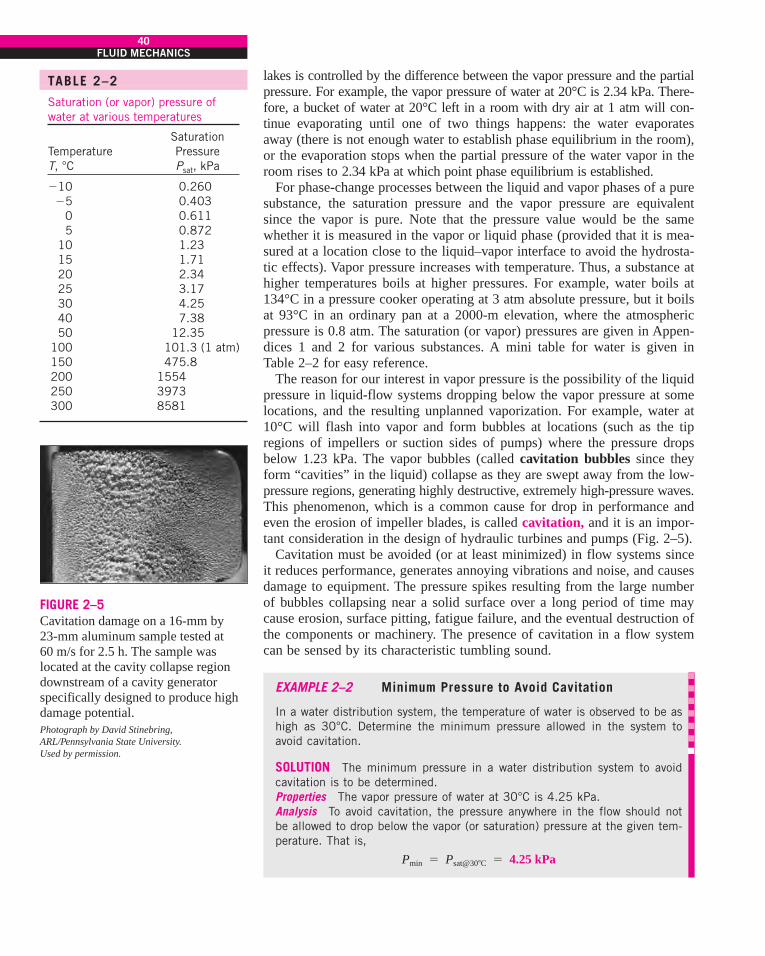
lakes is controlled by the difference between the vapor pressure and the partialpressure. For example, the vapor pressure of water at 20°C is 2.34 kPa. There-fore, a bucket of water at 20°C left in a room with dry air at 1 atm will con-tinue evaporating until one of two things happens: the water evaporatesaway (there is not enough water to establish phase equilibrium in the room),or the evaporation stops when the partial pressure of the water vapor in theroom rises to 2.34 kPa at which point phase equilibrium is established.

For phase-change processes between the liquid and vapor phases of a puresubstance, the saturation pressure and the vapor pressure are equivalentsince the vapor is pure. Note that the pressure value would be the samewhether it is measured in the vapor or liquid phase (provided that it is mea-sured at a location close to the liquid–vapor interface to avoid the hydrosta-tic effects). Vapor pressure increases with temperature. Thus, a substance athigher temperatures boils at higher pressures. For example, water boils at134°C in a pressure cooker operating at 3 atm absolute pressure, but it boilsat 93°C in an ordinary pan at a 2000-m elevation, where the atmosphericpressure is 0.8 atm. The saturation (or vapor) pressures are given in Appen-dices 1 and 2 for various substances. A mini table for water is given inTable 2–2 for easy reference.

The reason for our interest in vapor pressure is the possibility of the liquidpressure in liquid-flow systems dropping below the vapor pressure at somelocations, and the resulting unplanned vaporization. For example, water at10°C will flash into vapor and form bubbles at locations (such as the tipregions of impellers or suction sides of pumps) where the pressure dropsbelow 1.23 kPa. The vapor bubbles (called cavitation bubbles since theyform “cavities” in the liquid) collapse as they are swept away from the low-pressure regions, generating highly destructive, extremely high-pressure waves.This phenomenon, which is a common cause for drop in performance andeven the erosion of impeller blades, is called cavitation, and it is an impor-tant consideration in the design of hydraulic turbines and pumps (Fig. 2–5).

Cavitation must be avoided (or at least minimized) in flow systems sinceit reduces performance, generates annoying vibrations and noise, and causesdamage to equipment. The pressure spikes resulting from the large numberof bubbles collapsing near a solid surface over a long period of time maycause erosion, surface pitting, fatigue failure, and the eventual destruction ofthe components or machinery. The presence of cavitation in a flow systemcan be sensed by its characteristic tumbling sound.

EXAMPLE 2–2 Minimum Pressure to Avoid Cavitation

In a water distribution system, the temperature of water is observed to be ashigh as 30°C. Determine the minimum pressure allowed in the system toavoid cavitation.

SOLUTION The minimum pressure in a water distribution system to avoidcavitation is to be determined.Properties The vapor pressure of water at 30°C is 4.25 kPa.Analysis To avoid cavitation, the pressure anywhere in the flow should notbe allowed to drop below the vapor (or saturation) pressure at the given tem-perature. That is,

Pmin " Psat@30%C " 4.25 kPa

40FLUID MECHANICS

TABLE 2–2Saturation (or vapor) pressure ofwater at various temperatures

SaturationTemperature PressureT, °C Psat, kPa

&10 0.260&5 0.403

0 0.6115 0.872

10 1.2315 1.7120 2.3425 3.1730 4.2540 7.3850 12.35

100 101.3 (1 atm)150 475.8200 1554250 3973300 8581

FIGURE 2–5Cavitation damage on a 16-mm by 23-mm aluminum sample tested at 60 m/s for 2.5 h. The sample waslocated at the cavity collapse regiondownstream of a cavity generatorspecifically designed to produce highdamage potential.Photograph by David Stinebring,ARL/Pennsylvania State University.Used by permission.

cen72367_ch02.qxd 11/16/04 11:28 AM Page 40

Therefore, the pressure should be maintained above 4.25 kPa everywhere inthe flow.Discussion Note that the vapor pressure increases with increasing tempera-ture, and thus the risk of cavitation is greater at higher fluid temperatures.

2–4 ! ENERGY AND SPECIFIC HEATSEnergy can exist in numerous forms such as thermal, mechanical, kinetic,potential, electrical, magnetic, chemical, and nuclear, and their sum consti-tutes the total energy E (or e on a unit mass basis) of a system. The formsof energy related to the molecular structure of a system and the degree ofthe molecular activity are referred to as the microscopic energy. The sum ofall microscopic forms of energy is called the internal energy of a system,and is denoted by U (or u on a unit mass basis).

The macroscopic energy of a system is related to motion and the influ-ence of some external effects such as gravity, magnetism, electricity, andsurface tension. The energy that a system possesses as a result of its motionrelative to some reference frame is called kinetic energy. When all parts ofa system move with the same velocity, the kinetic energy per unit mass isexpressed as ke ! V 2/2 where V denotes the velocity of the system relativeto some fixed reference frame. The energy that a system possesses as aresult of its elevation in a gravitational field is called potential energy andis expressed on a per-unit mass basis as pe ! gz where g is the gravitationalacceleration and z is the elevation of the center of gravity of a system rela-tive to some arbitrarily selected reference plane.

In daily life, we frequently refer to the sensible and latent forms of inter-nal energy as heat, and we talk about the heat content of bodies. In engi-neering, however, those forms of energy are usually referred to as thermalenergy to prevent any confusion with heat transfer.

The international unit of energy is the joule (J) or kilojoule (1 kJ ! 1000 J).In the English system, the unit of energy is the British thermal unit (Btu),which is defined as the energy needed to raise the temperature of 1 lbm ofwater at 68°F by 1°F. The magnitudes of kJ and Btu are almost identical(1 Btu ! 1.0551 kJ). Another well-known unit of energy is the calorie(1 cal ! 4.1868 J), which is defined as the energy needed to raise the tem-perature of 1 g of water at 14.5°C by 1°C.

In the analysis of systems that involve fluid flow, we frequently encounterthe combination of properties u and Pv. For convenience, this combinationis called enthalpy h. That is,

Enthalpy: (2–7)

where P/r is the flow energy, also called the flow work, which is the energyper unit mass needed to move the fluid and maintain flow. In the energyanalysis of flowing fluids, it is convenient to treat the flow energy as part ofthe energy of the fluid and to represent the microscopic energy of a fluidstream by enthalpy h (Fig. 2–6). Note that enthalpy is a quantity per unitmass, and thus it is a specific property.

In the absence of such effects as magnetic, electric, and surface tension, asystem is called a simple compressible system. The total energy of a simple

h ! u % Pv ! u %Pr

41CHAPTER 2

Energy = hFlowing fluid

Energy = uStationary fluid

FIGURE 2–6The internal energy u represents themicroscopic energy of a nonflowing

fluid per unit mass, whereas enthalpyh represents the microscopic energy of

a flowing fluid per unit mass.

cen72367_ch02.qxd 10/29/04 2:20 PM Page 41

compressible system consists of three parts: internal, kinetic, and potentialenergies. On a unit-mass basis, it is expressed as e ! u % ke % pe. Thefluid entering or leaving a control volume possesses an additional form ofenergy—the flow energy P/r. Then the total energy of a flowing fluid on aunit-mass basis becomes

(2–8)

where h ! P/r % u is the enthalpy, V is the velocity, and z is the elevationof the system relative to some external reference point.

By using the enthalpy instead of the internal energy to represent the energyof a flowing fluid, one does not need to be concerned about the flow work.The energy associated with pushing the fluid is automatically taken care of byenthalpy. In fact, this is the main reason for defining the property enthalpy.

The differential and finite changes in the internal energy and enthalpy ofan ideal gas can be expressed in terms of the specific heats as

(2–9)

where cv and cp are the constant-volume and constant-pressure specific heats ofthe ideal gas. Using specific heat values at the average temperature, the finitechanges in internal energy and enthalpy can be expressed approximately as

(2–10)

For incompressible substances, the constant-volume and constant-pressurespecific heats are identical. Therefore, cp ! cv ! c for liquids, and thechange in the internal energy of liquids can be expressed as &u ! cave &T.

Noting that r ! constant for incompressible substances, the differentia-tion of enthalpy h ! u % P/r gives dh ! du % dP/r. Integrating, theenthalpy change becomes

(2–11)

Therefore, &h ! &u ! cave &T for constant-pressure processes, and &h !&P/r for constant-temperature processes of liquids.

2–5 ! COEFFICIENT OF COMPRESSIBILITYWe know from experience that the volume (or density) of a fluid changeswith a change in its temperature or pressure. Fluids usually expand as theyare heated or depressurized and contract as they are cooled or pressurized.But the amount of volume change is different for different fluids, and weneed to define properties that relate volume changes to the changes in pres-sure and temperature. Two such properties are the bulk modulus of elasticityk and the coefficient of volume expansion b.

It is a common observation that a fluid contracts when more pressure isapplied on it and expands when the pressure acting on it is reduced (Fig.2–7). That is, fluids act like elastic solids with respect to pressure. Therefore,in an analogous manner to Young’s modulus of elasticity for solids, it isappropriate to define a coefficient of compressibility k (also called the bulkmodulus of compressibility or bulk modulus of elasticity) for fluids as

(2–12)k ! #v a'P'vb

T ! ra'P

'rb

T (Pa)

&h ! &u % &P/r ! cave &T % &P/r

&u ! cv,ave &T and &h ! cp,ave &T

du ! cv dT and dh ! cp dT

eflowing ! P/r % e ! h % ke % pe ! h %V 2

2% gz (kJ/kg)

42FLUID MECHANICS

P2 > P1

P1

FIGURE 2–7Fluids, like solids, compress when the applied pressure is increased from P1 to P2.

cen72367_ch02.qxd 10/29/04 2:20 PM Page 42

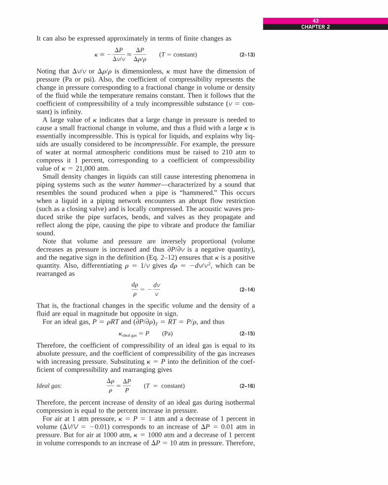
It can also be expressed approximately in terms of finite changes as

(2–13)

Noting that &v/v or &r/r is dimensionless, k must have the dimension ofpressure (Pa or psi). Also, the coefficient of compressibility represents thechange in pressure corresponding to a fractional change in volume or densityof the fluid while the temperature remains constant. Then it follows that thecoefficient of compressibility of a truly incompressible substance (v ! con-stant) is infinity.

A large value of k indicates that a large change in pressure is needed tocause a small fractional change in volume, and thus a fluid with a large k isessentially incompressible. This is typical for liquids, and explains why liq-uids are usually considered to be incompressible. For example, the pressureof water at normal atmospheric conditions must be raised to 210 atm tocompress it 1 percent, corresponding to a coefficient of compressibilityvalue of k ! 21,000 atm.

Small density changes in liquids can still cause interesting phenomena inpiping systems such as the water hammer—characterized by a sound thatresembles the sound produced when a pipe is “hammered.” This occurswhen a liquid in a piping network encounters an abrupt flow restriction(such as a closing valve) and is locally compressed. The acoustic waves pro-duced strike the pipe surfaces, bends, and valves as they propagate andreflect along the pipe, causing the pipe to vibrate and produce the familiarsound.

Note that volume and pressure are inversely proportional (volumedecreases as pressure is increased and thus #P/#v is a negative quantity),and the negative sign in the definition (Eq. 2–12) ensures that k is a positivequantity. Also, differentiating r ! 1/v gives dr ! #dv/v2, which can berearranged as

(2–14)

That is, the fractional changes in the specific volume and the density of afluid are equal in magnitude but opposite in sign.

For an ideal gas, P ! rRT and (#P/#r)T ! RT ! P/r, and thus

(2–15)

Therefore, the coefficient of compressibility of an ideal gas is equal to itsabsolute pressure, and the coefficient of compressibility of the gas increaseswith increasing pressure. Substituting k ! P into the definition of the coef-ficient of compressibility and rearranging gives

Ideal gas: (2–16)

Therefore, the percent increase of density of an ideal gas during isothermalcompression is equal to the percent increase in pressure.

For air at 1 atm pressure, k ! P ! 1 atm and a decrease of 1 percent involume (&V/V ! #0.01) corresponds to an increase of &P ! 0.01 atm inpressure. But for air at 1000 atm, k ! 1000 atm and a decrease of 1 percentin volume corresponds to an increase of &P ! 10 atm in pressure. Therefore,

&r

r!

&PP

(T ! constant)

kideal gas ! P (Pa)

drr

! #dvv

k ! #&P

&v/v!

&P&r/r

(T ! constant)

43CHAPTER 2

cen72367_ch02.qxd 10/29/04 2:20 PM Page 43

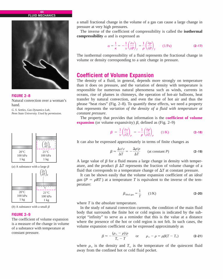
a small fractional change in the volume of a gas can cause a large change inpressure at very high pressures.

The inverse of the coefficient of compressibility is called the isothermalcompressibility a and is expressed as

(2–17)

The isothermal compressibility of a fluid represents the fractional change involume or density corresponding to a unit change in pressure.

Coefficient of Volume ExpansionThe density of a fluid, in general, depends more strongly on temperaturethan it does on pressure, and the variation of density with temperature isresponsible for numerous natural phenomena such as winds, currents inoceans, rise of plumes in chimneys, the operation of hot-air balloons, heattransfer by natural convection, and even the rise of hot air and thus thephrase “heat rises” (Fig. 2–8). To quantify these effects, we need a propertythat represents the variation of the density of a fluid with temperature atconstant pressure.

The property that provides that information is the coefficient of volumeexpansion (or volume expansivity) b, defined as (Fig. 2–9)

(2–18)

It can also be expressed approximately in terms of finite changes as

(2–19)

A large value of b for a fluid means a large change in density with temper-ature, and the product b &T represents the fraction of volume change of afluid that corresponds to a temperature change of &T at constant pressure.

It can be shown easily that the volume expansion coefficient of an idealgas (P ! rRT ) at a temperature T is equivalent to the inverse of the tem-perature:

(2–20)

where T is the absolute temperature.In the study of natural convection currents, the condition of the main fluid

body that surrounds the finite hot or cold regions is indicated by the sub-script “infinity” to serve as a reminder that this is the value at a distancewhere the presence of the hot or cold region is not felt. In such cases, thevolume expansion coefficient can be expressed approximately as

(2–21)

where r( is the density and T( is the temperature of the quiescent fluidaway from the confined hot or cold fluid pocket.

b " #(r( # r)/r

T( # T or r( # r ! rb(T # T()

bideal gas !1T

(1/K)

b "&v/v&T

! #&r/r&T

(at constant P)

b ! 1v a'v

'Tb

P ! #

1r

a'r'Tb

P (1/K)

a !1k

! #1v a'v

'Pb

T!

1r

a'r'Pb

T (1/Pa)

44FLUID MECHANICS

FIGURE 2–8Natural convection over a woman’shand. G. S. Settles, Gas Dynamics Lab,Penn State University. Used by permission.

20°C100 kPa

1 kg

21°C100 kPa

1 kg

20°C100 kPa

1 kg

21°C100 kPa

1 kg

# –––#TQ R

Q RP

# –––#T P

(a) A substance with a large b

(b) A substance with a small b

v

v

FIGURE 2–9The coefficient of volume expansion is a measure of the change in volumeof a substance with temperature atconstant pressure.

cen72367_ch02.qxd 10/29/04 2:20 PM Page 44

We will see in Chap. 3 that natural convection currents are initiated by thebuoyancy force, which is proportional to the density difference, which isproportional to the temperature difference at constant pressure. Therefore,the larger the temperature difference between the hot or cold fluid pocketand the surrounding main fluid body, the larger the buoyancy force and thusthe stronger the natural convection currents.

The combined effects of pressure and temperature changes on the volumechange of a fluid can be determined by taking the specific volume to be afunction of T and P. Differentiating v ! v(T, P) and using the definitions ofthe compression and expansion coefficients a and b give

(2–22)

Then the fractional change in volume (or density) due to changes in pres-sure and temperature can be expressed approximately as

(2–23)

EXAMPLE 2–3 Variation of Density with Temperature and Pressure

Consider water initially at 20°C and 1 atm. Determine the final density ofwater (a) if it is heated to 50°C at a constant pressure of 1 atm, and (b) if itis compressed to 100-atm pressure at a constant temperature of 20°C. Takethe isothermal compressibility of water to be a ! 4.80 " 10#5 atm#1.

SOLUTION Water at a given temperature and pressure is considered. Thedensities of water after it is heated and after it is compressed are to bedetermined.Assumptions 1 The coefficient of volume expansion and the isothermalcompressibility of water are constant in the given temperature range. 2 Anapproximate analysis is performed by replacing differential changes in quan-tities by finite changes.Properties The density of water at 20°C and 1 atm pressure is r1 !998.0 kg/m3. The coefficient of volume expansion at the average tempera-ture of (20 % 50)/2 ! 35°C is b ! 0.337 " 10#3 K#1. The isothermal com-pressibility of water is given to be a ! 4.80 " 10#5 atm#1.Analysis When differential quantities are replaced by differences and theproperties a and b are assumed to be constant, the change in density interms of the changes in pressure and temperature is expressed approxi-mately as (Eq. 2–23)

(a) The change in density due to the change of temperature from 20°C to50°C at constant pressure is

Noting that &r ! r2 # r1, the density of water at 50°C and 1 atm is

r2 ! r1 % &r ! 998.0 % (#10.0) ! 988.0 kg/m3

! #10.0 kg/m3

&r ! #br &T ! #(0.337 " 10#3 K#1)(998 kg/m3)(50 # 20) K

&r ! ar &P # br &T

&vv

! #&r

r ! b &T # a &P

dv ! a'v'Tb

P dT % a'v

'Pb

T dP ! (b dT # a dP)v

45CHAPTER 2

cen72367_ch02.qxd 10/29/04 2:20 PM Page 45

which is almost identical to the listed value of 988.1 kg/m3 at 50°C in TableA–3. This is mostly due to b varying with temperature almost linearly, asshown in Fig. 2–10.

(b) The change in density due to a change of pressure from 1 atm to 100atm at constant temperature is

Then the density of water at 100 atm and 20°C becomes

Discussion Note that the density of water decreases while being heated andincreases while being compressed, as expected. This problem can be solvedmore accurately using differential analysis when functional forms of proper-ties are available.

2–6 ! VISCOSITYWhen two solid bodies in contact move relative to each other, a frictionforce develops at the contact surface in the direction opposite to motion. Tomove a table on the floor, for example, we have to apply a force to the tablein the horizontal direction large enough to overcome the friction force. Themagnitude of the force needed to move the table depends on the frictioncoefficient between the table and the floor.

The situation is similar when a fluid moves relative to a solid or when twofluids move relative to each other. We move with relative ease in air, but notso in water. Moving in oil would be even more difficult, as can be observedby the slower downward motion of a glass ball dropped in a tube filled withoil. It appears that there is a property that represents the internal resistanceof a fluid to motion or the “fluidity,” and that property is the viscosity. Theforce a flowing fluid exerts on a body in the flow direction is called thedrag force, and the magnitude of this force depends, in part, on viscosity(Fig. 2–11).

To obtain a relation for viscosity, consider a fluid layer between two verylarge parallel plates (or equivalently, two parallel plates immersed in a largebody of a fluid) separated by a distance ! (Fig. 2–12). Now a constant par-allel force F is applied to the upper plate while the lower plate is held fixed.After the initial transients, it is observed that the upper plate moves continu-ously under the influence of this force at a constant velocity V. The fluid incontact with the upper plate sticks to the plate surface and moves with it atthe same velocity, and the shear stress t acting on this fluid layer is

(2–24)

where A is the contact area between the plate and the fluid. Note that thefluid layer deforms continuously under the influence of shear stress.

The fluid in contact with the lower plate assumes the velocity of that plate,which is zero (again because of the no-slip condition). In steady laminar

t !FA

r2 ! r1 % &r ! 998.0 % 4.7 ! 1002.7 kg/m3

&r ! ar &P ! (4.80 " 10#5 atm#1)(998 kg/m3)(100 # 1) atm ! 4.7 kg/m3

46FLUID MECHANICS

0.00050

0.00020

T, °C50454035302520

0.00025

0.00030

0.00035

0.00040

0.00045

b, 1

/K

FIGURE 2–10The variation of the coefficient ofvolume expansion of water b withtemperature in the range of 20°C to 50°C. Data were generated and plotted using EES.

Air

Water

Dragforce

Dragforce

V

V

FIGURE 2–11A fluid moving relative to a bodyexerts a drag force on the body, partlybecause of friction caused by viscosity.

cen72367_ch02.qxd 10/29/04 2:20 PM Page 46

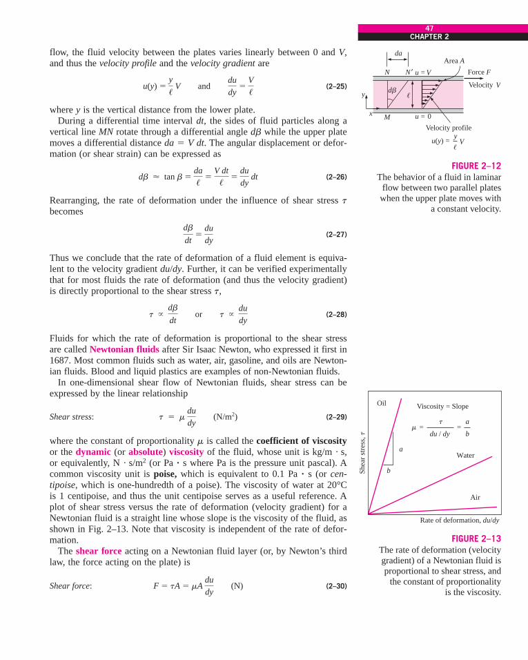
flow, the fluid velocity between the plates varies linearly between 0 and V,and thus the velocity profile and the velocity gradient are

(2–25)

where y is the vertical distance from the lower plate.During a differential time interval dt, the sides of fluid particles along a

vertical line MN rotate through a differential angle db while the upper platemoves a differential distance da ! V dt. The angular displacement or defor-mation (or shear strain) can be expressed as

(2–26)

Rearranging, the rate of deformation under the influence of shear stress tbecomes

(2–27)

Thus we conclude that the rate of deformation of a fluid element is equiva-lent to the velocity gradient du/dy. Further, it can be verified experimentallythat for most fluids the rate of deformation (and thus the velocity gradient)is directly proportional to the shear stress t,

(2–28)

Fluids for which the rate of deformation is proportional to the shear stressare called Newtonian fluids after Sir Isaac Newton, who expressed it first in1687. Most common fluids such as water, air, gasoline, and oils are Newton-ian fluids. Blood and liquid plastics are examples of non-Newtonian fluids.

In one-dimensional shear flow of Newtonian fluids, shear stress can beexpressed by the linear relationship

Shear stress: (2–29)

where the constant of proportionality m is called the coefficient of viscosityor the dynamic (or absolute) viscosity of the fluid, whose unit is kg/m · s,or equivalently, N · s/m2 (or Pa ! s where Pa is the pressure unit pascal). Acommon viscosity unit is poise, which is equivalent to 0.1 Pa ! s (or cen-tipoise, which is one-hundredth of a poise). The viscosity of water at 20°Cis 1 centipoise, and thus the unit centipoise serves as a useful reference. Aplot of shear stress versus the rate of deformation (velocity gradient) for aNewtonian fluid is a straight line whose slope is the viscosity of the fluid, asshown in Fig. 2–13. Note that viscosity is independent of the rate of defor-mation.

The shear force acting on a Newtonian fluid layer (or, by Newton’s thirdlaw, the force acting on the plate) is

Shear force: (2–30)F ! tA ! mA dudy

(N)

t ! m dudy

(N/m2)

t ) db

dt or t )

dudy

db

dt!

dudy

db " tan b !da/ !

V dt/ !

dudy

dt

u(y) !y

/ V and dudy

!V/

47CHAPTER 2

V

V

V

u(y) =

u = 0

u =

y

!

!

N

da

M

N $

Velocity profile

Force F

x

y dbVelocity

Area A

FIGURE 2–12The behavior of a fluid in laminar

flow between two parallel plates when the upper plate moves with

a constant velocity.

Rate of deformation, du/dy

Shea

r str

ess,

t

Oil

Water

Air

Viscosity = Slope

= =

a

a

b

bdu / dy

tm

FIGURE 2–13The rate of deformation (velocitygradient) of a Newtonian fluid isproportional to shear stress, and

the constant of proportionality is the viscosity.

cen72367_ch02.qxd 10/29/04 2:20 PM Page 47

where again A is the contact area between the plate and the fluid. Then theforce F required to move the upper plate in Fig. 2–12 at a constant velocityof V while the lower plate remains stationary is

(2–31)

This relation can alternately be used to calculate m when the force F is mea-sured. Therefore, the experimental setup just described can be used to mea-sure the viscosity of fluids. Note that under identical conditions, the force Fwill be very different for different fluids.

For non-Newtonian fluids, the relationship between shear stress and rateof deformation is not linear, as shown in Fig. 2–14. The slope of the curveon the t versus du/dy chart is referred to as the apparent viscosity of thefluid. Fluids for which the apparent viscosity increases with the rate ofdeformation (such as solutions with suspended starch or sand) are referredto as dilatant or shear thickening fluids, and those that exhibit the oppositebehavior (the fluid becoming less viscous as it is sheared harder, such assome paints, polymer solutions, and fluids with suspended particles) arereferred to as pseudoplastic or shear thinning fluids. Some materials such astoothpaste can resist a finite shear stress and thus behave as a solid, butdeform continuously when the shear stress exceeds the yield stress and thusbehave as a fluid. Such materials are referred to as Bingham plastics afterE. C. Bingham, who did pioneering work on fluid viscosity for the U.S.National Bureau of Standards in the early twentieth century.

In fluid mechanics and heat transfer, the ratio of dynamic viscosity todensity appears frequently. For convenience, this ratio is given the namekinematic viscosity n and is expressed as n ! m/r. Two common units ofkinematic viscosity are m2/s and stoke (1 stoke ! 1 cm2/s ! 0.0001 m2/s).

In general, the viscosity of a fluid depends on both temperature and pres-sure, although the dependence on pressure is rather weak. For liquids, boththe dynamic and kinematic viscosities are practically independent of pres-sure, and any small variation with pressure is usually disregarded, except atextremely high pressures. For gases, this is also the case for dynamic vis-cosity (at low to moderate pressures), but not for kinematic viscosity sincethe density of a gas is proportional to its pressure (Fig. 2–15).

The viscosity of a fluid is a measure of its “resistance to deformation.”Viscosity is due to the internal frictional force that develops between differ-ent layers of fluids as they are forced to move relative to each other. Viscos-ity is caused by the cohesive forces between the molecules in liquids and bythe molecular collisions in gases, and it varies greatly with temperature. Theviscosity of liquids decreases with temperature, whereas the viscosity ofgases increases with temperature (Fig. 2–16). This is because in a liquid themolecules possess more energy at higher temperatures, and they can opposethe large cohesive intermolecular forces more strongly. As a result, the ener-gized liquid molecules can move more freely.

In a gas, on the other hand, the intermolecular forces are negligible, andthe gas molecules at high temperatures move randomly at higher velocities.This results in more molecular collisions per unit volume per unit time andtherefore in greater resistance to flow. The viscosity of a fluid is directly

F ! mA V/ (N)

48FLUID MECHANICS

Rate of deformation, du/dy

Shea

r str

ess,

t

Binghamplastic

Pseudoplastic

Newtonian

Dilatant

FIGURE 2–14Variation of shear stress with the rateof deformation for Newtonian andnon-Newtonian fluids (the slope of acurve at a point is the apparentviscosity of the fluid at that point).

Air at 20°C and 1 atm:m= 1.83 " 10–5 kg/m % s = 1.52 " 10–5 m2/s

Air at 20°C and 4 atm:m= 1.83 " 10–5 kg/m % s = 0.380 " 10–5 m2/s

*

*

FIGURE 2–15Dynamic viscosity, in general, doesnot depend on pressure, but kinematicviscosity does.

cen72367_ch02.qxd 10/29/04 2:20 PM Page 48

related to the pumping power needed to transport a fluid in a pipe or tomove a body (such as a car in air or a submarine in the sea) through a fluid.

The kinetic theory of gases predicts the viscosity of gases to be propor-tional to the square root of temperature. That is, . This predictionis confirmed by practical observations, but deviations for different gasesneed to be accounted for by incorporating some correction factors. The vis-cosity of gases is expressed as a function of temperature by the Sutherlandcorrelation (from The U.S. Standard Atmosphere) as

Gases: (2–32)

where T is absolute temperature and a and b are experimentally determinedconstants. Note that measuring viscosities at two different temperatures issufficient to determine these constants. For air, the values of these constantsare a ! 1.458 " 10#6 kg/(m ! s ! K1/2) and b ! 110.4 K at atmosphericconditions. The viscosity of gases is independent of pressure at low to mod-erate pressures (from a few percent of 1 atm to several atm). But viscosityincreases at high pressures due to the increase in density.

For liquids, the viscosity is approximated as

Liquids: (2–33)

where again T is absolute temperature and a, b, and c are experimentallydetermined constants. For water, using the values a ! 2.414 " 10#5 N ! s/m2,b ! 247.8 K, and c ! 140 K results in less than 2.5 percent error in viscosityin the temperature range of 0°C to 370°C (Touloukian et al., 1975).

Consider a fluid layer of thickness ! within a small gap between two con-centric cylinders, such as the thin layer of oil in a journal bearing. The gapbetween the cylinders can be modeled as two parallel flat plates separated bya fluid. Noting that torque is T ! FR (force times the moment arm, which isthe radius R of the inner cylinder in this case), the tangential velocity is V !vR (angular velocity times the radius), and taking the wetted surface area ofthe inner cylinder to be A ! 2pRL by disregarding the shear stress acting onthe two ends of the inner cylinder, torque can be expressed as

(2–34)

where L is the length of the cylinder and n. is the number of revolutions perunit time, which is usually expressed in rpm (revolutions per minute). Notethat the angular distance traveled during one rotation is 2p rad, and thus therelation between the angular velocity in rad/min and the rpm is v ! 2pn..Equation 2–34 can be used to calculate the viscosity of a fluid by measuringtorque at a specified angular velocity. Therefore, two concentric cylinderscan be used as a viscometer, a device that measures viscosity.

The viscosities of some fluids at room temperature are listed in Table 2–3.They are plotted against temperature in Fig. 2–17. Note that the viscositiesof different fluids differ by several orders of magnitude. Also note that it ismore difficult to move an object in a higher-viscosity fluid such as engine oilthan it is in a lower-viscosity fluid such as water. Liquids, in general, aremuch more viscous than gases.

T ! FR ! m 2pR3vL/ ! m

4p 2R3n#L

/

m ! a10b/(T#c)

m !aT1/2

1 % b/T

mgas ) 1T

49CHAPTER 2

Liquids

Gases

Temperature

Viscosity

FIGURE 2–16The viscosity of liquids decreases

and the viscosity of gases increaseswith temperature.

TABLE 2–3Dynamic viscosities of some fluidsat 1 atm and 20°C (unlessotherwise stated)

Dynamic Viscosity Fluid m, kg/m ! s

Glycerin:#20°C 134.0

0°C 10.520°C 1.5240°C 0.31

Engine oil:SAE 10W 0.10SAE 10W30 0.17SAE 30 0.29SAE 50 0.86

Mercury 0.0015Ethyl alcohol 0.0012Water:

0°C 0.001820°C 0.0010

100°C (liquid) 0.00028100°C (vapor) 0.000012

Blood, 37$C 0.00040Gasoline 0.00029Ammonia 0.00015Air 0.000018Hydrogen, 0°C 0.0000088

cen72367_ch02.qxd 10/29/04 2:20 PM Page 49

EXAMPLE 2–4 Determining the Viscosity of a Fluid

The viscosity of a fluid is to be measured by a viscometer constructed of two40-cm-long concentric cylinders (Fig. 2–18). The outer diameter of the innercylinder is 12 cm, and the gap between the two cylinders is 0.15 cm. Theinner cylinder is rotated at 300 rpm, and the torque is measured to be1.8 N ! m. Determine the viscosity of the fluid.

SOLUTION The torque and the rpm of a double cylinder viscometer aregiven. The viscosity of the fluid is to be determined.Assumptions 1 The inner cylinder is completely submerged in oil. 2 Theviscous effects on the two ends of the inner cylinder are negligible.Analysis The velocity profile is linear only when the curvature effects arenegligible, and the profile can be approximated as being linear in this casesince !/R ++ 1. Solving Eq. 2–34 for viscosity and substituting the givenvalues, the viscosity of the fluid is determined to be

m !T/

4p 2R3n#L

!(1.8 N , m)(0.0015 m)

4p 2(0.06 m)3(300/60 1/s)(0.4 m)! 0.158 N , s /m2

50FLUID MECHANICS

0.50.40.30.2

SAE 10 oil

Crude oil (SG 0.86)

KeroseneAniline

Mercury

Castor oil

SAE 30 oil

Glycerin

0.1

0.060.040.030.02

0.01

Abs

olut

e vi

scos

ity m

, N %

s/m

2

6432

1 " 10–3

6432

1 " 10–4

432

1 " 10–5

5–20 0 20 40

Temperature, °C60 80 100 120

6

Carbon tetrachloride

Ethyl alcoholWater

Gasoline (SG 0.68)

Helium

Air Carbon Dioxide

Hydrogen

Benzene

FIGURE 2–17The variation of dynamic (absolute)viscosities of common fluids withtemperature at 1 atm (1 N ! s/m2 ! 1 kg/m ! s ! 0.020886 lbf ! s/ft2).F. M. White, Fluid Mechanics 4e. Copyright © 1999 The McGraw-Hill Companies,Inc. Used by permission.

R

Shaft

Stationarycylinder

Fluid

!

n = 300 rpm%

FIGURE 2–18Schematic for Example 2–4.

cen72367_ch02.qxd 10/29/04 2:20 PM Page 50

Discussion Viscosity is a strong function of temperature, and a viscosityvalue without a corresponding temperature is of little value. Therefore, thetemperature of the fluid should have also been measured during this experi-ment, and reported with this calculation.

2–7 ! SURFACE TENSION AND CAPILLARY EFFECTIt is often observed that a drop of blood forms a hump on a horizontal glass;a drop of mercury forms a near-perfect sphere and can be rolled just like asteel ball over a smooth surface; water droplets from rain or dew hang frombranches or leaves of trees; a liquid fuel injected into an engine forms amist of spherical droplets; water dripping from a leaky faucet falls as spher-ical droplets; a soap bubble released into the air forms a spherical shape;and water beads up into small drops on flower petals (Fig. 2–19).

In these and other observances, liquid droplets behave like small sphericalballoons filled with the liquid, and the surface of the liquid acts like astretched elastic membrane under tension. The pulling force that causes thistension acts parallel to the surface and is due to the attractive forcesbetween the molecules of the liquid. The magnitude of this force per unitlength is called surface tension ss and is usually expressed in the unit N/m(or lbf/ft in English units). This effect is also called surface energy and isexpressed in the equivalent unit of N ! m/m2 or J/m2. In this case, ss repre-sents the stretching work that needs to be done to increase the surface areaof the liquid by a unit amount.

To visualize how surface tension arises, we present a microscopic view inFig. 2–20 by considering two liquid molecules, one at the surface and onedeep within the liquid body. The attractive forces applied on the interiormolecule by the surrounding molecules balance each other because of sym-metry. But the attractive forces acting on the surface molecule are not sym-metric, and the attractive forces applied by the gas molecules above are usu-ally very small. Therefore, there is a net attractive force acting on themolecule at the surface of the liquid, which tends to pull the molecules onthe surface toward the interior of the liquid. This force is balanced by therepulsive forces from the molecules below the surface that are being com-pressed. The resulting compression effect causes the liquid to minimize itssurface area. This is the reason for the tendency of the liquid droplets toattain a spherical shape, which has the minimum surface area for a givenvolume.

You also may have observed, with amusement, that some insects can landon water or even walk on water (Fig. 2–19b) and that small steel needlescan float on water. These phenomena are again made possible by surfacetension that balances the weights of these objects.

To understand the surface tension effect better, consider a liquid film(such as the film of a soap bubble) suspended on a U-shaped wire framewith a movable side (Fig. 2–21). Normally, the liquid film tends to pull themovable wire inward in order to minimize its surface area. A force F needs tobe applied on the movable wire in the opposite direction to balance this pull-ing effect. The thin film in the device has two surfaces (the top and bottom

51CHAPTER 2

(a)

(b)

FIGURE 2–19Some consequences

of surface tension.(a) © Pegasus/Visuals Unlimited.

(b) © Dennis Drenner/Visuals Unlimited.

A moleculeon the surface

A moleculeinside theliquid

FIGURE 2–20Attractive forces acting on a liquid

molecule at the surface and deepinside the liquid.

cen72367_ch02.qxd 10/29/04 2:20 PM Page 51

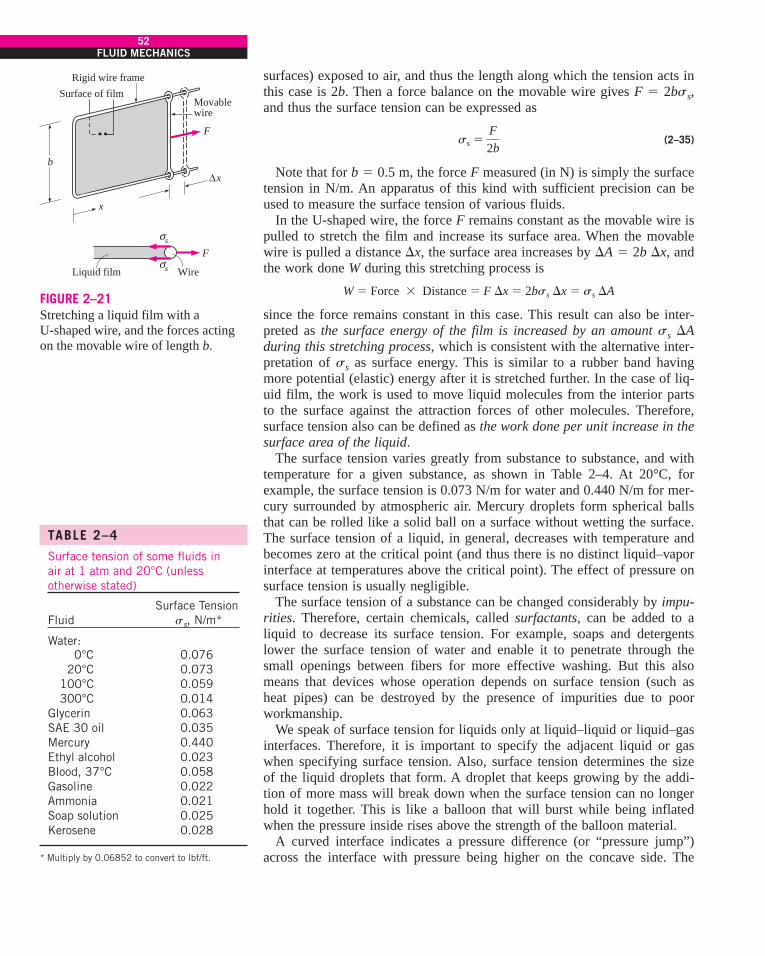
surfaces) exposed to air, and thus the length along which the tension acts inthis case is 2b. Then a force balance on the movable wire gives F ! 2bss,and thus the surface tension can be expressed as

(2–35)

Note that for b ! 0.5 m, the force F measured (in N) is simply the surfacetension in N/m. An apparatus of this kind with sufficient precision can beused to measure the surface tension of various fluids.

In the U-shaped wire, the force F remains constant as the movable wire ispulled to stretch the film and increase its surface area. When the movablewire is pulled a distance &x, the surface area increases by &A ! 2b &x, andthe work done W during this stretching process is

since the force remains constant in this case. This result can also be inter-preted as the surface energy of the film is increased by an amount ss &Aduring this stretching process, which is consistent with the alternative inter-pretation of ss as surface energy. This is similar to a rubber band havingmore potential (elastic) energy after it is stretched further. In the case of liq-uid film, the work is used to move liquid molecules from the interior partsto the surface against the attraction forces of other molecules. Therefore,surface tension also can be defined as the work done per unit increase in thesurface area of the liquid.

The surface tension varies greatly from substance to substance, and withtemperature for a given substance, as shown in Table 2–4. At 20°C, forexample, the surface tension is 0.073 N/m for water and 0.440 N/m for mer-cury surrounded by atmospheric air. Mercury droplets form spherical ballsthat can be rolled like a solid ball on a surface without wetting the surface.The surface tension of a liquid, in general, decreases with temperature andbecomes zero at the critical point (and thus there is no distinct liquid–vaporinterface at temperatures above the critical point). The effect of pressure onsurface tension is usually negligible.

The surface tension of a substance can be changed considerably by impu-rities. Therefore, certain chemicals, called surfactants, can be added to aliquid to decrease its surface tension. For example, soaps and detergentslower the surface tension of water and enable it to penetrate through thesmall openings between fibers for more effective washing. But this alsomeans that devices whose operation depends on surface tension (such asheat pipes) can be destroyed by the presence of impurities due to poorworkmanship.

We speak of surface tension for liquids only at liquid–liquid or liquid–gasinterfaces. Therefore, it is important to specify the adjacent liquid or gaswhen specifying surface tension. Also, surface tension determines the sizeof the liquid droplets that form. A droplet that keeps growing by the addi-tion of more mass will break down when the surface tension can no longerhold it together. This is like a balloon that will burst while being inflatedwhen the pressure inside rises above the strength of the balloon material.

A curved interface indicates a pressure difference (or “pressure jump”)across the interface with pressure being higher on the concave side. The

W ! Force " Distance ! F &x ! 2bss &x ! ss &A

ss !F2b

52FLUID MECHANICS

&x

F

F

Movablewire

Rigid wire frame

Liquid film Wire

Surface of film

b

x

'

'

s

s

FIGURE 2–21Stretching a liquid film with a U-shaped wire, and the forces actingon the movable wire of length b.

TABLE 2–4Surface tension of some fluids in air at 1 atm and 20°C (unlessotherwise stated)

Surface TensionFluid ss, N/m*

Water:0°C 0.076

20°C 0.073100°C 0.059300°C 0.014

Glycerin 0.063SAE 30 oil 0.035Mercury 0.440Ethyl alcohol 0.023Blood, 37°C 0.058Gasoline 0.022Ammonia 0.021Soap solution 0.025Kerosene 0.028

* Multiply by 0.06852 to convert to lbf/ft.

cen72367_ch02.qxd 10/29/04 2:20 PM Page 52

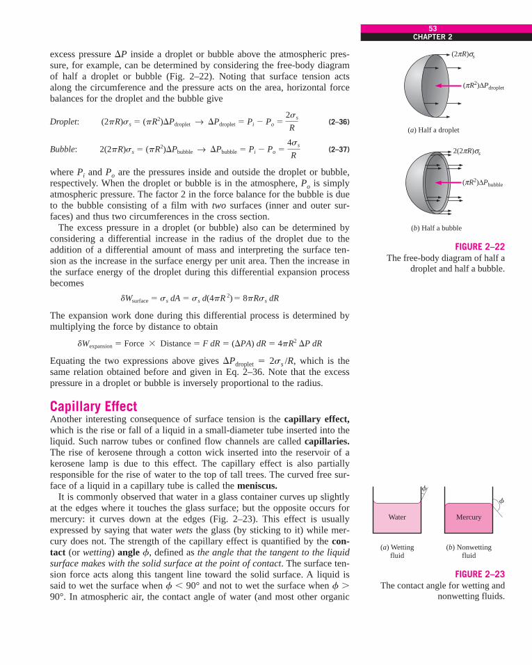
excess pressure &P inside a droplet or bubble above the atmospheric pres-sure, for example, can be determined by considering the free-body diagramof half a droplet or bubble (Fig. 2–22). Noting that surface tension actsalong the circumference and the pressure acts on the area, horizontal forcebalances for the droplet and the bubble give

Droplet: (2–36)

Bubble: (2–37)

where Pi and Po are the pressures inside and outside the droplet or bubble,respectively. When the droplet or bubble is in the atmosphere, Po is simplyatmospheric pressure. The factor 2 in the force balance for the bubble is dueto the bubble consisting of a film with two surfaces (inner and outer sur-faces) and thus two circumferences in the cross section.

The excess pressure in a droplet (or bubble) also can be determined byconsidering a differential increase in the radius of the droplet due to theaddition of a differential amount of mass and interpreting the surface ten-sion as the increase in the surface energy per unit area. Then the increase inthe surface energy of the droplet during this differential expansion processbecomes

The expansion work done during this differential process is determined bymultiplying the force by distance to obtain

Equating the two expressions above gives &Pdroplet ! 2ss /R, which is thesame relation obtained before and given in Eq. 2–36. Note that the excesspressure in a droplet or bubble is inversely proportional to the radius.

Capillary EffectAnother interesting consequence of surface tension is the capillary effect,which is the rise or fall of a liquid in a small-diameter tube inserted into theliquid. Such narrow tubes or confined flow channels are called capillaries.The rise of kerosene through a cotton wick inserted into the reservoir of akerosene lamp is due to this effect. The capillary effect is also partiallyresponsible for the rise of water to the top of tall trees. The curved free sur-face of a liquid in a capillary tube is called the meniscus.

It is commonly observed that water in a glass container curves up slightlyat the edges where it touches the glass surface; but the opposite occurs formercury: it curves down at the edges (Fig. 2–23). This effect is usuallyexpressed by saying that water wets the glass (by sticking to it) while mer-cury does not. The strength of the capillary effect is quantified by the con-tact (or wetting) angle f, defined as the angle that the tangent to the liquidsurface makes with the solid surface at the point of contact. The surface ten-sion force acts along this tangent line toward the solid surface. A liquid issaid to wet the surface when f + 90° and not to wet the surface when f -90°. In atmospheric air, the contact angle of water (and most other organic

dWexpansion ! Force " Distance ! F dR ! (&PA) dR ! 4pR2 &P dR

dWsurface ! ss dA ! ss d(4pR 2)! 8pRss dR

2(2pR)ss ! (pR2)&Pbubble ( &Pbubble ! Pi # Po !4ss

R

(2pR)ss ! (pR2)&Pdroplet ( &Pdroplet ! Pi # Po !2ss

R

53CHAPTER 2

(a) Half a droplet

(2 R) s) '

( R2)&Pdroplet)

(b) Half a bubble

2(2 R) s

( R2)&Pbubble

')

)

FIGURE 2–22The free-body diagram of half a

droplet and half a bubble.

(a) Wettingfluid

Water

(b) Nonwettingfluid

Mercury

f

f

FIGURE 2–23The contact angle for wetting and

nonwetting fluids.

cen72367_ch02.qxd 10/29/04 2:20 PM Page 53

liquids) with glass is nearly zero, f " 0° (Fig. 2–24). Therefore, the surfacetension force acts upward on water in a glass tube along the circumference,tending to pull the water up. As a result, water rises in the tube until theweight of the liquid in the tube above the liquid level of the reservoir bal-ances the surface tension force. The contact angle is 130° for mercury–glassand 26° for kerosene–glass in air. Note that the contact angle, in general, isdifferent in different environments (such as another gas or liquid in place ofair).

The phenomenon of capillary effect can be explained microscopically byconsidering cohesive forces (the forces between like molecules, such aswater and water) and adhesive forces (the forces between unlike molecules,such as water and glass). The liquid molecules at the solid–liquid interfaceare subjected to both cohesive forces by other liquid molecules and adhesiveforces by the molecules of the solid. The relative magnitudes of these forcesdetermine whether a liquid wets a solid surface or not. Obviously, the watermolecules are more strongly attracted to the glass molecules than they are toother water molecules, and thus water tends to rise along the glass surface.The opposite occurs for mercury, which causes the liquid surface near theglass wall to be suppressed (Fig. 2–25).

The magnitude of the capillary rise in a circular tube can be determinedfrom a force balance on the cylindrical liquid column of height h in the tube(Fig. 2–26). The bottom of the liquid column is at the same level as the freesurface of the reservoir, and thus the pressure there must be atmosphericpressure. This balances the atmospheric pressure acting at the top surface,and thus these two effects cancel each other. The weight of the liquid col-umn is approximately

Equating the vertical component of the surface tension force to the weightgives

Solving for h gives the capillary rise to be

Capillary rise: (2–38)

This relation is also valid for nonwetting liquids (such as mercury in glass)and gives the capillary drop. In this case f - 90° and thus cos f + 0,which makes h negative. Therefore, a negative value of capillary rise corre-sponds to a capillary drop (Fig. 2–25).

Note that the capillary rise is inversely proportional to the radius of thetube. Therefore, the thinner the tube is, the greater the rise (or fall) of theliquid in the tube. In practice, the capillary effect is usually negligible intubes whose diameter is greater than 1 cm. When pressure measurementsare made using manometers and barometers, it is important to use suffi-ciently large tubes to minimize the capillary effect. The capillary rise is alsoinversely proportional to the density of the liquid, as expected. Therefore,lighter liquids experience greater capillary rises. Finally, it should be kept inmind that Eq. 2–38 is derived for constant-diameter tubes and should not beused for tubes of variable cross section.

h !2ss

rgR cos f (R ! constant)

W ! Fsurface ( rg(pR2h) ! 2pRss cos f

W ! mg ! rVg ! rg(pR2h)

54FLUID MECHANICS

FIGURE 2–24The meniscus of colored water in a 4-mm-inner-diameter glass tube. Notethat the edge of the meniscus meetsthe wall of the capillary tube at a verysmall contact angle.Photo by Gabrielle Trembley, Pennsylvania StateUniversity. Used by permission.

Meniscus

Water Mercury

h > 0

h < 0

Meniscus

FIGURE 2–25The capillary rise of water and the capillary fall of mercury in asmall-diameter glass tube.

h

W

2R

Liquid

2pRssf

FIGURE 2–26The forces acting on a liquid columnthat has risen in a tube due to thecapillary effect.

cen72367_ch02.qxd 10/29/04 2:20 PM Page 54

EXAMPLE 2–5 The Capillary Rise of Water in a Tube

A 0.6-mm-diameter glass tube is inserted into water at 20°C in a cup. Deter-mine the capillary rise of water in the tube (Fig. 2–27).

SOLUTION The rise of water in a slender tube as a result of the capillaryeffect is to be determined.Assumptions 1 There are no impurities in the water and no contaminationon the surfaces of the glass tube. 2 The experiment is conducted in atmos-pheric air.Properties The surface tension of water at 20°C is 0.073 N/m (Table 2–3).The contact angle of water with glass is 0° (from preceding text). We takethe density of liquid water to be 1000 kg/m3.Analysis The capillary rise is determined directly from Eq. 2–15 by substi-tuting the given values, yielding

Therefore, water rises in the tube 5 cm above the liquid level in the cup.Discussion Note that if the tube diameter were 1 cm, the capillary risewould be 0.3 mm, which is hardly noticeable to the eye. Actually, the capil-lary rise in a large-diameter tube occurs only at the rim. The center does notrise at all. Therefore, the capillary effect can be ignored for large-diametertubes.

! 0.050 m ! 5.0 cm

h !2ss

rgR cos f !

2(0.073 N/m)(1000 kg/m3)(9.81 m/s2)(0.3 " 10#3m)

(cos 0$)a1kg , m/s2

1 Nb

55CHAPTER 2

SUMMARY

In this chapter various properties commonly used in fluidmechanics are discussed. The mass-dependent properties of asystem are called extensive properties and the others, inten-sive properties. Density is mass per unit volume, and specificvolume is volume per unit mass. The specific gravity isdefined as the ratio of the density of a substance to the den-sity of water at 4°C,

The ideal-gas equation of state is expressed as

where P is the absolute pressure, T is the thermodynamictemperature, r is the density, and R is the gas constant.

At a given temperature, the pressure at which a pure sub-stance changes phase is called the saturation pressure. Forphase-change processes between the liquid and vapor phasesof a pure substance, the saturation pressure is commonlycalled the vapor pressure Pv. Vapor bubbles that form in the

P ! rRT

SG !r

rH2O

low-pressure regions in a liquid (a phenomenon called cavita-tion) collapse as they are swept away from the low-pressureregions, generating highly destructive, extremely high-pressurewaves.

Energy can exist in numerous forms, and their sum consti-tutes the total energy E (or e on a unit-mass basis) of a sys-tem. The sum of all microscopic forms of energy is called theinternal energy U of a system. The energy that a system pos-sesses as a result of its motion relative to some referenceframe is called kinetic energy expressed per unit mass aske ! V2/2, and the energy that a system possesses as a resultof its elevation in a gravitational field is called potentialenergy expressed per unit mass as pe ! gz.

The compressibility effects in a fluid are represented by thecoefficient of compressibility k (also called bulk modulusof elasticity) defined as

k ! #v a'P'vb

T! ra'P

'rb

T ! #

&P&v/v

h

WWater

Air

2pRss cos f

FIGURE 2–27Schematic for Example 2–5.

cen72367_ch02.qxd 10/29/04 2:20 PM Page 55

56FLUID MECHANICS

REFERENCES AND SUGGESTED READING

1. E. C. Bingham. “An Investigation of the Laws of PlasticFlow,” U.S. Bureau of Standards Bulletin, 13, pp.309–353, 1916.

2. Y. A. Cengel and M. A. Boles. Thermodynamics: AnEngineering Approach, 4th ed. New York: McGraw-Hill,2002.

3. C. T. Crowe, J. A. Roberson, and D. F. Elger. EngineeringFluid Mechanics, 7th ed. New York: Wiley, 2001.

4. R. W. Fox and A. T. McDonald. Introduction to FluidMechanics, 5th ed. New York: Wiley, 1999.

5. D. C. Giancoli. Physics, 3rd ed. Upper Saddle River, NJ:Prentice Hall, 1991.

6. M. C. Potter and D. C. Wiggert. Mechanics of Fluids, 2nded. Upper Saddle River, NJ: Prentice Hall, 1997.

7. Y. S. Touloukian, S. C. Saxena, and P. Hestermans.Thermophysical Properties of Matter, The TPRC DataSeries, Vol. 11, Viscosity. New York: Plenum, 1975.

8. L. Trefethen. “Surface Tension in Fluid Mechanics.” InIllustrated Experiments in Fluid Mechanics. Cambridge,MA: MIT Press, 1972.

9. The U.S. Standard Atmosphere. Washington, DC: U.S.Government Printing Office, 1976.

10. M. Van Dyke. An Album of Fluid Motion. Stanford, CA:Parabolic Press, 1982.

11. F. M. White. Fluid Mechanics, 5th ed. New York:McGraw-Hill, 2003.

12. C. L. Yaws, X. Lin, and L. Bu. “Calculate Viscosities for355 Compounds. An Equation Can Be Used to CalculateLiquid Viscosity as a Function of Temperature,” ChemicalEngineering, 101, no. 4, pp. 1110–1128, April 1994.

13. C. L. Yaws. Handbook of Viscosity. 3 Vols. Houston, TX:Gulf Publishing, 1994.

The property that represents the variation of the density ofa fluid with temperature at constant pressure is the volumeexpansion coefficient (or volume expansivity) b, defined as

The viscosity of a fluid is a measure of its resistance todeformation. The tangential force per unit area is called shearstress and is expressed for simple shear flow between plates(one-dimensional flow) as

where m is the coefficient of viscosity or the dynamic (orabsolute) viscosity of the fluid, u is the velocity component inthe flow direction, and y is the direction normal to the flowdirection. The fluids that obey this linear relationship are calledNewtonian fluids. The ratio of dynamic viscosity to density iscalled the kinematic viscosity n.

The pulling effect on the liquid molecules at an interfacecaused by the attractive forces of molecules per unit length iscalled surface tension ss. The excess pressure &P inside aspherical droplet or bubble is given by

&Pdroplet ! Pi # Po !2ss

R and &Pbubble ! Pi # Po !

4ss

R

t ! m dudy

b !1v a'v

'Tb

P! #

1ra'r'Tb

P ! #

&r/r&T

where Pi and Po are the pressures inside and outside thedroplet or bubble. The rise or fall of a liquid in a small-diametertube inserted into the liquid due to surface tension is calledthe capillary effect. The capillary rise or drop is given by

where f is the contact angle. The capillary rise is inverselyproportional to the radius of the tube and is negligible fortubes whose diameter is larger than about 1 cm.

Density and viscosity are two of the most fundamentalproperties of fluids, and they are used extensively in thechapters that follow. In Chap. 3, the effect of density on thevariation of pressure in a fluid is considered, and the hydro-static forces acting on surfaces are determined. In Chap. 8,the pressure drop caused by viscous effects during flow iscalculated and used in the determination of the pumpingpower requirements. Viscosity is also used as a key propertyin the formulation and solutions of the equations of fluidmotion in Chaps. 9 and 10.

h !2ss

rgR cos f

cen72367_ch02.qxd 10/29/04 2:20 PM Page 56

CHAPTER 25757

CHAPTER 2

(a)

(b)

FIGURE 2–28(a) Vaporous cavitation occurs in

water that has very little entrained gas, such as that found very deep in a body of water. Cavitation bubbles

are formed when the speed of thebody—in this case the bulbulous bowregion of a surface ship sonar dome—increases to the point where the local

static pressure falls below the vaporpressure of the water. The cavitation

bubbles are filled essentially withwater vapor. This type of cavitation is very violent and noisy. (b) On the

other hand, in shallow water, there ismuch more entrained gas in the water

to act as cavitation nuclei. That’sbecause of the proximity of the dometo the atmosphere at the free surface.The cavitation bubbles first appear at a slower speed, and hence at a higher

local static pressure. They arepredominantly filled with the gases

that are entrained in the water, so thisis known as gaseous cavitation.Reprinted by permission of G. C. Lauchle

and M. L. Billet, Penn State University.

Guest Authors: G. C. Lauchle and M. L. Billet,Penn State University

Cavitation is the rupture of a liquid, or of a fluid–solid interface, caused by areduction of the local static pressure produced by the dynamic action of thefluid in the interior and/or boundaries of a liquid system. The rupture is theformation of a visible bubble. Liquids, such as water, contain many micro-scopic voids that act as cavitation nuclei. Cavitation occurs when thesenuclei grow to a significant, visible size. Although boiling is also the forma-tion of voids in a liquid, we usually separate this phenomenon from cavita-tion because it is caused by an increase in temperature, rather than by areduction in pressure. Cavitation can be used in beneficial ways, such as inultrasonic cleaners, etchers, and cutters. But more often than not, cavitationis to be avoided in fluid flow applications because it spoils hydrodynamicperformance, it causes extremely loud noise and high vibration levels, and itdamages (erodes) the surfaces that support it. When cavitation bubbles enterregions of high pressure and collapse, the underwater shock waves some-times create minute amounts of light. This phenomenon is called sonolumi-nescence.

Body cavitation is illustrated in Fig. 2–28. The body is a model of the under-water bulbulous bow region of a surface ship. It is shaped this way becauselocated within it is a sound navigation and ranging (sonar) system that isspherical in shape. This part of the surface ship is thus called a sonar dome. Asship speeds get faster and faster some of these domes start to cavitate and thenoise created by the cavitation renders the sonar system useless. Naval archi-tects and fluid dynamicists attempt to design these domes so that they will notcavitate. Model-scale testing allows the engineer to see first hand whether agiven design provides improved cavitation performance. Because such tests areconducted in water tunnels, the conditions of the test water should have suffi-cient nuclei to model those conditions in which the prototype operates. Thisassures that the effect of liquid tension (nuclei distribution) is minimized.Important variables are the gas content level (nuclei distribution) of the water,the temperature, and the hydrostatic pressure at which the body operates. Cavi-tation first appears—as either the speed V is increased, or as the submergencedepth h is decreased—at the minimum pressure point Cpmin

of the body. Thus,good hydrodynamic design requires 2(P( # Pv)/rV2 - Cpmin

, where r is den-sity, P( ! rgh is the reference to static pressure, Cp is the pressure coefficient(Chap. 7), and Pv is the vapor pressure of water.

ReferencesLauchle, G. C., Billet, M. L., and Deutsch, S., “High-Reynolds Number Liquid

Flow Measurements,” in Lecture Notes in Engineering, Vol. 46, Frontiers inExperimental Fluid Mechanics, Springer-Verlag, Berlin, edited by M. Gad-el-Hak, Chap. 3, pp. 95–158, 1989.

Ross, D., Mechanics of Underwater Noise, Peninsula Publ., Los Altos, CA, 1987.Barber, B. P., Hiller, R. A., Löfstedt, R., Putterman, S. J., and Weninger, K. R.,

“Defining the Unknowns of Sonoluminescence,” Physics Reports, Vol. 281, pp.65–143, 1997.

APPLICATION SPOTLIGHT ! Cavitation

cen72367_ch02.qxd 10/29/04 2:20 PM Page 57

58FLUID MECHANICS

PROBLEMS*

Density and Specific Gravity2–1C What is the difference between intensive and exten-sive properties?

2–2C What is specific gravity? How is it related to density?

2–3C Under what conditions is the ideal-gas assumptionsuitable for real gases?

2–4C What is the difference between R and Ru? How arethese two related?

2–5 A spherical balloon with a diameter of 6 m is filledwith helium at 20°C and 200 kPa. Determine the mole num-ber and the mass of the helium in the balloon. Answers: 9.28kmol, 37.2 kg

2–6 Reconsider Prob. 2–5. Using EES (or other) soft-ware, investigate the effect of the balloon diame-

ter on the mass of helium contained in the balloon for thepressures of (a) 100 kPa and (b) 200 kPa. Let the diametervary from 5 m to 15 m. Plot the mass of helium against thediameter for both cases.

2–7 The pressure in an automobile tire depends on the tem-perature of the air in the tire. When the air temperature is25°C, the pressure gage reads 210 kPa. If the volume of thetire is 0.025 m3, determine the pressure rise in the tire whenthe air temperature in the tire rises to 50°C. Also, determinethe amount of air that must be bled off to restore pressure toits original value at this temperature. Assume the atmosphericpressure to be 100 kPa.

2–8E The air in an automobile tire with a volume of 0.53ft3 is at 90°F and 20 psig. Determine the amount of air thatmust be added to raise the pressure to the recommendedvalue of 30 psig. Assume the atmospheric pressure to be 14.6psia and the temperature and the volume to remain constant.Answer: 0.0260 lbm

2–9E A rigid tank contains 20 lbm of air at 20 psia and70°F. More air is added to the tank until the pressure andtemperature rise to 35 psia and 90°F, respectively. Determinethe amount of air added to the tank. Answer: 13.7 lbm

2–10 The density of atmospheric air varies with eleva-tion, decreasing with increasing altitude. (a)

Using the data given in the table, obtain a relation for thevariation of density with elevation, and calculate the densityat an elevation of 7000 m. (b) Calculate the mass of theatmosphere using the correlation you obtained. Assume theearth to be a perfect sphere with a radius of 6377 km, andtake the thickness of the atmosphere to be 25 km.

z, km r, kg/m3

6377 1.2256378 1.1126379 1.0076380 0.90936381 0.81946382 0.73646383 0.66016385 0.52586387 0.41356392 0.19486397 0.088916402 0.04008

Vapor Pressure and Cavitation2–11C What is vapor pressure? How is it related to satura-tion pressure?

2–12C Does water boil at higher temperatures at higherpressures? Explain.

2–13C If the pressure of a substance is increased during aboiling process, will the temperature also increase or will itremain constant? Why?

2–14C What is cavitation? What causes it?

2–15 In a piping system, the water temperature remainsunder 40°C. Determine the minimum pressure allowed in thesystem to avoid cavitation.

2–16 The analysis of a propeller that operates in water at20°C shows that the pressure at the tips of the propeller dropsto 2 kPa at high speeds. Determine if there is a danger of cav-itation for this propeller.

AIR

V = 0.025 m3

T = 25°CPg = 210 kPa

FIGURE P2–7

* Problems designated by a “C” are concept questions, andstudents are encouraged to answer them all. Problems designatedby an “E” are in English units, and the SI users can ignore them.Problems with the icon are solved using EES, and completesolutions together with parametric studies are included on theenclosed DVD. Problems with the icon are comprehensive innature and are intended to be solved with a computer, preferablyusing the EES software that accompanies this text.

cen72367_ch02.qxd 11/16/04 11:34 AM Page 58

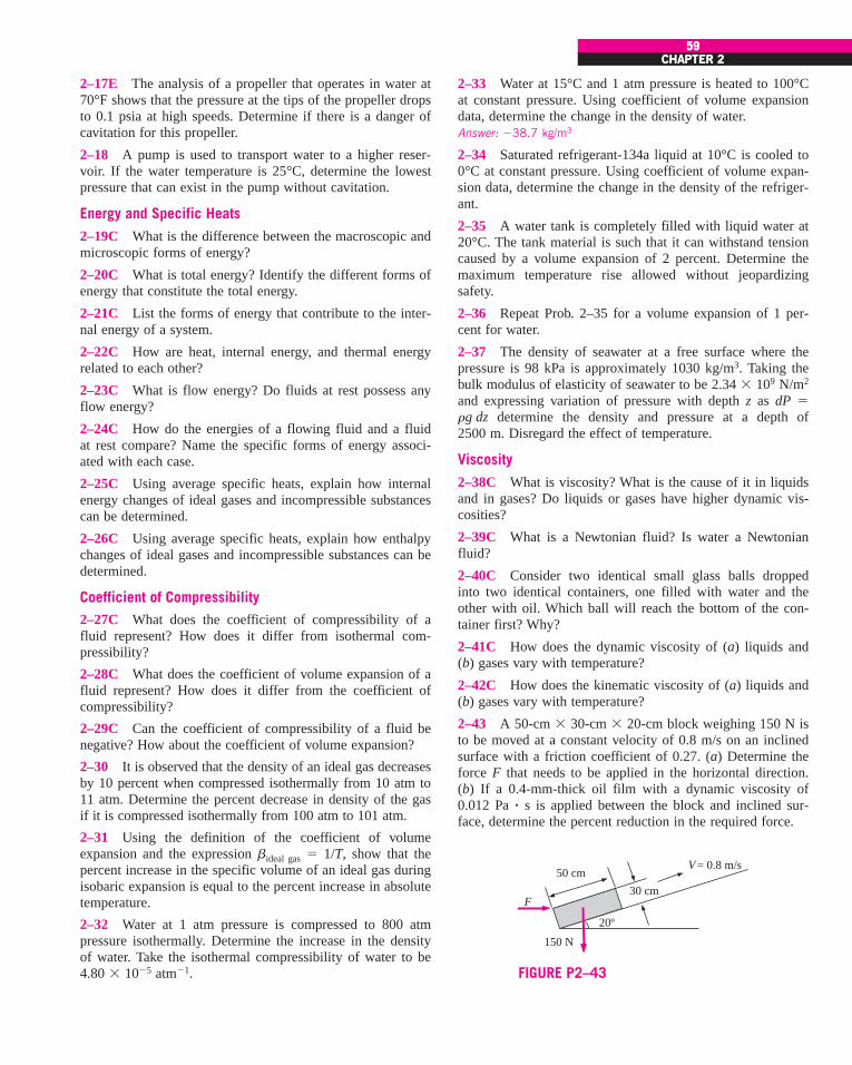
CHAPTER 259

2–17E The analysis of a propeller that operates in water at70°F shows that the pressure at the tips of the propeller dropsto 0.1 psia at high speeds. Determine if there is a danger ofcavitation for this propeller.

2–18 A pump is used to transport water to a higher reser-voir. If the water temperature is 25°C, determine the lowestpressure that can exist in the pump without cavitation.

Energy and Specific Heats2–19C What is the difference between the macroscopic andmicroscopic forms of energy?

2–20C What is total energy? Identify the different forms ofenergy that constitute the total energy.

2–21C List the forms of energy that contribute to the inter-nal energy of a system.

2–22C How are heat, internal energy, and thermal energyrelated to each other?

2–23C What is flow energy? Do fluids at rest possess anyflow energy?

2–24C How do the energies of a flowing fluid and a fluidat rest compare? Name the specific forms of energy associ-ated with each case.

2–25C Using average specific heats, explain how internalenergy changes of ideal gases and incompressible substancescan be determined.

2–26C Using average specific heats, explain how enthalpychanges of ideal gases and incompressible substances can bedetermined.

Coefficient of Compressibility2–27C What does the coefficient of compressibility of afluid represent? How does it differ from isothermal com-pressibility?

2–28C What does the coefficient of volume expansion of afluid represent? How does it differ from the coefficient ofcompressibility?

2–29C Can the coefficient of compressibility of a fluid benegative? How about the coefficient of volume expansion?

2–30 It is observed that the density of an ideal gas decreasesby 10 percent when compressed isothermally from 10 atm to11 atm. Determine the percent decrease in density of the gasif it is compressed isothermally from 100 atm to 101 atm.

2–31 Using the definition of the coefficient of volumeexpansion and the expression bideal gas ! 1/T, show that thepercent increase in the specific volume of an ideal gas duringisobaric expansion is equal to the percent increase in absolutetemperature.

2–32 Water at 1 atm pressure is compressed to 800 atmpressure isothermally. Determine the increase in the densityof water. Take the isothermal compressibility of water to be4.80 " 10#5 atm#1.

2–33 Water at 15°C and 1 atm pressure is heated to 100°Cat constant pressure. Using coefficient of volume expansiondata, determine the change in the density of water.Answer: #38.7 kg/m3

2–34 Saturated refrigerant-134a liquid at 10°C is cooled to0°C at constant pressure. Using coefficient of volume expan-sion data, determine the change in the density of the refriger-ant.

2–35 A water tank is completely filled with liquid water at20°C. The tank material is such that it can withstand tensioncaused by a volume expansion of 2 percent. Determine themaximum temperature rise allowed without jeopardizingsafety.

2–36 Repeat Prob. 2–35 for a volume expansion of 1 per-cent for water.

2–37 The density of seawater at a free surface where thepressure is 98 kPa is approximately 1030 kg/m3. Taking thebulk modulus of elasticity of seawater to be 2.34 " 109 N/m2

and expressing variation of pressure with depth z as dP !rg dz determine the density and pressure at a depth of2500 m. Disregard the effect of temperature.

Viscosity2–38C What is viscosity? What is the cause of it in liquidsand in gases? Do liquids or gases have higher dynamic vis-cosities?

2–39C What is a Newtonian fluid? Is water a Newtonianfluid?

2–40C Consider two identical small glass balls droppedinto two identical containers, one filled with water and theother with oil. Which ball will reach the bottom of the con-tainer first? Why?

2–41C How does the dynamic viscosity of (a) liquids and(b) gases vary with temperature?

2–42C How does the kinematic viscosity of (a) liquids and(b) gases vary with temperature?

2–43 A 50-cm " 30-cm " 20-cm block weighing 150 N isto be moved at a constant velocity of 0.8 m/s on an inclinedsurface with a friction coefficient of 0.27. (a) Determine theforce F that needs to be applied in the horizontal direction.(b) If a 0.4-mm-thick oil film with a dynamic viscosity of0.012 Pa ! s is applied between the block and inclined sur-face, determine the percent reduction in the required force.

59CHAPTER 2

150 N

F

= 0.8 m/s

30 cm

50 cm

20º

V

FIGURE P2–43

cen72367_ch02.qxd 10/29/04 2:20 PM Page 59

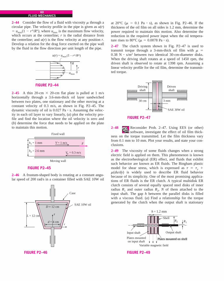
2–44 Consider the flow of a fluid with viscosity m through acircular pipe. The velocity profile in the pipe is given as u(r)! umax(1 # rn/Rn), where umax is the maximum flow velocity,which occurs at the centerline; r is the radial distance fromthe centerline; and u(r) is the flow velocity at any position r.Develop a relation for the drag force exerted on the pipe wallby the fluid in the flow direction per unit length of the pipe.

60FLUID MECHANICS

at 20°C (m ! 0.1 Pa ! s), as shown in Fig. P2–46. If thethickness of the oil film on all sides is 1.2 mm, determine thepower required to maintain this motion. Also determine thereduction in the required power input when the oil tempera-ture rises to 80°C (m ! 0.0078 Pa ! s).

2–47 The clutch system shown in Fig. P2–47 is used totransmit torque through a 3-mm-thick oil film with m !0.38 N ! s/m2 between two identical 30-cm-diameter disks.When the driving shaft rotates at a speed of 1450 rpm, thedriven shaft is observed to rotate at 1398 rpm. Assuming alinear velocity profile for the oil film, determine the transmit-ted torque.

2–45 A thin 20-cm " 20-cm flat plate is pulled at 1 m/shorizontally through a 3.6-mm-thick oil layer sandwichedbetween two plates, one stationary and the other moving at aconstant velocity of 0.3 m/s, as shown in Fig. P2–45. Thedynamic viscosity of oil is 0.027 Pa ! s. Assuming the veloc-ity in each oil layer to vary linearly, (a) plot the velocity pro-file and find the location where the oil velocity is zero and(b) determine the force that needs to be applied on the plateto maintain this motion.

rR

umax

u(r) = umax(1 – rn/Rn)

0

FIGURE P2–44

2–46 A frustum-shaped body is rotating at a constant angu-lar speed of 200 rad/s in a container filled with SAE 10W oil

F

Fixed wall

Moving wall

= 1 m/sh1 = 1 mm

h2 = 2.6 mm w = 0.3 m/s

V

V

FIGURE P2–45

D = 12 cm

L = 12 cm

d = 4 cm

Case

SAE 10W oil

r

z

FIGURE P2–46

2–48 Reconsider Prob. 2–47. Using EES (or other)software, investigate the effect of oil film thick-

ness on the torque transmitted. Let the film thickness varyfrom 0.1 mm to 10 mm. Plot your results, and state your con-clusions.

2–49 The viscosity of some fluids changes when a strongelectric field is applied on them. This phenomenon is knownas the electrorheological (ER) effect, and fluids that exhibitsuch behavior are known as ER fluids. The Bingham plasticmodel for shear stress, which is expressed as t ! ty %m(du/dy) is widely used to describe ER fluid behaviorbecause of its simplicity. One of the most promising applica-tions of ER fluids is the ER clutch. A typical multidisk ERclutch consists of several equally spaced steel disks of innerradius R1 and outer radius R2, N of them attached to theinput shaft. The gap h between the parallel disks is filledwith a viscous fluid. (a) Find a relationship for the torquegenerated by the clutch when the output shaft is stationary

30 cm

Drivingshaft

Drivenshaft

SAE 30W oil

3 mm

FIGURE P2–47

Shell

Input shaft

Plates mountedon input shaft

Variable magnetic field

Output shaft

R2 R1

Plates mounted on shellPlates mounted on shell

h = 1.2 mm

FIGURE P2–49

cen72367_ch02.qxd 10/29/04 2:20 PM Page 60

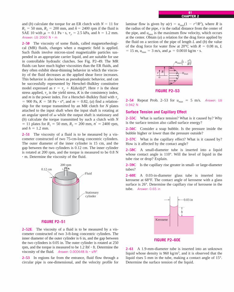
CHAPTER 261

and (b) calculate the torque for an ER clutch with N ! 11 forR1 ! 50 mm, R2 ! 200 mm, and n

.! 2400 rpm if the fluid is

SAE 10 with m ! 0.1 Pa ! s, ty ! 2.5 kPa, and h ! 1.2 mm.Answer: (b) 2060 N ! m

2–50 The viscosity of some fluids, called magnetorheologi-cal (MR) fluids, changes when a magnetic field is applied.Such fluids involve micron-sized magnetizable particles sus-pended in an appropriate carrier liquid, and are suitable for usein controllable hydraulic clutches. See Fig. P2–49. The MRfluids can have much higher viscosities than the ER fluids, andthey often exhibit shear-thinning behavior in which the viscos-ity of the fluid decreases as the applied shear force increases.This behavior is also known as pseudoplastic behavior, and canbe successfully represented by Herschel–Bulkley constitutivemodel expressed as t ! ty % K(du/dy)m. Here t is the shearstress applied, ty is the yield stress, K is the consistency index,and m is the power index. For a Herschel–Bulkley fluid with ty! 900 Pa, K ! 58 Pa ! sm, and m ! 0.82, (a) find a relation-ship for the torque transmitted by an MR clutch for N platesattached to the input shaft when the input shaft is rotating atan angular speed of v while the output shaft is stationary and(b) calculate the torque transmitted by such a clutch with N! 11 plates for R1 ! 50 mm, R2 ! 200 mm, n

.! 2400 rpm,

and h ! 1.2 mm.

2–51 The viscosity of a fluid is to be measured by a vis-cometer constructed of two 75-cm-long concentric cylinders.The outer diameter of the inner cylinder is 15 cm, and thegap between the two cylinders is 0.12 cm. The inner cylinderis rotated at 200 rpm, and the torque is measured to be 0.8 N! m. Determine the viscosity of the fluid.

2–54 Repeat Prob. 2–53 for umax ! 5 m/s. Answer: (b)0.942 N

Surface Tension and Capillary Effect2–55C What is surface tension? What is it caused by? Whyis the surface tension also called surface energy?

2–56C Consider a soap bubble. Is the pressure inside thebubble higher or lower than the pressure outside?

2–57C What is the capillary effect? What is it caused by?How is it affected by the contact angle?

2–58C A small-diameter tube is inserted into a liquidwhose contact angle is 110°. Will the level of liquid in thetube rise or drop? Explain.

2–59C Is the capillary rise greater in small- or large-diametertubes?

2–60E A 0.03-in-diameter glass tube is inserted intokerosene at 68°F. The contact angle of kerosene with a glasssurface is 26°. Determine the capillary rise of kerosene in thetube. Answer: 0.65 in

61CHAPTER 2

2–52E The viscosity of a fluid is to be measured by a vis-cometer constructed of two 3-ft-long concentric cylinders. Theinner diameter of the outer cylinder is 6 in, and the gap betweenthe two cylinders is 0.05 in. The outer cylinder is rotated at 250rpm, and the torque is measured to be 1.2 lbf ! ft. Determine theviscosity of the fluid. Answer: 0.000648 lb ! s/ft2

2–53 In regions far from the entrance, fluid flow through acircular pipe is one-dimensional, and the velocity profile for

0.12 cmFluid

200 rpm

Stationarycylinder

FIGURE P2–51

r R umax

umax( )1 – r2

R2

o

FIGURE P2–53

2–61 A 1.9-mm-diameter tube is inserted into an unknownliquid whose density is 960 kg/m3, and it is observed that theliquid rises 5 mm in the tube, making a contact angle of 15°.Determine the surface tension of the liquid.

h

0.03 in

Kerosene

FIGURE P2–60E

laminar flow is given by u(r) ! umax(1 # r2/R2), where R isthe radius of the pipe, r is the radial distance from the center ofthe pipe, and umax is the maximum flow velocity, which occursat the center. Obtain (a) a relation for the drag force applied bythe fluid on a section of the pipe of length L and (b) the valueof the drag force for water flow at 20°C with R ! 0.08 m, L! 15 m, umax ! 3 m/s, and m ! 0.0010 kg/m ! s.

cen72367_ch02.qxd 10/29/04 2:20 PM Page 61

2–62 Determine the gage pressure inside a soap bub-ble of diameter (a) 0.2 cm and (b) 5 cm at 20°C.

2–63 Nutrients dissolved in water are carried to upper partsof plants by tiny tubes partly because of the capillary effect.Determine how high the water solution will rise in a tree in a0.005-mm-diameter tube as a result of the capillary effect.Treat the solution as water at 20°C with a contact angle of15°. Answer: 5.75 m

62FLUID MECHANICS

cles either by weight or mass Cs, mass ! ms /mm or by volume,Cs, vol ! Vs /Vm where m is mass and V is volume. The sub-scripts s and m indicate solid and mixture, respectively.Develop an expression for the specific gravity of a water-based suspension in terms of Cs, mass and Cs, vol.

2–69 The specific gravities of solids and carrier fluids of aslurry are usually known, but the specific gravity of the slurrydepends on the concentration of the solid particles. Show thatthe specific gravity of a water-based slurry can be expressedin terms of the specific gravity of the solid SGs and the massconcentration of the suspended solid particles Cs, mass as

2–70E The pressure on the suction side of pumps is typi-cally low, and the surfaces on that side of the pump are sus-ceptible to cavitation, especially at high fluid temperatures. Ifthe minimum pressure on the suction side of a water pump is0.95 psia absolute, determine the maximum water tempera-ture to avoid the danger of cavitation.

2–71 A closed tank is partially filled with water at 60°C. Ifthe air above the water is completely evacuated, determinethe absolute pressure in the evacuated space. Assume thetemperature to remain constant.

2–72 The variation of the dynamic viscosity of waterwith absolute temperature is given as

T, K m, Pa ! s

273.15 1.787 " 10#3

278.15 1.519 " 10#3

283.15 1.307 " 10#3

293.15 1.002 " 10#3

303.15 7.975 " 10#4

313.15 6.529 " 10#4

333.15 4.665 " 10#4

353.15 3.547 " 10#4

373.15 2.828 " 10#4

Using tabulated data, develop a relation for viscosity in theform of m ! m(T) ! A % BT % CT 2 % DT 3 % ET 4. Usingthe relation developed, predict the dynamic viscosity of waterat 50°C at which the reported value is 5.468 " 10#4 Pa ! s.Compare your result with the results of Andrade’s equation,which is given in the form of m ! D ! eB/T, where D and Bare constants whose values are to be determined using theviscosity data given.

2–73 Consider laminar flow of a Newtonian fluid of viscos-ity m between two parallel plates. The flow is one-dimen-sional, and the velocity profile is given as u(y) ! 4umax[ y/h # (y/h)2], where y is the vertical coordinate from thebottom surface, h is the distance between the two plates, andumax is the maximum flow velocity that occurs at midplane.

SGm !1

1 % Cs, mass(1/SGs # 1)

2–64 The surface tension of a liquid is to be measured usinga liquid film suspended on a U-shaped wire frame with an8-cm-long movable side. If the force needed to move the wireis 0.012 N, determine the surface tension of this liquid in air.

2–65 Contrary to what you might expect, a solid steel ballcan float on water due to the surface tension effect. Deter-mine the maximum diameter of a steel ball that would floaton water at 20°C. What would your answer be for an alu-minum ball? Take the densities of steel and aluminum ballsto be 7800 kg/m3 and 2700 kg/m3, respectively.

Review Problems2–66 The absolute pressure of an automobile tire is mea-sured to be 290 kPa before a trip and 310 kPa after the trip.Assuming the volume of the tire remains constant at 0.022 m3,determine the percent increase in the absolute temperature ofthe air in the tire.

2–67 A 20-m3 tank contains nitrogen at 25°C and 800 kPa.Some nitrogen is allowed to escape until the pressure in thetank drops to 600 kPa. If the temperature at this point is20°C, determine the amount of nitrogen that has escaped.Answer: 42.9 kg

2–68 The composition of a liquid with suspended solid par-ticles is generally characterized by the fraction of solid parti-

0.005 mmWater solution

FIGURE P2–63

cen72367_ch02.qxd 10/29/04 2:20 PM Page 62

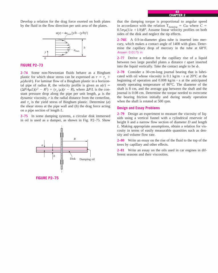
CHAPTER 26363

CHAPTER 2

yh

umax

u(y) = 4umax[y/h – (y/h)2]

0

FIGURE P2–73

that the damping torque is proportional to angular speed in accordance with the relation Tdamping ! Cv where C !0.5pm(1/a %1/b)R4. Assume linear velocity profiles on bothsides of the disk and neglect the tip effects.

2–76E A 0.9-in-diameter glass tube is inserted into mer-cury, which makes a contact angle of 1408 with glass. Deter-mine the capillary drop of mercury in the tube at 68°F.Answer: 0.0175 in

2–77 Derive a relation for the capillary rise of a liquidbetween two large parallel plates a distance t apart insertedinto the liquid vertically. Take the contact angle to be f.

2–78 Consider a 30-cm-long journal bearing that is lubri-cated with oil whose viscosity is 0.1 kg/m ! s at 20°C at thebeginning of operation and 0.008 kg/m ! s at the anticipatedsteady operating temperature of 80°C. The diameter of theshaft is 8 cm, and the average gap between the shaft and thejournal is 0.08 cm. Determine the torque needed to overcomethe bearing friction initially and during steady operationwhen the shaft is rotated at 500 rpm.

Design and Essay Problems2–79 Design an experiment to measure the viscosity of liq-uids using a vertical funnel with a cylindrical reservoir ofheight h and a narrow flow section of diameter D and lengthL. Making appropriate assumptions, obtain a relation for vis-cosity in terms of easily measurable quantities such as den-sity and volume flow rate.

2–80 Write an essay on the rise of the fluid to the top of thetrees by capillary and other effects.

2–81 Write an essay on the oils used in car engines in dif-ferent seasons and their viscosities.

Disk Damping oil

a

b

R

FIGURE P2–75

Develop a relation for the drag force exerted on both platesby the fluid in the flow direction per unit area of the plates.

2–74 Some non-Newtonian fluids behave as a Binghamplastic for which shear stress can be expressed as t ! ty %m(du/dr). For laminar flow of a Bingham plastic in a horizon-tal pipe of radius R, the velocity profile is given as u(r) !(&P/4mL)(r2 # R2) % (ty /m)(r # R), where &P/L is the con-stant pressure drop along the pipe per unit length, m is thedynamic viscosity, r is the radial distance from the centerline,and ty is the yield stress of Bingham plastic. Determine (a)the shear stress at the pipe wall and (b) the drag force actingon a pipe section of length L.

2–75 In some damping systems, a circular disk immersedin oil is used as a damper, as shown in Fig. P2–75. Show

cen72367_ch02.qxd 10/29/04 2:20 PM Page 63

cen72367_ch02.qxd 10/29/04 2:20 PM Page 64

P R E S S U R E A N D F L U I D S TAT I C S

This chapter deals with forces applied by fluids at rest or in rigid-bodymotion. The fluid property responsible for those forces is pressure,which is a normal force exerted by a fluid per unit area. We start this

chapter with a detailed discussion of pressure, including absolute and gagepressures, the pressure at a point, the variation of pressure with depth in agravitational field, the manometer, the barometer, and pressure measure-ment devices. This is followed by a discussion of the hydrostatic forcesapplied on submerged bodies with plane or curved surfaces. We then con-sider the buoyant force applied by fluids on submerged or floating bodies,and discuss the stability of such bodies. Finally, we apply Newton’s secondlaw of motion to a body of fluid in motion that acts as a rigid body and ana-lyze the variation of pressure in fluids that undergo linear acceleration andin rotating containers. This chapter makes extensive use of force balancesfor bodies in static equilibrium, and it will be helpful if the relevant topicsfrom statics are first reviewed.

65

CHAPTER

3OBJECTIVESWhen you finish reading this chapter, youshould be able to

! Determine the variation ofpressure in a fluid at rest

! Calculate the forces exerted by afluid at rest on plane or curvedsubmerged surfaces

! Analyze the rigid-body motion offluids in containers during linearacceleration or rotation

cen72367_ch03.qxd 10/29/04 2:21 PM Page 65

3–1 ! PRESSUREPressure is defined as a normal force exerted by a fluid per unit area. Wespeak of pressure only when we deal with a gas or a liquid. The counterpartof pressure in solids is normal stress. Since pressure is defined as force perunit area, it has the unit of newtons per square meter (N/m2), which is calleda pascal (Pa). That is,

The pressure unit pascal is too small for pressures encountered in prac-tice. Therefore, its multiples kilopascal (1 kPa ! 103 Pa) and megapascal(1 MPa ! 106 Pa) are commonly used. Three other pressure units com-monly used in practice, especially in Europe, are bar, standard atmosphere,and kilogram-force per square centimeter:

Note the pressure units bar, atm, and kgf/cm2 are almost equivalent to eachother. In the English system, the pressure unit is pound-force per squareinch (lbf/in2, or psi), and 1 atm ! 14.696 psi. The pressure units kgf/cm2

and lbf/in2 are also denoted by kg/cm2 and lb/in2, respectively, and they arecommonly used in tire gages. It can be shown that 1 kgf/cm2 ! 14.223 psi.

Pressure is also used for solids as synonymous to normal stress, which isforce acting perpendicular to the surface per unit area. For example, a 150-pound person with a total foot imprint area of 50 in2 exerts a pressure of150 lbf/50 in2 ! 3.0 psi on the floor (Fig. 3–1). If the person stands on onefoot, the pressure doubles. If the person gains excessive weight, he or she islikely to encounter foot discomfort because of the increased pressure on thefoot (the size of the foot does not change with weight gain). This alsoexplains how a person can walk on fresh snow without sinking by wearinglarge snowshoes, and how a person cuts with little effort when using a sharpknife.

The actual pressure at a given position is called the absolute pressure,and it is measured relative to absolute vacuum (i.e., absolute zero pressure).Most pressure-measuring devices, however, are calibrated to read zero in theatmosphere (Fig. 3–2), and so they indicate the difference between theabsolute pressure and the local atmospheric pressure. This difference iscalled the gage pressure. Pressures below atmospheric pressure are calledvacuum pressures and are measured by vacuum gages that indicate the dif-ference between the atmospheric pressure and the absolute pressure.Absolute, gage, and vacuum pressures are all positive quantities and arerelated to each other by

(3–1)

(3–2)

This is illustrated in Fig. 3–3.

Pvac ! Patm " Pabs

Pgage ! Pabs " Patm

! 0.9679 atm

! 0.9807 bar

1 kgf#cm2 ! 9.807 N#cm2 ! 9.807 $ 104 N#m2 ! 9.807 $ 104 Pa

1 atm ! 101,325 Pa ! 101.325 kPa ! 1.01325 bars

1 bar ! 105 Pa ! 0.1 MPa ! 100 kPa

1 Pa ! 1 N#m2

66FLUID MECHANICS

150 pounds

Afeet = 50 in2

P = 3 psi P = 6 psi

300 pounds

W––––Afeet

150 lbf––––––50 in2P = n = = 3 psi=s

FIGURE 3–1The normal stress (or “pressure”) on the feet of a chubby person is much greater than on the feet of a slim person.

FIGURE 3–2Some basic pressure gages.Dresser Instruments, Dresser, Inc. Used bypermission.

cen72367_ch03.qxd 11/23/04 10:58 AM Page 66

67CHAPTER 3

Absolute

vacuum

Absolute

vacuum

Pabs

Pvac

Patm

Patm

Patm

Pgage

Pabs

Pabs = 0FIGURE 3–3

Absolute, gage, and vacuum pressures.

Like other pressure gages, the gage used to measure the air pressure in anautomobile tire reads the gage pressure. Therefore, the common reading of32 psi (2.25 kgf/cm2) indicates a pressure of 32 psi above the atmosphericpressure. At a location where the atmospheric pressure is 14.3 psi, for exam-ple, the absolute pressure in the tire is 32 ! 14.3 " 46.3 psi.

In thermodynamic relations and tables, absolute pressure is almost alwaysused. Throughout this text, the pressure P will denote absolute pressureunless specified otherwise. Often the letters “a” (for absolute pressure) and“g” (for gage pressure) are added to pressure units (such as psia and psig) toclarify what is meant.

EXAMPLE 3–1 Absolute Pressure of a Vacuum Chamber

A vacuum gage connected to a chamber reads 5.8 psi at a location wherethe atmospheric pressure is 14.5 psi. Determine the absolute pressure in thechamber.

SOLUTION The gage pressure of a vacuum chamber is given. The absolutepressure in the chamber is to be determined.Analysis The absolute pressure is easily determined from Eq. 3–2 to be

Discussion Note that the local value of the atmospheric pressure is usedwhen determining the absolute pressure.

Pressure at a PointPressure is the compressive force per unit area, and it gives the impressionof being a vector. However, pressure at any point in a fluid is the same in alldirections. That is, it has magnitude but not a specific direction, and thus itis a scalar quantity. This can be demonstrated by considering a smallwedge-shaped fluid element of unit length (into the page) in equilibrium, asshown in Fig. 3–4. The mean pressures at the three surfaces are P1, P2, andP3, and the force acting on a surface is the product of mean pressure and the

Pabs " Patm # Pvac " 14.5 # 5.8 " 8.7 psi

cen72367_ch03.qxd 10/29/04 2:21 PM Page 67

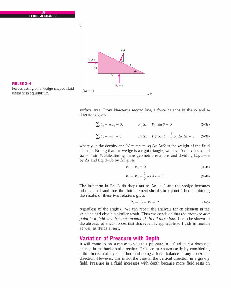
surface area. From Newton’s second law, a force balance in the x- and z-directions gives

(3–3a)

(3–3b)

where r is the density and W " mg " rg $x $z/2 is the weight of the fluidelement. Noting that the wedge is a right triangle, we have $x " l cos u and$z " l sin u. Substituting these geometric relations and dividing Eq. 3–3aby $z and Eq. 3–3b by $x gives

(3–4a)

(3–4b)

The last term in Eq. 3–4b drops out as $z ! 0 and the wedge becomesinfinitesimal, and thus the fluid element shrinks to a point. Then combiningthe results of these two relations gives

(3–5)

regardless of the angle u. We can repeat the analysis for an element in thexz-plane and obtain a similar result. Thus we conclude that the pressure at apoint in a fluid has the same magnitude in all directions. It can be shown inthe absence of shear forces that this result is applicable to fluids in motionas well as fluids at rest.

Variation of Pressure with DepthIt will come as no surprise to you that pressure in a fluid at rest does notchange in the horizontal direction. This can be shown easily by consideringa thin horizontal layer of fluid and doing a force balance in any horizontaldirection. However, this is not the case in the vertical direction in a gravityfield. Pressure in a fluid increases with depth because more fluid rests on

P1 " P2 " P3 " P

P2 # P3 #12

rg $z " 0

P1 # P3 " 0

a Fz " maz " 0: P2 $x # P3l cos u#12 rg $x $z " 0

a Fx " max " 0: P1 $z # P3l sin u" 0

68FLUID MECHANICS

P2 $x

P3l

P1 $z

$x

($y = 1)

z$

z

x

lu

u

FIGURE 3–4Forces acting on a wedge-shaped fluidelement in equilibrium.

cen72367_ch03.qxd 10/29/04 2:21 PM Page 68

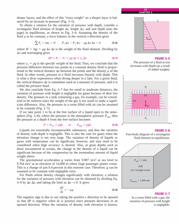
deeper layers, and the effect of this “extra weight” on a deeper layer is bal-anced by an increase in pressure (Fig. 3–5).

To obtain a relation for the variation of pressure with depth, consider arectangular fluid element of height $z, length $x, and unit depth (into thepage) in equilibrium, as shown in Fig. 3–6. Assuming the density of thefluid r to be constant, a force balance in the vertical z-direction gives

(3–6)

where W " mg " rg $x $z is the weight of the fluid element. Dividing by$x and rearranging gives

(3–7)

where gs " rg is the specific weight of the fluid. Thus, we conclude that thepressure difference between two points in a constant density fluid is propor-tional to the vertical distance $z between the points and the density r of thefluid. In other words, pressure in a fluid increases linearly with depth. Thisis what a diver experiences when diving deeper in a lake. For a given fluid,the vertical distance $z is sometimes used as a measure of pressure, and it iscalled the pressure head.

We also conclude from Eq. 3–7 that for small to moderate distances, thevariation of pressure with height is negligible for gases because of their lowdensity. The pressure in a tank containing a gas, for example, can be consid-ered to be uniform since the weight of the gas is too small to make a signif-icant difference. Also, the pressure in a room filled with air can be assumedto be constant (Fig. 3–7).

If we take point 1 to be at the free surface of a liquid open to the atmo-sphere (Fig. 3–8), where the pressure is the atmospheric pressure Patm, thenthe pressure at a depth h from the free surface becomes

(3–8)

Liquids are essentially incompressible substances, and thus the variationof density with depth is negligible. This is also the case for gases when theelevation change is not very large. The variation of density of liquids orgases with temperature can be significant, however, and may need to beconsidered when high accuracy is desired. Also, at great depths such asthose encountered in oceans, the change in the density of a liquid can besignificant because of the compression by the tremendous amount of liquidweight above.

The gravitational acceleration g varies from 9.807 m/s2 at sea level to9.764 m/s2 at an elevation of 14,000 m where large passenger planes cruise.This is a change of just 0.4 percent in this extreme case. Therefore, g can beassumed to be constant with negligible error.

For fluids whose density changes significantly with elevation, a relationfor the variation of pressure with elevation can be obtained by dividing Eq.3–6 by $x $z, and taking the limit as $z ! 0. It gives

(3–9)

The negative sign is due to our taking the positive z direction to be upwardso that dP is negative when dz is positive since pressure decreases in anupward direction. When the variation of density with elevation is known,

dPdz

" #rg

P " Patm ! rgh or Pgage " rgh

$P " P2 # P1 " rg $z " gs $z

a Fz " maz " 0: P2 $x # P1 $x # rg $x $z " 0

69CHAPTER 3

Pgage

FIGURE 3–5The pressure of a fluid at rest

increases with depth (as a result of added weight).

P2

W

P1

x

0

z

z

x

$

$

FIGURE 3–6Free-body diagram of a rectangular

fluid element in equilibrium.

Ptop = 1 atm

AIR

(A 5-m-high room)

Pbottom = 1.006 atm

FIGURE 3–7In a room filled with a gas, the

variation of pressure with height is negligible.

cen72367_ch03.qxd 10/29/04 2:21 PM Page 69

the pressure difference between points 1 and 2 can be determined by inte-gration to be

(3–10)

For constant density and constant gravitational acceleration, this relationreduces to Eq. 3–7, as expected.

Pressure in a fluid at rest is independent of the shape or cross section ofthe container. It changes with the vertical distance, but remains constant inother directions. Therefore, the pressure is the same at all points on a hori-zontal plane in a given fluid. The Dutch mathematician Simon Stevin(1548–1620) published in 1586 the principle illustrated in Fig. 3–9. Notethat the pressures at points A, B, C, D, E, F, and G are the same since theyare at the same depth, and they are interconnected by the same static fluid.However, the pressures at points H and I are not the same since these twopoints cannot be interconnected by the same fluid (i.e., we cannot draw acurve from point I to point H while remaining in the same fluid at alltimes), although they are at the same depth. (Can you tell at which point thepressure is higher?) Also, the pressure force exerted by the fluid is alwaysnormal to the surface at the specified points.

A consequence of the pressure in a fluid remaining constant in the hori-zontal direction is that the pressure applied to a confined fluid increases thepressure throughout by the same amount. This is called Pascal’s law, afterBlaise Pascal (1623–1662). Pascal also knew that the force applied by afluid is proportional to the surface area. He realized that two hydrauliccylinders of different areas could be connected, and the larger could be usedto exert a proportionally greater force than that applied to the smaller. “Pas-cal’s machine” has been the source of many inventions that are a part of ourdaily lives such as hydraulic brakes and lifts. This is what enables us to lift

$P " P2 # P1 " #!2

1

rg dz

70FLUID MECHANICS

P1 = Patm

P2 = Patm + rgh

h

1

2

FIGURE 3–8Pressure in a liquid at rest increaseslinearly with distance from the freesurface.

h

A B C D E

Water

Mercury

F G

IH

Patm

PA = PB = PC = PD = PE = PF = PG = Patm + rgh

PH " PI

FIGURE 3–9The pressure is the same at all points on a horizontal plane in a given fluid regardless of geometry, provided that thepoints are interconnected by the same fluid.

cen72367_ch03.qxd 10/29/04 2:21 PM Page 70

a car easily by one arm, as shown in Fig. 3–10. Noting that P1 " P2 sinceboth pistons are at the same level (the effect of small height differences isnegligible, especially at high pressures), the ratio of output force to inputforce is determined to be

(3–11)

The area ratio A2 /A1 is called the ideal mechanical advantage of the hydrauliclift. Using a hydraulic car jack with a piston area ratio of A2 /A1 " 10, forexample, a person can lift a 1000-kg car by applying a force of just 100 kgf(" 908 N).

3–2 ! THE MANOMETERWe notice from Eq. 3–7 that an elevation change of $z in a fluid at rest cor-responds to $P/rg, which suggests that a fluid column can be used to mea-sure pressure differences. A device based on this principle is called amanometer, and it is commonly used to measure small and moderate pres-sure differences. A manometer mainly consists of a glass or plastic U-tubecontaining one or more fluids such as mercury, water, alcohol, or oil. Tokeep the size of the manometer to a manageable level, heavy fluids such asmercury are used if large pressure differences are anticipated.

Consider the manometer shown in Fig. 3–11 that is used to measure thepressure in the tank. Since the gravitational effects of gases are negligible,the pressure anywhere in the tank and at position 1 has the same value. Fur-thermore, since pressure in a fluid does not vary in the horizontal directionwithin a fluid, the pressure at point 2 is the same as the pressure at point 1,P2 " P1.

The differential fluid column of height h is in static equilibrium, and it isopen to the atmosphere. Then the pressure at point 2 is determined directlyfrom Eq. 3–8 to be

(3–12)

where r is the density of the fluid in the tube. Note that the cross-sectionalarea of the tube has no effect on the differential height h, and thus the pres-sure exerted by the fluid. However, the diameter of the tube should be largeenough (more than a few millimeters) to ensure that the surface tensioneffect and thus the capillary rise is negligible.

EXAMPLE 3–2 Measuring Pressure with a Manometer

A manometer is used to measure the pressure in a tank. The fluid used hasa specific gravity of 0.85, and the manometer column height is 55 cm, asshown in Fig. 3–12. If the local atmospheric pressure is 96 kPa, determinethe absolute pressure within the tank.

SOLUTION The reading of a manometer attached to a tank and theatmospheric pressure are given. The absolute pressure in the tank is to bedetermined.Assumptions The fluid in the tank is a gas whose density is much lowerthan the density of manometer fluid.

P2 " Patm ! rgh

P1 " P2 ! F1

A1 "

F2

A2 ! F2

F1"

A2

A1

71CHAPTER 3

F1 = P1A1

1 2A1P1

F2 = P2 A2

A2P2

FIGURE 3–10Lifting of a large weight by

a small force by the application of Pascal’s law.

Gash

1 2

FIGURE 3–11The basic manometer.

P

SG

= ?h = 55 cm

= 0.85

Patm = 96 kPa

FIGURE 3–12Schematic for Example 3–2.

cen72367_ch03.qxd 10/29/04 2:21 PM Page 71

Properties The specific gravity of the manometer fluid is given to be 0.85.We take the standard density of water to be 1000 kg/m3.Analysis The density of the fluid is obtained by multiplying its specificgravity by the density of water, which is taken to be 1000 kg/m3:

Then from Eq. 3–12,

Discussion Note that the gage pressure in the tank is 4.6 kPa.

Many engineering problems and some manometers involve multipleimmiscible fluids of different densities stacked on top of each other. Suchsystems can be analyzed easily by remembering that (1) the pressure changeacross a fluid column of height h is $P " rgh, (2) pressure increases down-ward in a given fluid and decreases upward (i.e., Pbottom % Ptop), and (3) twopoints at the same elevation in a continuous fluid at rest are at the samepressure.

The last principle, which is a result of Pascal’s law, allows us to “jump”from one fluid column to the next in manometers without worrying aboutpressure change as long as we don’t jump over a different fluid, and thefluid is at rest. Then the pressure at any point can be determined by startingwith a point of known pressure and adding or subtracting rgh terms as weadvance toward the point of interest. For example, the pressure at the bot-tom of the tank in Fig. 3–13 can be determined by starting at the free sur-face where the pressure is Patm, moving downward until we reach point 1 atthe bottom, and setting the result equal to P1. It gives

In the special case of all fluids having the same density, this relation reducesto Eq. 3–12, as expected.

Manometers are particularly well-suited to measure pressure drops acrossa horizontal flow section between two specified points due to the presenceof a device such as a valve or heat exchanger or any resistance to flow. Thisis done by connecting the two legs of the manometer to these two points, asshown in Fig. 3–14. The working fluid can be either a gas or a liquid whosedensity is r1. The density of the manometer fluid is r2, and the differentialfluid height is h.

A relation for the pressure difference P1 # P2 can be obtained by startingat point 1 with P1, moving along the tube by adding or subtracting the rghterms until we reach point 2, and setting the result equal to P2:

(3–13)

Note that we jumped from point A horizontally to point B and ignored thepart underneath since the pressure at both points is the same. Simplifying,

(3–14)P1 # P2 " (r2 # r1)gh

P1 ! r1g(a ! h) # r2gh # r1ga " P2

Patm ! r1gh1 ! r2gh2 ! r3gh3 " P1

" 100.6 kPa

" 96 kPa ! (850 kg&m3)(9.81 m&s2)(0.55 m)a 1 N1 kg ' m&s2b a 1 kPa

1000 N&m2bP " Patm ! rgh

r " SG (rH2O) " (0.85)(1000 kg&m3) " 850 kg&m3

72FLUID MECHANICS

Patm

1h3

h2

h1

Fluid 2

Fluid 1

Fluid 3

FIGURE 3–13In stacked-up fluid layers, the pressurechange across a fluid layer of densityr and height h is rgh.

a

hr1

A B

Fluid

A flow sectionor flow device

1 2

r2

FIGURE 3–14Measuring the pressure drop across aflow section or a flow device by adifferential manometer.

cen72367_ch03.qxd 10/29/04 2:21 PM Page 72

Note that the distance a has no effect on the result, but must be included inthe analysis. Also, when the fluid flowing in the pipe is a gas, then r1 ! r2and the relation in Eq. 3–14 simplifies to P1 ! P2 r2gh.

EXAMPLE 3–3 Measuring Pressure with a Multifluid Manometer

The water in a tank is pressurized by air, and the pressure is measured by amultifluid manometer as shown in Fig. 3–15. The tank is located on a moun-tain at an altitude of 1400 m where the atmospheric pressure is 85.6 kPa.Determine the air pressure in the tank if h1 " 0.1 m, h2 " 0.2 m, and h3 "0.35 m. Take the densities of water, oil, and mercury to be 1000 kg/m3,850 kg/m3, and 13,600 kg/m3, respectively.

SOLUTION The pressure in a pressurized water tank is measured by a multi-fluid manometer. The air pressure in the tank is to be determined.Assumption The air pressure in the tank is uniform (i.e., its variation withelevation is negligible due to its low density), and thus we can determine thepressure at the air–water interface.Properties The densities of water, oil, and mercury are given to be1000 kg/m3, 850 kg/m3, and 13,600 kg/m3, respectively.Analysis Starting with the pressure at point 1 at the air–water interface,moving along the tube by adding or subtracting the rgh terms until we reachpoint 2, and setting the result equal to Patm since the tube is open to theatmosphere gives

Solving for P1 and substituting,

Discussion Note that jumping horizontally from one tube to the next andrealizing that pressure remains the same in the same fluid simplifies theanalysis considerably. Also note that mercury is a toxic fluid, and mercurymanometers and thermometers are being replaced by ones with safer fluidsbecause of the risk of exposure to mercury vapor during an accident.

EXAMPLE 3–4 Analyzing a Multifluid Manometer with EES

Reconsider the multifluid manometer discussed in Example 3–3. Determinethe air pressure in the tank using EES. Also determine what the differentialfluid height h3 would be for the same air pressure if the mercury in the lastcolumn were replaced by seawater with a density of 1030 kg/m3.

SOLUTION The pressure in a water tank is measured by a multifluidmanometer. The air pressure in the tank and the differential fluid height h3if mercury is replaced by seawater are to be determined using EES.

" 130 kPa

! (850 kg#m3)(0.2 m)]a 1 N1 kg $ m#s2b a 1 kPa

1000 N#m2b

" 85.6 kPa % (9.81 m#s2)[(13,600 kg#m3)(0.35 m) ! (1000 kg#m3)(0.1 m)

" Patm % g(rmercuryh3 ! rwaterh1 ! roilh2)

P1 " Patm ! rwatergh1 ! roilgh2 % rmercurygh3

P1 % rwatergh1 % roilgh2 ! rmercurygh3 " Patm

73CHAPTER 3

h1

h2h3

Oil

Mercury

WATER

AIR

1

2

FIGURE 3–15Schematic for Example 3–3; drawing

not to scale.

cen72367_ch03.qxd 11/19/04 10:33 AM Page 73

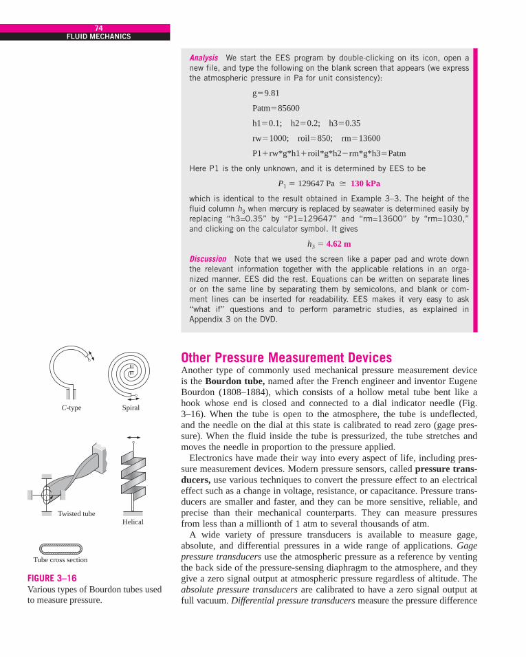
Analysis We start the EES program by double-clicking on its icon, open anew file, and type the following on the blank screen that appears (we expressthe atmospheric pressure in Pa for unit consistency):

Here P1 is the only unknown, and it is determined by EES to be

which is identical to the result obtained in Example 3–3. The height of thefluid column h3 when mercury is replaced by seawater is determined easily byreplacing “h3=0.35” by “P1=129647” and “rm=13600” by “rm=1030,”and clicking on the calculator symbol. It gives

Discussion Note that we used the screen like a paper pad and wrote downthe relevant information together with the applicable relations in an orga-nized manner. EES did the rest. Equations can be written on separate linesor on the same line by separating them by semicolons, and blank or com-ment lines can be inserted for readability. EES makes it very easy to ask“what if” questions and to perform parametric studies, as explained inAppendix 3 on the DVD.

Other Pressure Measurement DevicesAnother type of commonly used mechanical pressure measurement deviceis the Bourdon tube, named after the French engineer and inventor EugeneBourdon (1808–1884), which consists of a hollow metal tube bent like ahook whose end is closed and connected to a dial indicator needle (Fig.3–16). When the tube is open to the atmosphere, the tube is undeflected,and the needle on the dial at this state is calibrated to read zero (gage pres-sure). When the fluid inside the tube is pressurized, the tube stretches andmoves the needle in proportion to the pressure applied.

Electronics have made their way into every aspect of life, including pres-sure measurement devices. Modern pressure sensors, called pressure trans-ducers, use various techniques to convert the pressure effect to an electricaleffect such as a change in voltage, resistance, or capacitance. Pressure trans-ducers are smaller and faster, and they can be more sensitive, reliable, andprecise than their mechanical counterparts. They can measure pressuresfrom less than a millionth of 1 atm to several thousands of atm.

A wide variety of pressure transducers is available to measure gage,absolute, and differential pressures in a wide range of applications. Gagepressure transducers use the atmospheric pressure as a reference by ventingthe back side of the pressure-sensing diaphragm to the atmosphere, and theygive a zero signal output at atmospheric pressure regardless of altitude. Theabsolute pressure transducers are calibrated to have a zero signal output atfull vacuum. Differential pressure transducers measure the pressure difference

h3 " 4.62 m

P1 " 129647 Pa " 130 kPa

P1!rw*g*h1!roil*g*h2#rm*g*h3"Patm

rw"1000; roil"850; rm"13600

h1"0.1; h2"0.2; h3"0.35

Patm"85600

g"9.81

74FLUID MECHANICS

C-type Spiral

Twisted tube

Tube cross section

Helical

FIGURE 3–16Various types of Bourdon tubes usedto measure pressure.

cen72367_ch03.qxd 10/29/04 2:21 PM Page 74

between two locations directly instead of using two pressure transducersand taking their difference.

Strain-gage pressure transducers work by having a diaphragm deflectbetween two chambers open to the pressure inputs. As the diaphragmstretches in response to a change in pressure difference across it, the straingage stretches and a Wheatstone bridge circuit amplifies the output. Acapacitance transducer works similarly, but capacitance change is measuredinstead of resistance change as the diaphragm stretches.

Piezoelectric transducers, also called solid-state pressure transducers,work on the principle that an electric potential is generated in a crystallinesubstance when it is subjected to mechanical pressure. This phenomenon,first discovered by brothers Pierre and Jacques Curie in 1880, is called thepiezoelectric (or press-electric) effect. Piezoelectric pressure transducershave a much faster frequency response compared to the diaphragm units andare very suitable for high-pressure applications, but they are generally not assensitive as the diaphragm-type transducers.

3–3 ! THE BAROMETER AND ATMOSPHERIC PRESSURE

Atmospheric pressure is measured by a device called a barometer; thus, theatmospheric pressure is often referred to as the barometric pressure.

The Italian Evangelista Torricelli (1608–1647) was the first to conclu-sively prove that the atmospheric pressure can be measured by inverting amercury-filled tube into a mercury container that is open to the atmosphere,as shown in Fig. 3–17. The pressure at point B is equal to the atmosphericpressure, and the pressure at C can be taken to be zero since there is onlymercury vapor above point C and the pressure is very low relative to Patmand can be neglected to an excellent approximation. Writing a force balancein the vertical direction gives

(3–15)

where r is the density of mercury, g is the local gravitational acceleration,and h is the height of the mercury column above the free surface. Note thatthe length and the cross-sectional area of the tube have no effect on theheight of the fluid column of a barometer (Fig. 3–18).

A frequently used pressure unit is the standard atmosphere, which isdefined as the pressure produced by a column of mercury 760 mm in heightat 0°C (rHg " 13,595 kg/m3) under standard gravitational acceleration (g " 9.807 m/s2). If water instead of mercury were used to measure thestandard atmospheric pressure, a water column of about 10.3 m would beneeded. Pressure is sometimes expressed (especially by weather forecasters)in terms of the height of the mercury column. The standard atmosphericpressure, for example, is 760 mmHg (29.92 inHg) at 0°C. The unit mmHgis also called the torr in honor of Torricelli. Therefore, 1 atm " 760 torrand 1 torr " 133.3 Pa.

The standard atmospheric pressure Patm changes from 101.325 kPa at sealevel to 89.88, 79.50, 54.05, 26.5, and 5.53 kPa at altitudes of 1000, 2000,5000, 10,000, and 20,000 meters, respectively. The standard atmosphericpressure in Denver (elevation " 1610 m), for example, is 83.4 kPa.

Patm " rgh

75CHAPTER 3

hW rghA=

Ah

B

Mercury

C

Patm

FIGURE 3–17The basic barometer.

A2A1 A3

FIGURE 3–18The length or the cross-sectional areaof the tube has no effect on the height

of the fluid column of a barometer,provided that the tube diameter is

large enough to avoid surface tension(capillary) effects.

cen72367_ch03.qxd 10/29/04 2:21 PM Page 75

76FLUID MECHANICS

Engine Lungs

FIGURE 3–19At high altitudes, a car enginegenerates less power and a person gets less oxygen because of the lower density of air.

Remember that the atmospheric pressure at a location is simply theweight of the air above that location per unit surface area. Therefore, itchanges not only with elevation but also with weather conditions.

The decline of atmospheric pressure with elevation has far-reaching rami-fications in daily life. For example, cooking takes longer at high altitudessince water boils at a lower temperature at lower atmospheric pressures.Nose bleeding is a common experience at high altitudes since the differencebetween the blood pressure and the atmospheric pressure is larger in thiscase, and the delicate walls of veins in the nose are often unable to with-stand this extra stress.

For a given temperature, the density of air is lower at high altitudes, andthus a given volume contains less air and less oxygen. So it is no surprisethat we tire more easily and experience breathing problems at high altitudes.To compensate for this effect, people living at higher altitudes develop moreefficient lungs. Similarly, a 2.0-L car engine will act like a 1.7-L car engineat 1500 m altitude (unless it is turbocharged) because of the 15 percent dropin pressure and thus 15 percent drop in the density of air (Fig. 3–19). A fanor compressor will displace 15 percent less air at that altitude for the samevolume displacement rate. Therefore, larger cooling fans may need to beselected for operation at high altitudes to ensure the specified mass flowrate. The lower pressure and thus lower density also affects lift and drag:airplanes need a longer runway at high altitudes to develop the required lift,and they climb to very high altitudes for cruising for reduced drag and thusbetter fuel efficiency.

EXAMPLE 3–5 Measuring Atmospheric Pressure with aBarometer

Determine the atmospheric pressure at a location where the barometric read-ing is 740 mm Hg and the gravitational acceleration is g " 9.81 m/s2.Assume the temperature of mercury to be 10°C, at which its density is13,570 kg/m3.

SOLUTION The barometric reading at a location in height of mercury col-umn is given. The atmospheric pressure is to be determined.Assumptions The temperature of mercury is assumed to be 10°C.Properties The density of mercury is given to be 13,570 kg/m3.Analysis From Eq. 3–15, the atmospheric pressure is determined to be

Discussion Note that density changes with temperature, and thus this effectshould be considered in calculations.

EXAMPLE 3–6 Effect of Piston Weight on Pressure in a Cylinder

The piston of a vertical piston–cylinder device containing a gas has a massof 60 kg and a cross-sectional area of 0.04 m2, as shown in Fig. 3–20. The

" 98.5 kPa

" (13,570 kg&m3)(9.81 m&s2)(0.74 m)a 1 N1 kg ' m&s2b a 1 kPa

1000 N&m2bPatm " rgh

cen72367_ch03.qxd 10/29/04 2:21 PM Page 76

77CHAPTER 3

A = 0.04 m2

P = ?

Patm = 0.97 barm = 60 kg

Patm

W = mg

P

FIGURE 3–20Schematic for Example 3–6, and the

free-body diagram of the piston.

Increasing salinityand density

Surface zone

Sun

r0 = 1040 kg/m3

H = 4 m

zGradient zone

Storage zone

1

2 FIGURE 3–21Schematic for Example 3–7.

local atmospheric pressure is 0.97 bar, and the gravitational acceleration is9.81 m/s2. (a) Determine the pressure inside the cylinder. (b) If some heat istransferred to the gas and its volume is doubled, do you expect the pressureinside the cylinder to change?

SOLUTION A gas is contained in a vertical cylinder with a heavy piston. Thepressure inside the cylinder and the effect of volume change on pressure areto be determined.Assumptions Friction between the piston and the cylinder is negligible.Analysis (a) The gas pressure in the piston–cylinder device depends on theatmospheric pressure and the weight of the piston. Drawing the free-bodydiagram of the piston as shown in Fig. 3–20 and balancing the verticalforces yield

Solving for P and substituting,

(b) The volume change will have no effect on the free-body diagram drawn inpart (a), and therefore the pressure inside the cylinder will remain the same.Discussion If the gas behaves as an ideal gas, the absolute temperaturedoubles when the volume is doubled at constant pressure.

EXAMPLE 3–7 Hydrostatic Pressure in a Solar Pond with Variable Density

Solar ponds are small artificial lakes of a few meters deep that are used tostore solar energy. The rise of heated (and thus less dense) water to the sur-face is prevented by adding salt at the pond bottom. In a typical salt gradi-ent solar pond, the density of water increases in the gradient zone, as shownin Fig. 3–21, and the density can be expressed as

where r0 is the density on the water surface, z is the vertical distance mea-sured downward from the top of the gradient zone, and H is the thickness of

r " r0B1 ! tan2ap4

zHb

" 1.12 bars

" 0.97 bar !(60 kg)(9.81 m&s2)

0.04 m2 a 1 N1 kg ' m&s2b a 1 bar

105 N&m2bP " Patm !

mg

A

PA " Patm A ! W

cen72367_ch03.qxd 10/29/04 2:21 PM Page 77

the gradient zone. For H " 4 m, r0 " 1040 kg/m3, and a thickness of 0.8m for the surface zone, calculate the gage pressure at the bottom of the gra-dient zone.

SOLUTION The variation of density of saline water in the gradient zone of asolar pond with depth is given. The gage pressure at the bottom of the gradi-ent zone is to be determined.Assumptions The density in the surface zone of the pond is constant.Properties The density of brine on the surface is given to be 1040 kg/m3.Analysis We label the top and the bottom of the gradient zone as 1 and 2,respectively. Noting that the density of the surface zone is constant, the gagepressure at the bottom of the surface zone (which is the top of the gradientzone) is

since 1 kN/m2 " 1 kPa. The differential change in hydrostatic pressureacross a vertical distance of dz is given by

Integrating from the top of the gradient zone (point 1 where z " 0) to anylocation z in the gradient zone (no subscript) gives

Performing the integration gives the variation of gage pressure in the gradi-ent zone to be

Then the pressure at the bottom of the gradient zone (z " H " 4 m)becomes

Discussion The variation of gage pressure in the gradient zone with depth isplotted in Fig. 3–22. The dashed line indicates the hydrostatic pressure forthe case of constant density at 1040 kg/m3 and is given for reference. Notethat the variation of pressure with depth is not linear when density varieswith depth.

3–4 ! INTRODUCTION TO FLUID STATICSFluid statics deals with problems associated with fluids at rest. The fluidcan be either gaseous or liquid. Fluid statics is generally referred to ashydrostatics when the fluid is a liquid and as aerostatics when the fluid is agas. In fluid statics, there is no relative motion between adjacent fluid lay-ers, and thus there are no shear (tangential) stresses in the fluid trying todeform it. The only stress we deal with in fluid statics is the normal stress,which is the pressure, and the variation of pressure is due only to the weightof the fluid. Therefore, the topic of fluid statics has significance only in

" 54.0 kPa (gage)

P2 " 8.16 kPa ! (1040 kg&m3)(9.81 m&s2) 4(4 m)p

sinh#1atan p

4 44b a 1 kN

1000 kg ' m&s2bP " P1 ! r0g

4Hp

sinh#1atan p

4

zHb

P # P1 " !z

0

rg dz ! P " P1 ! !z

0

r0B1 ! tan2ap4

zHbg dz

dP " rg dz

P1 " rgh1 " (1040 kg&m3)(9.81 m&s2)(0.8 m)a 1 kN1000 kg ' m&s2b " 8.16 kPa

78FLUID MECHANICS

4

3

2

3.5

2.5

1.5

1

0.5

0

0 10 20 30P, kPa

z, m

40 50 60

FIGURE 3–22The variation of gage pressure withdepth in the gradient zone of the solar pond.

cen72367_ch03.qxd 10/29/04 2:21 PM Page 78

gravity fields, and the force relations developed naturally involve the gravi-tational acceleration g. The force exerted on a surface by a fluid at rest isnormal to the surface at the point of contact since there is no relative motionbetween the fluid and the solid surface, and thus no shear forces can act par-allel to the surface.

Fluid statics is used to determine the forces acting on floating or sub-merged bodies and the forces developed by devices like hydraulic pressesand car jacks. The design of many engineering systems such as water damsand liquid storage tanks requires the determination of the forces acting onthe surfaces using fluid statics. The complete description of the resultanthydrostatic force acting on a submerged surface requires the determinationof the magnitude, the direction, and the line of action of the force. In Sec-tions 3–5 and 3–6, we consider the forces acting on both plane and curvedsurfaces of submerged bodies due to pressure.

3–5 ! HYDROSTATIC FORCES ON SUBMERGED PLANE SURFACES

A plate exposed to a liquid, such as a gate valve in a dam, the wall of a liq-uid storage tank, or the hull of a ship at rest, is subjected to fluid pressuredistributed over its surface (Fig. 3–23). On a plane surface, the hydrostaticforces form a system of parallel forces, and we often need to determine themagnitude of the force and its point of application, which is called the cen-ter of pressure. In most cases, the other side of the plate is open to theatmosphere (such as the dry side of a gate), and thus atmospheric pressureacts on both sides of the plate, yielding a zero resultant. In such cases, it isconvenient to subtract atmospheric pressure and work with the gage pres-sure only (Fig. 3–24). For example, Pgage " rgh at the bottom of the lake.

Consider the top surface of a flat plate of arbitrary shape completely sub-merged in a liquid, as shown in Fig. 3–25 together with its top view. Theplane of this surface (normal to the page) intersects the horizontal free sur-face with an angle u, and we take the line of intersection to be the x-axis.The absolute pressure above the liquid is P0, which is the local atmosphericpressure Patm if the liquid is open to the atmosphere (but P0 may be different

79CHAPTER 3

FIGURE 3–23Hoover Dam.

Courtesy United States Department of the Interior,Bureau of Reclamation-Lower Colorado Region.

Patm

Patm + rgh

h #

(a) Patm considered (b) Patm subtracted

rgh

FIGURE 3–24When analyzing hydrostatic forces onsubmerged surfaces, the atmospheric

pressure can be subtracted forsimplicity when it acts on both

sides of the structure.

cen72367_ch03.qxd 10/29/04 2:21 PM Page 79

than Patm if the space above the liquid is evacuated or pressurized). Then theabsolute pressure at any point on the plate is

(3–16)

where h is the vertical distance of the point from the free surface and y isthe distance of the point from the x-axis (from point O in Fig. 3–25). Theresultant hydrostatic force FR acting on the surface is determined by inte-grating the force P dA acting on a differential area dA over the entire sur-face area,

(3–17)

But the first moment of area is related to the y-coordinate of the

centroid (or center) of the surface by

(3–18)

Substituting,

(3–19)

where PC " P0 ! rghC is the pressure at the centroid of the surface, whichis equivalent to the average pressure on the surface, and hC " yC sin u is thevertical distance of the centroid from the free surface of the liquid (Fig.3–26). Thus we conclude that:

The magnitude of the resultant force acting on a plane surface of acompletely submerged plate in a homogeneous (constant density) fluid is equal to the product of the pressure PC at the centroid of the surface and the area A of the surface (Fig. 3–27).

The pressure P0 is usually atmospheric pressure, which can be ignored inmost cases since it acts on both sides of the plate. When this is not the case,a practical way of accounting for the contribution of P0 to the resultant

FR " (P0 ! rgyC sin u)A " (P0 ! rghC)A " PC A " Pave A

yC "1A

!A

y dA

!A

y dA

FR " !A

P dA " !A

(P0 ! rgy sin u) dA " P0 A ! rg sin u !A

y dA

P " P0 ! rgh " P0 ! rgy sin u

80FLUID MECHANICS

dA

CCP Centroid

Center of pressurePlane surfaceof area A

h = y sin

P = P0 + rgy sin u OPC = Pave

FR = PC APressure prismof volume V

Pressuredistribution

yy

z

yC

A dA

Plane surfaceP = P0 + rgh

V = !dV = !P dA = FR

uu

FIGURE 3–25Hydrostatic force on an inclined plane surface completely submerged in a liquid.

Free surface

hC

Patm

= PC = Patm + rghCPave

Centroidof surface

FIGURE 3–26The pressure at the centroid of asurface is equivalent to the averagepressure on the surface.

cen72367_ch03.qxd 10/29/04 2:21 PM Page 80

81CHAPTER 3

Center ofpressure Centroid

of area

Line of action

O

PCFR = PC A

yC

yPz

u

FIGURE 3–27The resultant force acting on a planesurface is equal to the product of the

pressure at the centroid of the surfaceand the surface area, and its line ofaction passes through the center of

pressure.

force is simply to add an equivalent depth hequiv " P0 /rg to hC; that is, toassume the presence of an additional liquid layer of thickness hequiv on topof the liquid with absolute vacuum above.

Next we need to determine the line of action of the resultant force FR.Two parallel force systems are equivalent if they have the same magnitudeand the same moment about any point. The line of action of the resultanthydrostatic force, in general, does not pass through the centroid of the sur-face—it lies underneath where the pressure is higher. The point of intersec-tion of the line of action of the resultant force and the surface is the centerof pressure. The vertical location of the line of action is determined byequating the moment of the resultant force to the moment of the distributedpressure force about the x-axis. It gives

or(3–20)

where yP is the distance of the center of pressure from the x-axis (point O in

Fig. 3–27) and is the second moment of area (also called

the area moment of inertia) about the x-axis. The second moments of areaare widely available for common shapes in engineering handbooks, but theyare usually given about the axes passing through the centroid of the area.Fortunately, the second moments of area about two parallel axes are relatedto each other by the parallel axis theorem, which in this case is expressed as

(3–21)

where Ixx, C is the second moment of area about the x-axis passing throughthe centroid of the area and yC (the y-coordinate of the centroid) is the dis-tance between the two parallel axes. Substituting the FR relation from Eq.3–19 and the Ixx, O relation from Eq. 3–21 into Eq. 3–20 and solving for yPgives

(3–22a)

For P0 " 0, which is usually the case when the atmospheric pressure isignored, it simplifies to

(3–22b)

Knowing yP, the vertical distance of the center of pressure from the free sur-face is determined from hP " yP sin u.

The Ixx, C values for some common areas are given in Fig. 3–28. For theseand other areas that possess symmetry about the y-axis, the center of pres-sure lies on the y-axis directly below the centroid. The location of the centerof pressure in such cases is simply the point on the surface of the verticalplane of symmetry at a distance hP from the free surface.

Pressure acts normal to the surface, and the hydrostatic forces acting on aflat plate of any shape form a volume whose base is the plate area and

yP " yC !Ixx, C

yC A

yP " yC !Ixx, C

[yC ! P0 &(rg sin u)]A

Ixx, O " Ixx, C ! y 2C A

Ixx, O " !A

y2 dA

yPFR "P0 yC A ! rg sin u Ixx, O

yPFR " !A

yP dA " !A

y(P0 ! rgy sin u) dA " P0 !A

y dA ! rg sin u !A

y2 dA

cen72367_ch03.qxd 10/29/04 2:21 PM Page 81

82FLUID MECHANICS

b/2

bC C C

b/2

A = ab, Ixx, C = ab3/12

a/2a/2

y

x

(a) Rectangle

R

R

R

A = pR2, Ixx, C = pR4/4

b

a

y

x

(b) Circle

A = pab, Ixx, C = pab3/4

y

x

(c) Ellipse

2b/3

b/3

C C C

A = ab/2, Ixx, C = ab3/36

a/2a/2

y

x

(d) Triangle

R

A = pR2/2, Ixx, C = 0.109757R4

a

y

x

(e) Semicircle

A = pab/2, Ixx, C = 0.109757ab3

y

x

( f ) Semiellipse

b

4b3p

4R3p

FIGURE 3–28The centroid and the centroidal moments of inertia for some common geometries.

whose height is the linearly varying pressure, as shown in Fig. 3–29. Thisvirtual pressure prism has an interesting physical interpretation: its volumeis equal to the magnitude of the resultant hydrostatic force acting on theplate since V " # P dA, and the line of action of this force passes throughthe centroid of this homogeneous prism. The projection of the centroid onthe plate is the pressure center. Therefore, with the concept of pressureprism, the problem of describing the resultant hydrostatic force on a planesurface reduces to finding the volume and the two coordinates of the cen-troid of this pressure prism.

Special Case: Submerged Rectangular PlateConsider a completely submerged rectangular flat plate of height b andwidth a tilted at an angle u from the horizontal and whose top edge is hori-zontal and is at a distance s from the free surface along the plane of theplate, as shown in Fig. 3–30a. The resultant hydrostatic force on the uppersurface is equal to the average pressure, which is the pressure at the mid-point of the surface, times the surface area A. That is,

Tilted rectangular plate: (3–23)FR " PC A " [P0 ! rg(s ! b/2) sin u]ab

cen72367_ch03.qxd 10/29/04 2:21 PM Page 82

The force acts at a vertical distance of hP " yP sin u from the free surfacedirectly beneath the centroid of the plate where, from Eq. 3–22a,

(3–24)

When the upper edge of the plate is at the free surface and thus s " 0, Eq.3–23 reduces to

Tilted rectangular plate (s " 0): (3–25)FR " [P0 ! rg(b sin u)&2]ab

" s !b2

!b2

12[s ! b&2 ! P0 &(rg sin u)]

yP " s !b2

!ab3&12

[s ! b&2 ! P0 &(rg sin u)]ab

83CHAPTER 3

Surfacea

b

P

Pressureprism

FIGURE 3–29The hydrostatic forces acting on a

plane surface form a volume whosebase (left face) is the surface and

whose height is the pressure.

O

$

syp

b

O

s

yp

b

FR = [P0 + rg(s + b/2) sin u]ab FR = [P0 + rg(s + b/2)]ab

FR = (P0 + rgh)ab

(b) Vertical plate (c) Horizontal plate(a) Tilted plate

a

h

P0 P0 P0

FIGURE 3–30Hydrostatic force acting on the top surface of a submerged rectangular plate for tilted, vertical, and horizontal cases.

cen72367_ch03.qxd 10/29/04 2:21 PM Page 83

For a completely submerged vertical plate (u " 90°) whose top edge is hori-zontal, the hydrostatic force can be obtained by setting sin u " 1 (Fig. 3–30b)

Vertical rectangular plate: (3–26)

Vertical rectangular plate (s " 0): (3–27)

When the effect of P0 is ignored since it acts on both sides of the plate, thehydrostatic force on a vertical rectangular surface of height b whose topedge is horizontal and at the free surface is FR " rgab2/2 acting at a dis-tance of 2b/3 from the free surface directly beneath the centroid of the plate.

The pressure distribution on a submerged horizontal surface is uniform,and its magnitude is P " P0 ! rgh, where h is the distance of the surfacefrom the free surface. Therefore, the hydrostatic force acting on a horizontalrectangular surface is

Horizontal rectangular plate: (3–28)

and it acts through the midpoint of the plate (Fig. 3–30c).

EXAMPLE 3–8 Hydrostatic Force Acting on the Door of a Submerged Car

A heavy car plunges into a lake during an accident and lands at the bottomof the lake on its wheels (Fig. 3–31). The door is 1.2 m high and 1 m wide,and the top edge of the door is 8 m below the free surface of the water.Determine the hydrostatic force on the door and the location of the pressurecenter, and discuss if the driver can open the door.

SOLUTION A car is submerged in water. The hydrostatic force on the dooris to be determined, and the likelihood of the driver opening the door is tobe assessed.Assumptions 1 The bottom surface of the lake is horizontal. 2 The passen-ger cabin is well-sealed so that no water leaks inside. 3 The door can beapproximated as a vertical rectangular plate. 4 The pressure in the passengercabin remains at atmospheric value since there is no water leaking in, and

FR " (P0 ! rgh)ab

FR " (P0 ! rgb& 2)ab

FR " [P0 ! rg(s ! b& 2)]ab

84FLUID MECHANICS

1.2 m

8 m

Lake

1 m

FIGURE 3–31Schematic for Example 3–8.

cen72367_ch03.qxd 10/29/04 2:21 PM Page 84

85CHAPTER 3

thus no compression of the air inside. Therefore, atmospheric pressure can-cels out in the calculations since it acts on both sides of the door. 5 Theweight of the car is larger than the buoyant force acting on it.Properties We take the density of lake water to be 1000 kg/m3 throughout.Analysis The average pressure on the door is the pressure value at the cen-troid (midpoint) of the door and is determined to be

Then the resultant hydrostatic force on the door becomes

The pressure center is directly under the midpoint of the door, and its dis-tance from the surface of the lake is determined from Eq. 3–24 by settingP0 " 0 to be

Discussion A strong person can lift 100 kg, whose weight is 981 N or about1 kN. Also, the person can apply the force at a point farthest from thehinges (1 m farther) for maximum effect and generate a moment of 1 kN · m.The resultant hydrostatic force acts under the midpoint of the door, and thus adistance of 0.5 m from the hinges. This generates a moment of 50.6 kN · m,which is about 50 times the moment the driver can possibly generate. There-fore, it is impossible for the driver to open the door of the car. The driver’sbest bet is to let some water in (by rolling the window down a little, forexample) and to keep his or her head close to the ceiling. The driver shouldbe able to open the door shortly before the car is filled with water since atthat point the pressures on both sides of the door are nearly the same andopening the door in water is almost as easy as opening it in air.

3–6 ! HYDROSTATIC FORCES ON SUBMERGED CURVED SURFACES

For a submerged curved surface, the determination of the resultant hydrosta-tic force is more involved since it typically requires the integration of thepressure forces that change direction along the curved surface. The conceptof the pressure prism in this case is not much help either because of thecomplicated shapes involved.

The easiest way to determine the resultant hydrostatic force FR acting ona two-dimensional curved surface is to determine the horizontal and verticalcomponents FH and FV separately. This is done by considering the free-bodydiagram of the liquid block enclosed by the curved surface and the twoplane surfaces (one horizontal and one vertical) passing through the twoends of the curved surface, as shown in Fig. 3–32. Note that the vertical sur-face of the liquid block considered is simply the projection of the curvedsurface on a vertical plane, and the horizontal surface is the projection ofthe curved surface on a horizontal plane. The resultant force acting on the

yP " s !b2

!b2

12(s ! b&2)" 8 !

1.22

!1.22

12(8 ! 1.2&2)" 8.61 m

FR " Pave A " (84.4 kN&m2) (1 m ( 1.2 m) " 101.3 kN

" 84.4 kN&m2

" (1000 kg&m3)(9.81 m&s2)(8 ! 1.2&2 m)a 1 kN1000 kg ' m&s2b

Pave " PC " rghC " rg(s ! b&2)

cen72367_ch03.qxd 10/29/04 2:21 PM Page 85

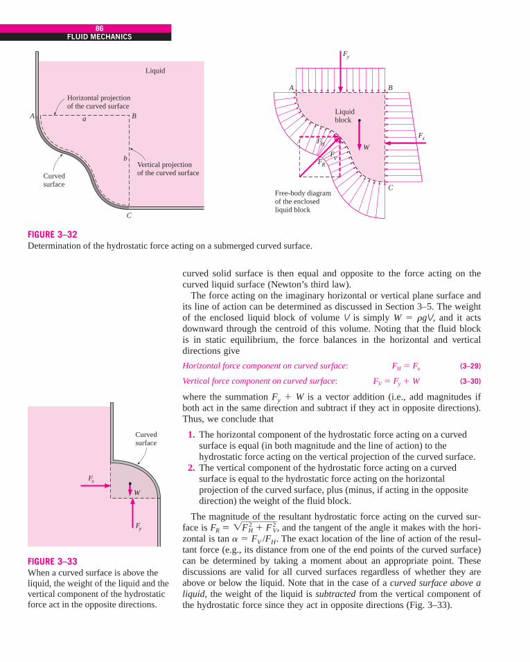
curved solid surface is then equal and opposite to the force acting on thecurved liquid surface (Newton’s third law).

The force acting on the imaginary horizontal or vertical plane surface andits line of action can be determined as discussed in Section 3–5. The weightof the enclosed liquid block of volume V is simply W " rgV, and it actsdownward through the centroid of this volume. Noting that the fluid blockis in static equilibrium, the force balances in the horizontal and verticaldirections give

Horizontal force component on curved surface: (3–29)

Vertical force component on curved surface: (3–30)

where the summation Fy ! W is a vector addition (i.e., add magnitudes ifboth act in the same direction and subtract if they act in opposite directions).Thus, we conclude that

1. The horizontal component of the hydrostatic force acting on a curvedsurface is equal (in both magnitude and the line of action) to thehydrostatic force acting on the vertical projection of the curved surface.

2. The vertical component of the hydrostatic force acting on a curvedsurface is equal to the hydrostatic force acting on the horizontalprojection of the curved surface, plus (minus, if acting in the oppositedirection) the weight of the fluid block.

The magnitude of the resultant hydrostatic force acting on the curved sur-face is , and the tangent of the angle it makes with the hori-zontal is tan a " FV /FH. The exact location of the line of action of the resul-tant force (e.g., its distance from one of the end points of the curved surface)can be determined by taking a moment about an appropriate point. Thesediscussions are valid for all curved surfaces regardless of whether they areabove or below the liquid. Note that in the case of a curved surface above aliquid, the weight of the liquid is subtracted from the vertical component ofthe hydrostatic force since they act in opposite directions (Fig. 3–33).

FR " 1F 2H ! F 2

V

FV " Fy ! W

FH " Fx

86FLUID MECHANICS

Horizontal projectionof the curved surface

Curvedsurface

Liquid

Liquidblock

Vertical projectionof the curved surface

Free-body diagramof the enclosedliquid block

aA B

A B

C

C

b

FH

FR

Fx

Fy

WF

V

FIGURE 3–32Determination of the hydrostatic force acting on a submerged curved surface.

Curvedsurface

W

Fx

Fy

FIGURE 3–33When a curved surface is above theliquid, the weight of the liquid and thevertical component of the hydrostaticforce act in the opposite directions.

cen72367_ch03.qxd 10/29/04 2:21 PM Page 86

87CHAPTER 3

O

FR

Resultantforce

Circularsurface

Pressureforces

FIGURE 3–34The hydrostatic force acting on a

circular surface always passes through the center of the circle sincethe pressure forces are normal to the

surface and they all pass through the center.

FR1b1

FR2b2

Oil

Water

FIGURE 3–35The hydrostatic force on a surface

submerged in a multilayered fluid canbe determined by considering parts of

the surface in different fluids asdifferent surfaces.

When the curved surface is a circular arc (full circle or any part of it), theresultant hydrostatic force acting on the surface always passes throughthe center of the circle. This is because the pressure forces are normal to thesurface, and all lines normal to the surface of a circle pass through the cen-ter of the circle. Thus, the pressure forces form a concurrent force system atthe center, which can be reduced to a single equivalent force at that point(Fig. 3–34).

Finally, hydrostatic forces acting on a plane or curved surface submergedin a multilayered fluid of different densities can be determined by consid-ering different parts of surfaces in different fluids as different surfaces, find-ing the force on each part, and then adding them using vector addition. Fora plane surface, it can be expressed as (Fig. 3–35)

Plane surface in a multilayered fluid: (3–31)

where PC, i " P0 ! righC, i is the pressure at the centroid of the portion ofthe surface in fluid i and Ai is the area of the plate in that fluid. The line ofaction of this equivalent force can be determined from the requirement thatthe moment of the equivalent force about any point is equal to the sum ofthe moments of the individual forces about the same point.

EXAMPLE 3–9 A Gravity-Controlled Cylindrical Gate

A long solid cylinder of radius 0.8 m hinged at point A is used as an auto-matic gate, as shown in Fig. 3–36. When the water level reaches 5 m, thegate opens by turning about the hinge at point A. Determine (a) the hydro-static force acting on the cylinder and its line of action when the gate opensand (b) the weight of the cylinder per m length of the cylinder.

SOLUTION The height of a water reservoir is controlled by a cylindrical gatehinged to the reservoir. The hydrostatic force on the cylinder and the weightof the cylinder per m length are to be determined.Assumptions 1 Friction at the hinge is negligible. 2 Atmospheric pressureacts on both sides of the gate, and thus it cancels out.Properties We take the density of water to be 1000 kg/m3 throughout.Analysis (a) We consider the free-body diagram of the liquid block enclosedby the circular surface of the cylinder and its vertical and horizontal projec-tions. The hydrostatic forces acting on the vertical and horizontal plane sur-faces as well as the weight of the liquid block are determined asHorizontal force on vertical surface:

Vertical force on horizontal surface (upward):

" 39.2 kN

" (1000 kg&m3)(9.81 m&s2)(5 m)(0.8 m ( 1 m)a 1 kN1000 kg ' m&s2b

Fy " Pave A" rghC A" rghbottom A

" 36.1 kN

" (1000 kg&m3)(9.81 m&s2)(4.2 ! 0.8&2 m)(0.8 m ( 1 m)a 1 kN1000 kg ' m&s2b

FH " Fx " Pave A" rghC A" rg(s ! R&2)A

FR " a FR, i " a PC, i Ai

cen72367_ch03.qxd 10/29/04 2:21 PM Page 87

Weight of fluid block per m length (downward):

Therefore, the net upward vertical force is

Then the magnitude and direction of the hydrostatic force acting on thecylindrical surface become

Therefore, the magnitude of the hydrostatic force acting on the cylinder is52.3 kN per m length of the cylinder, and its line of action passes throughthe center of the cylinder making an angle 46.4° with the horizontal.

(b) When the water level is 5 m high, the gate is about to open and thus thereaction force at the bottom of the cylinder is zero. Then the forces otherthan those at the hinge acting on the cylinder are its weight, acting throughthe center, and the hydrostatic force exerted by water. Taking a momentabout point A at the location of the hinge and equating it to zero gives

Discussion The weight of the cylinder per m length is determined to be37.9 kN. It can be shown that this corresponds to a mass of 3863 kg per mlength and to a density of 1921 kg/m3 for the material of the cylinder.

FRR sin u# Wcyl R " 0 ! Wcyl " FR sin u " (52.3 kN) sin 46.4) " 37.9 kN

tan u " FV&FH " 37.9&36.1 " 1.05 ! u " 46.4)

FR " 2F 2H ! F 2

V " 236.12 ! 37.92 " 52.3 kN

FV " Fy # W " 39.2 # 1.3 " 37.9 kN

" 1.3 kN

" (1000 kg&m3)(9.81 m&s2)(0.8 m)2(1 # p&4)(1 m)a 1 kN1000 kg ' m&s2b

W " mg " rgV " rg(R2 # pR2&4)(1 m)

88FLUID MECHANICS

Wcyl FxFR

A

W

R = 0.8 m

0.8 m

5 m

s = 4.2 m

Fy

FR

FH

FV

u

FIGURE 3–36Schematic for Example 3–9 and the free-body diagram of the fluidunderneath the cylinder.

cen72367_ch03.qxd 10/29/04 2:21 PM Page 88

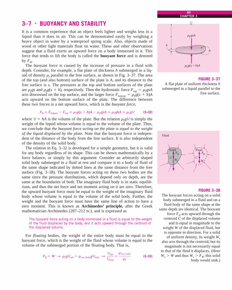
3–7 ! BUOYANCY AND STABILITYIt is a common experience that an object feels lighter and weighs less in aliquid than it does in air. This can be demonstrated easily by weighing aheavy object in water by a waterproof spring scale. Also, objects made ofwood or other light materials float on water. These and other observationssuggest that a fluid exerts an upward force on a body immersed in it. Thisforce that tends to lift the body is called the buoyant force and is denotedby FB.

The buoyant force is caused by the increase of pressure in a fluid withdepth. Consider, for example, a flat plate of thickness h submerged in a liq-uid of density rf parallel to the free surface, as shown in Fig. 3–37. The areaof the top (and also bottom) surface of the plate is A, and its distance to thefree surface is s. The pressures at the top and bottom surfaces of the plateare rfgs and rfg(s ! h), respectively. Then the hydrostatic force Ftop " rfgsAacts downward on the top surface, and the larger force Fbottom " rfg(s ! h)Aacts upward on the bottom surface of the plate. The difference betweenthese two forces is a net upward force, which is the buoyant force,

(3–32)

where V " hA is the volume of the plate. But the relation rfgV is simply theweight of the liquid whose volume is equal to the volume of the plate. Thus,we conclude that the buoyant force acting on the plate is equal to the weightof the liquid displaced by the plate. Note that the buoyant force is indepen-dent of the distance of the body from the free surface. It is also independentof the density of the solid body.

The relation in Eq. 3–32 is developed for a simple geometry, but it is validfor any body regardless of its shape. This can be shown mathematically by aforce balance, or simply by this argument: Consider an arbitrarily shapedsolid body submerged in a fluid at rest and compare it to a body of fluid ofthe same shape indicated by dotted lines at the same distance from the freesurface (Fig. 3–38). The buoyant forces acting on these two bodies are thesame since the pressure distributions, which depend only on depth, are thesame at the boundaries of both. The imaginary fluid body is in static equilib-rium, and thus the net force and net moment acting on it are zero. Therefore,the upward buoyant force must be equal to the weight of the imaginary fluidbody whose volume is equal to the volume of the solid body. Further, theweight and the buoyant force must have the same line of action to have azero moment. This is known as Archimedes’ principle, after the Greekmathematician Archimedes (287–212 BC), and is expressed as

The buoyant force acting on a body immersed in a fluid is equal to the weightof the fluid displaced by the body, and it acts upward through the centroid ofthe displaced volume.

For floating bodies, the weight of the entire body must be equal to thebuoyant force, which is the weight of the fluid whose volume is equal to thevolume of the submerged portion of the floating body. That is,

(3–33)FB " W ! rf gVsub " rave, bodygVtotal ! Vsub

Vtotal"rave, body

rf

FB " Fbottom # Ftop " rf g(s ! h)A # rf gsA " rf ghA " rf gV

89CHAPTER 3

rf gsAs

h

rf g(s + h)A

A

FIGURE 3–37A flat plate of uniform thickness h

submerged in a liquid parallel to thefree surface.

Fluid

FluidSolid

Ws

FB FB

WCC

FIGURE 3–38The buoyant forces acting on a solidbody submerged in a fluid and on afluid body of the same shape at the

same depth are identical. The buoyantforce FB acts upward through the

centroid C of the displaced volumeand is equal in magnitude to the

weight W of the displaced fluid, but is opposite in direction. For a solid

of uniform density, its weight Wsalso acts through the centroid, but its

magnitude is not necessarily equal to that of the fluid it displaces. (HereWs % W and thus Ws % FB; this solid

body would sink.)

cen72367_ch03.qxd 10/29/04 2:21 PM Page 89

Therefore, the submerged volume fraction of a floating body is equal to theratio of the average density of the body to the density of the fluid. Note thatwhen the density ratio is equal to or greater than one, the floating bodybecomes completely submerged.

It follows from these discussions that a body immersed in a fluid (1) remainsat rest at any point in the fluid when its density is equal to the density of thefluid, (2) sinks to the bottom when its density is greater than the density ofthe fluid, and (3) rises to the surface of the fluid and floats when the densityof the body is less than the density of the fluid (Fig. 3–39).

The buoyant force is proportional to the density of the fluid, and thus wemight think that the buoyant force exerted by gases such as air is negligible.This is certainly the case in general, but there are significant exceptions. Forexample, the volume of a person is about 0.1 m3, and taking the density ofair to be 1.2 kg/m3, the buoyant force exerted by air on the person is

The weight of an 80-kg person is 80 ( 9.81 " 788 N. Therefore, ignoringthe buoyancy in this case results in an error in weight of just 0.15 percent,which is negligible. But the buoyancy effects in gases dominate some impor-tant natural phenomena such as the rise of warm air in a cooler environmentand thus the onset of natural convection currents, the rise of hot-air or heliumballoons, and air movements in the atmosphere. A helium balloon, for exam-ple, rises as a result of the buoyancy effect until it reaches an altitude wherethe density of air (which decreases with altitude) equals the density ofhelium in the balloon—assuming the balloon does not burst by then, andignoring the weight of the balloon’s skin.

Archimedes’ principle is also used in modern geology by considering thecontinents to be floating on a sea of magma.

EXAMPLE 3–10 Measuring Specific Gravity by a Hydrometer

If you have a seawater aquarium, you have probably used a small cylindricalglass tube with some lead-weight at its bottom to measure the salinity of thewater by simply watching how deep the tube sinks. Such a device that floatsin a vertical position and is used to measure the specific gravity of a liquidis called a hydrometer (Fig. 3–40). The top part of the hydrometer extends

FB " rf gV " (1.2 kg&m3)(9.81 m&s2)(0.1 m3) " 1.2 N

90FLUID MECHANICS

Fluid

Sinkingbody

Suspended body (neutrally buoyant)

Floatingbody r < rf

r = rf

r > rfrf

FIGURE 3–39A solid body dropped into a fluid willsink, float, or remain at rest at any pointin the fluid, depending on its densityrelative to the density of the fluid.

cen72367_ch03.qxd 10/29/04 2:21 PM Page 90

above the liquid surface, and the divisions on it allow one to read the spe-cific gravity directly. The hydrometer is calibrated such that in pure water itreads exactly 1.0 at the air–water interface. (a) Obtain a relation for the spe-cific gravity of a liquid as a function of distance $z from the mark corre-sponding to pure water and (b) determine the mass of lead that must bepoured into a 1-cm-diameter, 20-cm-long hydrometer if it is to float halfway(the 10-cm mark) in pure water.

SOLUTION The specific gravity of a liquid is to be measured by a hydrome-ter. A relation between specific gravity and the vertical distance from the ref-erence level is to be obtained, and the amount of lead that needs to beadded into the tube for a certain hydrometer is to be determined.Assumptions 1 The weight of the glass tube is negligible relative to theweight of the lead added. 2 The curvature of the tube bottom is disregarded.Properties We take the density of pure water to be 1000 kg/m3.Analysis (a) Noting that the hydrometer is in static equilibrium, the buoyantforce FB exerted by the liquid must always be equal to the weight W of thehydrometer. In pure water, let the vertical distance between the bottom ofthe hydrometer and the free surface of water be z0. Setting FB " W in thiscase gives

(1)

where A is the cross-sectional area of the tube, and rw is the density of purewater.

In a fluid lighter than water (rf * rw), the hydrometer will sink deeper, andthe liquid level will be a distance of $z above z0. Again setting FB " W gives

(2)

This relation is also valid for fluids heavier than water by taking the $z belowz0 to be a negative quantity. Setting Eqs. (1) and (2) here equal to eachother since the weight of the hydrometer is constant and rearranging gives

which is the relation between the specific gravity of the fluid and $z. Notethat z0 is constant for a given hydrometer and $z is negative for fluids heav-ier than pure water.

(b) Disregarding the weight of the glass tube, the amount of lead that needsto be added to the tube is determined from the requirement that the weightof the lead be equal to the buoyant force. When the hydrometer is floatingwith half of it submerged in water, the buoyant force acting on it is

Equating FB to the weight of lead gives

Solving for m and substituting, the mass of lead is determined to be

Discussion Note that if the hydrometer were required to sink only 5 cm inwater, the required mass of lead would be one-half of this amount. Also, theassumption that the weight of the glass tube is negligible needs to bechecked since the mass of lead is only 7.85 g.

m " rwVsub " rw(pR2hsub) " (1000 kg&m3)[p(0.005 m)2(0.1 m)] " 0.00785 kg

W " mg " rw gVsub

FB " rwgVsub

rw gAz0 " rf gA(z0 ! $z) ! SGf "rf

rw"

z0

z0 ! $z

Whydro " FB, f " rf gVsub " rf gA(z0 ! $z)

Whydro " FB, w " rw gVsub " rw gAz0

91CHAPTER 3

Hydrometer

Lead

1.0

W

FB

z0

%z

FIGURE 3–40Schematic for Example 3–10.

cen72367_ch03.qxd 10/29/04 2:21 PM Page 91

EXAMPLE 3–11 Weight Loss of an Object in Seawater

A crane is used to lower weights into the sea (density " 1025 kg/m3) for anunderwater construction project (Fig. 3–41). Determine the tension in therope of the crane due to a rectangular 0.4-m ( 0.4-m ( 3-m concrete block(density " 2300 kg/m3) when it is (a) suspended in the air and (b) com-pletely immersed in water.

SOLUTION A concrete block is lowered into the sea. The tension in therope is to be determined before and after the block is in water.Assumptions 1 The buoyancy of air is negligible. 2 The weight of the ropesis negligible.Properties The densities are given to be 1025 kg/m3 for seawater and2300 kg/m3 for concrete.Analysis (a) Consider the free-body diagram of the concrete block. Theforces acting on the concrete block in air are its weight and the upward pullaction (tension) by the rope. These two forces must balance each other, andthus the tension in the rope must be equal to the weight of the block:

(b) When the block is immersed in water, there is the additional force ofbuoyancy acting upward. The force balance in this case gives

Discussion Note that the weight of the concrete block, and thus the tensionof the rope, decreases by (10.8 # 6.0)/10.8 " 55 percent in water.

Stability of Immersed and Floating BodiesAn important application of the buoyancy concept is the assessment of thestability of immersed and floating bodies with no external attachments. Thistopic is of great importance in the design of ships and submarines (Fig.3–42). Here we provide some general qualitative discussions on vertical androtational stability.

We use the “ball on the floor” analogy to explain the fundamental conceptsof stability and instability. Shown in Fig. 3–43 are three balls at rest on thefloor. Case (a) is stable since any small disturbance (someone moves the ballto the right or left) generates a restoring force (due to gravity) that returns itto its initial position. Case (b) is neutrally stable because if someone movesthe ball to the right or left, it would stay put at its new location. It has no ten-dency to move back to its original location, nor does it continue to move

FT, water " W # FB " 10.8 # 4.8 " 6.0 kN

FB " rf gV "(1025 kg&m3)(9.81 m&s2)(0.48 m3)a 1 kN1000 kg ' m&s2b " 4.8 kN

" (2300 kg&m3)(9.81 m&s2)(0.48 m3)a 1 kN1000 kg ' m&s2b " 10.8 kN

FT, air " W " rconcrete gV

V " (0.4 m)(0.4 m)(3 m) " 0.48 m3

92FLUID MECHANICS

FB

FT, water

W

Water

FT, air

W

Concreteblock

Air

Rope

FIGURE 3–41Schematic for Example 3–11.

cen72367_ch03.qxd 10/29/04 2:21 PM Page 92

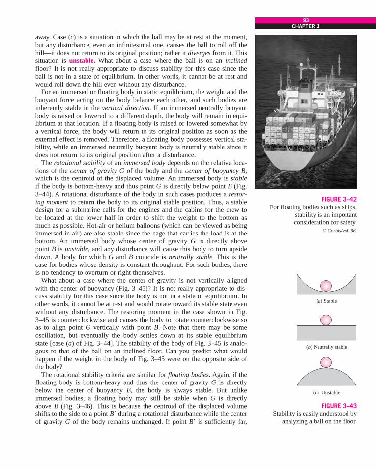
away. Case (c) is a situation in which the ball may be at rest at the moment,but any disturbance, even an infinitesimal one, causes the ball to roll off thehill—it does not return to its original position; rather it diverges from it. Thissituation is unstable. What about a case where the ball is on an inclinedfloor? It is not really appropriate to discuss stability for this case since theball is not in a state of equilibrium. In other words, it cannot be at rest andwould roll down the hill even without any disturbance.

For an immersed or floating body in static equilibrium, the weight and thebuoyant force acting on the body balance each other, and such bodies areinherently stable in the vertical direction. If an immersed neutrally buoyantbody is raised or lowered to a different depth, the body will remain in equi-librium at that location. If a floating body is raised or lowered somewhat bya vertical force, the body will return to its original position as soon as theexternal effect is removed. Therefore, a floating body possesses vertical sta-bility, while an immersed neutrally buoyant body is neutrally stable since itdoes not return to its original position after a disturbance.

The rotational stability of an immersed body depends on the relative loca-tions of the center of gravity G of the body and the center of buoyancy B,which is the centroid of the displaced volume. An immersed body is stableif the body is bottom-heavy and thus point G is directly below point B (Fig.3–44). A rotational disturbance of the body in such cases produces a restor-ing moment to return the body to its original stable position. Thus, a stabledesign for a submarine calls for the engines and the cabins for the crew tobe located at the lower half in order to shift the weight to the bottom asmuch as possible. Hot-air or helium balloons (which can be viewed as beingimmersed in air) are also stable since the cage that carries the load is at thebottom. An immersed body whose center of gravity G is directly abovepoint B is unstable, and any disturbance will cause this body to turn upsidedown. A body for which G and B coincide is neutrally stable. This is thecase for bodies whose density is constant throughout. For such bodies, thereis no tendency to overturn or right themselves.

What about a case where the center of gravity is not vertically alignedwith the center of buoyancy (Fig. 3–45)? It is not really appropriate to dis-cuss stability for this case since the body is not in a state of equilibrium. Inother words, it cannot be at rest and would rotate toward its stable state evenwithout any disturbance. The restoring moment in the case shown in Fig.3–45 is counterclockwise and causes the body to rotate counterclockwise soas to align point G vertically with point B. Note that there may be someoscillation, but eventually the body settles down at its stable equilibriumstate [case (a) of Fig. 3–44]. The stability of the body of Fig. 3–45 is analo-gous to that of the ball on an inclined floor. Can you predict what wouldhappen if the weight in the body of Fig. 3–45 were on the opposite side ofthe body?

The rotational stability criteria are similar for floating bodies. Again, if thefloating body is bottom-heavy and thus the center of gravity G is directlybelow the center of buoyancy B, the body is always stable. But unlikeimmersed bodies, a floating body may still be stable when G is directlyabove B (Fig. 3–46). This is because the centroid of the displaced volumeshifts to the side to a point B+ during a rotational disturbance while the centerof gravity G of the body remains unchanged. If point B+ is sufficiently far,

93CHAPTER 3

(a) Stable

(b) Neutrally stable

(c) Unstable

FIGURE 3–43Stability is easily understood by

analyzing a ball on the floor.

FIGURE 3–42For floating bodies such as ships,

stability is an important consideration for safety.

© Corbis/vol. 96.

cen72367_ch03.qxd 10/29/04 2:21 PM Page 93

these two forces create a restoring moment and return the body to the origi-nal position. A measure of stability for floating bodies is the metacentricheight GM, which is the distance between the center of gravity G and themetacenter M—the intersection point of the lines of action of the buoyantforce through the body before and after rotation. The metacenter may beconsidered to be a fixed point for most hull shapes for small rolling anglesup to about 20°. A floating body is stable if point M is above point G, andthus GM is positive, and unstable if point M is below point G, and thus GMis negative. In the latter case, the weight and the buoyant force acting on thetilted body generate an overturning moment instead of a restoring moment,causing the body to capsize. The length of the metacentric height GM aboveG is a measure of the stability: the larger it is, the more stable is the floatingbody.

As already discussed, a boat can tilt to some maximum angle without cap-sizing, but beyond that angle it overturns (and sinks). We make a final anal-ogy between the stability of floating objects and the stability of a ballrolling along the floor. Namely, imagine the ball in a trough between twohills (Fig. 3–47). The ball returns to its stable equilibrium position afterbeing perturbed—up to a limit. If the perturbation amplitude is too great,the ball rolls down the opposite side of the hill and does not return to itsequilibrium position. This situation is described as stable up to some limit-ing level of disturbance, but unstable beyond.

94FLUID MECHANICS

Restoring moment

Weight

FB

B

W

G

FIGURE 3–45When the center of gravity G of animmersed neutrally buoyant body isnot vertically aligned with the centerof buoyancy B of the body, it is not inan equilibrium state and would rotateto its stable state, even without anydisturbance.

FluidWeight

Weight(a) Stable (b) Neutrally stable (c) Unstable

FB FB

FB

B B BGW W

WG

G

Metacenter

Restoringmoment

(a) Stable (b) Stable (c) Unstable

WG G

B B!

M

FB

Overturningmoment

G

B!!M

FIGURE 3–44An immersed neutrally buoyant bodyis (a) stable if the center of gravity G is directly below the center ofbuoyancy B of the body, (b) neutrallystable if G and B are coincident, and(c) unstable if G is directly above B.

FIGURE 3–46A floating body is stable if the body isbottom-heavy and thus the center ofgravity G is below the centroid B ofthe body, or if the metacenter M isabove point G. However, the body isunstable if point M is below point G.

cen72367_ch03.qxd 11/16/04 12:10 PM Page 94

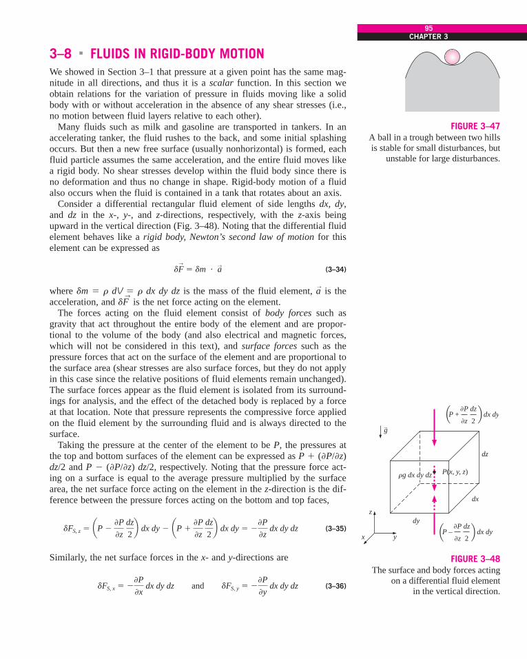
3–8 ! FLUIDS IN RIGID-BODY MOTIONWe showed in Section 3–1 that pressure at a given point has the same mag-nitude in all directions, and thus it is a scalar function. In this section weobtain relations for the variation of pressure in fluids moving like a solidbody with or without acceleration in the absence of any shear stresses (i.e.,no motion between fluid layers relative to each other).

Many fluids such as milk and gasoline are transported in tankers. In anaccelerating tanker, the fluid rushes to the back, and some initial splashingoccurs. But then a new free surface (usually nonhorizontal) is formed, eachfluid particle assumes the same acceleration, and the entire fluid moves likea rigid body. No shear stresses develop within the fluid body since there isno deformation and thus no change in shape. Rigid-body motion of a fluidalso occurs when the fluid is contained in a tank that rotates about an axis.

Consider a differential rectangular fluid element of side lengths dx, dy,and dz in the x-, y-, and z-directions, respectively, with the z-axis beingupward in the vertical direction (Fig. 3–48). Noting that the differential fluidelement behaves like a rigid body, Newton’s second law of motion for thiselement can be expressed as

(3–34)

where dm " r dV " r dx dy dz is the mass of the fluid element, a!

is theacceleration, and dF

!is the net force acting on the element.

The forces acting on the fluid element consist of body forces such asgravity that act throughout the entire body of the element and are propor-tional to the volume of the body (and also electrical and magnetic forces,which will not be considered in this text), and surface forces such as thepressure forces that act on the surface of the element and are proportional tothe surface area (shear stresses are also surface forces, but they do not applyin this case since the relative positions of fluid elements remain unchanged).The surface forces appear as the fluid element is isolated from its surround-ings for analysis, and the effect of the detached body is replaced by a forceat that location. Note that pressure represents the compressive force appliedon the fluid element by the surrounding fluid and is always directed to thesurface.

Taking the pressure at the center of the element to be P, the pressures atthe top and bottom surfaces of the element can be expressed as P ! (,P/,z)dz/2 and P # (,P/,z) dz/2, respectively. Noting that the pressure force act-ing on a surface is equal to the average pressure multiplied by the surfacearea, the net surface force acting on the element in the z-direction is the dif-ference between the pressure forces acting on the bottom and top faces,

(3–35)

Similarly, the net surface forces in the x- and y-directions are

(3–36)dFS, x " #,P,x

dx dy dz and dFS, y " #,P,y

dx dy dz

dFS, z " aP #,P,z

dz2b dx dy # aP !

,P,z

dz2b dx dy " #

,P,z

dx dy dz

dF!

" dm ' a!

95CHAPTER 3

FIGURE 3–47A ball in a trough between two hills is stable for small disturbances, but

unstable for large disturbances.

dx

dz

dy

P(x, y, z)

yx

z

rg dx dy dz

P + dx dy,P

,z

dz

2RQ

RQP – dx dy,P

,z

dz

2

g

FIGURE 3–48The surface and body forces acting

on a differential fluid element in the vertical direction.

cen72367_ch03.qxd 10/29/04 2:21 PM Page 95

Then the surface force (which is simply the pressure force) acting on theentire element can be expressed in vector form as

(3–37)

where i!

, j!

, and k!

are the unit vectors in the x-, y-, and z-directions, respec-tively, and

(3–38)

is the pressure gradient. Note that the -!

or “del” is a vector operator that isused to express the gradients of a scalar function compactly in vector form.Also, the gradient of a scalar function is expressed in a given direction andthus it is a vector quantity.

The only body force acting on the fluid element is the weight of the ele-ment acting in the negative z-direction, and it is expressed as dFB, z " #gdm" #rg dx dy dz or in vector form as

(3–39)

Then the total force acting on the element becomes

(3–40)

Substituting into Newton’s second law of motion dF!

" dm ' a!

" r dx dy dz' a

!and canceling dx dy dz, the general equation of motion for a fluid that

acts as a rigid body (no shear stresses) is determined to be

Rigid-body motion of fluids: (3–41)

Resolving the vectors into their components, this relation can be expressedmore explicitly as

(3–42)

or, in scalar form in the three orthogonal directions, as

Accelerating fluids: (3–43)

where ax, ay, and az are accelerations in the x-, y-, and z-directions, respec-tively.

Special Case 1: Fluids at RestFor fluids at rest or moving on a straight path at constant velocity, all com-ponents of acceleration are zero, and the relations in Eqs. 3–43 reduce to

Fluids at rest: (3–44)

which confirm that, in fluids at rest, the pressure remains constant in anyhorizontal direction (P is independent of x and y) and varies only in the ver-tical direction as a result of gravity [and thus P " P(z)]. These relations areapplicable for both compressible and incompressible fluids.

,P,x

" 0, ,P,y

" 0, and dPdz

" #rg

,P,x

" #rax, ,P,y

" #ray, and ,P,z

" #r(g ! az)

,P,x

i!

!,P,y

j!

!,P,z

k!

! rgk!

" #r(ax i!

! ay j!

! az k!

)

§!

P ! rgk!

" #ra!

dF!

" dF!

S ! dF!

B " #(§!

P ! rgk!) dx dy dz

dF!

B, z " #gdmk!

" #rg dx dy dzk!

§!

P ",P,x

i!

!,P,y

j!

!,P,z

k!

" #a,P,x

i!

!,P,y

j!

!,P,z

k!b dx dy dz " #§

!P dx dy dz

dF!

S " dFS, x i!

! dFS, y j!

! dFS, z k!

96FLUID MECHANICS

cen72367_ch03.qxd 10/29/04 2:22 PM Page 96

Special Case 2: Free Fall of a Fluid BodyA freely falling body accelerates under the influence of gravity. When theair resistance is negligible, the acceleration of the body equals the gravita-tional acceleration, and acceleration in any horizontal direction is zero.Therefore, ax " ay " 0 and az " #g. Then the equations of motion foraccelerating fluids (Eqs. 3–43) reduce to

Free-falling fluids: (3–45)

Therefore, in a frame of reference moving with the fluid, it behaves like it isin an environment with zero gravity. Also, the gage pressure in a drop ofliquid in free fall is zero throughout. (Actually, the gage pressure is slightlyabove zero due to surface tension, which holds the drop intact.)

When the direction of motion is reversed and the fluid is forced to accel-erate vertically with az " !g by placing the fluid container in an elevator ora space vehicle propelled upward by a rocket engine, the pressure gradientin the z-direction is ,P/,z " #2rg. Therefore, the pressure difference acrossa fluid layer now doubles relative to the stationary fluid case (Fig. 3–49).

Acceleration on a Straight PathConsider a container partially filled with a liquid. The container is movingon a straight path with a constant acceleration. We take the projection of thepath of motion on the horizontal plane to be the x-axis, and the projectionon the vertical plane to be the z-axis, as shown in Fig. 3–50. The x- and z-components of acceleration are ax and az. There is no movement in the y-direction, and thus the acceleration in that direction is zero, ay " 0. Thenthe equations of motion for accelerating fluids (Eqs. 3–43) reduce to

(3–46)

Therefore, pressure is independent of y. Then the total differential of P" P(x, z), which is (,P/,x) dx ! (,P/,z) dz, becomes

(3–47)

For r " constant, the pressure difference between two points 1 and 2 in thefluid is determined by integration to be

(3–48)

Taking point 1 to be the origin (x " 0, z " 0) where the pressure is P0 andpoint 2 to be any point in the fluid (no subscript), the pressure distributioncan be expressed as

Pressure variation: (3–49)

The vertical rise (or drop) of the free surface at point 2 relative to point 1can be determined by choosing both 1 and 2 on the free surface (so that P1" P2), and solving Eq. 3–48 for z2 # z1 (Fig. 3–51),

Vertical rise of surface: (3–50)$zs " zs2 # zs1 " #ax

g ! az (x2 # x1)

P " P0 # raxx # r(g ! az)z

P2 # P1 " #rax(x2 # x1) # r(g ! az)(z2 # z1)

dP " #rax dx # r(g ! az) dz

,P,x

" #rax, ,P,y

" 0, and ,P,z

" #r(g ! az)

,P,x

",P,y

",P,z

" 0 ! P " constant

97CHAPTER 3

az = –g

z z

az = g

P2 = P1

P1 P1

P2 = P1 + 2rgh

(a) Free fall of aliquid

(b) Upward accelerationof a liquid with az = +g

Liquid, rLiquid, rh h

FIGURE 3–49The effect of acceleration on the

pressure of a liquid during free fall and upward acceleration.

$zmax

z

x

b

ho

aza

g

ax

Liquid

Freesurface

u

FIGURE 3–50Rigid-body motion of a liquid in a

linearly accelerating tank.

cen72367_ch03.qxd 10/29/04 2:22 PM Page 97

where zs is the z-coordinate of the liquid’s free surface. The equation forsurfaces of constant pressure, called isobars, is obtained from Eq. 3–47 bysetting d P " 0 and replacing z by zisobar, which is the z-coordinate (the ver-tical distance) of the surface as a function of x. It gives

Surfaces of constant pressure: (3–51)

Thus we conclude that the isobars (including the free surface) in an incom-pressible fluid with constant acceleration in linear motion are parallel sur-faces whose slope in the xz-plane is

Slope of isobars: (3–52)

Obviously, the free surface of such a fluid is a plane surface, and it isinclined unless ax " 0 (the acceleration is in the vertical direction only).Also, the conservation of mass together with the assumption of incompress-ibility (r " constant) requires that the volume of the fluid remain constantbefore and during acceleration. Therefore, the rise of fluid level on one sidemust be balanced by a drop of fluid level on the other side.

EXAMPLE 3–12 Overflow from a Water Tank During Acceleration

An 80-cm-high fish tank of cross section 2 m ( 0.6 m that is initially filledwith water is to be transported on the back of a truck (Fig. 3–52). The truckaccelerates from 0 to 90 km/h in 10 s. If it is desired that no water spillsduring acceleration, determine the allowable initial water height in the tank.Would you recommend the tank to be aligned with the long or short side par-allel to the direction of motion?

SOLUTION A fish tank is to be transported on a truck. The allowable waterheight to avoid spill of water during acceleration and the proper orientationare to be determined.Assumptions 1 The road is horizontal during acceleration so that accelera-tion has no vertical component (az " 0). 2 Effects of splashing, braking, dri-ving over bumps, and climbing hills are assumed to be secondary and arenot considered. 3 The acceleration remains constant.Analysis We take the x-axis to be the direction of motion, the z-axis to bethe upward vertical direction, and the origin to be the lower left corner of thetank. Noting that the truck goes from 0 to 90 km/h in 10 s, the accelerationof the truck is

The tangent of the angle the free surface makes with the horizontal is

tan u "ax

g ! az"

2.59.81 ! 0

" 0.255 (and thus u" 14.3))

ax "$V$t

"(90 # 0) km&h

10 sa 1 m&s3.6 km&h

b " 2.5 m&s2

Slope "dzisobar

dx" #

ax

g ! az" #tan u

dzisobar

dx" #

ax

g ! az" constant

98FLUID MECHANICS

$zs = zs2 – zs1

x1 – x2

aza

g

ax

Constantpressurelines

Freesurface2

1

z

x

u

FIGURE 3–51Lines of constant pressure (which are the projections of the surfaces ofconstant pressure on the xz-plane) in a linearly accelerating liquid, and thevertical rise.

$zs

ax

b

Watertank

80 cm

u

FIGURE 3–52Schematic for Example 3–12.

cen72367_ch03.qxd 10/29/04 2:22 PM Page 98

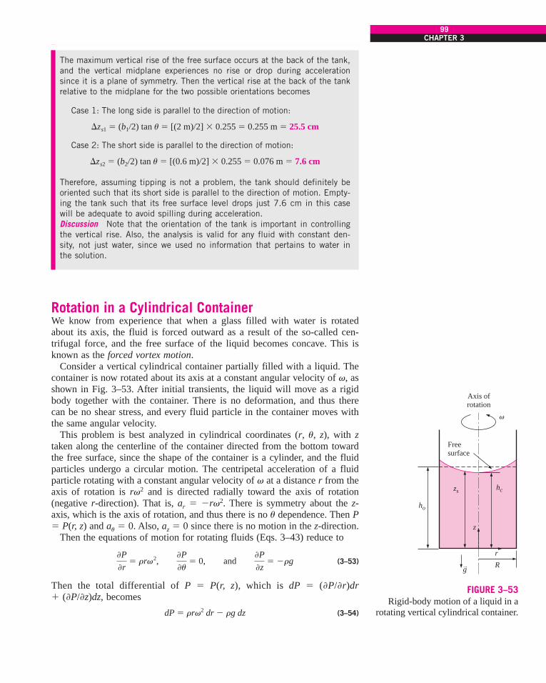
The maximum vertical rise of the free surface occurs at the back of the tank,and the vertical midplane experiences no rise or drop during accelerationsince it is a plane of symmetry. Then the vertical rise at the back of the tankrelative to the midplane for the two possible orientations becomes

Case 1: The long side is parallel to the direction of motion:

Case 2: The short side is parallel to the direction of motion:

Therefore, assuming tipping is not a problem, the tank should definitely beoriented such that its short side is parallel to the direction of motion. Empty-ing the tank such that its free surface level drops just 7.6 cm in this casewill be adequate to avoid spilling during acceleration.Discussion Note that the orientation of the tank is important in controllingthe vertical rise. Also, the analysis is valid for any fluid with constant den-sity, not just water, since we used no information that pertains to water inthe solution.

Rotation in a Cylindrical ContainerWe know from experience that when a glass filled with water is rotatedabout its axis, the fluid is forced outward as a result of the so-called cen-trifugal force, and the free surface of the liquid becomes concave. This isknown as the forced vortex motion.

Consider a vertical cylindrical container partially filled with a liquid. Thecontainer is now rotated about its axis at a constant angular velocity of v, asshown in Fig. 3–53. After initial transients, the liquid will move as a rigidbody together with the container. There is no deformation, and thus therecan be no shear stress, and every fluid particle in the container moves withthe same angular velocity.

This problem is best analyzed in cylindrical coordinates (r, u, z), with ztaken along the centerline of the container directed from the bottom towardthe free surface, since the shape of the container is a cylinder, and the fluidparticles undergo a circular motion. The centripetal acceleration of a fluidparticle rotating with a constant angular velocity of v at a distance r from theaxis of rotation is rv2 and is directed radially toward the axis of rotation(negative r-direction). That is, ar " #rv2. There is symmetry about the z-axis, which is the axis of rotation, and thus there is no u dependence. Then P" P(r, z) and au " 0. Also, az " 0 since there is no motion in the z-direction.

Then the equations of motion for rotating fluids (Eqs. 3–43) reduce to

(3–53)

Then the total differential of P " P(r, z), which is dP " (,P/,r)dr! (,P/,z)dz, becomes

(3–54)dP " rrv2 dr # rg dz

,P,r

" rrv2, ,P,u

" 0, and ,P,z

" #rg

$zs2 " (b2&2) tan u" [(0.6 m)&2] ( 0.255 " 0.076 m " 7.6 cm

$zs1 " (b1&2) tan u" [(2 m)&2] ( 0.255 " 0.255 m " 25.5 cm

99CHAPTER 3

ho

zs

z

Axis ofrotation

Freesurface

R

r

g

hc

v

FIGURE 3–53Rigid-body motion of a liquid in a

rotating vertical cylindrical container.

cen72367_ch03.qxd 10/29/04 2:22 PM Page 99

The equation for surfaces of constant pressure is obtained by setting dP " 0and replacing z by zisobar, which is the z-value (the vertical distance) of thesurface as a function of r. It gives

(3–55)

Integrating, the equation for the surfaces of constant pressure is determinedto be

Surfaces of constant pressure: (3–56)

which is the equation of a parabola. Thus we conclude that the surfaces ofconstant pressure, including the free surface, are paraboloids of revolution(Fig. 3–54).

The value of the integration constant C1 is different for different parabo-loids of constant pressure (i.e., for different isobars). For the free surface,setting r " 0 in Eq. 3–56 gives zisobar(0) " C1 " hc, where hc is the distanceof the free surface from the bottom of the container along the axis of rota-tion (Fig. 3–53). Then the equation for the free surface becomes

(3–57)

where zs is the distance of the free surface from the bottom of the containerat radius r. The underlying assumption in this analysis is that there is suffi-cient liquid in the container so that the entire bottom surface remains cov-ered with liquid.

The volume of a cylindrical shell element of radius r, height zs, and thick-ness dr is dV " 2przs dr. Then the volume of the paraboloid formed by thefree surface is

(3–58)

Since mass is conserved and density is constant, this volume must be equalto the original volume of the fluid in the container, which is

(3–59)

where h0 is the original height of the fluid in the container with no rotation.Setting these two volumes equal to each other, the height of the fluid alongthe centerline of the cylindrical container becomes

(3–60)

Then the equation of the free surface becomes

Free surface: (3–61)

The maximum vertical height occurs at the edge where r " R, and the max-imum height difference between the edge and the center of the free surface

zs " h0 #v2

4g (R2 # 2r 2)

hc " h0 #v2R2

4g

V " pR2h0

V " !R

r"0

2pzsr dr " 2p !R

r"0

av2

2g r 2 ! hcbr dr " pR2av2R2

4g! hcb

zs "v2

2g r2 ! hc

zisobar "v2

2g r 2 ! C1

dzisobar

dr"

rv2

g

100FLUID MECHANICS

P7

Freesurface

P6

P5

P4

P3

P2

P1$zs, max

v

FIGURE 3–54Surfaces of constant pressure in arotating liquid.

cen72367_ch03.qxd 10/29/04 2:22 PM Page 100

is determined by evaluating zs at r " R and also at r " 0, and taking theirdifference,

Maximum height difference: (3–62)

When r " constant, the pressure difference between two points 1 and 2 inthe fluid is determined by integrating dP " rrv2 dr # rg dz. This yields

(3–63)

Taking point 1 to be the origin (r " 0, z " 0) where the pressure is P0 andpoint 2 to be any point in the fluid (no subscript), the pressure distributioncan be expressed as

Pressure variation: (3–64)

Note that at a fixed radius, the pressure varies hydrostatically in the verticaldirection, as in a fluid at rest. For a fixed vertical distance z, the pressurevaries with the square of the radial distance r, increasing from the centerlinetoward the outer edge. In any horizontal plane, the pressure differencebetween the center and edge of the container of radius R is $P " rv2R2/2.

EXAMPLE 3–13 Rising of a Liquid During Rotation

A 20-cm-diameter, 60-cm-high vertical cylindrical container, shown in Fig.3–55, is partially filled with 50-cm-high liquid whose density is 850 kg/m3.Now the cylinder is rotated at a constant speed. Determine the rotationalspeed at which the liquid will start spilling from the edges of the container.

SOLUTION A vertical cylindrical container partially filled with a liquid isrotated. The angular speed at which the liquid will start spilling is to bedetermined.Assumptions 1 The increase in the rotational speed is very slow so that theliquid in the container always acts as a rigid body. 2 The bottom surface ofthe container remains covered with liquid during rotation (no dry spots).Analysis Taking the center of the bottom surface of the rotating verticalcylinder as the origin (r " 0, z " 0), the equation for the free surface of theliquid is given as

Then the vertical height of the liquid at the edge of the container where r "R becomes

where h0 " 0.5 m is the original height of the liquid before rotation. Justbefore the liquid starts spilling, the height of the liquid at the edge of the con-tainer equals the height of the container, and thus zs (R) " 0.6 m. Solving the

zs(R) " h0 !v2R2

4g

zs " h0 #v2

4g (R2 # 2r 2)

P " P0 !rv2

2 r 2 # rgz

P2 # P1 "rv2

2 (r 2

2 # r 21) # rg(z2 # z1)

$zs, max " zs(R) # zs(0) "v2

2g R2

101CHAPTER 3

h0

zs

Freesurface

R

r

g

z

v

FIGURE 3–55Schematic for Example 3–13.

cen72367_ch03.qxd 10/29/04 2:22 PM Page 101

last equation for v and substituting, the maximum rotational speed of thecontainer is determined to be

Noting that one complete revolution corresponds to 2p rad, the rotationalspeed of the container can also be expressed in terms of revolutions perminute (rpm) as

Therefore, the rotational speed of this container should be limited to 189rpm to avoid any spill of liquid as a result of the centrifugal effect.Discussion Note that the analysis is valid for any liquid since the result isindependent of density or any other fluid property. We should also verify thatour assumption of no dry spots is valid. The liquid height at the center is

Since zs(0) is positive, our assumption is validated.

zs(0) " h0 #v2R2

4g" 0.4 m

n#

"v

2p"

19.8 rad&s2p rad&rev

a 60 s1 min

b " 189 rpm

v "B4g[zs(R) # h0]

R2 "B4(9.81 m&s2)[(0.6 # 0.5) m](0.1 m)2 " 19.8 rad&s

102FLUID MECHANICS

SUMMARY

The normal force exerted by a fluid per unit area is calledpressure, and its unit is the pascal, 1 Pa # 1 N/m2. The pres-sure relative to absolute vacuum is called the absolute pres-sure, and the difference between the absolute pressure andthe local atmospheric pressure is called the gage pressure.Pressures below atmospheric pressure are called vacuumpressures. The absolute, gage, and vacuum pressures arerelated by

The pressure at a point in a fluid has the same magnitude inall directions. The variation of pressure with elevation in afluid at rest is given by

where the positive z-direction is taken to be upward. Whenthe density of the fluid is constant, the pressure differenceacross a fluid layer of thickness $z is

The absolute and gage pressures in a static liquid open to theatmosphere at a depth h from the free surface are

P " Patm ! rgh and Pgage " rgh

$P " P2 # P1 " rg $z

dPdz

" #rg

Pvac " Patm # Pabs

Pgage " Pabs # Patm

The pressure in a fluid at rest remains constant in the hori-zontal direction. Pascal’s law states that the pressure appliedto a confined fluid increases the pressure throughout by thesame amount. The atmospheric pressure is measured by abarometer and is given by

where h is the height of the liquid column.Fluid statics deals with problems associated with fluids at

rest, and it is called hydrostatics when the fluid is a liquid.The magnitude of the resultant force acting on a plane sur-face of a completely submerged plate in a homogeneous fluidis equal to the product of the pressure PC at the centroid ofthe surface and the area A of the surface and is expressed as

where hC " yC sin u is the vertical distance of the centroidfrom the free surface of the liquid. The pressure P0 is usuallythe atmospheric pressure, which cancels out in most casessince it acts on both sides of the plate. The point of intersec-tion of the line of action of the resultant force and the surfaceis the center of pressure. The vertical location of the line ofaction of the resultant force is given by

yP " yC !Ixx, C

[yC ! P0 &(rg sin u)]A

FR " (P0 ! rghC)A " PC A " Pave A

Patm " rgh

cen72367_ch03.qxd 10/29/04 2:22 PM Page 102

CHAPTER 3103

where Ixx, C is the second moment of area about the x-axispassing through the centroid of the area.

A fluid exerts an upward force on a body immersed in it.This force is called the buoyant force and is expressed as

where V is the volume of the body. This is known asArchimedes’ principle and is expressed as: the buoyant forceacting on a body immersed in a fluid is equal to the weight ofthe fluid displaced by the body; it acts upward through thecentroid of the displaced volume. With constant density, thebuoyant force is independent of the distance of the body fromthe free surface. For floating bodies, the submerged volumefraction of the body is equal to the ratio of the average den-sity of the body to the density of the fluid.

The general equation of motion for a fluid that acts as arigid body is

When gravity is aligned in the #z-direction, it is expressed inscalar form as

where ax, ay, and az are accelerations in the x-, y-, and z-directions, respectively. During linearly accelerating motionin the xz-plane, the pressure distribution is expressed as

P " P0 # raxx # r(g ! az)z

,P,x

" #rax, ,P,y

" #ray, and ,P,z

" #r(g ! az)

§!

P ! rgk!

" #ra!

FB " rf gV

The surfaces of constant pressure (including the free surface)in a liquid with constant acceleration in linear motion areparallel surfaces whose slope in a xz-plane is

During rigid-body motion of a liquid in a rotating cylinder,the surfaces of constant pressure are paraboloids of revolu-tion. The equation for the free surface is

where zs is the distance of the free surface from the bottom ofthe container at radius r and h0 is the original height of thefluid in the container with no rotation. The variation of pres-sure in the liquid is expressed as

where P0 is the pressure at the origin (r " 0, z " 0).Pressure is a fundamental property, and it is hard to imag-

ine a significant fluid flow problem that does not involvepressure. Therefore, you will see this property in all chaptersin the rest of this book. The consideration of hydrostaticforces acting on plane or curved surfaces, however, is mostlylimited to this chapter.

P " P0 !rv2

2 r 2 # rgz

zs " h0 #v2

4g (R2 # 2r 2)

Slope "dzisobar

dx" #

ax

g ! az" #tan u

REFERENCES AND SUGGESTED READING

1. F. P. Beer, E. R. Johnston, Jr., E. R. Eisenberg, and G. H.Staab. Vector Mechanics for Engineers, Statics, 7th ed.New York: McGraw-Hill, 2004.

2. C. T. Crowe, J. A. Roberson, and D. F. Elger. EngineeringFluid Mechanics, 7th ed. New York: Wiley, 2001.

3. R. W. Fox and A. T. McDonald. Introduction to FluidMechanics, 5th ed. New York: Wiley, 1999.

4. D. C. Giancoli. Physics, 3rd ed. Upper Saddle River, NJ:Prentice Hall, 1991.

5. M. C. Potter and D. C. Wiggert. Mechanics of Fluids, 2nded. Upper Saddle River, NJ: Prentice Hall, 1997.

6. F. M. White. Fluid Mechanics, 5th ed. New York:McGraw-Hill, 2003.

PROBLEMS*

Pressure, Manometer, and Barometer3–1C What is the difference between gage pressure andabsolute pressure?

3–2C Explain why some people experience nose bleedingand some others experience shortness of breath at high ele-vations.

3–3C Someone claims that the absolute pressure in a liquidof constant density doubles when the depth is doubled. Doyou agree? Explain.

* Problems designated by a “C” are concept questions, andstudents are encouraged to answer them all. Problems designatedby an “E” are in English units, and the SI users can ignore them.Problems with the icon are solved using EES, and completesolutions together with parametric studies are included on theenclosed DVD. Problems with the icon are comprehensive innature and are intended to be solved with a computer, preferablyusing the EES software that accompanies this text.

cen72367_ch03.qxd 10/29/04 2:22 PM Page 103

3–4C A tiny steel cube is suspended in water by a string. Ifthe lengths of the sides of the cube are very small, howwould you compare the magnitudes of the pressures on thetop, bottom, and side surfaces of the cube?

3–5C Express Pascal’s law, and give a real-world exampleof it.

3–6C Consider two identical fans, one at sea level and theother on top of a high mountain, running at identical speeds.How would you compare (a) the volume flow rates and (b)the mass flow rates of these two fans?

3–7 A vacuum gage connected to a chamber reads 24 kPaat a location where the atmospheric pressure is 92 kPa.Determine the absolute pressure in the chamber.

3–8E A manometer is used to measure the air pressure in atank. The fluid used has a specific gravity of 1.25, and thedifferential height between the two arms of the manometer is28 in. If the local atmospheric pressure is 12.7 psia, deter-mine the absolute pressure in the tank for the cases of themanometer arm with the (a) higher and (b) lower fluid levelbeing attached to the tank.

3–9 The water in a tank is pressurized by air, and the pres-sure is measured by a multifluid manometer as shown in Fig.P3–9. Determine the gage pressure of air in the tank if h1" 0.2 m, h2 " 0.3 m, and h3 " 0.46 m. Take the densities ofwater, oil, and mercury to be 1000 kg/m3, 850 kg/m3, and13,600 kg/m3, respectively.

104FLUID MECHANICS

3–12 The absolute pressure in water at a depth of 5 m isread to be 145 kPa. Determine (a) the local atmospheric pres-sure, and (b) the absolute pressure at a depth of 5 m in a liq-uid whose specific gravity is 0.85 at the same location.

3–13E Show that 1 kgf/cm2 " 14.223 psi.

3–14E A 200-lb man has a total foot imprint area of 72 in2.Determine the pressure this man exerts on the ground if (a)he stands on both feet and (b) he stands on one foot.

3–15 Consider a 70-kg woman who has a total foot imprintarea of 400 cm2. She wishes to walk on the snow, but thesnow cannot withstand pressures greater than 0.5 kPa. Deter-mine the minimum size of the snowshoes needed (imprintarea per shoe) to enable her to walk on the snow withoutsinking.

3–16 A vacuum gage connected to a tank reads 30 kPa at alocation where the barometric reading is 755 mmHg. Determinethe absolute pressure in the tank. Take rHg " 13,590 kg/m3.Answer: 70.6 kPa

3–17E A pressure gage connected to a tank reads 50 psi at alocation where the barometric reading is 29.1 inHg. Determinethe absolute pressure in the tank. Take rHg " 848.4 lbm/ft3.Answer: 64.29 psia

3–18 A pressure gage connected to a tank reads 500 kPa ata location where the atmospheric pressure is 94 kPa. Deter-mine the absolute pressure in the tank.

3–19 The barometer of a mountain hiker reads 930 mbarsat the beginning of a hiking trip and 780 mbars at the end.Neglecting the effect of altitude on local gravitational accel-eration, determine the vertical distance climbed. Assume anaverage air density of 1.20 kg/m3. Answer: 1274 m

3–20 The basic barometer can be used to measure theheight of a building. If the barometric readings at the top andat the bottom of a building are 730 and 755 mmHg, respec-tively, determine the height of the building. Assume an aver-age air density of 1.18 kg/m3.

3–10 Determine the atmospheric pressure at a locationwhere the barometric reading is 750 mmHg. Take the densityof mercury to be 13,600 kg/m3.

3–11 The gage pressure in a liquid at a depth of 3 m is readto be 28 kPa. Determine the gage pressure in the same liquidat a depth of 12 m.

h1

h2h3

Oil

Mercury

WATER

AIR

1

2

FIGURE P3–9

Ptop = 730 mmHg

h = ?

Pbot = 755 mmHg

FIGURE P3–20

3–21 Solve Prob. 3–20 using EES (or other) software.Print out the entire solution, including the

cen72367_ch03.qxd 10/29/04 2:22 PM Page 104

CHAPTER 3105

numerical results with proper units, and take the density ofmercury to be 13,600 kg/m3.

3–22 Determine the pressure exerted on a diver at 30 mbelow the free surface of the sea. Assume a barometric pres-sure of 101 kPa and a specific gravity of 1.03 for seawater.Answer: 404.0 kPa

3–23E Determine the pressure exerted on the surface of asubmarine cruising 300 ft below the free surface of the sea.Assume that the barometric pressure is 14.7 psia and the spe-cific gravity of seawater is 1.03.

3–24 A gas is contained in a vertical, frictionless piston–cylinder device. The piston has a mass of 4 kg and a cross-sectional area of 35 cm2. A compressed spring above the pis-ton exerts a force of 60 N on the piston. If the atmosphericpressure is 95 kPa, determine the pressure inside the cylinder.Answer: 123.4 kPa

the pressure gage is 80 kPa, determine the distance betweenthe two fluid levels of the manometer if the fluid is (a) mer-cury (r " 13,600 kg/m3) or (b) water (r " 1000 kg/m3).

3–27 Reconsider Prob. 3–26. Using EES (or other)software, investigate the effect of the manometer

fluid density in the range of 800 to 13,000 kg/m3 on the dif-ferential fluid height of the manometer. Plot the differentialfluid height against the density, and discuss the results.

3–28 A manometer containing oil (r " 850 kg/m3) isattached to a tank filled with air. If the oil-level differencebetween the two columns is 45 cm and the atmospheric pres-sure is 98 kPa, determine the absolute pressure of the air inthe tank. Answer: 101.75 kPa

3–29 A mercury manometer (r " 13,600 kg/m3) is con-nected to an air duct to measure the pressure inside. The dif-ference in the manometer levels is 15 mm, and the atmos-pheric pressure is 100 kPa. (a) Judging from Fig. P3–29,determine if the pressure in the duct is above or below theatmospheric pressure. (b) Determine the absolute pressure inthe duct.

3–25 Reconsider Prob. 3–24. Using EES (or other)software, investigate the effect of the spring

force in the range of 0 to 500 N on the pressure inside thecylinder. Plot the pressure against the spring force, and dis-cuss the results.

3–26 Both a gage and a manometer are attached to agas tank to measure its pressure. If the reading on

A = 35 cm2

P = ?

Patm = 95 kPa

mP = 4 kg

60 N

FIGURE P3–24

Gash = ?

Pg = 80 kPa

FIGURE P3–26

AIR

h = 15 mmP = ?

FIGURE P3–29

3–30 Repeat Prob. 3–29 for a differential mercury height of30 mm.

3–31 Blood pressure is usually measured by wrapping aclosed air-filled jacket equipped with a pressure gage aroundthe upper arm of a person at the level of the heart. Using amercury manometer and a stethoscope, the systolic pressure(the maximum pressure when the heart is pumping) and thediastolic pressure (the minimum pressure when the heart isresting) are measured in mmHg. The systolic and diastolicpressures of a healthy person are about 120 mmHg and 80mmHg, respectively, and are indicated as 120/80. Expressboth of these gage pressures in kPa, psi, and meter watercolumn.

3–32 The maximum blood pressure in the upper arm of ahealthy person is about 120 mmHg. If a vertical tube open tothe atmosphere is connected to the vein in the arm of the per-son, determine how high the blood will rise in the tube. Takethe density of the blood to be 1050 kg/m3.

cen72367_ch03.qxd 10/29/04 2:22 PM Page 105

3–33 Consider a 1.8-m-tall man standing vertically in waterand completely submerged in a pool. Determine the differ-ence between the pressures acting at the head and at the toesof this man, in kPa.

3–34 Consider a U-tube whose arms are open to the atmo-sphere. Now water is poured into the U-tube from one arm,and light oil (r " 790 kg/m3) from the other. One arm con-tains 70-cm-high water, while the other arm contains bothfluids with an oil-to-water height ratio of 6. Determine theheight of each fluid in that arm.

106FLUID MECHANICS

manometer, as shown in Fig. P3–36. Determine the pressuredifference between the two pipelines. Take the density of sea-water at that location to be r " 1035 kg/m3. Can the air col-umn be ignored in the analysis?

3–37 Repeat Prob. 3–36 by replacing the air with oil whosespecific gravity is 0.72.

3–38E The pressure in a natural gas pipeline is measured bythe manometer shown in Fig. P3–38E with one of the armsopen to the atmosphere where the local atmospheric pressureis 14.2 psia. Determine the absolute pressure in the pipeline.

h

FIGURE P3–32

70 cmWater

Oil

FIGURE P3–343–35 The hydraulic lift in a car repair shop has an outputdiameter of 30 cm and is to lift cars up to 2000 kg. Deter-mine the fluid gage pressure that must be maintained in thereservoir.

3–36 Freshwater and seawater flowing in parallel horizontalpipelines are connected to each other by a double U-tube

60 cm

10 cm

70 cm

40 cmFresh-water

Sea-water

Mercury

Air

FIGURE P3–36

10 in

6 in

2 in

25 in

NaturalGas

Water

Air

MercurySG = 13.6

FIGURE P3–38E

3–39E Repeat Prob. 3–38E by replacing air by oil with aspecific gravity of 0.69.

3–40 The gage pressure of the air in the tank shown in Fig.P3–40 is measured to be 65 kPa. Determine the differentialheight h of the mercury column.

Air

30 cm

75 cm

h MercurySG = 13.6

Water

OilSG = 0.7265 kPa

FIGURE P3–40

3–41 Repeat Prob. 3–40 for a gage pressure of 45 kPa.

3–42 The top part of a water tank is divided into two com-partments, as shown in Fig. P3–42. Now a fluid with anunknown density is poured into one side, and the water levelrises a certain amount on the other side to compensate forthis effect. Based on the final fluid heights shown on the fig-ure, determine the density of the fluid added. Assume the liq-uid does not mix with water.

cen72367_ch03.qxd 10/29/04 2:22 PM Page 106

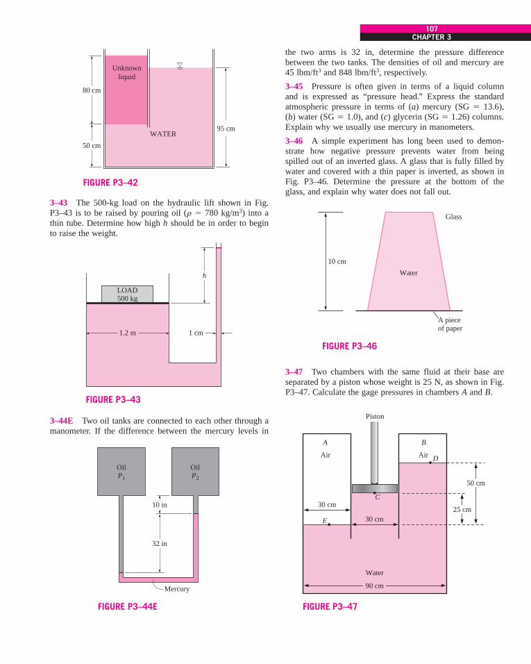
CHAPTER 3107

3–43 The 500-kg load on the hydraulic lift shown in Fig.P3–43 is to be raised by pouring oil (r " 780 kg/m3) into athin tube. Determine how high h should be in order to beginto raise the weight.

the two arms is 32 in, determine the pressure differencebetween the two tanks. The densities of oil and mercury are45 lbm/ft3 and 848 lbm/ft3, respectively.

3–45 Pressure is often given in terms of a liquid columnand is expressed as “pressure head.” Express the standardatmospheric pressure in terms of (a) mercury (SG " 13.6),(b) water (SG " 1.0), and (c) glycerin (SG " 1.26) columns.Explain why we usually use mercury in manometers.

3–46 A simple experiment has long been used to demon-strate how negative pressure prevents water from beingspilled out of an inverted glass. A glass that is fully filled bywater and covered with a thin paper is inverted, as shown inFig. P3–46. Determine the pressure at the bottom of theglass, and explain why water does not fall out.

50 cm

95 cm

80 cm

Unknownliquid

WATER

FIGURE P3–42

LOAD500 kg

h

1.2 m 1 cm

FIGURE P3–43

3–44E Two oil tanks are connected to each other through amanometer. If the difference between the mercury levels in

OilP1

OilP2

10 in

32 in

Mercury

FIGURE P3–44E

Glass

Water

A pieceof paper

10 cm

FIGURE P3–46

3–47 Two chambers with the same fluid at their base areseparated by a piston whose weight is 25 N, as shown in Fig.P3–47. Calculate the gage pressures in chambers A and B.

Water

Air

E

C

Air

A B

Piston

50 cm

25 cm30 cm

30 cm

90 cm

D

FIGURE P3–47

cen72367_ch03.qxd 10/29/04 2:22 PM Page 107

3–48 Consider a double-fluid manometer attached to an airpipe shown in Fig. P3–48. If the specific gravity of one fluidis 13.55, determine the specific gravity of the other fluid forthe indicated absolute pressure of air. Take the atmosphericpressure to be 100 kPa. Answer: 5.0

108FLUID MECHANICS

3–51 Two water tanks are connected to each other througha mercury manometer with inclined tubes, as shown in Fig.P3–51. If the pressure difference between the two tanks is20 kPa, calculate a and u.

SG2

Air

P = 76 kPa

22 cm

40 cm

SG1 = 13.55

FIGURE P3–48

3–49 The pressure difference between an oil pipe and waterpipe is measured by a double-fluid manometer, as shown inFig. P3–49. For the given fluid heights and specific gravities,calculate the pressure difference $P " PB # PA.

OilSG = 0.88

GlycerinSG = 1.26Water

SG = 1.0

MercurySG = 13.5

A

B

20 cm

60 cm

10 cm

15 cm

FIGURE P3–49

3–50 Consider the system shown in Fig. P3–50. If a changeof 0.7 kPa in the pressure of air causes the brine-mercuryinterface in the right column to drop by 5 mm in the brinelevel in the right column while the pressure in the brine piperemains constant, determine the ratio of A2/A1.

MercurySG = 13.56

Water

Air

Area, A1

Area, A2

Brine pipe

SG = 1.1

FIGURE P3–50

Water A

MercurySG = 13.6

2a

u

26.8 cma

a

Water B

FIGURE P3–51

3–52 A multifluid container is connected to a U-tube, asshown in Fig. P3–52. For the given specific gravities andfluid column heights, determine the gage pressure at A. Alsodetermine the height of a mercury column that would createthe same pressure at A. Answers: 0.471 kPa, 0.353 cm

cen72367_ch03.qxd 10/29/04 2:22 PM Page 108

CHAPTER 3109

Fluid Statics: Hydrostatic Forces on Plane and Curved Surfaces3–53C Define the resultant hydrostatic force acting on asubmerged surface, and the center of pressure.

3–54C Someone claims that she can determine the magni-tude of the hydrostatic force acting on a plane surface sub-merged in water regardless of its shape and orientation if sheknew the vertical distance of the centroid of the surface fromthe free surface and the area of the surface. Is this a validclaim? Explain.

3–55C A submerged horizontal flat plate is suspended inwater by a string attached at the centroid of its upper surface.Now the plate is rotated 45° about an axis that passes throughits centroid. Discuss the change on the hydrostatic force act-ing on the top surface of this plate as a result of this rotation.Assume the plate remains submerged at all times.

3–56C You may have noticed that dams are much thicker atthe bottom. Explain why dams are built that way.

3–57C Consider a submerged curved surface. Explain howyou would determine the horizontal component of the hydro-static force acting on this surface.

3–58C Consider a submerged curved surface. Explain howyou would determine the vertical component of the hydrosta-tic force acting on this surface.

3–59C Consider a circular surface subjected to hydrostaticforces by a constant density liquid. If the magnitudes of thehorizontal and vertical components of the resultant hydrosta-tic force are determined, explain how you would find the lineof action of this force.

3–60 Consider a heavy car submerged in water in a lakewith a flat bottom. The driver’s side door of the car is 1.1 mhigh and 0.9 m wide, and the top edge of the door is 8 mbelow the water surface. Determine the net force acting onthe door (normal to its surface) and the location of the pres-

sure center if (a) the car is well-sealed and it contains air atatmospheric pressure and (b) the car is filled with water.

3–61E A long, solid cylinder of radius 2 ft hinged at pointA is used as an automatic gate, as shown in Fig. P3–61E.When the water level reaches 15 ft, the cylindrical gate opensby turning about the hinge at point A. Determine (a) thehydrostatic force acting on the cylinder and its line of actionwhen the gate opens and (b) the weight of the cylinder per ftlength of the cylinder.

70 cmOil

SG = 0.90

Water

GlycerinSG = 1.26

30 cm

20 cm

15 cm

90 cm

A

FIGURE P3–52A

15 ft

2 ft

FIGURE P3–61E

Sea5 m

30 cm

FIGURE P3–64

3–62 Consider a 4-m-long, 4-m-wide, and 1.5-m-highaboveground swimming pool that is filled with water to therim. (a) Determine the hydrostatic force on each wall and thedistance of the line of action of this force from the ground.(b) If the height of the walls of the pool is doubled and thepool is filled, will the hydrostatic force on each wall doubleor quadruple? Why? Answer: (a) 44.1 kN

3–63E Consider a 200-ft-high, 1200-ft-wide dam filled tocapacity. Determine (a) the hydrostatic force on the dam and(b) the force per unit area of the dam near the top and nearthe bottom.

3–64 A room in the lower level of a cruise ship has a 30-cm-diameter circular window. If the midpoint of the win-dow is 5 m below the water surface, determine the hydro-static force acting on the window, and the pressure center.Take the specific gravity of seawater to be 1.025. Answers:3554 N, 5.001 m

cen72367_ch03.qxd 10/29/04 2:22 PM Page 109

3–72 Repeat Prob. 3–71 for the case of a partially filledtrough with a water height of 0.4 m directly above the hinge.

3–73 A retaining wall against a mud slide is to be con-structed by placing 0.8-m-high and 0.2-m-wide rectangularconcrete blocks (r " 2700 kg/m3) side by side, as shown inFig. P3–73. The friction coefficient between the ground andthe concrete blocks is f " 0.3, and the density of the mud isabout 1800 kg/m3. There is concern that the concrete blocksmay slide or tip over the lower left edge as the mud levelrises. Determine the mud height at which (a) the blocks will

3–65 The water side of the wall of a 100-m-long dam is aquarter circle with a radius of 10 m. Determine the hydro-static force on the dam and its line of action when the dam isfilled to the rim.

3–66 A 4-m-high, 5-m-wide rectangular plate blocks theend of a 4-m-deep freshwater channel, as shown in Fig.P3–66. The plate is hinged about a horizontal axis along itsupper edge through a point A and is restrained from openingby a fixed ridge at point B. Determine the force exerted onthe plate by the ridge.

110FLUID MECHANICS

3–69E Repeat Prob. 3–68E for a water height of 8 ft.

3–70 A water trough of semicircular cross section of radius0.5 m consists of two symmetric parts hinged to each other atthe bottom, as shown in Fig. P3–70. The two parts are held

3–67 Reconsider Prob. 3–66. Using EES (or other)software, investigate the effect of water depth on

the force exerted on the plate by the ridge. Let the waterdepth vary from 0 m to 5 m in increments of 0.5 m. Tabulateand plot your results.

3–68E The flow of water from a reservoir is controlled by a5-ft-wide L-shaped gate hinged at point A, as shown in Fig.P3–68E. If it is desired that the gate open when the waterheight is 12 ft, determine the mass of the required weight W.Answer: 30,900 lbm

1 m

4 m

A

B

FIGURE P3–66

together by a cable and turnbuckle placed every 3 m alongthe length of the trough. Calculate the tension in each cablewhen the trough is filled to the rim.

AB

5 ft

12 ft15 ftGate

W

FIGURE P3–68E

3–71 The two sides of a V-shaped water trough are hingedto each other at the bottom where they meet, as shown in Fig.P3–71, making an angle of 45° with the ground from bothsides. Each side is 0.75 m wide, and the two parts are heldtogether by a cable and turnbuckle placed every 6 m alongthe length of the trough. Calculate the tension in each cablewhen the trough is filled to the rim. Answer: 5510 N

1 mCable

Hinge

FIGURE P3–70

0.75 m45° 45°

Cable

Hinge

FIGURE P3–71

0.8 m Mudrm

h

0.2 m

FIGURE P3–73

cen72367_ch03.qxd 10/29/04 2:22 PM Page 110

CHAPTER 3111

3–83E A crane is used to lower weights into a lake for anunderwater construction project. Determine the tension in therope of the crane due to a 3-ft-diameter spherical steel block(density " 494 lbm/ft3) when it is (a) suspended in the airand (b) completely immersed in water.

3–84 The volume and the average density of an irregularlyshaped body are to be determined by using a spring scale.The body weighs 7200 N in air and 4790 N in water. Deter-mine the volume and the density of the body. State yourassumptions.

3–85 Consider a large cubic ice block floating in seawater.The specific gravities of ice and seawater are 0.92 and 1.025,respectively. If a 10-cm-high portion of the ice block extendsabove the surface of the water, determine the height of the iceblock below the surface. Answer: 87.6 cm

overcome friction and start sliding and (b) the blocks will tipover.

3–74 Repeat Prob. 3–73 for 0.4-m-wide concrete blocks.

3–75 A 4-m-long quarter-circular gate of radius 3 mand of negligible weight is hinged about its

upper edge A, as shown in Fig. P3–75. The gate controls theflow of water over the ledge at B, where the gate is pressedby a spring. Determine the minimum spring force required tokeep the gate closed when the water level rises to A at theupper edge of the gate.

3–76 Repeat Prob. 3–75 for a radius of 4 m for the gate.Answer: 314 kN

Buoyancy3–77C What is buoyant force? What causes it? What is themagnitude of the buoyant force acting on a submerged bodywhose volume is V? What are the direction and the line ofaction of the buoyant force?

3–78C Consider two identical spherical balls submerged inwater at different depths. Will the buoyant forces acting onthese two balls be the same or different? Explain.

3–79C Consider two 5-cm-diameter spherical balls—onemade of aluminum, the other of iron—submerged in water.Will the buoyant forces acting on these two balls be the sameor different? Explain.

3–80C Consider a 3-kg copper cube and a 3-kg copper ballsubmerged in a liquid. Will the buoyant forces acting onthese two bodies be the same or different? Explain.

3–81C Discuss the stability of (a) a submerged and (b) afloating body whose center of gravity is above the center ofbuoyancy.

3–82 The density of a liquid is to be determined by an old1-cm-diameter cylindrical hydrometer whose division marksare completely wiped out. The hydrometer is first dropped inwater, and the water level is marked. The hydrometer is thendropped into the other liquid, and it is observed that the markfor water has risen 0.5 cm above the liquid–air interface. Ifthe height of the water mark is 10 cm, determine the densityof the liquid.

A

B

3 m

Spring

FIGURE P3–75

3–86 A 170-kg granite rock (r " 2700 kg/m3) is droppedinto a lake. A man dives in and tries to lift the rock. Deter-mine how much force the man needs to apply to lift it fromthe bottom of the lake. Do you think he can do it?

3–87 It is said that Archimedes discovered his principleduring a bath while thinking about how he could determine ifKing Hiero’s crown was actually made of pure gold. While inthe bathtub, he conceived the idea that he could determine

Mark forwater

Unknownliquid

0.5 cm

10 cm

FIGURE P3–82

Sea

10 cm

Cubicice block h

FIGURE P3–85

cen72367_ch03.qxd 10/29/04 2:22 PM Page 111

the average density of an irregularly shaped object by weigh-ing it in air and also in water. If the crown weighed 3.20 kgf(" 31.4 N) in air and 2.95 kgf (" 28.9 N) in water, deter-mine if the crown is made of pure gold. The density of goldis 19,300 kg/m3. Discuss how you can solve this problemwithout weighing the crown in water but by using an ordi-nary bucket with no calibration for volume. You may weighanything in air.

3–88 One of the common procedures in fitness programs isto determine the fat-to-muscle ratio of the body. This is basedon the principle that the muscle tissue is denser than the fattissue, and, thus, the higher the average density of the body,the higher is the fraction of muscle tissue. The average densityof the body can be determined by weighing the person in airand also while submerged in water in a tank. Treating all tis-sues and bones (other than fat) as muscle with an equivalentdensity of rmuscle, obtain a relation for the volume fraction ofbody fat xfat. Answer: xfat " (rmuscle # rave)/(rmuscle # rfat).

112FLUID MECHANICS

3–93C Consider a vertical cylindrical container partiallyfilled with water. Now the cylinder is rotated about its axis ata specified angular velocity, and rigid-body motion is estab-lished. Discuss how the pressure will be affected at the mid-point and at the edges of the bottom surface due to rotation.

3–94 A water tank is being towed by a truck on a levelroad, and the angle the free surface makes with the horizontalis measured to be 15°. Determine the acceleration of thetruck.

3–95 Consider two water tanks filled with water. The firsttank is 8 m high and is stationary, while the second tank is 2m high and is moving upward with an acceleration of 5 m/s2.Which tank will have a higher pressure at the bottom?

3–96 A water tank is being towed on an uphill road thatmakes 20° with the horizontal with a constant acceleration of5 m/s2 in the direction of motion. Determine the angle thefree surface of water makes with the horizontal. What wouldyour answer be if the direction of motion were downward onthe same road with the same acceleration?

3–97E A 2-ft-diameter vertical cylindrical tank open to theatmosphere contains 1-ft-high water. The tank is now rotatedabout the centerline, and the water level drops at the centerwhile it rises at the edges. Determine the angular velocity atwhich the bottom of the tank will first be exposed. Alsodetermine the maximum water height at this moment.

3–89 The hull of a boat has a volume of 150 m3, and thetotal mass of the boat when empty is 8560 kg. Determinehow much load this boat can carry without sinking (a) in alake and (b) in seawater with a specific gravity of 1.03.

Fluids in Rigid-Body Motion3–90C Under what conditions can a moving body of fluidbe treated as a rigid body?

3–91C Consider a glass of water. Compare the water pres-sures at the bottom surface for the following cases: the glassis (a) stationary, (b) moving up at constant velocity, (c) mov-ing down at constant velocity, and (d) moving horizontally atconstant velocity.

3–92C Consider two identical glasses of water, one station-ary and the other moving on a horizontal plane with constantacceleration. Assuming no splashing or spilling occurs, whichglass will have a higher pressure at the (a) front, (b) mid-point, and (c) back of the bottom surface?

Submergedperson

Water tank

Springscale

FIGURE P3–88E

3–98 A 60-cm-high, 40-cm-diameter cylindrical water tankis being transported on a level road. The highest accelerationanticipated is 4 m/s2. Determine the allowable initial waterheight in the tank if no water is to spill out during accelera-tion. Answer: 51.8 cm

3–99 A 40-cm-diameter, 90-cm-high vertical cylindricalcontainer is partially filled with 60-cm-high water. Now thecylinder is rotated at a constant angular speed of 120 rpm.Determine how much the liquid level at the center of thecylinder will drop as a result of this rotational motion.

3–100 A fish tank that contains 40-cm-high water is movedin the cabin of an elevator. Determine the pressure at the bot-

2 ft

&

FIGURE P3–97E

cen72367_ch03.qxd 10/29/04 2:22 PM Page 112

CHAPTER 3113

tom of the tank when the elevator is (a) stationary, (b) mov-ing up with an upward acceleration of 3 m/s2, and (c) movingdown with a downward acceleration of 3 m/s2.

3–101 A 3-m-diameter vertical cylindrical milk tank rotatesat a constant rate of 12 rpm. If the pressure at the center ofthe bottom surface is 130 kPa, determine the pressure at theedge of the bottom surface of the tank. Take the density ofthe milk to be 1030 kg/m.

3–102 Milk with a density of 1020 kg/m3 is transported ona level road in a 7-m-long, 3-m-diameter cylindrical tanker.The tanker is completely filled with milk (no air space), andit accelerates at 2.5 m/s2. If the minimum pressure in thetanker is 100 kPa, determine the maximum pressure and itslocation. Answer: 47.9 kPa

at the centers of the bottom and top surfaces and (b) the dif-ference between the pressures at the center and the edge ofthe bottom surface.

3–103 Repeat Prob. 3–102 for a deceleration of 2.5 m/s2.

3–104 The distance between the centers of the two arms ofa U-tube open to the atmosphere is 25 cm, and the U-tubecontains 20-cm-high alcohol in both arms. Now the U-tube isrotated about the left arm at 4.2 rad/s. Determine the eleva-tion difference between the fluid surfaces in the two arms.

7 m

3 m

FIGURE P3–102

3–106 Reconsider Prob. 3–105. Using EES (or other)software, investigate the effect of rotational

speed on the pressure difference between the center and theedge of the bottom surface of the cylinder. Let the rotationalspeed vary from 0 rpm to 500 rpm in increments of 50 rpm.Tabulate and plot your results.

3–107E A 20-ft-long, 8-ft-high rectangular tank open to theatmosphere is towed by a truck on a level road. The tank isfilled with water to a depth of 6 ft. Determine the maximumacceleration or deceleration allowed if no water is to spillduring towing.

3–108E An 8-ft-long tank open to the atmosphere initiallycontains 3-ft-high water. It is being towed by a truck on alevel road. The truck driver applies the brakes and the waterlevel at the front rises 0.5 ft above the initial level. Determinethe deceleration of the truck. Answer: 4.08 ft/s2

25 cm

20 cm

FIGURE P3–104

3–105 A 1.2-m-diameter, 3-m-high sealed vertical cylinderis completely filled with gasoline whose density is 740 kg/m3.The tank is now rotated about its vertical axis at a rate of70 rpm. Determine (a) the difference between the pressures

3 m1.20 m

FIGURE P3–105

8 ft

Water3 ft

0.5 ft

FIGURE P3–108E

cen72367_ch03.qxd 10/29/04 2:22 PM Page 113

3–109 A 3-m-diameter, 7-m-long cylindrical tank is com-pletely filled with water. The tank is pulled by a truck on alevel road with the 7-m-long axis being horizontal. Deter-mine the pressure difference between the front and back endsof the tank along a horizontal line when the truck (a) acceler-ates at 3 m/s2 and (b) decelerates at 4 m/s2.

Review Problems3–110 An air-conditioning system requires a 20-m-longsection of 15-cm-diameter ductwork to be laid underwater.Determine the upward force the water will exert on the duct.Take the densities of air and water to be 1.3 kg/m3 and 1000kg/m3, respectively.

3–111 Balloons are often filled with helium gas because itweighs only about one-seventh of what air weighs underidentical conditions. The buoyancy force, which can beexpressed as Fb " rairgVballoon, will push the balloon upward.If the balloon has a diameter of 10 m and carries two people,70 kg each, determine the acceleration of the balloon when itis first released. Assume the density of air is r " 1.16 kg/m3,and neglect the weight of the ropes and the cage. Answer:16.5 m/s2

114FLUID MECHANICS

3–115 The basic barometer can be used as an altitude-measuring device in airplanes. The ground control reports abarometric reading of 753 mmHg while the pilot’s reading is690 mmHg. Estimate the altitude of the plane from groundlevel if the average air density is 1.20 kg/m3. Answer: 714 m

3–116 The lower half of a 10-m-high cylindrical containeris filled with water (r " 1000 kg/m3) and the upper half withoil that has a specific gravity of 0.85. Determine the pressuredifference between the top and bottom of the cylinder.Answer: 90.7 kPa

3–112 Reconsider Prob. 3–111. Using EES (or other)software, investigate the effect of the number

of people carried in the balloon on acceleration. Plot theacceleration against the number of people, and discuss theresults.

3–113 Determine the maximum amount of load, in kg, theballoon described in Prob. 3–111 can carry. Answer:520.6 kg

3–114E The pressure in a steam boiler is given to be 75kgf/cm2. Express this pressure in psi, kPa, atm, and bars.

HELIUMD = 10 mrHe = rair

17

m = 140 kg

FIGURE P3–111

3–117 A vertical, frictionless piston–cylinder device con-tains a gas at 500 kPa. The atmospheric pressure outside is100 kPa, and the piston area is 30 cm2. Determine the massof the piston.

3–118 A pressure cooker cooks a lot faster than an ordinarypan by maintaining a higher pressure and temperature inside.The lid of a pressure cooker is well sealed, and steam canescape only through an opening in the middle of the lid. Aseparate metal piece, the petcock, sits on top of this opening

OIL

SG = 0.85

h = 10 m

' = 1000 kg/m3WATER

FIGURE P3–116

Patm = 101 kPa

Petcock

PRESSURECOOKER

A = 4 mm2

FIGURE P3–118

cen72367_ch03.qxd 10/29/04 2:22 PM Page 114

CHAPTER 3115

and prevents steam from escaping until the pressure forceovercomes the weight of the petcock. The periodic escape ofthe steam in this manner prevents any potentially dangerouspressure buildup and keeps the pressure inside at a constantvalue. Determine the mass of the petcock of a pressurecooker whose operation pressure is 100 kPa gage and has anopening cross-sectional area of 4 mm2. Assume an atmos-pheric pressure of 101 kPa, and draw the free-body diagramof the petcock. Answer: 40.8 g

3–119 A glass tube is attached to a water pipe, as shown inFig. P3–119. If the water pressure at the bottom of the tube is115 kPa and the local atmospheric pressure is 92 kPa, deter-mine how high the water will rise in the tube, in m. Assumeg " 9.8 m/s2 at that location and take the density of water tobe 1000 kg/m3.

cular duct is to be measured using a manometer whose openarm is inclined 35° from the horizontal, as shown in Fig.P3–121. The density of the liquid in the manometer is 0.81kg/L, and the vertical distance between the fluid levels in thetwo arms of the manometer is 8 cm. Determine the gagepressure of air in the duct and the length of the fluid columnin the inclined arm above the fluid level in the vertical arm.

3–122E Consider a U-tube whose arms are open to theatmosphere. Now equal volumes of water and light oil (r" 49.3 lbm/ft3) are poured from different arms. A personblows from the oil side of the U-tube until the contact surfaceof the two fluids moves to the bottom of the U-tube, and thus

3–120 The average atmospheric pressure on earth isapproximated as a function of altitude by the relation Patm" 101.325 (1 # 0.02256z)5.256, where Patm is the atmosphericpressure in kPa and z is the altitude in km with z " 0 at sealevel. Determine the approximate atmospheric pressures atAtlanta (z " 306 m), Denver (z " 1610 m), Mexico City (z" 2309 m), and the top of Mount Everest (z " 8848 m).

3–121 When measuring small pressure differences with amanometer, often one arm of the manometer is inclined toimprove the accuracy of reading. (The pressure difference isstill proportional to the vertical distance and not the actuallength of the fluid along the tube.) The air pressure in a cir-

Patm = 92 kPa

h = ?

Water

FIGURE P3–119

the liquid levels in the two arms are the same. If the fluidheight in each arm is 30 in, determine the gage pressure theperson exerts on the oil by blowing.

3–123 Intravenous infusions are usually driven by gravityby hanging the fluid bottle at sufficient height to counteractthe blood pressure in the vein and to force the fluid into thebody. The higher the bottle is raised, the higher the flow rateof the fluid will be. (a) If it is observed that the fluid and theblood pressures balance each other when the bottle is 1.2 mabove the arm level, determine the gage pressure of theblood. (b) If the gage pressure of the fluid at the arm levelneeds to be 20 kPa for sufficient flow rate, determine howhigh the bottle must be placed. Take the density of the fluidto be 1020 kg/m3.

Duct

35°

8 cmL

Air

FIGURE P3–121

Air

Water 30 inOil

FIGURE P3–122E

1.2 m

Patm

IV bottle

FIGURE P3–123

cen72367_ch03.qxd 10/29/04 2:22 PM Page 115

3–124 A gasoline line is connected to a pressure gagethrough a double-U manometer, as shown in Fig. P3–124. Ifthe reading of the pressure gage is 370 kPa, determine thegage pressure of the gasoline line.

116FLUID MECHANICS

3–125 Repeat Prob. 3–124 for a pressure gage reading of240 kPa.

3–126E A water pipe is connected to a double-U manome-ter as shown in Fig. P3–1026E at a location where the localatmospheric pressure is 14.2 psia. Determine the absolutepressure at the center of the pipe.

3–127 The pressure of water flowing through a pipe is mea-sured by the arrangement shown in Fig. P3–127. For the val-ues given, calculate the pressure in the pipe.

45 cm

10 cm

22 cm50 cm

MercurySG = 13.6

Gasoline SG = 0.70

Water

Air

Oil SG = 0.79Pgage = 370 kPa

Pipe

FIGURE P3–124

3–128 Consider a U-tube filled with mercury except the 18-cm-high portion at the top, as shown in Fig. P3–128. Thediameter of the right arm of the U-tube is D " 2 cm, and thediameter of the left arm is twice that. Oil with a specificgravity of 2.72 is poured into the left arm, forcing some mer-cury from the left arm into the right one. Determine the max-imum amount of oil that can be added into the left arm.Answer: 0.256 L

MercurySG = 13.6

Oil SG = 0.80

Oil SG = 0.80

Waterpipe

15 in

40 in60 in

35 in

FIGURE P3–126E

Water15°C

Air

P0 = 30 kPa

u

Gage fluidSG = 2.4

Water

Pipe

h1 = 8 cmL1 = 6 cm

L2 = 6 cm

h2 = 50 cm15°C

FIGURE P3–127

OilSG = 2.72

D = 2 cm2D

18 cm

MercurySG = 13.6

FIGURE P3–128

cen72367_ch03.qxd 10/29/04 2:22 PM Page 116

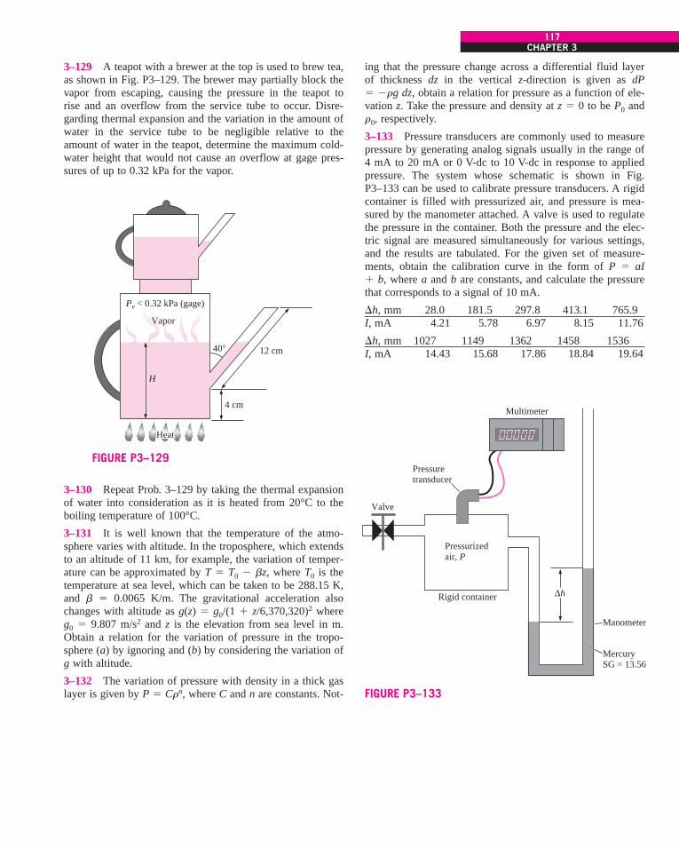
CHAPTER 3117

3–130 Repeat Prob. 3–129 by taking the thermal expansionof water into consideration as it is heated from 20°C to theboiling temperature of 100°C.

3–131 It is well known that the temperature of the atmo-sphere varies with altitude. In the troposphere, which extendsto an altitude of 11 km, for example, the variation of temper-ature can be approximated by T " T0 # bz, where T0 is thetemperature at sea level, which can be taken to be 288.15 K,and b " 0.0065 K/m. The gravitational acceleration alsochanges with altitude as g(z) " g0/(1 ! z/6,370,320)2 whereg0 " 9.807 m/s2 and z is the elevation from sea level in m.Obtain a relation for the variation of pressure in the tropo-sphere (a) by ignoring and (b) by considering the variation ofg with altitude.

3–132 The variation of pressure with density in a thick gaslayer is given by P " Crn, where C and n are constants. Not-

ing that the pressure change across a differential fluid layerof thickness dz in the vertical z-direction is given as dP" #rg dz, obtain a relation for pressure as a function of ele-vation z. Take the pressure and density at z " 0 to be P0 andr0, respectively.

3–133 Pressure transducers are commonly used to measurepressure by generating analog signals usually in the range of4 mA to 20 mA or 0 V-dc to 10 V-dc in response to appliedpressure. The system whose schematic is shown in Fig.P3–133 can be used to calibrate pressure transducers. A rigidcontainer is filled with pressurized air, and pressure is mea-sured by the manometer attached. A valve is used to regulatethe pressure in the container. Both the pressure and the elec-tric signal are measured simultaneously for various settings,and the results are tabulated. For the given set of measure-ments, obtain the calibration curve in the form of P " aI! b, where a and b are constants, and calculate the pressurethat corresponds to a signal of 10 mA.

$h, mm 28.0 181.5 297.8 413.1 765.9I, mA 4.21 5.78 6.97 8.15 11.76

$h, mm 1027 1149 1362 1458 1536I, mA 14.43 15.68 17.86 18.84 19.64

3–129 A teapot with a brewer at the top is used to brew tea,as shown in Fig. P3–129. The brewer may partially block thevapor from escaping, causing the pressure in the teapot torise and an overflow from the service tube to occur. Disre-garding thermal expansion and the variation in the amount ofwater in the service tube to be negligible relative to theamount of water in the teapot, determine the maximum cold-water height that would not cause an overflow at gage pres-sures of up to 0.32 kPa for the vapor.

40° 12 cm

4 cm

H

Vapor

HeatHeat

Pv < 0.32 kPa (gage)

FIGURE P3–129Pressuretransducer

Valve

Pressurized air, P

Multimeter

Rigid container

Manometer

MercurySG = 13.56

%h

FIGURE P3–133

cen72367_ch03.qxd 10/29/04 2:22 PM Page 117

3–140 Repeat Prob. 3–139 for a total water height of 2 m.

3–141E A semicircular 30-ft-diameter tunnel is to be builtunder a 150-ft-deep, 800-ft-long lake, as shown in Fig.P3–141E. Determine the total hydrostatic force acting on theroof of the tunnel.

3–134 A system is equipped with two pressure gages and amanometer, as shown in Fig. P3–134. For $h " 8 cm, deter-mine the pressure difference $P " P2 # P1.

118FLUID MECHANICS

3–135 An oil pipeline and a 1.3-m3 rigid air tank are con-nected to each other by a manometer, as shown in Fig.P3–135. If the tank contains 15 kg of air at 80°C, determine(a) the absolute pressure in the pipeline and (b) the change in$h when the temperature in the tank drops to 20°C. Assumethe pressure in the oil pipeline to remain constant, and the airvolume in the manometer to be negligible relative to the vol-ume of the tank.

Air

Manometerfluid SG = 2.67

%h%h

P1 P2

OilSG = 0.87

FIGURE P3–134

1.3 m3

Air, 80°COilSG = 2.68

h = 75 cm

D = 4 mmMercurySG = 13.6

50°

3D

%h = 20 cm

FIGURE P3–135

45°

B

A

0.5 m

3 m

Water

F

FIGURE P3–137

2 m

Water

Gate3 m

A

B

FIGURE P3–139

3–138 Repeat Prob. 3–137 for a water height of 1.2 mabove the hinge at B.

3–139 A 3-m-high, 6-m-wide rectangular gate is hinged atthe top edge at A and is restrained by a fixed ridge at B.Determine the hydrostatic force exerted on the gate by the5-m-high water and the location of the pressure center.

3–136 The density of a floating body can be determined bytying weights to the body until both the body and the weightsare completely submerged, and then weighing them sepa-

rately in air. Consider a wood log that weighs 1540 N in air.If it takes 34 kg of lead (r " 11,300 kg/m3) to completelysink the log and the lead in water, determine the average den-sity of the log. Answer: 835 kg/m3

3–137 The 200-kg, 5-m-wide rectangular gate shownin Fig. P3–137 is hinged at B and leans against

the floor at A making an angle of 45° with the horizontal.The gate is to be opened from its lower edge by applying anormal force at its center. Determine the minimum force Frequired to open the water gate. Answer: 520 kN

cen72367_ch03.qxd 10/29/04 2:22 PM Page 118

CHAPTER 3119

3–143 The water in a 25-m-deep reservoir is kept inside bya 150-m-wide wall whose cross section is an equilateral tri-angle, as shown in Fig. P3–143. Determine (a) the total force(hydrostatic ! atmospheric) acting on the inner surface ofthe wall and its line of action and (b) the magnitude of thehorizontal component of this force. Take Patm " 100 kPa.

3–142 A 50-ton, 6-m-diameter hemispherical dome on alevel surface is filled with water, as shown in Fig. P3–142.Someone claims that he can lift this dome by making use ofPascal’s law by attaching a long tube to the top and filling itwith water. Determine the required height of water in thetube to lift the dome. Disregard the weight of the tube andthe water in it. Answer: 0.77 m

3–144 A U-tube contains water in the right arm, andanother liquid in the left arm. It is observed that when the U-tube rotates at 30 rpm about an axis that is 15 cm from theright arm and 5 cm from the left arm, the liquid levels in botharms become the same. Determine the density of the fluid inthe left arm.

Water

150 ft

30 ft

Tunnel

FIGURE P3–141E

50 ton

h

6 m

Water

FIGURE P3–142

Water

60° 60°

25 m

FIGURE P3–143

15 cm5 cm

10 cm

FIGURE P3–144

3–145 A 1-m-diameter, 2-m-high vertical cylinder is com-pletely filled with gasoline whose density is 740 kg/m3. Thetank is now rotated about its vertical axis at a rate of 90 rpm,while being accelerated upward at 5 m/s2. Determine (a) thedifference between the pressures at the centers of the bottomand top surfaces and (b) the difference between the pressuresat the center and the edge of the bottom surface.

2 m

5 m/s2

1 m

FIGURE P3–145

3–146 A 5-m-long, 4-m-high tank contains 2.5-m-deepwater when not in motion and is open to the atmospherethrough a vent in the middle. The tank is now accelerated to

cen72367_ch03.qxd 10/29/04 2:22 PM Page 119

the right on a level surface at 2 m/s2. Determine the maxi-mum pressure in the tank relative to the atmospheric pres-sure. Answer: 29.5 kPa

120FLUID MECHANICS

3–149 Reconsider Prob. 3–148. Using EES (or other)software, investigate the effect of air pressure

above water on the cable force. Let this pressure vary from 0.1MPa to 10 MPa. Plot the cable force versus the air pressure.

3–150 The average density of icebergs is about 917 kg/m3.(a) Determine the percentage of the total volume of an ice-berg submerged in seawater of density 1042 kg/m3. (b)Although icebergs are mostly submerged, they are observedto turn over. Explain how this can happen. (Hint: Considerthe temperatures of icebergs and seawater.)

3–151 A cylindrical container whose weight is 79 N isinverted and pressed into the water, as shown in Fig. P3–151.Determine the differential height h of the manometer and theforce F needed to hold the container at the position shown.

3–147 Reconsider Prob. 3–146. Using EES (or other)software, investigate the effect of acceleration

on the slope of the free surface of water in the tank. Let theacceleration vary from 0 m/s2 to 5 m/s2 in increments of 0.5m/s2. Tabulate and plot your results.

3–148 An elastic air balloon having a diameter of 30 cm isattached to the base of a container partially filled with waterat !4°C, as shown in Fig. P3–148. If the pressure of airabove water is gradually increased from 100 kPa to 1.6 MPa,will the force on the cable change? If so, what is the percentchange in the force? Assume the pressure on the free surfaceand the diameter of the balloon are related by P " CDn,where C is a constant and n " #2. The weight of the balloonand the air in it is negligible. Answer: 98.4 percent

Design and Essay Problems3–152 Shoes are to be designed to enable people of up to80 kg to walk on freshwater or seawater. The shoes are to bemade of blown plastic in the shape of a sphere, a (American)football, or a loaf of French bread. Determine the equivalentdiameter of each shoe and comment on the proposed shapesfrom the stability point of view. What is your assessment ofthe marketability of these shoes?

3–153 The volume of a rock is to be determined withoutusing any volume measurement devices. Explain how youwould do this with a waterproof spring scale.

5 m

Vent

Watertank2.5 m

1.5 m

2 m/s2

FIGURE P3–146

50 cm

Water

50 cm

20 cmP1 = 100 kPa

D1 = 30 cm

FIGURE P3–148

D = 30 cm

Manometer fluidSG = 2.1Air

20 cm Water

h

F

FIGURE P3–151

cen72367_ch03.qxd 10/29/04 2:22 PM Page 120

F L U I D K I N E M AT I C S

Fluid kinematics deals with describing the motion of fluids without nec-essarily considering the forces and moments that cause the motion. Inthis chapter, we introduce several kinematic concepts related to flow-

ing fluids. We discuss the material derivative and its role in transformingthe conservation equations from the Lagrangian description of fluid flow(following a fluid particle) to the Eulerian description of fluid flow (pertain-ing to a flow field). We then discuss various ways to visualize flow fields—streamlines, streaklines, pathlines, timelines, and optical methods schlierenand shadowgraph—and we describe three ways to plot flow data—profileplots, vector plots, and contour plots. We explain the four fundamental kine-matic properties of fluid motion and deformation—rate of translation, rateof rotation, linear strain rate, and shear strain rate. The concepts of vortic-ity, rotationality, and irrotationality in fluid flows are also discussed.Finally, we discuss the Reynolds transport theorem (RTT), emphasizing itsrole in transforming the equations of motion from those following a systemto those pertaining to fluid flow into and out of a control volume. The anal-ogy between material derivative for infinitesimal fluid elements and RTT forfinite control volumes is explained.

121

CHAPTER

4OBJECTIVESWhen you finish reading this chapter, youshould be able to

! Understand the role of thematerial derivative intransforming betweenLagrangian and Euleriandescriptions

! Distinguish between varioustypes of flow visualizations and methods of plotting thecharacteristics of a fluid flow

! Have an appreciation for themany ways that fluids move and deform

! Distinguish between rotationaland irrotational regions of flowbased on the flow propertyvorticity

! Understand the usefulness ofthe Reynolds transport theorem

cen72367_ch04.qxd 12/1/04 6:19 PM Page 121

4–1 ! LAGRANGIAN AND EULERIAN DESCRIPTIONSThe subject called kinematics concerns the study of motion. In fluiddynamics, fluid kinematics is the study of how fluids flow and how todescribe fluid motion. From a fundamental point of view, there are two dis-tinct ways to describe motion. The first and most familiar method is the oneyou learned in high school physics class—to follow the path of individualobjects. For example, we have all seen physics experiments in which a ballon a pool table or a puck on an air hockey table collides with another ball orpuck or with the wall (Fig. 4–1). Newton’s laws are used to describe themotion of such objects, and we can accurately predict where they go andhow momentum and kinetic energy are exchanged from one object to another.The kinematics of such experiments involves keeping track of the positionvector of each object, x

!

A, x!

B, . . . , and the velocity vector of each object,V!

A, V!

B, . . . , as functions of time (Fig. 4–2). When this method is applied toa flowing fluid, we call it the Lagrangian description of fluid motion afterthe Italian mathematician Joseph Louis Lagrange (1736–1813). Lagrangiananalysis is analogous to the system analysis that you learned in your ther-modynamics class; namely, we follow a mass of fixed identity

As you can imagine, this method of describing motion is much more dif-ficult for fluids than for billiard balls! First of all we cannot easily defineand identify particles of fluid as they move around. Secondly, a fluid is acontinuum (from a macroscopic point of view), so interactions betweenparcels of fluid are not as easy to describe as are interactions between dis-tinct objects like billiard balls or air hockey pucks. Furthermore, the fluidparcels continually deform as they move in the flow.

From a microscopic point of view, a fluid is composed of billions of mol-ecules that are continuously banging into one another, somewhat like bil-liard balls; but the task of following even a subset of these molecules isquite difficult, even for our fastest and largest computers. Nevertheless,there are many practical applications of the Lagrangian description, such asthe tracking of passive scalars in a flow, rarefied gas dynamics calculationsconcerning reentry of a spaceship into the earth’s atmosphere, and thedevelopment of flow measurement systems based on particle imaging (asdiscussed in Section 4–2).

A more common method of describing fluid flow is the Euleriandescription of fluid motion, named after the Swiss mathematician LeonhardEuler (1707–1783). In the Eulerian description of fluid flow, a finite volumecalled a flow domain or control volume is defined, through which fluidflows in and out. We do not need to keep track of the position and velocityof a mass of fluid particles of fixed identity. Instead, we define field vari-ables, functions of space and time, within the control volume. For example,the pressure field is a scalar field variable; for general unsteady three-dimensional fluid flow in Cartesian coordinates,

Pressure field: (4–1)

We define the velocity field as a vector field variable in similar fashion,

Velocity field: (4–2)

Likewise, the acceleration field is also a vector field variable,

Acceleration field: (4–3)a! ! a! (x, y, z, t)

V!

! V!

(x, y, z, t)

P ! P(x, y, z, t)

122FLUID MECHANICS

FIGURE 4–1With a small number of objects, suchas billiard balls on a pool table,individual objects can be tracked.

VB

VC

xA

xB xC

A

BC

VA!

!

!

!

!!

FIGURE 4–2In the Lagrangian description, onemust keep track of the position andvelocity of individual particles.

cen72367_ch04.qxd 12/1/04 6:19 PM Page 122

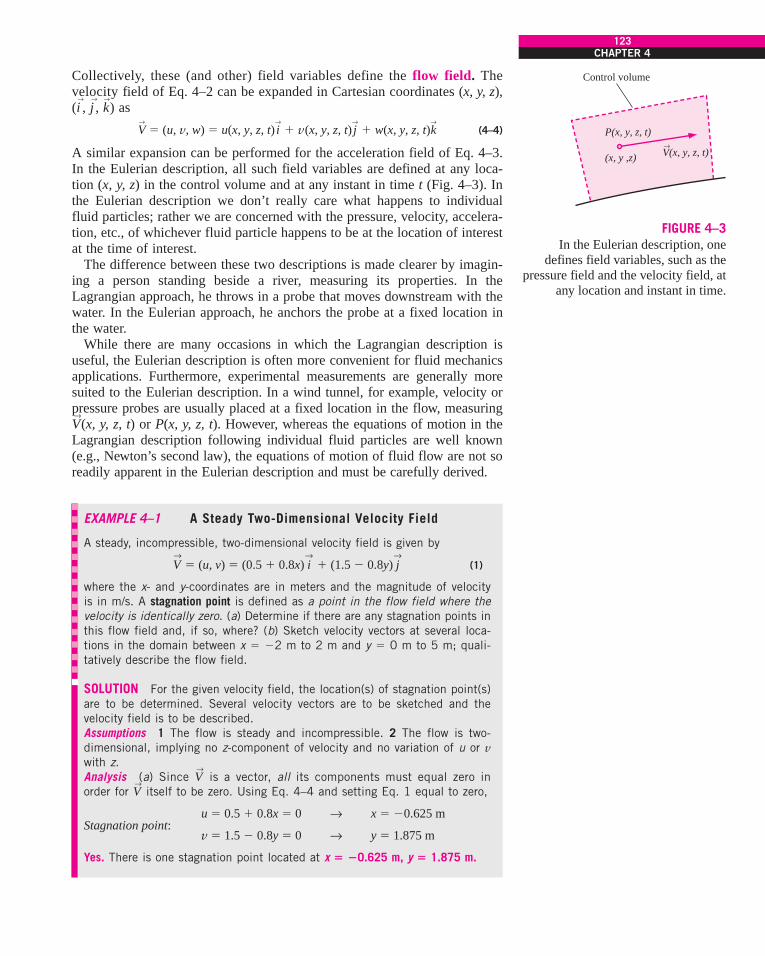
Collectively, these (and other) field variables define the flow field. Thevelocity field of Eq. 4–2 can be expanded in Cartesian coordinates (x, y, z),(i

!

, j!

, k!

) as

(4–4)

A similar expansion can be performed for the acceleration field of Eq. 4–3.In the Eulerian description, all such field variables are defined at any loca-tion (x, y, z) in the control volume and at any instant in time t (Fig. 4–3). Inthe Eulerian description we don’t really care what happens to individualfluid particles; rather we are concerned with the pressure, velocity, accelera-tion, etc., of whichever fluid particle happens to be at the location of interestat the time of interest.

The difference between these two descriptions is made clearer by imagin-ing a person standing beside a river, measuring its properties. In theLagrangian approach, he throws in a probe that moves downstream with thewater. In the Eulerian approach, he anchors the probe at a fixed location inthe water.

While there are many occasions in which the Lagrangian description isuseful, the Eulerian description is often more convenient for fluid mechanicsapplications. Furthermore, experimental measurements are generally moresuited to the Eulerian description. In a wind tunnel, for example, velocity orpressure probes are usually placed at a fixed location in the flow, measuringV!

(x, y, z, t) or P(x, y, z, t). However, whereas the equations of motion in theLagrangian description following individual fluid particles are well known(e.g., Newton’s second law), the equations of motion of fluid flow are not soreadily apparent in the Eulerian description and must be carefully derived.

EXAMPLE 4–1 A Steady Two-Dimensional Velocity Field

A steady, incompressible, two-dimensional velocity field is given by

(1)

where the x- and y-coordinates are in meters and the magnitude of velocityis in m/s. A stagnation point is defined as a point in the flow field where thevelocity is identically zero. (a) Determine if there are any stagnation points inthis flow field and, if so, where? (b) Sketch velocity vectors at several loca-tions in the domain between x ! "2 m to 2 m and y ! 0 m to 5 m; quali-tatively describe the flow field.

SOLUTION For the given velocity field, the location(s) of stagnation point(s)are to be determined. Several velocity vectors are to be sketched and thevelocity field is to be described.Assumptions 1 The flow is steady and incompressible. 2 The flow is two-dimensional, implying no z-component of velocity and no variation of u or vwith z.Analysis (a) Since V

!is a vector, all its components must equal zero in

order for V!

itself to be zero. Using Eq. 4–4 and setting Eq. 1 equal to zero,

Stagnation point:

Yes. There is one stagnation point located at x ! "0.625 m, y ! 1.875 m.

v ! 1.5 " 0.8y ! 0 ! y ! 1.875 m

u ! 0.5 # 0.8x ! 0 ! x ! "0.625 m

V!

! (u, v) ! (0.5 # 0.8x) i!

# (1.5 " 0.8y) j!

V!

! (u, v, w) ! u(x, y, z, t) i!

# v(x, y, z, t) j!

# w(x, y, z, t)k!

123CHAPTER 4

Control volume

V(x, y, z, t)

P(x, y, z, t)

(x, y ,z)!

FIGURE 4–3In the Eulerian description, one

defines field variables, such as thepressure field and the velocity field, at

any location and instant in time.

cen72367_ch04.qxd 12/1/04 6:19 PM Page 123

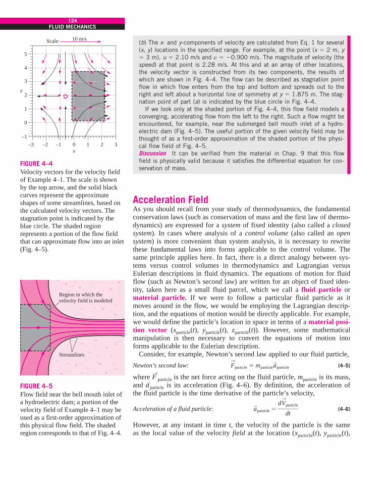
(b) The x- and y-components of velocity are calculated from Eq. 1 for several(x, y) locations in the specified range. For example, at the point (x ! 2 m, y! 3 m), u ! 2.10 m/s and v ! "0.900 m/s. The magnitude of velocity (thespeed) at that point is 2.28 m/s. At this and at an array of other locations,the velocity vector is constructed from its two components, the results ofwhich are shown in Fig. 4–4. The flow can be described as stagnation pointflow in which flow enters from the top and bottom and spreads out to theright and left about a horizontal line of symmetry at y ! 1.875 m. The stag-nation point of part (a) is indicated by the blue circle in Fig. 4–4.

If we look only at the shaded portion of Fig. 4–4, this flow field models aconverging, accelerating flow from the left to the right. Such a flow might beencountered, for example, near the submerged bell mouth inlet of a hydro-electric dam (Fig. 4–5). The useful portion of the given velocity field may bethought of as a first-order approximation of the shaded portion of the physi-cal flow field of Fig. 4–5.Discussion It can be verified from the material in Chap. 9 that this flowfield is physically valid because it satisfies the differential equation for con-servation of mass.

Acceleration FieldAs you should recall from your study of thermodynamics, the fundamentalconservation laws (such as conservation of mass and the first law of thermo-dynamics) are expressed for a system of fixed identity (also called a closedsystem). In cases where analysis of a control volume (also called an opensystem) is more convenient than system analysis, it is necessary to rewritethese fundamental laws into forms applicable to the control volume. Thesame principle applies here. In fact, there is a direct analogy between sys-tems versus control volumes in thermodynamics and Lagrangian versusEulerian descriptions in fluid dynamics. The equations of motion for fluidflow (such as Newton’s second law) are written for an object of fixed iden-tity, taken here as a small fluid parcel, which we call a fluid particle ormaterial particle. If we were to follow a particular fluid particle as itmoves around in the flow, we would be employing the Lagrangian descrip-tion, and the equations of motion would be directly applicable. For example,we would define the particle’s location in space in terms of a material posi-tion vector (xparticle(t), yparticle(t), zparticle(t)). However, some mathematicalmanipulation is then necessary to convert the equations of motion intoforms applicable to the Eulerian description.

Consider, for example, Newton’s second law applied to our fluid particle,

Newton’s second law: (4–5)

where F!

particle is the net force acting on the fluid particle, mparticle is its mass,and a!particle is its acceleration (Fig. 4–6). By definition, the acceleration ofthe fluid particle is the time derivative of the particle’s velocity,

Acceleration of a fluid particle: (4–6)

However, at any instant in time t, the velocity of the particle is the sameas the local value of the velocity field at the location (xparticle(t), yparticle(t),

a!

particle !dV

!particle

dt

F!

particle ! mparticlea!

particle

124FLUID MECHANICS

Scale:

5

4

3

2y

1

0

–1–3 –2 –1 0

x1 2 3

10 m/s

FIGURE 4–4Velocity vectors for the velocity fieldof Example 4–1. The scale is shownby the top arrow, and the solid blackcurves represent the approximateshapes of some streamlines, based onthe calculated velocity vectors. Thestagnation point is indicated by theblue circle. The shaded regionrepresents a portion of the flow fieldthat can approximate flow into an inlet(Fig. 4–5).

Region in which thevelocity field is modeled

Streamlines

FIGURE 4–5Flow field near the bell mouth inlet ofa hydroelectric dam; a portion of thevelocity field of Example 4–1 may beused as a first-order approximation ofthis physical flow field. The shadedregion corresponds to that of Fig. 4–4.

cen72367_ch04.qxd 12/1/04 6:19 PM Page 124

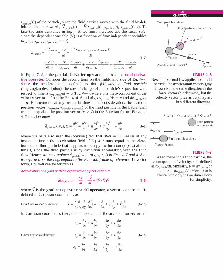
zparticle(t)) of the particle, since the fluid particle moves with the fluid by def-inition. In other words, V

!

particle(t) ! V!

(xparticle(t), yparticle(t), zparticle(t), t). Totake the time derivative in Eq. 4–6, we must therefore use the chain rule,since the dependent variable (V

!) is a function of four independent variables

(xparticle, yparticle, zparticle, and t),

(4–7)

In Eq. 4–7, $ is the partial derivative operator and d is the total deriva-tive operator. Consider the second term on the right-hand side of Eq. 4–7.Since the acceleration is defined as that following a fluid particle(Lagrangian description), the rate of change of the particle’s x-position withrespect to time is dxparticle/dt ! u (Fig. 4–7), where u is the x-component of thevelocity vector defined by Eq. 4–4. Similarly, dyparticle /dt ! v and dzparticle /dt! w. Furthermore, at any instant in time under consideration, the materialposition vector (xparticle, yparticle, zparticle) of the fluid particle in the Lagrangianframe is equal to the position vector (x, y, z) in the Eulerian frame. Equation4–7 thus becomes

(4–8)

where we have also used the (obvious) fact that dt/dt ! 1. Finally, at anyinstant in time t, the acceleration field of Eq. 4–3 must equal the accelera-tion of the fluid particle that happens to occupy the location (x, y, z) at thattime t, since the fluid particle is by definition accelerating with the fluidflow. Hence, we may replace a!particle with a!(x, y, z, t) in Eqs. 4–7 and 4–8 totransform from the Lagrangian to the Eulerian frame of reference. In vectorform, Eq. 4–8 can be written as

Acceleration of a fluid particle expressed as a field variable:

(4–9)

where %!

is the gradient operator or del operator, a vector operator that isdefined in Cartesian coordinates as

Gradient or del operator: (4–10)

In Cartesian coordinates then, the components of the acceleration vector are

Cartesian coordinates: (4–11)

az !$w$t

# u $w$x

# v $w$y

# w $w$z

ay !$v$t

# u $v$x

# v $v$y

# w $v$z

ax !$u$t

# u $u$x

# v $u$y

# w $u$z

§!

! a $

$x,

$

$y, $

$zb ! i

! $

$x# j

! $

$y# k

! $

$z

a!(x, y, z, t) !

dV!

dt!

$V!

$t# (V

!& §

!)V

!

a!

particle(x, y, z, t) !dV

!

dt!

$V!

$t# u

$V!

$x# v

$V!

$y# w

$V!

$z

!$V

!

$t dtdt

#$V

!

$xparticle dxparticle

dt#

$V!

$yparticle dyparticle

dt#

$V!

$zparticle dzparticle

dt

a!

particle !dV

!

particle

dt!

dV!

dt!

dV!(xparticle, yparticle, zparticle, t)

dt

125CHAPTER 4

Vparticle ! V

Fparticle

aparticlemparticle

(xparticle, yparticle, zparticle)

Fluid particle at time t

Fluid particle at time t + dt

! !

!

!

FIGURE 4–6Newton’s second law applied to a fluid

particle; the acceleration vector (grayarrow) is in the same direction as the

force vector (black arrow), but thevelocity vector (blue arrow) may act

in a different direction.

Fluid particle at time t

Fluid particleat time t + dt

(xparticle, yparticle)

(xparticle + dxparticle, yparticle + dyparticle)

dyparticle dxparticle

FIGURE 4–7When following a fluid particle, the

x-component of velocity, u, is definedas dxparticle/dt. Similarly, v ! dyparticle/dt

and w ! dzparticle/dt. Movement isshown here only in two dimensions

for simplicity.

cen72367_ch04.qxd 12/1/04 6:19 PM Page 125

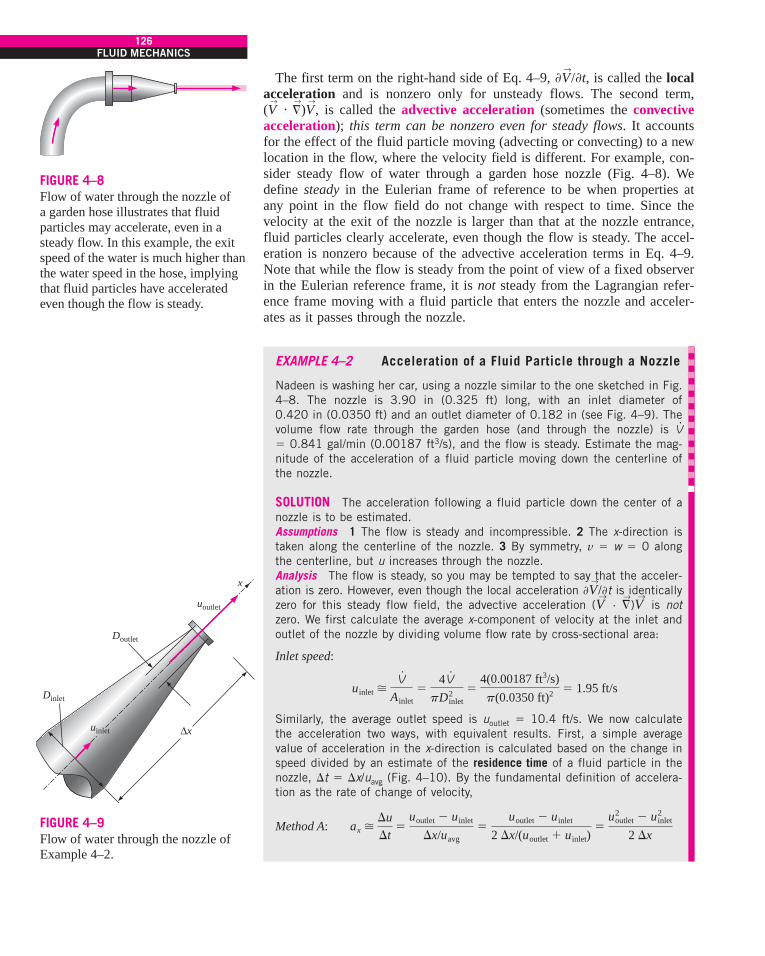
The first term on the right-hand side of Eq. 4–9, $V!

/$t, is called the localacceleration and is nonzero only for unsteady flows. The second term,(V

!· %

!)V

!, is called the advective acceleration (sometimes the convective

acceleration); this term can be nonzero even for steady flows. It accountsfor the effect of the fluid particle moving (advecting or convecting) to a newlocation in the flow, where the velocity field is different. For example, con-sider steady flow of water through a garden hose nozzle (Fig. 4–8). Wedefine steady in the Eulerian frame of reference to be when properties atany point in the flow field do not change with respect to time. Since thevelocity at the exit of the nozzle is larger than that at the nozzle entrance,fluid particles clearly accelerate, even though the flow is steady. The accel-eration is nonzero because of the advective acceleration terms in Eq. 4–9.Note that while the flow is steady from the point of view of a fixed observerin the Eulerian reference frame, it is not steady from the Lagrangian refer-ence frame moving with a fluid particle that enters the nozzle and acceler-ates as it passes through the nozzle.

EXAMPLE 4–2 Acceleration of a Fluid Particle through a Nozzle

Nadeen is washing her car, using a nozzle similar to the one sketched in Fig.4–8. The nozzle is 3.90 in (0.325 ft) long, with an inlet diameter of0.420 in (0.0350 ft) and an outlet diameter of 0.182 in (see Fig. 4–9). Thevolume flow rate through the garden hose (and through the nozzle) is V

.

! 0.841 gal/min (0.00187 ft3/s), and the flow is steady. Estimate the mag-nitude of the acceleration of a fluid particle moving down the centerline ofthe nozzle.

SOLUTION The acceleration following a fluid particle down the center of anozzle is to be estimated.Assumptions 1 The flow is steady and incompressible. 2 The x-direction istaken along the centerline of the nozzle. 3 By symmetry, v ! w ! 0 alongthe centerline, but u increases through the nozzle.Analysis The flow is steady, so you may be tempted to say that the acceler-ation is zero. However, even though the local acceleration $V

!/$t is identically

zero for this steady flow field, the advective acceleration (V!

· %!)V

!is not

zero. We first calculate the average x-component of velocity at the inlet andoutlet of the nozzle by dividing volume flow rate by cross-sectional area:

Inlet speed:

Similarly, the average outlet speed is uoutlet ! 10.4 ft/s. We now calculatethe acceleration two ways, with equivalent results. First, a simple averagevalue of acceleration in the x-direction is calculated based on the change inspeed divided by an estimate of the residence time of a fluid particle in thenozzle, 't ! 'x/uavg (Fig. 4–10). By the fundamental definition of accelera-tion as the rate of change of velocity,

Method A: ax "'u't

!uoutlet " uinlet

'x/uavg!

uoutlet " uinlet

2 'x/(uoutlet # uinlet)!

uoutlet2 " uinlet

2

2 'x

uinlet "V#

Ainlet!

4V#

pD2inlet

!4(0.00187 ft3/s)p(0.0350 ft)2 ! 1.95 ft/s

126FLUID MECHANICS

FIGURE 4–8Flow of water through the nozzle of a garden hose illustrates that fluidparticles may accelerate, even in asteady flow. In this example, the exitspeed of the water is much higher thanthe water speed in the hose, implyingthat fluid particles have acceleratedeven though the flow is steady.

Doutlet

Dinlet

uoutlet

x

"xuinlet

FIGURE 4–9Flow of water through the nozzle ofExample 4–2.

cen72367_ch04.qxd 12/1/04 6:19 PM Page 126

The second method uses the equation for acceleration field components inCartesian coordinates, Eq. 4–11,

Method B:

Steady v ! 0 along centerline w ! 0 along centerline

Here we see that only one advective term is nonzero. We approximate theaverage speed through the nozzle as the average of the inlet and outletspeeds, and we use a first-order finite difference approximation (Fig. 4–11) forthe average value of derivative $u/$x through the centerline of the nozzle:

The result of method B is identical to that of method A. Substitution of thegiven values yields

Axial acceleration:

Discussion Fluid particles are accelerated through the nozzle at nearly fivetimes the acceleration of gravity (almost five g’s)! This simple exampleclearly illustrates that the acceleration of a fluid particle can be nonzero,even in steady flow. Note that the acceleration is actually a point function,whereas we have estimated a simple average acceleration through the entirenozzle.

Material DerivativeThe total derivative operator d/dt in Eq. 4–9 is given a special name, thematerial derivative; some authors also assign to it a special notation, D/Dt,in order to emphasize that it is formed by following a fluid particle as itmoves through the flow field (Fig. 4–12). Other names for the materialderivative include total, particle, Lagrangian, Eulerian, and substantialderivative.

Material derivative: (4–12)

When we apply the material derivative of Eq. 4–12 to the velocity field, theresult is the acceleration field as expressed by Eq. 4–9, which is thus some-times called the material acceleration.

Material acceleration: (4–13)

Equation 4–12 can also be applied to other fluid properties besides velocity,both scalars and vectors. For example, the material derivative of pressurecan be written as

Material derivative of pressure: (4–14)DPDt

!dPdt

!$P$t

# (V!

& §!

)P

a!(x, y, z, t) !

DV!

Dt!

dV!

dt!

$V!

$t# (V

!& §

!)V

!

DDt

!ddt

!$

$t# (V

!& §

!)

ax "u2

outlet " u2inlet

2 'x!

(10.4 ft/s)2 " (1.95 ft/s)2

2(0.325 ft)! 160 ft/s2

ax "uoutlet # uinlet

2 uoutlet " uinlet

'x!

uoutlet2 " uinlet

2

2 'x

ax !$u$t

# u $u$x

# v $u$y

# w $u$z

" uavg'u'x

127CHAPTER 4

Fluid particleat time t + "t

Fluid particleat time t

x

"x

FIGURE 4–10Residence time 't is defined as the

time it takes for a fluid particle totravel through the nozzle from inlet

to outlet (distance 'x).

q

x

"x

# "q"x

dqdx

"q

FIGURE 4–11A first-order finite difference

approximation for derivative dq/dxis simply the change in dependentvariable (q) divided by the change

in independent variable (x).

t

t + dt

t + 2 dtt + 3 dt

FIGURE 4–12The material derivative D/Dt is

defined by following a fluid particle as it moves throughout the flow field.In this illustration, the fluid particle is

accelerating to the right as it moves up and to the right.

$%&F $%&0 0 0— — —

cen72367_ch04.qxd 12/1/04 6:19 PM Page 127

Equation 4–14 represents the time rate of change of pressure following afluid particle as it moves through the flow and contains both local(unsteady) and advective components (Fig. 4–13).

EXAMPLE 4–3 Material Acceleration of a Steady Velocity Field

Consider the steady, incompressible, two-dimensional velocity field of Example4–1. (a) Calculate the material acceleration at the point (x ! 2 m, y ! 3 m).(b) Sketch the material acceleration vectors at the same array of x- and y-values as in Example 4–1.

SOLUTION For the given velocity field, the material acceleration vector is tobe calculated at a particular point and plotted at an array of locations in theflow field.Assumptions 1 The flow is steady and incompressible. 2 The flow is two-dimensional, implying no z-component of velocity and no variation of u or vwith z.Analysis (a) Using the velocity field of Eq. 1 of Example 4–1 and the equa-tion for material acceleration components in Cartesian coordinates (Eq.4–11), we write expressions for the two nonzero components of the accelera-tion vector:

and

At the point (x ! 2 m, y ! 3 m), ax ! 1.68 m/s2 and ay ! 0.720 m/s2.(b) The equations in part (a) are applied to an array of x- and y-values in theflow domain within the given limits, and the acceleration vectors are plottedin Fig. 4–14.Discussion The acceleration field is nonzero, even though the flow issteady. Above the stagnation point (above y ! 1.875 m), the accelerationvectors plotted in Fig. 4–14 point upward, increasing in magnitude awayfrom the stagnation point. To the right of the stagnation point (to the right ofx ! "0.625 m), the acceleration vectors point to the right, again increasingin magnitude away from the stagnation point. This agrees qualitatively withthe velocity vectors of Fig. 4–4 and the streamlines sketched in Fig. 4–14;namely, in the upper-right portion of the flow field, fluid particles are accel-erated in the upper-right direction and therefore veer in the counterclockwisedirection due to centripetal acceleration toward the upper right. The flowbelow y ! 1.875 m is a mirror image of the flow above this symmetry line,and flow to the left of x ! "0.625 m is a mirror image of the flow to theright of this symmetry line.

! 0 # (0.5 # 0.8x)(0) # (1.5 " 0.8y)("0.8) # 0 ! ("1.2 # 0.64y) m/s2

ay !$v$t

# u $v$x

# v $v$y

# w $v$z

! 0 # (0.5 # 0.8x)(0.8) # (15 " 0.8y)(0) # 0 ! (0.4 # 0.64x) m/s2

ax !$u$t

# u $u$x

# v $u$y

# w $u$z

128FLUID MECHANICS

$$t

LocalLocal

= +DDtDt

MaterialMaterialderivativederivative

V V & %& %( )

AdvectiveAdvective

! !

FIGURE 4–13The material derivative D/Dt iscomposed of a local or unsteady partand a convective or advective part.

Scale:

5

4

3

2y

1

0

–1–3 –2 –1 0

x1 2 3

10 m/s2

FIGURE 4–14Acceleration vectors for the velocityfield of Examples 4–1 and 4–3. Thescale is shown by the top arrow,and the solid black curves representthe approximate shapes of somestreamlines, based on the calculatedvelocity vectors (see Fig. 4–4). Thestagnation point is indicated by the blue circle.

$ ' ' % ' ' & $ ' % ' &

$ ' ' % ' ' &$ ' % ' &

cen72367_ch04.qxd 12/1/04 6:19 PM Page 128

4–2 ! FUNDAMENTALS OF FLOW VISUALIZATIONWhile quantitative study of fluid dynamics requires advanced mathematics,much can be learned from flow visualization—the visual examination offlow field features. Flow visualization is useful not only in physical experi-ments (Fig. 4–15), but in numerical solutions as well [computational fluiddynamics (CFD)]. In fact, the very first thing an engineer using CFD doesafter obtaining a numerical solution is simulate some form of flow visual-ization, so that he or she can see the “whole picture” rather than merely alist of numbers and quantitative data. Why? Because the human mind isdesigned to rapidly process an incredible amount of visual information; asthey say, a picture is worth a thousand words. There are many types of flowpatterns that can be visualized, both physically (experimentally) and/orcomputationally.

Streamlines and StreamtubesA streamline is a curve that is everywhere tangent to the instantaneous localvelocity vector.

Streamlines are useful as indicators of the instantaneous direction of fluidmotion throughout the flow field. For example, regions of recirculating flowand separation of a fluid off of a solid wall are easily identified by thestreamline pattern. Streamlines cannot be directly observed experimentallyexcept in steady flow fields, in which they are coincident with pathlines andstreaklines, to be discussed next. Mathematically, however, we can write asimple expression for a streamline based on its definition.

Consider an infinitesimal arc length dr! ! dxi!

# dyj!

# dzk!

along astreamline; dr! must be parallel to the local velocity vector V

!! ui

!# vj

!# wk

!

by definition of the streamline. By simple geometric arguments using simi-lar triangles, we know that the components of dr! must be proportional tothose of V

!(Fig. 4–16). Hence,

Equation for a streamline: (4–15)

where dr is the magnitude of dr! and V is the speed, the magnitude of V!

.Equation 4–15 is illustrated in two dimensions for simplicity in Fig. 4–16.For a known velocity field, we can integrate Eq. 4–15 to obtain equationsfor the streamlines. In two dimensions, (x, y), (u, v), the following differen-tial equation is obtained:

Streamline in the xy-plane: (4–16)

In some simple cases, Eq. 4–16 may be solvable analytically; in the generalcase, it must be solved numerically. In either case, an arbitrary constant ofintegration appears, and the family of curves that satisfy Eq. 4–16 representsstreamlines of the flow field.

ady

dxb

along a streamline!

vu

drV

!dxu

!dyv

!dzw

129CHAPTER 4

FIGURE 4–15Spinning baseball.

The late F. N. M. Brown devotedmany years to developing and using

smoke visualization in wind tunnels atthe University of Notre Dame. Here

the flow speed is about 77 ft/s and theball is rotated at 630 rpm.

Photograph courtesy of T. J. Mueller.

y

x

Point (x, y)

Streamline

Point (x + dx, y + dy)

dx

dy

u

v

V

dr!

!

FIGURE 4–16For two-dimensional flow in the xy-

plane, arc length dr! ! (dx, dy) along a streamline is everywhere tangent to

the local instantaneous velocity vectorV!

! (u, v).

cen72367_ch04.qxd 12/1/04 6:19 PM Page 129

EXAMPLE 4–4 Streamlines in the xy-Plane—An AnalyticalSolution

For the steady, incompressible, two-dimensional velocity field of Example4–1, plot several streamlines in the right half of the flow (x ( 0) and com-pare to the velocity vectors plotted in Fig. 4–4.

SOLUTION An analytical expression for streamlines is to be generated andplotted in the upper-right quadrant.Assumptions 1 The flow is steady and incompressible. 2 The flow is two-dimensional, implying no z-component of velocity and no variation of u or vwith z.Analysis Equation 4–16 is applicable here; thus, along a streamline,

We solve this differential equation by separation of variables:

After some algebra (which we leave to the reader), we solve for y as a func-tion of x along a streamline,

where C is a constant of integration that can be set to various values in orderto plot the streamlines. Several streamlines of the given flow field are shownin Fig. 4–17.Discussion The velocity vectors of Fig. 4–4 are superimposed on thestreamlines of Fig. 4–17; the agreement is excellent in the sense that thevelocity vectors point everywhere tangent to the streamlines. Note that speedcannot be determined directly from the streamlines alone.

A streamtube consists of a bundle of streamlines (Fig. 4–18), much likea communications cable consists of a bundle of fiber-optic cables. Sincestreamlines are everywhere parallel to the local velocity, fluid cannot cross astreamline by definition. By extension, fluid within a streamtube mustremain there and cannot cross the boundary of the streamtube. You mustkeep in mind that both streamlines and streamtubes are instantaneous quan-tities, defined at a particular instant in time according to the velocity field atthat instant. In an unsteady flow, the streamline pattern may change signifi-cantly with time. Nevertheless, at any instant in time, the mass flow ratepassing through any cross-sectional slice of a given streamtube must remainthe same. For example, in a converging portion of an incompressible flowfield, the diameter of the streamtube must decrease as the velocity increasesso as to conserve mass (Fig. 4–19a). Likewise, the streamtube diameterincreases in diverging portions of the incompressible flow (Fig. 4–19b).

PathlinesA pathline is the actual path traveled by an individual fluid particle over sometime period.

y !C

0.8(0.5 # 0.8x)# 1.875

dy

1.5 " 0.8y!

dx0.5 # 0.8x

! # dy

1.5 " 0.8y! # dx

0.5 # 0.8x

dy

dx!

1.5 " 0.8y

0.5 # 0.8x

130FLUID MECHANICS

5

4

3

2y

1

0

–10 1 2 3

x4 5

FIGURE 4–17Streamlines (solid black curves) forthe velocity field of Example 4–4;velocity vectors of Fig. 4–4 (bluearrows) are superimposed forcomparison.

Streamlines

Streamtube

FIGURE 4–18A streamtube consists of a bundle ofindividual streamlines.

cen72367_ch04.qxd 12/1/04 6:19 PM Page 130

Pathlines are the easiest of the flow patterns to understand. A pathline is aLagrangian concept in that we simply follow the path of an individual fluidparticle as it moves around in the flow field (Fig. 4–20). Thus, a pathline isthe same as the fluid particle’s material position vector (xparticle(t), yparticle(t),zparticle(t)), discussed in Section 4–1, traced out over some finite time inter-val. In a physical experiment, you can imagine a tracer fluid particle that ismarked somehow—either by color or brightness—such that it is easily dis-tinguishable from surrounding fluid particles. Now imagine a camera withthe shutter open for a certain time period, tstart ) t ) tend, in which the parti-cle’s path is recorded; the resulting curve is called a pathline. An intriguingexample is shown in Fig. 4–21 for the case of waves moving along the sur-face of water in a tank. Neutrally buoyant white tracer particles are sus-pended in the water, and a time-exposure photograph is taken for one com-plete wave period. The result is pathlines that are elliptical in shape,showing that fluid particles bob up and down and forward and backward,but return to their original position upon completion of one wave period;there is no net forward motion. You may have experienced something simi-lar while bobbing up and down on ocean waves.

131CHAPTER 4

(b)(a)

FIGURE 4–19In an incompressible flow field, a

streamtube (a) decreases in diameteras the flow accelerates or convergesand (b) increases in diameter as the

flow decelerates or diverges.

A modern experimental technique called particle image velocimetry(PIV) utilizes particle pathlines to measure the velocity field over an entireplane in a flow (Adrian, 1991). (Recent advances also extend the techniqueto three dimensions.) In PIV, tiny tracer particles are suspended in the fluid,much like in Fig. 4–21. However, the flow is illuminated by two flashes oflight (usually from a laser as in Fig. 4–22) to produce two bright spots onthe film or photosensor for each moving particle. Then, both the magnitudeand direction of the velocity vector at each particle location can be inferred,assuming that the tracer particles are small enough that they move with thefluid. Modern digital photography and fast computers have enabled PIV tobe performed rapidly enough so that unsteady features of a flow field canalso be measured. PIV is discussed in more detail in Chap. 8.

Fluid particle at t = tstart

Fluid particle at t = tend

Fluid particle at someintermediate time

Pathline

FIGURE 4–20A pathline is formed by following the

actual path of a fluid particle.

FIGURE 4–22PIV applied to a model car in a wind

tunnel.Courtesy Dantec Dynamics, Inc.

Used by permission.

FIGURE 4–21Pathlines produced by white tracer

particles suspended in water andcaptured by time-exposure

photography; as waves passhorizontally, each particle moves

in an elliptical path during one wave period.

Wallet, A. & Ruellan, F. 1950, La Houille Blanche 5:483–489. Used by permission.

cen72367_ch04.qxd 12/1/04 6:19 PM Page 131

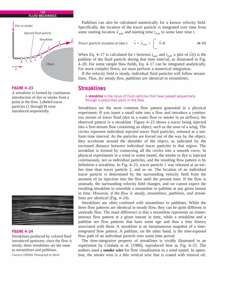
Pathlines can also be calculated numerically for a known velocity field.Specifically, the location of the tracer particle is integrated over time fromsome starting location x!start and starting time tstart to some later time t.

Tracer particle location at time t: (4–17)

When Eq. 4–17 is calculated for t between tstart and tend, a plot of x!

(t) is thepathline of the fluid particle during that time interval, as illustrated in Fig.4–20. For some simple flow fields, Eq. 4–17 can be integrated analytically.For more complex flows, we must perform a numerical integration.

If the velocity field is steady, individual fluid particles will follow stream-lines. Thus, for steady flow, pathlines are identical to streamlines.

StreaklinesA streakline is the locus of fluid particles that have passed sequentiallythrough a prescribed point in the flow.

Streaklines are the most common flow pattern generated in a physicalexperiment. If you insert a small tube into a flow and introduce a continu-ous stream of tracer fluid (dye in a water flow or smoke in an airflow), theobserved pattern is a streakline. Figure 4–23 shows a tracer being injectedinto a free-stream flow containing an object, such as the nose of a wing. Thecircles represent individual injected tracer fluid particles, released at a uni-form time interval. As the particles are forced out of the way by the object,they accelerate around the shoulder of the object, as indicated by theincreased distance between individual tracer particles in that region. Thestreakline is formed by connecting all the circles into a smooth curve. Inphysical experiments in a wind or water tunnel, the smoke or dye is injectedcontinuously, not as individual particles, and the resulting flow pattern is bydefinition a streakline. In Fig. 4–23, tracer particle 1 was released at an ear-lier time than tracer particle 2, and so on. The location of an individualtracer particle is determined by the surrounding velocity field from themoment of its injection into the flow until the present time. If the flow isunsteady, the surrounding velocity field changes, and we cannot expect theresulting streakline to resemble a streamline or pathline at any given instantin time. However, if the flow is steady, streamlines, pathlines, and streak-lines are identical (Fig. 4–24).

Streaklines are often confused with streamlines or pathlines. While thethree flow patterns are identical in steady flow, they can be quite different inunsteady flow. The main difference is that a streamline represents an instan-taneous flow pattern at a given instant in time, while a streakline and apathline are flow patterns that have some age and thus a time historyassociated with them. A streakline is an instantaneous snapshot of a time-integrated flow pattern. A pathline, on the other hand, is the time-exposedflow path of an individual particle over some time period.

The time-integrative property of streaklines is vividly illustrated in anexperiment by Cimbala et al. (1988), reproduced here as Fig. 4–25. Theauthors used a smoke wire for flow visualization in a wind tunnel. In opera-tion, the smoke wire is a thin vertical wire that is coated with mineral oil.

x!

! x!

start # #t

tstart

V! dt

132FLUID MECHANICS

V

Streakline

Object8 7 6 5

4

3

21

Injected fluid particle

Dye or smoke

FIGURE 4–23A streakline is formed by continuousintroduction of dye or smoke from apoint in the flow. Labeled tracerparticles (1 through 8) wereintroduced sequentially.

FIGURE 4–24Streaklines produced by colored fluidintroduced upstream; since the flow issteady, these streaklines are the sameas streamlines and pathlines. Courtesy ONERA. Photograph by Werlé.

cen72367_ch04.qxd 12/1/04 6:19 PM Page 132

The oil breaks up into beads along the length of the wire due to surface ten-sion effects. When an electric current heats the wire, each little bead of oilproduces a streakline of smoke. In Fig. 4–25a, streaklines are introducedfrom a smoke wire located just downstream of a circular cylinder of diameterD aligned normal to the plane of view. (When multiple streaklines are intro-duced along a line, as in Fig. 4–25, we refer to this as a rake of streaklines.)The Reynolds number of the flow is Re ! rVD/m ! 93. Because of unsteadyvortices shed in an alternating pattern from the cylinder, the smoke collectsinto a clearly defined pattern called a Kármán vortex street.

From Fig. 4–25a alone, one may think that the shed vortices continue toexist to several hundred diameters downstream of the cylinder. However, thestreakline pattern of this figure is misleading! In Fig. 4–25b, the smoke wireis placed 150 diameters downstream of the cylinder. The resulting streaklinesare straight, indicating that the shed vortices have in reality disappeared bythis downstream distance. The flow is steady and parallel at this location, andthere are no more vortices; viscous diffusion has caused adjacent vortices ofopposite sign to cancel each other out by around 100 cylinder diameters. Thepatterns of Fig. 4–25a near x/D ! 150 are merely remnants of the vortexstreet that existed upstream. The streaklines of Fig. 4–25b, however, showthe correct features of the flow at that location. The streaklines generated atx/D ! 150 are identical to streamlines or pathlines in that region of theflow—straight, nearly horizontal lines—since the flow is steady there.

For a known velocity field, a streakline can be generated numerically,although with some difficulty. One needs to follow the paths of a continuousstream of tracer particles from the time of their injection into the flow untilthe present time, using Eq. 4–17. Mathematically, the location of a tracerparticle is integrated over time from the time of its injection tinject to the present time tpresent. Equation 4–17 becomes

Integrated tracer particle location: (4–18)x!

! x!

injection # #tpresent

tinject

V!

dt

133CHAPTER 4

(a)

(b)

0 50

Cylinder

x/D

100 150 200 250

Cylinder

FIGURE 4–25Smoke streaklines introduced by a smoke wire at two different locations in thewake of a circular cylinder: (a) smoke wire just downstream of the cylinder and(b) smoke wire located at x/D = 150. The time-integrative nature of streaklines is clearly seen by comparing the two photographs.Photos by John M. Cimbala.

cen72367_ch04.qxd 12/1/04 6:19 PM Page 133

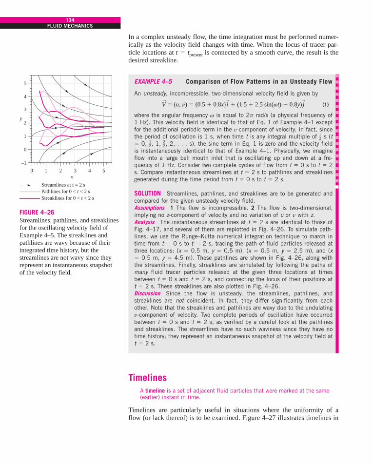
134FLUID MECHANICS

5

4

3

2y

1

0

–10

x1 2

Streamlines at t = 2 s

3 4 5

Pathlines for 0 < t < 2 sStreaklines for 0 < t < 2 s

FIGURE 4–26Streamlines, pathlines, and streaklinesfor the oscillating velocity field ofExample 4–5. The streaklines andpathlines are wavy because of theirintegrated time history, but thestreamlines are not wavy since theyrepresent an instantaneous snapshot of the velocity field.

In a complex unsteady flow, the time integration must be performed numer-ically as the velocity field changes with time. When the locus of tracer par-ticle locations at t ! tpresent is connected by a smooth curve, the result is thedesired streakline.

EXAMPLE 4–5 Comparison of Flow Patterns in an Unsteady Flow

An unsteady, incompressible, two-dimensional velocity field is given by

(1)

where the angular frequency v is equal to 2p rad/s (a physical frequency of1 Hz). This velocity field is identical to that of Eq. 1 of Example 4–1 exceptfor the additional periodic term in the v-component of velocity. In fact, sincethe period of oscillation is 1 s, when time t is any integral multiple of s (t! 0, , 1, , 2, . . . s), the sine term in Eq. 1 is zero and the velocity fieldis instantaneously identical to that of Example 4–1. Physically, we imagineflow into a large bell mouth inlet that is oscillating up and down at a fre-quency of 1 Hz. Consider two complete cycles of flow from t ! 0 s to t ! 2s. Compare instantaneous streamlines at t ! 2 s to pathlines and streaklinesgenerated during the time period from t ! 0 s to t ! 2 s.

SOLUTION Streamlines, pathlines, and streaklines are to be generated andcompared for the given unsteady velocity field.Assumptions 1 The flow is incompressible. 2 The flow is two-dimensional,implying no z-component of velocity and no variation of u or v with z.Analysis The instantaneous streamlines at t ! 2 s are identical to those ofFig. 4–17, and several of them are replotted in Fig. 4–26. To simulate path-lines, we use the Runge–Kutta numerical integration technique to march intime from t ! 0 s to t ! 2 s, tracing the path of fluid particles released atthree locations: (x ! 0.5 m, y ! 0.5 m), (x ! 0.5 m, y ! 2.5 m), and (x! 0.5 m, y ! 4.5 m). These pathlines are shown in Fig. 4–26, along withthe streamlines. Finally, streaklines are simulated by following the paths ofmany fluid tracer particles released at the given three locations at timesbetween t ! 0 s and t ! 2 s, and connecting the locus of their positions att ! 2 s. These streaklines are also plotted in Fig. 4–26.Discussion Since the flow is unsteady, the streamlines, pathlines, andstreaklines are not coincident. In fact, they differ significantly from eachother. Note that the streaklines and pathlines are wavy due to the undulatingv-component of velocity. Two complete periods of oscillation have occurredbetween t ! 0 s and t ! 2 s, as verified by a careful look at the pathlinesand streaklines. The streamlines have no such waviness since they have no time history; they represent an instantaneous snapshot of the velocity field att ! 2 s.

TimelinesA timeline is a set of adjacent fluid particles that were marked at the same(earlier) instant in time.

Timelines are particularly useful in situations where the uniformity of aflow (or lack thereof) is to be examined. Figure 4–27 illustrates timelines in

32

12

12

V!

! (u, v) ! (0.5 # 0.8x) i!

# (1.5 # 2.5 sin(vt) " 0.8y) j!

cen72367_ch04.qxd 12/1/04 6:19 PM Page 134

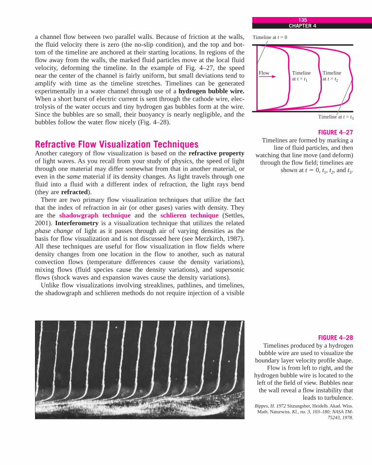
a channel flow between two parallel walls. Because of friction at the walls,the fluid velocity there is zero (the no-slip condition), and the top and bot-tom of the timeline are anchored at their starting locations. In regions of theflow away from the walls, the marked fluid particles move at the local fluidvelocity, deforming the timeline. In the example of Fig. 4–27, the speednear the center of the channel is fairly uniform, but small deviations tend toamplify with time as the timeline stretches. Timelines can be generatedexperimentally in a water channel through use of a hydrogen bubble wire.When a short burst of electric current is sent through the cathode wire, elec-trolysis of the water occurs and tiny hydrogen gas bubbles form at the wire.Since the bubbles are so small, their buoyancy is nearly negligible, and thebubbles follow the water flow nicely (Fig. 4–28).

Refractive Flow Visualization TechniquesAnother category of flow visualization is based on the refractive propertyof light waves. As you recall from your study of physics, the speed of lightthrough one material may differ somewhat from that in another material, oreven in the same material if its density changes. As light travels through onefluid into a fluid with a different index of refraction, the light rays bend(they are refracted).

There are two primary flow visualization techniques that utilize the factthat the index of refraction in air (or other gases) varies with density. Theyare the shadowgraph technique and the schlieren technique (Settles,2001). Interferometry is a visualization technique that utilizes the relatedphase change of light as it passes through air of varying densities as thebasis for flow visualization and is not discussed here (see Merzkirch, 1987).All these techniques are useful for flow visualization in flow fields wheredensity changes from one location in the flow to another, such as naturalconvection flows (temperature differences cause the density variations),mixing flows (fluid species cause the density variations), and supersonicflows (shock waves and expansion waves cause the density variations).

Unlike flow visualizations involving streaklines, pathlines, and timelines,the shadowgraph and schlieren methods do not require injection of a visible

135CHAPTER 4

Timeline at t = 0

Timeline at t = t1

Timeline at t = t2

Timeline at t = t3

Flow

FIGURE 4–27Timelines are formed by marking a

line of fluid particles, and thenwatching that line move (and deform)

through the flow field; timelines areshown at t ! 0, t1, t2, and t3.

FIGURE 4–28Timelines produced by a hydrogen

bubble wire are used to visualize theboundary layer velocity profile shape.

Flow is from left to right, and thehydrogen bubble wire is located to theleft of the field of view. Bubbles nearthe wall reveal a flow instability that

leads to turbulence. Bippes, H. 1972 Sitzungsber, Heidelb. Akad. Wiss.

Math. Naturwiss. Kl., no. 3, 103–180; NASA TM-75243, 1978.

cen72367_ch04.qxd 12/1/04 6:19 PM Page 135

tracer (smoke or dye). Rather, density differences and the refractive propertyof light provide the necessary means for visualizing regions of activity inthe flow field, allowing us to “see the invisible.” The image (a shadow-gram) produced by the shadowgraph method is formed when the refractedrays of light rearrange the shadow cast onto a viewing screen or camerafocal plane, causing bright or dark patterns to appear in the shadow. Thedark patterns indicate the location where the refracted rays originate, whilethe bright patterns mark where these rays end up, and can be misleading. Asa result, the dark regions are less distorted than the bright regions and aremore useful in the interpretation of the shadowgram. In the shadowgram ofFig. 4–29, for example, we can be confident of the shape and position of thebow shock wave (the dark band), but the refracted bright light has distortedthe front of the sphere’s shadow.

A shadowgram is not a true optical image; it is, after all, merely ashadow. A schlieren image, however, involves lenses (or mirrors) and aknife edge or other cutoff device to block the refracted light and is a truefocused optical image. Schlieren imaging is more complicated to set up thanis shadowgraphy (see Settles, 2001, for details) but has a number of advan-tages. For example, a schlieren image does not suffer from optical distortionby the refracted light rays. Schlieren imaging is also more sensitive to weakdensity gradients such as those caused by natural convection (Fig. 4–30) orby gradual phenomena like expansion fans in supersonic flow. Colorschlieren imaging techniques have also been developed. Finally, one canadjust more components in a schlieren setup, such as the location, orienta-tion, and type of the cutoff device, in order to produce an image that is mostuseful for the problem at hand.

Surface Flow Visualization TechniquesFinally, we briefly mention some flow visualization techniques that are use-ful along solid surfaces. The direction of fluid flow immediately above asolid surface can be visualized with tufts—short, flexible strings glued tothe surface at one end that point in the flow direction. Tufts are especiallyuseful for locating regions of flow separation, where the flow direction sud-denly reverses.

A technique called surface oil visualization can be used for the samepurpose—oil placed on the surface forms streaks that indicate the directionof flow. If it rains lightly when your car is dirty (especially in the winterwhen salt is on the roads), you may have noticed streaks along the hood andsides of the car, or even on the windshield. This is similar to what isobserved with surface oil visualization.

Lastly, there are pressure-sensitive and temperature-sensitive paints thatenable researchers to observe the pressure or temperature distribution alongsolid surfaces.

4–3 ! PLOTS OF FLUID FLOW DATARegardless of how the results are obtained (analytically, experimentally, orcomputationally), it is usually necessary to plot flow data in ways thatenable the reader to get a feel for how the flow properties vary in timeand/or space. You are already familiar with time plots, which are especially

136FLUID MECHANICS

FIGURE 4–29Shadowgram of a 14.3 mm sphere infree flight through air at Ma ! 3.0. A shock wave is clearly visible in theshadow as a dark band that curvesaround the sphere and is called a bow wave (see Chap. 12). A. C. Charters, Air Flow Branch, U.S. ArmyBallistic Research Laboratory.

FIGURE 4–30Schlieren image of natural convectiondue to a barbeque grill. G. S. Settles, Gas Dynamics Lab, Penn StateUniversity. Used by permission.

cen72367_ch04.qxd 12/1/04 6:19 PM Page 136

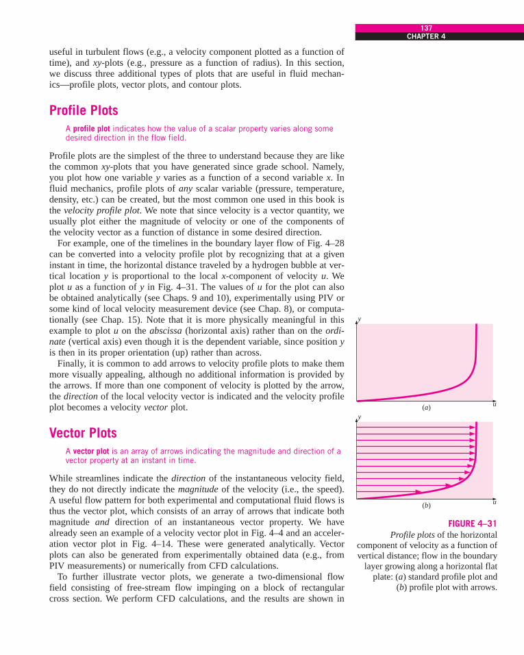
useful in turbulent flows (e.g., a velocity component plotted as a function oftime), and xy-plots (e.g., pressure as a function of radius). In this section,we discuss three additional types of plots that are useful in fluid mechan-ics—profile plots, vector plots, and contour plots.

Profile PlotsA profile plot indicates how the value of a scalar property varies along somedesired direction in the flow field.

Profile plots are the simplest of the three to understand because they are likethe common xy-plots that you have generated since grade school. Namely,you plot how one variable y varies as a function of a second variable x. Influid mechanics, profile plots of any scalar variable (pressure, temperature,density, etc.) can be created, but the most common one used in this book isthe velocity profile plot. We note that since velocity is a vector quantity, weusually plot either the magnitude of velocity or one of the components ofthe velocity vector as a function of distance in some desired direction.

For example, one of the timelines in the boundary layer flow of Fig. 4–28can be converted into a velocity profile plot by recognizing that at a giveninstant in time, the horizontal distance traveled by a hydrogen bubble at ver-tical location y is proportional to the local x-component of velocity u. Weplot u as a function of y in Fig. 4–31. The values of u for the plot can alsobe obtained analytically (see Chaps. 9 and 10), experimentally using PIV orsome kind of local velocity measurement device (see Chap. 8), or computa-tionally (see Chap. 15). Note that it is more physically meaningful in thisexample to plot u on the abscissa (horizontal axis) rather than on the ordi-nate (vertical axis) even though it is the dependent variable, since position yis then in its proper orientation (up) rather than across.

Finally, it is common to add arrows to velocity profile plots to make themmore visually appealing, although no additional information is provided bythe arrows. If more than one component of velocity is plotted by the arrow,the direction of the local velocity vector is indicated and the velocity profileplot becomes a velocity vector plot.

Vector PlotsA vector plot is an array of arrows indicating the magnitude and direction of avector property at an instant in time.

While streamlines indicate the direction of the instantaneous velocity field,they do not directly indicate the magnitude of the velocity (i.e., the speed).A useful flow pattern for both experimental and computational fluid flows isthus the vector plot, which consists of an array of arrows that indicate bothmagnitude and direction of an instantaneous vector property. We havealready seen an example of a velocity vector plot in Fig. 4–4 and an acceler-ation vector plot in Fig. 4–14. These were generated analytically. Vectorplots can also be generated from experimentally obtained data (e.g., fromPIV measurements) or numerically from CFD calculations.

To further illustrate vector plots, we generate a two-dimensional flowfield consisting of free-stream flow impinging on a block of rectangularcross section. We perform CFD calculations, and the results are shown in

137CHAPTER 4

y

(a) u

y

(b) u

FIGURE 4–31Profile plots of the horizontal

component of velocity as a function ofvertical distance; flow in the boundary

layer growing along a horizontal flatplate: (a) standard profile plot and

(b) profile plot with arrows.

cen72367_ch04.qxd 12/1/04 6:19 PM Page 137

Fig. 4–32. Note that this flow is by nature turbulent and unsteady, but onlythe long-time averaged results are calculated and displayed here. Stream-lines are plotted in Fig. 4–32a; a view of the entire block and a large portionof its wake is shown. The closed streamlines above and below the symmetryplane indicate large recirculating eddies, one above and one below the lineof symmetry. A velocity vector plot is shown in Fig. 4–32b. (Only the upperhalf of the flow is shown because of symmetry.) It is clear from this plotthat the flow accelerates around the upstream corner of the block, so muchso in fact that the boundary layer cannot negotiate the sharp corner and sep-arates off the block, producing the large recirculating eddies downstream ofthe block. (Note that these velocity vectors are time-averaged values; theinstantaneous vectors change in both magnitude and direction with time asvortices are shed from the body, similar to those of Fig. 4–25a.) A close-upview of the separated flow region is plotted in Fig. 4–32c, where we verifythe reverse flow in the lower half of the large recirculating eddy.

Modern CFD codes and postprocessors can add color to a vector plot. Forexample, the vectors can be colored according to some other flow propertysuch as pressure (red for high pressure and blue for low pressure) or tem-perature (red for hot and blue for cold). In this manner, one can easily visu-alize not only the magnitude and direction of the flow, but other propertiesas well, simultaneously.

Contour PlotsA contour plot shows curves of constant values of a scalar property (ormagnitude of a vector property) at an instant in time.

If you do any hiking, you are familiar with contour maps of mountain trails.The maps consist of a series of closed curves, each indicating a constantelevation or altitude. Near the center of a group of such curves is the mountain peak or valley; the actual peak or valley is a point on the mapshowing the highest or lowest elevation. Such maps are useful in that notonly do you get a bird’s-eye view of the streams and trails, etc., but you canalso easily see your elevation and where the trail is flat or steep. In fluidmechanics, the same principle is applied to various scalar flow properties;contour plots (also called isocontour plots) are generated of pressure, tem-perature, velocity magnitude, species concentration, properties of turbu-lence, etc. A contour plot can quickly reveal regions of high (or low) valuesof the flow property being studied.

A contour plot may consist simply of curves indicating various levels ofthe property; this is called a contour line plot. Alternatively, the contourscan be filled in with either colors or shades of gray; this is called a filledcontour plot. An example of pressure contours is shown in Fig. 4–33 forthe same flow as in Fig. 4–32. In Fig. 4–33a, filled contours are shownusing shades of gray to identify regions of different pressure levels—darkregions indicate low pressure and light regions indicate high pressure. It isclear from this figure that the pressure is highest at the front face of theblock and lowest along the top of the block in the separated zone. The pres-sure is also low in the wake of the block, as expected. In Fig. 4–33b, thesame pressure contours are shown, but as a contour line plot with labeledlevels of gage pressure in units of pascals.

138FLUID MECHANICS

Recirculating eddy

Symmetry plane

(a)

(b)

(c)

Symmetry plane

Block

Block

FLOWFLOW

Block

FLOWFLOW

FIGURE 4–32Results of CFD calculations of flowimpinging on a block; (a) streamlines,(b) velocity vector plot of the upperhalf of the flow, and (c) velocity vectorplot, close-up view revealing moredetails.

cen72367_ch04.qxd 12/1/04 6:19 PM Page 138

In CFD, contour plots are often displayed in vivid colors with red usuallyindicating the highest value of the scalar and blue the lowest. A healthyhuman eye can easily spot a red or blue region and thus locate regions ofhigh or low value of the flow property. Because of the pretty pictures produced by CFD, computational fluid dynamics is sometimes given thenickname “colorful fluid dynamics.”

4–4 ! OTHER KINEMATIC DESCRIPTIONS

Types of Motion or Deformation of Fluid ElementsIn fluid mechanics, as in solid mechanics, an element may undergo fourfundamental types of motion or deformation, as illustrated in two dimen-sions in Fig. 4–34: (a) translation, (b) rotation, (c) linear strain (some-times called extensional strain), and (d) shear strain. The study of fluiddynamics is further complicated by the fact that all four types of motion ordeformation usually occur simultaneously. Because fluid elements may bein constant motion, it is preferable in fluid dynamics to describe the motionand deformation of fluid elements in terms of rates. In particular, we dis-cuss velocity (rate of translation), angular velocity (rate of rotation), linearstrain rate (rate of linear strain), and shear strain rate (rate of shear strain).In order for these deformation rates to be useful in the calculation of fluidflows, we must express them in terms of velocity and derivatives of velocity.

Translation and rotation are easily understood since they are commonlyobserved in the motion of solid particles such as billiard balls (Fig. 4–1). Avector is required in order to fully describe the rate of translation in threedimensions. The rate of translation vector is described mathematically asthe velocity vector. In Cartesian coordinates,

Rate of translation vector in Cartesian coordinates:

(4–19)

In Fig. 4–34a, the fluid element has moved in the positive horizontal (x)direction; thus u is positive, while v (and w) are zero.

Rate of rotation (angular velocity) at a point is defined as the averagerotation rate of two initially perpendicular lines that intersect at that point.In Fig. 4–34b, for example, consider the point at the bottom-left corner ofthe initially square fluid element. The left edge and the bottom edge of theelement intersect at that point and are initially perpendicular. Both of theselines rotate counterclockwise, which is the mathematically positive direc-tion. The angle between these two lines (or between any two initially per-pendicular lines on this fluid element) remains at 90* since solid body rota-tion is illustrated in the figure. Therefore, both lines rotate at the same rate,and the rate of rotation in the plane is simply the component of angularvelocity in that plane.

In the more general, but still two-dimensional case (Fig. 4–35), the fluidparticle translates and deforms as it rotates, and the rate of rotation is calcu-lated according to the definition given in the previous paragraph. Namely,we begin at time t1 with two initially perpendicular lines (lines a and b inFig. 4–35) that intersect at point P in the xy-plane. We follow these lines asthey move and rotate in an infinitesimal increment of time dt ! t2 " t1. At

V!

! ui!

# v j!

# wk!

139CHAPTER 4

Block

Block

Symmetry plane

Symmetry plane

FLOWFLOW

FLOWFLOW

(a)

(b)

0–10

–15–20

–25

–30

–35–40–60

60 70

–50

1020

40

FIGURE 4–33Contour plots of the pressure field due to flow impinging on a block,as produced by CFD calculations;

only the upper half is shown due to symmetry; (a) filled gray scale

contour plot and (b) contour line plotwhere pressure values are displayed

in units of Pa (pascals) gage pressure.

cen72367_ch04.qxd 12/1/04 6:19 PM Page 139

time t2, line a has rotated by angle aa, and line b has rotated by angle ab,and both lines have moved with the flow as sketched (both angle values aregiven in radians and are shown mathematically positive in the sketch). Theaverage rotation angle is thus (aa # ab)/2, and the rate of rotation or angu-lar velocity in the xy-plane is equal to the time derivative of this averagerotation angle,

Rate of rotation of fluid element about point P in Fig. 4–35:

(4–20)

It is left as an exercise to prove the right side of Eq. 4–20 where we have writ-ten v in terms of velocity components u and v in place of angles aa and ab.

In three dimensions, we must define a vector for the rate of rotation at apoint in the flow since its magnitude may differ in each of the three dimen-sions. Derivation of the rate of rotation vector in three dimensions can befound in many fluid mechanics books such as Kundu (1990) and White(1991). The rate of rotation vector is equal to the angular velocity vectorand is expressed in Cartesian coordinates as

Rate of rotation vector in Cartesian coordinates:

(4–21)

Linear strain rate is defined as the rate of increase in length per unitlength. Mathematically, the linear strain rate of a fluid element depends onthe initial orientation or direction of the line segment upon which we mea-sure the linear strain. Thus, it cannot be expressed as a scalar or vectorquantity. Instead, we define linear strain rate in some arbitrary direction,which we denote as the xa-direction. For example, line segment PQ in Fig.4–36 has an initial length of dxa, and it grows to line segment P+Q+ asshown. From the given definition and using the lengths marked in Fig. 4–36, the linear strain rate in the xa-direction is

Length of P+Q+ in the xa-direction

(4–22)

In Cartesian coordinates, we normally take the xa-direction as that of each ofthe three coordinate axes, although we are not restricted to these directions.

Linear strain rate in Cartesian coordinates:

(4–23)

For the more general case, the fluid element moves and deforms as sketchedin Fig. 4–35. It is left as an exercise to show that Eq. 4–23 is still valid forthe general case.

exx !$u$x eyy !

$v$y ezz !

$w$z

"ddt

§aua #$ua$xa

dxab dt # dxa " ua dt " dxa

dxa¥ !

$ua$xa

eaa !ddt

aP+Q+ " PQPQ

b

v!

!12 a$w

$y "

$v$zb i

!

#12 a$u

$z "

$w$xb j

!

#12 a$v

$x "

$u$ybk

!

v !ddt

¢aa # ab

2! !

12 a$v

$x"

$u$yb

140FLUID MECHANICS

Length of PQ in the xa-direction$ ' ' ' ' % ' ' ' ' & $''%''&

$%&

Length of PQ in the xa-direction

(a)

(c)

(d)

(b)

FIGURE 4–34Fundamental types of fluid elementmotion or deformation: (a) translation,(b) rotation, (c) linear strain, and(d) shear strain.

y

x

Fluid elementat time t2

Fluid elementat time t1

Line a

Line b

Line b

Line a

P+

uP

v

,b

p/2

,a

FIGURE 4–35For a fluid element that translates and deforms as sketched, the rate ofrotation at point P is defined as theaverage rotation rate of two initiallyperpendicular lines (lines a and b).

cen72367_ch04.qxd 12/1/04 6:19 PM Page 140

Solid objects such as wires, rods, and beams stretch when pulled. Youshould recall from your study of engineering mechanics that when such anobject stretches in one direction, it usually shrinks in direction(s) normal tothat direction. The same is true of fluid elements. In Fig. 4–34c, the origi-nally square fluid element stretches in the horizontal direction and shrinksin the vertical direction. The linear strain rate is thus positive horizontallyand negative vertically.

If the flow is incompressible, the net volume of the fluid element mustremain constant; thus if the element stretches in one direction, it mustshrink by an appropriate amount in other direction(s) to compensate. Thevolume of a compressible fluid element, however, may increase or decreaseas its density decreases or increases, respectively. (The mass of a fluid ele-ment must remain constant, but since r ! m/V, density and volume areinversely proportional.) Consider for example a parcel of air in a cylinderbeing compressed by a piston (Fig. 4–37); the volume of the fluid elementdecreases while its density increases such that the fluid element’s mass isconserved. The rate of increase of volume of a fluid element per unit vol-ume is called its volumetric strain rate or bulk strain rate. This kinematicproperty is defined as positive when the volume increases. Another syn-onym of volumetric strain rate is rate of volumetric dilatation, which iseasy to remember if you think about how the iris of your eye dilates(enlarges) when exposed to dim light. It turns out that the volumetric strainrate is the sum of the linear strain rates in three mutually orthogonal direc-tions. In Cartesian coordinates (Eq. 4–23), the volumetric strain rate is thus

Volumetric strain rate in Cartesian coordinates:

(4–24)

In Eq. 4–24, the uppercase D notation is used to stress that we are talkingabout the volume following a fluid element, that is to say, the material vol-ume of the fluid element, as in Eq. 4–12.

The volumetric strain rate is zero in an incompressible flow.

Shear strain rate is a more difficult deformation rate to describe andunderstand. Shear strain rate at a point is defined as half of the rate ofdecrease of the angle between two initially perpendicular lines that inter-sect at the point. (The reason for the half will become clear later when wecombine shear strain rate and linear strain rate into one tensor.) In Fig.4–34d, for example, the initially 90* angles at the lower-left corner andupper-right corner of the square fluid element decrease; this is by definitiona positive shear strain. However, the angles at the upper-left and lower-rightcorners of the square fluid element increase as the initially square fluid ele-ment deforms; this is a negative shear strain. Obviously we cannot describethe shear strain rate in terms of only one scalar quantity or even in terms ofone vector quantity for that matter. Rather, a full mathematical descriptionof shear strain rate requires its specification in any two mutually perpendic-ular directions. In Cartesian coordinates, the axes themselves are the mostobvious choice, although we are not restricted to these. Consider a fluid ele-ment in two dimensions in the xy-plane. The element translates and deformswith time as sketched in Fig. 4–38. Two initially mutually perpendicular

1V

DVDt

!1V

dVdt

! exx # eyy # ezz !$u$x

#$v$y

#$w$z

141CHAPTER 4

y

x

x,

u,

PP+

Q+

Q

u, dx,(u,

(x,+

u, dx,(u,

(x,+ dt( )

u, dt

dx,

FIGURE 4–36Linear strain rate in some arbitrarydirection xa is defined as the rate ofincrease in length per unit length in

that direction. Linear strain rate wouldbe negative if the line segment lengthwere to decrease. Here we follow the

increase in length of line segment PQ into line segment P+Q+, whichyields a positive linear strain rate.

Velocity components and distances aretruncated to first-order since dxaand dt are infinitesimally small.

Air parcel

Time t1 Time t2

FIGURE 4–37Air being compressed by a piston

in a cylinder; the volume of a fluid element in the cylinder decreases,

corresponding to a negative rate of volumetric dilatation.

cen72367_ch04.qxd 12/1/04 6:19 PM Page 141

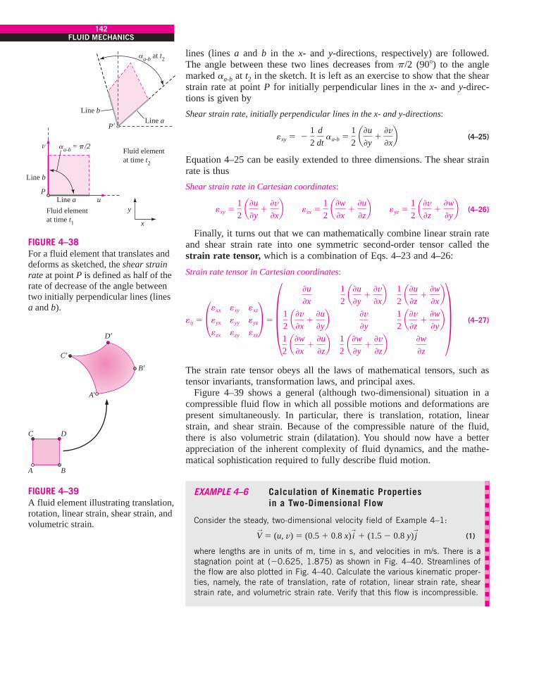
lines (lines a and b in the x- and y-directions, respectively) are followed.The angle between these two lines decreases from p/2 (90*) to the anglemarked aa-b at t2 in the sketch. It is left as an exercise to show that the shearstrain rate at point P for initially perpendicular lines in the x- and y-direc-tions is given by

Shear strain rate, initially perpendicular lines in the x- and y-directions:

(4–25)

Equation 4–25 can be easily extended to three dimensions. The shear strainrate is thus

Shear strain rate in Cartesian coordinates:

(4–26)

Finally, it turns out that we can mathematically combine linear strain rateand shear strain rate into one symmetric second-order tensor called thestrain rate tensor, which is a combination of Eqs. 4–23 and 4–26:

Strain rate tensor in Cartesian coordinates:

(4–27)

The strain rate tensor obeys all the laws of mathematical tensors, such astensor invariants, transformation laws, and principal axes.

Figure 4–39 shows a general (although two-dimensional) situation in acompressible fluid flow in which all possible motions and deformations arepresent simultaneously. In particular, there is translation, rotation, linearstrain, and shear strain. Because of the compressible nature of the fluid,there is also volumetric strain (dilatation). You should now have a betterappreciation of the inherent complexity of fluid dynamics, and the mathe-matical sophistication required to fully describe fluid motion.

EXAMPLE 4–6 Calculation of Kinematic Properties in a Two-Dimensional Flow

Consider the steady, two-dimensional velocity field of Example 4–1:

(1)

where lengths are in units of m, time in s, and velocities in m/s. There is astagnation point at ("0.625, 1.875) as shown in Fig. 4–40. Streamlines ofthe flow are also plotted in Fig. 4–40. Calculate the various kinematic proper-ties, namely, the rate of translation, rate of rotation, linear strain rate, shearstrain rate, and volumetric strain rate. Verify that this flow is incompressible.

V!

! (u, v) ! (0.5 # 0.8 x) i!

# (1.5 " 0.8 y) j!

eij ! £exx

eyx

ezx

exy

eyy

ezy

exz

eyz

ezz

" ! ¶ $u$x

12 a$v

$x#

$u$yb

12 a$w

$x#

$u$zb

12 a$u

$y#

$v$xb

$v$y

12 a$w

$y#

$v$zb

12 a$u

$z#

$w$xb

12 a$v

$z#

$w$yb

$w$z

#exy !

12 a$u

$y#

$v$xb ezx !

12 a$w

$x#

$u$zb eyz !

12 a$v

$z#

$w$yb

exy ! "12 ddt

aa-b !12 a$u

$y#

$v$xb

142FLUID MECHANICS

aa-b at t2

Line a

Line a u

v

y

x

Fluid elementat time t2

Fluid elementat time t1

Line b

Line b

P+

P

aa-b = p/2

FIGURE 4–38For a fluid element that translates anddeforms as sketched, the shear strainrate at point P is defined as half of therate of decrease of the angle betweentwo initially perpendicular lines (linesa and b).

C D

A B

C+

D+

A+

B+

FIGURE 4–39A fluid element illustrating translation,rotation, linear strain, shear strain, andvolumetric strain.

cen72367_ch04.qxd 12/1/04 6:19 PM Page 142

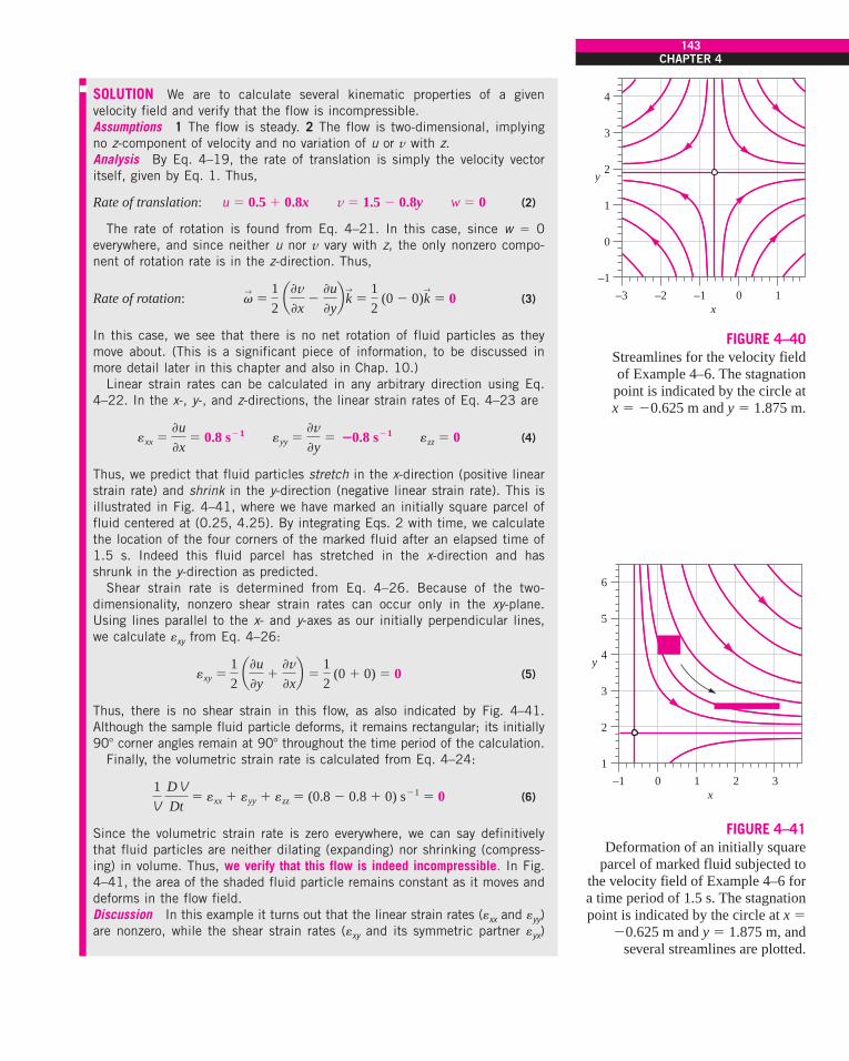
SOLUTION We are to calculate several kinematic properties of a givenvelocity field and verify that the flow is incompressible.Assumptions 1 The flow is steady. 2 The flow is two-dimensional, implyingno z-component of velocity and no variation of u or v with z.Analysis By Eq. 4–19, the rate of translation is simply the velocity vectoritself, given by Eq. 1. Thus,

Rate of translation: (2)

The rate of rotation is found from Eq. 4–21. In this case, since w ! 0everywhere, and since neither u nor v vary with z, the only nonzero compo-nent of rotation rate is in the z-direction. Thus,

Rate of rotation: (3)

In this case, we see that there is no net rotation of fluid particles as theymove about. (This is a significant piece of information, to be discussed inmore detail later in this chapter and also in Chap. 10.)

Linear strain rates can be calculated in any arbitrary direction using Eq.4–22. In the x-, y-, and z-directions, the linear strain rates of Eq. 4–23 are

(4)

Thus, we predict that fluid particles stretch in the x-direction (positive linearstrain rate) and shrink in the y-direction (negative linear strain rate). This isillustrated in Fig. 4–41, where we have marked an initially square parcel offluid centered at (0.25, 4.25). By integrating Eqs. 2 with time, we calculatethe location of the four corners of the marked fluid after an elapsed time of1.5 s. Indeed this fluid parcel has stretched in the x-direction and hasshrunk in the y-direction as predicted.

Shear strain rate is determined from Eq. 4–26. Because of the two-dimensionality, nonzero shear strain rates can occur only in the xy-plane.Using lines parallel to the x- and y-axes as our initially perpendicular lines,we calculate exy from Eq. 4–26:

(5)

Thus, there is no shear strain in this flow, as also indicated by Fig. 4–41.Although the sample fluid particle deforms, it remains rectangular; its initially90* corner angles remain at 90* throughout the time period of the calculation.

Finally, the volumetric strain rate is calculated from Eq. 4–24:

(6)

Since the volumetric strain rate is zero everywhere, we can say definitivelythat fluid particles are neither dilating (expanding) nor shrinking (compress-ing) in volume. Thus, we verify that this flow is indeed incompressible. In Fig.4–41, the area of the shaded fluid particle remains constant as it moves anddeforms in the flow field.Discussion In this example it turns out that the linear strain rates (exx and eyy)are nonzero, while the shear strain rates (exy and its symmetric partner eyx)

1V

D VDt

! exx # eyy # ezz ! (0.8 " 0.8 # 0) s"1 ! 0

exy !12 a$u

$y#

$v$xb !

12 (0 # 0) ! 0

exx !$u$x

! 0.8 s"1 eyy !$v$y

! "0.8 s"1 ezz ! 0

v!

!12 a$v

$x"

$u$ybk

!!

12 (0 " 0)k

!! 0

u ! 0.5 # 0.8x v ! 1.5 " 0.8y w ! 0

143CHAPTER 4

4

3

2y

1

0

–1–3 –2 –1 0

x1

FIGURE 4–40Streamlines for the velocity field of Example 4–6. The stagnation

point is indicated by the circle at x ! "0.625 m and y ! 1.875 m.

6

5

4y

3

2

1–1 0 1 2

x3

FIGURE 4–41Deformation of an initially square

parcel of marked fluid subjected to the velocity field of Example 4–6 for a time period of 1.5 s. The stagnationpoint is indicated by the circle at x !

"0.625 m and y ! 1.875 m, andseveral streamlines are plotted.

cen72367_ch04.qxd 12/1/04 6:19 PM Page 143

are zero. This means that the x- and y-axes of this flow field are the principalaxes. The (two-dimensional) strain rate tensor in this orientation is thus

(7)

If we were to rotate the axes by some arbitrary angle, the new axes would notbe principal axes, and all four elements of the strain rate tensor would benonzero. You may recall rotating axes in your engineering mechanics classesthrough use of Mohr’s circles to determine principal axes, maximum shearstrains, etc. Similar analyses can be performed in fluid mechanics.

Vorticity and RotationalityWe have already defined the rate of rotation vector of a fluid element (seeEq. 4–21). A closely related kinematic property is of great importance to theanalysis of fluid flows. Namely, the vorticity vector is defined mathemati-cally as the curl of the velocity vector V

!,

Vorticity vector: (4–28)

Physically, you can tell the direction of the vorticity vector by using theright-hand rule for cross product (Fig. 4–42). The symbol z used for vortic-ity is the Greek letter zeta. You should note that this symbol for vorticity isnot universal among fluid mechanics textbooks; some authors use the Greekletter omega (v) while still others use uppercase omega (-). In this book, v

!

is used to denote the rate of rotation vector (angular velocity vector) of afluid element. It turns out that the rate of rotation vector is equal to half ofthe vorticity vector,

Rate of rotation vector: (4–29)

Thus, vorticity is a measure of rotation of a fluid particle. Specifically,

Vorticity is equal to twice the angular velocity of a fluid particle (Fig. 4–43).

If the vorticity at a point in a flow field is nonzero, the fluid particle thathappens to occupy that point in space is rotating; the flow in that region iscalled rotational. Likewise, if the vorticity in a region of the flow is zero(or negligibly small), fluid particles there are not rotating; the flow in thatregion is called irrotational. Physically, fluid particles in a rotational regionof flow rotate end over end as they move along in the flow. For example,fluid particles within the viscous boundary layer near a solid wall are rota-tional (and thus have nonzero vorticity), while fluid particles outside theboundary layer are irrotational (and their vorticity is zero). Both of thesecases are illustrated in Fig. 4–44.

Rotation of fluid elements is associated with wakes, boundary layers, flowthrough turbomachinery (fans, turbines, compressors, etc.), and flow withheat transfer. The vorticity of a fluid element cannot change except throughthe action of viscosity, nonuniform heating (temperature gradients), or othernonuniform phenomena. Thus if a flow originates in an irrotational region,it remains irrotational until some nonuniform process alters it. For example,

v!

!12 §

!. V

!!

12 curl(V

!) !z!

2

z!

! §!

. V!

! curl(V!

)

eij ! aexx

eyx

exy

eyyb ! a0.8

00

"0.8b s"1

144FLUID MECHANICS

C = A . B

A

B

! !!

!

!

FIGURE 4–42The direction of a vector cross productis determined by the right-hand rule.

z

v!

!

FIGURE 4–43The vorticity vector is equal to twicethe angular velocity vector of arotating fluid particle.

cen72367_ch04.qxd 12/1/04 6:19 PM Page 144

air entering an inlet from quiescent (still) surroundings is irrotational andremains so unless it encounters an object in its path or is subjected tononuniform heating. If a region of flow can be approximated as irrotational,the equations of motion are greatly simplified, as you will see in Chap. 10.

In Cartesian coordinates, (i!

, j!

, k!

), (x, y, z), and (u, v, w), Eq. 4–28 can beexpanded as follows:

Vorticity vector in Cartesian coordinates:

(4–30)

If the flow is two-dimensional in the xy-plane, the z-component of velocity(w) is zero and neither u nor v varies with z. Thus the first two componentsof Eq. 4–30 are identically zero and the vorticity reduces to

Two-dimensional flow in Cartesian coordinates:

(4–31)

Note that if a flow is two-dimensional in the xy-plane, the vorticity vectormust point in either the z- or "z-direction (Fig. 4–45).

EXAMPLE 4–7 Vorticity Contours in a Two-Dimensional Flow

Consider the CFD calculation of two-dimensional free-stream flow impingingon a block of rectangular cross section, as shown in Figs. 4–32 and 4–33.Plot vorticity contours and discuss.

SOLUTION We are to calculate the vorticity field for a given velocity fieldproduced by CFD and then generate a contour plot of vorticity.Analysis Since the flow is two-dimensional, the only nonzero component ofvorticity is in the z-direction, normal to the page in Figs. 4–32 and 4–33. Acontour plot of the z-component of vorticity for this flow field is shown in Fig.4–46. The dark region near the upper-left corner of the block indicates largenegative values of vorticity, implying clockwise rotation of fluid particles inthat region. This is due to the large velocity gradients encountered in this por-tion of the flow field; the boundary layer separates off the wall at the corner of

z!

! ¢$v$x

"$u$y!k

!

z!

! a$w$y

"$v$zb i

!# a$u

$z"

$w$xb j

!# a$v

$x"

$u$ybk

!

145CHAPTER 4

Fluid particles not rotating

Velocity profileIrrotational outer flow region

Rotational boundary layer region

Fluid particles rotatingWall

FIGURE 4–44The difference between rotational and

irrotational flow: fluid elements in arotational region of the flow rotate, but

those in an irrotational region of theflow do not.

yz

x

z!

FIGURE 4–45For a two-dimensional flow in the

xy-plane, the vorticity vector alwayspoints in the z- or "z-direction. In

this illustration, the flag-shaped fluidparticle rotates in the counterclockwise

direction as it moves in the xy-plane;its vorticity points in the positive

z-direction as shown.

Block

Symmetry plane

FLOWFLOW

FIGURE 4–46Contour plot of the vorticity field zz

due to flow impinging on a block,as produced by CFD calculations;

only the upper half is shown due tosymmetry. Dark regions representlarge negative vorticity, and light

regions represent large positivevorticity.

cen72367_ch04.qxd 12/1/04 6:19 PM Page 145

146FLUID MECHANICS

4

3

y2

1

00 1 2 3

x4

"t = 0

"t = 0.25 s

"t = 0.50 s

FIGURE 4–47Deformation of an initially squarefluid parcel subjected to the velocityfield of Example 4–8 for a time periodof 0.25 s and 0.50 s. Several streamlinesare also plotted in the first quadrant. Itis clear that this flow is rotational.

the body and forms a thin shear layer across which the velocity changesrapidly. The concentration of vorticity in the shear layer diminishes as vorticitydiffuses downstream. The small lightly shaded region near the top right cornerof the block represents a region of positive vorticity (counterclockwise rota-tion)—a secondary flow pattern caused by the flow separation.Discussion We expect the magnitude of vorticity to be highest in regionswhere spatial derivatives of velocity are high (see Eq. 4–30). Close examina-tion reveals that the dark region in Fig. 4–46 does indeed correspond tolarge velocity gradients in Fig. 4–32. Keep in mind that the vorticity field ofFig. 4–46 is time-averaged. The instantaneous flow field is in reality turbu-lent and unsteady, and vortices are shed from the bluff body.

EXAMPLE 4–8 Determination of Rotationality in a Two-Dimensional Flow

Consider the following steady, incompressible, two-dimensional velocity field:

(1)

Is this flow rotational or irrotational? Sketch some streamlines in the firstquadrant and discuss.

SOLUTION We are to determine whether a flow with a given velocity field isrotational or irrotational, and we are to draw some streamlines in the firstquadrant.Analysis Since the flow is two-dimensional, Eq. 4–31 is valid. Thus,

Vorticity: (2)

Since the vorticity is nonzero, this flow is rotational. In Fig. 4–47 we plotseveral streamlines of the flow in the first quadrant; we see that fluid movesdownward and to the right. The translation and deformation of a fluid parcelis also shown: at 't ! 0, the fluid parcel is square, at 't ! 0.25 s, it hasmoved and deformed, and at 't ! 0.50 s, the parcel has moved farther andis further deformed. In particular, the right-most portion of the fluid parcelmoves faster to the right and faster downward compared to the left-most por-tion, stretching the parcel in the x-direction and squashing it in the verticaldirection. It is clear that there is also a net clockwise rotation of the fluidparcel, which agrees with the result of Eq. 2.Discussion From Eq. 4–29, individual fluid particles rotate at an angularvelocity equal to v

!! "yk

!, half of the vorticity vector. Since v

!is not con-

stant, this flow is not solid-body rotation. Rather, v!

is a linear function of y.Further analysis reveals that this flow field is incompressible; the shadedareas representing the fluid parcel in Fig. 4–47 remain constant at all threeinstants in time.

In cylindrical coordinates, (e!r, e!u, e!z), (r, u, z), and (ur, uu, uz), Eq. 4–28can be expanded asVorticity vector in cylindrical coordinates:

(4–32)z!

! a1r $uz

$u"

$uu$zbe

!r # a$ur

$z"

$uz

$rbe

!u #

1ra$(ruu)

$r"

$ur

$ube

!z

z!

! ¢$v$x

"$u$y!k

!! ("2y " 0)k

!! "2yk

!

V!

! (u, v) ! x 2 i!

# ("2xy " 1) j!

cen72367_ch04.qxd 12/1/04 6:19 PM Page 146

For two-dimensional flow in the ru-plane, Eq. 4–32 reduces to

Two-dimensional flow in cylindrical coordinates:

(4–33)

where k!

is used as the unit vector in the z-direction in place of e!z. Note thatif a flow is two-dimensional in the ru-plane, the vorticity vector must pointin either the z- or "z-direction (Fig. 4–48).

Comparison of Two Circular FlowsNot all flows with circular streamlines are rotational. To illustrate this point,we consider two incompressible, steady, two-dimensional flows, both ofwhich have circular streamlines in the ru-plane:

Flow A—solid-body rotation: (4–34)

Flow B—line vortex: (4–35)

where v and K are constants. (Alert readers will note that uu in Eq. 4–35 isinfinite at r ! 0, which is of course physically impossible; we ignore theregion close to the origin to avoid this problem.) Since the radial componentof velocity is zero in both cases, the streamlines are circles about the origin.The velocity profiles for the two flows, along with their streamlines, aresketched in Fig. 4–49. We now calculate and compare the vorticity field foreach of these flows, using Eq. 4–33.

Flow A—solid-body rotation: (4–36)

Flow B—line vortex: (4–37)

Not surprisingly, the vorticity for solid-body rotation is nonzero. In fact, it isa constant of magnitude twice the angular velocity and pointing in the samedirection. (This agrees with Eq. 4–29.) Flow A is rotational. Physically, thismeans that individual fluid particles rotate as they revolve around the origin(Fig. 4–49a). By contrast, the vorticity of the line vortex is identically zeroeverywhere (except right at the origin, which is a mathematical singularity).Flow B is irrotational. Physically, fluid particles do not rotate as theyrevolve in circles about the origin (Fig. 4–49b).

A simple analogy can be made between flow A and a merry-go-round orroundabout, and flow B and a Ferris wheel (Fig. 4–50). As children revolvearound a roundabout, they also rotate at the same angular velocity as that ofthe ride itself. This is analogous to a rotational flow. In contrast, children ona Ferris wheel always remain oriented in an upright position as they traceout their circular path. This is analogous to an irrotational flow.

z!

!1ra$(K)

$r" 0bk

!! 0

z!

!1ra$(vr 2)

$r" 0bk

!! 2vk

!

ur ! 0 and uu !Kr

ur ! 0 and uu ! vr

z!

!1ra$(ruu)

$r"

$ur

$ubk

!

147CHAPTER 4

y

z

x

ru

z!

FIGURE 4–48For a two-dimensional flow in the

ru-plane, the vorticity vector alwayspoints in the z (or "z) direction. In

this illustration, the flag-shaped fluidparticle rotates in the clockwise

direction as it moves in the ru-plane;its vorticity points in the "z-direction

as shown.

Flow A uu

uu = vr

r

(a)

Flow B uu

r

(b)

uu = rK

FIGURE 4–49Streamlines and velocity profiles for

(a) flow A, solid-body rotation and(b) flow B, a line vortex. Flow A isrotational, but flow B is irrotational

everywhere except at the origin.

cen72367_ch04.qxd 12/1/04 6:19 PM Page 147

EXAMPLE 4–9 Determination of Rotationality of a Line Sink

A simple two-dimensional velocity field called a line sink is often used tosimulate fluid being sucked into a line along the z-axis. Suppose the volumeflow rate per unit length along the z-axis, V

./L, is known, where V

.is a nega-

tive quantity. In two dimensions in the ru-plane,

Line sink: (1)

Draw several streamlines of the flow and calculate the vorticity. Is this flowrotational or irrotational?

SOLUTION Streamlines of the given flow field are to be sketched and therotationality of the flow is to be determined.Analysis Since there is only radial flow and no tangential flow, we knowimmediately that all streamlines must be rays into the origin. Several stream-lines are sketched in Fig. 4–51. The vorticity is calculated from Eq. 4–33:

(2)

Since the vorticity vector is everywhere zero, this flow field is irrotational.Discussion Many practical flow fields involving suction, such as flow intoinlets and hoods, can be approximated quite accurately by assuming irrota-tional flow (Heinsohn and Cimbala, 2003).

4–5 ! THE REYNOLDS TRANSPORT THEOREMIn thermodynamics and solid mechanics we often work with a system (alsocalled a closed system), defined as a quantity of matter of fixed identity. Influid dynamics, it is more common to work with a control volume (also

z!

!1ra$(ruu)

$r"

$

$u urb k

!!

1ra0 "

$

$u a V#

2pL 1rbb k

!! 0

ur !V#

2pL 1r and uu ! 0

148FLUID MECHANICS

FIGURE 4–50A simple analogy: (a) rotational circular flow is analogous to a roundabout,while (b) irrotational circular flow is analogous to a Ferris wheel.© Robb Gregg/PhotoEdit

y

x

Streamlines

u

r

FIGURE 4–51Streamlines in the ru-plane for thecase of a line sink.

(a) (b)

cen72367_ch04.qxd 12/1/04 6:19 PM Page 148

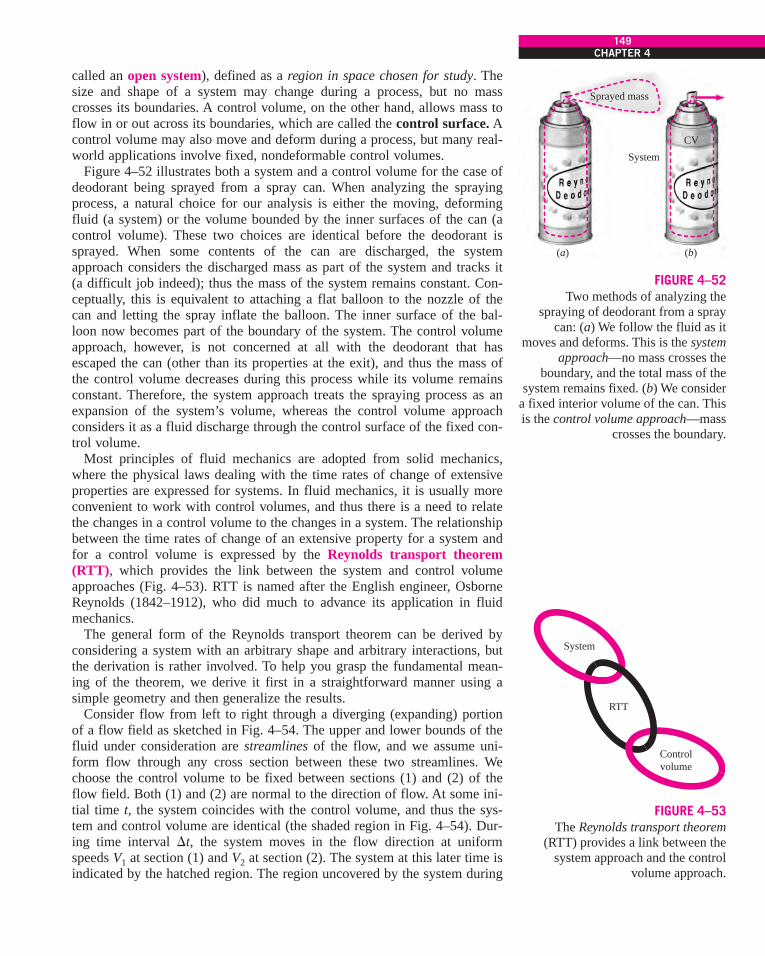
called an open system), defined as a region in space chosen for study. Thesize and shape of a system may change during a process, but no masscrosses its boundaries. A control volume, on the other hand, allows mass toflow in or out across its boundaries, which are called the control surface. Acontrol volume may also move and deform during a process, but many real-world applications involve fixed, nondeformable control volumes.

Figure 4–52 illustrates both a system and a control volume for the case ofdeodorant being sprayed from a spray can. When analyzing the sprayingprocess, a natural choice for our analysis is either the moving, deformingfluid (a system) or the volume bounded by the inner surfaces of the can (acontrol volume). These two choices are identical before the deodorant issprayed. When some contents of the can are discharged, the systemapproach considers the discharged mass as part of the system and tracks it(a difficult job indeed); thus the mass of the system remains constant. Con-ceptually, this is equivalent to attaching a flat balloon to the nozzle of thecan and letting the spray inflate the balloon. The inner surface of the bal-loon now becomes part of the boundary of the system. The control volumeapproach, however, is not concerned at all with the deodorant that hasescaped the can (other than its properties at the exit), and thus the mass ofthe control volume decreases during this process while its volume remainsconstant. Therefore, the system approach treats the spraying process as anexpansion of the system’s volume, whereas the control volume approachconsiders it as a fluid discharge through the control surface of the fixed con-trol volume.

Most principles of fluid mechanics are adopted from solid mechanics,where the physical laws dealing with the time rates of change of extensiveproperties are expressed for systems. In fluid mechanics, it is usually moreconvenient to work with control volumes, and thus there is a need to relatethe changes in a control volume to the changes in a system. The relationshipbetween the time rates of change of an extensive property for a system andfor a control volume is expressed by the Reynolds transport theorem(RTT), which provides the link between the system and control volumeapproaches (Fig. 4–53). RTT is named after the English engineer, OsborneReynolds (1842–1912), who did much to advance its application in fluidmechanics.

The general form of the Reynolds transport theorem can be derived byconsidering a system with an arbitrary shape and arbitrary interactions, butthe derivation is rather involved. To help you grasp the fundamental mean-ing of the theorem, we derive it first in a straightforward manner using asimple geometry and then generalize the results.

Consider flow from left to right through a diverging (expanding) portionof a flow field as sketched in Fig. 4–54. The upper and lower bounds of thefluid under consideration are streamlines of the flow, and we assume uni-form flow through any cross section between these two streamlines. Wechoose the control volume to be fixed between sections (1) and (2) of theflow field. Both (1) and (2) are normal to the direction of flow. At some ini-tial time t, the system coincides with the control volume, and thus the sys-tem and control volume are identical (the shaded region in Fig. 4–54). Dur-ing time interval 't, the system moves in the flow direction at uniformspeeds V1 at section (1) and V2 at section (2). The system at this later time isindicated by the hatched region. The region uncovered by the system during

149CHAPTER 4

(a)

Sprayed mass

(b)

System

CV

FIGURE 4–52Two methods of analyzing the

spraying of deodorant from a spraycan: (a) We follow the fluid as it

moves and deforms. This is the systemapproach—no mass crosses the

boundary, and the total mass of thesystem remains fixed. (b) We consider

a fixed interior volume of the can. Thisis the control volume approach—mass

crosses the boundary.

Controlvolume

RTT

System

FIGURE 4–53The Reynolds transport theorem

(RTT) provides a link between thesystem approach and the control

volume approach.

cen72367_ch04.qxd 12/1/04 6:19 PM Page 149

this motion is designated as section I (part of the CV), and the new regioncovered by the system is designated as section II (not part of the CV).Therefore, at time t # 't, the system consists of the same fluid, but it occu-pies the region CV " I # II. The control volume is fixed in space, and thusit remains as the shaded region marked CV at all times.

Let B represent any extensive property (such as mass, energy, or momen-tum), and let b ! B/m represent the corresponding intensive property. Not-ing that extensive properties are additive, the extensive property B of thesystem at times t and t # 't can be expressed as

Subtracting the first equation from the second one and dividing by 't gives

Taking the limit as 't ! 0, and using the definition of derivative, we get

(4–38)

or

since

and

where A1 and A2 are the cross-sectional areas at locations 1 and 2. Equation4–38 states that the time rate of change of the property B of the system isequal to the time rate of change of B of the control volume plus the net fluxof B out of the control volume by mass crossing the control surface. This isthe desired relation since it relates the change of a property of a system tothe change of that property for a control volume. Note that Eq. 4–38 appliesat any instant in time, where it is assumed that the system and the controlvolume occupy the same space at that particular instant in time.

The influx B.in and outflux B

.out of the property B in this case are easy to

determine since there is only one inlet and one outlet, and the velocities arenormal to the surfaces at sections (1) and (2). In general, however, we mayhave several inlet and outlet ports, and the velocity may not be normal tothe control surface at the point of entry. Also, the velocity may not be uni-form. To generalize the process, we consider a differential surface area dAon the control surface and denote its unit outer normal by n!. The flow rate

B#

out ! B#

II ! lim't!0

BII, t#'t

't! lim

't!0 b2r2V2 't A2

't! b2r2V2 A2

B#

in ! B#

I ! lim't!0

BI, t#'t

't! lim

't!0 b1r1V1 't A1

't! b1r1V1 A1

BII, t#'t ! b2mII, t#'t ! b2r2V II, t#'t ! b2r2V2 't A2

BI, t#'t ! b1mI, t#'t ! b1r1V I, t#'t ! b1r1V1 't A1

dBsys

dt!

dBCV

dt" b1r1V1A1 # b2r2V2A2

dBsys

dt!

dBCV

dt" B#

in # B#

out

Bsys, t#'t " Bsys, t

't!

BCV, t#'t " BCV, t

't"

BI, t#'t

't#

B/, t#'t

't

Bsys, t#'t ! BCV, t#'t " BI, t#'t # BII, t#'t

Bsys, t ! BCV, t (the system and CV concide at time t)

150FLUID MECHANICS

V2

II

Control volume at time t + "t (CV remains fixed in time)

At time t: Sys = CVAt time t + t: Sys = CV ) I + II

System (material volume) and control volume at time t (shaded region)

System at time t + "t (hatched region)

Outflow during "t

Inflow during "t

I

(1)

(2)

V1

"

FIGURE 4–54A moving system (hatched region) anda fixed control volume (shaded region)in a diverging portion of a flow field attimes t and t # 't. The upper and lowerbounds are streamlines of the flow.

cen72367_ch04.qxd 12/1/04 6:19 PM Page 150

of property b through dA is rbV!

· n! dA since the dot product V!

· n! gives thenormal component of the velocity. Then the net rate of outflow through theentire control surface is determined by integration to be (Fig. 4–55)

(4–39)

An important aspect of this relation is that it automatically subtracts theinflow from the outflow, as explained next. The dot product of the velocityvector at a point on the control surface and the outer normal at that point is

, where u is the angle between the velocityvector and the outer normal, as shown in Fig. 4–56. For u ) 90*, we havecos u ( 0 and thus V

!· n

!( 0 for outflow of mass from the control volume,

and for u ( 90*, we have cos u ) 0 and thus V!

· n!

) 0 for inflow of massinto the control volume. Therefore, the differential quantity rbV

!· n

!dA is

positive for mass flowing out of the control volume, and negative for massflowing into the control volume, and its integral over the entire control sur-face gives the rate of net outflow of the property B by mass.

The properties within the control volume may vary with position, in gen-eral. In such a case, the total amount of property B within the control vol-ume must be determined by integration:

(4–40)

The term dBCV/dt in Eq. 4–38 is thus equal to , and represents

the time rate of change of the property B content of the control volume. Apositive value for dBCV/dt indicates an increase in the B content, and a neg-ative value indicates a decrease. Substituting Eqs. 4–39 and 4–40 into Eq.4–38 yields the Reynolds transport theorem, also known as the system-to-control-volume transformation for a fixed control volume:

RTT, fixed CV: (4–41)

Since the control volume is not moving or deforming with time, the timederivative on the right-hand side can be moved inside the integral, since thedomain of integration does not change with time. (In other words, it is irrel-evant whether we differentiate or integrate first.) But the time derivative inthat case must be expressed as a partial derivative ($/$t) since density andthe quantity b may depend on the position within the control volume. Thus,an alternate form of the Reynolds transport theorem for a fixed control vol-ume is

Alternate RTT, fixed CV: (4–42)

Equation 4–41 was derived for a fixed control volume. However, manypractical systems such as turbine and propeller blades involve nonfixed con-trol volumes. Fortunately, Eq. 4–41 is also valid for moving and/or deform-ing control volumes provided that the absolute fluid velocity V

!in the last

term is replaced by the relative velocity V!

r ,

dBsys

dt! #

CV

$

$t (rb) d V # #

CS

rbV!

& n! dA

dBsys

dt!

ddt

#CV

rb dV # #CS

rbV!

& n! dA

ddt

#CV

rb dV

BCV ! #CV

rb d V

V!

& n! ! $V!

$$n!$ cos u ! $V!

$ cos u

B#

net ! B#

out " B#

in ! #CS

rbV!

& n! dA (inflow if negative)

151CHAPTER 4

Bnet = Bout – Bin = #CS

rbV & n dA· · ·

Control volume

nMass

entering

outwardnormal

Massleaving

Massleaving

! !

!

n!

n!

n!

n =!

FIGURE 4–55The integral of brV

!& n! dA over the

control surface gives the net amount of the property B flowing out of the

control volume (into the controlvolume if it is negative) per unit time.

If u < 90°, then cos u > 0 (outflow).If u > 90°, then cos u < 0 (inflow).If u = 90°, then cos u = 0 (no flow).

n

Outflow:u < 90°

dAn

Inflow:u > 90°

dA

& n = | || n | cos u = V cos u

!

V!

! !

V

V V

uu

!!

!!

FIGURE 4–56Outflow and inflow of mass across the

differential area of a control surface.

cen72367_ch04.qxd 12/1/04 6:20 PM Page 151

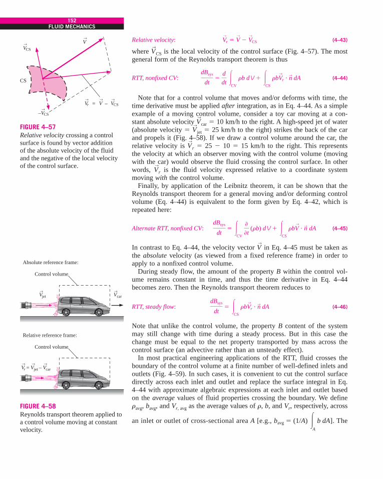
Relative velocity: (4–43)

where V!

CS is the local velocity of the control surface (Fig. 4–57). The mostgeneral form of the Reynolds transport theorem is thus

RTT, nonfixed CV: (4–44)

Note that for a control volume that moves and/or deforms with time, thetime derivative must be applied after integration, as in Eq. 4–44. As a simpleexample of a moving control volume, consider a toy car moving at a con-stant absolute velocity V

!

car ! 10 km/h to the right. A high-speed jet of water(absolute velocity ! V

!

jet ! 25 km/h to the right) strikes the back of the carand propels it (Fig. 4–58). If we draw a control volume around the car, therelative velocity is V

!

r ! 25 " 10 ! 15 km/h to the right. This representsthe velocity at which an observer moving with the control volume (movingwith the car) would observe the fluid crossing the control surface. In otherwords, V

!

r is the fluid velocity expressed relative to a coordinate systemmoving with the control volume.

Finally, by application of the Leibnitz theorem, it can be shown that theReynolds transport theorem for a general moving and/or deforming controlvolume (Eq. 4–44) is equivalent to the form given by Eq. 4–42, which isrepeated here:

Alternate RTT, nonfixed CV: (4–45)

In contrast to Eq. 4–44, the velocity vector V!

in Eq. 4–45 must be taken asthe absolute velocity (as viewed from a fixed reference frame) in order toapply to a nonfixed control volume.

During steady flow, the amount of the property B within the control vol-ume remains constant in time, and thus the time derivative in Eq. 4–44becomes zero. Then the Reynolds transport theorem reduces to

RTT, steady flow: (4–46)

Note that unlike the control volume, the property B content of the systemmay still change with time during a steady process. But in this case thechange must be equal to the net property transported by mass across thecontrol surface (an advective rather than an unsteady effect).

In most practical engineering applications of the RTT, fluid crosses theboundary of the control volume at a finite number of well-defined inlets andoutlets (Fig. 4–59). In such cases, it is convenient to cut the control surfacedirectly across each inlet and outlet and replace the surface integral in Eq.4–44 with approximate algebraic expressions at each inlet and outlet basedon the average values of fluid properties crossing the boundary. We defineravg, bavg, and Vr, avg as the average values of r, b, and Vr, respectively, across

an inlet or outlet of cross-sectional area A [e.g., ]. The bavg ! (10A) #A

b dA

dBsys

dt! #

CS

rbV!

r & n! dA

dBsys

dt! #

CV

$

$t (rb) dV # #

CS

rbV!

& n! dA

dBsys

dt!

ddt

#CV

rb dV # #CS

rbV!

r & n! dA

V!

r ! V!

" V!

CS

152FLUID MECHANICS

CS

= –r

–

!CSV

!CSV

!CS

!V

!VV

!V

FIGURE 4–57Relative velocity crossing a controlsurface is found by vector addition of the absolute velocity of the fluidand the negative of the local velocityof the control surface.

Control volume

Absolute reference frame:

Vjet Vcar

Control volume

Relative reference frame:

Vr = Vjet – Vcar

! !

!! !

FIGURE 4–58Reynolds transport theorem applied toa control volume moving at constantvelocity.

cen72367_ch04.qxd 12/1/04 6:20 PM Page 152

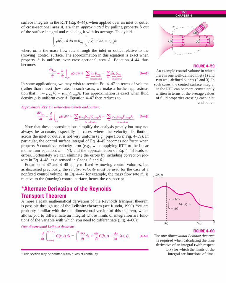
surface integrals in the RTT (Eq. 4–44), when applied over an inlet or outletof cross-sectional area A, are then approximated by pulling property b outof the surface integral and replacing it with its average. This yields

where m.r is the mass flow rate through the inlet or outlet relative to the(moving) control surface. The approximation in this equation is exact whenproperty b is uniform over cross-sectional area A. Equation 4–44 thusbecomes

(4–47)

In some applications, we may wish to rewrite Eq. 4–47 in terms of volume(rather than mass) flow rate. In such cases, we make a further approxima-tion that . This approximation is exact when fluiddensity r is uniform over A. Equation 4–47 then reduces to

Approximate RTT for well-defined inlets and outlets:

(4–48)

Note that these approximations simplify the analysis greatly but may notalways be accurate, especially in cases where the velocity distributionacross the inlet or outlet is not very uniform (e.g., pipe flows; Fig. 4–59). Inparticular, the control surface integral of Eq. 4–45 becomes nonlinear whenproperty b contains a velocity term (e.g., when applying RTT to the linearmomentum equation, b ! V

!), and the approximation of Eq. 4–48 leads to

errors. Fortunately we can eliminate the errors by including correction fac-tors in Eq. 4–48, as discussed in Chaps. 5 and 6.

Equations 4–47 and 4–48 apply to fixed or moving control volumes, butas discussed previously, the relative velocity must be used for the case of anonfixed control volume. In Eq. 4–47 for example, the mass flow rate m.r isrelative to the (moving) control surface, hence the r subscript.

*Alternate Derivation of the Reynolds Transport TheoremA more elegant mathematical derivation of the Reynolds transport theoremis possible through use of the Leibnitz theorem (see Kundu, 1990). You areprobably familiar with the one-dimensional version of this theorem, whichallows you to differentiate an integral whose limits of integration are func-tions of the variable with which you need to differentiate (Fig. 4–60):

One-dimensional Leibnitz theorem:

(4–49)ddt

#x!b(t)

x!a(t)

G(x, t) dx ! #b

a

$G$t

dx #dbdt

G(b, t) "dadt

G(a, t)

dBsys

dt!

ddt

#CV

rb dV # aoutravgbavgVr, avg A " a

inravgbavgVr,avg A

m#

r % ravgV#r ! ravgVr, avg A

dBsys

dt!

ddt

#CV

rb dV # aout

m#

r

bavg " ain

m#

r bavg

#A

rbV!

r & n! dA " bavg #A

rV!

r & n! dA ! bavgm#

r

153CHAPTER 4

CV

1 2

3

FIGURE 4–59An example control volume in whichthere is one well-defined inlet (1) andtwo well-defined outlets (2 and 3). In

such cases, the control surface integralin the RTT can be more convenientlywritten in terms of the average valuesof fluid properties crossing each inlet

and outlet.

for each outlet for each inlet

$%&$%&

for each outlet for each inlet

$''%''& $''%''&

G(x, t)

xb(t)a(t)

x = b(t)

x = a(t)# G(x, t) dx

FIGURE 4–60The one-dimensional Leibnitz theorem

is required when calculating the timederivative of an integral (with respect

to x) for which the limits of theintegral are functions of time.* This section may be omitted without loss of continuity.

cen72367_ch04.qxd 12/1/04 6:20 PM Page 153

The Leibnitz theorem takes into account the change of limits a(t) and b(t)with respect to time, as well as the unsteady changes of integrand G(x, t)with time.

EXAMPLE 4–10 One-Dimensional Leibnitz Integration

Reduce the following expression as far as possible:

(1)

SOLUTION F(t) is to be evaluated from the given expression.Analysis We could try integrating first and then differentiating, but sinceEq. 1 is of the form of Eq. 4–49, we use the one-dimensional Leibnitz theo-rem. Here, G(x, t) ! e"x2 (G is not a function of time in this simple exam-ple). The limits of integration are a(t) ! 0 and b(t) ! Ct. Thus,

(2)

Discussion You are welcome to try to obtain the same solution without usingthe Leibnitz theorem.

In three dimensions, the Leibnitz theorem for a volume integral is

Three-dimensional Leibnitz theorem:

(4–50)

where V(t) is a moving and/or deforming volume (a function of time), A(t)is its surface (boundary), and V

!

A is the absolute velocity of this (moving)surface (Fig. 4–61). Equation 4–50 is valid for any volume, moving and/ordeforming arbitrarily in space and time. For consistency with the previousanalyses, we set integrand G to rb for application to fluid flow,

Three-dimensional Leibnitz theorem applied to fluid flow:

(4–51)

If we apply the Leibnitz theorem to the special case of a material volume(a system of fixed identity moving with the fluid flow), then V

!

A ! V!

every-where on the material surface since it moves with the fluid. Here V

!is the

local fluid velocity, and Eq. 4–51 becomes

Leibnitz theorem applied to a material volume:

(4–52)

Equation 4–52 is valid at any instant in time t. We define our control vol-ume such that at this time t, the control volume and the system occupy thesame space; in other words, they are coincident. At some later time t # 't,the system has moved and deformed with the flow, but the control volume

ddt

#V(t)

rb dV !dBsys

dt! #

V(t)

$

$t (rb) dV # #

A(t)

rbV!

& n! dA

ddt

#V(t)

rb dV ! #V(t)

$

$t (rb) dV # #

A(t)

rbV!

A & n! dA

ddt

#V(t)

G(x, y, z, t) dV ! #V(t)

$G$t

dV # #A(t)

GV!

A & n! dA

F(t) ! #b

a

$G$t

dx #dbdt

G(b, t) "dadt

G(a, t) ! F(t) ! Ce"C

2t 2

F(t) !ddt

#x!Ct

x!0

e"x2

dx

154FLUID MECHANICS

0 C e"b2 0

$%&F F F

A(t)

V(t)

G(x, y, z, t) d V

G(x, y, z, t)VA!

V(t)#

FIGURE 4–61The three-dimensional Leibnitztheorem is required when calculatingthe time derivative of a volumeintegral for which the volume itselfmoves and/or deforms with time. Itturns out that the three-dimensionalform of the Leibnitz theorem can beused in an alternative derivation of the Reynolds transport theorem.

cen72367_ch04.qxd 12/1/04 6:20 PM Page 154

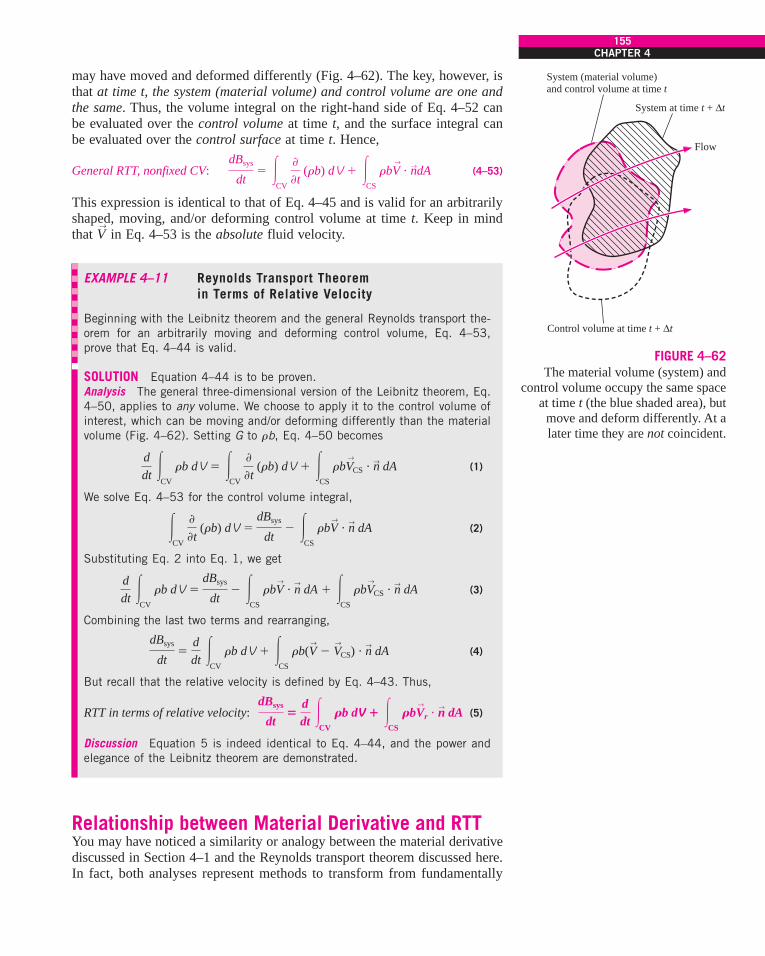
may have moved and deformed differently (Fig. 4–62). The key, however, isthat at time t, the system (material volume) and control volume are one andthe same. Thus, the volume integral on the right-hand side of Eq. 4–52 canbe evaluated over the control volume at time t, and the surface integral canbe evaluated over the control surface at time t. Hence,

General RTT, nonfixed CV: (4–53)

This expression is identical to that of Eq. 4–45 and is valid for an arbitrarilyshaped, moving, and/or deforming control volume at time t. Keep in mindthat V

!in Eq. 4–53 is the absolute fluid velocity.

EXAMPLE 4–11 Reynolds Transport Theorem in Terms of Relative Velocity

Beginning with the Leibnitz theorem and the general Reynolds transport the-orem for an arbitrarily moving and deforming control volume, Eq. 4–53,prove that Eq. 4–44 is valid.

SOLUTION Equation 4–44 is to be proven.Analysis The general three-dimensional version of the Leibnitz theorem, Eq.4–50, applies to any volume. We choose to apply it to the control volume ofinterest, which can be moving and/or deforming differently than the materialvolume (Fig. 4–62). Setting G to rb, Eq. 4–50 becomes

(1)

We solve Eq. 4–53 for the control volume integral,

(2)

Substituting Eq. 2 into Eq. 1, we get

(3)

Combining the last two terms and rearranging,

(4)

But recall that the relative velocity is defined by Eq. 4–43. Thus,

RTT in terms of relative velocity: (5)

Discussion Equation 5 is indeed identical to Eq. 4–44, and the power andelegance of the Leibnitz theorem are demonstrated.

Relationship between Material Derivative and RTTYou may have noticed a similarity or analogy between the material derivativediscussed in Section 4–1 and the Reynolds transport theorem discussed here.In fact, both analyses represent methods to transform from fundamentally

dBsys

dt!

ddt

#CV

Rb dV # #CS

RbV!

r & n! dA

dBsys

dt!

ddt

#CV

rb dV # #CS

rb(V!

" V!

CS) & n! dA

ddt

#CV

rb dV !dBsys

dt" #

CS

rbV!

& n! dA # #

CS

rbV!

CS & n! dA

#CV

$

$t (rb) dV !

dBsys

dt" #

CS

rbV!

& n! dA

ddt

#CV

rb dV ! #CV

$

$t (rb) dV # #

CS

rbV!

CS & n! dA

dBsys

dt! #

CV

$

$t (rb) dV # #

CS

rbV!

& n!dA

155CHAPTER 4

Flow

System (material volume)and control volume at time t

Control volume at time t + "t

System at time t + "t

FIGURE 4–62The material volume (system) and

control volume occupy the same spaceat time t (the blue shaded area), but

move and deform differently. At a later time they are not coincident.

cen72367_ch04.qxd 12/1/04 6:20 PM Page 155

Lagrangian concepts to Eulerian interpretations of those concepts. While theReynolds transport theorem deals with finite-size control volumes and thematerial derivative deals with infinitesimal fluid particles, the same funda-mental physical interpretation applies to both (Fig. 4–63). In fact, theReynolds transport theorem can be thought of as the integral counterpart ofthe material derivative. In either case, the total rate of change of some prop-erty following an identified portion of fluid consists of two parts: There is alocal or unsteady part that accounts for changes in the flow field with time(compare the first term on the right-hand side of Eq. 4-12 to that of Eq. 4-45). There is also an advective part that accounts for the movement of fluidfrom one region of the flow to another (compare the second term on theright-hand sides of Eqs. 4-12 and 4-45).

Just as the material derivative can be applied to any fluid property, scalaror vector, the Reynolds transport theorem can be applied to any scalar orvector property as well. In Chaps. 5 and 6, we apply the Reynolds transporttheorem to conservation of mass, energy, momentum, and angular momen-tum by choosing parameter B to be mass, energy, momentum, and angularmomentum, respectively. In this fashion we can easily convert from the fun-damental system conservation laws (Lagrangian viewpoint) to forms that arevalid and useful in a control volume analysis (Eulerian viewpoint).

156FLUID MECHANICS

Lagrangiandescription

Euleriandescription

Systemanalysis RTT

Controlvolumeanalysis

DDt

FIGURE 4–63The Reynolds transport theorem forfinite volumes (integral analysis) isanalogous to the material derivativefor infinitesimal volumes (differentialanalysis). In both cases, we transformfrom a Lagrangian or system viewpointto an Eulerian or control volumeviewpoint.

SUMMARY

Fluid kinematics is concerned with describing fluid motion,without necessarily analyzing the forces responsible for suchmotion. There are two fundamental descriptions of fluidmotion—Lagrangian and Eulerian. In a Lagrangian descrip-tion, we follow individual fluid particles or collections offluid particles, while in the Eulerian description, we define acontrol volume through which fluid flows in and out. Wetransform equations of motion from Lagrangian to Eulerianthrough use of the material derivative for infinitesimal fluidparticles and through use of the Reynolds transport theorem(RTT) for systems of finite volume. For some extensive prop-erty B or its corresponding intensive property b,

Material derivative:

General RTT, nonfixed CV:

In both equations, the total change of the property following afluid particle or following a system is composed of two parts:a local (unsteady) part and an advective (movement) part.

There are various ways to visualize and analyze flowfields—streamlines, streaklines, pathlines, timelines, surface

dBsys

dt! #

CV

$

$t (rb) dV # #

CS

rbV!

& n! dA

DbDt

!$b$t

# (V!

& §!

)b

imaging, shadowgraphy, schlieren imaging, profile plots, vec-tor plots, and contour plots. We define each of these and pro-vide examples in this chapter. In general unsteady flow,streamlines, streaklines, and pathlines differ, but in steadyflow, streamlines, streaklines, and pathlines are coincident.

Four fundamental rates of motion (deformation rates) arerequired to fully describe the kinematics of a fluid flow: veloc-ity (rate of translation), angular velocity (rate of rotation), lin-ear strain rate, and shear strain rate. Vorticity is a property offluid flows that indicates the rotationality of fluid particles.

Vorticity vector:

A region of flow is irrotational if the vorticity is zero in thatregion.

The concepts learned in this chapter are used repeatedlythroughout the rest of the book. We use the RTT to transformthe conservation laws from closed systems to control vol-umes in Chaps. 5 and 6, and again in Chap. 9 in the deriva-tion of the differential equations of fluid motion. The role ofvorticity and irrotationality is revisited in greater detail inChap. 10 where we show that the irrotationality approxima-tion leads to greatly reduced complexity in the solution offluid flows. Finally, we use various types of flow visualiza-tion and data plots to describe the kinematics of exampleflow fields in nearly every chapter of this book.

z!

! §!

. V!

! curl(V!) ! 2v

!

cen72367_ch04.qxd 12/1/04 6:20 PM Page 156

157CHAPTER 4

Guest Author: Ganesh Raman,Illinois Institute of Technology

Fluidic actuators are devices that use fluid logic circuits to produce oscilla-tory velocity or pressure perturbations in jets and shear layers for delayingseparation, enhancing mixing, and suppressing noise. Fluidic actuators arepotentially useful for shear flow control applications for many reasons: theyhave no moving parts; they can produce perturbations that are controllable infrequency, amplitude, and phase; they can operate in harsh thermal environ-ments and are not susceptible to electromagnetic interference; and they areeasy to integrate into a functioning device. Although fluidics technology hasbeen around for many years, recent advances in miniaturization and micro-fabrication have made them very attractive candidates for practical use. Thefluidic actuator produces a self-sustaining oscillatory flow using the princi-ples of wall attachment and backflow that occur within miniature passages ofthe device.

Figure 4–64 demonstrates the application of a fluidic actuator for jet thrustvectoring. Fluidic thrust vectoring is important for future aircraft designs,since they can improve maneuverability without the complexity of additionalsurfaces near the nozzle exhaust. In the three images of Fig. 4–64, the pri-mary jet exhausts from right to left and a single fluidic actuator is located atthe top. Figure 4–64a shows the unperturbed jet. Figures 4–64b and c showthe vectoring effect at two fluidic actuation levels. Changes to the primary jetare characterized using particle image velocimetry (PIV). A simplified expla-nation is as follows: In this technique tracer particles are introduced into theflow and illuminated by a thin laser light sheet that is pulsed to freeze parti-cle motion. Laser light scattered by the particles is recorded at two instancesin time using a digital camera. Using a spatial cross correlation, the local dis-placement vector is obtained. The results indicate that there exists the poten-tial for integrating multiple fluidic subelements into aircraft components forimproved performance.

Figure 4–64 is actually a combination vector plot and contour plot. Veloc-ity vectors are superimposed on contour plots of velocity magnitude (speed).The white regions represent high speeds, and the dark regions represent lowspeeds.

ReferencesRaman, G., Packiarajan, S., Papadopoulos, G., Weissman, C., and Raghu, S., “Jet

Thrust Vectoring Using a Miniature Fluidic Oscillator,” ASME FEDSM 2001-18057, 2001.

Raman, G., Raghu, S., and Bencic, T. J., “Cavity Resonance Suppression UsingMiniature Fluidic Oscillators,” AIAA Paper 99-1900, 1999.

APPLICATION SPOTLIGHT ! Fluidic Actuators

FIGURE 4–64Time-averaged mean velocity field ofa fluidic actuator jet. Results are from

150 PIV realizations, overlaid on animage of the seeded flow. Every

seventh and second velocity vector isshown in the horizontal and verticaldirections, respectively. The contour

levels denote the magnitude of thevelocity field in m/s. (a) No actuation;(b) single actuator operating at 3 psig;(c) single actuator operating at 9 psig.

Courtesy Ganesh Raman, Illinois Institute ofTechnology. Used by permission.

(a)

(b)

(c)

cen72367_ch04.qxd 12/1/04 6:20 PM Page 157

158FLUID MECHANICS

REFERENCES AND SUGGESTED READING

1. R. J. Adrian. “Particle-Imaging Technique forExperimental Fluid Mechanics,” Annual Reviews in Fluid Mechanics, 23, pp. 261–304, 1991.

2. J. M. Cimbala, H. Nagib, and A. Roshko. “LargeStructure in the Far Wakes of Two-Dimensional BluffBodies,” Journal of Fluid Mechanics, 190, pp. 265–298,1988.

3. R. J. Heinsohn and J. M. Cimbala. Indoor Air QualityEngineering. New York: Marcel-Dekker, 2003.

4. P. K. Kundu. Fluid Mechanics. San Diego, CA: AcademicPress, 1990.

5. W. Merzkirch. Flow Visualization, 2nd ed. Orlando, FL:Academic Press, 1987.

6. G. S. Settles. Schlieren and Shadowgraph Techniques:Visualizing Phenomena in Transparent Media.Heidelberg: Springer-Verlag, 2001.

7. M. Van Dyke. An Album of Fluid Motion. Stanford, CA:The Parabolic Press, 1982.

8. F. M. White. Viscous Fluid Flow, 2nd ed. New York:McGraw-Hill, 1991.

PROBLEMS*

Introductory Problems4–1C What does the word kinematics mean? Explain whatthe study of fluid kinematics involves.

4–2 Consider steady flow of water through an axisymmetricgarden hose nozzle (Fig. P4–2). Along the centerline of thenozzle, the water speed increases from uentrance to uexit assketched. Measurements reveal that the centerline waterspeed increases parabolically through the nozzle. Write anequation for centerline speed u(x), based on the parametersgiven here, from x ! 0 to x ! L.

4–3 Consider the following steady, two-dimensional veloc-ity field:

Is there a stagnation point in this flow field? If so, where is it?Answer: x ! "0.417, y ! "1.67

4–4 Consider the following steady, two-dimensional veloc-ity field:

Is there a stagnation point in this flow field? If so, where is it?

Lagrangian and Eulerian Descriptions4–5C What is the Lagrangian description of fluid motion?

4–6C Is the Lagrangian method of fluid flow analysis moresimilar to study of a system or a control volume? Explain.

4–7C What is the Eulerian description of fluid motion?How does it differ from the Lagrangian description?

4–8C A stationary probe is placed in a fluid flow and mea-sures pressure and temperature as functions of time at one

V!

! (u, v) ! (a2 " (b " cx)2) i!

# ("2cby # 2c2xy) j!

V!

! (u, v) ! (0.5 # 1.2x) i!

# ("2.0 " 1.2y) j!

* Problems designated by a “C” are concept questions, andstudents are encouraged to answer them all. Problems designatedby an “E” are in English units, and the SI users can ignore them.Problems with the icon are solved using EES, and completesolutions together with parametric studies are included on theenclosed DVD. Problems with the icon are comprehensive innature and are intended to be solved with a computer, preferablyusing the EES software that accompanies this text.

DexitDentrance

uexituentrance

u(x)

x = Lx = 0

FIGURE P4–2

Flow

Probe

FIGURE P4–8C

cen72367_ch04.qxd 12/1/04 6:20 PM Page 158

CHAPTER 4159

location in the flow (Fig. P4–8C). Is this a Lagrangian or anEulerian measurement? Explain.

4–9C A tiny neutrally buoyant electronic pressure probe isreleased into the inlet pipe of a water pump and transmits2000 pressure readings per second as it passes through thepump. Is this a Lagrangian or an Eulerian measurement?Explain.

4–10C A weather balloon is launched into the atmosphereby meteorologists. When the balloon reaches an altitudewhere it is neutrally buoyant, it transmits information aboutweather conditions to monitoring stations on the ground (Fig.P4–10C). Is this a Lagrangian or an Eulerian measurement?Explain.

4–13C Define a steady flow field in the Eulerian referenceframe. In such a steady flow, is it possible for a fluid particleto experience a nonzero acceleration?

4–14C List at least three other names for the material deriv-ative, and write a brief explanation about why each name isappropriate.

4–15 Consider steady, incompressible, two-dimensionalflow through a converging duct (Fig. P4–15). A simpleapproximate velocity field for this flow is

where U0 is the horizontal speed at x ! 0. Note that thisequation ignores viscous effects along the walls but is a rea-sonable approximation throughout the majority of the flowfield. Calculate the material acceleration for fluid particlespassing through this duct. Give your answer in two ways:(1) as acceleration components ax and ay and (2) as accelera-tion vector a

!.

V!

! (u, v) ! (U0 # bx) i!

" byj!

159CHAPTER 4

Helium-filledweather balloon

Transmittinginstrumentation

FIGURE P4–10C

4–11C A Pitot-static probe can often be seen protrudingfrom the underside of an airplane (Fig. P4–11C). As the air-plane flies, the probe measures relative wind speed. Is this aLagrangian or an Eulerian measurement? Explain.

Probe

FIGURE P4–11C

4–12C Is the Eulerian method of fluid flow analysis moresimilar to study of a system or a control volume? Explain.

yx

U0

FIGURE P4–15

4–16 Converging duct flow is modeled by the steady,two-dimensional velocity field of Prob. 4–15. The pressurefield is given by

where P0 is the pressure at x ! 0. Generate an expression forthe rate of change of pressure following a fluid particle.

4–17 A steady, incompressible, two-dimensional velocityfield is given by the following components in the xy-plane:

Calculate the acceleration field (find expressions for accelera-tion components ax and ay), and calculate the acceleration atthe point (x, y) ! ("2, 3). Answers: ax ! "9.233, ay ! 14.37

4–18 A steady, incompressible, two-dimensional velocityfield is given by the following components in the xy-plane:

u ! 0.20 # 1.3x # 0.85y v ! "0.50 # 0.95x " 1.3y

u ! 1.1 # 2.8x # 0.65y v ! 0.98 " 2.1x " 2.8y

P ! P0 "r

2 B2U0 bx # b2(x 2 # y 2)R

cen72367_ch04.qxd 12/1/04 6:20 PM Page 159

Calculate the acceleration field (find expressions for accelera-tion components ax and ay) and calculate the acceleration atthe point (x, y) ! (1, 2).

4–19 For the velocity field of Prob. 4–2, calculate the fluidacceleration along the nozzle centerline as a function of x andthe given parameters.

4–20 Consider steady flow of air through the diffuser por-tion of a wind tunnel (Fig. P4–20). Along the centerline ofthe diffuser, the air speed decreases from uentrance to uexit assketched. Measurements reveal that the centerline air speeddecreases parabolically through the diffuser. Write an equa-tion for centerline speed u(x), based on the parameters givenhere, from x ! 0 to x ! L.

160FLUID MECHANICS

4–26C What is the definition of a pathline? What do path-lines indicate?

4–27C What is the definition of a streakline? How dostreaklines differ from streamlines?

4–28C Consider the visualization of flow over a 15* deltawing in Fig. P4–28C. Are we seeing streamlines, streaklines,pathlines, or timelines? Explain.

Dexit

Dentrance

uentrance

u(x)

x = Lx = 0

uexit

FIGURE P4–20

4–21 For the velocity field of Prob. 4–20, calculate the fluidacceleration along the diffuser centerline as a function of xand the given parameters. For L ! 2.0 m, uentrance ! 30.0 m/s,and uexit ! 5.0 m/s, calculate the acceleration at x ! 0 andx ! 1.0 m. Answers: 0, "297 m/s2

Flow Patterns and Flow Visualization4–22C What is the definition of a streamline? What dostreamlines indicate?

4–23 Converging duct flow (Fig. P4–15) is modeled by thesteady, two-dimensional velocity field of Prob. 4–15. Generatean analytical expression for the flow streamlines.Answer: y ! C/(U0 # bx)

4–24E Converging duct flow is modeled by the steady, two-dimensional velocity field of Prob. 4–15. For the case inwhich U0 ! 5.0 ft/s and b ! 4.6 s"1, plot several streamlinesfrom x ! 0 ft to 5 ft and y ! "3 ft to 3 ft. Be sure to showthe direction of the streamlines.

4–25C Consider the visualization of flow over a 12* conein Fig. P4–25C. Are we seeing streamlines, streaklines, path-lines, or timelines? Explain.

FIGURE P4–25CVisualization of flow over a 12° cone at a 16° angle ofattack at a Reynolds number of 15,000. The visualizationis produced by colored fluid injected into water from portsin the body. Courtesy ONERA. Photograph by Werlé.

FIGURE P4–28CVisualization of flow over a 15° delta wing at a 20° angleof attack at a Reynolds number of 20,000. Thevisualization is produced by colored fluid injected intowater from ports on the underside of the wing. Courtesy ONERA. Photograph by Werlé.

4–29C Consider the visualization of ground vortex flow inFig. P4–29C. Are we seeing streamlines, streaklines, path-lines, or timelines? Explain.

cen72367_ch04.qxd 12/1/04 6:20 PM Page 160

CHAPTER 4161

4–30C Consider the visualization of flow over a sphere inFig. P4–30C. Are we seeing streamlines, streaklines, path-lines, or timelines? Explain.

(vector plot or contour plot) would be most appropriate, andexplain why.(a) The location of maximum fluid speed is to be visualized.(b) Flow separation at the rear of the tubes is to be visualized.(c) The temperature field throughout the plane is to bevisualized.(d) The distribution of the vorticity component normal to theplane is to be visualized.

161CHAPTER 4

FIGURE P4–29CVisualization of ground vortex flow. A high-speed roundair jet impinges on the ground in the presence of a free-stream flow of air from left to right. (The ground is at thebottom of the picture.) The portion of the jet that travelsupstream forms a recirculating flow known as a groundvortex. The visualization is produced by a smoke wiremounted vertically to the left of the field of view. Photo by John M. Cimbala.

FIGURE P4–30CVisualization of flow over a sphere at a Reynolds numberof 15,000. The visualization is produced by a timeexposure of air bubbles in water. Courtesy ONERA. Photograph by Werlé.

4–31C What is the definition of a timeline? How can time-lines be produced in a water channel? Name an applicationwhere timelines are more useful than streaklines.

4–32C Consider a cross-sectional slice through an array ofheat exchanger tubes (Fig. P4–32C). For each desired pieceof information, choose which kind of flow visualization plot

OutIn

FIGURE P4–32C

4–33 Consider the following steady, incompressible, two-dimensional velocity field:

Generate an analytical expression for the flow streamlinesand draw several streamlines in the upper-right quadrant fromx ! 0 to 5 and y ! 0 to 6.

4–34 Consider the steady, incompressible, two-dimensionalvelocity field of Prob. 4–33. Generate a velocity vector plotin the upper-right quadrant from x ! 0 to 5 and y ! 0 to 6.

4–35 Consider the steady, incompressible, two-dimensionalvelocity field of Prob. 4–33. Generate a vector plot of theacceleration field in the upper-right quadrant from x ! 0 to 5and y ! 0 to 6.

4–36 A steady, incompressible, two-dimensional velocityfield is given by

where the x- and y-coordinates are in m and the magnitude ofvelocity is in m/s.(a) Determine if there are any stagnation points in this flowfield, and if so, where they are.(b) Sketch velocity vectors at several locations in the upper-right quadrant for x ! 0 m to 4 m and y ! 0 m to 4 m; qual-itatively describe the flow field.

4–37 Consider the steady, incompressible, two-dimensionalvelocity field of Prob. 4–36.(a) Calculate the material acceleration at the point (x ! 2 m,y ! 3 m). Answers: ax ! 11.5 m/s2, ay ! 14.0 m/s2

(b) Sketch the material acceleration vectors at the same arrayof x- and y-values as in Prob. 4–36.

V!

! (u, v) ! (1 # 2.5x # y) i!

# ("0.5 " 1.5x " 2.5y) j!

V!

! (u, v) ! (0.5 # 1.2x) i!

# ("2.0 " 1.2y) j!

cen72367_ch04.qxd 12/1/04 6:20 PM Page 161

4–38 The velocity field for solid-body rotation in the ru-plane (Fig. P4–38) is given by

where v is the magnitude of the angular velocity (v! points inthe z-direction). For the case with v ! 1.0 s"1, plot a contourplot of velocity magnitude (speed). Specifically, draw curvesof constant speed V ! 0.5, 1.0, 1.5, 2.0, and 2.5 m/s. Be sureto label these speeds on your plot.

ur ! 0 uu ! vr

162FLUID MECHANICS

where m is the line source strength. For the case with m/(2p)! 1.0 m2/s, plot a contour plot of velocity magnitude (speed).Specifically, draw curves of constant speed V ! 0.5, 1.0, 1.5,2.0, and 2.5 m/s. Be sure to label these speeds on your plot.

uu

uu = vr

r

FIGURE P4–38

uu

r

uu =Kr

FIGURE P4–39

4–39 The velocity field for a line vortex in the ru-plane(Fig. P4–39) is given by

ur ! 0 uu !Kr

y

x

ur = m 2pr

u

r

FIGURE P4–40

Motion and Deformation of Fluid Elements4–41C Name and briefly describe the four fundamentaltypes of motion or deformation of fluid particles.

4–42 Converging duct flow (Fig. P4–15) is modeled by thesteady, two-dimensional velocity field of Prob. 4–15. Is thisflow field rotational or irrotational? Show all your work.Answer: irrotational

4–43 Converging duct flow is modeled by the steady, two-dimensional velocity field of Prob. 4–15. A fluid particle (A)is located on the x-axis at x ! xA at time t ! 0 (Fig. P4–43).At some later time t, the fluid particle has moved downstreamwith the flow to some new location x ! xA+, as shown in the

Fluid particle atsome later time t

Fluid particle at time t = 0

y

Ax A+

FIGURE P4–43

where K is the line vortex strength. For the case with K! 1.0 m2/s, plot a contour plot of velocity magnitude (speed).Specifically, draw curves of constant speed V ! 0.5, 1.0, 1.5,2.0, and 2.5 m/s. Be sure to label these speeds on your plot.

4–40 The velocity field for a line source in the ru-plane(Fig. P4–40) is given by

ur !m

2pr uu ! 0

cen72367_ch04.qxd 12/1/04 6:20 PM Page 162

CHAPTER 4163

figure. Since the flow is symmetric about the x-axis, the fluidparticle remains on the x-axis at all times. Generate an ana-lytical expression for the x-location of the fluid particle atsome arbitrary time t in terms of its initial location xA andconstants U0 and b. In other words, develop an expression forxA+. (Hint: We know that u ! dxparticle/dt following a fluid par-ticle. Plug in u, separate variables, and integrate.)

4–44 Converging duct flow is modeled by the steady, two-dimensional velocity field of Prob. 4–15. Since the flow issymmetric about the x-axis, line segment AB along the x-axisremains on the axis, but stretches from length j to length j# 'j as it flows along the channel centerline (Fig. P4–44).Generate an analytical expression for the change in length ofthe line segment, 'j. (Hint: Use the result of Prob. 4–43.)Answer: (xB " xA)(ebt " 1)

163CHAPTER 4

y

A BB+

A+

x

j + "jj

FIGURE P4–44

4–45 Using the results from Prob. 4–44 and the fundamen-tal definition of linear strain rate (the rate of increase inlength per unit length), develop an expression for the linearstrain rate in the x-direction (exx) of fluid particles located onthe centerline of the channel. Compare your result to the gen-eral expression for exx in terms of the velocity field, i.e., exx! $u/$x. (Hint: Take the limit as time t ! 0. You may needto apply a truncated series expansion for ebt.) Answer: b

4–46 Converging duct flow is modeled by the steady, two-dimensional velocity field of Prob. 4–15. A fluid particle (A)is located at x ! xA and y ! yA at time t ! 0 (Fig. P4–46). Atsome later time t, the fluid particle has moved downstreamwith the flow to some new location x ! xA+, y ! yA+, asshown in the figure. Generate an analytical expression forthe y-location of the fluid particle at arbitrary time t interms of its initial y-location yA and constant b. In otherwords, develop an expression for yA+. (Hint: We know that v! dyparticle/dt following a fluid particle. Substitute the equa-tion for v, separate variables, and integrate.) Answer: yAe"bt

Fluid particle atsome later time t

Fluid particle at time t = 0

y A

A+x

FIGURE P4–46

h + "hy

AA+

B+

B

x

h

FIGURE P4–47

4–47 Converging duct flow is modeled by the steady, two-dimensional velocity field of Prob. 4–15. As vertical line seg-ment AB moves downstream it shrinks from length h tolength h # 'h as sketched in Fig. P4–47. Generate an ana-lytical expression for the change in length of the line seg-ment, 'h. Note that the change in length, 'h, is negative.(Hint: Use the result of Prob. 4–46.)

4–48 Using the results of Prob. 4–47 and the fundamentaldefinition of linear strain rate (the rate of increase in lengthper unit length), develop an expression for the linear strainrate in the y-direction (eyy) of fluid particles moving down thechannel. Compare your result to the general expression foreyy in terms of the velocity field, i.e., eyy ! $v/$y. (Hint: Takethe limit as time t ! 0. You may need to apply a truncatedseries expansion for e"bt.)

4–49E Converging duct flow is modeled by the steady,two-dimensional velocity field of Prob. 4–15.

For the case in which U0 ! 5.0 ft/s and b ! 4.6 s"1, consideran initially square fluid particle of edge dimension 0.5 ft,centered at x ! 0.5 ft and y ! 1.0 ft at t ! 0 (Fig. P4–49E).

cen72367_ch04.qxd 12/1/04 6:20 PM Page 163

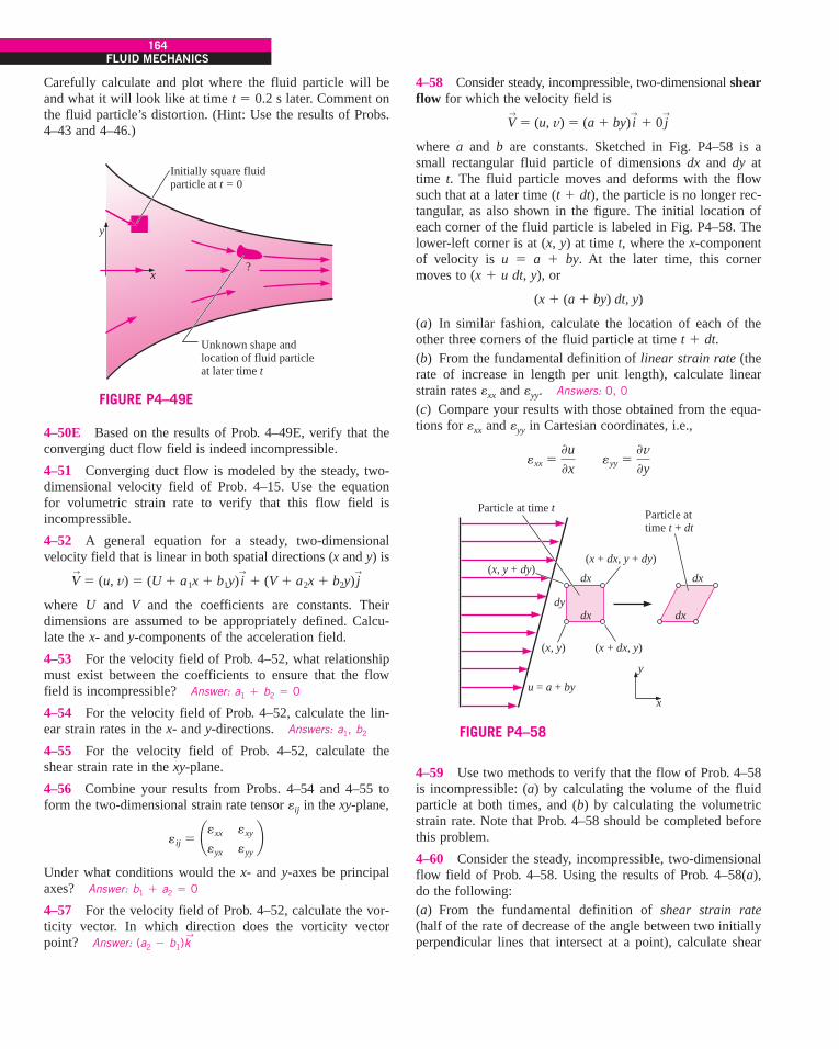
Carefully calculate and plot where the fluid particle will beand what it will look like at time t ! 0.2 s later. Comment onthe fluid particle’s distortion. (Hint: Use the results of Probs.4–43 and 4–46.)

164FLUID MECHANICS

4–58 Consider steady, incompressible, two-dimensional shearflow for which the velocity field is

where a and b are constants. Sketched in Fig. P4–58 is asmall rectangular fluid particle of dimensions dx and dy attime t. The fluid particle moves and deforms with the flowsuch that at a later time (t # dt), the particle is no longer rec-tangular, as also shown in the figure. The initial location ofeach corner of the fluid particle is labeled in Fig. P4–58. Thelower-left corner is at (x, y) at time t, where the x-componentof velocity is u ! a # by. At the later time, this cornermoves to (x # u dt, y), or

(a) In similar fashion, calculate the location of each of theother three corners of the fluid particle at time t # dt.(b) From the fundamental definition of linear strain rate (therate of increase in length per unit length), calculate linearstrain rates exx and eyy. Answers: 0, 0

(c) Compare your results with those obtained from the equa-tions for exx and eyy in Cartesian coordinates, i.e.,

exx !$u$x eyy !

$v$y

(x # (a # by) dt, y)

V!

! (u, v) ! (a # by) i!

# 0 j!

Initially square fluid particle at t = 0

Unknown shape and location of fluid particle at later time t

y

x?

FIGURE P4–49E

4–50E Based on the results of Prob. 4–49E, verify that theconverging duct flow field is indeed incompressible.

4–51 Converging duct flow is modeled by the steady, two-dimensional velocity field of Prob. 4–15. Use the equationfor volumetric strain rate to verify that this flow field isincompressible.

4–52 A general equation for a steady, two-dimensionalvelocity field that is linear in both spatial directions (x and y) is

where U and V and the coefficients are constants. Theirdimensions are assumed to be appropriately defined. Calcu-late the x- and y-components of the acceleration field.

4–53 For the velocity field of Prob. 4–52, what relationshipmust exist between the coefficients to ensure that the flowfield is incompressible? Answer: a1 # b2 ! 0

4–54 For the velocity field of Prob. 4–52, calculate the lin-ear strain rates in the x- and y-directions. Answers: a1, b2

4–55 For the velocity field of Prob. 4–52, calculate theshear strain rate in the xy-plane.

4–56 Combine your results from Probs. 4–54 and 4–55 toform the two-dimensional strain rate tensor eij in the xy-plane,

Under what conditions would the x- and y-axes be principalaxes? Answer: b1 # a2 ! 0

4–57 For the velocity field of Prob. 4–52, calculate the vor-ticity vector. In which direction does the vorticity vectorpoint? Answer: (a2 " b1)k

!

eij ! ¢exx exy

eyx eyy !

V!

! (u, v) ! (U # a1x # b1y) i!

# (V # a2x # b2y) j!

Particle at time t Particle attime t + dt

y

x

(x + dx, y + dy)

u = a + by

dy

(x + dx, y)

(x, y + dy)

(x, y)

dx dx

dx dx

FIGURE P4–58

4–59 Use two methods to verify that the flow of Prob. 4–58is incompressible: (a) by calculating the volume of the fluidparticle at both times, and (b) by calculating the volumetricstrain rate. Note that Prob. 4–58 should be completed beforethis problem.

4–60 Consider the steady, incompressible, two-dimensionalflow field of Prob. 4–58. Using the results of Prob. 4–58(a),do the following:(a) From the fundamental definition of shear strain rate(half of the rate of decrease of the angle between two initiallyperpendicular lines that intersect at a point), calculate shear

cen72367_ch04.qxd 12/1/04 6:20 PM Page 164

CHAPTER 4165

strain rate exy in the xy-plane. (Hint: Use the lower edge andthe left edge of the fluid particle, which intersect at 90* at thelower-left corner of the particle at the initial time.)(b) Compare your results with those obtained from the equa-tion for exy in Cartesian coordinates, i.e.,

Answers: (a) b/2, (b) b/2

4–61 Consider the steady, incompressible, two-dimensionalflow field of Prob. 4–58. Using the results of Prob. 4–58(a),do the following:(a) From the fundamental definition of the rate of rotation(average rotation rate of two initially perpendicular lines thatintersect at a point), calculate the rate of rotation of the fluidparticle in the xy-plane, vz. (Hint: Use the lower edge and theleft edge of the fluid particle, which intersect at 90* at thelower-left corner of the particle at the initial time.)(b) Compare your results with those obtained from the equa-tion for vz in Cartesian coordinates, i.e.,

Answers: (a) "b/2, (b) "b/2

4–62 From the results of Prob. 4–61,(a) Is this flow rotational or irrotational?(b) Calculate the z-component of vorticity for this flow field.

4–63 A two-dimensional fluid element of dimensions dxand dy translates and distorts as shown in Fig. P4–63 duringthe infinitesimal time period dt ! t2 " t1. The velocity com-

vz !12 ¢$v

$x"

$u$y!

exy !12 ¢$u

$y#

$v$x!

ponents at point P at the initial time are u and v in the x- andy-directions, respectively. Show that the magnitude of the rateof rotation (angular velocity) about point P in the xy-plane is

4–64 A two-dimensional fluid element of dimensions dxand dy translates and distorts as shown in Fig. P4–63 duringthe infinitesimal time period dt ! t2 " t1. The velocity com-ponents at point P at the initial time are u and v in the x- andy-directions, respectively. Consider the line segment PA inFig. P4–63, and show that the magnitude of the linear strainrate in the x-direction is

4–65 A two-dimensional fluid element of dimensions dxand dy translates and distorts as shown in Fig. P4–63 duringthe infinitesimal time period dt ! t2 " t1. The velocity com-ponents at point P at the initial time are u and v in the x- andy-directions, respectively. Show that the magnitude of theshear strain rate about point P in the xy-plane is

4–66 Consider a steady, two-dimensional, incompressibleflow field in the xy-plane. The linear strain rate in the x-direction is 2.5 s"1. Calculate the linear strain rate in the y-direction.

4–67 A cylindrical tank of water rotates in solid-body rota-tion, counterclockwise about its vertical axis (Fig. P4–67) atangular speed n

.! 360 rpm. Calculate the vorticity of fluid

particles in the tank. Answer: 75.4 k!

rad/s

exy !12 ¢$u

$y#

$v$x!

exx !$u$x

vz !12 ¢$v

$x"

$u$y!165

CHAPTER 4

y

x

Fluid elementat time t2

Fluid elementat time t1

Line a

Line b

Line b

Line a

P+

B+

B

dy

dxAu

P

v

ab

p/2

aa

A+

FIGURE P4–63

n*

Liquid

Free surface

zrrim

r

FIGURE P4–67

cen72367_ch04.qxd 12/1/04 6:20 PM Page 165

4–68 A cylindrical tank of water rotates about its verticalaxis (Fig. P4–67). A PIV system is used to measure the vor-ticity field of the flow. The measured value of vorticity in thez-direction is "55.4 rad/s and is constant to within 10.5 per-cent everywhere that it is measured. Calculate the angularspeed of rotation of the tank in rpm. Is the tank rotatingclockwise or counterclockwise about the vertical axis?

4–69 A cylindrical tank of radius rrim ! 0.35 m rotates aboutits vertical axis (Fig. P4–67). The tank is partially filled withoil. The speed of the rim is 2.6 m/s in the counterclockwisedirection (looking from the top), and the tank has been spin-ning long enough to be in solid-body rotation. For any fluidparticle in the tank, calculate the magnitude of the componentof vorticity in the vertical z-direction. Answer: 15.0 rad/s

4–70C Explain the relationship between vorticity and rota-tionality.

4–71 Consider a two-dimensional, incompressible flowfield in which an initially square fluid particle moves anddeforms. The fluid particle dimension is a at time t and isaligned with the x- and y-axes as sketched in Fig. P4–71. Atsome later time, the particle is still aligned with the x- and y-axes, but has deformed into a rectangle of horizontal length2a. What is the vertical length of the rectangular fluid particleat this later time?

166FLUID MECHANICS

4–74 Consider fully developed Couette flow—flow betweentwo infinite parallel plates separated by distance h, with thetop plate moving and the bottom plate stationary as illustratedin Fig. P4–74. The flow is steady, incompressible, and two-dimensional in the xy-plane. The velocity field is given by

Is this flow rotational or irrotational? If it is rotational, calcu-late the vorticity component in the z-direction. Do fluid parti-cles in this flow rotate clockwise or counterclockwise?Answers: yes, "V/h, clockwise

V!

! (u, v) ! V y

h i!

# 0 j!

y

x

a

a

FIGURE P4–71

x

yh u =V

yh

V

FIGURE P4–74

4–75 For the Couette flow of Fig. P4–74, calculate the lin-ear strain rates in the x- and y-directions, and calculate theshear strain rate exy.

4–76 Combine your results from Prob. 4–75 to form thetwo-dimensional strain rate tensor eij,

Are the x- and y-axes principal axes?

Reynolds Transport Theorem4–77C True or false: For each statement, choose whetherthe statement is true or false and discuss your answer briefly.(a) The Reynolds transport theorem is useful for transform-ing conservation equations from their naturally occurringcontrol volume forms to their system forms.(b) The Reynolds transport theorem is applicable only tonondeforming control volumes.(c) The Reynolds transport theorem can be applied to bothsteady and unsteady flow fields.(d) The Reynolds transport theorem can be applied to bothscalar and vector quantities.

4–78 Consider the general form of the Reynolds transporttheorem (RTT) given by

dBsys

dt!

ddt

#CV

rb dV # #CS

rbV!

r & n! dA

eij ! ¢exx exy

eyx eyy !

4–72 Consider a two-dimensional, compressible flow fieldin which an initially square fluid particle moves and deforms.The fluid particle dimension is a at time t and is aligned withthe x- and y-axes as sketched in Fig. P4–71. At some latertime, the particle is still aligned with the x- and y-axes buthas deformed into a rectangle of horizontal length 1.06a andvertical length 0.931a. (The particle’s dimension in the z-direction does not change since the flow is two-dimensional.)By what percentage has the density of the fluid particleincreased or decreased?

4–73 Consider the following steady, three-dimensional veloc-ity field:

Calculate the vorticity vector as a function of space (x, y, z).

! (3.0 # 2.0x " y) i!

# (2.0x " 2.0y) j!

# (0.5xy)k!

V!

! (u, v, w)

cen72367_ch04.qxd 12/1/04 6:20 PM Page 166

CHAPTER 4167

where V!

r is the velocity of the fluid relative to the controlsurface. Let Bsys be the mass m of a system of fluid particles.We know that for a system, dm/dt ! 0 since no mass canenter or leave the system by definition. Use the given equa-tion to derive the equation of conservation of mass for a con-trol volume.

4–79 Consider the general form of the Reynolds transporttheorem (RTT) given by Prob. 4–78. Let Bsys be the linearmomentum mV

!of a system of fluid particles. We know that

for a system, Newton’s second law is

Use the equation of Prob. 4–78 and this equation to derivethe equation of conservation of linear momentum for a con-trol volume.

4–80 Consider the general form of the Reynolds transporttheorem (RTT) given in Prob. 4–78. Let Bsys be the angularmomentum H

!! r! . mV

!of a system of fluid particles,

where r! is the moment arm. We know that for a system, con-servation of angular momentum can be expressed as

where 2 M!

is the net moment applied to the system. Use theequation given in Prob. 4–78 and this equation to derive theequation of conservation of angular momentum for a controlvolume.

4–81 Reduce the following expression as far as possible:

(Hint: Use the one-dimensional Leibnitz theorem.) Answer:

Review Problems4–82 Consider fully developed two-dimensional Poiseuilleflow—flow between two infinite parallel plates separated bydistance h, with both the top plate and bottom plate station-ary, and a forced pressure gradient dP/dx driving the flow asillustrated in Fig. P4–82. (dP/dx is constant and negative.)

Be"B2t2

" Ae"A2t2

F(t) !ddt

#x!Bt

x!At

e"2x2

dx

a M!

!ddt

H!

sys

a F!

! ma!

! mdV

!

dt!

ddt

(mV!

)sys

The flow is steady, incompressible, and two-dimensional inthe xy-plane. The velocity components are given by

where m is the fluid’s viscosity. Is this flow rotational or irro-tational? If it is rotational, calculate the vorticity componentin the z-direction. Do fluid particles in this flow rotate clock-wise or counterclockwise?

4–83 For the two-dimensional Poiseuille flow of Prob. 4–82,calculate the linear strain rates in the x- and y-directions, andcalculate the shear strain rate exy.

4–84 Combine your results from Prob. 4–83 to form thetwo-dimensional strain rate tensor eij in the xy-plane,

Are the x- and y-axes principal axes?

4–85 Consider the two-dimensional Poiseuille flow ofProb. 4–82. The fluid between the plates is water

at 40*C. Let the gap height h ! 1.6 mm and the pressure gra-dient dP/dx ! "230 N/m3. Calculate and plot seven path-lines from t ! 0 to t ! 10 s. The fluid particles are releasedat x ! 0 and at y ! 0.2, 0.4, 0.6, 0.8, 1.0, 1.2, and 1.4 mm.

4–86 Consider the two-dimensional Poiseuille flow ofProb. 4–82. The fluid between the plates is

water at 40*C. Let the gap height h ! 1.6 mm and the pres-sure gradient dP/dx ! "230 N/m3. Calculate and plot sevenstreaklines generated from a dye rake that introduces dyestreaks at x ! 0 and at y ! 0.2, 0.4, 0.6, 0.8, 1.0, 1.2, and 1.4 mm (Fig. P4–86). The dye is introduced from t ! 0 to t ! 10 s, and the streaklines are to be plotted at t ! 10 s.

eij ! ¢exx exy

eyx eyy !

u !1

2m dPdx

(y 2 " hy) v ! 0

167CHAPTER 4

x

y

u(y)

h

FIGURE P4–82

4–87 Repeat Prob. 4–86 except that the dye is intro-duced from t ! 0 to t ! 10 s, and the streaklines

are to be plotted at t ! 12 s instead of 10 s.

4–88 Compare the results of Probs. 4–86 and 4–87and comment about the linear strain rate in the

x-direction.

4–89 Consider the two-dimensional Poiseuille flow ofProb. 4–82. The fluid between the plates is water

x

y

u(y)Dye rake

h

FIGURE P4–86

cen72367_ch04.qxd 12/1/04 6:20 PM Page 167

at 40*C. Let the gap height h ! 1.6 mm and the pressure gra-dient dP/dx ! "230 N/m3. Imagine a hydrogen bubble wirestretched vertically through the channel at x ! 0 (Fig. P4–89).The wire is pulsed on and off such that bubbles are producedperiodically to create timelines. Five distinct timelines aregenerated at t ! 0, 2.5, 5.0, 7.5, and 10.0 s. Calculate and plotwhat these five timelines look like at time t ! 12.5 s.

168FLUID MECHANICS

4–92 Combine your results from Prob. 4–91 to form theaxisymmetric strain rate tensor eij,

Are the x- and r-axes principal axes?

4–93 We approximate the flow of air into a vacuum cleanerattachment by the following velocity components in the cen-terplane (the xy-plane):

and

where b is the distance of the attachment above the floor, L isthe length of the attachment, and V

.is the volume flow rate of

air being sucked up into the hose (Fig. P4–93). Determine thelocation of any stagnation point(s) in this flow field. Answer:at the origin

v !"V#

y

pL

x 2 # y 2 " b2

x 4 # 2x 2y 2 # 2x 2b2 # y 4 " 2y 2b2 # b4

u !"V#x

pL

x 2 # y 2 # b2

x 4 # 2x 2y 2 # 2x 2b2 # y 4 " 2y 2b2 # b4

eij ! aerr

exr

erx

exxb

x

u(y)H2 wire

hy

FIGURE P4–89

u(r)

D

R

u

r

x

FIGURE P4–90

4–90 Consider fully developed axisymmetric Poiseuilleflow—flow in a round pipe of radius R (diameter D ! 2R),with a forced pressure gradient dP/dx driving the flow asillustrated in Fig. P4–90. (dP/dx is constant and negative.)The flow is steady, incompressible, and axisymmetric aboutthe x-axis. The velocity components are given by

where m is the fluid’s viscosity. Is this flow rotational or irro-tational? If it is rotational, calculate the vorticity componentin the circumferential (u) direction and discuss the sign of therotation.

u !1

4m dPdx

(r 2 " R2) ur ! 0 uu ! 0

4–91 For the axisymmetric Poiseuille flow of Prob. 4–90,calculate the linear strain rates in the x- and r-directions, andcalculate the shear strain rate exr. The strain rate tensor incylindrical coordinates (r, u, x) and (ur, uu, ux), is

! ¶ $ur

$r12 ar

$

$r auu

rb #

1r $ur

$ub

12 a$ur

$x#

$ux

$rb

12 ar

$

$r auu

rb #

1r $ur

$ub

1r $uu$u

#ur

r12 a1

r $ux

$u#

$uu$xb

12 a$ur

$x#

$ux

$rb

12 a1

r $ux

$u#

$uu$xb

$ux

$x

# eij ! £err

eurexr

eru

euuexu

erx

euxexx

"Floor

V

y

L

z xb

·

FIGURE P4–93

4–94 Consider the vacuum cleaner of Prob. 4–93. For thecase where b ! 2.0 cm, L ! 35 cm, and V

.! 0.1098 m3/s,

create a velocity vector plot in the upper half of the xy-planefrom x ! "3 cm to 3 cm and from y ! 0 cm to 2.5 cm. Drawas many vectors as you need to get a good feel of the flowfield. Note: The velocity is infinite at the point (x, y) ! (0,2.0 cm), so do not attempt to draw a velocity vector at thatpoint.

4–95 Consider the approximate velocity field given for thevacuum cleaner of Prob. 4–93. Calculate the flow speedalong the floor. Dust particles on the floor are most likely tobe sucked up by the vacuum cleaner at the location of maxi-

cen72367_ch04.qxd 12/1/04 6:20 PM Page 168

CHAPTER 4169

mum speed. Where is that location? Do you think the vacuumcleaner will do a good job at sucking up dust directly belowthe inlet (at the origin)? Why or why not?

4–96 Consider a steady, two-dimensional flow field in thexy-plane whose x-component of velocity is given by

where a, b, and c are constants with appropriate dimensions.Of what form does the y-component of velocity need to be inorder for the flow field to be incompressible? In other words,generate an expression for v as a function of x, y, and theconstants of the given equation such that the flow is incom-pressible. Answer: "2b(x " c)y # f(x)

4–97 There are numerous occasions in which a fairly uni-form free-stream flow encounters a long circular cylinderaligned normal to the flow (Fig. P4–97). Examples include airflowing around a car antenna, wind blowing against a flagpole or telephone pole, wind hitting electrical wires, andocean currents impinging on the submerged round beams thatsupport oil platforms. In all these cases, the flow at the rear ofthe cylinder is separated and unsteady, and usually turbulent.However, the flow in the front half of the cylinder is muchmore steady and predictable. In fact, except for a very thinboundary layer near the cylinder surface, the flow field maybe approximated by the following steady, two-dimensionalvelocity components in the xy- or ru-plane:

ur ! V cos ua1 "a2

r 2b uu ! "V sin ua1 #a2

r 2b

u ! a # b(x " c)2

4–99 Consider the upstream half (x ) 0) of the flowfield of Prob. 4–97 (flow over a circular cylin-

der). We introduce a parameter called the stream function c,which is constant along streamlines in two-dimensionalflows such as the one being considered here (Fig. P4–99).The velocity field of Prob. 4–97 corresponds to a streamfunction given by

(a) Setting c to a constant, generate an equation for astreamline. (Hint: Use the quadratic rule to solve for r as afunction of u.)(b) For the particular case in which V ! 1.00 m/s and cylinderradius a ! 10.0 cm, plot several streamlines in the upstreamhalf of the flow (90* ) u ) 270*). For consistency, plot inthe range "0.4 m ) x ) 0 m, "0.2 m ) y ) 0.2 m, withstream function values evenly spaced between "0.16 m2/sand 0.16 m2/s.

c ! V sin uar "a2

rb

169CHAPTER 4

Vy

r = a

r

u

x

FIGURE P4–97

4–100 Consider the flow field of Prob. 4–97 (flow over acircular cylinder). Calculate the two linear strain rates in theru-plane; i.e., calculate err and euu. Discuss whether fluid linesegments stretch (or shrink) in this flow field. (Hint: Thestrain rate tensor in cylindrical coordinates is given in Prob.4–91.)

4–101 Based on your results of Prob. 4–100, discuss thecompressibility (or incompressibility) of this flow. Answer:flow is incompressible

4–102 Consider the flow field of Prob. 4–97 (flow over acircular cylinder). Calculate eru, the shear strain rate in theru-plane. Discuss whether fluid particles in this flow deformwith shear or not. (Hint: The strain rate tensor in cylindricalcoordinates is given in Prob. 4–91.)

Streamlines

y

x

c4

c3

c2

c1

FIGURE P4–99

Is this flow field rotational or irrotational? Explain.

4–98 Consider the flow field of Prob. 4–97 (flow over a cir-cular cylinder). Consider only the front half of the flow (x) 0). There is one stagnation point in the front half of theflow field. Where is it? Give your answer in both cylindrical(r, u) coordinates and Cartesian (x, y) coordinates.

cen72367_ch04.qxd 12/1/04 6:20 PM Page 169

cen72367_ch04.qxd 12/1/04 6:20 PM Page 170

M A S S , B E R N O U L L I , A N D E N E R G Y E Q U AT I O N S

This chapter deals with three equations commonly used in fluidmechanics: the mass, Bernoulli, and energy equations. The mass equa-tion is an expression of the conservation of mass principle. The

Bernoulli equation is concerned with the conservation of kinetic, potential,and flow energies of a fluid stream and their conversion to each other inregions of flow where net viscous forces are negligible and where otherrestrictive conditions apply. The energy equation is a statement of the con-servation of energy principle. In fluid mechanics, it is found convenient toseparate mechanical energy from thermal energy and to consider the con-version of mechanical energy to thermal energy as a result of frictionaleffects as mechanical energy loss. Then the energy equation becomes themechanical energy balance.

We start this chapter with an overview of conservation principles and theconservation of mass relation. This is followed by a discussion of variousforms of mechanical energy and the efficiency of mechanical work devicessuch as pumps and turbines. Then we derive the Bernoulli equation byapplying Newton’s second law to a fluid element along a streamline anddemonstrate its use in a variety of applications. We continue with the devel-opment of the energy equation in a form suitable for use in fluid mechanicsand introduce the concept of head loss. Finally, we apply the energy equa-tion to various engineering systems.

171

CHAPTER

5OBJECTIVESWhen you finish reading this chapter, youshould be able to

! Apply the mass equation tobalance the incoming andoutgoing flow rates in a flowsystem

! Recognize various forms ofmechanical energy, and workwith energy conversionefficiencies

! Understand the use andlimitations of the Bernoulliequation, and apply it to solve avariety of fluid flow problems

! Work with the energy equationexpressed in terms of heads, anduse it to determine turbinepower output and pumpingpower requirements

cen72367_ch05.qxd 10/29/04 2:24 PM Page 171

5–1 ! INTRODUCTIONYou are already familiar with numerous conservation laws such as the lawsof conservation of mass, conservation of energy, and conservation ofmomentum. Historically, the conservation laws are first applied to a fixedquantity of matter called a closed system or just a system, and then extendedto regions in space called control volumes. The conservation relations arealso called balance equations since any conserved quantity must balanceduring a process. We now give a brief description of the conservation ofmass, momentum, and energy relations (Fig. 5–1).

Conservation of MassThe conservation of mass relation for a closed system undergoing a changeis expressed as msys ! constant or dmsys/dt ! 0, which is a statement of theobvious that the mass of the system remains constant during a process. Fora control volume (CV), mass balance is expressed in the rate form as

Conservation of mass: (5–1)

where m. in and m. out are the total rates of mass flow into and out of the con-trol volume, respectively, and dmCV/dt is the rate of change of mass withinthe control volume boundaries. In fluid mechanics, the conservation of massrelation written for a differential control volume is usually called the conti-nuity equation. Conservation of mass is discussed in Section 5–2.

Conservation of MomentumThe product of the mass and the velocity of a body is called the linearmomentum or just the momentum of the body, and the momentum of a rigidbody of mass m moving with a velocity V

!is mV

!. Newton’s second law states

that the acceleration of a body is proportional to the net force acting on itand is inversely proportional to its mass, and that the rate of change of themomentum of a body is equal to the net force acting on the body. Therefore,the momentum of a system remains constant when the net force acting on itis zero, and thus the momentum of such systems is conserved. This is knownas the conservation of momentum principle. In fluid mechanics, Newton’ssecond law is usually referred to as the linear momentum equation, which isdiscussed in Chap. 6 together with the angular momentum equation.

Conservation of EnergyEnergy can be transferred to or from a closed system by heat or work, andthe conservation of energy principle requires that the net energy transfer toor from a system during a process be equal to the change in the energy con-tent of the system. Control volumes involve energy transfer via mass flowalso, and the conservation of energy principle, also called the energy bal-ance, is expressed as

Conservation of energy: (5–2)

where E.

in and E.

out are the total rates of energy transfer into and out of thecontrol volume, respectively, and dECV/dt is the rate of change of energywithin the control volume boundaries. In fluid mechanics, we usually limit

E#in " E

#out !

dECV

dt

m#

in " m#

out !dmCV

dt

172FLUID MECHANICS

FIGURE 5–1Many fluid flow devices such as thisPelton wheel hydraulic turbine areanalyzed by applying the conservationof mass, momentum, and energyprinciples.Courtesy of Hydro Tasmania, www.hydro.com.au.Used by permission.

cen72367_ch05.qxd 10/29/04 2:24 PM Page 172

173CHAPTER 5

our consideration to mechanical forms of energy only. Conservation ofenergy is discussed in Section 5–6.

5–2 ! CONSERVATION OF MASSThe conservation of mass principle is one of the most fundamental princi-ples in nature. We are all familiar with this principle, and it is not difficult tounderstand. As the saying goes, You cannot have your cake and eat it too! Aperson does not have to be a scientist to figure out how much vinegar-and-oil dressing will be obtained by mixing 100 g of oil with 25 g of vinegar.Even chemical equations are balanced on the basis of the conservation ofmass principle. When 16 kg of oxygen reacts with 2 kg of hydrogen, 18 kgof water is formed (Fig. 5–2). In an electrolysis process, the water will sep-arate back to 2 kg of hydrogen and 16 kg of oxygen.

Mass, like energy, is a conserved property, and it cannot be created ordestroyed during a process. However, mass m and energy E can be con-verted to each other according to the well-known formula proposed byAlbert Einstein (1879–1955):

(5–3)

where c is the speed of light in a vacuum, which is c ! 2.9979 # 108 m/s.This equation suggests that the mass of a system changes when its energychanges. However, for all energy interactions encountered in practice, withthe exception of nuclear reactions, the change in mass is extremely small andcannot be detected by even the most sensitive devices. For example, when1 kg of water is formed from oxygen and hydrogen, the amount of energyreleased is 15,879 kJ, which corresponds to a mass of 1.76 # 10"10 kg. Amass of this magnitude is beyond the accuracy required by practically allengineering calculations and thus can be disregarded.

For closed systems, the conservation of mass principle is implicitly used byrequiring that the mass of the system remain constant during a process. Forcontrol volumes, however, mass can cross the boundaries, and so we mustkeep track of the amount of mass entering and leaving the control volume.

Mass and Volume Flow RatesThe amount of mass flowing through a cross section per unit time is calledthe mass flow rate and is denoted by m. . The dot over a symbol is used toindicate time rate of change.

A fluid flows into or out of a control volume, usually through pipes orducts. The differential mass flow rate of fluid flowing across a small areaelement dAc in a cross section of the pipe is proportional to dAc itself, thefluid density r, and the component of the flow velocity normal to dAc,which we denote as Vn, and is expressed as (Fig. 5–3)

(5–4)

Note that both d and d are used to indicate differential quantities, but d istypically used for quantities (such as heat, work, and mass transfer) that arepath functions and have inexact differentials, while d is used for quantities(such as properties) that are point functions and have exact differentials. Forflow through an annulus of inner radius r1 and outer radius r2, for example,

dm#

! rVn dAc

E ! mc2

2 kgH2

16 kgO2

18 kgH2O

FIGURE 5–2Mass is conserved even during

chemical reactions.

!

!

dAcVn

V

n

Control surface

FIGURE 5–3The normal velocity Vn for a surface

is the component of velocityperpendicular to the surface.

cen72367_ch05.qxd 10/29/04 2:25 PM Page 173

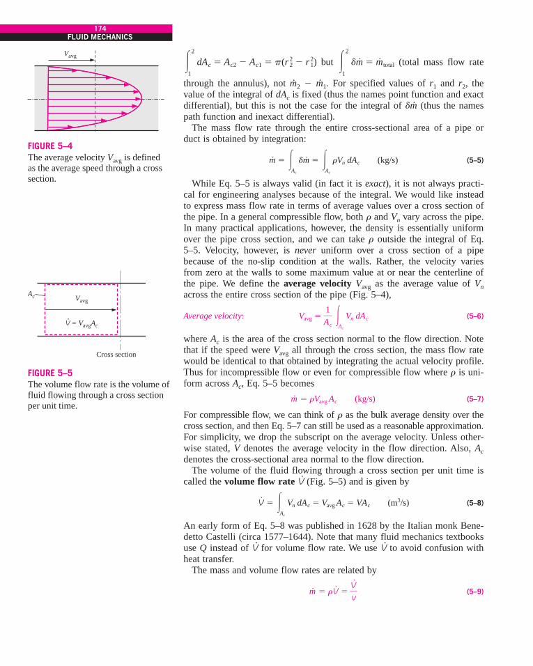
174FLUID MECHANICS

but (total mass flow rate

through the annulus), not m. 2 " m. 1. For specified values of r1 and r2, thevalue of the integral of dAc is fixed (thus the names point function and exactdifferential), but this is not the case for the integral of dm. (thus the namespath function and inexact differential).

The mass flow rate through the entire cross-sectional area of a pipe orduct is obtained by integration:

(5–5)

While Eq. 5–5 is always valid (in fact it is exact), it is not always practi-cal for engineering analyses because of the integral. We would like insteadto express mass flow rate in terms of average values over a cross section ofthe pipe. In a general compressible flow, both r and Vn vary across the pipe.In many practical applications, however, the density is essentially uniformover the pipe cross section, and we can take r outside the integral of Eq.5–5. Velocity, however, is never uniform over a cross section of a pipebecause of the no-slip condition at the walls. Rather, the velocity variesfrom zero at the walls to some maximum value at or near the centerline ofthe pipe. We define the average velocity Vavg as the average value of Vnacross the entire cross section of the pipe (Fig. 5–4),

Average velocity: (5–6)

where Ac is the area of the cross section normal to the flow direction. Notethat if the speed were Vavg all through the cross section, the mass flow ratewould be identical to that obtained by integrating the actual velocity profile.Thus for incompressible flow or even for compressible flow where r is uni-form across Ac, Eq. 5–5 becomes

(5–7)

For compressible flow, we can think of r as the bulk average density over thecross section, and then Eq. 5–7 can still be used as a reasonable approximation.For simplicity, we drop the subscript on the average velocity. Unless other-wise stated, V denotes the average velocity in the flow direction. Also, Acdenotes the cross-sectional area normal to the flow direction.

The volume of the fluid flowing through a cross section per unit time iscalled the volume flow rate V

.(Fig. 5–5) and is given by

(5–8)

An early form of Eq. 5–8 was published in 1628 by the Italian monk Bene-detto Castelli (circa 1577–1644). Note that many fluid mechanics textbooksuse Q instead of V

.for volume flow rate. We use V

.to avoid confusion with

heat transfer.The mass and volume flow rates are related by

(5–9)m#

! rV#

!V#

v

V#

! !Ac

Vn dAc ! Vavg Ac ! VAc (m3/s)

m#

! rVavg Ac (kg/s)

Vavg !1Ac

!Ac

Vn dAc

m#

! !Ac

dm#

! !Ac

rVn dAc (kg/s)

!2

1

dm#

! m#

total!2

1

dAc ! Ac2 " Ac1 ! p(r 22 " r 1

2)Vavg

FIGURE 5–4The average velocity Vavg is defined as the average speed through a crosssection.

Vavg

Cross section

Ac

V = VavgAc

FIGURE 5–5The volume flow rate is the volume offluid flowing through a cross sectionper unit time.

cen72367_ch05.qxd 10/29/04 2:25 PM Page 174

175CHAPTER 5

where v is the specific volume. This relation is analogous to m ! rV !V/v, which is the relation between the mass and the volume of a fluid in acontainer.

Conservation of Mass PrincipleThe conservation of mass principle for a control volume can be expressedas: The net mass transfer to or from a control volume during a time interval$t is equal to the net change (increase or decrease) in the total mass withinthe control volume during $t. That is,

or

(5–10)

where $mCV ! mfinal – minitial is the change in the mass of the control vol-ume during the process (Fig. 5–6). It can also be expressed in rate form as

(5–11)

where m. in and m. out are the total rates of mass flow into and out of the con-trol volume, and dmCV/dt is the rate of change of mass within the controlvolume boundaries. Equations 5–10 and 5–11 are often referred to as themass balance and are applicable to any control volume undergoing anykind of process.

Consider a control volume of arbitrary shape, as shown in Fig. 5–7. Themass of a differential volume dV within the control volume is dm ! r dV.The total mass within the control volume at any instant in time t is deter-mined by integration to be

Total mass within the CV: (5–12)

Then the time rate of change of the amount of mass within the control vol-ume can be expressed as

Rate of change of mass within the CV: (5–13)

For the special case of no mass crossing the control surface (i.e., the controlvolume resembles a closed system), the conservation of mass principlereduces to that of a system that can be expressed as dmCV/dt ! 0. This rela-tion is valid whether the control volume is fixed, moving, or deforming.

Now consider mass flow into or out of the control volume through a differ-ential area dA on the control surface of a fixed control volume. Let n! be theoutward unit vector of dA normal to dA and V

!be the flow velocity at dA rel-

ative to a fixed coordinate system, as shown in Fig. 5–7. In general, thevelocity may cross dA at an angle u off the normal of dA, and the mass flowrate is proportional to the normal component of velocity V

!

n ! V!

cos u rang-ing from a maximum outflow of V

!for u ! 0 (flow is normal to dA) to a min-

imum of zero for u ! 90° (flow is tangent to dA) to a maximum inflow of V!

for u ! 180° (flow is normal to dA but in the opposite direction). Making

dmCV

dt!

ddt

!CV

r dV

mCV ! !CV

r dV

m#

in " m#

out ! dmCV/dt (kg/s)

min " mout ! $mCV (kg)

aTotal mass enteringthe CV during $t

b " aTotal mass leavingthe CV during $t

b ! a Net change in masswithin the CV during $t

bWater

"mbathtub = min –

mout = 20 kgmin = 50 kg

mout = 30 kg

FIGURE 5–6Conservation of mass principle

for an ordinary bathtub.

!

!

Controlvolume (CV)

Control surface (CS)

dV

dmdA

n

V

u

FIGURE 5–7The differential control volume dVand the differential control surface

dA used in the derivation of theconservation of mass relation.

cen72367_ch05.qxd 10/29/04 2:25 PM Page 175

176FLUID MECHANICS

use of the concept of dot product of two vectors, the magnitude of the nor-mal component of velocity can be expressed as

Normal component of velocity: (5–14)

The mass flow rate through dA is proportional to the fluid density r, normalvelocity Vn, and the flow area dA, and can be expressed as

Differential mass flow rate: (5–15)

The net flow rate into or out of the control volume through the entire con-trol surface is obtained by integrating dm. over the entire control surface,

Net mass flow rate: (5–16)

Note that V!

· n! ! V cos u is positive for u % 90° (outflow) and negative foru & 90° (inflow). Therefore, the direction of flow is automaticallyaccounted for, and the surface integral in Eq. 5–16 directly gives the netmass flow rate. A positive value for m. net indicates net outflow, and a nega-tive value indicates a net inflow of mass.

Rearranging Eq. 5–11 as dmCV/dt ' m. out " m. in ! 0, the conservation ofmass relation for a fixed control volume can then be expressed as

General conservation of mass: (5–17)

It states that the time rate of change of mass within the control volume plusthe net mass flow rate through the control surface is equal to zero.

The general conservation of mass relation for a control volume can alsobe derived using the Reynolds transport theorem (RTT) by taking the prop-erty B to be the mass m (Chap. 4). Then we have b ! 1 since dividing themass by mass to get the property per unit mass gives unity. Also, the massof a system is constant, and thus its time derivative is zero. That is, dmsys /dt! 0. Then the Reynolds transport equation reduces immediately to Eq.5–17, as shown in Fig. 5–8, and thus illustrates that the Reynolds transporttheorem is a very powerful tool indeed. In Chap. 6 we apply the RTT toobtain the linear and angular momentum equations for control volumes.

Splitting the surface integral in Eq. 5–17 into two parts—one for the out-going flow streams (positive) and one for the incoming streams (negative)—the general conservation of mass relation can also be expressed as

(5–18)

where A represents the area for an inlet or outlet, and the summation signsare used to emphasize that all the inlets and outlets are to be considered.Using the definition of mass flow rate, Eq. 5–18 can also be expressed as

(5–19)

There is considerable flexibility in the selection of a control volume whensolving a problem. Several control volume choices may be correct, but someare more convenient to work with. A control volume should not introduceany unnecessary complications. The proper choice of a control volume canmake the solution of a seemingly complicated problem rather easy. A simple

ddt

!CV

r dV ! ain

m#

" aout

m# or dmCV

dt! a

inm#

" aout

m#

ddt

!CV

r dV ' aout

!A

rVn dA " ain

!A

rVn dA ! 0

ddt

!CV

r dV ' !CS

r(V!

( n!) dA ! 0

m#

net ! !CS

dm#

! !CS

rVn dA ! !CS

r(V!

( n!

) dA

dm#

! rVn dA ! r(V cos u) dA ! r(V!

( n!) dA

Vn ! V cos u! V!

( n!

!!

!!= +

B = m b = 1 b = 1

dBsys

dtV

d

dtCV! rb( · n ) dA

CS!

= +dmsys

dtV

d

dtCV! r( · n ) dA

CS!r dV

rb dV

FIGURE 5–8The conservation of mass equation is obtained by replacing B in theReynolds transport theorem by mass m, and b by 1 (m per unit mass ! m/m ! 1).

cen72367_ch05.qxd 10/29/04 2:25 PM Page 176

177CHAPTER 5

V!n

A V

m = rVA

FIGURE 5–9A control surface should always be

selected normal to flow at all locationswhere it crosses the fluid flow to avoid

complications, even though the resultis the same.

rule in selecting a control volume is to make the control surface normal toflow at all locations where it crosses fluid flow, whenever possible. Thisway the dot product V

!· n! simply becomes the magnitude of the velocity,

and the integral becomes simply rVA (Fig. 5–9).

Moving or Deforming Control VolumesEquations 5–17 and 5–18 are also valid for moving or deforming controlvolumes provided that the absolute velocity V

!is replaced by the relative

velocity V!

r , which is the fluid velocity relative to the control surface (Chap.4). In the case of a nondeforming control volume, relative velocity is thefluid velocity observed by a person moving with the control volume and isexpressed as V

!

r ! V!

" V!

CV, where V!

is the fluid velocity and V!

CV is thevelocity of the control volume, both relative to a fixed point outside. Againnote that this is a vector subtraction.

Some practical problems (such as the injection of medication through theneedle of a syringe by the forced motion of the plunger) involve deformingcontrol volumes. The conservation of mass relations developed can still beused for such deforming control volumes provided that the velocity of thefluid crossing a deforming part of the control surface is expressed relative tothe control surface (that is, the fluid velocity should be expressed relative toa reference frame attached to the deforming part of the control surface). Therelative velocity in this case at any point on the control surface is expressedas V

!

r! V!

" V!

CS, where V!

CS is the local velocity of the control surface at thatpoint relative to a fixed point outside the control volume.

Mass Balance for Steady-Flow ProcessesDuring a steady-flow process, the total amount of mass contained within acontrol volume does not change with time (mCV ! constant). Then the con-servation of mass principle requires that the total amount of mass entering acontrol volume equal the total amount of mass leaving it. For a garden hosenozzle in steady operation, for example, the amount of water entering thenozzle per unit time is equal to the amount of water leaving it per unit time.

When dealing with steady-flow processes, we are not interested in theamount of mass that flows in or out of a device over time; instead, we areinterested in the amount of mass flowing per unit time, that is, the mass flowrate m. . The conservation of mass principle for a general steady-flow systemwith multiple inlets and outlets can be expressed in rate form as (Fig. 5–10)

Steady flow: (5–20)

It states that the total rate of mass entering a control volume is equal to thetotal rate of mass leaving it.

Many engineering devices such as nozzles, diffusers, turbines, compres-sors, and pumps involve a single stream (only one inlet and one outlet). Forthese cases, we denote the inlet state by the subscript 1 and the outlet stateby the subscript 2, and drop the summation signs. Then Eq. 5–20 reduces,for single-stream steady-flow systems, to

Steady flow (single stream): (5–21)m#

1 ! m#

2 ! r1V1 A1 ! r2V2 A2

ain

m#

! aout

m# (kg/s)

!A

r(V!

( n!

) dA

m

CV

˙ 1 = 2 kg/s m2 = 3 kg/s

m3 = m1 + m2 = 5 kg/s˙ ˙ ˙

FIGURE 5–10Conservation of mass principle

for a two-inlet–one-outlet steady-flow system.

Vu!n

Vn = V cos u

A/cos uA V

m = r(V cos u)(A/cos u) = rVA

(a) Control surface at an angle to flow

(b) Control surface normal to flow

cen72367_ch05.qxd 10/29/04 2:25 PM Page 177

Special Case: Incompressible FlowThe conservation of mass relations can be simplified even further when thefluid is incompressible, which is usually the case for liquids. Canceling thedensity from both sides of the general steady-flow relation gives

Steady, incompressible flow: (5–22)

For single-stream steady-flow systems it becomes

Steady, incompressible flow (single stream): (5–23)

It should always be kept in mind that there is no such thing as a “conserva-tion of volume” principle. Therefore, the volume flow rates into and out of asteady-flow device may be different. The volume flow rate at the outlet ofan air compressor is much less than that at the inlet even though the massflow rate of air through the compressor is constant (Fig. 5–11). This is dueto the higher density of air at the compressor exit. For steady flow of liq-uids, however, the volume flow rates, as well as the mass flow rates, remainconstant since liquids are essentially incompressible (constant-density) sub-stances. Water flow through the nozzle of a garden hose is an example ofthe latter case.

The conservation of mass principle is based on experimental observationsand requires every bit of mass to be accounted for during a process. If youcan balance your checkbook (by keeping track of deposits and withdrawals,or by simply observing the “conservation of money” principle), you shouldhave no difficulty applying the conservation of mass principle to engineer-ing systems.

EXAMPLE 5–1 Water Flow through a Garden Hose Nozzle

A garden hose attached with a nozzle is used to fill a 10-gal bucket. Theinner diameter of the hose is 2 cm, and it reduces to 0.8 cm at the nozzleexit (Fig. 5–12). If it takes 50 s to fill the bucket with water, determine(a) the volume and mass flow rates of water through the hose, and (b) theaverage velocity of water at the nozzle exit.

SOLUTION A garden hose is used to fill a water bucket. The volume andmass flow rates of water and the exit velocity are to be determined.Assumptions 1 Water is an incompressible substance. 2 Flow through thehose is steady. 3 There is no waste of water by splashing.Properties We take the density of water to be 1000 kg/m3 ! 1 kg/L.Analysis (a) Noting that 10 gal of water are discharged in 50 s, the volumeand mass flow rates of water are

(b) The cross-sectional area of the nozzle exit is

Ae ! pr 2e ! p(0.4 cm)2 ! 0.5027 cm2 ! 0.5027 # 10"4 m2

m#

! rV#

! (1 kg/L)(0.757 L/s) ! 0.757 kg/s

V#

!V$t

!10 gal

50 s a3.7854 L

1 galb ! 0.757 L/s

V#

1 ! V#

2 ! V1A1 ! V2 A2

ain

V#

! aout

V# (m3/s)

178FLUID MECHANICS

m 1 = 2 kg/s

Aircompressor

m2 = 2 kg/s

V2 = 0.8 m3/s

V1 = 1.4 m3/s

FIGURE 5–11During a steady-flow process,volume flow rates are not necessarilyconserved although mass flow rates are.

Nozzle

BucketGardenhose

FIGURE 5–12Schematic for Example 5–1.

cen72367_ch05.qxd 10/29/04 2:25 PM Page 178

The volume flow rate through the hose and the nozzle is constant. Then theaverage velocity of water at the nozzle exit becomes

Discussion It can be shown that the average velocity in the hose is 2.4 m/s.Therefore, the nozzle increases the water velocity by over six times.

EXAMPLE 5–2 Discharge of Water from a Tank

A 4-ft-high, 3-ft-diameter cylindrical water tank whose top is open to theatmosphere is initially filled with water. Now the discharge plug near the bot-tom of the tank is pulled out, and a water jet whose diameter is 0.5 instreams out (Fig. 5–13). The average velocity of the jet is given by V ! , where h is the height of water in the tank measured from thecenter of the hole (a variable) and g is the gravitational acceleration. Deter-mine how long it will take for the water level in the tank to drop to 2 ft fromthe bottom.

SOLUTION The plug near the bottom of a water tank is pulled out. Thetime it will take for half of the water in the tank to empty is to be deter-mined.Assumptions 1 Water is an incompressible substance. 2 The distancebetween the bottom of the tank and the center of the hole is negligible com-pared to the total water height. 3 The gravitational acceleration is 32.2 ft/s2.Analysis We take the volume occupied by water as the control volume. Thesize of the control volume decreases in this case as the water level drops,and thus this is a variable control volume. (We could also treat this as afixed control volume that consists of the interior volume of the tank by disre-garding the air that replaces the space vacated by the water.) This is obvi-ously an unsteady-flow problem since the properties (such as the amount ofmass) within the control volume change with time.

The conservation of mass relation for a control volume undergoing anyprocess is given in the rate form as

(1)

During this process no mass enters the control volume (m.

in ! 0), and themass flow rate of discharged water can be expressed as

(2)

where Ajet ! pD2jet/4 is the cross-sectional area of the jet, which is constant.

Noting that the density of water is constant, the mass of water in the tank atany time is

(3)

where Atank ! pD2tank/4 is the base area of the cylindrical tank. Substituting

Eqs. 2 and 3 into the mass balance relation (Eq. 1) gives

"r22ghAjet !d(rAtankh)

dt! "r22gh(pD2

jet /4) !r(pD2

tank/4) dh

dt

mCV ! rV ! rAtankh

m#

out ! (rVA)out ! r22ghAjet

m#

in " m#

out !dmCV

dt

12gh

Ve !V#

Ae!

0.757 L/s0.5027 # 10"4 m2 a 1 m3

1000 Lb ! 15.1 m/s

179CHAPTER 5

Water

Air

0 Dtank

Djeth2

h0

h

FIGURE 5–13Schematic for Example 5–2.

cen72367_ch05.qxd 10/29/04 2:25 PM Page 179

Canceling the densities and other common terms and separating the vari-ables give

Integrating from t ! 0 at which h ! h0 to t ! t at which h ! h2 gives

Substituting, the time of discharge is determined to be

Therefore, half of the tank will be emptied in 12.6 min after the dischargehole is unplugged.Discussion Using the same relation with h2 ! 0 gives t ! 43.1 min for thedischarge of the entire amount of water in the tank. Therefore, emptying thebottom half of the tank takes much longer than emptying the top half. Thisis due to the decrease in the average discharge velocity of water withdecreasing h.

5–3 ! MECHANICAL ENERGY AND EFFICIENCYMany fluid systems are designed to transport a fluid from one location toanother at a specified flow rate, velocity, and elevation difference, and thesystem may generate mechanical work in a turbine or it may consumemechanical work in a pump or fan during this process. These systems donot involve the conversion of nuclear, chemical, or thermal energy tomechanical energy. Also, they do not involve any heat transfer in any signif-icant amount, and they operate essentially at constant temperature. Suchsystems can be analyzed conveniently by considering the mechanical formsof energy only and the frictional effects that cause the mechanical energy tobe lost (i.e., to be converted to thermal energy that usually cannot be usedfor any useful purpose).

The mechanical energy can be defined as the form of energy that can beconverted to mechanical work completely and directly by an ideal mechani-cal device such as an ideal turbine. Kinetic and potential energies are thefamiliar forms of mechanical energy. Thermal energy is not mechanicalenergy, however, since it cannot be converted to work directly and com-pletely (the second law of thermodynamics).

A pump transfers mechanical energy to a fluid by raising its pressure, anda turbine extracts mechanical energy from a fluid by dropping its pressure.Therefore, the pressure of a flowing fluid is also associated with its mechan-ical energy. In fact, the pressure unit Pa is equivalent to Pa ! N/m2 !N · m/m3 ! J/m3, which is energy per unit volume, and the product Pv orits equivalent P/r has the unit J/kg, which is energy per unit mass. Note thatpressure itself is not a form of energy. But a pressure force acting on a fluidthrough a distance produces work, called flow work, in the amount of P/rper unit mass. Flow work is expressed in terms of fluid properties, and it isconvenient to view it as part of the energy of a flowing fluid and call it flow

t !24 ft " 22 ft232.2/2 ft/s2

a3 # 12 in0.5 in

b 2

! 757 s ! 12.6 min

!t

0

dt ! "D2

tank

D2jet22g

!h2

h0

dh2h

! t !2h0 " 2h22g/2

aDtank

Djetb 2

dt ! "D2

tank

D2jet

dh22gh

180FLUID MECHANICS

cen72367_ch05.qxd 10/29/04 2:25 PM Page 180

energy. Therefore, the mechanical energy of a flowing fluid can beexpressed on a unit-mass basis as (Fig. 5–14).

where P/r is the flow energy, V2/2 is the kinetic energy, and gz is the poten-tial energy of the fluid, all per unit mass. Then the mechanical energychange of a fluid during incompressible flow becomes

(5–24)

Therefore, the mechanical energy of a fluid does not change during flow ifits pressure, density, velocity, and elevation remain constant. In the absenceof any losses, the mechanical energy change represents the mechanicalwork supplied to the fluid (if $emech & 0) or extracted from the fluid (if$emech % 0).

Consider a container of height h filled with water, as shown in Fig. 5–15,with the reference level selected at the bottom surface. The gage pressureand the potential energy per unit mass are, respectively, PA ! 0 and peA! gh at point A at the free surface, and PB ! rgh and peB ! 0 at point B atthe bottom of the container. An ideal hydraulic turbine would produce thesame work per unit mass wturbine ! gh whether it receives water (or anyother fluid with constant density) from the top or from the bottom of thecontainer. Note that we are also assuming ideal flow (no irreversible losses)through the pipe leading from the tank to the turbine. Therefore, the totalmechanical energy of water at the bottom is equivalent to that at the top.

The transfer of mechanical energy is usually accomplished by a rotatingshaft, and thus mechanical work is often referred to as shaft work. A pumpor a fan receives shaft work (usually from an electric motor) and transfers itto the fluid as mechanical energy (less frictional losses). A turbine, on theother hand, converts the mechanical energy of a fluid to shaft work. In theabsence of any irreversibilities such as friction, mechanical energy can beconverted entirely from one mechanical form to another, and the mechani-cal efficiency of a device or process can be defined as (Fig. 5–16)

(5–25)

A conversion efficiency of less than 100 percent indicates that conversion isless than perfect and some losses have occurred during conversion. A

hmech !Mechanical energy output

Mechanical energy input!

Emech, out

Emech, in! 1 "

Emech, loss

Emech, in

$emech !P2 " P1

r'

V 22 " V 2

1

2' g(z2 " z1) (kJ/kg)

emech !Pr

'V 2

2' gz

181CHAPTER 5

h = 10 m

m = 2 kg/s

Atmosphere

0

z

= m

= (2 kg/s)(9.81 m/s2)(10 m)

= 196 W

Patm

Wmax

W

= m = mghP 1 – P atm––––––––– rgh –––

·

· · · ·

·

1

rr

FIGURE 5–14In the absence of any changes in flow

velocity and elevation, the powerproduced by an ideal hydraulic turbine

is proportional to the pressure drop of water across the turbine.

m0

zh pe = gh

P = 0

P = rghpe = 0

A

B

m·

Wmax = mgh· · Wmax = mgh· ·

·

FIGURE 5–15The mechanical energy of water

at the bottom of a container is equal to the mechanical energy at any depth including the free surface

of the container.

cen72367_ch05.qxd 10/29/04 2:25 PM Page 181

mechanical efficiency of 97 percent indicates that 3 percent of the mechani-cal energy input is converted to thermal energy as a result of frictional heat-ing, and this will manifest itself as a slight rise in the temperature of thefluid.

In fluid systems, we are usually interested in increasing the pressure,velocity, and/or elevation of a fluid. This is done by supplying mechanicalenergy to the fluid by a pump, a fan, or a compressor (we will refer to all ofthem as pumps). Or we are interested in the reverse process of extractingmechanical energy from a fluid by a turbine and producing mechanicalpower in the form of a rotating shaft that can drive a generator or any otherrotary device. The degree of perfection of the conversion process betweenthe mechanical work supplied or extracted and the mechanical energy of thefluid is expressed by the pump efficiency and turbine efficiency, defined as

(5–26)

where $E.

mech, fluid ! E.

mech, out " E.

mech, in is the rate of increase in the mechan-ical energy of the fluid, which is equivalent to the useful pumping powerW.

pump, u supplied to the fluid, and

(5–27)

where "$E.

mech, fluid" ! E.

mech, in " E.

mech, out is the rate of decrease in themechanical energy of the fluid, which is equivalent to the mechanical powerextracted from the fluid by the turbine W

.turbine, e, and we use the absolute

value sign to avoid negative values for efficiencies. A pump or turbine efficiency of 100 percent indicates perfect conversion between the shaftwork and the mechanical energy of the fluid, and this value can beapproached (but never attained) as the frictional effects are minimized.

The mechanical efficiency should not be confused with the motor efficiency and the generator efficiency, which are defined as

Motor: (5–28)

and

Generator: (5–29)

A pump is usually packaged together with its motor, and a turbine with itsgenerator. Therefore, we are usually interested in the combined or overallefficiency of pump–motor and turbine–generator combinations (Fig. 5–17),which are defined as

(5–30)

and

(5–31)

All the efficiencies just defined range between 0 and 100 percent. Thelower limit of 0 percent corresponds to the conversion of the entire

hturbine–gen ! hturbine hgenerator !W#

elect, out

W#

turbine, e

!W#

elect, out0$E#mech, fluid 0

hpump–motor ! hpump hmotor !W#

pump, u

W#

elect, in

!$E#mech, fluid

W#

elect, in

hgenerator !Electric power output

Mechanical power input!

W#

elect, out

W#

shaft, in

hmotor !Mechanical power output

Electric power input!

W#

shaft, out

W#

elect, in

hturbine !Mechanical energy output

Mechanical energy decrease of the fluid!

W#

shaft, out0$E#mech, fluid 0 ! W

#turbine

W#

turbine, e

hpump !Mechanical energy increase of the fluid

Mechanical energy input!

$E#mech, fluid

W#

shaft, in

!W#

pump, u

W#

pump

182FLUID MECHANICS

Generator

=

= 0.75 # 0.97 = 0.73

Turbine

turbine–gen

= 0.75 turbine = 0.97 generator

turbine generator

h h

h h h

FIGURE 5–17The overall efficiency of a turbine–generator is the product of theefficiency of the turbine and theefficiency of the generator, andrepresents the fraction of themechanical energy of the fluidconverted to electric energy.

m = 0.50 kg/s

Fan

50 W ·

1 2

= 0, V1 = 12 m/s= z2z1= P2P1

=

=

= 0.72

hmech, fan = "Emech, fluid––––––––––Wshaft, in

(0.50 kg/s)(12 m/s)2/2–––––––––––––––––50 W

·

· mV 22/2

–––––––Wshaft, in

··

V2

FIGURE 5–16The mechanical efficiency of a fan is the ratio of the kinetic energy of air at the fan exit to the mechanical power input.

cen72367_ch05.qxd 10/29/04 2:25 PM Page 182

mechanical or electric energy input to thermal energy, and the device inthis case functions like a resistance heater. The upper limit of 100 percentcorresponds to the case of perfect conversion with no friction or other irre-versibilities, and thus no conversion of mechanical or electric energy tothermal energy.

EXAMPLE 5–3 Performance of a Hydraulic Turbine–Generator

The water in a large lake is to be used to generate electricity by the installa-tion of a hydraulic turbine–generator at a location where the depth of thewater is 50 m (Fig. 5–18). Water is to be supplied at a rate of 5000 kg/s. Ifthe electric power generated is measured to be 1862 kW and the generatorefficiency is 95 percent, determine (a) the overall efficiency of the tur-bine–generator, (b) the mechanical efficiency of the turbine, and (c) theshaft power supplied by the turbine to the generator.

SOLUTION A hydraulic turbine–generator is to generate electricity from thewater of a lake. The overall efficiency, the turbine efficiency, and the shaftpower are to be determined.Assumptions 1 The elevation of the lake remains constant. 2 The mechani-cal energy of water at the turbine exit is negligible.Properties The density of water can be taken to be r ! 1000 kg/m3.Analysis (a) We take the bottom of the lake as the reference level for conve-nience. Then kinetic and potential energies of water are zero, and thechange in its mechanical energy per unit mass becomes

Then the rate at which mechanical energy is supplied to the turbine by thefluid and the overall efficiency become

(b) Knowing the overall and generator efficiencies, the mechanical efficiencyof the turbine is determined from

(c) The shaft power output is determined from the definition of mechanicalefficiency,

W#

shaft, out ! hturbine 0$E#mech, fluid 0 ! (0.80)(2455 kW) ! 1964 kW

hturbine–gen ! hturbine hgenerator ! hturbine !hturbine–gen

hgenerator!

0.760.95

! 0.80

hoverall ! hturbine–gen !W#

elect, out0$E#mech, fluid 0 ! 1862 kW

2455 kW! 0.76

0$E#mech, fluid 0 ! m

#(emech, in " emech, out) ! (5000 kg/s)(0.491 kJ/kg) ! 2455 kW

emech, in " emech, out !Pr

" 0 ! gh ! (9.81 m/s2)(50 m)a 1 kJ/kg

1000 m2/s2b! 0.491 kJ/kg

183CHAPTER 5

GeneratorTurbine

1862 kW

m = 5000 kg/s

h = 50 m

·

Lake = 0.95 generatorh

FIGURE 5–18Schematic for Example 5–3.

cen72367_ch05.qxd 10/29/04 2:25 PM Page 183

Discussion Note that the lake supplies 2455 kW of mechanical energy tothe turbine, which converts 1964 kW of it to shaft work that drives the gen-erator, which generates 1862 kW of electric power. There are irreversiblelosses through each component.

EXAMPLE 5–4 Conservation of Energy for an Oscillating Steel Ball

The motion of a steel ball in a hemispherical bowl of radius h shown in Fig.5–19 is to be analyzed. The ball is initially held at the highest location atpoint A, and then it is released. Obtain relations for the conservation ofenergy of the ball for the cases of frictionless and actual motions.

SOLUTION A steel ball is released in a bowl. Relations for the energy bal-ance are to be obtained.Assumptions The motion is frictionless, and thus friction between the ball,the bowl, and the air is negligible.Analysis When the ball is released, it accelerates under the influence ofgravity, reaches a maximum velocity (and minimum elevation) at point B atthe bottom of the bowl, and moves up toward point C on the opposite side.In the ideal case of frictionless motion, the ball will oscillate between pointsA and C. The actual motion involves the conversion of the kinetic and poten-tial energies of the ball to each other, together with overcoming resistance tomotion due to friction (doing frictional work). The general energy balance forany system undergoing any process is

Net energy transfer Change in internal, kinetic,by heat, work, and mass potential, etc., energies

Then the energy balance for the ball for a process from point 1 to point 2becomes

or

since there is no energy transfer by heat or mass and no change in the inter-nal energy of the ball (the heat generated by frictional heating is dissipated to

V 21

2' gz1 !

V 22

2' gz2 ' wfriction

"wfriction ! (ke2 ' pe2) " (ke1 ' pe1)

E in " Eout ! $E system

184FLUID MECHANICS

$%& $%&

Steelball

0

z

hA

B

C

1

2FIGURE 5–19Schematic for Example 5–4.

cen72367_ch05.qxd 10/29/04 2:25 PM Page 184

the surrounding air). The frictional work term wfriction is often expressed as elossto represent the loss (conversion) of mechanical energy into thermal energy.

For the idealized case of frictionless motion, the last relation reduces to

where the value of the constant is C ! gh. That is, when the frictionaleffects are negligible, the sum of the kinetic and potential energies of theball remains constant.Discussion This is certainly a more intuitive and convenient form of theconservation of energy equation for this and other similar processes such asthe swinging motion of the pendulum of a wall clock. The relation obtainedis analogous to the Bernoulli equation derived in Section 5–4.

Most processes encountered in practice involve only certain forms ofenergy, and in such cases it is more convenient to work with the simplifiedversions of the energy balance. For systems that involve only mechanicalforms of energy and its transfer as shaft work, the conservation of energyprinciple can be expressed conveniently as

(5–32)

where Emech, loss represents the conversion of mechanical energy to thermalenergy due to irreversibilities such as friction. For a system in steady operation, the mechanical energy balance becomes E

.mech, in ! E

.mech, out

' E.

mech, loss (Fig. 5–20).

5–4 ! THE BERNOULLI EQUATIONThe Bernoulli equation is an approximate relation between pressure,velocity, and elevation, and is valid in regions of steady, incompressibleflow where net frictional forces are negligible (Fig. 5–21). Despite its sim-plicity, it has proven to be a very powerful tool in fluid mechanics. In thissection, we derive the Bernoulli equation by applying the conservation oflinear momentum principle, and we demonstrate both its usefulness and itslimitations.

The key approximation in the derivation of the Bernoulli equation is thatviscous effects are negligibly small compared to inertial, gravitational, andpressure effects. Since all fluids have viscosity (there is no such thing as an“inviscid fluid”), this approximation cannot be valid for an entire flow fieldof practical interest. In other words, we cannot apply the Bernoulli equationeverywhere in a flow, no matter how small the fluid’s viscosity. However, itturns out that the approximation is reasonable in certain regions of manypractical flows. We refer to such regions as inviscid regions of flow, and westress that they are not regions where the fluid itself is inviscid or friction-less, but rather they are regions where net viscous or frictional forces arenegligibly small compared to other forces acting on fluid particles.

Care must be exercised when applying the Bernoulli equation since it isan approximation that applies only to inviscid regions of flow. In general,frictional effects are always important very close to solid walls (boundarylayers) and directly downstream of bodies (wakes). Thus, the Bernoulli

Emech, in " Emech, out ! $Emech, system ' Emech, loss

V 21

2! gz1 "

V 22

2! gz2 or V 2

2! gz " C " constant

185CHAPTER 5

1 = 2z2 = z1 + h

P1 = P2 = Patm

Emech, in = Emech, out + Emech, loss· · ·

·Wpump + mgz1 = mgz2 + Emech, loss· · ·

·Wpump = mgh + Emech, loss· ·

h

2

Steady flow

1

V

Wpump·

V

FIGURE 5–20Most fluid flow problems involve

mechanical forms of energy only, andsuch problems are conveniently solvedby using a mechanical energy balance.

Bernoulli equation valid

Bernoulli equation not valid

FIGURE 5–21The Bernoulli equation is an

approximate equation that is validonly in inviscid regions of flow where

net viscous forces are negligibly smallcompared to inertial, gravitational, or

pressure forces. Such regions occuroutside of boundary layers and wakes.

cen72367_ch05.qxd 10/29/04 2:25 PM Page 185

approximation is typically useful in flow regions outside of boundary layersand wakes, where the fluid motion is governed by the combined effects ofpressure and gravity forces.

The motion of a particle and the path it follows are described by thevelocity vector as a function of time and space coordinates and the initialposition of the particle. When the flow is steady (no change with time at aspecified location), all particles that pass through the same point follow thesame path (which is the streamline), and the velocity vectors remain tangentto the path at every point.

Acceleration of a Fluid ParticleOften it is convenient to describe the motion of a particle in terms of its dis-tance s along a streamline together with the radius of curvature along thestreamline. The velocity of the particle is related to the distance by V! ds/dt, which may vary along the streamline. In two-dimensional flow, theacceleration can be decomposed into two components: streamwise accelera-tion as along the streamline and normal acceleration an in the direction nor-mal to the streamline, which is given as an ! V2/R. Note that streamwiseacceleration is due to a change in speed along a streamline, and normalacceleration is due to a change in direction. For particles that move along astraight path, an ! 0 since the radius of curvature is infinity and thus thereis no change in direction. The Bernoulli equation results from a force bal-ance along a streamline.

One may be tempted to think that acceleration is zero in steady flow sinceacceleration is the rate of change of velocity with time, and in steady flowthere is no change with time. Well, a garden hose nozzle tells us that thisunderstanding is not correct. Even in steady flow and thus constant massflow rate, water accelerates through the nozzle (Fig. 5–22 as discussed inChap. 4). Steady simply means no change with time at a specified location,but the value of a quantity may change from one location to another. In thecase of a nozzle, the velocity of water remains constant at a specified point,but it changes from the inlet to the exit (water accelerates along the nozzle).

Mathematically, this can be expressed as follows: We take the velocity Vof a fluid particle to be a function of s and t. Taking the total differential ofV(s, t) and dividing both sides by dt give

(5–33)

In steady flow 'V/'t ! 0 and thus V ! V(s), and the acceleration in the s-direction becomes

(5–34)

where V ! ds/dt if we are following a fluid particle as it moves along astreamline. Therefore, acceleration in steady flow is due to the change ofvelocity with position.

Derivation of the Bernoulli EquationConsider the motion of a fluid particle in a flow field in steady flowdescribed in detail in Chap. 4. Applying Newton’s second law (which is

as !dVdt

!)V)s

dsdt

!)V)s

V ! V dVds

dV !)V)s

ds ')V)t

dt and dVdt

!)V)s

dsdt

')V)t

186FLUID MECHANICS

FIGURE 5–22During steady flow, a fluid may notaccelerate in time at a fixed point, butit may accelerate in space.

cen72367_ch05.qxd 10/29/04 2:25 PM Page 186

referred to as the conservation of linear momentum relation in fluidmechanics) in the s-direction on a particle moving along a streamline gives

(5–35)

In regions of flow where net frictional forces are negligible, the significantforces acting in the s-direction are the pressure (acting on both sides) andthe component of the weight of the particle in the s-direction (Fig. 5–23).Therefore, Eq. 5–35 becomes

(5–36)

where u is the angle between the normal of the streamline and the vertical z-axis at that point, m ! rV ! r dA ds is the mass, W ! mg ! rg dA ds isthe weight of the fluid particle, and sin u ! dz/ds. Substituting,

(5–37)

Canceling dA from each term and simplifying,

(5–38)

Noting that V dV ! d(V2) and dividing each term by r gives

(5–39)

Integrating (Fig. 5–24),

Steady flow: (5–40)

since the last two terms are exact differentials. In the case of incompressibleflow, the first term also becomes an exact differential, and its integrationgives

Steady, incompressible flow: (5–41)

This is the famous Bernoulli equation, which is commonly used in fluidmechanics for steady, incompressible flow along a streamline in inviscid

Pr

'V 2

2' gz ! constant (along a streamline)

! dPr

'V 2

2' gz ! constant (along a streamline)

dPr

' 12 d(V 2) ' g dz ! 0

12

"dP " rg dz ! rV dV

"dP dA " rg dA ds dzds

! r dA ds V dVds

P dA " (P ' dP) dA " W sin u! mV dVds

a Fs ! mas

187CHAPTER 5

General:

(Steady flow along a streamline)

Incompressible flow (r = constant):

! –– + + gz = constantdP ––2

–– + + gz = constantP ––2

V2

V2

r

r

FIGURE 5–24The Bernoulli equation is derived

assuming incompressible flow,and thus it should not be used

for flows with significantcompressibility effects.

z

x

W

sn

P dA

(P + dP) dA

Steady flow along a streamline

dx

dzds

u

u

ds

FIGURE 5–23The forces acting on a fluid particle along a streamline.

cen72367_ch05.qxd 10/29/04 2:25 PM Page 187

regions of flow. The value of the constant can be evaluated at any point onthe streamline where the pressure, density, velocity, and elevation areknown. The Bernoulli equation can also be written between any two pointson the same streamline as

Steady, incompressible flow: (5–42)

The Bernoulli equation is obtained from the conservation of momentumfor a fluid particle moving along a streamline. It can also be obtained fromthe first law of thermodynamics applied to a steady-flow system, as shownin Section 5–7.

The Bernoulli equation was first stated in words by the Swiss mathemati-cian Daniel Bernoulli (1700–1782) in a text written in 1738 when he wasworking in St. Petersburg, Russia. It was later derived in equation form byhis associate Leonhard Euler in 1755. We recognize V2/2 as kinetic energy,gz as potential energy, and P/r as flow energy, all per unit mass. Therefore,the Bernoulli equation can be viewed as an expression of mechanical energybalance and can be stated as follows (Fig. 5–25):

The sum of the kinetic, potential, and flow energies of a fluid particle isconstant along a streamline during steady flow when the compressibility and frictional effects are negligible.

The kinetic, potential, and flow energies are the mechanical forms ofenergy, as discussed in Section 5–3, and the Bernoulli equation can beviewed as the “conservation of mechanical energy principle.” This is equiva-lent to the general conservation of energy principle for systems that do notinvolve any conversion of mechanical energy and thermal energy to eachother, and thus the mechanical energy and thermal energy are conserved sep-arately. The Bernoulli equation states that during steady, incompressible flowwith negligible friction, the various forms of mechanical energy are con-verted to each other, but their sum remains constant. In other words, there isno dissipation of mechanical energy during such flows since there is no fric-tion that converts mechanical energy to sensible thermal (internal) energy.

Recall that energy is transferred to a system as work when a force isapplied to a system through a distance. In the light of Newton’s second lawof motion, the Bernoulli equation can also be viewed as: The work done bythe pressure and gravity forces on the fluid particle is equal to the increasein the kinetic energy of the particle.

Despite the highly restrictive approximations used in its derivation, theBernoulli equation is commonly used in practice since a variety of practicalfluid flow problems can be analyzed to reasonable accuracy with it. This isbecause many flows of practical engineering interest are steady (or at leaststeady in the mean), compressibility effects are relatively small, and netfrictional forces are negligible in regions of interest in the flow.

Force Balance across StreamlinesIt is left as an exercise to show that a force balance in the direction n normalto the streamline yields the following relation applicable across the stream-lines for steady, incompressible flow:

(5–43)Pr

' ! V 2

R dn ' gz ! constant (across streamlines)

P1

r'

V 212

' gz1 !P2

r'

V 222

' gz2

188FLUID MECHANICS

–––– + + gz = constant+ gz = constant

FlowFlowenergyenergy

P( ––––

2

PotentialPotentialenergyenergy

KineticKineticenergyenergy

V2

FIGURE 5–25The Bernoulli equation states that thesum of the kinetic, potential, and flowenergies of a fluid particle is constantalong a streamline during steady flow.

cen72367_ch05.qxd 10/29/04 2:25 PM Page 188

For flow along a straight line, R ! * and thus relation (Eq. 5–44) reducesto P/r ' gz ! constant or P ! "rgz ' constant, which is an expressionfor the variation of hydrostatic pressure with vertical distance for a station-ary fluid body. Therefore, the variation of pressure with elevation in steady,incompressible flow along a straight line is the same as that in the stationaryfluid (Fig. 5–26).

Unsteady, Compressible FlowSimilarly, using both terms in the acceleration expression (Eq. 5–33), it canbe shown that the Bernoulli equation for unsteady, compressible flow is

Unsteady, compressible flow: (5–44)

Static, Dynamic, and Stagnation PressuresThe Bernoulli equation states that the sum of the flow, kinetic, and potentialenergies of a fluid particle along a streamline is constant. Therefore, thekinetic and potential energies of the fluid can be converted to flow energy(and vice versa) during flow, causing the pressure to change. This phenome-non can be made more visible by multiplying the Bernoulli equation by thedensity r,

(5–45)

Each term in this equation has pressure units, and thus each term representssome kind of pressure:

• P is the static pressure (it does not incorporate any dynamic effects); itrepresents the actual thermodynamic pressure of the fluid. This is thesame as the pressure used in thermodynamics and property tables.

• rV2/2 is the dynamic pressure; it represents the pressure rise when thefluid in motion is brought to a stop isentropically.

• rgz is the hydrostatic pressure, which is not pressure in a real sensesince its value depends on the reference level selected; it accounts for theelevation effects, i.e., of fluid weight on pressure.

The sum of the static, dynamic, and hydrostatic pressures is called the totalpressure. Therefore, the Bernoulli equation states that the total pressurealong a streamline is constant.

The sum of the static and dynamic pressures is called the stagnationpressure, and it is expressed as

(5–46)

The stagnation pressure represents the pressure at a point where the fluid isbrought to a complete stop isentropically. The static, dynamic, and stagna-tion pressures are shown in Fig. 5–27. When static and stagnation pressuresare measured at a specified location, the fluid velocity at that location canbe calculated from

(5–47)V !B2(Pstag " P)

r

Pstag ! P ' r V 2

2 (kPa)

P ' r V 2

2' rgz ! constant (along a streamline)

! dPr

' ! )V)t

ds 'V

2

2' gz ! constant

189CHAPTER 5

Stationary fluid

A

z z

B

C

D

PB – PA = PD – PC

Flowing fluid

FIGURE 5–26The variation of pressure with

elevation in steady, incompressibleflow along a straight line is the

same as that in the stationary fluid (but this is not the case for a

curved flow section).

Staticpressure, P

Stagnationpressure, Pstag

Stagnationpoint

2(Pstag – P))

Dynamicpressure

Pitottube

Piezometer

––2

V

=V

V2

r

r

FIGURE 5–27The static, dynamic, and

stagnation pressures.

cen72367_ch05.qxd 10/29/04 2:25 PM Page 189

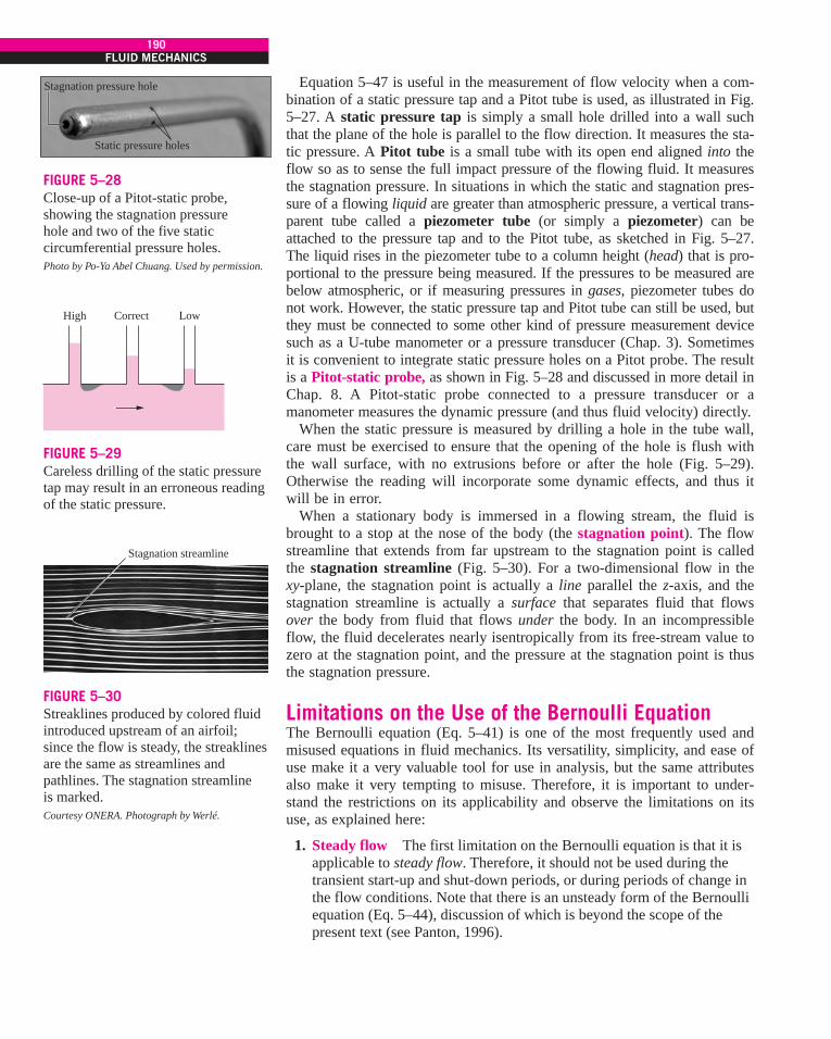
Equation 5–47 is useful in the measurement of flow velocity when a com-bination of a static pressure tap and a Pitot tube is used, as illustrated in Fig.5–27. A static pressure tap is simply a small hole drilled into a wall suchthat the plane of the hole is parallel to the flow direction. It measures the sta-tic pressure. A Pitot tube is a small tube with its open end aligned into theflow so as to sense the full impact pressure of the flowing fluid. It measuresthe stagnation pressure. In situations in which the static and stagnation pres-sure of a flowing liquid are greater than atmospheric pressure, a vertical trans-parent tube called a piezometer tube (or simply a piezometer) can beattached to the pressure tap and to the Pitot tube, as sketched in Fig. 5–27.The liquid rises in the piezometer tube to a column height (head) that is pro-portional to the pressure being measured. If the pressures to be measured arebelow atmospheric, or if measuring pressures in gases, piezometer tubes donot work. However, the static pressure tap and Pitot tube can still be used, butthey must be connected to some other kind of pressure measurement devicesuch as a U-tube manometer or a pressure transducer (Chap. 3). Sometimesit is convenient to integrate static pressure holes on a Pitot probe. The resultis a Pitot-static probe, as shown in Fig. 5–28 and discussed in more detail inChap. 8. A Pitot-static probe connected to a pressure transducer or amanometer measures the dynamic pressure (and thus fluid velocity) directly.

When the static pressure is measured by drilling a hole in the tube wall,care must be exercised to ensure that the opening of the hole is flush withthe wall surface, with no extrusions before or after the hole (Fig. 5–29).Otherwise the reading will incorporate some dynamic effects, and thus itwill be in error.

When a stationary body is immersed in a flowing stream, the fluid isbrought to a stop at the nose of the body (the stagnation point). The flowstreamline that extends from far upstream to the stagnation point is calledthe stagnation streamline (Fig. 5–30). For a two-dimensional flow in thexy-plane, the stagnation point is actually a line parallel the z-axis, and thestagnation streamline is actually a surface that separates fluid that flowsover the body from fluid that flows under the body. In an incompressibleflow, the fluid decelerates nearly isentropically from its free-stream value tozero at the stagnation point, and the pressure at the stagnation point is thusthe stagnation pressure.

Limitations on the Use of the Bernoulli EquationThe Bernoulli equation (Eq. 5–41) is one of the most frequently used andmisused equations in fluid mechanics. Its versatility, simplicity, and ease ofuse make it a very valuable tool for use in analysis, but the same attributesalso make it very tempting to misuse. Therefore, it is important to under-stand the restrictions on its applicability and observe the limitations on itsuse, as explained here:

1. Steady flow The first limitation on the Bernoulli equation is that it isapplicable to steady flow. Therefore, it should not be used during thetransient start-up and shut-down periods, or during periods of change inthe flow conditions. Note that there is an unsteady form of the Bernoulliequation (Eq. 5–44), discussion of which is beyond the scope of thepresent text (see Panton, 1996).

190FLUID MECHANICS

Stagnation pressure hole

Static pressure holes

FIGURE 5–28Close-up of a Pitot-static probe,showing the stagnation pressure hole and two of the five staticcircumferential pressure holes.Photo by Po-Ya Abel Chuang. Used by permission.

High Correct Low

FIGURE 5–29Careless drilling of the static pressuretap may result in an erroneous readingof the static pressure.

Stagnation streamline

FIGURE 5–30Streaklines produced by colored fluidintroduced upstream of an airfoil;since the flow is steady, the streaklinesare the same as streamlines andpathlines. The stagnation streamline is marked.Courtesy ONERA. Photograph by Werlé.

cen72367_ch05.qxd 10/29/04 2:25 PM Page 190

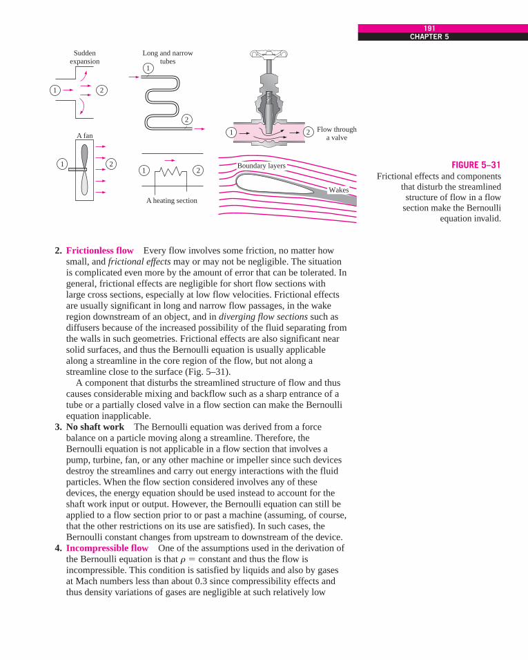
2. Frictionless flow Every flow involves some friction, no matter howsmall, and frictional effects may or may not be negligible. The situationis complicated even more by the amount of error that can be tolerated. Ingeneral, frictional effects are negligible for short flow sections withlarge cross sections, especially at low flow velocities. Frictional effectsare usually significant in long and narrow flow passages, in the wakeregion downstream of an object, and in diverging flow sections such asdiffusers because of the increased possibility of the fluid separating fromthe walls in such geometries. Frictional effects are also significant nearsolid surfaces, and thus the Bernoulli equation is usually applicablealong a streamline in the core region of the flow, but not along astreamline close to the surface (Fig. 5–31).

A component that disturbs the streamlined structure of flow and thuscauses considerable mixing and backflow such as a sharp entrance of atube or a partially closed valve in a flow section can make the Bernoulliequation inapplicable.

3. No shaft work The Bernoulli equation was derived from a forcebalance on a particle moving along a streamline. Therefore, theBernoulli equation is not applicable in a flow section that involves apump, turbine, fan, or any other machine or impeller since such devicesdestroy the streamlines and carry out energy interactions with the fluidparticles. When the flow section considered involves any of thesedevices, the energy equation should be used instead to account for theshaft work input or output. However, the Bernoulli equation can still beapplied to a flow section prior to or past a machine (assuming, of course,that the other restrictions on its use are satisfied). In such cases, theBernoulli constant changes from upstream to downstream of the device.

4. Incompressible flow One of the assumptions used in the derivation ofthe Bernoulli equation is that r ! constant and thus the flow isincompressible. This condition is satisfied by liquids and also by gasesat Mach numbers less than about 0.3 since compressibility effects andthus density variations of gases are negligible at such relatively low

191CHAPTER 5

A fan

Suddenexpansion

Long and narrowtubes

A heating section

Flow througha valve

2

2

2

21

1

1

1

1 2

Boundary layers

Wakes

FIGURE 5–31Frictional effects and components

that disturb the streamlinedstructure of flow in a flow

section make the Bernoulli equation invalid.

cen72367_ch05.qxd 10/29/04 2:25 PM Page 191

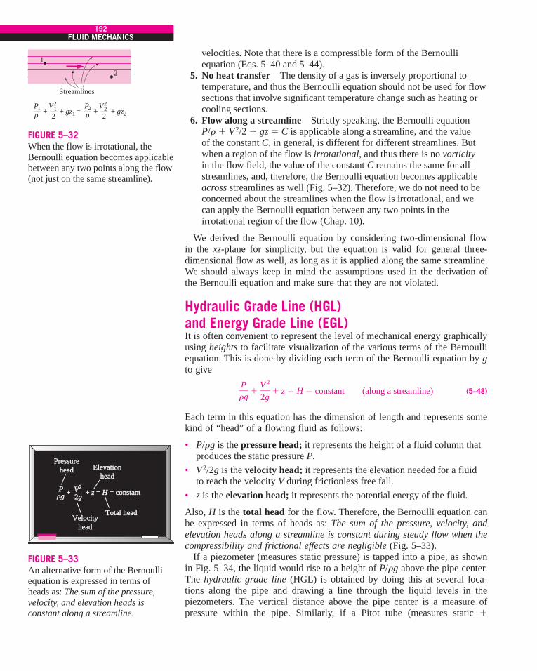
velocities. Note that there is a compressible form of the Bernoulliequation (Eqs. 5–40 and 5–44).

5. No heat transfer The density of a gas is inversely proportional totemperature, and thus the Bernoulli equation should not be used for flowsections that involve significant temperature change such as heating orcooling sections.

6. Flow along a streamline Strictly speaking, the Bernoulli equationP/r ' V2/2 ' gz ! C is applicable along a streamline, and the value of the constant C, in general, is different for different streamlines. Butwhen a region of the flow is irrotational, and thus there is no vorticityin the flow field, the value of the constant C remains the same for allstreamlines, and, therefore, the Bernoulli equation becomes applicableacross streamlines as well (Fig. 5–32). Therefore, we do not need to beconcerned about the streamlines when the flow is irrotational, and wecan apply the Bernoulli equation between any two points in theirrotational region of the flow (Chap. 10).

We derived the Bernoulli equation by considering two-dimensional flowin the xz-plane for simplicity, but the equation is valid for general three-dimensional flow as well, as long as it is applied along the same streamline.We should always keep in mind the assumptions used in the derivation ofthe Bernoulli equation and make sure that they are not violated.

Hydraulic Grade Line (HGL) and Energy Grade Line (EGL)It is often convenient to represent the level of mechanical energy graphicallyusing heights to facilitate visualization of the various terms of the Bernoulliequation. This is done by dividing each term of the Bernoulli equation by gto give

(5–48)

Each term in this equation has the dimension of length and represents somekind of “head” of a flowing fluid as follows:

• P/rg is the pressure head; it represents the height of a fluid column thatproduces the static pressure P.

• V 2/2g is the velocity head; it represents the elevation needed for a fluid to reach the velocity V during frictionless free fall.

• z is the elevation head; it represents the potential energy of the fluid.

Also, H is the total head for the flow. Therefore, the Bernoulli equation canbe expressed in terms of heads as: The sum of the pressure, velocity, andelevation heads along a streamline is constant during steady flow when thecompressibility and frictional effects are negligible (Fig. 5–33).

If a piezometer (measures static pressure) is tapped into a pipe, as shownin Fig. 5–34, the liquid would rise to a height of P/rg above the pipe center.The hydraulic grade line (HGL) is obtained by doing this at several loca-tions along the pipe and drawing a line through the liquid levels in thepiezometers. The vertical distance above the pipe center is a measure ofpressure within the pipe. Similarly, if a Pitot tube (measures static '

Prg

'V 2

2g' z ! H ! constant (along a streamline)

192FLUID MECHANICS

2V2

Streamlines

1

2

+ + gz1 =P1–– ––

2+ + gz2

P2–– ––2rr

1V2

FIGURE 5–32When the flow is irrotational, theBernoulli equation becomes applicablebetween any two points along the flow(not just on the same streamline).

–––– + + + z = = H = constant = constant

PressurePressureheadhead

Pg ––––

2

2g

ElevationElevationheadhead

VelocityVelocityheadhead

Total headTotal head

V r

FIGURE 5–33An alternative form of the Bernoulliequation is expressed in terms ofheads as: The sum of the pressure,velocity, and elevation heads isconstant along a streamline.

cen72367_ch05.qxd 10/29/04 2:25 PM Page 192

dynamic pressure) is tapped into a pipe, the liquid would rise to a height ofP/rg ' V2/2g above the pipe center, or a distance of V2/2g above the HGL.The energy grade line (EGL) is obtained by doing this at several locationsalong the pipe and drawing a line through the liquid levels in the Pitot tubes.

Noting that the fluid also has elevation head z (unless the reference levelis taken to be the centerline of the pipe), the HGL and EGL can be definedas follows: The line that represents the sum of the static pressure and theelevation heads, P/rg ' z, is called the hydraulic grade line. The line thatrepresents the total head of the fluid, P/rg ' V2/2g ' z, is called theenergy grade line. The difference between the heights of EGL and HGL isequal to the dynamic head, V 2/2g. We note the following about the HGLand EGL:

• For stationary bodies such as reservoirs or lakes, the EGL and HGLcoincide with the free surface of the liquid. The elevation of the freesurface z in such cases represents both the EGL and the HGL since thevelocity is zero and the static pressure (gage) is zero.

• The EGL is always a distance V2/2g above the HGL. These two linesapproach each other as the velocity decreases, and they diverge as thevelocity increases. The height of the HGL decreases as the velocityincreases, and vice versa.

• In an idealized Bernoulli-type flow, EGL is horizontal and its heightremains constant. This would also be the case for HGL when the flowvelocity is constant (Fig. 5–35).

• For open-channel flow, the HGL coincides with the free surface of theliquid, and the EGL is a distance V 2/2g above the free surface.

• At a pipe exit, the pressure head is zero (atmospheric pressure) and thusthe HGL coincides with the pipe outlet (location 3 on Fig. 5–34).

• The mechanical energy loss due to frictional effects (conversion tothermal energy) causes the EGL and HGL to slope downward in thedirection of flow. The slope is a measure of the head loss in the pipe(discussed in detail in Chap. 8). A component that generates significantfrictional effects such as a valve causes a sudden drop in both EGL andHGL at that location.

• A steep jump occurs in EGL and HGL whenever mechanical energy isadded to the fluid (by a pump, for example). Likewise, a steep drop

193CHAPTER 5

Diffuser

Arbitrary reference plane (z = 0)

HGL

EGL

1

/2g

z

0

2 3

1

/2g2V2

V2

FIGURE 5–34The hydraulic grade line (HGL) andthe energy grade line (EGL) for freedischarge from a reservoir through a

horizontal pipe with a diffuser.

Reference level0

(Horizontal) EGL

z

HGL

P–– g

2/2gV

r

FIGURE 5–35In an idealized Bernoulli-type flow,

EGL is horizontal and its heightremains constant. But this is not the case for HGL when the flow

velocity varies along the flow.

cen72367_ch05.qxd 10/29/04 2:25 PM Page 193

occurs in EGL and HGL whenever mechanical energy is removed fromthe fluid (by a turbine, for example), as shown in Fig. 5–36.

• The pressure (gage) of a fluid is zero at locations where the HGLintersects the fluid. The pressure in a flow section that lies above the HGLis negative, and the pressure in a section that lies below the HGL ispositive (Fig. 5–37). Therefore, an accurate drawing of a piping systemand the HGL can be used to determine the regions where the pressure inthe pipe is negative (below the atmospheric pressure).

The last remark enables us to avoid situations in which the pressure dropsbelow the vapor pressure of the liquid (which causes cavitation, as dis-cussed in Chap. 2). Proper consideration is necessary in the placement of aliquid pump to ensure that the suction side pressure does not fall too low,especially at elevated temperatures where vapor pressure is higher than it isat low temperatures.

Now we examine Fig. 5–34 more closely. At point 0 (at the liquid surface),EGL and HGL are even with the liquid surface since there is no flow there.HGL decreases rapidly as the liquid accelerates into the pipe; however, EGLdecreases very slowly through the well-rounded pipe inlet. EGL declines con-tinually along the flow direction due to friction and other irreversible losses inthe flow. EGL cannot increase in the flow direction unless energy is suppliedto the fluid. HGL can rise or fall in the flow direction, but can never exceedEGL. HGL rises in the diffuser section as the velocity decreases, and the sta-tic pressure recovers somewhat; the total pressure does not recover, however,and EGL decreases through the diffuser. The difference between EGL andHGL is V2

1/2g at point 1, and V22/2g at point 2. Since V1 & V2, the difference

between the two grade lines is larger at point 1 than at point 2. The downwardslope of both grade lines is larger for the smaller diameter section of pipesince the frictional head loss is greater. Finally, HGL decays to the liquid sur-face at the outlet since the pressure there is atmospheric. However, EGL isstill higher than HGL by the amount V2

2/2g since V3 ! V2 at the outlet.

5–5 ! APPLICATIONS OF THE BERNOULLI EQUATION

In Section 5–4, we discussed the fundamental aspects of the Bernoulli equa-tion. In this section, we demonstrate its use in a wide range of applicationsthrough examples.

EXAMPLE 5–5 Spraying Water into the Air

Water is flowing from a hose attached to a water main at 400 kPa gage (Fig.5–38). A child places his thumb to cover most of the hose outlet, causing athin jet of high-speed water to emerge. If the hose is held upward, what isthe maximum height that the jet could achieve?

SOLUTION Water from a hose attached to the water main is sprayed intothe air. The maximum height the water jet can rise is to be determined.Assumptions 1 The flow exiting into the air is steady, incompressible, andirrotational (so that the Bernoulli equation is applicable). 2 The water pressure

194FLUID MECHANICS

Pump Turbine

EGL

HGL

Wpump Wturbine· ·

FIGURE 5–36A steep jump occurs in EGL and HGLwhenever mechanical energy is addedto the fluid by a pump, and a steep dropoccurs whenever mechanical energy isremoved from the fluid by a turbine.

Negative P

P = 0

P = 0HGL

Positive P

Positive P

FIGURE 5–37The pressure (gage) of a fluid is zeroat locations where the HGL intersectsthe fluid, and the pressure is negative(vacuum) in a flow section that liesabove the HGL.

cen72367_ch05.qxd 10/29/04 2:25 PM Page 194

in the hose near the outlet is equal to the water main pressure. 3 The surfacetension effects are negligible. 4 The friction between the water and air is neg-ligible. 5 The irreversibilities that may occur at the outlet of the hose due toabrupt expansion are negligible.Properties We take the density of water to be 1000 kg/m3.Analysis This problem involves the conversion of flow, kinetic, and potentialenergies to each other without involving any pumps, turbines, and wastefulcomponents with large frictional losses, and thus it is suitable for the use ofthe Bernoulli equation. The water height will be maximum under the statedassumptions. The velocity inside the hose is relatively low (V1 # 0) and wetake the hose outlet as the reference level (z1 ! 0). At the top of the watertrajectory V2 ! 0, and atmospheric pressure pertains. Then the Bernoulliequation simplifies to

Solving for z2 and substituting,

Therefore, the water jet can rise as high as 40.8 m into the sky in this case.Discussion The result obtained by the Bernoulli equation represents theupper limit and should be interpreted accordingly. It tells us that the watercannot possibly rise more than 40.8 m, and, in all likelihood, the rise will bemuch less than 40.8 m due to irreversible losses that we neglected.

EXAMPLE 5–6 Water Discharge from a Large Tank

A large tank open to the atmosphere is filled with water to a height of 5 mfrom the outlet tap (Fig. 5–39). A tap near the bottom of the tank is nowopened, and water flows out from the smooth and rounded outlet. Determinethe water velocity at the outlet.

SOLUTION A tap near the bottom of a tank is opened. The exit velocity ofwater from the tank is to be determined.Assumptions 1 The flow is incompressible and irrotational (except very closeto the walls). 2 The water drains slowly enough that the flow can be approxi-mated as steady (actually quasi-steady when the tank begins to drain).Analysis This problem involves the conversion of flow, kinetic, and potentialenergies to each other without involving any pumps, turbines, and wastefulcomponents with large frictional losses, and thus it is suitable for the use ofthe Bernoulli equation. We take point 1 to be at the free surface of water sothat P1 ! Patm (open to the atmosphere), V1 # 0 (the tank is large relative tothe outlet), and z1 ! 5 m and z2 ! 0 (we take the reference level at thecenter of the outlet). Also, P2 ! Patm (water discharges into the atmosphere).Then the Bernoulli equation simplifies to

P1

rg'

V 21

2g ' z1 !

P2

rg'

V 22

2g' z2 ! z1 !

V 22

2g

! 40.8 m

z2 !P1 " Patm

rg !P1, gage

rg !400 kPa

(1000 kg/m3)(9.81 m/s2) a1000 N/m2

1 kPa b a1 kg ( m/s2

1 N bP1

rg 'V 2

1

2g ' z1 !P2

rg 'V

22

2g ' z2 ! P1

rg !Patm

rg ' z2

195CHAPTER 5

Water jet

2

Hose

0

z

1

FIGURE 5–38Schematic for Example 5–5.

Water5 m

0

z

1

2

V2

FIGURE 5–39Schematic for Example 5–6.

0 0 0Q Q¡

0 0Q¡

cen72367_ch05.qxd 10/29/04 2:25 PM Page 195

Solving for V2 and substituting,

The relation V ! is called the Toricelli equation.Therefore, the water leaves the tank with an initial velocity of 9.9 m/s.

This is the same velocity that would manifest if a solid were dropped a dis-tance of 5 m in the absence of air friction drag. (What would the velocity beif the tap were at the bottom of the tank instead of on the side?)Discussion If the orifice were sharp-edged instead of rounded, then the flowwould be disturbed, and the velocity would be less than 9.9 m/s, especiallynear the edges. Care must be exercised when attempting to apply theBernoulli equation to situations where abrupt expansions or contractionsoccur since the friction and flow disturbance in such cases may not be neg-ligible.

EXAMPLE 5–7 Siphoning Out Gasoline from a Fuel Tank

During a trip to the beach (Patm ! 1 atm ! 101.3 kPa), a car runs out ofgasoline, and it becomes necessary to siphon gas out of the car of a GoodSamaritan (Fig. 5–40). The siphon is a small-diameter hose, and to start thesiphon it is necessary to insert one siphon end in the full gas tank, fill thehose with gasoline via suction, and then place the other end in a gas canbelow the level of the gas tank. The difference in pressure between point 1(at the free surface of the gasoline in the tank) and point 2 (at the outlet ofthe tube) causes the liquid to flow from the higher to the lower elevation.Point 2 is located 0.75 m below point 1 in this case, and point 3 is located2 m above point 1. The siphon diameter is 4 mm, and frictional losses inthe siphon are to be disregarded. Determine (a) the minimum time to with-draw 4 L of gasoline from the tank to the can and (b) the pressure at point3. The density of gasoline is 750 kg/m3.

SOLUTION Gasoline is to be siphoned from a tank. The minimum time ittakes to withdraw 4 L of gasoline and the pressure at the highest point inthe system are to be determined.Assumptions 1 The flow is steady and incompressible. 2 Even though theBernoulli equation is not valid through the pipe because of frictional losses,we employ the Bernoulli equation anyway in order to obtain a best-case esti-mate. 3 The change in the gasoline surface level inside the tank is negligiblecompared to elevations z1 and z2 during the siphoning period.Properties The density of gasoline is given to be 750 kg/m3.Analysis (a) We take point 1 to be at the free surface of gasoline in thetank so that P1 ! Patm (open to the atmosphere), V1 # 0 (the tank is largerelative to the tube diameter), and z2 ! 0 (point 2 is taken as the referencelevel). Also, P2 ! Patm (gasoline discharges into the atmosphere). Then theBernoulli equation simplifies to

Solving for V2 and substituting,

V2 ! 22gz1 ! 22(9.81 m/s2)(0.75 m) ! 3.84 m/s

P1

rg'

V 21

2g ' z1 !

P2

rg'

V 22

2g' z2 ! z1 !

V 22

2g

12gz

V2 ! 22gz1 ! 22(9.81 m/s2)(5 m) ! 9.9 m/s

196FLUID MECHANICS

0 0Q¡

0

z

z3

z1

z2

Gastank

0.75 m

2 m

Gasolinesiphoning

tube

Gas can

1

2

3

FIGURE 5–40Schematic for Example 5–7.

cen72367_ch05.qxd 10/29/04 2:25 PM Page 196

The cross-sectional area of the tube and the flow rate of gasoline are

Then the time needed to siphon 4 L of gasoline becomes

(b) The pressure at point 3 can be determined by writing the Bernoulli equa-tion between points 2 and 3. Noting that V2 ! V3 (conservation of mass), z2! 0, and P2 ! Patm,

Solving for P3 and substituting,

Discussion The siphoning time is determined by neglecting frictionaleffects, and thus this is the minimum time required. In reality, the time willbe longer than 53.1 s because of friction between the gasoline and the tubesurface. Also, the pressure at point 3 is below the atmospheric pressure. Ifthe elevation difference between points 1 and 3 is too high, the pressure atpoint 3 may drop below the vapor pressure of gasoline at the gasoline tem-perature, and some gasoline may evaporate (cavitate). The vapor then mayform a pocket at the top and halt the flow of gasoline.

EXAMPLE 5–8 Velocity Measurement by a Pitot Tube

A piezometer and a Pitot tube are tapped into a horizontal water pipe, asshown in Fig. 5–41, to measure static and stagnation (static ' dynamic)pressures. For the indicated water column heights, determine the velocity atthe center of the pipe.

SOLUTION The static and stagnation pressures in a horizontal pipe aremeasured. The velocity at the center of the pipe is to be determined.Assumptions 1 The flow is steady and incompressible. 2 Points 1 and 2 areclose enough together that the irreversible energy loss between these twopoints is negligible, and thus we can use the Bernoulli equation.Analysis We take points 1 and 2 along the centerline of the pipe, with point1 directly under the piezometer and point 2 at the tip of the Pitot tube. Thisis a steady flow with straight and parallel streamlines, and the gage pres-sures at points 1 and 2 can be expressed as

P2 ! rg(h1 ' h2 ' h3)

P1 ! rg(h1 ' h2)

! 81.1 kPa

! 101.3 kPa " (750 kg/m3)(9.81 m/s2)(2.75 m)a 1 N1 kg ( m/s2b a 1 kPa

1000 N/m2b

P3 ! Patm " rgz3

P2

rg'

V 22

2g' z2 !

P3

rg'

V 23

2g' z3 ! Patm

rg!

P3

rg' z3

$t !V

V# !

4 L0.0753 L/s

! 53.1 s

V#

! V2 A ! (3.84 m/s)(1.96 # 10"5 m2) ! 7.53 # 10"5 m3/s ! 0.0753 L/s

A ! pD2/4 ! p(5 # 10"3 m)2/4 ! 1.96 # 10"5 m2

197CHAPTER 5

¡0

h3 = 12 cm

h2 = 7 cm

h1 = 3 cm

Stagnationpoint

Water1 2

V1

FIGURE 5–41Schematic for Example 5–8.

cen72367_ch05.qxd 10/29/04 2:25 PM Page 197

Noting that point 2 is a stagnation point and thus V2 ! 0 and z1 ! z2, theapplication of the Bernoulli equation between points 1 and 2 gives

Substituting the P1 and P2 expressions gives

Solving for V1 and substituting,

Discussion Note that to determine the flow velocity, all we need is to mea-sure the height of the excess fluid column in the Pitot tube.

EXAMPLE 5–9 The Rise of the Ocean Due to a Hurricane

A hurricane is a tropical storm formed over the ocean by low atmosphericpressures. As a hurricane approaches land, inordinate ocean swells (veryhigh tides) accompany the hurricane. A Class-5 hurricane features winds inexcess of 155 mph, although the wind velocity at the center “eye” is verylow.

Figure 5–42 depicts a hurricane hovering over the ocean swell below. Theatmospheric pressure 200 mi from the eye is 30.0 in Hg (at point 1, gener-ally normal for the ocean) and the winds are calm. The hurricane atmo-spheric pressure at the eye of the storm is 22.0 in Hg. Estimate the oceanswell at (a) the eye of the hurricane at point 3 and (b) point 2, where thewind velocity is 155 mph. Take the density of seawater and mercury to be64 lbm/ft3 and 848 lbm/ft3, respectively, and the density of air at normalsea-level temperature and pressure to be 0.076 lbm/ft3.

SOLUTION A hurricane is moving over the ocean. The amount of oceanswell at the eye and at active regions of the hurricane are to be determined.Assumptions 1 The airflow within the hurricane is steady, incompressible,and irrotational (so that the Bernoulli equation is applicable). (This is cer-tainly a very questionable assumption for a highly turbulent flow, but it is jus-tified in the solution.) 2 The effect of water drifted into the air is negligible.Properties The densities of air at normal conditions, seawater, and mercuryare given to be 0.076 lbm/ft3, 64 lbm/ft3, and 848 lbm/ft3, respectively.Analysis (a) Reduced atmospheric pressure over the water causes the waterto rise. Thus, decreased pressure at point 2 relative to point 1 causes theocean water to rise at point 2. The same is true at point 3, where the storm airvelocity is negligible. The pressure difference given in terms of the mercurycolumn height can be expressed in terms of the seawater column height by

$P ! (rgh)Hg ! (rgh)sw ! hsw !rHg

rsw hHg

V1 ! 22gh3 ! 22(9.81 m/s2)(0.12 m) ! 1.53 m/s

V 21

2g !P2 " P1

rg !rg(h1 ' h2 ' h3) " rg(h1 ' h2)

rg ! h3

P1

rg'

V 21

2g' z1 !

P2

rg'

V 22

2g ' z2 !

V 21

2g!

P2 " P1

rg

198FLUID MECHANICS

0Q

Calmoceanlevel

Ocean

HurricaneEye

1

23

h1h2

A B

FIGURE 5–42Schematic for Example 5–9. Thevertical scale is greatly exaggerated.

cen72367_ch05.qxd 10/29/04 2:25 PM Page 198

Then the pressure difference between points 1 and 3 in terms of the seawa-ter column height becomes

which is equivalent to the storm surge at the eye of the hurricane since thewind velocity there is negligible and there are no dynamic effects.

(b) To determine the additional rise of ocean water at point 2 due to the highwinds at that point, we write the Bernoulli equation between points A and B,which are on top of the points 2 and 3, respectively. Noting that VB # 0 (theeye region of the hurricane is relatively calm) and zA ! zB (both points areon the same horizontal line), the Bernoulli equation simplifies to

Substituting,

where r is the density of air in the hurricane. Noting that the density of anideal gas at constant temperature is proportional to absolute pressure andthe density of air at the normal atmospheric pressure of 14.7 psia # 30 inHg is 0.076 lbm/ft3, the density of air in the hurricane is

Using the relation developed above in part (a), the seawater column heightequivalent to 803 ft of air column height is determined to be

Therefore, the pressure at point 2 is 0.70 ft seawater column lower than thepressure at point 3 due to the high wind velocities, causing the ocean to risean additional 0.70 ft. Then the total storm surge at point 2 becomes

h2 ! h1 ' hdynamic ! 8.83 ' 0.70 ! 9.53 ft

Discussion This problem involves highly turbulent flow and the intensebreakdown of the streamlines, and thus the applicability of the Bernoulliequation in part (b) is questionable. Furthermore, the flow in the eye of thestorm is not irrotational, and the Bernoulli equation constant changes acrossstreamlines (see Chap. 10). The Bernoulli analysis can be thought of as thelimiting, ideal case, and shows that the rise of seawater due to high-velocitywinds cannot be more than 0.70 ft.

The wind power of hurricanes is not the only cause of damage to coastalareas. Ocean flooding and erosion from excessive tides is just as serious, asare high waves generated by the storm turbulence and energy.

hdynamic !rair

rsw hair ! a0.056 lbm/ft3

64 lbm/ft3 b (803 ft) ! 0.70 ft

rair !Pair

Patm air ratm air ! a22 in Hg

30 in Hgb (0.076 lbm/ft3) ! 0.056 lbm/ft3

PB " PA

rg !V 2

A

2g !(155 mph)2

2(32.2 ft/s2) a1.4667 ft/s

1 mph b 2! 803 ft

PA

rg'

V 2A

2g' zA !

PB

rg'

V 2B

2g ' zB !

PB " PA

rg!

V 2A

2g

h1 !rHg

rsw hHg ! a848 lbm/ft3

64 lbm/ft3 b3(30 " 22) in Hg4a 1 ft12 in

b ! 8.83 ft

199CHAPTER 5

0Q

cen72367_ch05.qxd 10/29/04 2:25 PM Page 199

EXAMPLE 5–10 Bernoulli Equation for Compressible Flow

Derive the Bernoulli equation when the compressibility effects are not negli-gible for an ideal gas undergoing (a) an isothermal process and (b) an isen-tropic process.

SOLUTION The Bernoulli equation for compressible flow is to be obtainedfor an ideal gas for isothermal and isentropic processes.Assumptions 1 The flow is steady and frictional effects are negligible. 2 Thefluid is an ideal gas, so the relation P ! rRT is applicable. 3 The specificheats are constant so that P/rk ! constant during an isentropic process.Analysis (a) When the compressibility effects are significant and the flowcannot be assumed to be incompressible, the Bernoulli equation is given byEq. 5–40 as

(1)

The compressibility effects can be properly accounted for by expressing r interms of pressure, and then performing the integration $ dP/r in Eq. 1. Butthis requires a relation between P and r for the process. For the isothermalexpansion or compression of an ideal gas, the integral in Eq. 1 can be per-formed easily by noting that T ! constant and substituting r ! P/RT. Itgives

Substituting into Eq. 1 gives the desired relation,

Isothermal process: (2)

(b) A more practical case of compressible flow is the isentropic flow of idealgases through equipment that involves high-speed fluid flow such as nozzles,diffusers, and the passages between turbine blades. Isentropic (i.e.,reversible and adiabatic) flow is closely approximated by these devices, andit is characterized by the relation P/rk ! C ! constant, where k is the spe-cific heat ratio of the gas. Solving for r from P/rk ! C gives r ! C "1/kP1/k.Performing the integration,

(3)

Substituting, the Bernoulli equation for steady, isentropic, compressible flowof an ideal gas becomes

Isentropic flow: (4a)

or

(4b)

A common practical situation involves the acceleration of a gas from rest(stagnation conditions at state 1) with negligible change in elevation. Inthat case we have z1 ! z2 and V1 ! 0. Noting that r ! P/RT for ideal

a kk " 1bP1

r1'

V 21

2 ' gz1 ! a kk " 1bP2

r2'

V 22

2 ' gz2

a kk # 1bP

R!

V 2

2 ! gz " constant

! dPr

! ! C 1/kP "1/k dP ! C 1/k P"1/k'1

"1/k ' 1 !P 1/k

r P"1/k'1

"1/k ' 1 ! a kk " 1bP

r

RT ln P !V 2

2 ! gz " constant

! dPr

! ! dPP/RT ! RT ln P

! dPr

'V 2

2 ' gz ! constant (along a streamline)

200FLUID MECHANICS

cen72367_ch05.qxd 10/29/04 2:25 PM Page 200

gases, P/rk ! constant for isentropic flow, and the Mach number is definedas Ma ! V/c where is the local speed of sound for ideal gases,Eq. 4b simplifies to

(4c)

where state 1 is the stagnation state and state 2 is any state along the flow.Discussion It can be shown that the results obtained using the compress-ible and incompressible equations deviate no more than 2 percent when theMach number is less than 0.3. Therefore, the flow of an ideal gas can beconsidered to be incompressible when Ma + 0.3. For atmospheric air at normal conditions, this corresponds to a flow speed of about 100 m/s or 360 km/h, which covers our range of interest.

5–6 ! GENERAL ENERGY EQUATIONOne of the most fundamental laws in nature is the first law of thermody-namics, also known as the conservation of energy principle, which pro-vides a sound basis for studying the relationships among the various formsof energy and energy interactions. It states that energy can be neither cre-ated nor destroyed during a process; it can only change forms. Therefore,every bit of energy must be accounted for during a process.

A rock falling off a cliff, for example, picks up speed as a result of itspotential energy being converted to kinetic energy (Fig. 5–43). Experimen-tal data show that the decrease in potential energy equals the increase inkinetic energy when the air resistance is negligible, thus confirming the con-servation of energy principle. The conservation of energy principle alsoforms the backbone of the diet industry: a person who has a greater energyinput (food) than energy output (exercise) will gain weight (store energy inthe form of fat), and a person who has a smaller energy input than outputwill lose weight. The change in the energy content of a system is equal tothe difference between the energy input and the energy output, and the conservation of energy principle for any system can be expressed simply asEin " Eout ! $E.

The transfer of any quantity (such as mass, momentum, and energy) isrecognized at the boundary as the quantity crosses the boundary. A quantityis said to enter a system if it crosses the boundary from the outside to theinside, and to exit the system if it moves in the reverse direction. A quantitythat moves from one location to another within a system is not consideredas a transferred quantity in an analysis since it does not enter or exit the sys-tem. Therefore, it is important to specify the system and thus clearly iden-tify its boundaries before an engineering analysis is performed.

The energy content of a fixed quantity of mass (a closed system) can bechanged by two mechanisms: heat transfer Q and work transfer W. Then theconservation of energy for a fixed quantity of mass can be expressed in rateform as (Fig. 5–44)

(5–49)Q#net in ' W

#net in !

dE sys

dt or Q

#net in ' W

#net in !

ddt

!sys

re dV

P1

P2! c1 ' ak " 1

2 b Ma 22d k /(k"1)

c ! 1kRT

201CHAPTER 5

PE1 = 10 kJm

KE1 = 0

PE2 = 7 kJm KE2 = 3 kJ

" z

FIGURE 5–43Energy cannot be created or destroyed during a process;

it can only change forms.

Wshaft, in = 6 kJ

= 18 kJ

Qout = 3 kJ

Qin = 15 kJ

"E = (15 – 3) + 6

FIGURE 5–44The energy change of a system

during a process is equal to the network and heat transfer between the

system and its surroundings.

cen72367_ch05.qxd 10/29/04 2:25 PM Page 201

where Q·net in ! Q· in " Q·out is the net rate of heat transfer to the system (neg-ative, if from the system), W

·net in ! W

·in " W

·out is the net power input to the

system in all forms (negative, if power output) and dEsys/dt is the rate ofchange of the total energy content of the system. The overdot stands fortime rate. For simple compressible systems, total energy consists of internal,kinetic, and potential energies, and it is expressed on a unit-mass basis as(see Chap. 2)

(5–50)

Note that total energy is a property, and its value does not change unless thestate of the system changes.

Energy Transfer by Heat, QIn daily life, we frequently refer to the sensible and latent forms of internalenergy as heat, and talk about the heat content of bodies. Scientifically themore correct name for these forms of energy is thermal energy. For single-phase substances, a change in the thermal energy of a given mass results ina change in temperature, and thus temperature is a good representative ofthermal energy. Thermal energy tends to move naturally in the direction ofdecreasing temperature, and the transfer of thermal energy from one systemto another as a result of a temperature difference is called heat transfer.Therefore, an energy interaction is heat transfer only if it takes placebecause of a temperature difference. The warming up of a canned drink in awarmer room, for example, is due to heat transfer (Fig. 5–45). The time rateof heat transfer is called heat transfer rate and is denoted by Q

..

The direction of heat transfer is always from the higher-temperature bodyto the lower-temperature one. Once temperature equality is established, heattransfer stops. There cannot be any heat transfer between two systems (or asystem and its surroundings) that are at the same temperature.

A process during which there is no heat transfer is called an adiabaticprocess. There are two ways a process can be adiabatic: Either the system iswell insulated so that only a negligible amount of heat can pass through thesystem boundary, or both the system and the surroundings are at the sametemperature and therefore there is no driving force (temperature difference)for heat transfer. An adiabatic process should not be confused with anisothermal process. Even though there is no heat transfer during an adia-batic process, the energy content and thus the temperature of a system canstill be changed by other means such as work transfer.

Energy Transfer by Work, WAn energy interaction is work if it is associated with a force acting througha distance. A rising piston, a rotating shaft, and an electric wire crossing thesystem boundary are all associated with work interactions. The time rate ofdoing work is called power and is denoted by W

.. Car engines and hydraulic,

steam, and gas turbines produce work; compressors, pumps, fans, and mix-ers consume work.

Work-consuming devices transfer energy to the fluid, and thus increasethe energy of the fluid. A fan in a room, for example, mobilizes the air andincreases its kinetic energy. The electric energy a fan consumes is first con-verted to mechanical energy by its motor that forces the shaft of the blades

e ! u ' ke ' pe ! u 'V 2

2' gz

202FLUID MECHANICS

Room air25°C

No heattransfer Heat Heat

25°C 5°C

8 J/s 16 J/s

15°C

FIGURE 5–45Temperature difference is the drivingforce for heat transfer. The larger thetemperature difference, the higher isthe rate of heat transfer.

cen72367_ch05.qxd 10/29/04 2:25 PM Page 202

to rotate. This mechanical energy is then transferred to the air, as evidencedby the increase in air velocity. This energy transfer to air has nothing to dowith a temperature difference, so it cannot be heat transfer. Therefore, itmust be work. Air discharged by the fan eventually comes to a stop and thusloses its mechanical energy as a result of friction between air particles ofdifferent velocities. But this is not a “loss” in the real sense; it is simply theconversion of mechanical energy to an equivalent amount of thermal energy(which is of limited value, and thus the term loss) in accordance with theconservation of energy principle. If a fan runs a long time in a sealed room,we can sense the buildup of this thermal energy by a rise in air temperature.

A system may involve numerous forms of work, and the total work can beexpressed as

(5–51)

where Wshaft is the work transmitted by a rotating shaft, Wpressure is the workdone by the pressure forces on the control surface, Wviscous is the work doneby the normal and shear components of viscous forces on the control sur-face, and Wother is the work done by other forces such as electric, magnetic,and surface tension, which are insignificant for simple compressible systemsand are not considered in this text. We do not consider Wviscous either since itis usually small relative to other terms in control volume analysis. But itshould be kept in mind that the work done by shear forces as the bladesshear through the fluid may need to be considered in a refined analysis ofturbomachinery.

Shaft WorkMany flow systems involve a machine such as a pump, a turbine, a fan, or acompressor whose shaft protrudes through the control surface, and the worktransfer associated with all such devices is simply referred to as shaft workWshaft. The power transmitted via a rotating shaft is proportional to the shafttorque Tshaft and is expressed as

(5–52)

where v is the angular speed of the shaft in rad/s and n. is defined as thenumber of revolutions of the shaft per unit time, often expressed in rev/minor rpm.

Work Done by Pressure ForcesConsider a gas being compressed in the piston-cylinder device shown inFig. 5–46a. When the piston moves down a differential distance ds underthe influence of the pressure force PA, where A is the cross-sectional area ofthe piston, the boundary work done on the system is dWboundary ! PA ds.Dividing both sides of this relation by the differential time interval dt givesthe time rate of boundary work (i.e., power),

where Vpiston ! ds/dt is the piston velocity, which is the velocity of the mov-ing boundary at the piston face.

Now consider a material chunk of fluid (a system) of arbitrary shape,which moves with the flow and is free to deform under the influence ofpressure, as shown in Fig. 5–46b. Pressure always acts inward and normal

dW#pressure ! dW

#boundary ! PAVpiston

W#

shaft ! vTshaft ! 2pn#Tshaft

Wtotal ! Wshaft ' Wpressure ' Wviscous ' Wother

203CHAPTER 5

System

System boundary, A

dV

dmdA

P n

u

!V

!

(b)

(a)

ds

P

A

Vpiston

System(gas in cylinder)

FIGURE 5–46The pressure force acting on (a) the

moving boundary of a system in a piston-cylinder device, and

(b) the differential surface area of a system of arbitrary shape.

cen72367_ch05.qxd 10/29/04 2:25 PM Page 203

to the surface, and the pressure force acting on a differential area dA isP dA. Again noting that work is force times distance and distance traveledper unit time is velocity, the time rate at which work is done by pressureforces on this differential part of the system is

(5–53)

since the normal component of velocity through the differential area dA isVn ! V cos u ! V

!· n!. Note that n! is the outer normal of dA, and thus the

quantity V!

· n! is positive for expansion and negative for compression. Thenegative sign in Eq. 5–53 ensures that work done by pressure forces is posi-tive when it is done on the system, and negative when it is done by the sys-tem, which agrees with our sign convention. The total rate of work done bypressure forces is obtained by integrating dW

.pressure over the entire surface A,

(5–54)

In light of these discussions, the net power transfer can be expressed as

(5–55)

Then the rate form of the conservation of energy relation for a closed sys-tem becomes

(5–56)

To obtain a relation for the conservation of energy for a control volume,we apply the Reynolds transport theorem by replacing B with total energyE, and b with total energy per unit mass e, which is e ! u ' ke ' pe ! u' V2/2 ' gz (Fig. 5–47). This yields

(5–57)

Substituting the left-hand side of Eq. 5–56 into Eq. 5–57, the general formof the energy equation that applies to fixed, moving, or deforming controlvolumes becomes

(5–58)

which can be stated as

Here V!

r ! V!

" V!

CS is the fluid velocity relative to the control surface, andthe product r(V

!

r · n!) dA represents the mass flow rate through area elementdA into or out of the control volume. Again noting that n! is the outer normalof dA, the quantity V

!

r · n! and thus mass flow is positive for outflow andnegative for inflow.

§The net rate of energytransfer into a CV by

heat and work transfer¥ ! § The time rate of

change of the energycontent of the CV

¥ ' § The net flow rate ofenergy out of the control

surface by mass flow¥

Q#net in ' W

#shaft, net in ' W

#pressure, net in !

ddt

!CV

er dV ' !CS

er(V!

r ( n!) dA

dE sys

dt!

ddt

!CV

er dV ' !CS

er(V!

r ( n!)A

Q#net in ' W

#shaft, net in ' W

#pressure, net in !

dE sys

dt

W#

net in ! W#

shaft, net in ' W#

pressure, net in ! W#

shaft, net in " !A P(V

!( n

!) dA

W#

pressure, net in ! " !A

P(V!

( n!) dA ! " !

A

Pr

r(V!

( n!) dA

dW#

pressure ! "P dA Vn ! "P dA(V!

( n!)

204FLUID MECHANICS

= +br dV

B = E b = e b = e

dBsys

dtV

d

dtCV! br( r · n ) dA

CS!

= +er dVdEsys

dtV

d

dtCV! er( r · n ) dA

CS!

!

!!

FIGURE 5–47The conservation of energy equation is obtained by replacing B in theReynolds transport theorem by energy E and b by e.

cen72367_ch05.qxd 10/29/04 2:25 PM Page 204

Substituting the surface integral for the rate of pressure work from Eq. 5–54into Eq. 5–58 and combining it with the surface integral on the right give

(5–59)

This is a very convenient form for the energy equation since pressure workis now combined with the energy of the fluid crossing the control surfaceand we no longer have to deal with pressure work.

The term P/r ! Pv ! wflow is the flow work, which is the work associ-ated with pushing a fluid into or out of a control volume per unit mass. Notethat the fluid velocity at a solid surface is equal to the velocity of the solidsurface because of the no-slip condition and is zero for nonmoving surfaces.As a result, the pressure work along the portions of the control surface thatcoincide with nonmoving solid surfaces is zero. Therefore, pressure workfor fixed control volumes can exist only along the imaginary part of thecontrol surface where the fluid enters and leaves the control volume, i.e.,inlets and outlets.

For a fixed control volume (no motion or deformation of control volume),V!

r ! V!

and the energy equation Eq. 5–59 becomes

Fixed CV: (5–60)

This equation is not in a convenient form for solving practical engineeringproblems because of the integrals, and thus it is desirable to rewrite it interms of average velocities and mass flow rates through inlets and outlets. IfP/r ' e is nearly uniform across an inlet or outlet, we can simply take it

outside the integral. Noting that is the mass flow rate

across an inlet or outlet, the rate of inflow or outflow of energy through theinlet or outlet can be approximated as m. (P/r ' e). Then the energy equa-tion becomes (Fig. 5–48)

(5–61)

where e ! u ' V2/2 ' gz (Eq. 5–50) is the total energy per unit mass forboth the control volume and flow streams. Then,

Q#net in ' W

#shaft, net in !

ddt

!CV

er dV ' aout

m# aPr

' eb " ain

m# aPr

' eb

m#

! !Ac

r(V!

( n!) dAc

Q#net in ' W

#shaft, net in !

ddt

!CV

er dV ' !CS

aPr

' ebr(V! ( n!) dA

Q#net in ' W

#shaft, net in !

ddt

!CV

er dV ' !CS

aPr

' ebr(V!r ( n!) dA

205CHAPTER 5

Wshaft, net in

mout ,energyout

energyout

*min ,energyin

*

min ,energyin

*

mout ,*

energyout

mout ,*

*

Qnet in*

In

In

Out

Out

Out

Fixedcontrolvolume

FIGURE 5–48In a typical engineering problem, the

control volume may contain manyinlets and outlets; energy flows in at

each inlet, and energy flows out ateach outlet. Energy also enters the

control volume through net heattransfer and net shaft work.

(5–62)

or

(5–63)

Q#net in ' W

#shaft, net in !

ddt

!CV

er dV ' aout

m# ah '

V 2

2' gzb " a

inm# ah '

V 2

2' gzb

Q#net in ' W

#shaft, net in !

ddt

!CV

er dV ' aout

m# aPr

' u 'V 2

2' gzb " a

inm# aPr

' u 'V2

2' gzb

where we used the definition of enthalpy h ! u ' Pv ! u ' P/r. The lasttwo equations are fairly general expressions of conservation of energy, buttheir use is still limited to fixed control volumes, uniform flow at inlets and

cen72367_ch05.qxd 10/29/04 2:25 PM Page 205

outlets, and negligible work due to viscous forces and other effects. Also,the subscript “net in” stands for “net input,” and thus any heat or worktransfer is positive if to the system and negative if from the system.

5–7 ! ENERGY ANALYSIS OF STEADY FLOWS For steady flows, the time rate of change of the energy content of the con-trol volume is zero, and Eq. 5–63 simplifies to

(5–64)

It states that the net rate of energy transfer to a control volume by heat andwork transfers during steady flow is equal to the difference between therates of outgoing and incoming energy flows with mass.

Many practical problems involve just one inlet and one outlet (Fig. 5–49).The mass flow rate for such single-stream devices remains constant, andEq. 5–64 reduces to

(5–65)

where subscripts 1 and 2 stand for inlet and outlet, respectively. The steady-flow energy equation on a unit-mass basis is obtained by dividing Eq. 5–65by the mass flow rate m. ,

(5–66)

where qnet in ! Q.net in/m

. is the net heat transfer to the fluid per unit mass andwshaft, net in ! W

.shaft, net in/m

. is the net shaft work input to the fluid per unitmass. Using the definition of enthalpy h ! u ' P/r and rearranging, thesteady-flow energy equation can also be expressed as

(5–67)

where u is the internal energy, P/r is the flow energy, V2/2 is the kineticenergy, and gz is the potential energy of the fluid, all per unit mass. Theserelations are valid for both compressible and incompressible flows.

The left side of Eq. 5–67 represents the mechanical energy input, whilethe first three terms on the right side represent the mechanical energy out-put. If the flow is ideal with no irreversibilities such as friction, the totalmechanical energy must be conserved, and the term in parentheses (u2 " u1" qnet in) must equal zero. That is,

Ideal flow (no mechanical energy loss): (5–68)

Any increase in u2 " u1 above qnet in is due to the irreversible conversion ofmechanical energy to thermal energy, and thus u2 " u1 " qnet in representsthe mechanical energy loss (Fig. 5–50). That is,

Mechanical energy loss: (5–69)

For single-phase fluids (a gas or a liquid), we have u2 " u1 ! cv(T2 " T1)where cv is the constant-volume specific heat.

emech, loss ! u2 " u1 " qnet in

qnet in ! u2 " u1

wshaft, net in 'P1

r1'

V 21

2' gz1 !

P2

r2'

V 22

2' gz2 ' (u2 " u1 " qnet in)

qnet in ' wshaft, net in ! h2 " h1 'V 2

2 " V 21

2' g(z2 " z1)

Q#net in ' W

#shaft, net in ! m

# ah2 " h1 'V 2

2 " V 21

2' g(z2 " z1)b

Q#net in ' W

#shaft, net in ! a

outm# ah '

V 2

2' gzb " a

inm# ah '

V 2

2' gzb

206FLUID MECHANICS

+ + h1

Qnet in + Wshaft, net in

gz121m*

* *

2V

In

Out

Fixedcontrolvolume

2

1

+ + h2 gz222m*2V

Q Q

Q Q

FIGURE 5–49A control volume with only one inletand one outlet and energy interactions.

15.2°C

15.0°C

Water

0.7 kg/s

"u = 0.84 kJ/kg"T = 0.2°C

2 kW pump = 0.70h

FIGURE 5–50The lost mechanical energy in a fluidflow system results in an increase inthe internal energy of the fluid andthus in a rise of fluid temperature.

cen72367_ch05.qxd 10/29/04 2:25 PM Page 206

The steady-flow energy equation on a unit-mass basis can be written con-veniently as a mechanical energy balance as

(5–70)

or

(5–71)

Noting that wshaft, net in ! wshaft, in " wshaft, out ! wpump " wturbine, the mechan-ical energy balance can be written more explicitly as

(5–72)

where wpump is the mechanical work input (due to the presence of a pump,fan, compressor, etc.) and wturbine is the mechanical work output. When theflow is incompressible, either absolute or gage pressure can be used for Psince Patm/r would appear on both sides and would cancel out.

Multiplying Eq. 5–72 by the mass flow rate m. gives

(5–73)

where W.pump is the shaft power input through the pump’s shaft, W

.turbine is the

shaft power output through the turbine’s shaft, and E.mech, loss is the total

mechanical power loss, which consists of pump and turbine losses as well asthe frictional losses in the piping network. That is,

E.mech, loss ! E

.mech loss, pump ' E

.mech loss, turbine ' E

.mech loss, piping

By convention, irreversible pump and turbine losses are treated separatelyfrom irreversible losses due to other components of the piping system. Thusthe energy equation can be expressed in its most common form in terms ofheads as (Fig. 5–51).

(5–74)

where is the useful head deliv-

ered to the fluid by the pump. Because of irreversible losses in the pump,hpump, u is less than W

.pump/m

.g by the factor hpump. Similarly,

is the extracted head removed

from the fluid by the turbine. Because of irreversible losses in the turbine,hturbine, e is greater than W

.turbine/m

.g by the factor hturbine. Finally,

is the irreversible head loss between

1 and 2 due to all components of the piping system other than the pump orturbine. Note that the head loss hL represents the frictional losses associatedwith fluid flow in piping, and it does not include the losses that occur withinthe pump or turbine due to the inefficiencies of these devices—these lossesare taken into account by hpump and hturbine. Equation 5–74 is illustratedschematically in Fig. 5–51.

hL !emech loss, piping

g!

E#mech loss, piping

m#g

hturbine, e !wturbine, e

g!

W#

turbine, e

m#g

!W#

turbine

hturbinem#g

hpump, u !wpump, u

g!

W#

pump, u

m#g

!hpumpW

#pump

m#g

P1

r1g'

V 21

2g' z1 ' hpump, u !

P2

r2g'

V 22

2g' z2 ' hturbine, e ' hL

m# aP1

r1'

V 21

2' gz1b ' W

#pump ! m

# aP2

r2'

V 22

2' gz2b ' W

#turbine ' E

#mech, loss

P1

r1'

V 21

2' gz1 ' wpump !

P2

r2'

V 22

2' gz2 ' wturbine ' emech, loss

wshaft, net in 'P1

r1'

V 21

2' gz1 !

P2

r2'

V 22

2' gz2 ' emech, loss

emech, in ! emech, out ' emech, loss

207CHAPTER 5

cen72367_ch05.qxd 10/29/04 2:25 PM Page 207

The pump head is zero if the piping system does not involve a pump, afan, or a compressor, and the turbine head is zero if the system does notinvolve a turbine. Also, the head loss hL can sometimes be ignored when thefrictional losses in the piping system are negligibly small compared to theother terms in Eq. 5–74.

Special Case: Incompressible Flow with NoMechanical Work Devices and Negligible FrictionWhen piping losses are negligible, there is negligible dissipation of mechan-ical energy into thermal energy, and thus hL ! emech loss, piping /g + 0, as shownlater in Example 5–11. Also, hpump, u ! hturbine, e ! 0 when there are nomechanical work devices such as fans, pumps, or turbines. Then Eq. 5–74reduces to

(5–75)

which is the Bernoulli equation derived earlier using Newton’s second lawof motion.

Kinetic Energy Correction Factor, AThe average flow velocity Vavg was defined such that the relation rVavgA givesthe actual mass flow rate. Therefore, there is no such thing as a correction fac-tor for mass flow rate. However, as Gaspard Coriolis (1792–1843) showed,the kinetic energy of a fluid stream obtained from V2/2 is not the same as theactual kinetic energy of the fluid stream since the square of a sum is not equalto the sum of the squares of its components (Fig. 5–52). This error can be cor-rected by replacing the kinetic energy terms V2/2 in the energy equation byaV avg

2 /2, where a is the kinetic energy correction factor. By using equationsfor the variation of velocity with the radial distance, it can be shown that thecorrection factor is 2.0 for fully developed laminar pipe flow, and it rangesbetween 1.04 and 1.11 for fully developed turbulent flow in a round pipe.

The kinetic energy correction factors are often ignored (i.e., a is set equalto 1) in an elementary analysis since (1) most flows encountered in practiceare turbulent, for which the correction factor is near unity, and (2) the

P1

rg'

V 21

2g' z1 !

P2

rg'

V 22

2g' z2 or P

rg'

V 2

2g' z ! constant

208FLUID MECHANICS

Control volume

Emech loss, pump·

Wpump, u·

Wpump·

hpump, u

hturbine, e

Emech fluid, out·

Wturbine, e·

Wturbine·

Emech loss, turbine

·

hL

P1 z1

rg+ +

2g rg

P2 z2 + +

2g

Emech loss, piping·

2V2 1V2 Emech fluid, in·

FIGURE 5–51Mechanical energy flow chart for a fluid flow system that involves a pump and a turbine. Verticaldimensions show each energy termexpressed as an equivalent columnheight of fluid, i.e., head,corresponding to each term of Eq. 5–74.

cen72367_ch05.qxd 10/29/04 2:25 PM Page 208

kinetic energy terms are often small relative to the other terms in the energyequation, and multiplying them by a factor less than 2.0 does not makemuch difference. Besides, when the velocity and thus the kinetic energy arehigh, the flow turns turbulent. However, you should keep in mind that youmay encounter some situations for which these factors are significant, espe-cially when the flow is laminar. Therefore, we recommend that you alwaysinclude the kinetic energy correction factor when analyzing fluid flow prob-lems. When the kinetic energy correction factors are included, the energyequations for steady incompressible flow (Eqs. 5–73 and 5–74) become

(5–76)

(5–77)

If the flow at an inlet or outlet is fully developed turbulent pipe flow, werecommend using a ! 1.05 as a reasonable estimate of the correction fac-tor. This leads to a more conservative estimate of head loss, and it does nottake much additional effort to include a in the equations.

EXAMPLE 5–11 Effect of Friction on Fluid Temperature and Head Loss

Show that during steady and incompressible flow of a fluid in an adiabaticflow section (a) the temperature remains constant and there is no head losswhen friction is ignored and (b) the temperature increases and some headloss occurs when frictional effects are considered. Discuss if it is possible forthe fluid temperature to decrease during such flow (Fig. 5–53).

SOLUTION Steady and incompressible flow through an adiabatic section isconsidered. The effects of friction on the temperature and the heat loss areto be determined.Assumptions 1 The flow is steady and incompressible. 2 The flow section isadiabatic and thus there is no heat transfer, qnet in ! 0.Analysis The density of a fluid remains constant during incompressible flowand the entropy change is

This relation represents the entropy change of the fluid per unit mass as itflows through the flow section from state 1 at the inlet to state 2 at theoutlet. Entropy change is caused by two effects: (1) heat transfer and(2) irreversibilities. Therefore, in the absence of heat transfer, entropy changeis due to irreversibilities only, whose effect is always to increase entropy.

(a) The entropy change of the fluid in an adiabatic flow section (qnet in ! 0)is zero when the process does not involve any irreversibilities such as frictionand swirling, and thus for reversible flow we have

Temperature change: $s ! cv ln T2

T1! 0 ! T2 ! T1

$s ! cv ln T2

T1

P1

rg' a1

V 12

2g' z1 ' hpump, u !

P2

rg' a2

V 22

2g' z2 ' hturbine, e ' hL

m# aP1

r' a1

V 12

2' gz1b ' W

#pump ! m

# aP2

r' a2

V 22

2' gz2b ' W

#turbine ' E

#mech, loss

209CHAPTER 5

1 2T1u1

T2u2

= constant(

(adiabatic)

FIGURE 5–53Schematic for Example 5–11.

KEact = !!kedm = !!A

!!A

V2 (r)[rV(r) dA]· ·

·

m = rVavg A, r = constant

V(r) A

·

––12

rAV3––12

KEavg = avg avg=mV2· ––12

KEacta = =

3

dA·

KEavg· ––––––––

V(r)Vavg––––1

A

r !!AV3(r) dA= ––12

a bFIGURE 5–52

The determination of the kineticenergy correction factor using actual

velocity distribution V(r) and theaverage velocity Vavg at a cross section.

cen72367_ch05.qxd 10/29/04 2:25 PM Page 209

Mechanical energy loss:

Head loss:

Thus we conclude that when heat transfer and frictional effects are negligi-ble, (1) the temperature of the fluid remains constant, (2) no mechanicalenergy is converted to thermal energy, and (3) there is no irreversible headloss.

(b) When irreversibilities such as friction are taken into account, the entropychange is positive and thus we have:

Temperature change:

Mechanical energy loss:

Head loss:

Thus we conclude that when the flow is adiabatic and irreversible, (1) thetemperature of the fluid increases, (2) some mechanical energy is convertedto thermal energy, and (3) some irreversible head loss occurs.Discussion It is impossible for the fluid temperature to decrease duringsteady, incompressible, adiabatic flow since this would require the entropy ofan adiabatic system to decrease, which would be a violation of the secondlaw of thermodynamics.

EXAMPLE 5–12 Pumping Power and Frictional Heating in a Pump

The pump of a water distribution system is powered by a 15-kW electricmotor whose efficiency is 90 percent (Fig. 5–54). The water flow ratethrough the pump is 50 L/s. The diameters of the inlet and outlet pipes arethe same, and the elevation difference across the pump is negligible. If thepressures at the inlet and outlet of the pump are measured to be 100 kPaand 300 kPa (absolute), respectively, determine (a) the mechanical effi-ciency of the pump and (b) the temperature rise of water as it flows throughthe pump due to the mechanical inefficiency.

SOLUTION The pressures across a pump are measured. The mechanicalefficiency of the pump and the temperature rise of water are to be deter-mined.Assumptions 1 The flow is steady and incompressible. 2 The pump is drivenby an external motor so that the heat generated by the motor is dissipated tothe atmosphere. 3 The elevation difference between the inlet and outlet ofthe pump is negligible, z1 # z2. 4 The inlet and outlet diameters are thesame and thus the inlet and outlet velocities and kinetic energy correctionfactors are equal, V1 ! V2 and a1 ! a2.Properties We take the density of water to be 1 kg/L ! 1000 kg/m3 and itsspecific heat to be 4.18 kJ/kg · °C.Analysis (a) The mass flow rate of water through the pump is

m#

! rV#

! (1 kg/L)(50 L/s) ! 50 kg/s

hL ! emech loss, piping/g & 0

emech loss, piping ! u2 " u1 " qnet in ! cv(T2 " T1) & 0

$s ! cv ln T2

T1& 0 ! T2 & T1

hL ! emech loss, piping/g ! 0

emech loss, piping ! u2 " u1 " qnet in ! cv(T2 " T1) " qnet in ! 0

210FLUID MECHANICS

300 kPa

Water

Motor15 kW

motor = 90%,

50 L/s

100 kPa1

2

Wpump·

FIGURE 5–54Schematic for Example 5–12.

cen72367_ch05.qxd 10/29/04 2:25 PM Page 210

The motor draws 15 kW of power and is 90 percent efficient. Thus themechanical (shaft) power it delivers to the pump is

To determine the mechanical efficiency of the pump, we need to know theincrease in the mechanical energy of the fluid as it flows through the pump,which is

Simplifying it for this case and substituting the given values,

Then the mechanical efficiency of the pump becomes

(b) Of the 13.5-kW mechanical power supplied by the pump, only 10 kW isimparted to the fluid as mechanical energy. The remaining 3.5 kW is con-verted to thermal energy due to frictional effects, and this “lost” mechanicalenergy manifests itself as a heating effect in the fluid,

The temperature rise of water due to this mechanical inefficiency is deter-mined from the thermal energy balance, E

.mech, loss ! m

.(u2 " u1) ! m

.c$T.

Solving for $T,

Therefore, the water will experience a temperature rise of 0.017°C due tomechanical inefficiency, which is very small, as it flows through the pump.Discussion In an actual application, the temperature rise of water will prob-ably be less since part of the heat generated will be transferred to the casingof the pump and from the casing to the surrounding air. If the entire pumpmotor were submerged in water, then the 1.5 kW dissipated to the air due tomotor inefficiency would also be transferred to the surrounding water asheat. This would cause the water temperature to rise more.

EXAMPLE 5–13 Hydroelectric Power Generation from a Dam

In a hydroelectric power plant, 100 m3/s of water flows from an elevation of120 m to a turbine, where electric power is generated (Fig. 5–55). The totalirreversible head loss in the piping system from point 1 to point 2 (excludingthe turbine unit) is determined to be 35 m. If the overall efficiency of theturbine–generator is 80 percent, estimate the electric power output.

SOLUTION The available head, flow rate, head loss, and efficiency of ahydroelectric turbine are given. The electric power output is to be determined.Assumptions 1 The flow is steady and incompressible. 2 Water levels at thereservoir and the discharge site remain constant.Properties We take the density of water to be 1000 kg/m3.

$T !E#

mech, loss

m#c

!3.5 kW

(50 kg/s)(4.18 kJ/ kg ( ,C)! 0.017,C

E#

mech, loss ! W#

pump, shaft " $E#

mech, fluid ! 13.5 " 10 ! 3.5 kW

hpump !W#

pump, u

W#

pump, shaft!

$E#

mech, fluid

W#

pump, shaft

!10 kW

13.5 kW! 0.741 or 74.1%

$E#

mech, fluid ! m# aP2 " P1

rb ! (50 kg/s)a(300 " 100) kPa

1000 kg/m3 b a 1 kJ1 kPa ( m3b ! 10 kW

$E#

mech, fluid ! E#

mech, out " E#

mech, in ! m# aP2

r' a2

V 22

2 ' gz2b " m# aP1

r' a1

V 21

2 ' gz1bW#

pump, shaft ! hmotorW#

electric ! (0.90)(15 kW) ! 13.5 kW

211CHAPTER 5

hturbine–gen = 80%

100 m3/s

hL = 35 m

2

120 m

1

Generator

Turbine

FIGURE 5–55Schematic for Example 5–13.

cen72367_ch05.qxd 10/29/04 2:25 PM Page 211

Analysis The mass flow rate of water through the turbine is

We take point 2 as the reference level, and thus z2 ! 0. Also, both points 1and 2 are open to the atmosphere (P1 ! P2 ! Patm) and the flow velocitiesare negligible at both points (V1 ! V2 ! 0). Then the energy equation forsteady, incompressible flow reduces to

Substituting, the extracted turbine head and the corresponding turbinepower are

hturbine, e ! z1 " hL ! 120 " 35 ! 85 m

Therefore, a perfect turbine–generator would generate 83,400 kW of elec-tricity from this resource. The electric power generated by the actual unit is

W.

electric ! hturbine–genW.

turbine, e ! (0.80)(83.4 MW) ! 66.7 MW

Discussion Note that the power generation would increase by almost 1 MWfor each percentage point improvement in the efficiency of the turbine–generator unit.

EXAMPLE 5–14 Fan Selection for Air Cooling of a Computer

A fan is to be selected to cool a computer case whose dimensions are 12 cm# 40 cm # 40 cm (Fig. 5–56). Half of the volume in the case is expectedto be filled with components and the other half to be air space. A 5-cm-diameter hole is available at the back of the case for the installation of thefan that is to replace the air in the void spaces of the case once every sec-ond. Small low-power fan–motor combined units are available in the marketand their efficiency is estimated to be 30 percent. Determine (a) the wattageof the fan–motor unit to be purchased and (b) the pressure difference acrossthe fan. Take the air density to be 1.20 kg/m3.

SOLUTION A fan is to cool a computer case by completely replacing the airinside once every second. The power of the fan and the pressure differenceacross it are to be determined.Assumptions 1 The flow is steady and incompressible. 2 Losses other thanthose due to the inefficiency of the fan–motor unit are negligible (hL ! 0).3 The flow at the outlet is fairly uniform except near the center (due to thewake of the fan motor), and the kinetic energy correction factor at the outletis 1.10.Properties The density of air is given to be 1.20 kg/m3.Analysis (a) Noting that half of the volume of the case is occupied by thecomponents, the air volume in the computer case is

! 0.5(12 cm # 40 cm # 40 cm) ! 9600 cm3

V ! (Void fraction)(Total case volume)

W#

turbine, e ! m#ghturbine, e ! (105 kg/s)(9.81 m/s2)(85 m)a 1 kJ/kg

1000 m2/s2b ! 83,400 kW

hturbine, e ! z1 " hL

P1

rg' a1

V 21

2g' z1 ' hpump, u !

P2

rg' a2

V 22

2g' z2 ' hturbine, e ' hL !

m#

! rV#

! (1000 kg/m3)(100 m3/s) ! 105 kg/s

212FLUID MECHANICS

Fan

Streamline

V21 2

3 4 Welect·

FIGURE 5–56Schematic for Example 5–14.

0 0Q¡

cen72367_ch05.qxd 10/29/04 2:25 PM Page 212

Therefore, the volume and mass flow rates of air through the case are

The cross-sectional area of the opening in the case and the average airvelocity through the outlet are

We draw the control volume around the fan such that both the inlet and theoutlet are at atmospheric pressure (P1 ! P2 ! Patm), as shown in Fig. 5–56,and the inlet section 1 is large and far from the fan so that the flow velocityat the inlet section is negligible (V1 + 0). Noting that z1 ! z2 and frictionallosses in flow are disregarded, the mechanical losses consist of fan lossesonly and the energy equation (Eq. 5–76) simplifies to

Solving for W.fan " E

.mech loss, fan ! W

.fan, u and substituting,

Then the required electric power input to the fan is determined to be

Therefore, a fan–motor rated at about a half watt is adequate for this job.(b) To determine the pressure difference across the fan unit, we take points3 and 4 to be on the two sides of the fan on a horizontal line. This timeagain z3 ! z4 and V3 ! V4 since the fan is a narrow cross section, and theenergy equation reduces to

Solving for P4 " P3 and substituting,

Therefore, the pressure rise across the fan is 15.8 Pa.Discussion The efficiency of the fan–motor unit is given to be 30 percent,which means 30 percent of the electric power W

.electric consumed by the unit

is converted to useful mechanical energy while the rest (70 percent) is“lost” and converted to thermal energy. Also, a more powerful fan is requiredin an actual system to overcome frictional losses inside the computer case.Note that if we had ignored the kinetic energy correction factor at the outlet,the required electrical power and pressure rise would have been 10 percentlower in this case (0.460 W and 14.4 Pa, respectively).

P4 " P3 !rW#

fan, u

m# !

(1.2 kg/m3)(0.152 W)

0.0115 kg/s a1 Pa ( m3

1 Wsb ! 15.8 Pa

m# P3

r' W#

fan ! m# P4

r' E#mech loss, fan ! W

#fan, u ! m#

P4 " P3

r

W#

elect !W#

fan, u

hfan–motor!

0.152 W0.3

! 0.506 W

W#

fan, u ! m #a2

V 22

2! (0.0115 kg/s)(1.10)

(4.90 m/s)2

2 a 1 N

1 kg ( m/s2b ! 0.152 W

m# aP1

r' a1

V 21

2 ' gz1b ' W

#fan ! m# aP2

r' a2

V 22

2' gz2b ' W

#turbine ' E

#mech loss, fan

V !V#

A!

9.6 # 10"3 m3/s1.96 # 10"3 m2 ! 4.90 m/s

A !pD2

4!p(0.05 m)2

4! 1.96 # 10"3 m2

m#

! rV#

! (1.20 kg/m3)(9.6 # 10"3 m3/s) ! 0.0115 kg/s

V#

!V$t

!9600 cm3

1 s! 9600 cm3/s ! 9.6 # 10"3 m3/s

213CHAPTER 5

0 0Q ¡

cen72367_ch05.qxd 10/29/04 2:25 PM Page 213

EXAMPLE 5–15 Head and Power Loss During Water Pumping

Water is pumped from a lower reservoir to a higher reservoir by a pump thatprovides 20 kW of useful mechanical power to the water (Fig. 5–57). Thefree surface of the upper reservoir is 45 m higher than the surface of thelower reservoir. If the flow rate of water is measured to be 0.03 m3/s, deter-mine the irreversible head loss of the system and the lost mechanical powerduring this process.

SOLUTION Water is pumped from a lower reservoir to a higher one. Thehead and power loss associated with this process are to be determined.Assumptions 1 The flow is steady and incompressible. 2 The elevation dif-ference between the reservoirs is constant.Properties We take the density of water to be 1000 kg/m3.Analysis The mass flow rate of water through the system is

We choose points 1 and 2 at the free surfaces of the lower and upper reser-voirs, respectively, and take the surface of the lower reservoir as the refer-ence level (z1 ! 0). Both points are open to the atmosphere (P1 ! P2! Patm) and the velocities at both locations are negligible (V1 ! V2 ! 0).Then the energy equation for steady incompressible flow for a control volumebetween 1 and 2 reduces to

W.

pump ! m. gz2 ' E.

mech, loss ! E.

mech, loss ! W.

pump " m. gz2

Substituting, the lost mechanical power and head loss are determined to be

! 6.76 kWNoting that the entire mechanical losses are due to frictional losses in pipingand thus E(mech, loss ! E(mech, loss, piping, the irreversible head loss is determinedto be

Discussion The 6.76 kW of power is used to overcome the friction in thepiping system. Note that the pump could raise the water an additional 23 mif there were no irreversible head losses in the system. In this ideal case, thepump would function as a turbine when the water is allowed to flow from theupper reservoir to the lower reservoir and extract 20 kW of power from thewater.

hL !E#

mech loss, piping

m#g

!6.76 kW

(30 kg/s)(9.81 m/s2) a1 kg ( m/s2

1 Nb a1000 N ( m/s

1 kWb ! 23.0 m

E#

mech, loss ! 20 kW " (30 kg/s)(9.81 m/s2)(45 m)a 1 N1 kg ( m/s2b a 1 kW

1000 N ( m/sb! m# aP2

r' a2

V 22

2 ' gz2b ' W

#turbine ' E

#mech, loss

m# aP1

r' a1

V 21

2 ' gz1 b ' W

#pump

m#

! rV#

! (1000 kg/m3)(0.03 m3/s) ! 30 kg/s

214FLUID MECHANICS

0 0

¡

Q Q

Q

0.03 m3/s

z1 = 01

45 m

2

Pump

Controlsurface

20 kW

FIGURE 5–57Schematic for Example 5–15.

0 0

cen72367_ch05.qxd 10/29/04 2:25 PM Page 214

CHAPTER 5215215

CHAPTER 5

SUMMARY

This chapter deals with the mass, Bernoulli, and energy equa-tions and their applications. The amount of mass flowingthrough a cross section per unit time is called the mass flowrate and is expressed as

where r is the density, V is the average velocity, V.

is the vol-ume flow rate of the fluid, and Ac is the cross-sectional areanormal to the flow direction. The conservation of mass rela-tion for a control volume is expressed as

It states that the time rate of change of the mass within thecontrol volume plus the net mass flow rate through the con-trol surface is equal to zero.

For steady-flow devices, the conservation of mass principleis expressed as

Steady flow:

Steady flow (single stream):

Steady, incompressible flow:

Steady, incompressible flow (single stream):

The mechanical energy is the form of energy associated withthe velocity, elevation, and pressure of the fluid, and it can beconverted to mechanical work completely and directly by anideal mechanical device. The efficiencies of various devicesare defined as

hgenerator !Electric power output

Mechanical power input!

W#

elect, out

W#

shaft, in

hmotor !Mechanical power output

Electric power input!

W#

shaft, out

W#

elect, in

hturbine !W#

shaft, out0$E#mech, fluid 0 ! W

#turbine

W#

turbine, e

hpump !$E#mech, fluid

W#

shaft, in

!W#

pump, u

W#

pump

V#

1 ! V#

2 ! V1A1 ! V2A2

ain

V#

! aout

V#

m# 1 ! m# 2 ! r1V1A1 ! r2V2A2

ain

m#

! aout

m#

dmCV

dt! a

inm#

" aout

m#

ddt

!CV

r dV ' !CS

r(V!

( n!) dA ! 0 or

m#

! rVAc ! rV#

The Bernoulli equation is a relation between pressure, veloc-ity, and elevation in steady, incompressible flow, and isexpressed along a streamline and in regions where net vis-cous forces are negligible as

It can also be expressed between any two points on a stream-line as

The Bernoulli equation is an expression of mechanical energybalance and can be stated as: The sum of the kinetic, poten-tial, and flow energies of a fluid particle is constant along astreamline during steady flow when the compressibility andfrictional effects are negligible. Multiplying the Bernoulliequation by density gives

where P is the static pressure, which represents the actualpressure of the fluid; rV2/2 is the dynamic pressure, whichrepresents the pressure rise when the fluid in motion isbrought to a stop; and rgz is the hydrostatic pressure, whichaccounts for the effects of fluid weight on pressure. The sumof the static, dynamic, and hydrostatic pressures is called thetotal pressure. The Bernoulli equation states that the totalpressure along a streamline is constant. The sum of the staticand dynamic pressures is called the stagnation pressure,which represents the pressure at a point where the fluid isbrought to a complete stop in a frictionless manner. TheBernoulli equation can also be represented in terms of“heads” by dividing each term by g,

where P/rg is the pressure head, which represents the heightof a fluid column that produces the static pressure P; V2/2gis the velocity head, which represents the elevation neededfor a fluid to reach the velocity V during frictionless free fall;and z is the elevation head, which represents the potentialenergy of the fluid. Also, H is the total head for the flow.The line that represents the sum of the static pressure and theelevation heads, P/rg ' z, is called the hydraulic grade line

Prg

'V 2

2g' z ! H ! constant

P ' r V 2

2' rgz ! constant

P1

r'

V 21

2' gz1 !

P2

r'

V 22

2' gz2

Pr

'V 2

2' gz ! constant

hturbine–gen ! hturbinehgenerator !W#

elect, out0$E#mech, fluid 0 ! W

#elect, out

W#

turbine, e

hpump–motor ! hpumphmotor !$E#mech, fluid

W#

elect, in

!W#

pump, u

W#

elect, in

cen72367_ch05.qxd 10/29/04 2:25 PM Page 215

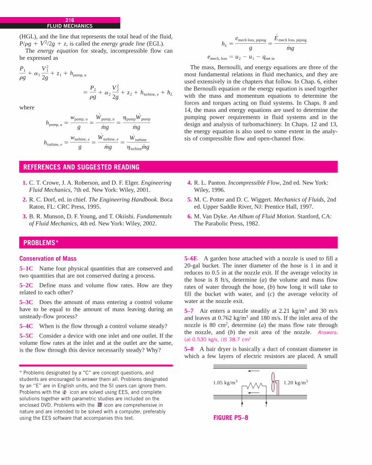
(HGL), and the line that represents the total head of the fluid,P/rg ' V2/2g ' z, is called the energy grade line (EGL).

The energy equation for steady, incompressible flow canbe expressed as

where

hturbine, e !wturbine, e

g!

W#

turbine, e

m#g

!W#

turbine

hturbinem#g

hpump, u !wpump, u

g!

W#

pump, u

m#g

!hpumpW

#pump

m#g

!P2

rg' a2

V 22

2g' z2 ' hturbine, e ' hL

P1

rg' a1

V 21

2g' z1 ' hpump, u

216FLUID MECHANICS

The mass, Bernoulli, and energy equations are three of themost fundamental relations in fluid mechanics, and they areused extensively in the chapters that follow. In Chap. 6, eitherthe Bernoulli equation or the energy equation is used togetherwith the mass and momentum equations to determine theforces and torques acting on fluid systems. In Chaps. 8 and14, the mass and energy equations are used to determine thepumping power requirements in fluid systems and in thedesign and analysis of turbomachinery. In Chaps. 12 and 13,the energy equation is also used to some extent in the analy-sis of compressible flow and open-channel flow.

emech, loss ! u2 " u1 " qnet in

hL !emech loss, piping

g!

E#

mech loss, piping

m#g

REFERENCES AND SUGGESTED READING

1. C. T. Crowe, J. A. Roberson, and D. F. Elger. EngineeringFluid Mechanics, 7th ed. New York: Wiley, 2001.

2. R. C. Dorf, ed. in chief. The Engineering Handbook. BocaRaton, FL: CRC Press, 1995.

3. B. R. Munson, D. F. Young, and T. Okiishi. Fundamentalsof Fluid Mechanics, 4th ed. New York: Wiley, 2002.

4. R. L. Panton. Incompressible Flow, 2nd ed. New York:Wiley, 1996.

5. M. C. Potter and D. C. Wiggert. Mechanics of Fluids, 2nded. Upper Saddle River, NJ: Prentice Hall, 1997.

6. M. Van Dyke. An Album of Fluid Motion. Stanford, CA:The Parabolic Press, 1982.

PROBLEMS*

Conservation of Mass5–1C Name four physical quantities that are conserved andtwo quantities that are not conserved during a process.

5–2C Define mass and volume flow rates. How are theyrelated to each other?

5–3C Does the amount of mass entering a control volumehave to be equal to the amount of mass leaving during anunsteady-flow process?

5–4C When is the flow through a control volume steady?

5–5C Consider a device with one inlet and one outlet. If thevolume flow rates at the inlet and at the outlet are the same,is the flow through this device necessarily steady? Why?

5–6E A garden hose attached with a nozzle is used to fill a20-gal bucket. The inner diameter of the hose is 1 in and itreduces to 0.5 in at the nozzle exit. If the average velocity inthe hose is 8 ft/s, determine (a) the volume and mass flowrates of water through the hose, (b) how long it will take tofill the bucket with water, and (c) the average velocity ofwater at the nozzle exit.

5–7 Air enters a nozzle steadily at 2.21 kg/m3 and 30 m/sand leaves at 0.762 kg/m3 and 180 m/s. If the inlet area of thenozzle is 80 cm2, determine (a) the mass flow rate throughthe nozzle, and (b) the exit area of the nozzle. Answers:(a) 0.530 kg/s, (b) 38.7 cm2

5–8 A hair dryer is basically a duct of constant diameter inwhich a few layers of electric resistors are placed. A small

1.05 kg/m3 1.20 kg/m3

FIGURE P5–8

* Problems designated by a “C” are concept questions, andstudents are encouraged to answer them all. Problems designatedby an “E” are in English units, and the SI users can ignore them.Problems with the icon are solved using EES, and completesolutions together with parametric studies are included on theenclosed DVD. Problems with the icon are comprehensive innature and are intended to be solved with a computer, preferablyusing the EES software that accompanies this text.

cen72367_ch05.qxd 10/29/04 2:25 PM Page 216

CHAPTER 5217

5–13 A smoking lounge is to accommodate 15 heavysmokers. The minimum fresh air requirement for smokinglounges is specified to be 30 L/s per person (ASHRAE, Stan-dard 62, 1989). Determine the minimum required flow rate offresh air that needs to be supplied to the lounge, and thediameter of the duct if the air velocity is not to exceed 8 m/s.

217CHAPTER 5

Bathroom22°C

Fan

30 L/s

FIGURE P5–11

Airoutlet

Exhaustfan

Airinlet

FIGURE P5–12

5–12 A desktop computer is to be cooled by a fan whoseflow rate is 0.34 m3/min. Determine the mass flow rate of airthrough the fan at an elevation of 3400 m where the air den-sity is 0.7 kg/m3. Also, if the average velocity of air is not toexceed 110 m/min, determine the diameter of the casing ofthe fan. Answers: 0.238 kg/min, 0.063 m

Smokinglounge

15 smokersFan

FIGURE P5–13

5–14 The minimum fresh air requirement of a residentialbuilding is specified to be 0.35 air change per hour(ASHRAE, Standard 62, 1989). That is, 35 percent of theentire air contained in a residence should be replaced byfresh outdoor air every hour. If the ventilation requirement ofa 2.7-m-high, 200-m2 residence is to be met entirely by a fan,determine the flow capacity in L/min of the fan that needs tobe installed. Also determine the diameter of the duct if the airvelocity is not to exceed 6 m/s.

fan pulls the air in and forces it through the resistors where itis heated. If the density of air is 1.20 kg/m3 at the inlet and1.05 kg/m3 at the exit, determine the percent increase in thevelocity of air as it flows through the dryer.

5–9E Air whose density is 0.078 lbm/ft3 enters the duct ofan air-conditioning system at a volume flow rate of 450ft3/min. If the diameter of the duct is 10 in, determine thevelocity of the air at the duct inlet and the mass flow rate ofair.

5–10 A 1-m3 rigid tank initially contains air whose densityis 1.18 kg/m3. The tank is connected to a high-pressure sup-ply line through a valve. The valve is opened, and air isallowed to enter the tank until the density in the tank rises to7.20 kg/m3. Determine the mass of air that has entered thetank. Answer: 6.02 kg

5–11 The ventilating fan of the bathroom of a building hasa volume flow rate of 30 L/s and runs continuously. If thedensity of air inside is 1.20 kg/m3, determine the mass of airvented out in one day.

cen72367_ch05.qxd 10/29/04 2:25 PM Page 217

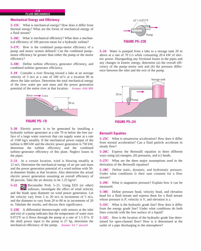
Mechanical Energy and Efficiency5–15C What is mechanical energy? How does it differ fromthermal energy? What are the forms of mechanical energy ofa fluid stream?

5–16C What is mechanical efficiency? What does a mechan-ical efficiency of 100 percent mean for a hydraulic turbine?

5–17C How is the combined pump–motor efficiency of apump and motor system defined? Can the combined pump–motor efficiency be greater than either the pump or the motorefficiency?

5–18C Define turbine efficiency, generator efficiency, andcombined turbine–generator efficiency.

5–19 Consider a river flowing toward a lake at an averagevelocity of 3 m/s at a rate of 500 m3/s at a location 90 mabove the lake surface. Determine the total mechanical energyof the river water per unit mass and the power generationpotential of the entire river at that location. Answer: 444 MW

218FLUID MECHANICS

5–24 Water is pumped from a lake to a storage tank 20 mabove at a rate of 70 L/s while consuming 20.4 kW of elec-tric power. Disregarding any frictional losses in the pipes andany changes in kinetic energy, determine (a) the overall effi-ciency of the pump–motor unit and (b) the pressure differ-ence between the inlet and the exit of the pump.

"T = 0.072°F

Pump

FIGURE P5–23E

5–20 Electric power is to be generated by installing ahydraulic turbine–generator at a site 70 m below the free sur-face of a large water reservoir that can supply water at a rateof 1500 kg/s steadily. If the mechanical power output of theturbine is 800 kW and the electric power generation is 750 kW,determine the turbine efficiency and the combinedturbine–generator efficiency of this plant. Neglect losses inthe pipes.

5–21 At a certain location, wind is blowing steadily at12 m/s. Determine the mechanical energy of air per unit massand the power generation potential of a wind turbine with 50-m-diameter blades at that location. Also determine the actualelectric power generation assuming an overall efficiency of30 percent. Take the air density to be 1.25 kg/m3.

5–22 Reconsider Prob. 5–21. Using EES (or other)software, investigate the effect of wind velocity

and the blade span diameter on wind power generation. Letthe velocity vary from 5 to 20 m/s in increments of 5 m/s,and the diameter to vary from 20 to 80 m in increments of 20m. Tabulate the results, and discuss their significance.

5–23E A differential thermocouple with sensors at the inletand exit of a pump indicates that the temperature of water rises0.072°F as it flows through the pump at a rate of 1.5 ft3/s. Ifthe shaft power input to the pump is 27 hp, determine themechanical efficiency of the pump. Answer: 64.7 percent

Pump

Storage tank

20 m

FIGURE P5–24

River 3 m/s

90 m

FIGURE P5–19

Bernoulli Equation5–25C What is streamwise acceleration? How does it differfrom normal acceleration? Can a fluid particle accelerate insteady flow?

5–26C Express the Bernoulli equation in three differentways using (a) energies, (b) pressures, and (c) heads.

5–27C What are the three major assumptions used in thederivation of the Bernoulli equation?

5–28C Define static, dynamic, and hydrostatic pressure.Under what conditions is their sum constant for a flowstream?

5–29C What is stagnation pressure? Explain how it can bemeasured.

5–30C Define pressure head, velocity head, and elevationhead for a fluid stream and express them for a fluid streamwhose pressure is P, velocity is V, and elevation is z.

5–31C What is the hydraulic grade line? How does it differfrom the energy grade line? Under what conditions do bothlines coincide with the free surface of a liquid?

5–32C How is the location of the hydraulic grade line deter-mined for open-channel flow? How is it determined at theoutlet of a pipe discharging to the atmosphere?

cen72367_ch05.qxd 10/29/04 2:25 PM Page 218

CHAPTER 5219

5–33C The water level of a tank on a building roof is 20 mabove the ground. A hose leads from the tank bottom to theground. The end of the hose has a nozzle, which is pointedstraight up. What is the maximum height to which the watercould rise? What factors would reduce this height?

5–34C In a certain application, a siphon must go over ahigh wall. Can water or oil with a specific gravity of 0.8 goover a higher wall? Why?

5–35C Explain how and why a siphon works. Someoneproposes siphoning cold water over a 7-m-high wall. Is thisfeasible? Explain.

5–36C A student siphons water over a 8.5-m-high wall atsea level. She then climbs to the summit of Mount Shasta(elevation 4390 m, Patm ! 58.5 kPa) and attempts the sameexperiment. Comment on her prospects for success.

5–37C A glass manometer with oil as the working fluid isconnected to an air duct as shown in Fig. P5–37C. Will theoil in the manometer move as in Fig. P5–37Ca or b? Explain.What would your response be if the flow direction isreversed?

shoots up to 34 m. Estimate the gage pressure of water in thepipe. State your assumptions and discuss if the actual pres-sure is more or less than the value you predicted.

5–40 A Pitot-static probe is used to measure the velocity ofan aircraft flying at 3000 m. If the differential pressure read-ing is 3 kPa, determine the velocity of the aircraft.

5–41 While traveling on a dirt road, the bottom of a car hitsa sharp rock and a small hole develops at the bottom of itsgas tank. If the height of the gasoline in the tank is 30 cm,determine the initial velocity of the gasoline at the hole. Dis-cuss how the velocity will change with time and how theflow will be affected if the lid of the tank is closed tightly.Answer: 2.43 m/s

5–42E The drinking water needs of an office are metby large water bottles. One end of a 0.25-in-

diameter plastic hose is inserted into the bottle placed on ahigh stand, while the other end with an on/off valve is main-tained 2 ft below the bottom of the bottle. If the water levelin the bottle is 1.5 ft when it is full, determine how long itwill take at the minimum to fill an 8-oz glass (! 0.00835 ft3)(a) when the bottle is first opened and (b) when the bottle isalmost empty.

219CHAPTER 5

Flow Flow

(a) (b)

FIGURE P5–37C

Flow

12

FIGURE P5–38C

5–38C The velocity of a fluid flowing in a pipe is to bemeasured by two different Pitot-type mercury manometersshown in Fig. P5–38C. Would you expect both manometersto predict the same velocity for flowing water? If not, whichwould be more accurate? Explain. What would your responsebe if air were flowing in the pipe instead of water?

Water1.5 ft

2 ft

FIGURE P5–42E

5–39 In cold climates, water pipes may freeze and burst ifproper precautions are not taken. In such an occurrence, theexposed part of a pipe on the ground ruptures, and water

5–43 A piezometer and a Pitot tube are tapped into a 3-cm-diameter horizontal water pipe, and the height of the watercolumns are measured to be 20 cm in the piezometer and 35cm in the Pitot tube (both measured from the top surface ofthe pipe). Determine the velocity at the center of the pipe.

5–44 The diameter of a cylindrical water tank is Do and itsheight is H. The tank is filled with water, which is open tothe atmosphere. An orifice of diameter Do with a smoothentrance (i.e., no losses) is open at the bottom. Develop arelation for the time required for the tank (a) to emptyhalfway and (b) to empty completely.

cen72367_ch05.qxd 10/29/04 2:25 PM Page 219

5–45 A pressurized tank of water has a 10-cm-diameter ori-fice at the bottom, where water discharges to the atmosphere.The water level is 3 m above the outlet. The tank air pressureabove the water level is 300 kPa (absolute) while the atmos-pheric pressure is 100 kPa. Neglecting frictional effects,determine the initial discharge rate of water from the tank.Answer: 0.168 m3/s

220FLUID MECHANICS

the frictional losses are negligible. If the tank is initiallyempty, (a) determine the maximum height that the water willreach in the tank and (b) obtain a relation for water height zas a function of time.

5–49E Water flows through a horizontal pipe at a rate of 1gal/s. The pipe consists of two sections of diameters 4 in and2 in with a smooth reducing section. The pressure differencebetween the two pipe sections is measured by a mercurymanometer. Neglecting frictional effects, determine the dif-ferential height of mercury between the two pipe sections.Answer: 0.52 in

Doz

DT

m*

FIGURE P5–48

5–46 Reconsider Prob. 5–45. Using EES (or other)software, investigate the effect of water height in

the tank on the discharge velocity. Let the water height varyfrom 0 to 5 m in increments of 0.5 m. Tabulate and plot theresults.

5–47E A siphon pumps water from a large reservoir to alower tank that is initially empty. The tank also has a roundedorifice 15 ft below the reservoir surface where the waterleaves the tank. Both the siphon and the orifice diameters are2 in. Ignoring frictional losses, determine to what height thewater will rise in the tank at equilibrium.

5–48 Water enters a tank of diameter DT steadily at a massflow rate of m

.in. An orifice at the bottom with diameter Do

allows water to escape. The orifice has a rounded entrance, so

4 in 2 in

h

FIGURE P5–49E

3 m

10 cm

Air300 kPa

FIGURE P5–45

5–50 An airplane is flying at an altitude of 12,000 m.Determine the gage pressure at the stagnation point on thenose of the plane if the speed of the plane is 200 km/h. Howwould you solve this problem if the speed were 1050 km/h?Explain.

5–51 The air velocity in the duct of a heating system is tobe measured by a Pitot-static probe inserted into the duct par-allel to flow. If the differential height between the watercolumns connected to the two outlets of the probe is 2.4 cm,determine (a) the flow velocity and (b) the pressure rise atthe tip of the probe. The air temperature and pressure in theduct are 45°C and 98 kPa, respectively.

5–52 The water in a 10-m-diameter, 2-m-high abovegroundswimming pool is to be emptied by unplugging a 3-cm-diameter, 25-m-long horizontal pipe attached to the bottom ofthe pool. Determine the maximum discharge rate of waterthrough the pipe. Also, explain why the actual flow rate willbe less.

5–53 Reconsider Prob. 5–52. Determine how long it willtake to empty the swimming pool completely. Answer: 19.7 h

5–54 Reconsider Prob. 5–53. Using EES (or other)software, investigate the effect of the discharge

pipe diameter on the time required to empty the pool com-pletely. Let the diameter vary from 1 to 10 cm in incrementsof 1 cm. Tabulate and plot the results.

5–55 Air at 110 kPa and 50°C flows upward through a 6-cm-diameter inclined duct at a rate of 45 L/s. The ductdiameter is then reduced to 4 cm through a reducer. Thepressure change across the reducer is measured by a water

cen72367_ch05.qxd 10/29/04 2:25 PM Page 220

CHAPTER 5221

manometer. The elevation difference between the two pointson the pipe where the two arms of the manometer areattached is 0.20 m. Determine the differential height betweenthe fluid levels of the two arms of the manometer.

5–60 A Pitot-static probe connected to a water manometeris used to measure the velocity of air. If the deflection (thevertical distance between the fluid levels in the two arms) is7.3 cm, determine the air velocity. Take the density of air tobe 1.25 kg/m3.

221CHAPTER 5

Air

h

FIGURE P5–55

2.6 in

12.2 psia

Air 1.8 in

11.8 psia

FIGURE P5–56E

5–56E Air is flowing through a venturi meter whose diame-ter is 2.6 in at the entrance part (location 1) and 1.8 in at thethroat (location 2). The gage pressure is measured to be 12.2psia at the entrance and 11.8 psia at the throat. Neglectingfrictional effects, show that the volume flow rate can beexpressed as

and determine the flow rate of air. Take the air density to be0.075 lbm/ft3.

V#

! A2B 2(P1 " P2)

r(1 " A22/A

21)

5 cm Air

0.3 cm

10 cm

20 cm

Liquidrising

FIGURE P5–58

5–57 The water pressure in the mains of a city at a particu-lar location is 400 kPa gage. Determine if this main can servewater to neighborhoods that are 50 m above this location.

5–58 A handheld bicycle pump can be used as an atomizerto generate a fine mist of paint or pesticide by forcing air at ahigh velocity through a small hole and placing a short tubebetween the liquid reservoir and the high-speed air jet whoselow pressure drives the liquid up through the tube. In such anatomizer, the hole diameter is 0.3 cm, the vertical distancebetween the liquid level in the tube and the hole is 10 cm,and the bore (diameter) and the stroke of the air pump are 5cm and 20 cm, respectively. If the atmospheric conditions are20°C and 95 kPa, determine the minimum speed that the pis-ton must be moved in the cylinder during pumping to initiatethe atomizing effect. The liquid reservoir is open to the atmo-sphere.

Pitot-staticprobe

Manometer

Air 7.3 cm

FIGURE P5–60

20 m

2 atm

h

FIGURE P5–59

5–59 The water level in a tank is 20 m above the ground. Ahose is connected to the bottom of the tank, and the nozzle atthe end of the hose is pointed straight up. The tank cover isairtight, and the air pressure above the water surface is 2 atmgage. The system is at sea level. Determine the maximumheight to which the water stream could rise. Answer: 40.7 m

5–61E The air velocity in a duct is measured by a Pitot-staticprobe connected to a differential pressure gage. If the air is at13.4 psia absolute and 70°F and the reading of the differen-tial pressure gage is 0.15 psi, determine the air velocity.Answer: 143 ft/s

cen72367_ch05.qxd 10/29/04 2:25 PM Page 221

5–62 In a hydroelectric power plant, water enters the tur-bine nozzles at 700 kPa absolute with a low velocity. If thenozzle outlets are exposed to atmospheric pressure of 100 kPa,determine the maximum velocity to which water can beaccelerated by the nozzles before striking the turbine blades.

Energy Equation5–63C Consider the steady adiabatic flow of an incom-pressible fluid. Can the temperature of the fluid decrease dur-ing flow? Explain.

5–64C Consider the steady adiabatic flow of an incom-pressible fluid. If the temperature of the fluid remains con-stant during flow, is it accurate to say that the frictionaleffects are negligible?

5–65C What is irreversible head loss? How is it related tothe mechanical energy loss?

5–66C What is useful pump head? How is it related to thepower input to the pump?

5–67C What is the kinetic energy correction factor? Is itsignificant?

5–68C The water level in a tank is 20 m above the ground.A hose is connected to the bottom of the tank, and the nozzleat the end of the hose is pointed straight up. The water streamfrom the nozzle is observed to rise 25 m above the ground.Explain what may cause the water from the hose to riseabove the tank level.

5–69 Underground water is to be pumped by a 70 percentefficient 3-kW submerged pump to a pool whose free surfaceis 30 m above the underground water level. The diameter ofthe pipe is 7 cm on the intake side and 5 cm on the dischargeside. Determine (a) the maximum flow rate of water and(b) the pressure difference across the pump. Assume the eleva-tion difference between the pump inlet and the outlet and theeffect of the kinetic energy correction factors to be negligible.

222FLUID MECHANICS

5–74 Water is being pumped from a large lake to a reser-voir 25 m above at a rate of 25 L/s by a 10-kW (shaft) pump.If the irreversible head loss of the piping system is 7 m,determine the mechanical efficiency of the pump. Answer:78.5 percent

5–75 Reconsider Prob. 5–74. Using EES (or other)software, investigate the effect of irreversible

head loss on the mechanical efficiency of the pump. Let thehead loss vary from 0 to 15 m in increments of 1 m. Plot theresults, and discuss them.

5–76 A 7-hp (shaft) pump is used to raise water to a 15-mhigher elevation. If the mechanical efficiency of the pump is82 percent, determine the maximum volume flow rate ofwater.

5–77 Water flows at a rate of 0.035 m3/s in a horizontal pipewhose diameter is reduced from 15 cm to 8 cm by a reducer.If the pressure at the centerline is measured to be 470 kPaand 440 kPa before and after the reducer, respectively, deter-mine the irreversible head loss in the reducer. Take thekinetic energy correction factors to be 1.05. Answer: 0.68 m

5–78 The water level in a tank is 20 m above the ground. Ahose is connected to the bottom of the tank, and the nozzle atthe end of the hose is pointed straight up. The tank is at sea

30 m

Pool

FIGURE P5–69

Air

8 m/s

Exhaustfan

FIGURE P5–73

5–71E In a hydroelectric power plant, water flows from anelevation of 240 ft to a turbine, where electric power is gen-erated. For an overall turbine–generator efficiency of 83 per-cent, determine the minimum flow rate required to generate100 kW of electricity. Answer: 370 lbm/s

5–72E Reconsider Prob. 5–71E. Determine the flow rate ofwater if the irreversible head loss of the piping system betweenthe free surfaces of the source and the sink is 36 ft.

5–73 A fan is to be selected to ventilate a bathroomwhose dimensions are 2 m # 3 m # 3 m. The

air velocity is not to exceed 8 m/s to minimize vibration andnoise. The combined efficiency of the fan–motor unit to beused can be taken to be 50 percent. If the fan is to replace theentire volume of air in 10 min, determine (a) the wattage ofthe fan–motor unit to be purchased, (b) the diameter of thefan casing, and (c) the pressure difference across the fan.Take the air density to be 1.25 kg/m3 and disregard the effectof the kinetic energy correction factors.

5–70 Reconsider Prob. 5–69. Determine the flow rate ofwater and the pressure difference across the pump if the irre-versible head loss of the piping system is 5 m.

cen72367_ch05.qxd 10/29/04 2:25 PM Page 222

CHAPTER 5223

level, and the water surface is open to the atmosphere. In theline leading from the tank to the nozzle is a pump, whichincreases the pressure of water. If the water jet rises to aheight of 27 m from the ground, determine the minimumpressure rise supplied by the pump to the water line.

lake to the reservoir at night using cheap power, and lettingthe water flow from the reservoir back to the lake during theday, producing power as the pump–motor operates as a tur-bine–generator during reverse flow. Preliminary analysisshows that a water flow rate of 2 m3/s can be used in eitherdirection, and the irreversible head loss of the piping systemis 4 m. The combined pump–motor and turbine–generatorefficiencies are expected to be 75 percent each. Assuming thesystem operates for 10 h each in the pump and turbine modesduring a typical day, determine the potential revenue thispump–turbine system can generate per year.

5–81 Water flows at a rate of 20 L/s through a horizontalpipe whose diameter is constant at 3 cm. The pressure dropacross a valve in the pipe is measured to be 2 kPa. Determinethe irreversible head loss of the valve, and the useful pump-ing power needed to overcome the resulting pressure drop.Answers: 0.204 m, 40 W

223CHAPTER 5

20 m

27 m

FIGURE P5–78

Pump–turbine

Lake

40 m

Reservoir

FIGURE P5–80

Water20 L/s

"P = 2 kPa

FIGURE P5–81

5–82E The water level in a tank is 66 ft above the ground.A hose is connected to the bottom of the tank at the groundlevel and the nozzle at the end of the hose is pointed straightup. The tank cover is airtight, but the pressure over the watersurface is unknown. Determine the minimum tank air pres-sure (gage) that will cause a water stream from the nozzle torise 90 ft from the ground.

5–83 A large tank is initially filled with water 2 m abovethe center of a sharp-edged 10-cm-diameter orifice. The tankwater surface is open to the atmosphere, and the orificedrains to the atmosphere. If the total irreversible head loss inthe system is 0.3 m, determine the initial discharge velocityof water from the tank. Take the kinetic energy correctionfactor at the orifice to be 1.2.

5–84 Water enters a hydraulic turbine through a 30-cm-diameter pipe at a rate of 0.6 m3/s and exits through a 25-cm-diameter pipe. The pressure drop in the turbine is measuredby a mercury manometer to be 1.2 m. For a combined turbine–generator efficiency of 83 percent, determine the net electric

5–79 A hydraulic turbine has 85 m of head available at aflow rate of 0.25 m3/s, and its overall turbine–generator effi-ciency is 78 percent. Determine the electric power output ofthis turbine.

5–80 The demand for electric power is usually much higherduring the day than it is at night, and utility companies oftensell power at night at much lower prices to encourage con-sumers to use the available power generation capacity and toavoid building new expensive power plants that will be usedonly a short time during peak periods. Utilities are also will-ing to purchase power produced during the day from privateparties at a high price.

Suppose a utility company is selling electric power for$0.03/kWh at night and is willing to pay $0.08/kWh forpower produced during the day. To take advantage of thisopportunity, an entrepreneur is considering building a largereservoir 40 m above the lake level, pumping water from the

cen72367_ch05.qxd 10/29/04 2:25 PM Page 223

power output. Disregard the effect of the kinetic energy cor-rection factors.

224FLUID MECHANICS

percent, determine the required shaft power input to the pumpand the water discharge velocity. Answers: 200 kW, 50.9 m/s

35 kW

"P = 400 kPa

0.1 m3/s

Motor

8 cm

12 cm

Oil

Pump

FIGURE P5–86

5–85 The velocity profile for turbulent flow in a circularpipe is usually approximated as u(r) ! umax(1 " r/R)1/n,where n ! 7. Determine the kinetic energy correction factorfor this flow. Answer: 1.06

5–86 An oil pump is drawing 35 kW of electric powerwhile pumping oil with r ! 860 kg/m3 at a rate of 0.1 m3/s.The inlet and outlet diameters of the pipe are 8 cm and 12 cm,respectively. If the pressure rise of oil in the pump is mea-sured to be 400 kPa and the motor efficiency is 90 percent,determine the mechanical efficiency of the pump. Take thekinetic energy correction factor to be 1.05.

4 m

FIGURE P5–88

5–87E A 73-percent efficient 12-hp pump is pumping waterfrom a lake to a nearby pool at a rate of 1.2 ft3/s through aconstant-diameter pipe. The free surface of the pool is 35 ftabove that of the lake. Determine the irreversible head loss ofthe piping system, in ft, and the mechanical power used toovercome it.

5–88 A fireboat is to fight fires at coastal areas by drawingseawater with a density of 1030 kg/m3 through a 20-cm-diam-eter pipe at a rate of 0.1 m3/s and discharging it through ahose nozzle with an exit diameter of 5 cm. The total irre-versible head loss of the system is 3 m, and the position of thenozzle is 4 m above sea level. For a pump efficiency of 70

We*

30 cm Turbine

"P = 1.2 m Hg

Generator

25 cm

FIGURE P5–84 Review Problems5–89 A D0 ! 10-m-diameter tank is initially filled withwater 2 m above the center of a D ! 10-cm-diameter valvenear the bottom. The tank surface is open to the atmosphere,and the tank drains through a L ! 100-m-long pipe con-nected to the valve. The friction factor of the pipe is given tobe f ! 0.015, and the discharge velocity is expressed as

where z is the water height above the center

of the valve. Determine (a) the initial discharge velocity fromthe tank and (b) the time required to empty the tank. The tankcan be considered to be empty when the water level drops tothe center of the valve.

5–90 Underground water is being pumped into a poolwhose cross section is 3 m # 4 m while water is dischargedthrough a 5-cm-diameter orifice at a constant average veloc-ity of 5 m/s. If the water level in the pool rises at a rate of 1.5cm/min, determine the rate at which water is supplied to thepool, in m3/s.

5–91 The velocity of a liquid flowing in a circular pipe ofradius R varies from zero at the wall to a maximum at thepipe center. The velocity distribution in the pipe can be repre-sented as V(r), where r is the radial distance from the pipecenter. Based on the definition of mass flow rate m

., obtain a

relation for the average velocity in terms of V(r), R, and r.

5–92 Air at 4.18 kg/m3 enters a nozzle that has an inlet-to-exit area ratio of 2:1 with a velocity of 120 m/s and leaveswith a velocity of 380 m/s. Determine the density of air at theexit. Answer: 2.64 kg/m3

5–93 The air in a 6-m # 5-m # 4-m hospital room is to becompletely replaced by conditioned air every 20 min. If theaverage air velocity in the circular air duct leading to theroom is not to exceed 5 m/s, determine the minimum diame-ter of the duct.

5–94 A pressurized 2-m-diameter tank of water has a 10-cm-diameter orifice at the bottom, where water discharges tothe atmosphere. The water level initially is 3 m above the

V !B 2gz

1.5 ' fL/D

cen72367_ch05.qxd 10/29/04 2:25 PM Page 224

CHAPTER 5225

outlet. The tank air pressure above the water level is main-tained at 450 kPa absolute and the atmospheric pressure is100 kPa. Neglecting frictional effects, determine (a) howlong it will take for half of the water in the tank to be dis-charged and (b) the water level in the tank after 10 s.

5–95 Air flows through a pipe at a rate of 200 L/s. The pipeconsists of two sections of diameters 20 cm and 10 cm with asmooth reducing section that connects them. The pressuredifference between the two pipe sections is measured by awater manometer. Neglecting frictional effects, determine thedifferential height of water between the two pipe sections.Take the air density to be 1.20 kg/m3. Answer: 3.7 cm

5–98 Water is flowing through a Venturi meter whose diam-eter is 7 cm at the entrance part and 4 cm at the throat. Thepressure is measured to be 430 kPa at the entrance and 120kPa at the throat. Neglecting frictional effects, determine theflow rate of water. Answer: 0.538 m3/s

5–99E The water level in a tank is 80 ft above the ground.A hose is connected to the bottom of the tank, and the nozzleat the end of the hose is pointed straight up. The tank is atsea level, and the water surface is open to the atmosphere. Inthe line leading from the tank to the nozzle is a pump, whichincreases the water pressure by 10 psia. Determine the maxi-mum height to which the water stream could rise.

5–100 A wind tunnel draws atmospheric air at 20°C and101.3 kPa by a large fan located near the exit of the tunnel. Ifthe air velocity in the tunnel is 80 m/s, determine the pressurein the tunnel.

20 cmAir200 L/s

10 cm

h

FIGURE P5–95

2 cmAir102 kPa

100 kPa20°C

2 cm

4 cm

FIGURE P5–97

5–96 Air at 100 kPa and 25°C flows in a horizontalduct of variable cross section. The water column

in the manometer that measures the difference between twosections has a vertical displacement of 8 cm. If the velocityin the first section is low and the friction is negligible, deter-mine the velocity at the second section. Also, if the manome-ter reading has a possible error of -2 mm, conduct an erroranalysis to estimate the range of validity for the velocityfound.

5–97 A very large tank contains air at 102 kPa at a locationwhere the atmospheric air is at 100 kPa and 20°C. Now a 2-cm-diameter tap is opened. Determine the maximum flow rateof air through the hole. What would your response be if air isdischarged through a 2-m-long, 4-cm-diameter tube with a 2-cm-diameter nozzle? Would you solve the problem the sameway if the pressure in the storage tank were 300 kPa?

20°C101.3 kPa

Wind tunnel

80 m/s

FIGURE P5–100

2 mWater

10 cm100 m

FIGURE P5–102

5–101 Water flows at a rate of 0.025 m3/s in a horizontalpipe whose diameter increases from 6 to 11 cm by anenlargement section. If the head loss across the enlargementsection is 0.45 m and the kinetic energy correction factor atboth the inlet and the outlet is 1.05, determine the pressurechange.

5–102 A 2-m-high large tank is initially filled with water.The tank water surface is open to the atmosphere, and asharp-edged 10-cm-diameter orifice at the bottom drains tothe atmosphere through a horizontal 100-m-long pipe. If thetotal irreversible head loss of the system is determined to be1.5 m, determine the initial velocity of the water from thetank. Disregard the effect of the kinetic energy correction fac-tors. Answer: 3.13 m/s

cen72367_ch05.qxd 10/29/04 2:25 PM Page 225

5–103 Reconsider Prob. 5–102. Using EES (or other)software, investigate the effect of the tank

height on the initial discharge velocity of water from thecompletely filled tank. Let the tank height vary from 2 to 15m in increments of 1 m, and assume the irreversible head lossto remain constant. Tabulate and plot the results.

5–104 Reconsider Prob. 5–102. In order to drain the tankfaster, a pump is installed near the tank exit. Determine thepump head input necessary to establish an average watervelocity of 6 m/s when the tank is full.

Design and Essay Problems5–105 Using a large bucket whose volume is known andmeasuring the time it takes to fill the bucket with water froma garden hose, determine the mass flow rate and the averagevelocity of water through the hose.

5–106 Your company is setting up an experiment thatinvolves the measurement of airflow rate in a duct, and youare to come up with proper instrumentation. Research theavailable techniques and devices for airflow rate measure-ment, discuss the advantages and disadvantages of each tech-nique, and make a recommendation.

5–107 Computer-aided designs, the use of better materials,and better manufacturing techniques have resulted in atremendous increase in the efficiency of pumps, turbines, andelectric motors. Contact several pump, turbine, and motormanufacturers and obtain information about the efficiency oftheir products. In general, how does efficiency vary withrated power of these devices?

226FLUID MECHANICS

5–108 Using a handheld bicycle pump to generate an airjet, a soda can as the water reservoir, and a straw as the tube,design and build an atomizer. Study the effects of variousparameters such as the tube length, the diameter of the exithole, and the pumping speed on performance.

5–109 Using a flexible drinking straw and a ruler, explainhow you would measure the water flow velocity in a river.

5–110 The power generated by a wind turbine is propor-tional to the cube of the wind velocity. Inspired by the accel-eration of a fluid in a nozzle, someone proposes to install areducer casing to capture the wind energy from a larger areaand accelerate it before the wind strikes the turbine blades, asshown in Fig. P5–110. Evaluate if the proposed modificationshould be given a consideration in the design of new windturbines.

Wind

FIGURE P5–110

cen72367_ch05.qxd 10/29/04 2:25 PM Page 226