Can Pro-Marriage Policies Work? An Analysis of Marginal Marriages

by

Wolfgang FRIMMEL Martin HALLA

Rudolf WINTER-EBMER

Working Paper No. 1209 July 2012

DEPARTMENT OF ECONOMICSJOHANNES KEPLER UNIVERSITY OF

LINZ

Johannes Kepler University of Linz Department of Economics

Altenberger Strasse 69 A-4040 Linz - Auhof, Austria

www.econ.jku.at

Rudolf.Winterebmer@jku.at phone +43 (0)70 2468 -8236, -8238 (fax)

Can Pro-Marriage Policies Work?

An Analysis of Marginal Marriages

⇤

Wolfgang Frimmel Martin Halla Rudolf Winter-EbmerUniversity of Linz University of Linz & IZA University of Linz, IHS,

IZA & CEPR

October 3, 2013(First version: July 2012)

Abstract

Policies to promote marriage are controversial, and it is unclear whether theyare successful. To analyze such policies, it is essential to distinguish between amarriage that is created by a marriage-promoting policy (marginal marriage) anda marriage that would have been formed even in the absence of a state interven-tion (average marriage). In this paper, we exploit the suspension of a cash-on-handmarriage subsidy in Austria to examine the differential behavior of marginal and av-erage marriages. The announcement of this suspension led to an enormous marriageboom (plus 350 percent) among eligible couples that allows us to locate marginalmarriages. Applying a difference-in-differences approach, we show that marginalmarriages are surprisingly as stable as average marriages. However, they have fewerchildren, have them later in marriage, and their children are less healthy at birth.

JEL Classification: J12, H24, H53, I38.Keywords: Marriage-promoting policies, marriage subsidies, marital instability, di-vorce, fertility, health at birth.

⇤For helpful discussion and comments we would like to thank Raj Chetty, Jungmin Lee, DanielS. Hamermesh, Shelly Lundberg, Enrico Moretti, Helmut Rainer, Mario Schnalzenberger, BetseyStevenson, Andrea Weber, Josef Zweimüller and participants at several seminars (Austrian NationalBank, Strathclyde, National Taiwan University, Vienna University of Economics and Business, ETHZurich, St. Gallen, Berlin Network of Labor Market Researchers, and Cesifo Munich) and conferences(ESPE in Essen, ASSA in Denver, AEA in Graz, EEA in Oslo, and VfS in Frankfurt). We arealso grateful for very helpful comments provided by the Editor and two anonymous referees. Theusual disclaimer applies. This research was funded by the Austrian Science Fund (FWF): NationalResearch Network S103, The Austrian Center for Labor Economics and the Analysis of the Wel-fare State. A previous version of this paper was circulated 2010 under the title ‘Marriage Subsi-dies and Divorce: An Analysis of Marginal Marriages’. A Web Appenidx provides addition material:http://www.econ.jku.at/papers/2012/wp1209_web-appendix.pdf.

1 Introduction

Policies to promote marriage are controversial (McLanahan, 2007; Amato, 2007a,b; Fursten-

berg, 2007a,b; Struening, 2007). While there is extensive empirical literature (Waite and

Gallagher, 2000) documenting a strong correlation between being married and better

family outcomes, scholars do not agree whether this is a causal relationship. A host of

confounding factors that further marriage may also be beneficial to the outcomes under

consideration, and the debate seems far from settled.

This statistical debate is accompanied by a political debate, which reflects a basic

disagreement about whether the state should intervene in the private sphere. Liberal

activists believe that unmarried relationships deserve the same acceptance and support

as marriage. The feminist movement argues that existing policies to encourage mar-

riage reinforce traditional gender roles, and homosexual rights groups object that they

are indefensible since they exclude same-sex couples. On the other side, the marriage

movement— a loose group of conservatives and religious leaders — favors public policies

that strengthen the institution of marriage (Cherlin, 2003).

In this paper, we solve neither the statistical nor the political debate, but we do add

yet another important (and so far neglected) aspect to this controversy. Supporters of

marriage promotion contend that couples (and especially their children) should be better

off within a marriage.1 However, even under the assumption that marriage on average

causally improves family outcomes, it is a priori unclear whether the state should pursue

a pro-marriage agenda. The right question to ask is whether marriage improves the well-

being of the couples who marry because of a marriage-promoting policy.

For our argument, it is essential to distinguish between an average marriage and a

marginal marriage. We use the term average marriage to describe a couple who would

marry with or without a state intervention. In contrast, a marginal marriage is given by

spouses who would not have married without the state intervention.2

1In theory, legal marriage may increase well-being (as compared to cohabitation) if marriage acts as acommitment device that fosters co-operation and/or induces partners to make more relationship-specificinvestments (Matouschek and Rasul, 2008); this argument presumes that it is more costly to exit amarriage as compared to ending cohabitation.

2Conceptually we relate here to the treatment effect literature and employ a framework of potential

2

In order to account for the possibility that a policy affects the timing of marriage, we

introduce a third type of marriage: early average marriage. An early average marriage is

defined by spouses who would have married in the counterfactual situation (i.e. in absence

of the policy suspension), but not on the same date; they would have married later. That

means, in total we distinguish between three different types of marriages; depending on

their behavior in the absence of the policy suspension:

• Average marriage: spouses who would have married on the same date

• Early average marriage: spouses who would have married, but later

• Marginal marriage: spouses who would not have married in the absence of the policy

The distinction between the first and the second type introduces a conceptual consid-

eration of the difference between selection and timing. We assume that early average

marriages and average marriages are not substantially different with respect to other

dimensions apart from timing.

It is possible that marriage improves the well-being of average marriages but is not

(as) beneficial to marginal couples. Loosely speaking, it is important to know how dif-

ferent these two types of marriages are. Given that the benefits of marriage require a

certain level of marital stability to materialize, the most important question is whether

marginal marriages are as stable as average marriages. Moreover, expected or actual sta-

bility is a prerequisite for marital investment. If children are the targeted beneficiaries

of pro-marriage policies, a successful state intervention also requires that stable marginal

marriages will have offspring. We think of these conditions as necessary (but not sufficient)

conditions for marriage-promoting policies to work.

Based on theoretical grounds (Becker, 1973, 1974), however, we expect marginal mar-

riages to have a lower match quality (as compared to average marriages), to be less willing

to make marriage-specific investments such as children, and to exhibit a comparably higher

baseline divorce risk. If these gradients predicted by theory turn out to be empirically

relevant, a marriage-promoting policy is bound to fail because marginal marriages may be

outcomes (also called counterfactual reasoning). In the terminology of this literature, one could termmarginal marriages compliers and average marriages always-takers (Imbens and Angrist, 1994).

3

short-lived and may not produce children.3 Thus understanding how selective marginal

marriages are in terms of marital stability and fertility behavior is of particular interest

to researchers and policy-makers alike. Answering this question is empirically challeng-

ing, since an individual classification of average, early average, and marginal marriage is

impossible. We use a research design where a fair approximation of the shares of these

three groups is sufficient to estimate the selection effect.

In particular, we use the suspension of a straightforward cash-on-hand marriage-

promoting policy in Austria. Since the early seventies, two Austrian citizens, both mar-

rying for the first time, received approximately EUR 4, 250 or USD 5, 680 (values are

adjusted for inflation; 2010). At the end of August 1987, the suspension of this marriage

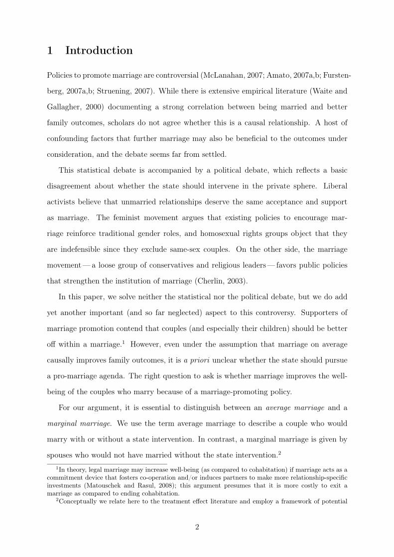
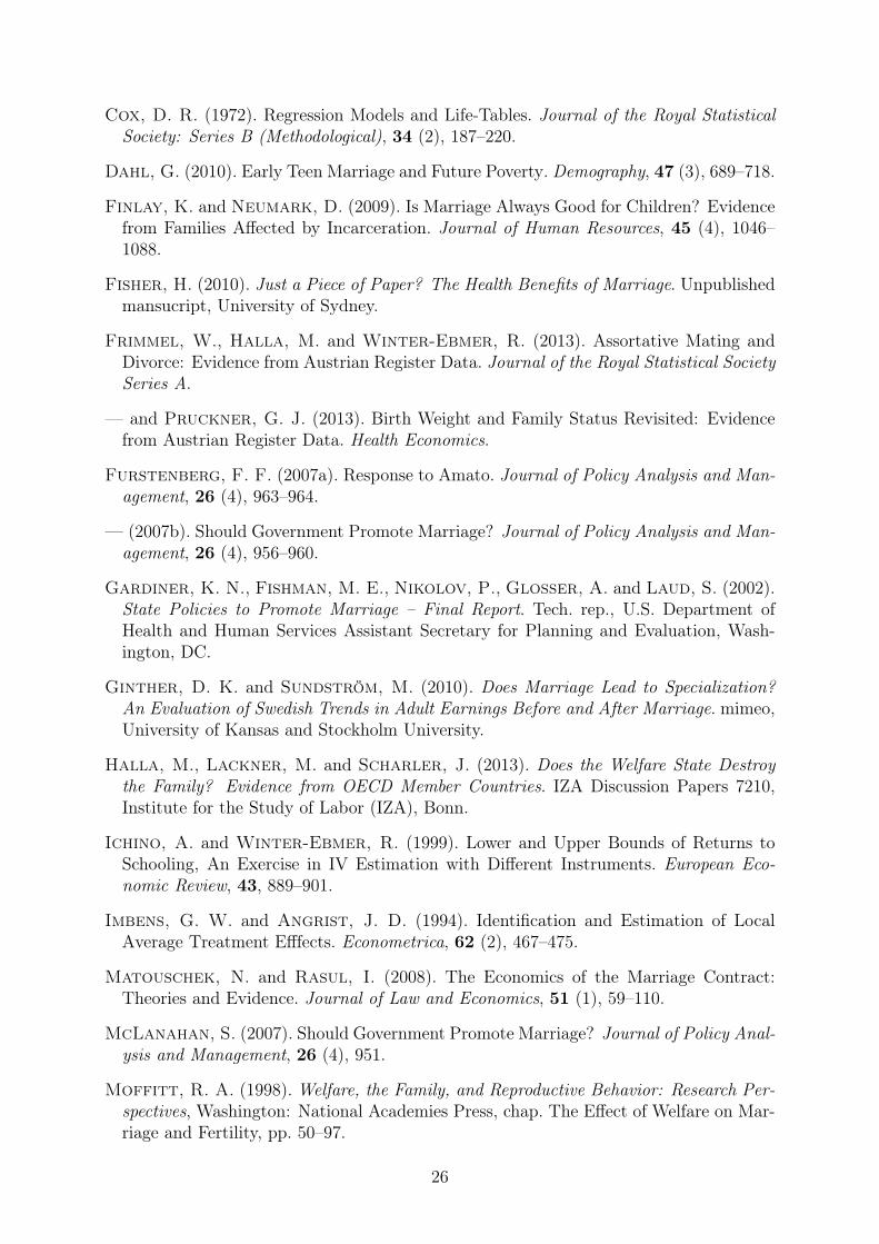
subsidy was announced to be effective as of January 1, 1988. This led to an enormous

marriage boom of more than 350 percent (see Figure 1). Clearly, part of the marriage

boom was simply due to timing (i.e. early average marriages). However, using individual-

level data on the entirety of Austrian marriages, we show that approximately half of the

couples who married between October and December 1987 were motivated by the cash

transfer and thus constitute marginal marriages.

[ Insert Figure 1 around here ]

For our estimation analysis, we exploit the eligibility criteria to set up a difference-

in-differences framework. This allows us to estimate the differential divorce and fertility

behavior of marginal couples. Quite surprisingly, we find hardly any evidence of a lower

marital stability of marginal marriages. We do find, however, that marginal marriages

have fewer children and have them later in marriage. The children born to marginal

marriages exhibit a lower health at birth.

Our findings contribute to different strands of economic literature and hold important

implications for public policy-makers. First, there is a strand of literature that asks the

fundamental question of whether the state can effectively encourage people to marry or

to stay married. While empirical work consistently shows that individuals respond to3In a worst case scenario, the state may create unstable marriages with additional children, that is,

children who would have not been conceived in the counterfactual state without policy intervention.

4

tax incentives in their marital decisions, as predicted by theory, the magnitudes of these

effects are typically small or short-lived (e. g., Whittington and Alm, 1997; Alm, Dickert-

Conlin and Whittington, 1999). The empirical evidence on behavioral effects created

by transfer programs is less consistent. However, Moffitt (1998) concludes based on a

comprehensive survey of the literature from the last three decades that transfer programs

do affect marital decisions as well. As argued by Blank (2002), it is typically difficult to

identify effects of tax and welfare reforms on family formation. These reforms are often

complicated, only a relatively small share of the population gets married in any given

year, and family behavior seems to be much more sluggish and resistant as compared to

labor market behavior. In contrast, the reform studied in our paper was straightforward

and had an obvious and enormous effect on marriage behavior.

Second, our paper relates to the literature interested in the effects of marriage. Only

a small number of studies offer a credible research design to identify a causal effect of

marriage. Almost all of these papers exploit exogenous variation in marital status due to

some kind of policy intervention. Two papers use a marriage boom in Sweden — created by

the Swedish widow’s pension reform in 1989—to estimate the corresponding treatment

effect of marriage on children’s school outcomes (Björklund, Ginther and Sundström,

2007) and on spouses’ labor market outcomes (Ginther and Sundström, 2010). The first

paper does not find any effect of marriage on children’s school performance. The second

finds a small marriage premium for men and a small marriage penalty for women, where

both effects seem to be the result of increased specialization of married couples. Most

recently, Fisher (2010) uses differences in U.S. marriage tax penalties or subsidies to

instrument for marital status. She finds that the average married couple — whose marital

status is determined by (dis)incentives created by tax law — does not have health outcomes

that differ from those of their unmarried counterpart. However, there is some evidence

that complying men with low education benefit from marriage, while complying women

with higher education report lower health if married.4

4In a recent working paper Persson (2013) revisits the analysis of the Swedish reform. Other papers(Finlay and Neumark, 2009; Dahl, 2010) concentrate on sub-populations (namely prison inmates andteenagers) that are typically not the target of a pro-marriage policy.

5

Finally, the results should be of considerable interest to policy-makers. In most OECD

member countries, different marriage-promoting policies are in place, and we are not aware

of any systematic evaluation of these.5 The U.S. federal assistance programm Temporary

Assistance for Needy Families (TANF)—while being primarily a cash-assistance program

—has also explicit marriage promoting components.6 This program provides states with

block grants that can be used for a wide range of activities to end welfare dependency

by encouraging work, but also marriage and two-parent families. Examples of other U.S.

policies to increase marriage rates and stabilize existing marriages are the introduction of

covenant marriages (Brinig, 1999) and the removal of marriage penalties in tax codes (Alm,

Dickert-Conlin and Whittington, 1999), pension systems (Baker, Hanna and Kantarevic,

2004) and Medicaid programs (Yelowitz, 1998). Similar policies can be observed in many

other OECD member countries.

The remainder of this paper is structured as follows. The next section outlines the

development of marriage-promoting polices in Austria and describes the circumstances of

the (announcement of the) suspension of the marriage subsidy in 1987. In Section 3, we

present the data, discuss how we locate marginal marriages, and present our difference-

in-differences estimation strategy. Section 4 provides the estimation results on differential

divorce and fertility behavior of marginal marriages, as well as, results on their marital

offspring’s health. The final section concludes the paper with a discussion of potential

policy implications.

2 Institutional setting

The Austrian marital landscape could be best characterized as in between two extremes

defined by the United States and Scandinavia7. As discussed by Stevenson and Wolfers5For a comprehensive overview of U.S. policies to promote marriage, see Gardiner, Fishman, Nikolov,

Glosser and Laud (2002); Brotherson and Duncan (2004). Wood et al. (2012) evaluate relationship skillseducation programs serving unmarried parents.

6TANF was created by the Personal Responsibility and Work Opportunity Reconciliation Act institutedin 1996. It replaced the welfare programs known as Aid to Families with Dependent Children (AFDC),the Job Opportunities and Basic Skills Training (JOBS) program, and the Emergency Assistance (EA)program.

7See the summary of key demographic trends for Austria, United States, Sweden and some otherselected countries in Table A.1 in AppendixA

6

(2007) Americans marry, divorce and remarry at rates higher than in any other developed

country. Only a comparably small share of the population believes that marriage is an

outdated institution and cohabitation is still not as widespread. Consequently, while

non-marital fertility is rising over time, the US has still a comparably low share of out-

of-wedlock births. In contrast, in Sweden marriage rates are low, cohabitation rates are

high, and by now, more than half of Swedish children are born out-of-wedlock. Divorce

is a socially widely accepted option to exit bad marriages, more so than in the US, and

a higher stock of people is currently divorced. Austrians marry less than Americans, but

more than Swedish. A corresponding intermediate share of Austrians thinks that marriage

is an outdated institution. The share of cohabitating population in Austria is somewhat

larger that the respective US-shares, but substantially lower compared to Swedish shares.8

Similarly, divorce is more accepted in the Austrian society as compared to the US, but

not as accepted as in Sweden. The stock of divorced people is, however, very comparable

in Austria and the US. While Americans get substantially more kids, the share of children

born out of wedlock is very similar between the two countries.

In Austria, newlywed couples had been traditionally subsidized via tax deductions.

Starting from 1972, the Austrian government switched to a more straightforward marriage-

promoting policy and provided instead cash on hand, no strings attached. Every person

with unrestricted tax liability in Austria who had never been married before received

7, 500 Austrian Schilling upon marriage.9 This corresponds to approximately EUR 2, 125

or USD 2, 840 in 2010. Thus, two Austrian citizens, both marrying for the first time, re-

ceived a total of EUR 4, 250. While the old tax deductibility scheme was heavily income-

dependent, the new scheme offered a flat-rate transfer, which might be more visible and

thus be a stronger incentive to marry. The cash on hand marriage subsidy had been a

heavily discussed election pledge of the Social Democratic Party of Austria in its 1971

election campaign, which they adhered to after gaining the majority in the Austrian Par-8Zeman (2003) looks at cohabitation in Austria and finds that cohabitation (versus marriage) is in

Austria basically determined by education and religious denomination; variables we can control for inour empirical analysis below.

9See Austrian Law: BGBl. 460/1971. For foreigners it is not always clear, whether they are tax liablein Austria in such a sense; therefore, we eliminated foreign citizens from our analysis completely.

7

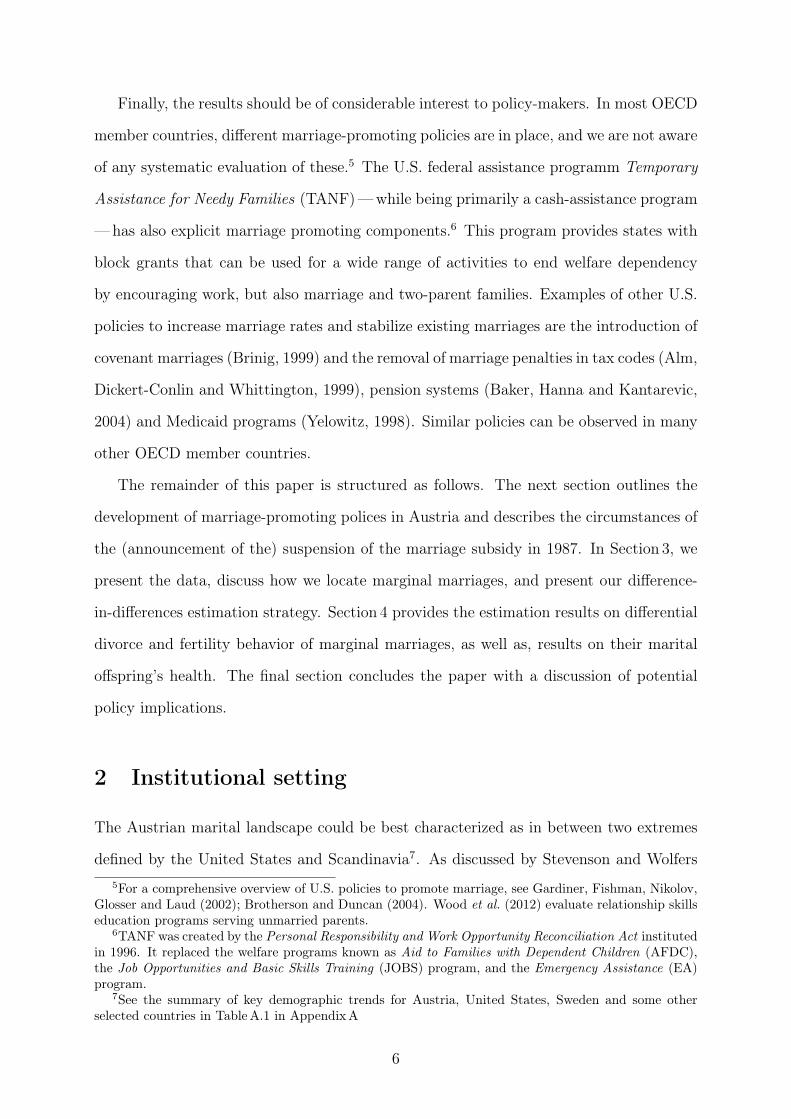
liament in 1971. Over time, the regulations of this marriage subsidy did not change, and

the transfer had not been adjusted for inflation. Almost sixteen years later, on August

26, 1987, the Minister of Finance quite unexpectedly announced the suspension of this

marriage subsidy as of December 31, 1987 without any compensatory schemes.10 The

focus of this paper is on the (announcement of the) suspension of the marriage subsidy.

The announcement of the suspension of the marriage subsidy provided a clear incentive

to marry. Indeed, this led to an enormous marriage boom in the three months from

October to December 1987 (see Figure 1). Compared to the same time period in 1986 (with

7, 844 marriages), we observe an increase of more than 350 percent to 35, 847 marriages

in 1987. Clearly, part of the marriage boom might be simply due to timing; however,

even based on theoretical grounds, we expect an increase in marriage rates to result in a

different selection into marriage.

In a standard family matching model with frictions (Mortensen, 1988), such an unex-

pected announcement decreases the expected present value of a continued search. First,

search costs increase sharply due to the time constraint introduced by the announcement

of the suspension; second, the value of a continued search (for a better match) is reduced

as there are no subsidies after the suspension. Thus, the observed increase in the in-

cidence of marriage in the last quarter of 1987 can be explained by a reduction in the

reservation match quality—that is, in the minimum acceptable match quality sufficient

for a marriage. Marginal marriages are precisely given by those matches that only became

acceptable due to the reduction in the reservation match quality caused by the announce-

ment of the suspension. Consequently, a marginal marriage should be of lower match

quality than average marriages, whose match quality would be sufficient even without

state intervention. In our empirical analysis, we are precisely interested in a quantifi-

cation of this selectivity with respect to marital stability, fertility behavior, and marital

offspring’s health; we refer to this as the selection effect.

A second potential effect of the policy intervention is given by what we term the10See, for instance, Kronen Zeitung on August 27, 1987. The suspension was argued with a necessity

of budget cuts and was quickly enacted without any further parliamentary discussion on October 21,1987. Detailed research of the daily press archives shows that there was also no prior discussion of sucha suspension in the press, nor was there a parliamentary debate before August 1987.

8

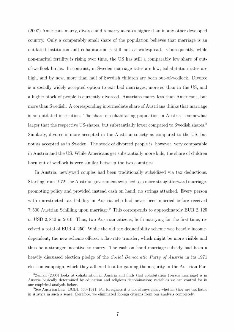
transfer effect. The transfer effect describes the behavioral response due to additional

resources on family outcomes (divorce likelihood and fertility) in the absence of selection:

the true causal effect of the reform.11 Here, one has to keep in mind that the transfer

was just a one-time payment, and the amount (while not negligible) was probably not

significant enough to have long-lasting effects on behavior over time. Therefore, the focus

of our empirical analysis below is on the selection effects; nevertheless, our estimation

strategy also enables us to identify any transfer effects by comparing the period before

the announcement of the suspension with the time period after actual suspension.

3 Estimation strategy and data

We are interested in the differential divorce likelihood and fertility behavior between a

marginal marriage and an average marriage. In other words, we want to learn by how much

a couple who has married just because of a state intervention is on average more (or less)

likely to divorce or to have offspring, compared to a couple who would have married even

without this intervention. We argue that this divorce and fertility gradient is a parameter

that should be taken into account before adopting (costly) marriage-promoting policies,

since a certain level of marital stability and marital offspring is a necessary condition for

pro-marriage policies to succeed.

In our empirical analysis, a marginal marriage is defined as a couple who has married

because of the announcement of the suspension of the marriage subsidy. The suspension

by January 1, 1988 had been implemented without any compensatory measures; it had

been announced abruptly by the Minister of Finance (without any prior discussions) at

the end of August 1987. The suspension thus provides a clear break. The introduction of

the subsidy was not as unexpected. It had been introduced following a heavy discussion

in the 1971 election campaign. Nevertheless, an examination of the introduction allows

us, to provide consistency checks of our main estimation results.11The transfer effect can be highlighted by the following thought experiment. Imagine a situation where

the existence of a marriage subsidy is not publicly announced, but marrying couples (or a sub-group ofthem) still receive a subsidy upon marriage. Here, the transfer effect is given by the difference in thecounterfactual outcomes (with and without subsidy).

9

3.1 Data

For our empirical analysis, we combine information from different administrative data

sources. Most importantly, we use data from the Austrian Marriage Register. This covers

the entirety of marriages and includes the date of marriage, the spouses’ marital histories,

their place of residence, their ages at marriage, their religious denominations and their cit-

izenships. Since 1984, information on the spouses’ countries of birth and on the number,

age and sex of any premarital children is also recorded.12 For further specifications, we

extend our data set with information on the spouses’ labor market statuses and occupa-

tions from the Austrian Social Security Database (ASSD) (see Zweimüller et al., 2009). To

obtain information on marriage duration, we merge the Austrian Divorce Register. Our

base sample consists of all 550, 294 marriages that took place between 1981 and 1993;

thus, we include approximately six years of data before and after the reform. From these

marriages, 150, 767 had divorced by the end of 2007.13 To obtain information on mortality

and out-migration, we matched information from the Austrian Death Register and the

ASSD.14 This results in 36, 893 right-censored observations due to death and 5, 484 due to

out-migration. Finally, for our analysis of fertility behavior and children’s health at birth,

we use data from the Austrian Birth Register on children born to mothers who married

between 1984 and 1993.15 This includes all births in Austria with individual-level infor-

mation on socio-economic characteristics and birth outcomes, such as gestation length,

birth weight, and Apgar scores. Approximately 68 percent of the 401, 314 marriages in

this sample had marital offspring by 2007.12In the mid 1980s about every fifth child was born out of wedlock. This number had increased to

every fourth child by 1995.13No major divorce law reform took place through our sample period. Divorce by mutual consent and

unilateral divorce is available since 1978. Divorce by mutual consent is possible after at least six monthof separation, and unilateral divorce is available after three years apart.

14We presume that if a person is still alive but has no records in the ASSD anymore that s/he leftAustria.

15The reduced sample period is a result of the limited possibility to link the Austrian Marriage Registerwith the Austrian Birth Register before 1984.

10

3.2 Locating marginal marriages

To estimate the selection effect, we need to identify average, early average, and marginal

marriages. While this is impossible at an individual level, our research design allows us

to quantify their aggregate number (over a period of three months). First, we exploit the

fact that only a subset of the population had been eligible for the marriage subsidy, and

we distinguish between three different groups of couples: a comparison group, comprising

couples where no spouse is eligible; a treatment group 1 (T 1), comprising all couples

where one spouse is eligible; and a treatment group 2 (T 2), comprising couples where

both spouses are eligible. That means, spouses from T

2 couples —where both partners

have never been married before— faced the highest incentive to marry; their marriage

had been subsidized in sum with 15, 000 Austrian schillings. T

1 couples comprise one

spouse who had been married before; they received only 7, 500 Austrian schillings. The

comparison group couples consist of spouses who had both been previously married; they

were not eligible for any marriage subsidy.

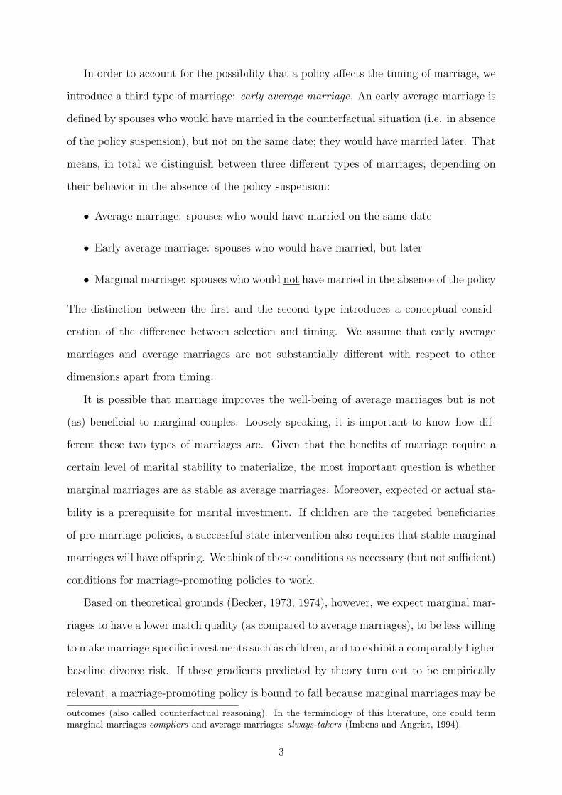
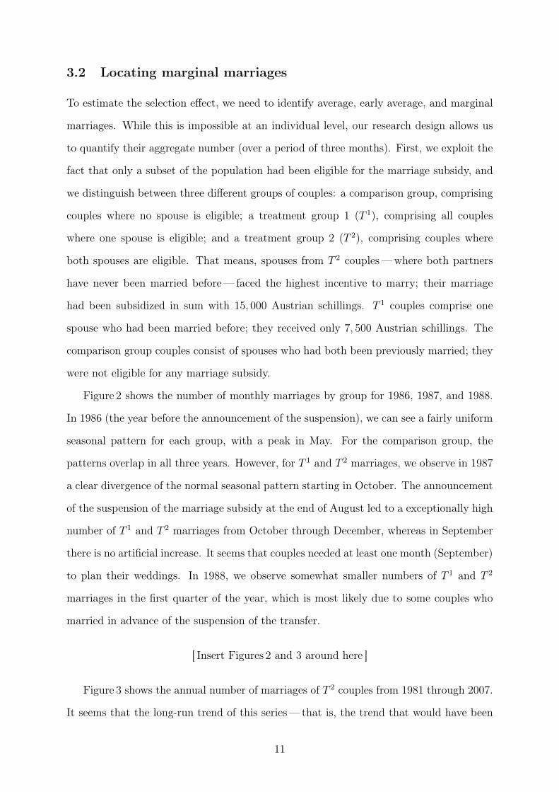
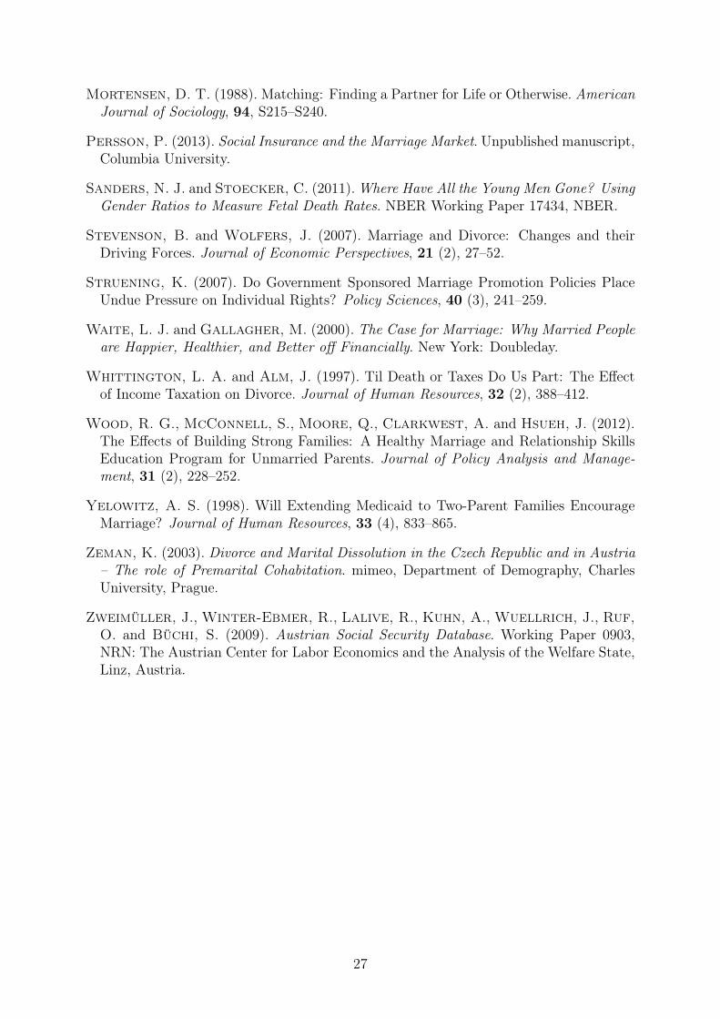
Figure 2 shows the number of monthly marriages by group for 1986, 1987, and 1988.

In 1986 (the year before the announcement of the suspension), we can see a fairly uniform

seasonal pattern for each group, with a peak in May. For the comparison group, the

patterns overlap in all three years. However, for T 1 and T

2 marriages, we observe in 1987

a clear divergence of the normal seasonal pattern starting in October. The announcement

of the suspension of the marriage subsidy at the end of August led to a exceptionally high

number of T 1 and T

2 marriages from October through December, whereas in September

there is no artificial increase. It seems that couples needed at least one month (September)

to plan their weddings. In 1988, we observe somewhat smaller numbers of T

1 and T

2

marriages in the first quarter of the year, which is most likely due to some couples who

married in advance of the suspension of the transfer.

[ Insert Figures 2 and 3 around here ]

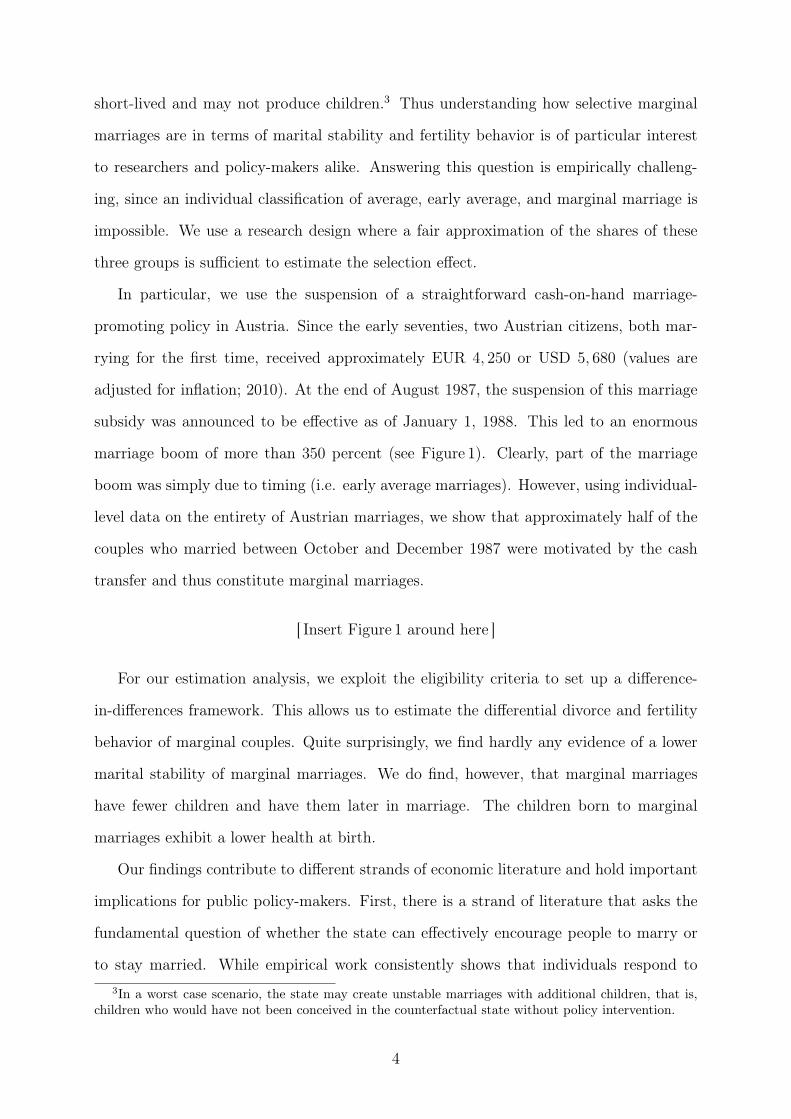
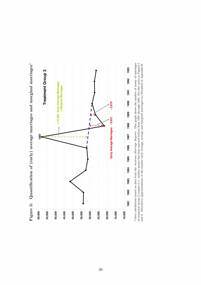
Figure 3 shows the annual number of marriages of T 2 couples from 1981 through 2007.

It seems that the long-run trend of this series — that is, the trend that would have been

11

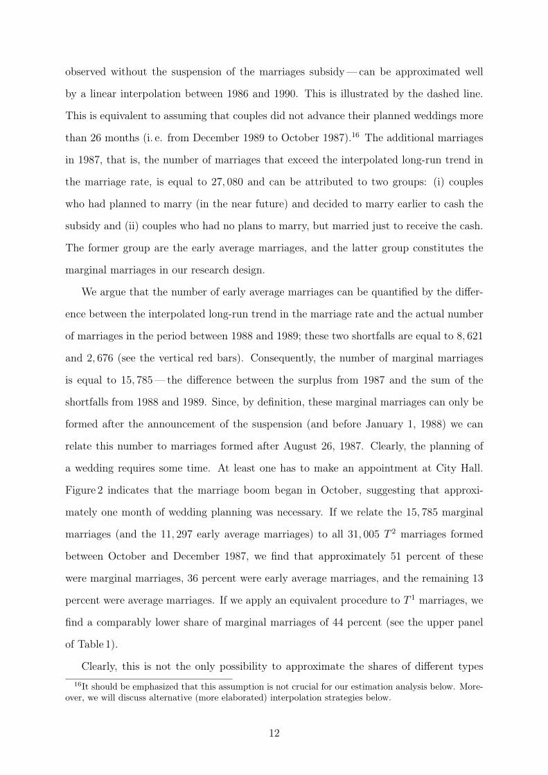
observed without the suspension of the marriages subsidy—can be approximated well

by a linear interpolation between 1986 and 1990. This is illustrated by the dashed line.

This is equivalent to assuming that couples did not advance their planned weddings more

than 26 months (i. e. from December 1989 to October 1987).16 The additional marriages

in 1987, that is, the number of marriages that exceed the interpolated long-run trend in

the marriage rate, is equal to 27, 080 and can be attributed to two groups: (i) couples

who had planned to marry (in the near future) and decided to marry earlier to cash the

subsidy and (ii) couples who had no plans to marry, but married just to receive the cash.

The former group are the early average marriages, and the latter group constitutes the

marginal marriages in our research design.

We argue that the number of early average marriages can be quantified by the differ-

ence between the interpolated long-run trend in the marriage rate and the actual number

of marriages in the period between 1988 and 1989; these two shortfalls are equal to 8, 621

and 2, 676 (see the vertical red bars). Consequently, the number of marginal marriages

is equal to 15, 785—the difference between the surplus from 1987 and the sum of the

shortfalls from 1988 and 1989. Since, by definition, these marginal marriages can only be

formed after the announcement of the suspension (and before January 1, 1988) we can

relate this number to marriages formed after August 26, 1987. Clearly, the planning of

a wedding requires some time. At least one has to make an appointment at City Hall.

Figure 2 indicates that the marriage boom began in October, suggesting that approxi-

mately one month of wedding planning was necessary. If we relate the 15, 785 marginal

marriages (and the 11, 297 early average marriages) to all 31, 005 T

2 marriages formed

between October and December 1987, we find that approximately 51 percent of these

were marginal marriages, 36 percent were early average marriages, and the remaining 13

percent were average marriages. If we apply an equivalent procedure to T

1 marriages, we

find a comparably lower share of marginal marriages of 44 percent (see the upper panel

of Table 1).

Clearly, this is not the only possibility to approximate the shares of different types16It should be emphasized that this assumption is not crucial for our estimation analysis below. More-

over, we will discuss alternative (more elaborated) interpolation strategies below.

12

of marriages. However, alternative procedures give very comparable estimates. In the

Appendix B we present two alternatives in more detail. First, we discuss an alternative

linear approximation based on the period before the announcement of the suspension.

This results in an estimate of 46 percent of marginal marriages and 41 percent of early

average marriages. A more elaborate regression-based approach leads to similar shares of

marginal (45 percent) and early average marriages (38 percent).

[ Insert Table 1 around here ]

Table 1 compares the average characteristics of spouses from the two treatment groups

and the comparison group (who married between October and December) for 1986, 1987,

and 1988. This comparison highlights several things. First we can see that there are

baseline differences between the three groups. As expected, the higher the divorce expe-

rience of the couples is (i. e., moving from T

2 to T

1 and to comparison group marriages),

the older the spouses are, the higher is their age difference, the less likely they are both

Catholic, and the lower is their number of premarital children. Second, as expected, there

is little variation in the composition of the comparison group over time. The only excep-

tion is given by the spouses’ labor market status, which is affected by the business cycle;

in 1987 the unemployment rate was higher than in the other two years. Third, given that

approximately half of the T

1 and T

2 marriage in 1987 were marginal marriages (see upper

panel of Table 1), this comparison should show observable differences between average and

marginal marriages. However, somewhat surprisingly, these numbers suggest that average

and marginal marriages are quite similar along measurable characteristics documented in

the data. For instance, spouses from both groups do not differ significantly in their age or

religious denominations. The only notable difference is the higher incidence of premarital

children among T

1 marriages.

3.3 Difference-in-differences estimation strategy

For our different outcome variables, we use the same specification but different methods

of estimations. To estimate the duration of a marriage, we use Cox proportional hazard

13

models (Cox, 1972), and for the analysis of fertility behavior and marital children’s health

at birth, we use ordinary least squares.

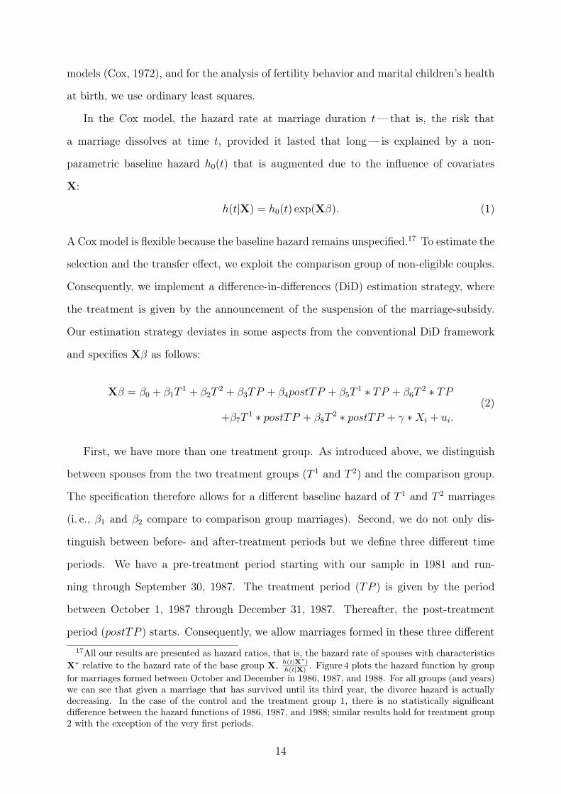
In the Cox model, the hazard rate at marriage duration t—that is, the risk that

a marriage dissolves at time t, provided it lasted that long — is explained by a non-

parametric baseline hazard h0(t) that is augmented due to the influence of covariates

X:

h(t|X) = h0(t) exp(X�). (1)

A Cox model is flexible because the baseline hazard remains unspecified.17 To estimate the

selection and the transfer effect, we exploit the comparison group of non-eligible couples.

Consequently, we implement a difference-in-differences (DiD) estimation strategy, where

the treatment is given by the announcement of the suspension of the marriage-subsidy.

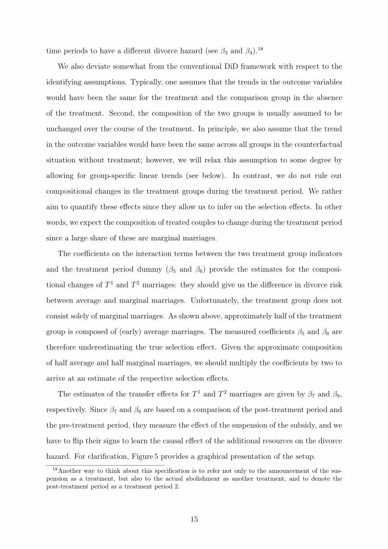
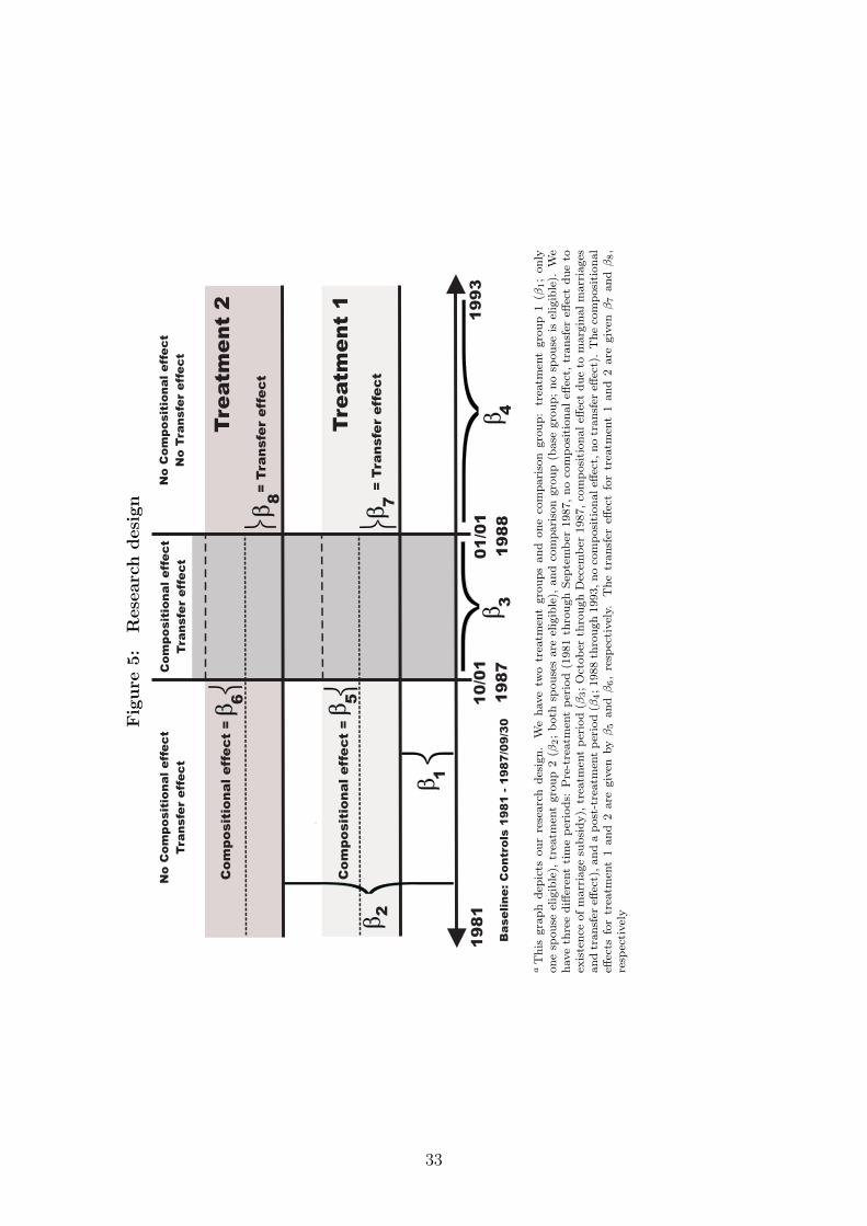
Our estimation strategy deviates in some aspects from the conventional DiD framework

and specifies X� as follows:

X� = �0 + �1T1+ �2T

2+ �3TP + �4postTP + �5T

1 ⇤ TP + �6T2 ⇤ TP

+�7T1 ⇤ postTP + �8T

2 ⇤ postTP + � ⇤Xi + ui.

(2)

First, we have more than one treatment group. As introduced above, we distinguish

between spouses from the two treatment groups (T 1 and T

2) and the comparison group.

The specification therefore allows for a different baseline hazard of T 1 and T

2 marriages

(i. e., �1 and �2 compare to comparison group marriages). Second, we do not only dis-

tinguish between before- and after-treatment periods but we define three different time

periods. We have a pre-treatment period starting with our sample in 1981 and run-

ning through September 30, 1987. The treatment period (TP ) is given by the period

between October 1, 1987 through December 31, 1987. Thereafter, the post-treatment

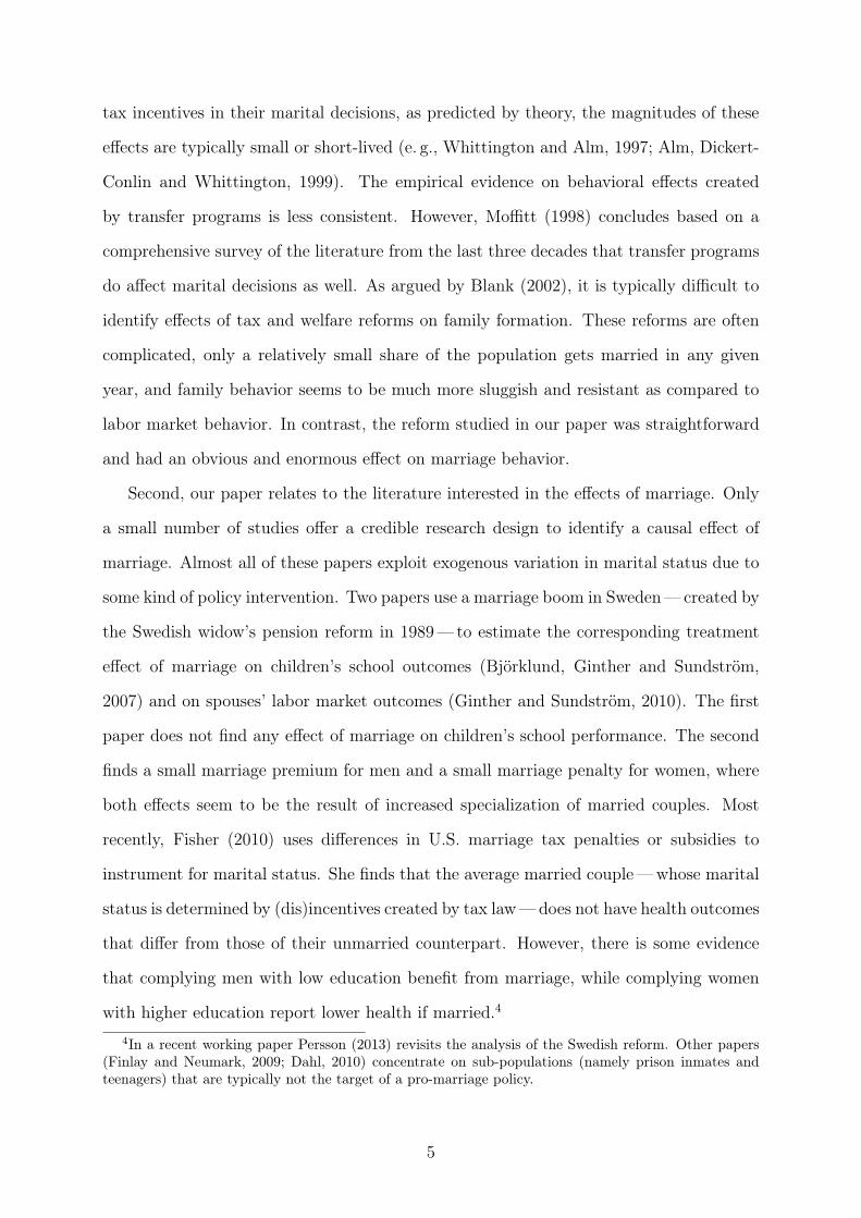
period (postTP ) starts. Consequently, we allow marriages formed in these three different17All our results are presented as hazard ratios, that is, the hazard rate of spouses with characteristics

X⇤ relative to the hazard rate of the base group X, h(t|X⇤)h(t|X) . Figure 4 plots the hazard function by group

for marriages formed between October and December in 1986, 1987, and 1988. For all groups (and years)we can see that given a marriage that has survived until its third year, the divorce hazard is actuallydecreasing. In the case of the control and the treatment group 1, there is no statistically significantdifference between the hazard functions of 1986, 1987, and 1988; similar results hold for treatment group2 with the exception of the very first periods.

14

time periods to have a different divorce hazard (see �3 and �4).18

We also deviate somewhat from the conventional DiD framework with respect to the

identifying assumptions. Typically, one assumes that the trends in the outcome variables

would have been the same for the treatment and the comparison group in the absence

of the treatment. Second, the composition of the two groups is usually assumed to be

unchanged over the course of the treatment. In principle, we also assume that the trend

in the outcome variables would have been the same across all groups in the counterfactual

situation without treatment; however, we will relax this assumption to some degree by

allowing for group-specific linear trends (see below). In contrast, we do not rule out

compositional changes in the treatment groups during the treatment period. We rather

aim to quantify these effects since they allow us to infer on the selection effects. In other

words, we expect the composition of treated couples to change during the treatment period

since a large share of these are marginal marriages.

The coefficients on the interaction terms between the two treatment group indicators

and the treatment period dummy (�5 and �6) provide the estimates for the composi-

tional changes of T 1 and T

2 marriages: they should give us the difference in divorce risk

between average and marginal marriages. Unfortunately, the treatment group does not

consist solely of marginal marriages. As shown above, approximately half of the treatment

group is composed of (early) average marriages. The measured coefficients �5 and �6 are

therefore underestimating the true selection effect. Given the approximate composition

of half average and half marginal marriages, we should multiply the coefficients by two to

arrive at an estimate of the respective selection effects.

The estimates of the transfer effects for T

1 and T

2 marriages are given by �7 and �8,

respectively. Since �7 and �8 are based on a comparison of the post-treatment period and

the pre-treatment period, they measure the effect of the suspension of the subsidy, and we

have to flip their signs to learn the causal effect of the additional resources on the divorce

hazard. For clarification, Figure 5 provides a graphical presentation of the setup.18Another way to think about this specification is to refer not only to the announcement of the sus-

pension as a treatment, but also to the actual abolishment as another treatment, and to denote thepost-treatment period as a treatment period 2.

15

Importantly, for the clean identification of these transfer effects, we have to assume

the absence of any compositional effects prior to the announcement of its suspension. In

order to verify the plausibility of this assumption we examine the introduction of the

marriage subsidy in the year 1972. Based on a comparable DiD framework we do not

find any evidence for compositional effects induced by the introduction of the subsidy. A

detailed discussion and estimation output is provided in Appendix C. This finding seems

quite intuitive. Until 1986 Austrians were used to ongoing marriage-promoting policies

and there was not a strong incentive to risk a bad marriage, if one could also have

waited for the right spouse to arrive and to cash the subsidy later. In contrast, after the

announcement of the suspension, the incentives have changed substantially and we would

expect compositional effects during the defined treatment period.

[ Insert Figures 4 and 5 around here ]

In each of our specifications, we control for quarter fixed-effects, district fixed-effects,

and group specific time trends. The latter relax to some degree the parallel trend assump-

tion. Our baseline specification also includes the wife’s age, the spouses’ age difference

(squared), and the spouses’ religious denominations at the time of marriage as covariates.

With respect to religious denomination, we differentiate between the three quantitatively

most important religious affiliations in Austria: Catholic (73.6 percent), no religious de-

nomination (12.0 percent), and others (14.4 percent) (Austrian Census from 2001). This

gives rise to six possible combinations, where a marriage between two Catholics will serve

as the base group. Given that we are interested in the estimation of compositional effects,

more control variables are not necessarily better; they may partial out some of these ef-

fects. Still, we present a further specification in which we also control for the spouses’

labor market statuses and occupations (measured one quarter before marriage) and the

number of joint pre-marital children; where the latter information is only available starting

from 1984.19 The results do not change much after including further covariates.20

19Frimmel, Halla and Winter-Ebmer (2013) show for Austria that a lower age at marriage, differentreligious denominations, and the presence of premarital children are associated with a higher risk ofdivorce.

20Clearly, we do not want to control for any post-marriage events. It can be argued that all other

16

An equivalent set of specifications, but using least squares regression, is used for the

estimation of marital fertility behavior and marital offspring’s health at birth. In the

latter case the set of covariates is adjusted somewhat (see below).

4 Estimation results

At first, we present our estimation results on marital instability. Section 4.2 provides

our estimates on differential fertility behavior, and Section 4.3 reports results on marital

offspring’s health at birth.

4.1 Marital instability

Table 2 summarizes our main estimation results on marital stability using different specifi-

cations. In contrast to theoretical predictions, we find practically no evidence for a higher

divorce risk of marginal marriages compared to average marriages. This finding is very

consistent across different specifications. In the baseline specification in column (I), we

include all marriages. In the second and the third specification, we restrict our sample,

to exclude potentially selected marriages from our comparison group, which may bias our

estimates of the composition (and selection) effect downward. In particular, in specifi-

cation (II) we exclude marriages formed in 1983. In this year the Austrian government

announced the abolishment of the tax deductibility of dowry per January 1, 1984. Thus,

our comparison group in 1983 may comprise couples who married to save taxes and who

would not have married (at that time) without this reform (see the spike in Figure 1).

In specification (III) we further exclude marriages formed immediately after the reform

(i. e., in the first half year of 1988). Given that a sizable number of spouses have brought

forward their wedding day to cash the subsidy (the early average marriages), the pool

of marriages formed in early 1988 might also be selective. In the fourth and in the fifth

specification, we extend the set of socio-demographic control variables. Specification (IV)

factors that might also have an important impact on divorce risk—such as the number of post-maritalchildren, the labour supply of either partner and marital satisfaction — are endogenous with respect tothe viability of the marriage, and therefore all coefficient estimates might be biased.

17

also includes information on the spouses’ labor market statuses and occupations (mea-

sured in the quarter before marriage). Specification (V) also controls for the number of

pre-marital children.

[ Insert Table 2 around here ]

Across specifications, we consistently find no statistically significant composition ef-

fects. The point estimates (for both groups) are quite small and insensitive to modifi-

cations of the sample and the covariates included. Even leaving statistical significance

aside, the point estimates of the composition effects provide little to no evidence for a

different marital instability of marginal marriages. In the case of T 1, the point estimates

even suggest a lower divorce likelihood for marginal marriages. For T

2, we find posi-

tive composition effects between 2.8 and 3.6 percent. However, the lowest p-value (see

T

2 in specification II) is 0.17 and, therefore, far above conventional levels of statistical

significance.

Given that during the treatment period TP the groups of T 1 and T

2 marriages con-

sisted approximately half of marginal marriages — and half of (early) average marriages —

we can multiply our estimates of the compositional effects by two to arrive at an appro-

priate estimate of the selection effect. Assuming point estimates that are twice as large

as the ones we have estimated, only one out of our ten estimates in Table 2 would reach

significance levels close to conventional levels (8.6 in specification II).

To sum up, a conservative interpretation of the estimation of the compositional effects

is that there is only little evidence that marginal marriages are a selected group in terms

of marital stability. This leaves us with the somewhat surprising result that marriage-

promoting policies indeed have the potential to create stable marriages.

Less surprisingly, there is also little evidence for transfer effects. Only in the case of

specification (V) we do find a statistically significant transfer effect for T 2 marriages. The

point estimate suggests that their divorce likelihood decreased by 5.4 percent due to the

marriage subsidy. The effect is, however, not statistically significant at the five percent

level.

18

The remaining control variables from our DiD specification show that our treated

couples — basically individuals in their first marriages — have significantly lower hazard

rates. The lowest divorce risk is observed for spouses who are both in their first marriage

(see �2), which is well known from the literature. More importantly, our controls for

the treatment period (�3) and the post-treatment period (�4) are always statistically

indistinguishable from one showing that there are no other time trends that might interfere

with our compositional effects.

4.2 Marital fertility

In this section, we report estimation results on fertility behavior. Table 3 summarizes DiD

estimation results for which we consider the number of marital children born by 2007 as

an outcome variable.21 While not all women in our sample have reached the end of their

reproductive life by 2007, our estimation results will most likely resemble the effect on

completed fertility since the vast majority of women are born before 1968.22 We only

list results for our most extensive specifications— resembling Specifications (IV) and (V)

from Table 2 —since the results do not change much across other specifications.

[ Insert Table 3 and Figure 6 around here ]

In contrast to the results on marital instability, we find statistically significant composi-

tional effects with respect to fertility behavior. Specification (I) suggests that T 2 marriages

formed during the treatment period have less marital offspring (minus 0.15 children). For

T

1 marriages, we observe a comparably smaller effect of minus 0.06 children. Thus, the

selection effects for T

2 and T

1 marriages are approximately minus 0.30 and minus 0.12

children. This is equivalent to 25 and 10 percent fewer marital offspring for T

2 and T

1

marriages, respectively.

Part of these effects, however, might be due to the fact that marginal marriages tend

to have more pre-marital children. Specification (II) introduces the number of pre-marital21We use the definition of marital children from the Austrian Birth Register, where a child is coded as

a marital child if the mother was married at any time during pregnancy.22Thus, by 2007 approximately 80 percent of the women in our sample are 40 years of age or older.

19

children as an additional control variable. Indeed, the statistical significance of the com-

positional effect for T 1 marriages vanishes, and the point estimate is essentially zero. This

suggests that marginal marriages from T

1 have the same number of overall children (as

average marriages), but marginal marriages are more likely to have some of them born

out of wedlock. In the case of T 2 marriages, the estimated effect stays statistically sig-

nificant, but shrinks somewhat in size. This results in a reduced selection effect of minus

0.21 children or 17 percent fewer marital offspring. In other words, marginal marriages of

T

2 are statistically significantly different compared to average marriages in terms of their

overall number of children.

Again, there is only limited evidence for any transfer effects. While �8 is statistically

significant in the first specification, all transfer effects in the second specification are

statistically insignificant.

Figure 6 provides further results to explore potentially differential timing of marital

fertility. The bars summarize estimates of compositional effects in terms of the number of

marital children by marriage duration, and they reveal a diverging timing for marriages

formed during the treatment period. This translates into the following estimates of selec-

tion effects. For marginal marriages from both treatment groups, we observe statistically

significant fewer marital offspring in the first two years of marriage (T 1: minus 0.1 chil-

dren, T 2: minus 0.24 children). In the case of T 1 couples, we observe positive selection

effects thereafter. In sum, after 15 years of marriage, marginal marriages from T

1 have

the same number of marital offspring as average marriages. In contrast, in the case of T 2

couples, we find little evidence for a catching-up process, and the difference prevails over

15 years of marriage. In particular, the difference after two years of marriage and fifteen

years of marriage is very small — which can be seen by comparing the bar on the far left

and the one on the far right.23

In sum, these results suggest that marginal marriages (of T 2) have fewer children and

have them later in marriage (this applies to T

1 and T

2 couples).23In a further estimation, we examined the extensive marital fertility margin. We find that marginal

marriages are approximately four (T 1) and six (T 2) percent more likely to have no marital offspring atall (measured in the year 2007).

20

4.3 Children’s health at birth

Before we turn to our estimations of children’s health at birth it should be noted that

Austria has a Bismarckian (social) health insurance system with almost universal access

to high quality health care. While Austria has a free of charge mother-child healthcare

examination program — that comprises a series of pre- and post-natal check-ups — already

since 1974, infant mortality was still quite high in the 1980s. It amounted to eleven deaths

of infants under the age of one year per 1,000 live births; which was equal to the rate of the

US. Since then infant mortality rates declined but are still significantly higher compared

to Scandinavian countries (see Table A.1 in AppendixA).

To compare the health of marital children born to marginal and average marriages, we

use data provided in the Austrian Birth Register on the gestation length, birth weight,

Apgar scores and sex of the first marital child.24 These are the most common measures

of health at birth. Gestation periods are classified as premature if they are below 37

weeks. Weight at birth is typically considered as low if it is below 2500 grams, and very

low below 1500 grams. Both a premature gestation length and a low birth weight are

related to higher likelihood of infant mortality, but may also have long lasting effects on

health, education, and labor market outcomes later in life (see, for instance, Behrman

and Rosenzweig, 2004; Black, Devereux and Salvanes, 2007; Almond and Currie, 2011).

The Apgar scores assess after one, five, and ten minutes quickly and summarily the

health of newborn babies based on five criteria (appearance, pulse, grimace, activity, and

respiration) and range from zero (“good”) to ten (“bad”). Finally, the likelihood of a male

birth serves as a metric of fetal death. This indicator exploits the fact that males are more

sensitive than females to negative health shocks in utero (Sanders and Stoecker, 2011).25

[ Insert Table 4 around here ]

The estimation results from a DiD estimation are summarized in Table 4. We do not

find any statistically significant composition effects based on gestational length, Apgar24It has to be noted that marginal marriages have somewhat fewer children, and have them later in

life. We take the latter fact into account by including mother’s age at birth as a control variable.25The exact mechanism behind this culling process is still unclear. Still researchers in different fields

agree that the sex-ratio is a useful proxy for early spontaneous abortions (Catalano and Bruckner, 2006;Almond and Edlund, 2007).

21

scores or the sex indicator.26 However, we find significant evidence in the case of birth

weight. The point estimates for both treatment groups suggest compositional effects of

approximately minus ninety grams. Given potential misclassifications in the marginal

marriages (as discussed above) we might multiply this effect by the factor two. The

resulting selection effect is equivalent to approximately minus 5.5 percent or approximately

one third of a sample standard deviation. This quantitative effect importance of this effect

is moderate. However, if we use an indicator for low birth weight (equal to one below

2500 grams, and zero otherwise) as an alternative outcome variable, we find substantially

larger effects. Untabulated regressions show that newborns from a marginal marriage

are at least between 3.8 (T1) and 5.0 (T2) percentage points more likely to have a low

birth weight. The fact that the estimated effects are quantitatively more important based

on the indicator variables (as compared to the birth weight) shows that the composition

effects are centered in the lower tail of the birth weight distribution. Put differently,

among the marginal marriages there are some couples whose offspring has very low birth

endowment. Equivalent results are obtained for more parsimonious specifications.

The remaining variables from the DiD specification are almost all statistically insignifi-

cant. Children born to parents where one spouse (see �1) or two spouses (see �2) had been

married before are as healthy as children born to parents in their first marriage. Further,

children born to control parents in the treatment period (see �3) and in the post-treatment

period (see �4) are indistinguishable from those control children born in the pre-treatment

period. Finally, we do not find any evidence for transfer effects on children’s health at

birth. The untabulated estimated effects of the socio-economic controls variables are very

comparable to those found in other papers (e. g., Frimmel and Pruckner, 2013).

4.4 Robustness checks

We ran several robustness checks to test the sensitivity of our results which are summarized

in AppendixD. For instance, we excluded the group-specific time trends from all our

specifications (see TablesD.1 to D.3). We also extended our sample period and used all26The same is true for a binary indicator capturing premature birth.

22

marriage cohorts from 1974 through 2000 (see Tables D.4 to D.6). Overall, we do not find

any significant changes in the estimated compositional and transfer effects due to these

modifications. This applies to all outcomes under consideration.

5 Conclusions and policy implications

We exploit a unique policy episode in Austria, where a suspension of a relatively large

marriage subsidy was announced, and the number of marriages was rapidly increasing

by 350 percent just before this suspension. This allows us to locate couples who mar-

ried just because of the suspension. We examine the selectivity of these marginal mar-

riages —couples who would not have married in the counterfactual situation without the

suspension —within a difference-in-differences framework along the outcome dimensions

of marital stability, fertility behavior, and marital offspring’s health. In particular, the

estimation of compositional effects of the treated population due to the announcement of

the suspension allows us to quantify the degree of selectivity. Contrary to expectations,

we find that those who married just because of the subsidy are not different from the

average marriages in terms of marital stability. However, they have somewhat fewer chil-

dren and have them later in their marriage. It also has to be noted that their offspring is

less healthy at birth.

Thus, it seems that—at least in this case — pro-marriage policies can work. Finan-

cial incentives significantly influence marriage behavior, and those who marry because of

the subsidy are not much different from an average marriage. The concern that marginal

marriages are less stable — and may even generate additional children affected by parental

divorce —proves to be unfounded. However, we have also evidence showing that simply

motivating couples to marry does not improve all their family outcomes; health outcomes

of children born to marginal marriages are still worse compared to those of average mar-

riages.

Clearly, these results have to be interpreted in the light of the Austrian institutional

setting and its specific marital landscape. We would think of Austria as a country with

attitudes towards marriage and divorce in the middle of the spectrum between the USA

23

and, say, Scandinavia. Moreover, it is a representative example for a Central European

welfare state. In countries with a less pronounced social insurance system marginal and

average marriages may be more distinct and the generalizability of our results may be

limited.

Whether it is worthwhile — from a taxpayer’s point of view—to invest money into

inducing people to get married is another issue. The existing evidence indicates that causal

effects of marriage are quite mixed. In particular, instrumental variables estimates of local

average treatment effects may vary substantially across different groups of compliers and,

therefore, across different groups of persons induced into marriage.27 To evaluate pro-

marriage policies further, estimates of local average treatment effects precisely for the

population responding to pro-marriage policies (i. e., compliers) are needed. We hope

further evidence from such instrumental variable approaches will be available soon. Our

results — which are based on a subsidy that induced a relatively large shift in marriage

behavior— suggest that the local average treatment effects provided by such instrumental

variables approaches may also be good approximations for the average treatment effects

since marginal marriages are quite comparable to average marriages.

Our results suggest that the match quality of marginal marriages is almost sufficient

to warrant a stable marriage. One might expect then that a substantially higher subsidy

would reduce the marginal reservation match quality further and result in a higher degree

of negative selection. Consequently, pro-marriage policies should not incorporate too

high incentives, after all. Furthermore, policy makers could try not to simply subsidize

marriage, but to facilitate stable marriage by, for instance, subsidizing marital-specific

investment.

27See, for instance Ichino and Winter-Ebmer (1999) for a study in which different instruments shiftdifferent populations and therefore lead to different conclusions.

24

References

Alm, J., Dickert-Conlin, S. and Whittington, L. A. (1999). Policy Watch: TheMarriage Penalty. Journal of Economic Perspectives, 13 (3), 193–204.

Almond, D. and Currie, J. (2011). Killing Me Softly: The Fetal Origins Hypothesis.Journal of Economic Perspectives, 25 (3), 153–172.

— and Edlund, L. (2007). Trivers-Willard at Birth and One Year: Evidence fromUS Natality Data 1983–2001. Proceedings of the Royal Society B: Biological Sciences,274 (1624), 2491–2496.

Amato, P. R. (2007a). Response to Furstenberg. Journal of Policy Analysis and Man-agement, 26 (4), 961–962.

— (2007b). Strengthening Marriage is an Appropriate Social Policy Goal. Journal ofPolicy Analysis and Management, 26 (4), 952–955.

Baker, M., Hanna, E. and Kantarevic, J. (2004). The Married Widow: MarriagePenalties Matter! Journal of the European Economic Association, 2 (4), 634–664.

Becker, G. S. (1973). A Theory of Marriage: Part I. Journal of Political Economy,81 (4), 813–846.

— (1974). A Theory of Marriage: Part II. Journal of Political Economy, 82 (2), S11–S26.

Behrman, J. R. and Rosenzweig, M. R. (2004). Returns to Birthweight. Review ofEconomics and Statistics, 86 (2), 586–601.

Björklund, A., Ginther, D. K. and Sundström, M. (2007). Does Marriage Matterfor Children? Assessing the Causal Impact of Legal Marriage. IZA Discussion Papers3189, Institute for the Study of Labor (IZA).

Black, S. E., Devereux, P. J. and Salvanes, K. G. (2007). From the Cradle to theLabor Market? The Effect of Birth Weight on Adult Outcomes. Quarterly Journal ofEconomics, 122 (1), 409–439.

Blank, R. M. (2002). Evaluating Welfare Reform in the United States. Journal of Eco-nomic Literature, 40 (4), 1105–1166.

Brinig, M. F. (1999). Economics, Law, and Covenant Marriage. Gender Issues, 16 (1–2),4–33.

Brotherson, S. E. and Duncan, W. C. (2004). Rebinding the Ties That Bind: Gov-ernment Efforts to Preserve and Promote Marriage. Family Relations, 53 (5), 459–468.

Catalano, R. and Bruckner, T. (2006). Secondary Sex Ratios and Male Lifespan:Damaged or Culled Cohorts. Proceedings of the National Academy of Sciences, 103 (5),1639–1643.

Cherlin, A. J. (2003). Should the Government Promote Marriage? Contexts, 2 (4),22–29.

25

Cox, D. R. (1972). Regression Models and Life-Tables. Journal of the Royal StatisticalSociety: Series B (Methodological), 34 (2), 187–220.

Dahl, G. (2010). Early Teen Marriage and Future Poverty. Demography, 47 (3), 689–718.

Finlay, K. and Neumark, D. (2009). Is Marriage Always Good for Children? Evidencefrom Families Affected by Incarceration. Journal of Human Resources, 45 (4), 1046–1088.

Fisher, H. (2010). Just a Piece of Paper? The Health Benefits of Marriage. Unpublishedmansucript, University of Sydney.

Frimmel, W., Halla, M. and Winter-Ebmer, R. (2013). Assortative Mating andDivorce: Evidence from Austrian Register Data. Journal of the Royal Statistical SocietySeries A.

— and Pruckner, G. J. (2013). Birth Weight and Family Status Revisited: Evidencefrom Austrian Register Data. Health Economics.

Furstenberg, F. F. (2007a). Response to Amato. Journal of Policy Analysis and Man-agement, 26 (4), 963–964.

— (2007b). Should Government Promote Marriage? Journal of Policy Analysis and Man-agement, 26 (4), 956–960.

Gardiner, K. N., Fishman, M. E., Nikolov, P., Glosser, A. and Laud, S. (2002).State Policies to Promote Marriage – Final Report. Tech. rep., U.S. Department ofHealth and Human Services Assistant Secretary for Planning and Evaluation, Wash-ington, DC.

Ginther, D. K. and Sundström, M. (2010). Does Marriage Lead to Specialization?An Evaluation of Swedish Trends in Adult Earnings Before and After Marriage. mimeo,University of Kansas and Stockholm University.

Halla, M., Lackner, M. and Scharler, J. (2013). Does the Welfare State Destroythe Family? Evidence from OECD Member Countries. IZA Discussion Papers 7210,Institute for the Study of Labor (IZA), Bonn.

Ichino, A. and Winter-Ebmer, R. (1999). Lower and Upper Bounds of Returns toSchooling, An Exercise in IV Estimation with Different Instruments. European Eco-nomic Review, 43, 889–901.

Imbens, G. W. and Angrist, J. D. (1994). Identification and Estimation of LocalAverage Treatment Efffects. Econometrica, 62 (2), 467–475.

Matouschek, N. and Rasul, I. (2008). The Economics of the Marriage Contract:Theories and Evidence. Journal of Law and Economics, 51 (1), 59–110.

McLanahan, S. (2007). Should Government Promote Marriage? Journal of Policy Anal-ysis and Management, 26 (4), 951.

Moffitt, R. A. (1998). Welfare, the Family, and Reproductive Behavior: Research Per-spectives, Washington: National Academies Press, chap. The Effect of Welfare on Mar-riage and Fertility, pp. 50–97.

26

Mortensen, D. T. (1988). Matching: Finding a Partner for Life or Otherwise. AmericanJournal of Sociology, 94, S215–S240.

Persson, P. (2013). Social Insurance and the Marriage Market. Unpublished manuscript,Columbia University.

Sanders, N. J. and Stoecker, C. (2011). Where Have All the Young Men Gone? UsingGender Ratios to Measure Fetal Death Rates. NBER Working Paper 17434, NBER.

Stevenson, B. and Wolfers, J. (2007). Marriage and Divorce: Changes and theirDriving Forces. Journal of Economic Perspectives, 21 (2), 27–52.

Struening, K. (2007). Do Government Sponsored Marriage Promotion Policies PlaceUndue Pressure on Individual Rights? Policy Sciences, 40 (3), 241–259.

Waite, L. J. and Gallagher, M. (2000). The Case for Marriage: Why Married Peopleare Happier, Healthier, and Better off Financially. New York: Doubleday.

Whittington, L. A. and Alm, J. (1997). Til Death or Taxes Do Us Part: The Effectof Income Taxation on Divorce. Journal of Human Resources, 32 (2), 388–412.

Wood, R. G., McConnell, S., Moore, Q., Clarkwest, A. and Hsueh, J. (2012).The Effects of Building Strong Families: A Healthy Marriage and Relationship SkillsEducation Program for Unmarried Parents. Journal of Policy Analysis and Manage-ment, 31 (2), 228–252.

Yelowitz, A. S. (1998). Will Extending Medicaid to Two-Parent Families EncourageMarriage? Journal of Human Resources, 33 (4), 833–865.

Zeman, K. (2003). Divorce and Marital Dissolution in the Czech Republic and in Austria– The role of Premarital Cohabitation. mimeo, Department of Demography, CharlesUniversity, Prague.

Zweimüller, J., Winter-Ebmer, R., Lalive, R., Kuhn, A., Wuellrich, J., Ruf,O. and Büchi, S. (2009). Austrian Social Security Database. Working Paper 0903,NRN: The Austrian Center for Labor Economics and the Analysis of the Welfare State,Linz, Austria.

27

6Tables

&figures

Fig

ure

1:A

nnu

alnu

mber

ofm

arri

ages

and

div

orce

sper

1,00

0of

pop

ula

tion

,A

ust

ria

1960

thro

ugh

2009

a

1983

1972

1987

01234567891011

1960

1964

1968

1972

1976

1980

1984

1988

1992

1996

2000

2004

2008

Number of cases per 1,000 population

Mar

riage

sD

ivor

ces

aO

wn

calc

ulat

ions

base

don

data

from

Statistics

Austria;de

tails

are

avai

labl

eup

onre

ques

t.N

ote,

per

Dec

embe

r31

,19

71th

ede

duct

abili

tyof

furn

ishi

ngs

and

arti

cles

ofda

ilyus

eup

to70

,000

Aus

tria

nsc

hilli

ngw

ithi

nth

efir

stfiv

eye

ars

afte

rth

ees

tabl

ishm

ent

ofa

new

hous

ehol

dby

new

lyw

eds

was

abol

ishe

d.H

owev

er,

per

Janu

ary

1,19

72a

mar

riag

esu

bsid

yfo

rev

ery

pers

onw

ith

unre

stri

cted

tax

liabi

lity

inA

ustr

ian

who

had

neve

rbe

enm

arri

edof

7,50

0A

ustr

ian

schi

lling

was

intr

oduc

ed.

Tha

tm

eans

,tw

oA

ustr

ian

citi

zens

,bo

thm

arry

ing

the

first

tim

e,re

ceiv

eda

tota

lof

15,0

0A

ustr

ian

schi

lling

(201

0:E

UR

4,25

0or

USD

5,68

0).

Per

Janu

ary1,

1984

the

tax

dedu

ctib

ility

ofdo

wry

was

abol

ishe

d.Per

Dec

embe

r31

,198

7th

em

arri

age

subs

idy

was

susp

ende

dw

itho

utan

yre

plac

emen

t.T

his

was

anno

unce

don

Aug

ust26

,198

7.

28

Figure 2: Monthly number of marriages by group in the years 1986 to 1988a

Ŧ1

Ŧ.5

0

.5

1

1.5

1 2 3 4 5 6 7 8 9 10 11 12

Treatment Group 2

Ŧ1

Ŧ.5

0

.5

1

1.5

1 2 3 4 5 6 7 8 9 10 11 12

Treatment Group 1

Ŧ1

Ŧ.5

0

.5

1

1.5

1 2 3 4 5 6 7 8 9 10 11 12

Comparison Group

Month of marriage

1986 1987 1988

a Own calculations based on data from the Austrian Marriage Register. These graphs show the number ofmonthly marriages for three groups (see below) in the years in 1986, 1987 and 1988. The monthly numberof marriages is normalized to May of each year (and group). Treatment group 2 comprises couples whereeach spouse has never been married before. Treatment group 1 consists of couples where only one spousehas been married before. The comparison group covers couples where both spouse had been married before.

29

Fig

ure

3:Q

uan

tifica

tion

of(e

arly

)av

erag

em

arri

ages

and

mar

ginal

mar

riag

esa

10,0

00

15,0

00

20,0

00

25,0

00

30,0

00

35,0

00

40,0

00

45,0

00

50,0

00

55,0

00

60,0

00

1981

1982

1983

1984

1985

1986

1987

1988

1989

1990

1991

1992

1993

Early

Ave

rage

Mar

riage

s:

Trea

tmen

t Gro

up 2

1987

+ 2

7,08

0 E

arly

Ave

rage

Mar

riage

s

+

Mar

gina

l Mar

riage

s

- 2,6

76- 8

,621

aO

wn

calc

ulat

ions

base

don

data

from

the

Austrian

Marriage

Register.

Thi

sgr

aph

show

sth

enu

mbe

rof

year

lyof

mar

riag

esof

trea

tmen

tgr

oup2

coup

les

(i.e

.ne

ithe

rsp

ouse

has

been

mar

ried

befo

re)

from

1981

thro

ugh19

93.

See

also

note

sto

Fig

ures

1an

d2.

Alt

erna

tive

appr

oxim

atio

nsof

the

num

ber

earl

yav

erag

e,av

erag

ean

dm

argi

nalm

arri

ages

are

disc

usse

din

App

endi

xB

.

30

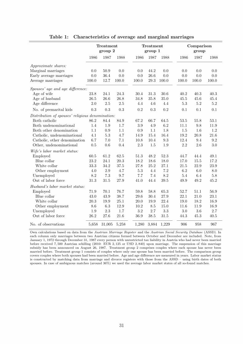
Table 1: Characteristics of average and marginal marriages

Treatment Treatment Comparison

group 2 group 1 group

1986 1987 1988 1986 1987 1988 1986 1987 1988

Approximate shares:Marginal marriages 0.0 50.9 0.0 0.0 44.2 0.0 0.0 0.0 0.0Early average marriages 0.0 36.4 0.0 0.0 26.6 0.0 0.0 0.0 0.0Average marriages 100.0 12.7 100.0 100.0 29.3 100.0 100.0 100.0 100.0

Spouses’ age and age difference:Age of wife 23.8 24.1 24.3 30.4 31.3 30.6 40.2 40.3 40.3Age of husband 26.5 26.6 26.8 34.8 35.8 35.0 45.5 45.6 45.4Age difference 2.0 2.5 2.5 4.4 4.6 4.4 5.3 5.2 5.2

No. of premarital kids 0.3 0.3 0.3 0.2 0.3 0.2 0.1 0.1 0.1

Distribution of spouses’ religious denomination:Both catholic 86.2 84.4 84.9 67.2 66.7 64.5 53.5 55.8 53.1Both undenominational 1.4 1.9 1.7 3.9 4.9 6.2 11.1 9.8 11.9Both other denomination 1.1 0.9 1.1 0.9 1.1 1.8 1.5 1.6 1.2Catholic, undenominational 4.1 5.3 4.7 14.9 15.4 16.4 19.2 20.8 21.6Catholic, other denomination 6.7 7.0 7.1 10.8 10.4 9.3 12.4 9.4 9.2Other, undenominational 0.5 0.6 0.4 2.3 1.5 1.9 2.2 2.6 3.0

Wife’s labor market status:Employed 60.5 61.2 62.5 51.3 48.2 52.3 44.7 44.4 49.1

Blue collar 23.2 24.1 20.3 18.2 18.6 18.0 17.0 15.5 17.2White collar 33.3 34.2 37.5 27.8 25.2 27.1 21.5 22.9 23.9Other employment 4.0 2.9 4.7 5.3 4.4 7.2 6.2 6.0 8.0

Unemployed 8.2 7.3 9.7 7.7 7.4 8.2 5.4 6.4 5.8Out of labor force 31.3 31.5 27.9 41.0 44.4 39.5 49.9 49.2 45.2

Husband’s labor market status:Employed 71.9 70.1 76.7 59.8 58.8 65.3 52.7 51.1 56.9

Blue collar 43.0 43.9 38.7 29.6 30.4 27.9 22.1 21.0 23.1White collar 20.3 19.9 25.1 20.0 19.9 22.4 19.0 18.2 16.9Other employment 8.6 6.3 12.9 10.2 8.5 15.0 11.6 11.9 16.9

Unemployed 1.9 2.3 1.7 3.2 2.7 3.3 3.0 3.6 2.7Out of labor force 26.2 27.6 21.6 36.9 38.5 31.5 44.3 45.3 40.5

No. of observations 5,658 31,005 5,258 1,280 3,884 1,229 906 958 967

Own calculations based on data from the Austrian Marriage Register and the Austrian Social Security Database (ASSD). Ineach column only marriages between two Austrian citizens formed between October and December are included. Note, fromJanuary 1, 1972 through December 31, 1987 every person with unrestricted tax liability in Austria who had never been marriedbefore received 7, 500 Austrian schilling (2010: EUR 2, 125 or USD 2, 840) upon marriage. The suspension of this marriagesubsidy has been announced on August 26, 1987. Treatment group 2 comprises couples where each spouse has never beenmarried before. Treatment group 1 consists of couples where only one spouse has been married before. The comparison groupcovers couples where both spouses had been married before. Age and age difference are measured in years. Labor market statusis constructed by matching data from marriage and divorce registers with those from the ASSD – using birth dates of bothspouses. In case of ambiguous matches (around 36%) we used the average labor market states of all so-found matches.

31

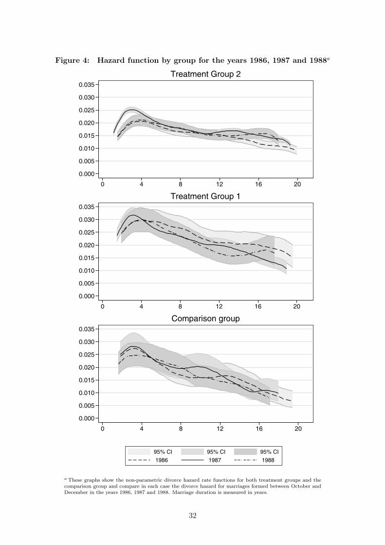
Figure 4: Hazard function by group for the years 1986, 1987 and 1988a

0.000

0.005

0.010

0.015

0.020

0.025

0.030

0.035

0 4 8 12 16 20

Treatment Group 2

0.000

0.005

0.010

0.015

0.020

0.025

0.030

0.035

0 4 8 12 16 20

Treatment Group 1

0.000

0.005

0.010

0.015

0.020

0.025

0.030

0.035

0 4 8 12 16 20

Comparison group

95% CI 95% CI 95% CI 1986 1987 1988

a These graphs show the non-parametric divorce hazard rate functions for both treatment groups and thecomparison group and compare in each case the divorce hazard for marriages formed between October andDecember in the years 1986, 1987 and 1988. Marriage duration is measured in years.

32

Fig

ure

5:R

esea

rch

des

ign

10/0

1

1987

01/0

1

1988

1981

1993

Tre

atm

ent

2

No

Com

posit

ionaleff

ect

No

Tra

nsfe

reff

ect

No

Com

posit

ionaleff

ect

Tra

nsfe

reff

ect

Com

posit

ionaleff

ect

Tra

nsfe

reff

ect

1

43

78

6 5

2=

Tra

nsfe

reff

ect

=T

ransfe

reff

ect

Com

posit

ionaleff

ect

=

Com

posit

ionaleff

ect

=T

reatm

ent

1

Baseline:C

ontr

ols

1981

-1987/0

9/3

0

aT

his

grap

hde

pict

sou

rre

sear

chde

sign

.W

eha

vetw

otr

eatm

ent

grou

psan

don

eco

mpa

riso

ngr

oup:

trea

tmen

tgr

oup

1(�

1;

only

one

spou

seel

igib

le),

trea

tmen

tgr

oup2

(�2;bo

thsp

ouse

sar

eel

igib

le),

and

com

pari

son

grou

p(b

ase

grou

p;no

spou

seis

elig

ible

).W

eha

veth

ree

diffe

rent

tim

epe

riod

s:P

re-t

reat

men

tpe

riod

(198

1th

roug

hSe

ptem

ber19

87,no

com

posi

tion

aleff

ect,

tran

sfer

effec

tdu

eto

exis

tenc

eof

mar

riag

esu

bsid

y),t

reat

men

tpe

riod

(�3;O

ctob

erth

roug

hD

ecem

ber19

87,c

ompo

siti

onal

effec

tdu

eto

mar

gina

lmar

riag

esan

dtr

ansf

ereff

ect)

,and

apo

st-t

reat

men

tpe

riod

(�4;1

988

thro

ugh19

93,n

oco

mpo

siti

onal

effec

t,no

tran

sfer

effec

t).

The

com

posi

tion

aleff

ects

for

trea

tmen

t1

and

2ar

egi

ven

by�5

and

�6,

resp

ecti

vely

.T

hetr

ansf

ereff

ect

for

trea

tmen

t1

and

2ar

egi

ven

�7

and

�8,

resp

ecti

vely

33

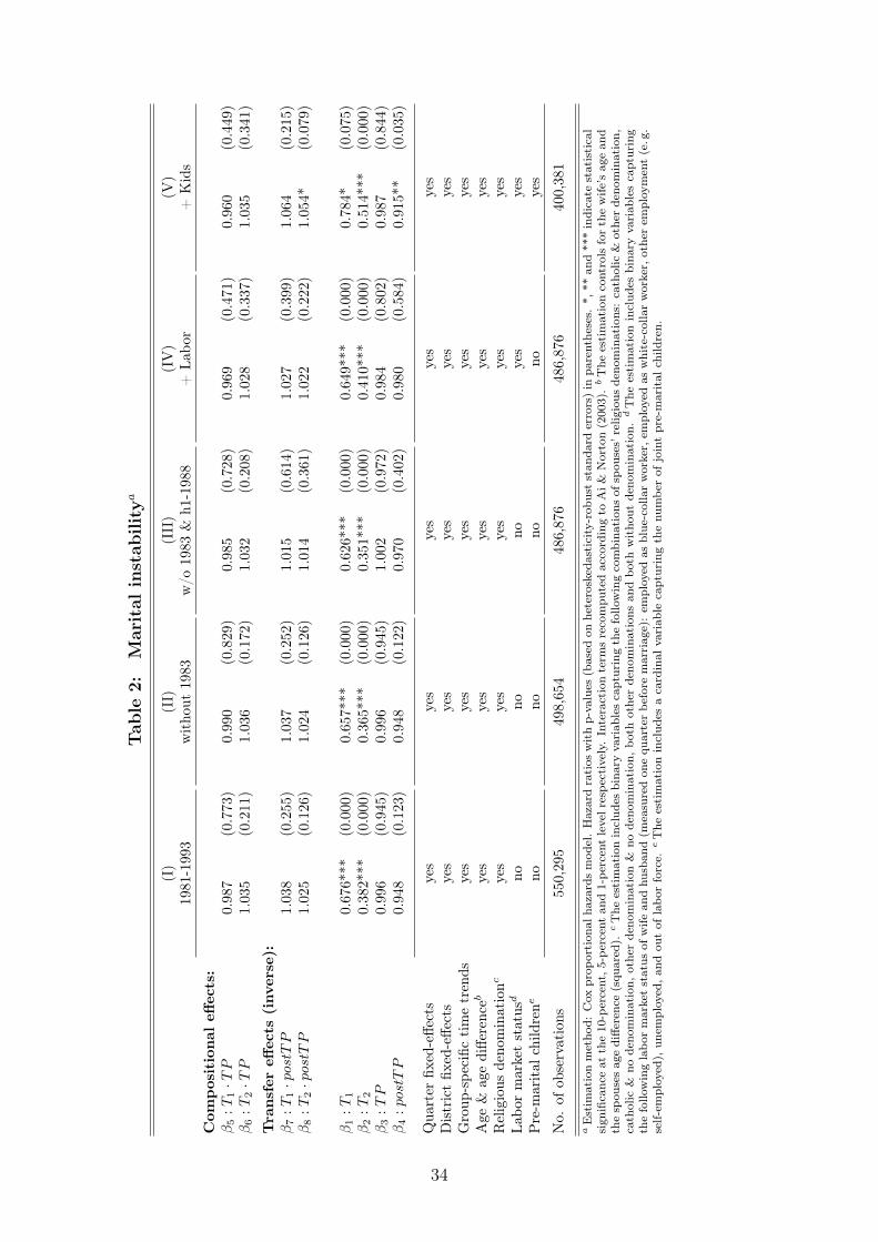
Tab

le2:

Mar

ital

inst

abilitya

(I)

(II)

(III

)(I

V)

(V)

1981

-199

3w

itho

ut19

83w

/o19

83&

h1-1

988

+La

bor

+K

ids

Com

positionaleffects:

�

5:T

1·T

P0.987

(0.773)

0.990

(0.829)

0.985

(0.728)

0.969

(0.471)

0.960

(0.449)

�

6:T

2·T

P1.035

(0.211)

1.036

(0.172)

1.032

(0.208)

1.028

(0.337)

1.035

(0.341)

Transfer

effects

(inverse):

�

7:T

1·p

ostTP

1.038

(0.255)

1.037

(0.252)

1.015

(0.614)

1.027

(0.399)

1.064

(0.215)

�

8:T

2·p

ostTP

1.025

(0.126)

1.024

(0.126)

1.014

(0.361)

1.022

(0.222)

1.054*

(0.079)

�

1:T

10.676*

**(0.000)

0.657*

**(0.000)

0.626*

**(0.000)

0.649*

**(0.000)

0.784*

(0.075)

�

2:T

20.382*

**(0.000)

0.365*

**(0.000)

0.351*

**(0.000)

0.410*

**(0.000)

0.514*

**(0.000)

�

3:TP

0.996

(0.945)

0.996

(0.945)

1.002

(0.972)

0.984

(0.802)

0.987

(0.844)

�

4:postTP

0.948

(0.123)

0.948

(0.122)

0.970

(0.402)

0.980

(0.584)

0.915*

*(0.035)

Qua

rter

fixed

-effe

cts

yes

yes

yes

yes

yes

Dis

tric

tfix

ed-e

ffect

sye

sye

sye

sye

sye

sG

roup

-spe

cific

tim

etr

ends

yes

yes

yes

yes

yes

Age

&ag

edi

ffere

nceb

yes

yes

yes

yes

yes

Rel

igio

usde

nom

inat

ionc

yes

yes

yes

yes

yes

Labo

rm

arke

tst

atus

dno

nono

yes

yes

Pre

-mar

ital

child

rene

nono

nono

yes

No.

ofob

serv

atio

ns55

0,29

549

8,65

448

6,87

648

6,87

640

0,38

1a

Est

imat

ion

met

hod:

Cox

prop

orti

onal

haza

rds

mod

el.

Haz

ard

rati

osw

ith

p-va

lues

(bas

edon

hete

rosk

edas

tici

ty-r

obus

tst

anda

rder

rors

)in

pare

nthe

ses.

*,**

and

***

indi

cate

stat

isti

cal

sign

ifica

nce

atth

e10

-per

cent

,5-p

erce

ntan

d1-

perc

ent

leve

lres

pect

ivel

y.In

tera

ctio

nte

rms

reco

mpu

ted

acco

rdin

gto

Ai&

Nor

ton

(200

3).

bT

hees

tim

atio

nco

ntro

lsfo

rth

ew

ife’s

age

and

the

spou

ses

age

diffe

renc

e(s

quar

ed).

cT

hees

tim

atio

nin

clud

esbi

nary

vari

able

sca

ptur

ing

the

follo

win

gco

mbi

nati

ons

ofsp

ouse

s’re

ligio

usde

nom

inat

ions

:ca

thol

ic&

othe

rde

nom

inat

ion,

cath

olic

&no

deno

min

atio

n,ot

her

deno

min

atio

n&

node

nom

inat

ion,

both

othe

rde

nom

inat

ions

and

both

wit

hout

deno

min

atio

n.d

The

esti

mat

ion

incl

udes

bina

ryva

riab

les

capt

urin

gth

efo

llow

ing

labo

rm

arke

tst

atus

ofw

ifean

dhu

sban

d(m

easu

red

one

quar

ter

befo

rem

arri

age)

:em

ploy

edas

blue

-col

lar

wor

ker,

empl

oyed

asw

hite

-col

lar

wor

ker,

othe

rem

ploy

men

t(e

.g.

self-

empl

oyed

),un

empl

oyed

,and

out

ofla

bor

forc

e.eT

hees

tim

atio

nin

clud

esa

card

inal

vari

able

capt

urin

gth

enu

mbe

rof

join

tpr

e-m

arit

alch

ildre

n.

34

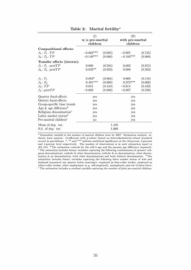
Table 3: Marital fertilitya

(I) (II)w/o pre-marital with pre-marital

children children

Compositional effects:

�5 : T1 · TP �0.062*** (0.005) �0.007 (0.745)�6 : T2 · TP �0.149*** (0.000) �0.103*** (0.000)

Transfer effects (inverse):

�7 : T1 · postTP 0.009 (0.594) 0.002 (0.915)�8 : T2 · postTP 0.032** (0.023) 0.008 (0.563)

�1 : T1 0.083* (0.064) 0.069 (0.118)�2 : T2 0.401*** (0.000) 0.373*** (0.000)�3 : TP 0.015 (0.410) �0.014 (0.433)�4 : postTP �0.003 (0.808) �0.007 (0.550)

Quarter fixed-effects yes yesDistrict fixed-effects yes yesGroup-specific time trends yes yesAge & age differenceb yes yesReligious denominationc yes yesLabor market statusd yes yesPre-marital childrene no yesMean of dep. var. 1.195S.d. of dep. var. 1.060a Dependent variable is the number of marital children born by 2007. Estimation method: or-dinary least squares. Coefficients with p-values (based on heteroskedasticity-robust standarderrors) in parentheses. *, ** and *** indicate statistical significance at the 10-percent, 5-percentand 1-percent level respectively. The number of observations is in each estimation equal to401, 314. b The estimation controls for the wife’s age and the spouses age difference (squared).c The estimation includes binary variables capturing the following combinations of spouses’ reli-gious denominations: catholic & other denomination, catholic & no denomination, other denom-ination & no denomination, both other denominations and both without denomination. d Theestimation includes binary variables capturing the following labor market status of wife andhusband (measured one quarter before marriage): employed as blue-collar worker, employed aswhite-collar worker, other employment (e. g. self-employed), unemployed, and out of labor force.e The estimation includes a cardinal variable capturing the number of joint pre-marital children.

35

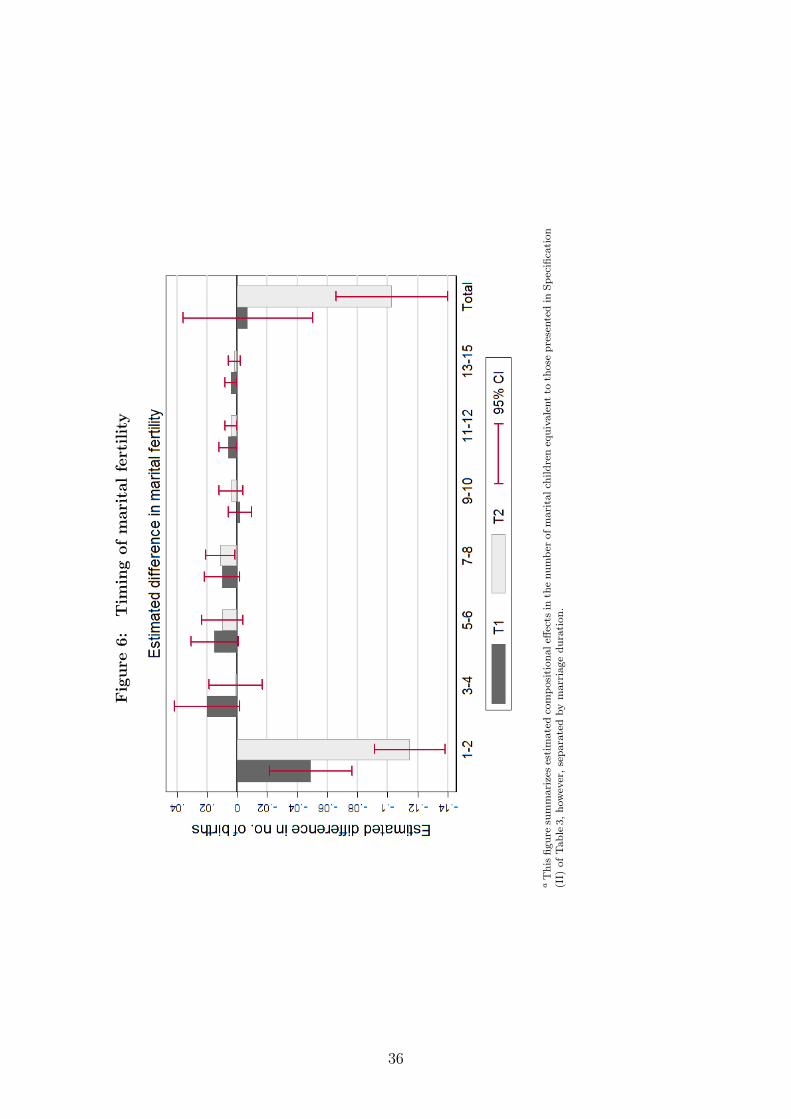
Fig

ure

6:T

imin

gof

mar

ital

fert

ility

aT

hisfig

ure

sum

mar

izes

esti

mat

edco

mpo

siti

onal

effec

tsin

the

num

berof

mar

ital

child

ren

equi

vale

ntto

thos

epr

esen

ted

inSp

ecifi

cati

on(I

I)of

Tab

le3,

how

ever

,sep

arat

edby

mar

riag

edu

rati

on.

36

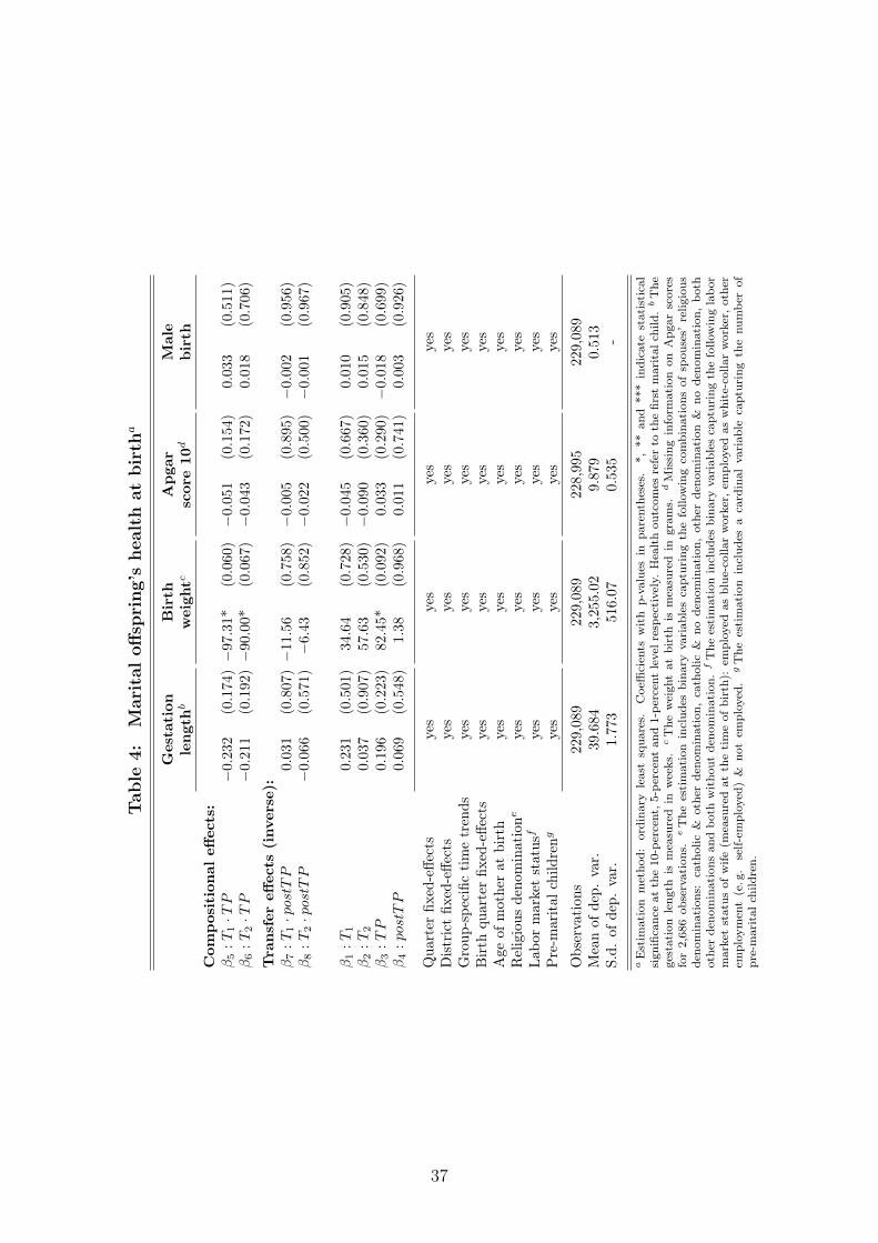
Tab

le4:

Mar

ital

offsp

ring’

shea

lth

atbir

tha

Gestation

Birth

Apgar

Male

length

bw

eight

cscore

10

dbirth

Com

positionaleffects:

�

5:T

1·T

P�0.232

(0.174)

�97

.31

*(0.060)

�0.051

(0.154)

0.033

(0.511)

�

6:T

2·T

P�0.211

(0.192)

�90

.00

*(0.067)

�0.043

(0.172)

0.018

(0.706)

Transfer

effects

(inverse):

�

7:T

1·p

ostTP

0.031

(0.807)

�11

.56

(0.758)

�0.005

(0.895)

�0.002

(0.956)

�

8:T

2·p

ostTP

�0.066

(0.571)

�6.43

(0.852)

�0.022

(0.500)

�0.001

(0.967)

�

1:T

10.231

(0.501)

34.64

(0.728)

�0.045

(0.667)

0.010

(0.905)

�

2:T

20.037

(0.907)

57.63

(0.530)

�0.090

(0.360)

0.015

(0.848)

�

3:TP

0.196

(0.223)

82.45

*(0.092)

0.033

(0.290)

�0.018

(0.699)

�

4:postTP

0.069

(0.548)

1.38

(0.968)

0.011

(0.741)

0.003

(0.926)

Qua

rter

fixed

-effe

cts

yes

yes

yes

yes

Dis

tric

tfix

ed-e

ffect

sye

sye

sye

sye

sG

roup

-spe

cific

tim

etr

ends

yes

yes

yes

yes

Bir

thqu

arte

rfix

ed-e

ffect

sye

sye

sye

sye

sA

geof

mot

her

atbi

rth

yes

yes

yes

yes

Rel

igio

usde

nom

inat

ione

yes

yes

yes

yes

Labo

rm

arke

tst

atus

fye

sye

sye

sye

sP

re-m

arital

child

reng

yes

yes

yes

yes

Obs

erva

tion

s22

9,08

922

9,08

922

8,99

522

9,08

9M

ean

ofde

p.va

r.39

.684

3,25

5.02

9.87

90.

513

S.d.

ofde

p.va

r.1.

773

516.

070.

535

-a

Est

imat

ion

met

hod:

ordi

nary

leas

tsq

uare

s.C

oeffi

cien

tsw

ith

p-va

lues

inpa

rent

hese

s.*,

**an

d**

*in

dica

test

atis

tica

lsi

gnifi

canc

eat

the

10-p

erce

nt,5

-per

cent

and

1-pe

rcen

tle

velr

espe

ctiv

ely.

Hea

lth

outc

omes

refe

rto

the

first

mar

ital

child

.bT

hege

stat

ion

leng

this

mea

sure

din

wee

ks.

cT

hew

eigh

tat

birt

his

mea

sure

din

gram

s.d

Mis

sing

info

rmat

ion

onA

pgar

scor

esfo

r2,

686

obse

rvat

ions

.eT

hees

tim

atio

nin

clud

esbi

nary

vari

able

sca

ptur

ing

the

follo

win

gco

mbi

nati

ons

ofsp

ouse

s’re

ligio

usde

nom

inat

ions

:ca

thol

ic&

othe

rde

nom

inat

ion,

cath

olic

&no

deno

min

atio

n,ot

her

deno

min

atio

n&

node

nom

inat

ion,

both

othe

rde

nom

inat

ions

and

both

wit

hout

deno

min

atio

n.f

The

estim

atio

nin

clud

esbi

nary

vari

able

sca

ptur

ing

the

follo

win

gla

bor

mar

ket

stat

usof

wife

(mea

sure

dat

the

tim

eof

birt

h):

empl

oyed

asbl

ue-c

olla

rw

orke

r,em

ploy

edas

whi

te-c

olla

rw

orke

r,ot

her

empl

oym

ent

(e.g

.se

lf-em

ploy

ed)

&no

tem

ploy

ed.

gT

hees

tim

atio

nin

clud

esa

card

inal

vari

able

capt

urin

gth

enu

mbe

rof

pre-

mar

ital

child

ren.

37