CAN Bus Experiments of Real-TimeCommunications

Fernando G. Tinetti?, Fernando L. Romero, Alejandro D. Perez

Instituto de Investigacion en Informatica LIDI (III-LIDI)Facultad de Informatica, UNLP, 50 y 120, La Plata, Argentina

{fernando, fromero}@lidi.info.unlp.edu.ar, perez.alejandrodaniel@gmail.com

Abstract. This paper presents a benchmark development and the anal-ysis of communication times in a CAN (Controller Area Network) bus.Preemptive and fixed priority scheduling is taken as departure point forthe initial experiments and analysis. This method would be adapted forprogramming CAN messages without preemption of the shared com-munications channel. It is also complemented by a specific priority as-signment algorithm, suitable for non-preemptive systems. A real CANnetwork is used for the experiments, and results are analyzed from thepoint of view of real-time performance and CAN specification. We havefound well known, deterministic, and correct performance communica-tion times. Messages and signals are delivered within deadlines, a funda-mental requirement for a real-time system.

Keywords: CAN Bus Implementation, Real-Time Experiments, Instru-mentation and Monitoring, Real-Time Schedulability

1 Introduction

The initial development of a CAN time analysis is based on [6], which defines apreemptive and fixed priority task scheduling (mainly) for single-processor sys-tems. This method is adapted for the programming of CAN messages and sev-eral enhancements defined in [2]. Basically, an optimal prioritization algorithmintroduced in [1] is applicable to non-proprietary systems. Enhancements andoptimizations can be experimentally verified (at least in part) by building a realCAN network where specific communication time measurements can be made.Time measurements/sampling can be then used for evaluating the fulfillment ofCAN real time requirements.

A CAN bus is arbitrated using priorities, and once the bus access is obtained,the message is transmitted in full. Thus, the bus appropriative policy preventsanother message from gaining access to the bus while a message is being trans-mitted. The priority inversion problem allowed by the CAN apropriativenessshould be addressed. Regardless of priority inversion, every message has its own

? Comision de Investigaciones Cientıficas, Prov. de Bs. As., corresponding author

deadline, and the bus arbitration will impose some delay that should be mini-mized in order to avoid real-time deadline violations. This work will be focusedon the behavior of the Data Frames transmission of the CAN standard.

Messages in the CAN bus are handled by controllers, and a single controllermay handle several CAN nodes. Also, each controller implements the bus arbi-tration while it maintains a queue of pending messages. The controller queue ismanaged according to fixed priority and non-preemptive scheduling. Controllersare synchronized at the start of a message with the clock of the sending node(rising edge). A transmission is allowed to start after the bus is idle for a 3-bit(interframe) period. A controller begins to transmit with a dominant bit (“’0”),which causes the rest of the controllers to synchronize with the rising edge ofthis bit and become receivers. Any message that is ready to be transmitted mustwait for another arbitration cycle to start when the bus is again idle. The CANprotocol requires the transmitter to insert a bit with opposite polarity every 5bits of the same polarity, a technique known as “bit stuffing”. Thus, a stuffingbit may be added every 4 bits of the message. Taking into account the messagebit length, mbl, the constant number of bits k needed for the node identification,the maximum number of bits added for stuffing, and the bit transmission time,τbit, the maximum transmission time of the message would be given by Mtm in(1).

Mtm =

(mbl + k +

⌊mbl + k − 1

4

⌋)τbit (1)

2 Waiting, Errors, and Maximum Time

Given a specific application or experiment, the message types are predefined,i.e. each message m has a unique and fixed identifier and priority. Messages arequeued in controllers by a software routine. Message queueing needs a run timebetween 0 and Jm, known as queuing the message jitter, and is inherited fromthe response time of the task, including the delay by polling [6]. The messagetime period Tm is considered for events that trigger the message queueing. Thereare three types of events associated with Tm: a) Events with exact period Tm,b) Events that occur sporadically with a minimum separation time Tm, and c)Events that occur only when the system starts. Each message has a hard deadlineDm, the maximum time from the initial event that generates the message to bequeued to the actual message arrival at destination.

The worst case for response time Rm of a message can be defined as thelongest time since the start event occurs until the message begins to be receivedby the node/s that require it. A message can be called “schedulable” if and onlyif its worst case response time is less than or equal to Dm: Rm ≤ Dm. The wholesystem is “schedulable” if and only if all the messages are schedulable. Rm isbasically the aggregation of: 1) The delay time Wm (also called Window time),which is the longest message waiting time in the CAN controller, and 2) Theworst message transmission time, Mtm. In turn, Wm is a function of: 1) Blockingtime, Bm, given by messages of lower priority in the transmission process, and

2) Interference time, where a message with higher priority is transmitted earlierthan m. The message blocking time can be calculated as Bm = max(Ck) withk ∈ lp(m), and lp(m) is the set of messages with lower priority than m. Theinterference time is closely related to the concept of “busy period” introducedin [5], where a busy period of level i is defined as the time interval [a, b] withinwhich the tasks with priority i or greater are processed within this interval andthere are no tasks with priority i in the intervals (a − t, a) and (b, b + t) witht > 0. Adapting this definition to the CAN protocol, we have a busy period ofpriority m. The period starts at a time Ts where a message of priority m orgreater is queued to transmit, and there are no queued messages of priority mor greater than m. It is a continuous interval of time, during which any prioritymessage less than m is not transmitted. Finally, the period ends at time Te,when the bus becomes ready for the next transmission and arbitration cycle andthere are no messages with priority greater than m.

The key characteristic of the busy period is that all messages of priority mor higher are transmitted within the period. In mathematical terms, the busyperiods can be seen as intervals [Ts, Te). Furthermore, the end of a busy periodmay coincide with the beginning of another busy period [5]. The busy periodelapsed time can be calculated as the maximum of tn+1

m given in equation 2,where gep(m) is the set of messages with priority greater than or equal to m,and f(tnm, tj) is the function that combines tnm with the times related to messagej: Jj (jitter) and Tj (time period).

tn+1m = Bm +

∑j∈gep(m)

⌈f(tnm, trj

⌉Cj (2)

The busy period time given by the recurrence in equation 2 monotonically growsfrom Bm up to one of the following values: a) tnm +Cm > Dm, which makes themessage non-schedulable or unschedulable, or b) tn+1

m = tnm, where the worstresponse time of the first instance of the message is reached in the busy perioddetermined by tnm + Cm

Errors and their related recovery times have to be taken into account whendealing with noisy environments. Each controller detecting an error starts arecovery process by transmitting an error signal. The resynchronization processtakes at least 29 bit transmission times. Furthermore, resynchronization is onlythe first step of the error recovery process. Other tasks (and their correspondingtimes) involved in the recovery process are those required to the retransmission ofthe message affected by errors. The equation including errors and their associatedtimes in noisy environments is given in equation 3, where Em involves at least the29-bit resynchronization and message retransmission, which is usually consideredin the analysis as the worst case overhead time as given in equation 4.

tm = Bm + Em +∑

j∈gep(m)

⌈f(tnm, trj

⌉Cj (3)

Overm = maxj∈gep(m)

(Cj) + 29τbit (4)

There are other details (and their corresponding times) involved in dealing witherrors, but the current work is focused on the basic analysis of CAN bus messagesand delay times. Thus, we will focus on a real CAN network and experimentationin the next section without taking into account errors and error recovery time/s.

3 Specific Benchmark

The Society of Automotive Engineers (SAE) provides a set of test data to eval-uate communication technologies handling the seven different subsystems in anelectric car prototype [6]. Signal data details are used to show a case of “real”use for the timing model of the previous section, with the 53 signals given bythe SAE and explained in [4]. The seven subsystems that generate signals in-clude the brakes, the driver himself, the engine, etc. In total there are 53 signals,characterized not only by the subsystem that generates them but by other im-portant details, such as the amount of information bits, if they are periodicor sporadic, jitter, etc. Every signal implies handling a message with specificreal-time latency/deadline.

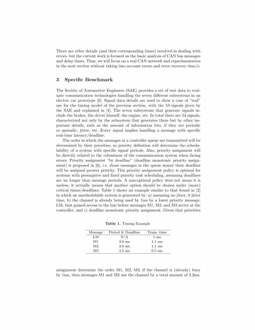
The order in which the messages in a controller queue are transmitted will bedetermined by their priorities, so priority definition will determine the schedu-lability of a system with specific signal periods. Also, priority assignment willbe directly related to the robustness of the communication system when facingerrors. Priority assignment “by deadline” (deadline monotonic priority assign-ment) is proposed in [6], i.e. those messages in the queue nearer their deadlinewill be assigned greater priority. This priority assignment policy is optimal forsystems with preemptive and fixed priority task scheduling, assuming deadlinesare no longer than message periods. A non-optimal policy does not mean it isuseless, it actually means that another option should be chosen under (more)critical times/deadlines. Table 1 shows an example similar to that found in [2]in which an unschedulable system is generated by: a) assuming no jitter, 0 jittertime, b) the channel is already being used by 1ms by a lower priority message,LM, that gained access to the bus before messages M1, M2, and M3 arrive at thecontroller, and c) deadline monotonic priority assignment. Given that priorities

Table 1. Timing Example

Message Period & Deadline Trans. time

LM N/A 1 msM1 3.0 ms 1.1 msM2 4.0 ms 1.1 msM3 4.5 ms 0.5 ms

assignment determine the order M1, M2, M3, if the channel is (already) busyby 1ms, then messages M1 and M2 use the channel by a total amount of 2.2ms.

Thus, while message M2 is being transmitted, a new instance of message M1,is queued and this new instance is the one with highest priority. Then, whilethe new instance of message M1 is being transmitted a new instance of messageM2 is queued, and message M3 is delayed beyond its deadline. The sequence ofmessages in the channel would be

LM => M1, after 1ms => M2, after 2.1ms => M1’, after 3.2msbecause the channel is not initially preempted from the lower priority message/s(represented by LM in the sequence above) and priorities are fixed and deter-mined by deadline/s. However, if the order of messages is determined as M1, M3,and M2 the worst response times are RM1 = 2.1ms, RM2 = 2.6ms, and RM3

= 3.7ms. Thus, this new priority assignment determines a schedulable system,where response times Rm < Dm, ∀m. The new priority assignment imply thefollowing sequence of messages in the communication channel

LM => M1, after 1ms => M3, after 2.1ms => M2, after 2.6msand no new instances of messages M1 and M2 will generate any delay on messageM3. In this context, the priority assignment algorithm given in [1] is claimed tobe optimal in non-preemptive systems in [3]. In general, the algorithm given in[1] is useful as long as the worst case of response time of a message: a) does notdepend on an ordering of the highest priority messages, and b) does not changeits length (it is not made longer, in particular) when having a higher priority.

The length of the delay queue and the length of the busy period do not dependon a specific order of the high priority messages. The blocking time, Bm, can bemade longer by changing the priority, but at the same time the interference isdecreased. The priority assignment algorithm given in [1] performs a maximumof n(n − 1)/2 evaluations for n messages, and guarantees message schedulingwhen possible. It should be borne in mind that the algorithm does not specifyan order in which messages should be analyzed at each priority level. This ordergreatly influences the priority assignment if there is more than one scheduling,and a poor choice of initial order may result in a non-optimal scheduling.

Given a set of CAN messages, it is possible to assign the correspondingpriorities by following a sequence of simple steps

1. Define the message characteristics: size, identifier, bus speed, etc.2. Sort messages by some criterion, whether those given in [6] or [1].3. Apply the timing model to each message. Usually, it is possible to analyze

the minimum transmission rate at which the system is schedulable.

In the case of the SAE signals and data, the “D - J” method given in [6] will beused as a guide, in which higher priority is assigned to signals with lower waitingtime, (that is, a smaller D - J value, being D and J Deadline time and Waitingtime, respectively). Once signals have their priorities, it is possible to analizethe system’s schedulability with the timing model given above and consideringthe data rate of the communication channel. Besides, the channel utilization ismay be enhanced with a technique referred to as “piggyback”. Basically, thepiggyback technique takes advantage of periodic signals that can be grouped ina single message. Table 2 shows the first 10 signals defined by the SAE, all ofthem of a single-byte periodic signals with deadline time (D) equal to period

(P), and jitter time given as J, where it is possible to identify 4 signals withthe same period from the same source. More specifically, signals 1, 2, 4, and 6from the Battery subsystem are sent every 100 ms. Instead of sending 4 one-bytemessages, a single message is sent with 4 bytes using the piggyback technique.Piggybacking reduces bus overhead of three messages. The transmission of adata byte can require the transmission of up to 63 bits. This technique can beextended to periodic signals that have different periods, as long as the minimumtime period is a divisor of the other period times. For example, signals 29, 30,and 32 have the same source subsystem, with periods 10 ms, 10 ms, and 5 msrespectively. Thus, every 2 messages of signal 32, the signals 29 and 30 can beadded to the same message with piggybacking.

Table 2. First 10 SAE Signals

#S Signal From D = P J

1 Hi&Lo Contactor Open/Close Battery 100 ms 0.6 ms2 Brake Pressure, Line Battery 100 ms 0.7 ms3 Processed Motor Speed Battery 1000 ms 1.0 ms4 Torque Command Battery 100 ms 0.8 ms5 Brake Pressure, Master Cylinder Battery 1000 ms 1.1 ms6 Accelerator Position Battery 100 ms 0.9 ms7 Torque Measured Driver 5 ms 0.1 ms8 Transaction Clutch Line Pressure Brakes 5 ms 0.1 ms9 Clutch Pressure Control Brakes 5 ms 0.2 ms10 High Contactor Control Trans 100 ms 0.2 ms

The piggyback technique can also be applied to sporadic signals. These sig-nals can be sent in a “server” message where the station sending the messagechecks for the occurrence of the sporadic signal before queuing the message.With this approach, a sporadic signal can be delayed no longer than the pollingperiod time, plus the worst latency time of the “server” message. For a messagewith deadline of 20 ms, a server message with a 15 ms polling period and 5 msworst case latency the technique would be good enough. Combining piggyback-ing with “server” messages for the sporadic signals the SAE benchmark/systemis schedulable with a data rate of 125 Kb/s. Piggybacking provides most of theoptimization, making possible channel utilization below 100%.

4 Experiments on a Real CAN Network

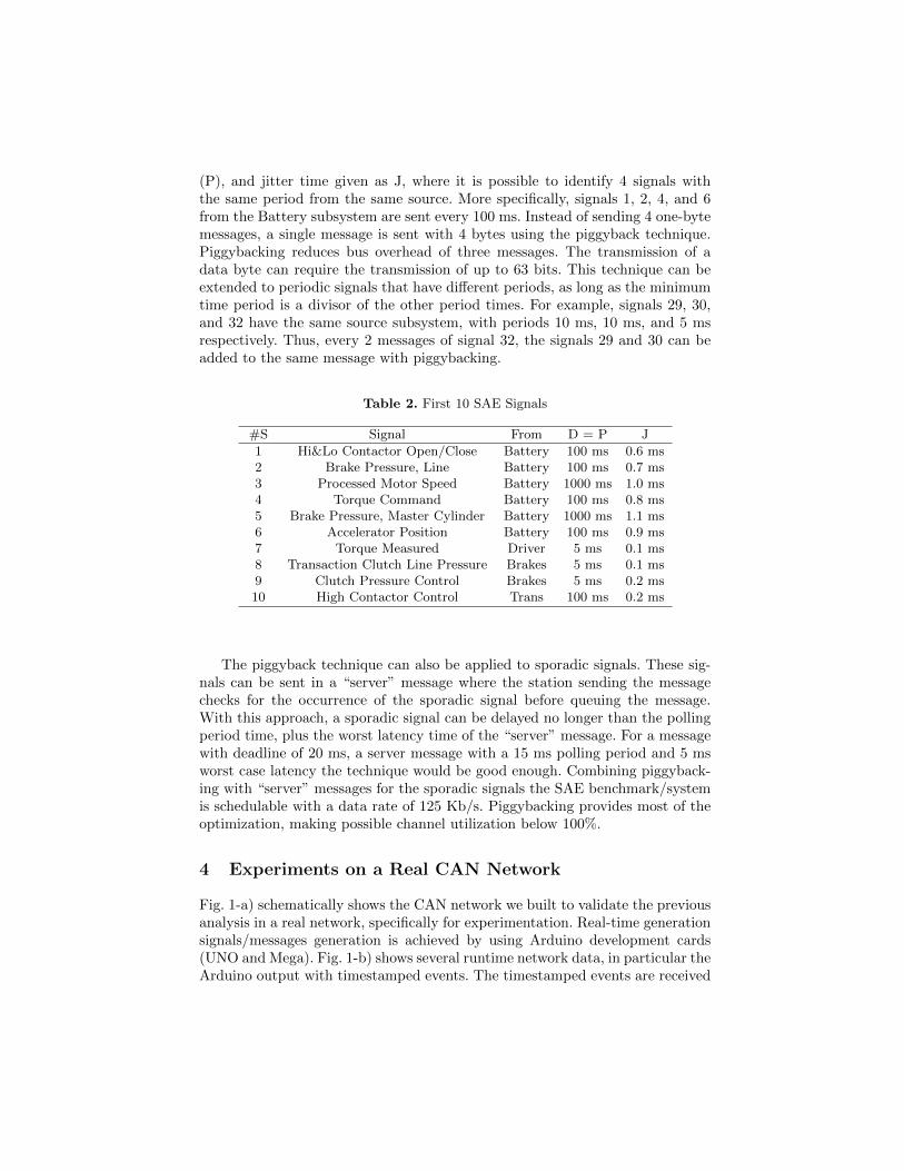
Fig. 1-a) schematically shows the CAN network we built to validate the previousanalysis in a real network, specifically for experimentation. Real-time generationsignals/messages generation is achieved by using Arduino development cards(UNO and Mega). Fig. 1-b) shows several runtime network data, in particular theArduino output with timestamped events. The timestamped events are received

in the PC at runtime from the Arduino Mega. Data shown on the screen is onlyfor visual monitoring, the real-time and precise timing calculations are made ina spreadsheet after each specific experiment.

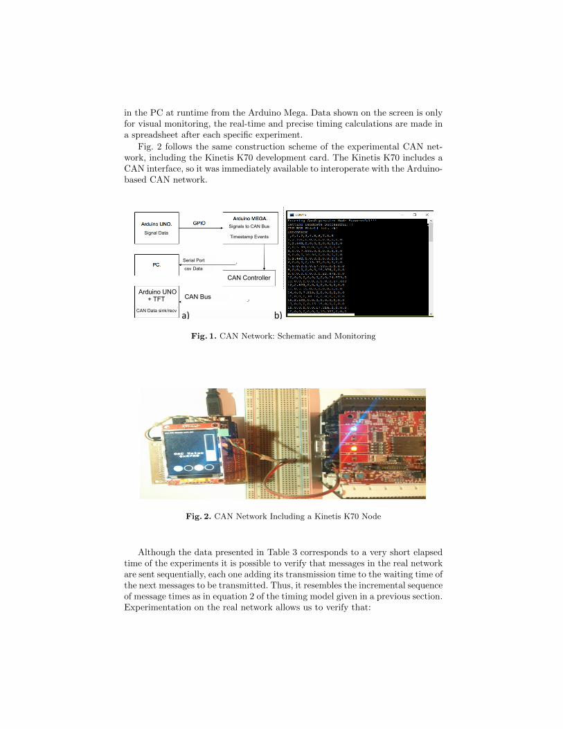
Fig. 2 follows the same construction scheme of the experimental CAN net-work, including the Kinetis K70 development card. The Kinetis K70 includes aCAN interface, so it was immediately available to interoperate with the Arduino-based CAN network.

a) b)

Signal Data

Signals to CAN Bus

Timestamp Events

CAN Controller

Arduino UNO + TFT

CAN Data sink/recv

Serial Port

csv Data

CAN Bus

Fig. 1. CAN Network: Schematic and Monitoring

Fig. 2. CAN Network Including a Kinetis K70 Node

Although the data presented in Table 3 corresponds to a very short elapsedtime of the experiments it is possible to verify that messages in the real networkare sent sequentially, each one adding its transmission time to the waiting time ofthe next messages to be transmitted. Thus, it resembles the incremental sequenceof message times as in equation 2 of the timing model given in a previous section.Experimentation on the real network allows us to verify that:

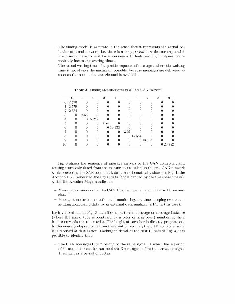
– The timing model is accurate in the sense that it represents the actual be-havior of a real network, i.e. there is a busy period in which messages withlow priority have to wait for a message with high priority, implying mono-tonically increasing waiting times.

– The actual writing time of a specific sequence of messages, where the waitingtime is not always the maximum possible, because messages are delivered assoon as the communication channel is available.

Table 3. Timing Measurements in a Real CAN Network

0 1 2 3 4 5 6 7 8 9

0 2.576 0 0 0 0 0 0 0 0 01 2.579 0 0 0 0 0 0 0 0 02 2.584 0 0 0 0 0 0 0 0 03 0 2.66 0 0 0 0 0 0 0 04 0 0 5.248 0 0 0 0 0 0 05 0 0 0 7.84 0 0 0 0 0 06 0 0 0 0 10.432 0 0 0 0 07 0 0 0 0 0 13.27 0 0 0 08 0 0 0 0 0 0 15.564 0 0 09 0 0 0 0 0 0 0 18.163 0 0

10 0 0 0 0 0 0 0 0 0 20.752

Fig. 3 shows the sequence of message arrivals to the CAN controller, andwaiting times calculated from the measurements taken in the real CAN networkwhile processing the SAE benchmark data. As schematically shown in Fig. 1, theArduino UNO generated the signal data (those defined by the SAE benchmark),which the Arduino Mega handles for

– Message transmission to the CAN Bus, i.e. queueing and the real transmis-sion.

– Message time instrumentation and monitoring, i.e. timestamping events andsending monitoring data to an external data analizer (a PC in this case).

Each vertical bar in Fig. 3 identifies a particular message or message instance(where the signal type is identified by a color or gray level) numbering themfrom 0 onwards (on the x-axis). The height of each bar is directly proportionalto the message elapsed time from the event of reaching the CAN controller untilit is received at destination. Looking in detail at the first 10 bars of Fig. 3, it ispossible to identify that:

– The CAN messages 0 to 2 belong to the same signal, 0, which has a periodof 30 ms, so the sender can send the 3 messages before the arrival of signal1, which has a period of 100ms.

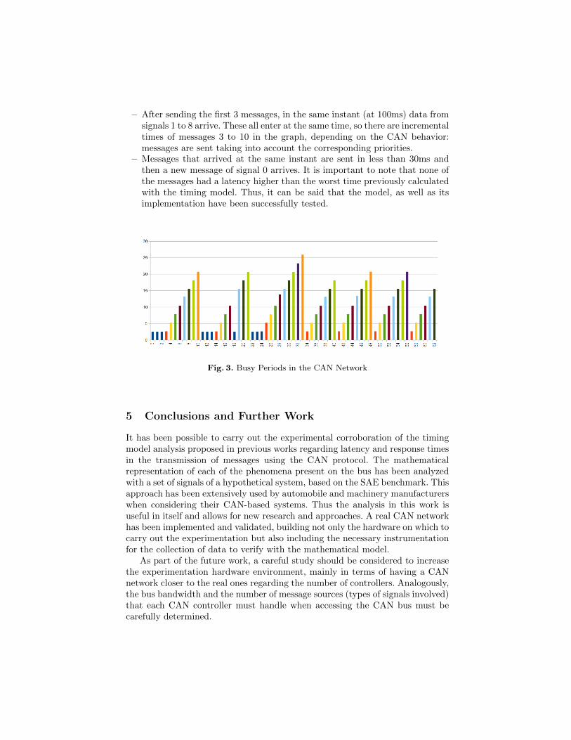
– After sending the first 3 messages, in the same instant (at 100ms) data fromsignals 1 to 8 arrive. These all enter at the same time, so there are incrementaltimes of messages 3 to 10 in the graph, depending on the CAN behavior:messages are sent taking into account the corresponding priorities.

– Messages that arrived at the same instant are sent in less than 30ms andthen a new message of signal 0 arrives. It is important to note that none ofthe messages had a latency higher than the worst time previously calculatedwith the timing model. Thus, it can be said that the model, as well as itsimplementation have been successfully tested.

Fig. 3. Busy Periods in the CAN Network

5 Conclusions and Further Work

It has been possible to carry out the experimental corroboration of the timingmodel analysis proposed in previous works regarding latency and response timesin the transmission of messages using the CAN protocol. The mathematicalrepresentation of each of the phenomena present on the bus has been analyzedwith a set of signals of a hypothetical system, based on the SAE benchmark. Thisapproach has been extensively used by automobile and machinery manufacturerswhen considering their CAN-based systems. Thus the analysis in this work isuseful in itself and allows for new research and approaches. A real CAN networkhas been implemented and validated, building not only the hardware on which tocarry out the experimentation but also including the necessary instrumentationfor the collection of data to verify with the mathematical model.

As part of the future work, a careful study should be considered to increasethe experimentation hardware environment, mainly in terms of having a CANnetwork closer to the real ones regarding the number of controllers. Analogously,the bus bandwidth and the number of message sources (types of signals involved)that each CAN controller must handle when accessing the CAN bus must becarefully determined.

References

1. Audsley, N.: Optimal priority assignment and feasibility of static priority tasks witharbitrary start times (1991)

2. Davis, R.I., Burns, A., Bril, R.J., Lukkien, J.J.: Controller area network (can)schedulability analysis: Refuted, revisited and revised. Real-Time Systems 35(3),239–272 (Apr 2007), https://doi.org/10.1007/s11241-007-9012-7

3. George, L., Rivierre, N., Spuri, M.: Preemptive and Non-Preemptive Real-Time UniProcessor Scheduling. Research Report RR-2966, INRIA (1996),https://hal.inria.fr/inria-00073732, projet REFLECS

4. Kopetz, H.: A solution to an automotive control system benchmark. In: 1994 Pro-ceedings Real-Time Systems Symposium. pp. 154–158 (Dec 1994)

5. Lehoczky, J.P.: Fixed priority scheduling of periodic task sets with arbitrary dead-lines. In: [1990] Proceedings 11th Real-Time Systems Symposium. pp. 201–209 (Dec1990)

6. Tindell, K., Burns, A., Wellings, A.: Calculating controller area network (can)message response times. Control Engineering Practice 3(8), 1163 – 1169 (1995),http://www.sciencedirect.com/science/article/pii/0967066195001128