CalPro: A Spreadsheet · CalPro: A Spreadsheet Program for the ... a spread-sheet program for the management of ... CalPro is an add-in program developed to work with Microsoft Excel

United StatesDepartment ofAgriculture

Forest Service

Pacific NorthwestResearch Station

General TechnicalReportPNW-GTR-619November 2004

CalPro: A SpreadsheetProgram for theManagement of CaliforniaMixed-Conifer StandsJingjing Liang, Joseph Buongiorno, and Robert A. Monserud

The Forest Service of the U.S. Department of Agriculture is dedicated to the principle ofmultiple use management of the Nation’s forest resources for sustained yields of wood,water, forage, wildlife, and recreation. Through forestry research, cooperation with theStates and private forest owners, and management of the National Forests and NationalGrasslands, it strives—as directed by Congress—to provide increasingly greater service toa growing Nation.

The U.S. Department of Agriculture (USDA) prohibits discrimination in all its programsand activities on the basis of race, color, national origin, gender, religion, age, disability,political beliefs, sexual orientation, or marital or family status. (Not all prohibited basesapply to all programs.) Persons with disabilities who require alternative means for commu-nication of program information (Braille, large print, audiotape, etc.) should contactUSDA’s TARGET Center at (202) 720-2600 (voice and TDD).

To file a complaint of discrimination, write USDA, Director, Office of Civil Rights, Room326-W, Whitten Building, 14th and Independence Avenue, SW, Washington, DC 20250-9410 or call (202) 720-5964 (voice and TDD). USDA is an equal opportunity provider andemployer.

USDA is committed to making the information materials accessible to all USDA customersand employees

AuthorsJingjing Liang is a research assistant and Joseph Buongiorno is the John N.

McGovern Professor, Department of Forest Ecology and Management, University

of Wisconsin-Madison, 1630 Linden Drive, Madison, WI 53706; and Robert A.

Monserud is a research forester, U.S. Department of Agriculture, Forest Service,

Pacific Northwest Research Station, 620 SW Main St., Suite 400, Portland, OR

97205.

Photo CreditCover photo by Jeremy Fried

AbstractLiang, Jingjing; Buongiorno, Joseph; Monserud, Robert A. 2004. CalPro: a spread-

sheet program for the management of California mixed-conifer stands. Gen. Tech.

Rep. PNW-GTR-619. Portland, OR: U.S. Department of Agriculture, Forest

Service, Pacific Northwest Research Station. 32 p.

CalPro is an add-in program developed to work with Microsoft Excel to simulate the

growth and management of uneven-aged mixed-conifer stands in California. Its built-in

growth model was calibrated from 177 uneven-aged plots on industry and other private

lands. Stands are described by the number of trees per acre in each of nineteen 2-inch

diameter classes in two species groups, hardwoods and softwoods.

CalPro allows managers to predict stand development by year and for many

decades from a specific initial state. Users can choose cutting regimes by specifying the

interval between harvests (cutting cycle) and a target distribution of trees remaining

after harvest. A target distribution can be a reverse-J-shaped distribution or any other

desired distribution. Diameter-limit cuts can also be simulated. Tabulated and graphic

results show diameter distributions, basal area, volumes, income, net present value, and

indices of stand diversity by species and size.

This manual documents the program installation and activation, provides sugges-

tions for working with Excel, and gives background information on CalPro’s growth

model. It offers a comprehensive tutorial in the form of two practical examples that

explain how to start the program, enter simulation data, execute a simulation, compare

simulations, and plot summary statistics.

Keywords: Mixed conifers, uneven-aged management, economics, ecology,

CalPro, simulation, software, growth model, diversity.

Contents1 1. Introduction1 What Is CalPro?1 Why Simulate This Type of Stand?2 How Does CalPro Work?2 What Is in This Manual?2 2. Getting Started2 System Requirements2 Installing CalPro4 Uninstalling CalPro4 3. Using CalPro4 CalPro Input5 BDq Calculator6 Storing Data and Retrieving Stored Data6 Running Simulations7 Quitting CalPro7 4. Examples7 Simulating the Lexen Stocking Standard

15 Simulating BDq and Diameter-Limit Management Regimes21 5. Troubleshooting CalPro22 Acknowledgments22 Metric Equivalents23 Literature Cited25 Appendix 1: CalPro Data27 Appendix 2: Growth-and-Yield Model30 Appendix 3: Definition of Diversity of Tree Species and Size31 Glossary

CalPro: A Spreadsheet Program for the Management of California Mixed-Conifer Stands

1

I. IntroductionWelcome to CalPro—a spreadsheet program to help with management decisions

using uneven-aged systems in mixed-conifer forests. This paper provides back-

ground, instruction, and additional suggestions for using the CalPro program. The

examples contain detailed instructions for each step. If you are new to CalPro, it

will be useful to run these examples while reading the paper.

What Is CalPro?

CalPro is a computer program meant to predict the development of mixed-conifer

stands in California. With this program, various management regimes can be

considered, and their outcomes can be quickly predicted. Three relatives of CalPro

(NorthPro, WestPro, and SouthPro) already exist for northern hardwoods in

Wisconsin and Michigan (Liang et al. 2004), for Douglas-fir (Pseudotsuga

menziesii (Mirb.) Franco) in the Pacific Northwest region of the United States

(Ralston et al. 2003), and for loblolly pine (Pinus taeda L.) in the Southern United

States (Schulte et al. 1998), respectively. We have used our experience with these

programs to further simplify the data input and the program output to maximize

CalPro’s usefulness for practitioners.

Why Simulate This Type of Stand?

Mixed-conifer forests compose one of the largest vegetation types in California,

covering 13 percent of the state’s area (Barbour and Major 1977). The expansive-

ness of the mixed-conifer types and the amount of timber harvested from the west

slopes of the Sierra Nevada Mountains emphasize the need for accurate growth-

and-yield prediction methods applicable to mixed-conifer stands. Uneven-aged

management, selecting single trees or small groups of trees at intervals of 5 to 20

years and encouraging natural regeneration, helps maintain a continuous tree cover

with aesthetic and ecological benefits (DeBell and Franklin 1987). Some of the

examples in this manual also suggest that effective uneven-aged management of

mixed conifers can be profitable. CalPro helps foresters predict how a given

forest stand might look in the future and what it could yield under uneven-aged

management.

GENERAL TECHNICAL REPORT PNW-GTR-619

2

How Does CalPro Work?

CalPro predictions are based on a multispecies, site- and density-dependent matrixgrowth model for California,1 an extension of earlier density-dependent matrixmodels (Lu and Buongiorno 1993). The data used to calibrate the growth modelcame from plots remeasured in two surveys in the 1980s and 1990s in forest standsin the Sierra Nevada Mountains (app. 1).

The equations built in CalPro predict growth, mortality, and the rate ofingrowth (recruitment) for hardwood and softwood species. The model equationsare in appendix 2.

What Is in This Manual?

The next section explains how to install CalPro on your computer and provides adescription of the input data, as well as instructions for loading and saving thesedata, running simulations, and saving the results. Two examples of applications aregiven. We included answers to some common questions. The manual assumes thatyou are familiar with the basics of Microsoft Excel.

2. Getting StartedSystem Requirements

You need the following hardware and software to operate CalPro:

• A computer (PC) with at least 16 megabytes of random access memory (RAM)• Windows® 95, 98, 2000, Me, XP, or Windows NT™ 4

2

• Microsoft Excel 5.0 to Excel 2002• A free copy of the CalPro software downloaded from

http://forest.wisc.edu/facstaff/buongiorno/index.htm or from the authorsthrough [email protected].

Installing CalPro

To install the program for the first time:

1. Insert the diskette containing CalPro.xla into your computer, or download itfrom the Web site to your local disk and go to step 3.

2. Select the CalPro.xla icon and copy it onto your hard disk. For your conven-ience, you may save it in a new folder named CalPro, e.g.,C:\CalPro\CalPro.xla.

1 Liang, J.J.; Buongiorno, J.; Monserud, R.A. Estimation and application of a growth and

yield model for uneven-aged mixed conifer stands in California. Forest Ecology andManagement. Manuscript in preparation. On file with: R. Monserud, Pacific NorthwestResearch Station, 620 SW Main St., Suite 400, Portland, OR 97205.2 The use of trade or firm names in this publication is for reader information and does not

imply endorsement by the U.S. Department of Agriculture of any product or service.


3

3. Open Microsoft Excel and START A NEW WORKBOOK.

4. Under the Tools menu, select Add-ins. In the add-ins dialogue box, select

Browse and choose CalPro.xla from its location on your hard disk. Click OK.

5. Return to the Tools menu and notice that CalPro is now the last choice in the

menu. Select CalPro and click OK in the title box.

6. The CalPro menu should now be in the Excel menu bar.

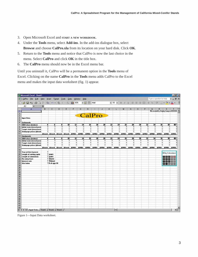
Until you uninstall it, CalPro will be a permanent option in the Tools menu of

Excel. Clicking on the name CalPro in the Tools menu adds CalPro to the Excel

menu and makes the input data worksheet (fig. 1) appear.

Figure 1—Input Data worksheet.


4

There are five sample workbooks at our Web site with the input data

worksheets corresponding to the examples in section 4 of this paper. By copying

the data from these worksheets into your input data worksheet you will be able to

run these examples with CalPro.

Uninstalling CalPro

To remove the CalPro menu and uninstall the program:

1. Close all Excel windows.

2. Select the file CalPro.xla and delete it from your hard disk.

3. Open Microsoft Excel and start a new workbook.

4. Under the Tools menu, select Add-ins. Deselect CalPro to remove the title

from the add-ins list.

5. Close the Excel window.

3. Using CalPro

CalPro Input

In the input data worksheet (fig. 1), each cell with a question mark requires a

numeric entry. CalPro automatically converts numeric entries to one or two deci-

mal places.

In figure 1, the two rows labeled “initial state” contain the initial number of

trees per acre in the stand (at time zero), by species groups and by 2-in diameter

classes. CalPro recognizes two species groups, hardwoods and softwoods (app. 1).

The two rows labeled “target state” contain the number of trees per acre, by

species group and by diameter class that should remain after harvest. A target entry

of zero instructs CalPro to harvest all trees in that species category and diameter

class. When the number of trees in the stand exceeds the target value, the harvest

is the difference between the available trees and the target; otherwise the harvest is

zero. You can always prevent the removal of any tree by entering a very high target,

e.g., 1,000.

The data in the rows labeled “Stumpage prices” are in dollars per cord (1 cord

= 128 ft3) for trees of pole size. They are in dollars per thousand board feet (MBF)

for trees of sawtimber size.

CalPro measures time in years. All simulations start at time zero and last for

the “Length of simulation.” The “Year of first harvest” may be set at any

nonnegative value. The “Length of cutting cycle,” i.e., the interval between


5

harvests, must be at least 1 year. To simulate stand growth without harvest, set the

“Year of first harvest” to a value greater than the “Length of simulation.”

The “Re-entry Cost” represents cost of doing a harvest, in dollars per acre,

independent of the volume harvested. The cost of timber sale preparation and

administration would be part of a typical re-entry cost.

The “Site Index” is measured by the average total height of the dominant and

codominant trees at 50 years of age (Hanson et al. 2002). The site index should be

between 30 and 99, the range of site-index values on the plots used to calibrate

CalPro.

CalPro treats empty input data cells as errors and will prompt you to fix them.

You can enter zeros for Stumpage prices, Re-entry Cost, and Interest rate if you

do not want a financial analysis.

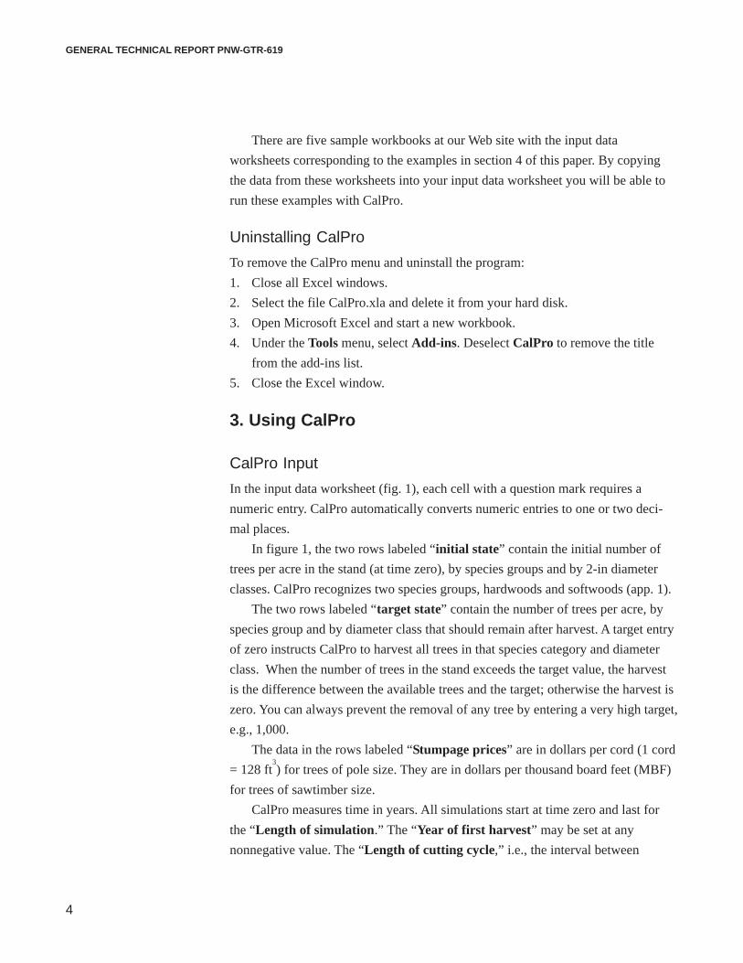
BDq Calculator

A BDq distribution is a tree distribution, by diameter class, defined by a stand basal

area (B), a maximum and minimum tree diameter (D), and a q-ratio (q), the ratio of

the number of trees in a given diameter class to the number of trees in the next

larger class. You can use the BDq calculator to define either the target state or the

initial state with a BDq distribution.

To use the BDq calculator, click on the BDq calculator icon in the input data

worksheet. Use the arrow buttons to set the stand basal area (ft2/ac), the q-ratio, the

minimum and the maximum diameters (in); click the Calculate button (fig. 2).

The example in figure 2 shows the number of trees by diameter class that

would give a basal area of 90 ft2/ac with trees of diameters from 3 to 40 in and a

q-ratio of 1.7. You can copy the resulting stand distribution to the input data

worksheet as the initial distribution or as the target distribution for a species group

by selecting the destination and clicking the Copy button on the BDq calculator

(fig. 2).

Figure 2—The BDq Distribution Calculator window.


6

Storing Data and Retrieving Stored Data

After entering data in the Input Data worksheet, you can save this worksheet for

later use. You should save your work frequently to avoid losing data. It is advisable

to save the work in a particular folder to facilitate locating the file in the future.

To run several simulations, e.g., to examine the effects of changing some of the

parameters, you may find it efficient to work with previously saved input data. To

retrieve the data, choose the File�Open command in Excel to open your saved file

or double click on the file icon.

Running Simulations

After completing the input data worksheet or retrieving a previously saved one, you

are ready to run a simulation. To run CalPro, make sure that the CalPro menu is in

the Excel menu bar. If not, click CalPro under the Tools menu to activate CalPro.

You can then run the simulation by choosing Run in the CalPro menu.

Each CalPro simulation generates the following worksheets and charts:• A TreesPerAcre worksheet: The number of trees by species and diameter

class for each simulated year.• A Basal Area worksheet: The basal area by species and diameter class, for

each simulated year.• A Products worksheet: The physical output and the financial return from the

harvests throughout the simulation.• A Diversity worksheet: Shannon’s species diversity indices and size diversity

indices for each year of the simulation.• A Diversity chart: A plot of Shannon’s indices of species and size diversity

over time.• A Species BA chart: A stacked area chart showing the development of stand

basal area by species group over time.• A Size BA chart: A stacked area chart showing the development of stand basal

area by timber size over time.

To compare various management regimes, save the output worksheets immediately

after running a simulation. Otherwise CalPro will overwrite the previous results

every time you run a new simulation.

All the data in the output worksheets are protected and you cannot change

them. To see how results change with different input data, change the input data

worksheet and rerun the simulation.


7

Quitting CalPro

To finish working with CalPro, choose the command Quit under the CalPro menu.

The CalPro menu will then disappear, but the current worksheets will stay in the

Excel window until you close them.

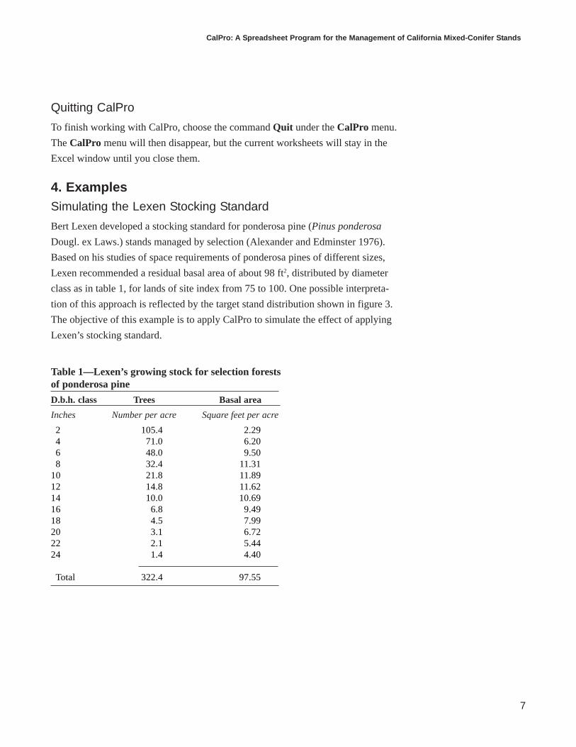
4. ExamplesSimulating the Lexen Stocking Standard

Bert Lexen developed a stocking standard for ponderosa pine (Pinus ponderosa

Dougl. ex Laws.) stands managed by selection (Alexander and Edminster 1976).

Based on his studies of space requirements of ponderosa pines of different sizes,

Lexen recommended a residual basal area of about 98 ft2, distributed by diameter

class as in table 1, for lands of site index from 75 to 100. One possible interpreta-

tion of this approach is reflected by the target stand distribution shown in figure 3.

The objective of this example is to apply CalPro to simulate the effect of applying

Lexen’s stocking standard.

Table 1—Lexen’s growing stock for selection forestsof ponderosa pine

D.b.h. class Trees Basal area

Inches Number per acre Square feet per acre

2 105.4 2.294 71.0 6.206 48.0 9.508 32.4 11.31

10 21.8 11.8912 14.8 11.6214 10.0 10.6916 6.8 9.4918 4.5 7.9920 3.1 6.7222 2.1 5.4424 1.4 4.40

Total 322.4 97.55


8

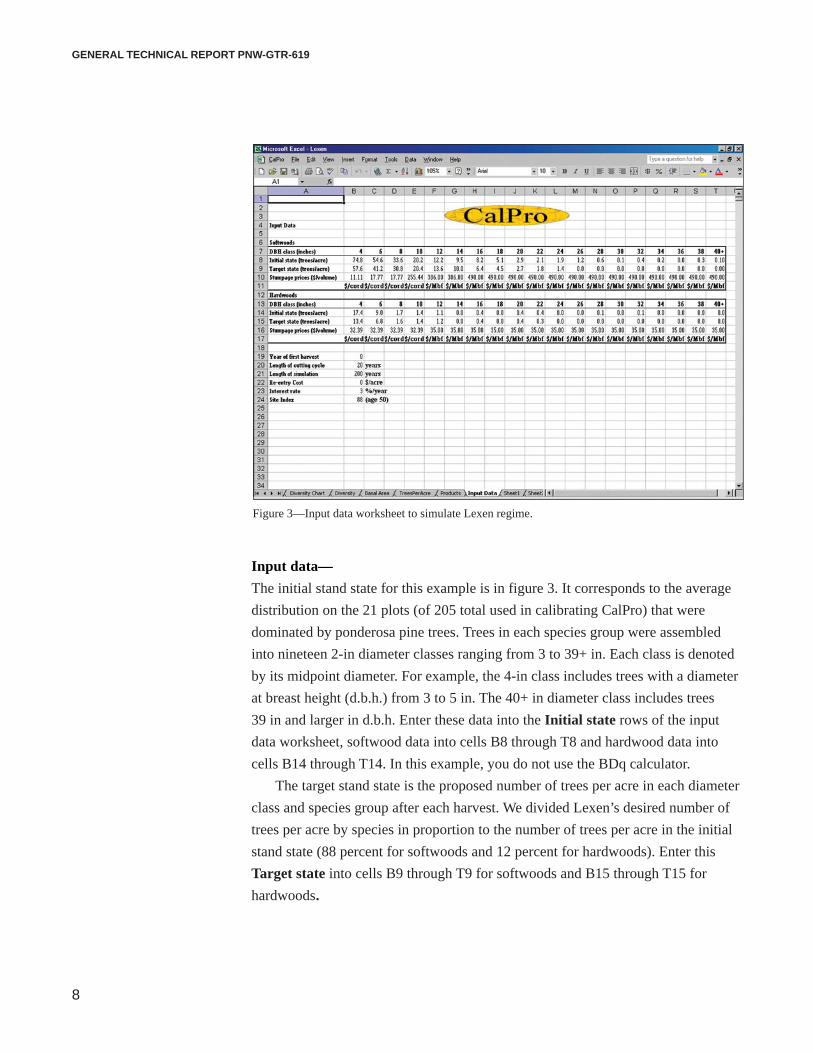
Input data—

The initial stand state for this example is in figure 3. It corresponds to the average

distribution on the 21 plots (of 205 total used in calibrating CalPro) that were

dominated by ponderosa pine trees. Trees in each species group were assembled

into nineteen 2-in diameter classes ranging from 3 to 39+ in. Each class is denoted

by its midpoint diameter. For example, the 4-in class includes trees with a diameter

at breast height (d.b.h.) from 3 to 5 in. The 40+ in diameter class includes trees

39 in and larger in d.b.h. Enter these data into the Initial state rows of the input

data worksheet, softwood data into cells B8 through T8 and hardwood data into

cells B14 through T14. In this example, you do not use the BDq calculator.

The target stand state is the proposed number of trees per acre in each diameter

class and species group after each harvest. We divided Lexen’s desired number of

trees per acre by species in proportion to the number of trees per acre in the initial

stand state (88 percent for softwoods and 12 percent for hardwoods). Enter this

Target state into cells B9 through T9 for softwoods and B15 through T15 for

hardwoods.

Figure 3—Input data worksheet to simulate Lexen regime.


9

Enter the Stumpage prices in cells B10 through T10 for softwoods and B16

through T16 for hardwoods. Enter the Re-entry Cost into cell B26, assumed to be

zero in the absence of timber sale preparation and administration.

Enter into cell B23 the real Interest rate of 3 percent per year, which is the

projected return on the Treasury bonds in the Social Security trust fund (USGPO

2004).

Next, enter in cell B19 the Year of first harvest, assumed here to be zero, the

beginning of the first year of the simulation.

Set the Length of cutting cycle to 20 years in B20 and set the Length of

simulation in B21 to 200 to allow for 10 harvests.

Last, in cell B24, enter a Site index of 88, the average site index for the 21

California plots dominated by ponderosa pine trees.

Simulation output—

The simulation outcomes are displayed in tables and charts. They are located in the

same workbook as the input data worksheet.

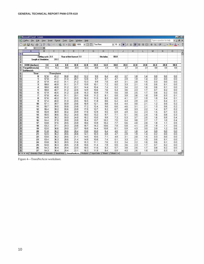
TreesPerAcre worksheet—This worksheet (fig. 4) shows the number of trees per

acre, by species and tree diameter class, for each year of simulation under the

Lexen stocking standard and a 20-year cutting cycle. Scrolling to the right reveals

the trees-per-acre distribution for hardwood species. The underlined numbers

represent the year of harvest and the number of trees per acre just after the harvest.

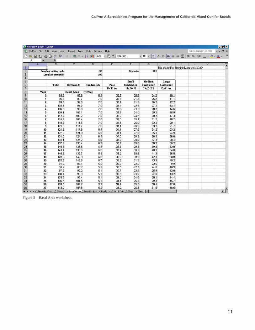
Basal area worksheet—This worksheet (fig. 5) shows, for each simulated year, the

total stand basal area, the stand basal area by species group, and the stand basal

area by timber size category: poles (trees from 5 to 11 in d.b.h.), small sawtimber

(trees from 11 to 15 in d.b.h.), medium sawtimber (trees from 15 to 21 in d.b.h.),

and large sawtimber (trees 21 in d.b.h. and larger). Underlined numbers show the

year of harvest and the basal areas just after harvest.

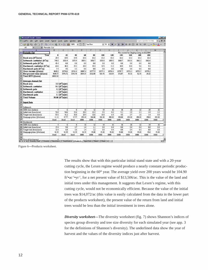
Products worksheet—The upper part of the products worksheet (fig. 6) shows data

for each harvest in terms of basal area cut, gross income, total net present value

(NPV), the pole and sawtimber volumes cut for each species group, and the annual

production in basal area and volume cut. The volumes are computed from equa-

tions linking tree volume to tree diameter, stand basal area, and site index (app. 2).

The lower part is a copy of the input data for reference only.


10

Figure 4—TreesPerAcre worksheet.


11

Figure 5—Basal Area worksheet.


12

The results show that with this particular initial stand state and with a 20-year

cutting cycle, the Lexen regime would produce a nearly constant periodic produc-

tion beginning in the 60th year. The average yield over 200 years would be 104.90

ft3•ac-1•yr-1, for a net present value of $13,506/ac. This is the value of the land and

initial trees under this management. It suggests that Lexen’s regime, with this

cutting cycle, would not be economically efficient. Because the value of the initial

trees was $14,072/ac (this value is easily calculated from the data in the lower part

of the products worksheet), the present value of the return from land and initial

trees would be less than the initial investment in trees alone.

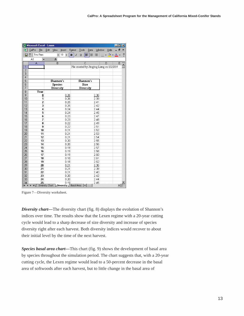
Diversity worksheet—The diversity worksheet (fig. 7) shows Shannon’s indices of

species group diversity and tree size diversity for each simulated year (see app. 3

for the definitions of Shannon’s diversity). The underlined data show the year of

harvest and the values of the diversity indices just after harvest.

Figure 6—Products worksheet.


13

Figure 7—Diversity worksheet.

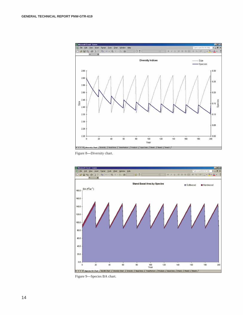
Diversity chart—The diversity chart (fig. 8) displays the evolution of Shannon’s

indices over time. The results show that the Lexen regime with a 20-year cutting

cycle would lead to a sharp decrease of size diversity and increase of species

diversity right after each harvest. Both diversity indices would recover to about

their initial level by the time of the next harvest.

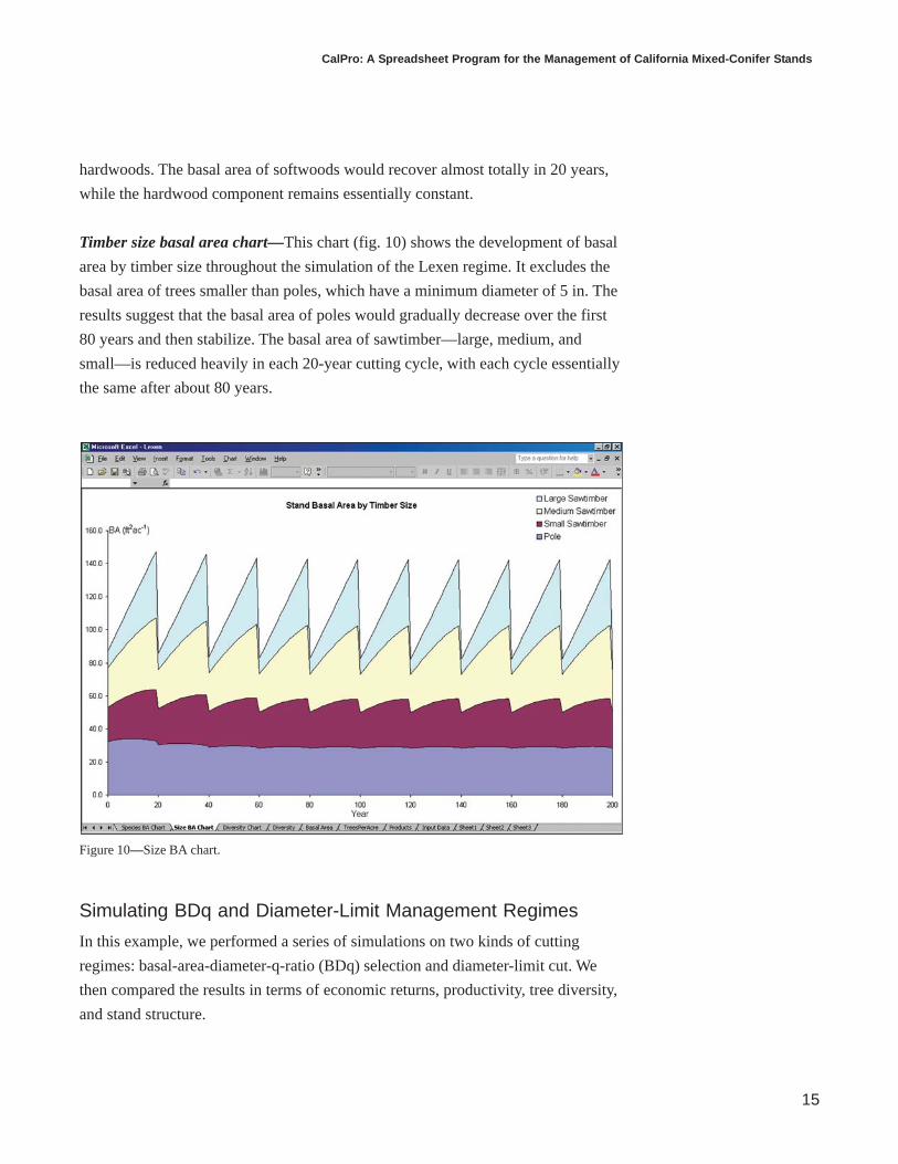
Species basal area chart—This chart (fig. 9) shows the development of basal area

by species throughout the simulation period. The chart suggests that, with a 20-year

cutting cycle, the Lexen regime would lead to a 50-percent decrease in the basal

area of softwoods after each harvest, but to little change in the basal area of


14

Figure 8—Diversity chart.

Figure 9—Species BA chart.


15

hardwoods. The basal area of softwoods would recover almost totally in 20 years,

while the hardwood component remains essentially constant.

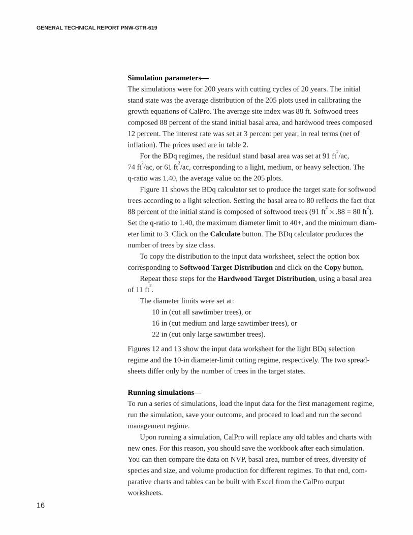
Timber size basal area chart—This chart (fig. 10) shows the development of basal

area by timber size throughout the simulation of the Lexen regime. It excludes the

basal area of trees smaller than poles, which have a minimum diameter of 5 in. The

results suggest that the basal area of poles would gradually decrease over the first

80 years and then stabilize. The basal area of sawtimber—large, medium, and

small—is reduced heavily in each 20-year cutting cycle, with each cycle essentially

the same after about 80 years.

Simulating BDq and Diameter-Limit Management Regimes

In this example, we performed a series of simulations on two kinds of cutting

regimes: basal-area-diameter-q-ratio (BDq) selection and diameter-limit cut. We

then compared the results in terms of economic returns, productivity, tree diversity,

and stand structure.

Figure 10—Size BA chart.


16

Simulation parameters—

The simulations were for 200 years with cutting cycles of 20 years. The initial

stand state was the average distribution of the 205 plots used in calibrating the

growth equations of CalPro. The average site index was 88 ft. Softwood trees

composed 88 percent of the stand initial basal area, and hardwood trees composed

12 percent. The interest rate was set at 3 percent per year, in real terms (net of

inflation). The prices used are in table 2.

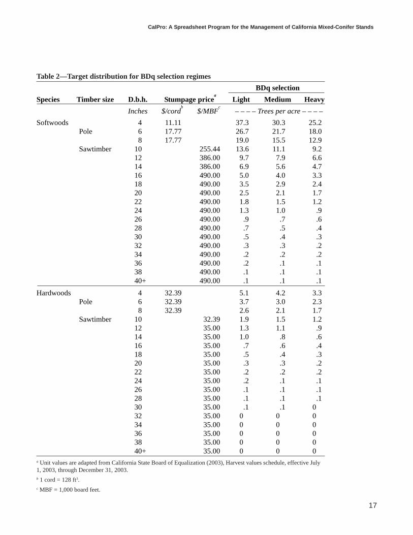
For the BDq regimes, the residual stand basal area was set at 91 ft2/ac,

74 ft2/ac, or 61 ft

2/ac, corresponding to a light, medium, or heavy selection. The

q-ratio was 1.40, the average value on the 205 plots.

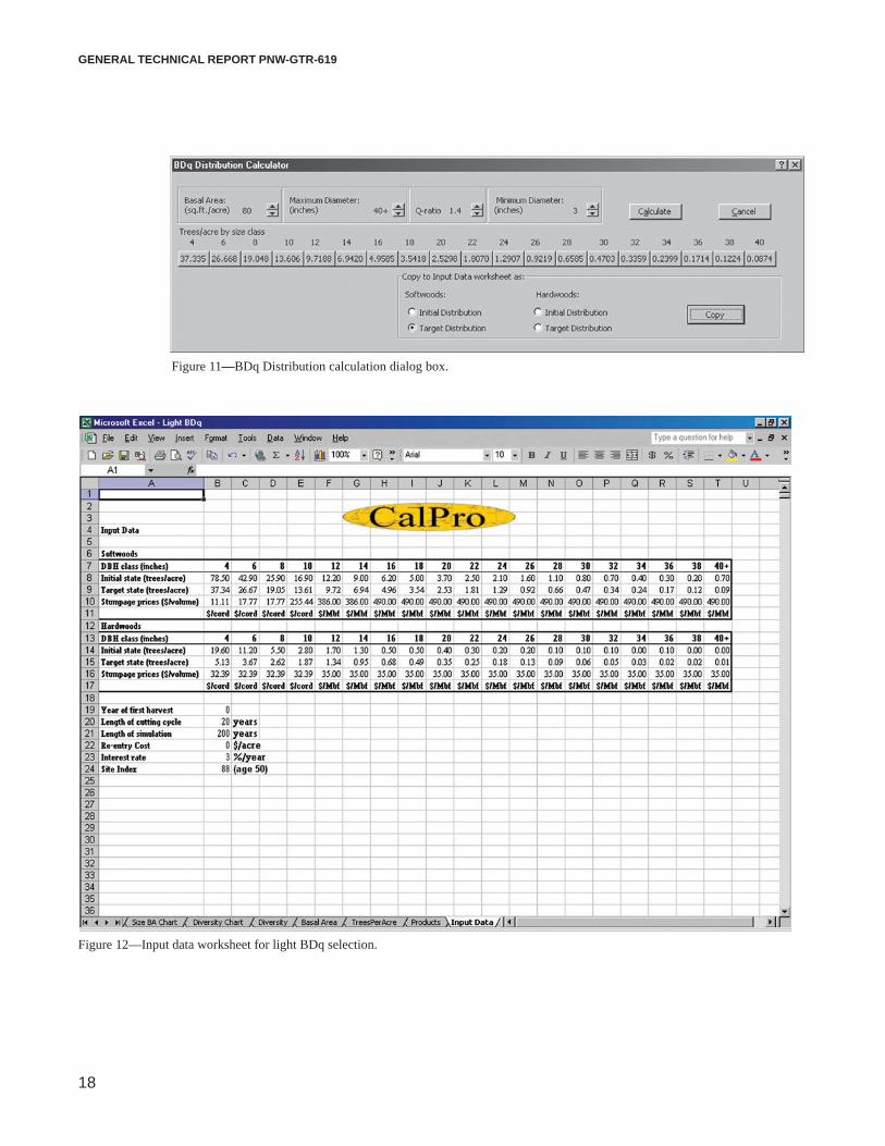
Figure 11 shows the BDq calculator set to produce the target state for softwood

trees according to a light selection. Setting the basal area to 80 reflects the fact that

88 percent of the initial stand is composed of softwood trees (91 ft2 × .88 = 80 ft

2).

Set the q-ratio to 1.40, the maximum diameter limit to 40+, and the minimum diam-

eter limit to 3. Click on the Calculate button. The BDq calculator produces the

number of trees by size class.

To copy the distribution to the input data worksheet, select the option box

corresponding to Softwood Target Distribution and click on the Copy button.

Repeat these steps for the Hardwood Target Distribution, using a basal area

of 11 ft2.

The diameter limits were set at:

10 in (cut all sawtimber trees), or

16 in (cut medium and large sawtimber trees), or

22 in (cut only large sawtimber trees).

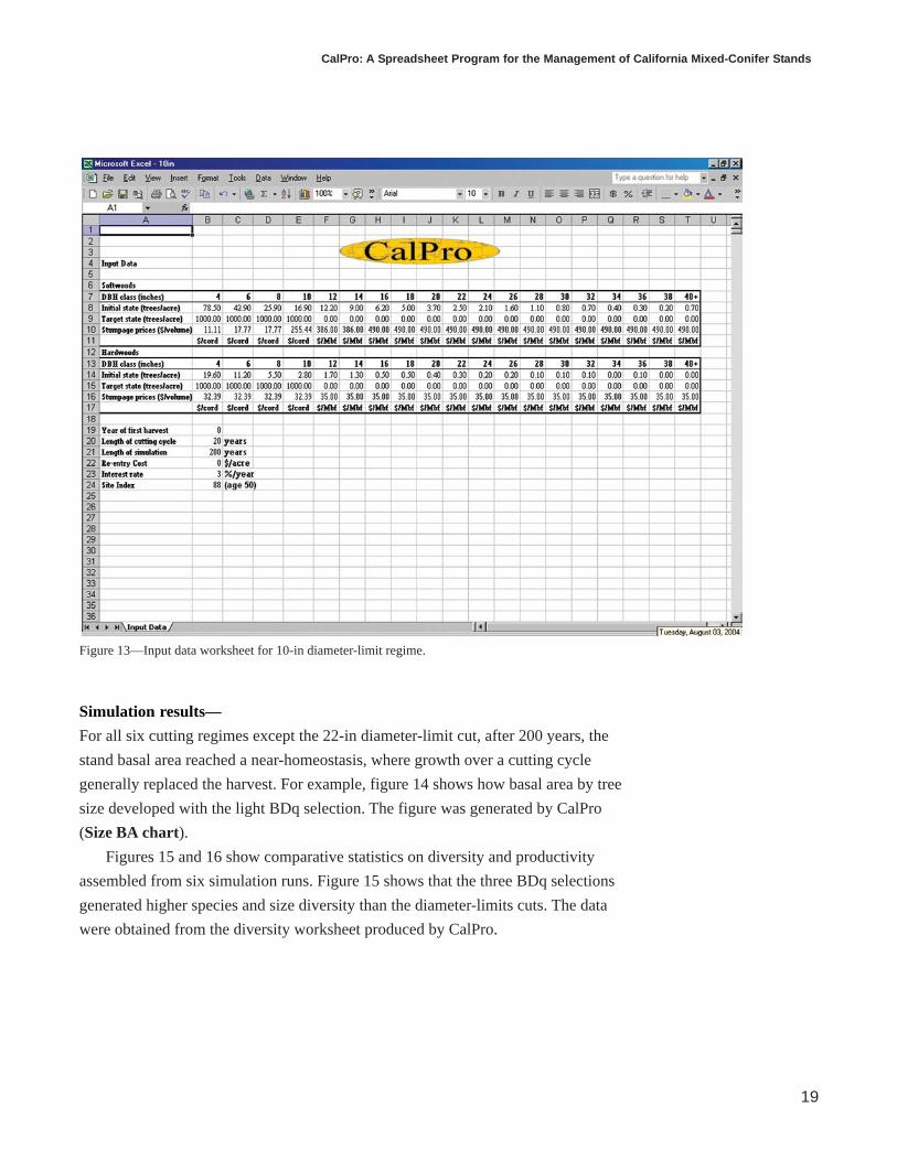
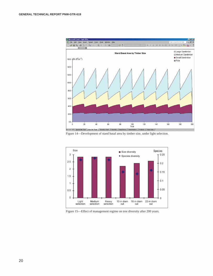
Figures 12 and 13 show the input data worksheet for the light BDq selection

regime and the 10-in diameter-limit cutting regime, respectively. The two spread-

sheets differ only by the number of trees in the target states.

Running simulations—

To run a series of simulations, load the input data for the first management regime,

run the simulation, save your outcome, and proceed to load and run the second

management regime.

Upon running a simulation, CalPro will replace any old tables and charts with

new ones. For this reason, you should save the workbook after each simulation.

You can then compare the data on NVP, basal area, number of trees, diversity of

species and size, and volume production for different regimes. To that end, com-

parative charts and tables can be built with Excel from the CalPro output

worksheets.


17

Table 2—Target distribution for BDq selection regimes

BDq selection

Species Timber size D.b.h. Stumpage pricea

Light Medium Heavy

Inches $/cordb

$/MBFc

– – – – Trees per acre – – – –

Softwoods 4 11.11 37.3 30.3 25.2Pole 6 17.77 26.7 21.7 18.0

8 17.77 19.0 15.5 12.9Sawtimber 10 255.44 13.6 11.1 9.2

12 386.00 9.7 7.9 6.614 386.00 6.9 5.6 4.716 490.00 5.0 4.0 3.318 490.00 3.5 2.9 2.420 490.00 2.5 2.1 1.722 490.00 1.8 1.5 1.224 490.00 1.3 1.0 .926 490.00 .9 .7 .628 490.00 .7 .5 .430 490.00 .5 .4 .332 490.00 .3 .3 .234 490.00 .2 .2 .236 490.00 .2 .1 .138 490.00 .1 .1 .1

40+ 490.00 .1 .1 .1

Hardwoods 4 32.39 5.1 4.2 3.3Pole 6 32.39 3.7 3.0 2.3

8 32.39 2.6 2.1 1.7Sawtimber 10 32.39 1.9 1.5 1.2

12 35.00 1.3 1.1 .914 35.00 1.0 .8 .616 35.00 .7 .6 .418 35.00 .5 .4 .320 35.00 .3 .3 .222 35.00 .2 .2 .224 35.00 .2 .1 .126 35.00 .1 .1 .128 35.00 .1 .1 .130 35.00 .1 .1 032 35.00 0 0 034 35.00 0 0 036 35.00 0 0 038 35.00 0 0 0

40+ 35.00 0 0 0a Unit values are adapted from California State Board of Equalization (2003), Harvest values schedule, effective July1, 2003, through December 31, 2003.b 1 cord = 128 ft3.c MBF = 1,000 board feet.


18

Figure 11—BDq Distribution calculation dialog box.

Figure 12—Input data worksheet for light BDq selection.


19

Figure 13—Input data worksheet for 10-in diameter-limit regime.

Simulation results—

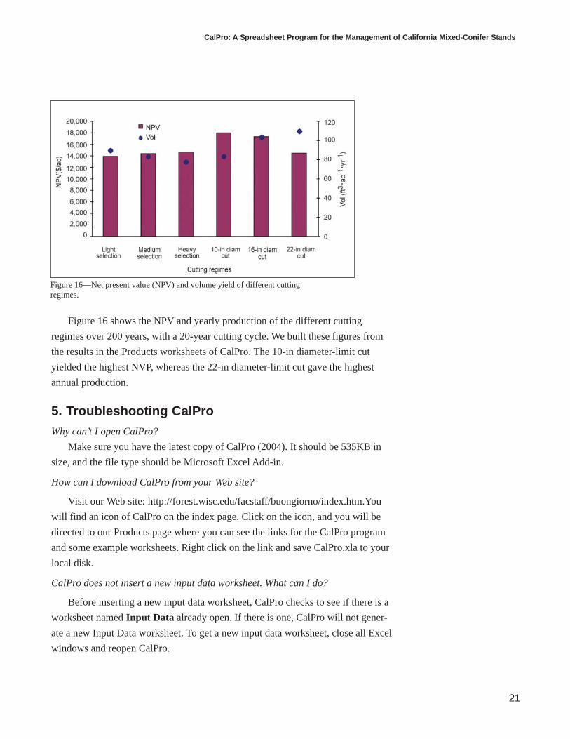
For all six cutting regimes except the 22-in diameter-limit cut, after 200 years, the

stand basal area reached a near-homeostasis, where growth over a cutting cycle

generally replaced the harvest. For example, figure 14 shows how basal area by tree

size developed with the light BDq selection. The figure was generated by CalPro

(Size BA chart).

Figures 15 and 16 show comparative statistics on diversity and productivity

assembled from six simulation runs. Figure 15 shows that the three BDq selections

generated higher species and size diversity than the diameter-limits cuts. The data

were obtained from the diversity worksheet produced by CalPro.


20

Figure 14—Development of stand basal area by timber size, under light selection.

Figure 15—Effect of management regime on tree diversity after 200 years.


21

Figure 16 shows the NPV and yearly production of the different cutting

regimes over 200 years, with a 20-year cutting cycle. We built these figures from

the results in the Products worksheets of CalPro. The 10-in diameter-limit cut

yielded the highest NVP, whereas the 22-in diameter-limit cut gave the highest

annual production.

5. Troubleshooting CalProWhy can’t I open CalPro?

Make sure you have the latest copy of CalPro (2004). It should be 535KB in

size, and the file type should be Microsoft Excel Add-in.

How can I download CalPro from your Web site?

Visit our Web site: http://forest.wisc.edu/facstaff/buongiorno/index.htm.You

will find an icon of CalPro on the index page. Click on the icon, and you will be

directed to our Products page where you can see the links for the CalPro program

and some example worksheets. Right click on the link and save CalPro.xla to your

local disk.

CalPro does not insert a new input data worksheet. What can I do?

Before inserting a new input data worksheet, CalPro checks to see if there is a

worksheet named Input Data already open. If there is one, CalPro will not gener-

ate a new Input Data worksheet. To get a new input data worksheet, close all Excel

windows and reopen CalPro.

Figure 16—Net present value (NPV) and volume yield of different cuttingregimes.


22

Why is there no BDq calculator in the example worksheets?

The example workbooks contain only the input data. After you have installed

CalPro, the BDq calculator icon will appear in the new input data worksheet. At

that point, you can copy data from the example workbooks into the input data

worksheet.

Why is the BDq calculator not working?

CalPro must be open to use the BDq calculator. To use the BDq calculator on a

previously saved input data worksheet, CalPro must be in the Excel menu bar.

Why can’t I copy all the content from the example worksheet to the input data

worksheet?

All the cells of the input data worksheet are protected except those that need

entries (marked with ? marks). Copy only the data from the example worksheet and

paste them to the corresponding locations in the input data worksheet.

For further assistance, or to send us your comments, please visit our Web site

at http://forest.wisc.edu/facstaff/buongiorno/index.htm, or contact us through

[email protected].

AcknowledgmentsThe research leading to this paper was supported, in part, by the USDA Forest

Service, Pacific Northwest Research Station, by USDA-CSREES grant 2001-

35108-10673, and by the School of Natural Resources, University of Wisconsin,

Madison. We thank Jeremy Fried for his participation in the research leading to the

growth-and-yield model underlying CalPro. The authors take sole responsibility for

any error or omission.

Metric EquivalentsWhen you know: Multiply by: To find:

Inches (in) 2.54 Centimeters (cm)

Feet (ft) .305 Meters (m)

Square feet (ft2) .093 Square meters (m2)

Square feet per acre (ft2/ac) .2296 Square meters per hectare (m2/ha)

Cubic feet (ft3) .0283 Cubic meters (m3)


23

Literature CitedAlexander, R.R.; Edminster, C.B. 1976. Regulation and control under uneven-

aged management. In: Uneven-aged silviculture and management in the

Western United States. Proceedings of an in-service workshop. Washington,

DC: U.S. Department of Agriculture, Forest Service, Timber Management

Research: 118-131.

Barbour, M.G.; Major, J. 1977. Introduction. In: Barbour, M.G.; Major, J., eds.

Terrestrial vegetation of California. New York: John Wiley and Sons: 3-10.

California State Board of Equalization. 2003. Harvest values schedule, effective

July 1, 2003 through December 31, 2003. Sacramento, CA. 6 p.

DeBell, D.S.; Franklin, J.F. 1987. Old-growth Douglas-fir and western hemlock:

a 36-year record of growth and mortality. Western Journal of Applied Forestry.

2: 111-114.

Forest Inventory and Analysis. 2000. California inventory data, June 19, 2000

[CD-ROM]. Portland, OR: U.S. Department of Agriculture, Forest Service,

Pacific Northwest Research Station.

Hanson, E.J.; Azuma, D.L.; Hiserote, B.A. 2002. Site index equations and mean

annual increment equations for the Pacific Northwest Research Station Forest

Inventory and Analysis, 1985-2001. Res. Note PNW-RN-533. Portland, OR:

U.S. Department of Agriculture, Forest Service, Pacific Northwest Research

Station. 24 p.

Hiserote, B.; Waddell, K. 2003. The PNW-FIA integrated database user guide.

A database of forest inventory information for California, Oregon and

Washington, V 1.3. Portland, OR: U.S. Department of Agriculture, Forest

Service, Pacific Northwest Research Station, Forest Inventory and Analysis.

10 p.

Liang, J.J.; Buongiorno, J.; Kolbe, A.; Schulte, B. 2004. NorthPro: a spreadsheet

program for the management of uneven-aged northern hardwood stands.

Madison, WI: University of Wisconsin-Madison, Department of Forest Ecol-

ogy and Management. 36 p.

Little, E.L. 1979. Checklist of United States trees (native and naturalized). Agric.

Handb. 541. Washington, DC: U.S. Department of Agriculture, Forest Service.

375 p.

Lu, H.C.; Buongiorno, J. 1993. Long- and short-term effects of alternative cutting

regimes on economic returns and ecological diversity in mixed-species forests.

Forest Ecology and Management. 58: 173-192.


24

Ralston, R.; Buongiorno, J.; Schulte, B.; Fried, J. 2003. WestPro: a computer

program for simulating uneven-aged Douglas-fir stand growth and yield in the

Pacific Northwest. Gen. Tech. Rep. PNW-GTR-574. Portland, OR: U.S.

Department of Agriculture, Forest Service, Pacific Northwest Research Station.

25 p.

Schmidt, T.L. 1998. Wisconsin forest statistics, 1996. Resour. Bull. NC-183.

St. Paul, MN: U.S. Department of Agriculture, Forest Service, North Central

Forest Experiment Station. 150 p.

Schulte, B.; Buongiorno, J.; Lin, C.R.; Skog, K. 1998. SouthPro: a computer

program for managing uneven-aged loblolly pine stands. Gen. Tech. Rep.

FPL-GTR-112. Madison, WI: U.S. Department of Agriculture, Forest Service,

Forest Products Laboratory. 47 p.

U.S. Government Printing Office [USGPO]. 2004. Economic report of the

President. Washington, DC. 417 p.


25

Appendix 1—CalPro DataThe data to calibrate the model used by CalPro came from 205 permanent plots

measured during the last two Forest Inventory and Analysis (2000) surveys con-

ducted by the Portland Inventory and Economics Program of the Pacific Northwest

Research Station. The surveys were conducted in the 1980s and 1990s in forests in

the Sierra Nevada Mountains; national forests and parks were not included in the

sample.

The plots were in the mixed-conifer forest type and in uneven-aged stands

(fewer than 70 percent of the trees differed by less than 30 years in age [Hiserote

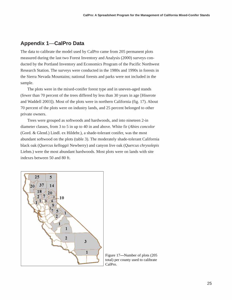
and Waddell 2003]). Most of the plots were in northern California (fig. 17). About

70 percent of the plots were on industry lands, and 25 percent belonged to other

private owners.

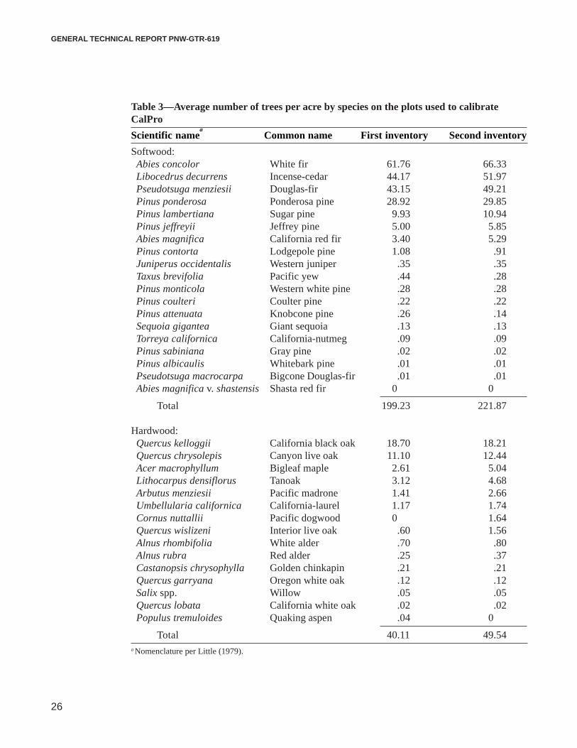
Trees were grouped as softwoods and hardwoods, and into nineteen 2-in

diameter classes, from 3 to 5 in up to 40 in and above. White fir (Abies concolor

(Gord. & Glend.) Lindl. ex Hildebr.), a shade-tolerant conifer, was the most

abundant softwood on the plots (table 3). The moderately shade-tolerant California

black oak (Quercus kelloggii Newberry) and canyon live oak (Quercus chrysolepis

Liebm.) were the most abundant hardwoods. Most plots were on lands with site

indexes between 50 and 80 ft.

Figure 17—Number of plots (205total) per county used to calibrateCalPro.


26

Table 3—Average number of trees per acre by species on the plots used to calibrateCalPro

Scientific namea

Common name First inventory Second inventory

Softwood:Abies concolor White fir 61.76 66.33Libocedrus decurrens Incense-cedar 44.17 51.97Pseudotsuga menziesii Douglas-fir 43.15 49.21Pinus ponderosa Ponderosa pine 28.92 29.85Pinus lambertiana Sugar pine 9.93 10.94Pinus jeffreyii Jeffrey pine 5.00 5.85Abies magnifica California red fir 3.40 5.29Pinus contorta Lodgepole pine 1.08 .91Juniperus occidentalis Western juniper .35 .35Taxus brevifolia Pacific yew .44 .28Pinus monticola Western white pine .28 .28Pinus coulteri Coulter pine .22 .22Pinus attenuata Knobcone pine .26 .14Sequoia gigantea Giant sequoia .13 .13Torreya californica California-nutmeg .09 .09Pinus sabiniana Gray pine .02 .02Pinus albicaulis Whitebark pine .01 .01Pseudotsuga macrocarpa Bigcone Douglas-fir .01 .01Abies magnifica v. shastensis Shasta red fir 0 0

Total 199.23 221.87

Hardwood:Quercus kelloggii California black oak 18.70 18.21Quercus chrysolepis Canyon live oak 11.10 12.44Acer macrophyllum Bigleaf maple 2.61 5.04Lithocarpus densiflorus Tanoak 3.12 4.68Arbutus menziesii Pacific madrone 1.41 2.66Umbellularia californica California-laurel 1.17 1.74Cornus nuttallii Pacific dogwood 0 1.64Quercus wislizeni Interior live oak .60 1.56Alnus rhombifolia White alder .70 .80Alnus rubra Red alder .25 .37Castanopsis chrysophylla Golden chinkapin .21 .21Quercus garryana Oregon white oak .12 .12Salix spp. Willow .05 .05Quercus lobata California white oak .02 .02Populus tremuloides Quaking aspen .04 0

Total 40.11 49.54a Nomenclature per Little (1979).


27

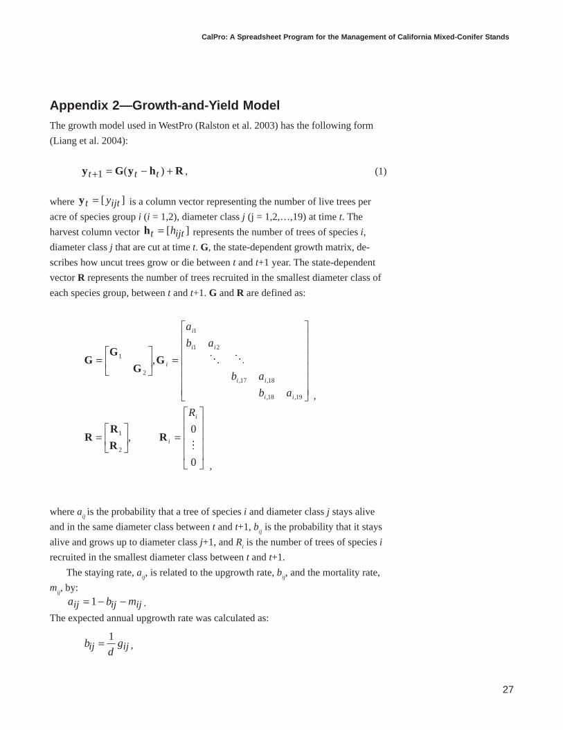
Appendix 2—Growth-and-Yield ModelThe growth model used in WestPro (Ralston et al. 2003) has the following form

(Liang et al. 2004):

RhyGy +−=+ )(1 ttt , (1)

where ][ ijtt y=y is a column vector representing the number of live trees per

acre of species group i (i = 1,2), diameter class j (j = 1,2,…,19) at time t. The

harvest column vector ][ ijtt h=h represents the number of trees of species i,

diameter class j that are cut at time t. G, the state-dependent growth matrix, de-

scribes how uncut trees grow or die between t and t+1 year. The state-dependent

vector R represents the number of trees recruited in the smallest diameter class of

each species group, between t and t+1. G and R are defined as:

=

=

=

=

0

0,

,

2

1

19,18,

18,17,

21

1

2

1

i

i

ii

ii

ii

i

i

R

ab

ab

ab

a

RR

RR

GG

GG

where aij is the probability that a tree of species i and diameter class j stays alive

and in the same diameter class between t and t+1, bij is the probability that it stays

alive and grows up to diameter class j+1, and Ri is the number of trees of species i

recruited in the smallest diameter class between t and t+1.

The staying rate, aij, is related to the upgrowth rate, b

ij, and the mortality rate,

mij, by:

ijijij mba −−= 1 .

The expected annual upgrowth rate was calculated as:

ijij gd

b1= ,

,

,


28

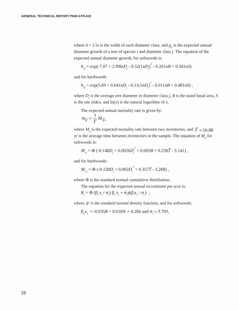
where d = 2 in is the width of each diameter class, and gij is the expected annual

diameter growth of a tree of species i and diameter class j. The equation of the

expected annual diameter growth, for softwoods is:

b1j = exp(-7.07 + 2.99lnD

j - 0.52(1nD

j)

2 - 0.261nB + 0.581nS)

and for hardwoods:

b2j = exp(5.69 + 0.641nD

j - 0.11(1nD

j)

2 - 0.011nB + 0.481nS) ,

where Dj is the average tree diameter in diameter class j, B is the stand basal area, S

is the site index, and ln(x) is the natural logarithm of x.

The expected annual mortality rate is given by:

ijij MT

m1= ,

where Mij is the expected mortality rate between two inventories, and 88.10=T

yr is the average time between inventories in the sample. The equation of Mij for

softwoods is:

M1j = Φ (-0.148D

j + 0.0026D

j

2 + 0.005B + 0.238T - 3.141) ,

and for hardwoods:

M2 j

= Φ (-0.138Dj + 0.002D

j

2 + 0.357T - 3.268) ,

where Φ is the standard normal cumulative distribution.

The equation for the expected annual recruitment per acre is:

Ri = Φ (β

i x

i / σ

i) β

i x

i + σ

iφ(β

ix

i / σ

i ) ,

where φ is the standard normal density function, and for softwoods:

β1x

1 =

-0.035B + 0.018N + 4.266 and σ1 = 5.703,


29

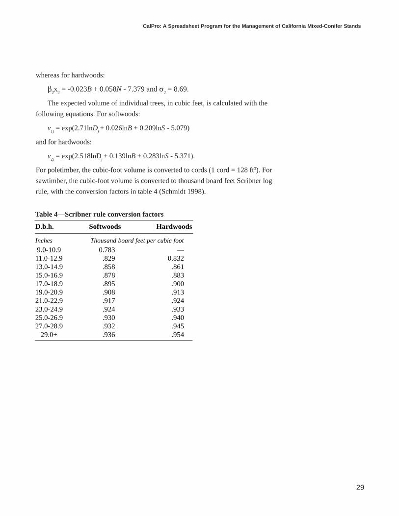
whereas for hardwoods:

β2x

2 = -0.023B + 0.058N - 7.379 and σ

2 = 8.69.

The expected volume of individual trees, in cubic feet, is calculated with the

following equations. For softwoods:

v1j = exp(2.71lnD

j + 0.026lnB + 0.209lnS - 5.079)

and for hardwoods:

v2j = exp(2.518lnD

j + 0.139lnB + 0.283lnS - 5.371).

For poletimber, the cubic-foot volume is converted to cords (1 cord = 128 ft3). For

sawtimber, the cubic-foot volume is converted to thousand board feet Scribner log

rule, with the conversion factors in table 4 (Schmidt 1998).

Table 4—Scribner rule conversion factors

D.b.h. Softwoods Hardwoods

Inches Thousand board feet per cubic foot

9.0-10.9 0.783 —11.0-12.9 .829 0.83213.0-14.9 .858 .86115.0-16.9 .878 .88317.0-18.9 .895 .90019.0-20.9 .908 .91321.0-22.9 .917 .92423.0-24.9 .924 .93325.0-26.9 .930 .94027.0-28.9 .932 .945

29.0+ .936 .954


30

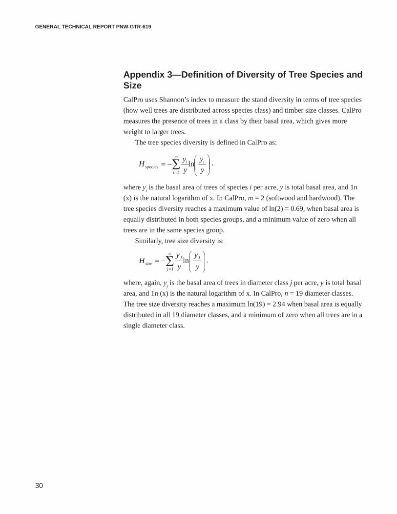
Appendix 3—Definition of Diversity of Tree Species andSizeCalPro uses Shannon’s index to measure the stand diversity in terms of tree species

(how well trees are distributed across species class) and timber size classes. CalPro

measures the presence of trees in a class by their basal area, which gives more

weight to larger trees.

The tree species diversity is defined in CalPro as:

where yi is the basal area of trees of species i per acre, y is total basal area, and 1n

(x) is the natural logarithm of x. In CalPro, m = 2 (softwood and hardwood). The

tree species diversity reaches a maximum value of ln(2) = 0.69, when basal area is

equally distributed in both species groups, and a minimum value of zero when all

trees are in the same species group.

Similarly, tree size diversity is:

where, again, yj is the basal area of trees in diameter class j per acre, y is total basal

area, and 1n (x) is the natural logarithm of x. In CalPro, n = 19 diameter classes.

The tree size diversity reaches a maximum ln(19) = 2.94 when basal area is equally

distributed in all 19 diameter classes, and a minimum of zero when all trees are in a

single diameter class.

−= ∑= y

y

y

yH i

m

1i

ispecies ln

−= ∑

= y

y

y

yH j

n

1j

jsize ln ,

,


31

GlossaryBA chart—A CalPro-generated chart showing, for a selected range of years, the

per-acre basal area of softwoods, hardwoods, and the whole stand.

BDq distribution—A tree distribution, by diameter class, defined by a stand basal

area (B), a maximum and minimum tree diameter (D), and a q-ratio (q), the

ratio of the number of trees in a given diameter class to the number of trees in

the next larger class.

cutting cycle—The number of years between successive harvests. For two-cut

silvicultural systems, this is also equal to the number of years between succes-

sive harvests.

diameter class—One of nineteen 2-in diameter at breast height (d.b.h.) categories

used by CalPro to classify trees by size. Diameter classes range from 4 to 40+

in, with each class denoted by its midpoint diameter. Diameter class 4 is for

trees with diameters from 3 to less than 5 in. The 40+ in class is for all trees

39 in in diameter and larger.

diversity chart—A CalPro-generated chart showing changes in the Shannon index

of species or size diversity over a selected range of years.

hardwood—See species groups.

initial stand state—The number of live trees per acre, by species and size, at the

start of a simulation.

input data worksheet—A worksheet to enter the data for running a CalPro

simulation.

Microsoft Excel add-in—A command, function, or software program that runs

within Microsoft Excel and adds special capabilities. CalPro is an add-in.

net present value (NPV)—The net revenue discounted to the present.

pole-size trees—Trees suitable for the production of poletimber but too small to

produce saw logs. In CalPro, these include trees from 5 to less than 11 in.

preharvest stand state—The number of live trees per acre, by species and size,

immediately before a harvest.

products worksheet—A CalPro output worksheet that shows, for each harvest, the

basal area cut, the volume of poles and sawtimber removed by species group,

the gross income generated, and the NPV of the harvest, as well as the total

NPV of the stand and its mean annual production in terms of basal area cut and

volumes harvested, on a per-acre basis.

re-entry costs—Costs per acre associated with each harvest that are not reflected

in the stumpage prices. These may include, e.g., the added expense of marking

the stand for single-tree selection or controlling hardwood competition.


32

sawtimber—Trees suitable for the production of saw logs. CalPro’s marking

guides recognize three classes of sawtimber trees:

(1) Small sawtimber—Trees with d.b.h. of 11 to less than 15 in.

(2) Medium sawtimber—Trees with d.b.h. of 15 to less than 21 in.

(3) Large sawtimber—Trees with d.b.h. of 21 in or larger.

Setup File worksheet—A worksheet to store CalPro setup files. It is typically

hidden.

Setup Files—Collections of related input data that are stored together on a Setup

File worksheet. Setup Files may contain data for initial stand states, target

stand states, cutting cycle parameters, stumpage prices, or fixed costs, and may

be used in varying combinations as input for CalPro simulations.

site index—The average height of a stand’s dominant and codominant trees at age

50 years.

size diversity—The diversity of tree diameter classes as measured by the Shannon

index. With 19 diameter classes, size diversity reaches its maximum value of

2.94 when the basal area or number of trees is distributed evenly among the

diameter classes.

softwood —See species groups.

species diversity—The diversity of species groups as measured by the Shannon

index. With two species classes, species diversity reaches its maximum value

of 0.69 when the basal area or number of trees is distributed evenly among the

species groups.

species groups—The two categories used by CalPro to classify trees by species.

softwoods—Wood from Gymnospermae, mostly coniferous species such as

pine or fir.

hardwoods—Wood from Angiospermae, mostly broad-leaved dicotyledonous

species.

stumpage prices—Prices paid to a landowner for standing timber.

target stand state—The desired number of live trees per acre in each species

group and diameter class after a harvest.

total net present value—The sum of all discounted revenues minus the sum of all

discounted costs.

workbook—The workbook is the normal document or file type in Microsoft Excel.

A workbook is the electronic equivalent of a three-ring binder. Inside work-

books you will find sheets, such as worksheets and chart sheets.

worksheet—Most of the work you do in Excel will be on a worksheet. A

worksheet is a grid of rows and columns. Each cell is the intersection of a row

and a column and has a unique address, or reference.

This page has been left blank intentionally.Document continues on next page.

.

This page has been left blank intentionally.Document continues on next page.

.

Pacific Northwest Research Station

Web site http://www.fs.fed.us/pnwTelephone (503) 808-2592Publication requests (503) 808-2138FAX (503) 808-2130E-mail [email protected] address Publications Distribution

Pacific Northwest Research StationP.O. Box 3890Portland, OR 97208-3890

U.S. Department of AgriculturePacific Northwest Research Station333 S.W. First AvenueP.O. Box 3890Portland, OR 97208-3890

Official BusinessPenalty for Private Use, $300

Documents

CalPro: A Spreadsheet · CalPro: A Spreadsheet Program for the ... a spread-sheet program for the management of ... CalPro is an add-in program developed to work with Microsoft Excel