California State University, Northridge Information ...csunitr/guides/excel/2003/excel_wkgmulti.pdfCalifornia State University, Northridge Information Technology Training Guide Prepared

California State University, Northridge Information Technology Training Guide

Prepared by Tina Actis-Purtee, User Support Services June 13, 2006

ITR’s Technology training guides are the property of California State University, Northridge. They are intended for non-profit educational use only. Please do not use this material without citing the source.

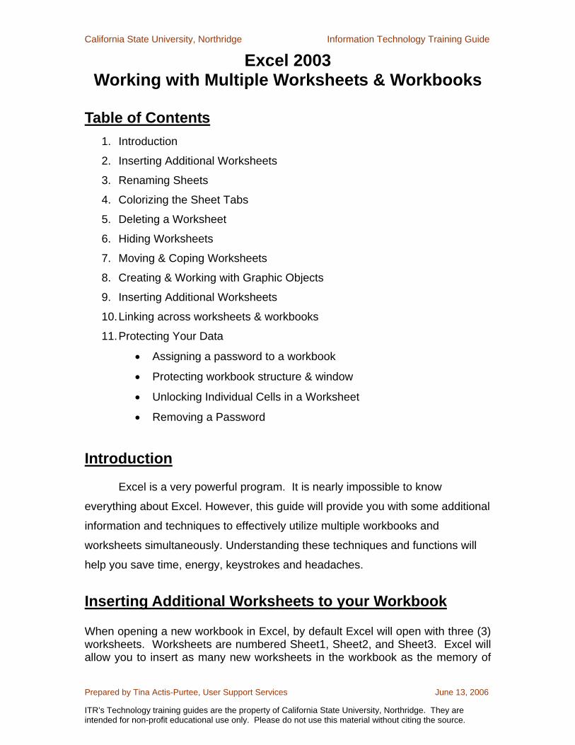
Excel 2003 Working with Multiple Worksheets & Workbooks

Table of Contents

1. Introduction

2. Inserting Additional Worksheets

3. Renaming Sheets

4. Colorizing the Sheet Tabs

5. Deleting a Worksheet

6. Hiding Worksheets

7. Moving & Coping Worksheets

8. Creating & Working with Graphic Objects

9. Inserting Additional Worksheets

10. Linking across worksheets & workbooks

11. Protecting Your Data

• Assigning a password to a workbook

• Protecting workbook structure & window

• Unlocking Individual Cells in a Worksheet

• Removing a Password

Introduction

Excel is a very powerful program. It is nearly impossible to know

everything about Excel. However, this guide will provide you with some additional

information and techniques to effectively utilize multiple workbooks and

worksheets simultaneously. Understanding these techniques and functions will

help you save time, energy, keystrokes and headaches.

Inserting Additional Worksheets to your Workbook

When opening a new workbook in Excel, by default Excel will open with three (3) worksheets. Worksheets are numbered Sheet1, Sheet2, and Sheet3. Excel will allow you to insert as many new worksheets in the workbook as the memory of




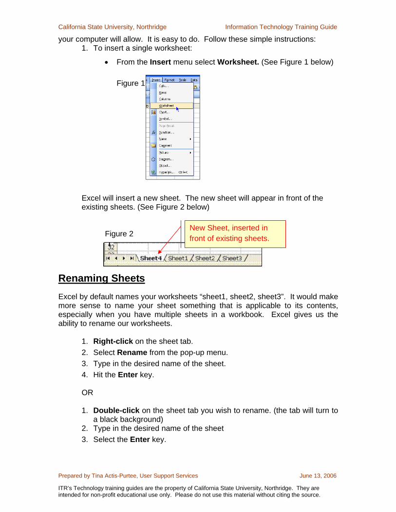
your computer will allow. It is easy to do. Follow these simple instructions: 1. To insert a single worksheet:

• From the Insert menu select Worksheet. (See Figure 1 below)

Figure 1

Excel will insert a new sheet. The new sheet will appear in front of the existing sheets. (See Figure 2 below)

Figure 2

Renaming Sheets Excel by default names your worksheets “sheet1, sheet2, sheet3”. It would make more sense to name your sheet something that is applicable to its contents, especially when you have multiple sheets in a workbook. Excel gives us the ability to rename our worksheets.

1. Right-click on the sheet tab. 2. Select Rename from the pop-up menu. 3. Type in the desired name of the sheet. 4. Hit the Enter key.

OR

1. Double-click on the sheet tab you wish to rename. (the tab will turn to a black background)

2. Type in the desired name of the sheet 3. Select the Enter key.

New Sheet, inserted in front of existing sheets.




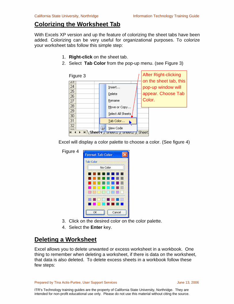
Colorizing the Worksheet Tab

With Excels XP version and up the feature of colorizing the sheet tabs have been added. Colorizing can be very useful for organizational purposes. To colorize your worksheet tabs follow this simple step:

1. Right-click on the sheet tab. 2. Select Tab Color from the pop-up menu. (see Figure 3)

Figure 3

Excel will display a color palette to choose a color. (See figure 4)

Figure 4

3. Click on the desired color on the color palette. 4. Select the Enter key.

Deleting a Worksheet Excel allows you to delete unwanted or excess worksheet in a workbook. One thing to remember when deleting a worksheet, if there is data on the worksheet, that data is also deleted. To delete excess sheets in a workbook follow these few steps:

After Right-clicking on the sheet tab, this pop-up window will appear. Choose Tab Color.




1. Click on the tab of the worksheet you wish to delete. To select

multiple worksheets, hold down the Ctrl key while clicking on the worksheet tabs.

2. From the Edit menu, choose Delete Sheet.

Excel will then delete the selected worksheets

Hiding and Un-hiding a worksheet

Excel gives you the ability to hide worksheets in your workbooks. You might ask, what would I need to hide a worksheet for? Hiding a worksheet may be useful if you do not want others to see it, or if you just want to get it out of the way. When a sheet is hidden, its sheet tab is also hidden.

Hiding a worksheet may prevent casual users from viewing or changing important information in a workbook.

To hide a worksheet: 1. Select the worksheet you wish to hide. 2. From the Format menu, choose Sheet > Hide from the sub-menu

The active worksheet (or selected worksheets) will be hidden from view. Every workbook must have at least one visible sheet, so Excel won’t allow you to hide all the sheets in a workbook.

Un-hiding or revealing a hidden worksheet

1. From the Format menu, choose Sheet t 2. Select Unhide from the sub-menu 3. Excel will display a menu with the hidden worksheets. Double-click

on the hidden worksheet you wish to display.

Moving & Copying Worksheets

Moving a worksheet Excel provides a very easy way to move a sheet from one place to another either within the current workbook or to another workbook.

1. Click the sheet tab you want to move.




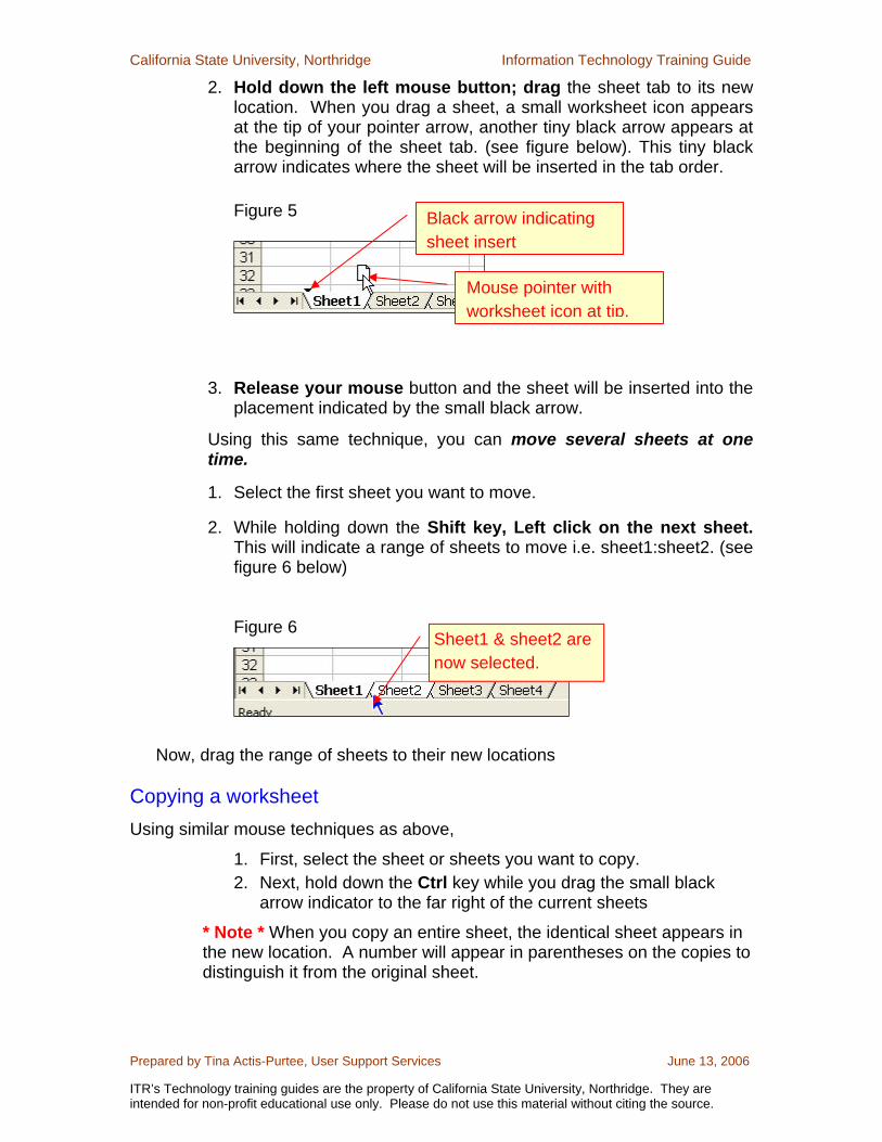
2. Hold down the left mouse button; drag the sheet tab to its new location. When you drag a sheet, a small worksheet icon appears at the tip of your pointer arrow, another tiny black arrow appears at the beginning of the sheet tab. (see figure below). This tiny black arrow indicates where the sheet will be inserted in the tab order.

Figure 5

3. Release your mouse button and the sheet will be inserted into the

placement indicated by the small black arrow.

Using this same technique, you can move several sheets at one time.

1. Select the first sheet you want to move.

2. While holding down the Shift key, Left click on the next sheet. This will indicate a range of sheets to move i.e. sheet1:sheet2. (see figure 6 below)

Figure 6

Now, drag the range of sheets to their new locations

Copying a worksheet Using similar mouse techniques as above,

1. First, select the sheet or sheets you want to copy. 2. Next, hold down the Ctrl key while you drag the small black

arrow indicator to the far right of the current sheets

* Note * When you copy an entire sheet, the identical sheet appears in the new location. A number will appear in parentheses on the copies to distinguish it from the original sheet.

Sheet1 & sheet2 are now selected.

Black arrow indicating sheet insert

Mouse pointer with worksheet icon at tip.




For MAC users:

1. Select the sheet or sheets you want to copy. 2. From the Edit menu choose Move or Copy. 3. In the move or copy dialog box check the “Create a copy” box 4. Click OK.

Moving and Copying Sheets between Workbooks Excel has the ability to move or copy sheets from a current workbook to another open workbook by simply dragging the sheet. Very easy isn’t it.

Moving sheets between workbooks You can use the same methods as described on the previous page to move a worksheet to another workbook.

1. Open both workbooks you will be working in. (see tip below for viewing more than one workbook at a time)

2. Click on the sheet tab you wish to move from workbook 1 to workbook 2.

3. Hold the left mouse button down, Drag the sheet from workbook 1 to where you want it to be in workbook 2. The entire sheet from workbook 1 will be moved to workbook 2. It will no longer be in workbook 1.

*TIP* To view more than one workbook at a time, 1. First open all the workbooks. 2. Next, from the Window pull-down menu, select Arrange, 3. Then from the sub-menu select Tiled.

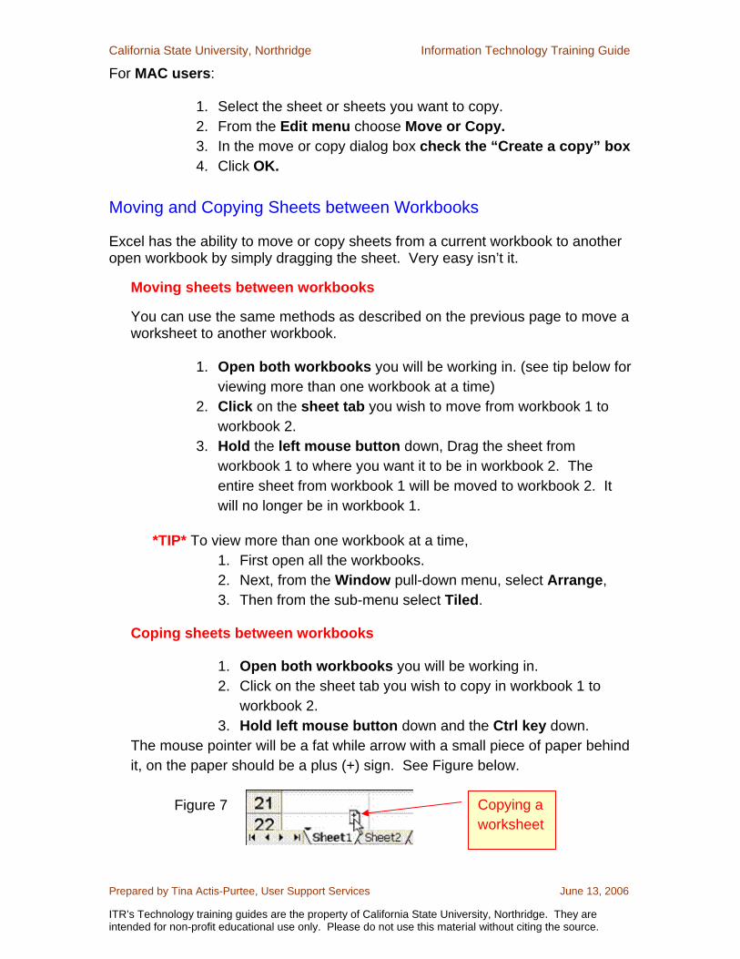
Coping sheets between workbooks

1. Open both workbooks you will be working in. 2. Click on the sheet tab you wish to copy in workbook 1 to

workbook 2. 3. Hold left mouse button down and the Ctrl key down.

The mouse pointer will be a fat while arrow with a small piece of paper behind it, on the paper should be a plus (+) sign. See Figure below.

Figure 7

Copying a worksheet




4. Drag the sheet from workbook 1 to where you want it to be in workbook 2. A copy of the entire sheet is placed in workbook 2.

Creating & Working with Graphic Objects With Microsoft Excel you can create a variety of graphic objects - boxes, lines, circles, ovals, arcs, freeform polygons, test boxes, buttons, and a wide assortment of complex predefined objects called "AutoShapes". You can specify font, pattern, color, and line formats, and you can position objects in relation to the worksheet or to other objects. You can also take pictures of your worksheets and use them in other Excel documents or in documents created in other applications.

This section is intended to acquaint you with MS Excel’s Drawing and Graphic Object capabilities.

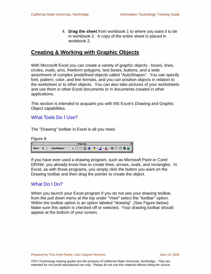
What Tools Do I Use? The "Drawing" toolbar in Excel is all you need.

Figure 8

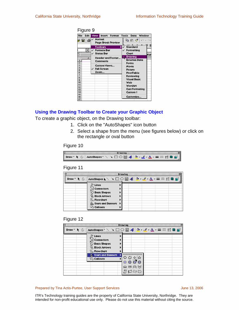
If you have ever used a drawing program, such as Microsoft Paint or Corel DRAW, you already know how to create lines, arrows, ovals, and rectangles. In Excel, as with those programs, you simply click the button you want on the Drawing toolbar and then drag the pointer to create the object. What Do I Do? When you launch your Excel program if you do not see your drawing toolbar, from the pull down menu at the top under "View" select the "toolbar" option. Within the toolbar option is an option labeled "drawing". (See Figure below) Make sure this option is checked off or selected. Your drawing toolbar should appear at the bottom of your screen.




Figure 9

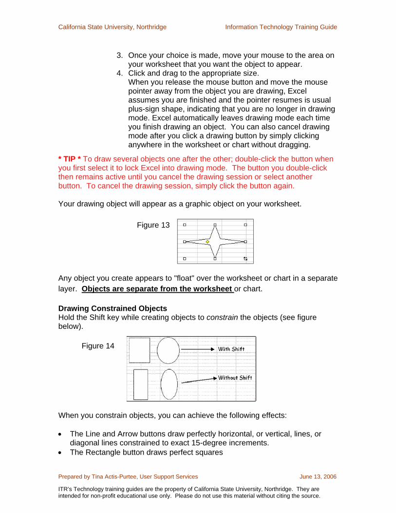
Using the Drawing Toolbar to Create your Graphic Object To create a graphic object, on the Drawing toolbar:

1. Click on the "AutoShapes" icon button 2. Select a shape from the menu (see figures below) or click on

the rectangle or oval button

Figure 10

Figure 11

Figure 12




3. Once your choice is made, move your mouse to the area on your worksheet that you want the object to appear.

4. Click and drag to the appropriate size. When you release the mouse button and move the mouse pointer away from the object you are drawing, Excel assumes you are finished and the pointer resumes is usual plus-sign shape, indicating that you are no longer in drawing mode. Excel automatically leaves drawing mode each time you finish drawing an object. You can also cancel drawing mode after you click a drawing button by simply clicking anywhere in the worksheet or chart without dragging.

* TIP * To draw several objects one after the other; double-click the button when you first select it to lock Excel into drawing mode. The button you double-click then remains active until you cancel the drawing session or select another button. To cancel the drawing session, simply click the button again.

Your drawing object will appear as a graphic object on your worksheet. Figure 13 Any object you create appears to "float" over the worksheet or chart in a separate layer. Objects are separate from the worksheet or chart.

Drawing Constrained Objects Hold the Shift key while creating objects to constrain the objects (see figure below).

Figure 14

When you constrain objects, you can achieve the following effects:

• The Line and Arrow buttons draw perfectly horizontal, or vertical, lines, or diagonal lines constrained to exact 15-degree increments.

• The Rectangle button draws perfect squares




• The Oval button draws perfect circles. • AutoShapes are drawn to predefined, roughly symmetrical constraints.

AutoShapes are widely different things, depending on the shape. Deleting Graphic Objects To delete a graphic object,:

1. Click on the object to select it, 2. Press the "delete" key.

Repeat the steps above to create another Graphic Object.

Sizing, Moving, and Copying Graphic Objects You can change the size, position, and formatting of graphic objects you have created.

Resizing an Object

1. Select the object and position the mouse pointer over a selection handle.

Note: The selection handles appear as little squares around the object, your mouse pointer will change to a two sided arrow pointer.

2. Drag to the new size 3. Release the mouse button

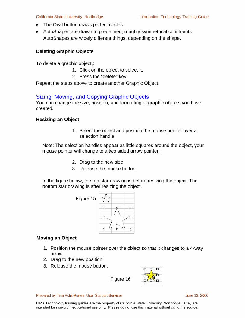
In the figure below, the top star drawing is before resizing the object. The bottom star drawing is after resizing the object.

Figure 15 Moving an Object

1. Position the mouse pointer over the object so that it changes to a 4-way arrow

2. Drag to the new position 3. Release the mouse button.

Figure 16




Copying an Object To copy an object once you have formed the size and shape wanted:

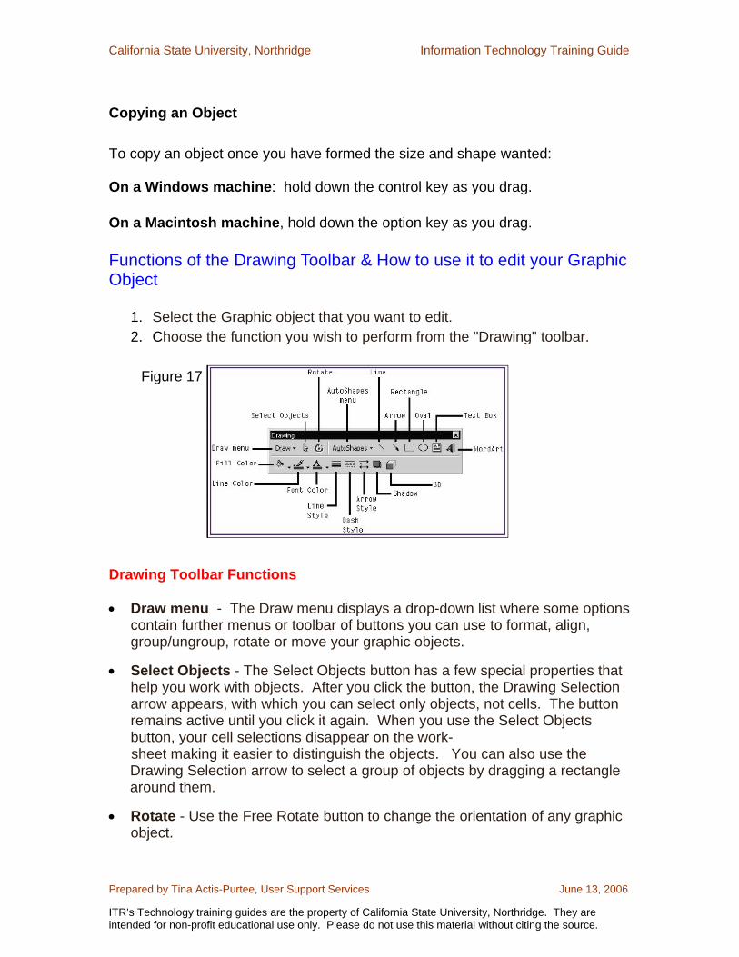
On a Windows machine: hold down the control key as you drag. On a Macintosh machine, hold down the option key as you drag. Functions of the Drawing Toolbar & How to use it to edit your Graphic Object

1. Select the Graphic object that you want to edit. 2. Choose the function you wish to perform from the "Drawing" toolbar.

Figure 17 Drawing Toolbar Functions

• Draw menu - The Draw menu displays a drop-down list where some options contain further menus or toolbar of buttons you can use to format, align, group/ungroup, rotate or move your graphic objects.

• Select Objects - The Select Objects button has a few special properties that help you work with objects. After you click the button, the Drawing Selection arrow appears, with which you can select only objects, not cells. The button remains active until you click it again. When you use the Select Objects button, your cell selections disappear on the worksheet making it easier to distinguish the objects. You can also use the Drawing Selection arrow to select a group of objects by dragging a rectangle around them.

• Rotate - Use the Free Rotate button to change the orientation of any graphic object.




• AutoShapes Menu - The AutoShapes menu displays a drop-down list or toolbar of buttons you can use to create a variety of AutoShapes.

• Line - Select the Line button to draw a straight line

• Arrow - Select the Arrow button to draw a straight arrow of any length.

• Rectangle - Select the Rectangle button to draw a rectangle or a square of any size.

• Oval - Select the Oval button to draw an Oval or a circle of any size.

• Text Box - Click on the Text Box button to insert text in any of your graphic objects.

• WordArt - The WordArt button on the Drawing toolbar opens a palette of formatting styles you can utilize to create impressive graphic objects using text.

• Fill Color, Font Color, & Line Color - These three buttons on the drawing toolbar are tear-off palettes. If you click and drag them away from the toolbar, they become little floating toolbars. The Fill Color and Font Color buttons can be used to format either cells or objects. The Fill color button will allow you to place background color in your object or cell. The Font color button will allow you to change the color of the Text within an object or cell. The Line color button will allow you to change the color of the selected line or object.

• Line Style, Dash Style, and Arrow Style - These three Style buttons allow a selection of commonly used line, dash or arrow styles. Simply click on the option you want.

MS Excel has great graphic capabilities. The Graphic Objects options can be utilized in your daily work for more effective work presentation. Have a little fun and create effective graphic objects.

Linking Information Do you find yourself entering the same information on multiple worksheets? Then having to go in and update this information on each sheet? Frequently, you may have the same information in multiple sheets. Linking can save you time and effort by allowing you to:

Take information on one worksheet and “Link” it to another sheet, therefore only having to enter it one time.

Update information on the source worksheet and it will automatically update the information in the linked cells on the linked worksheets.




This feature can be very handy and save many keystrokes and possible errors. The worksheet page that the information is contained on that you wish to “link” to another page is called the source worksheet. The worksheet that the information is to be linked to is referred to as the target worksheet.

Linking Information between Worksheets in a single Workbook

To link information between two open worksheets, use the following steps:

1. Select the cell(s) of information in the source worksheet you want to link to the target worksheet.

2. Right-click on the selected cell(s) and select Copy from the menu. 3. Go to the target worksheet you want to paste the information to. 4. Select the cell or range on the target worksheet that you want to link

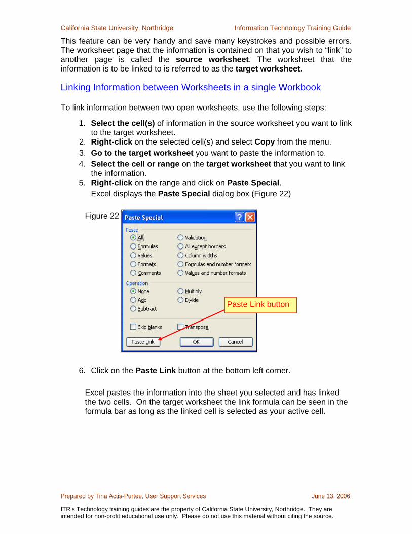
the information. 5. Right-click on the range and click on Paste Special.

Excel displays the Paste Special dialog box (Figure 22)

Figure 22

6. Click on the Paste Link button at the bottom left corner.

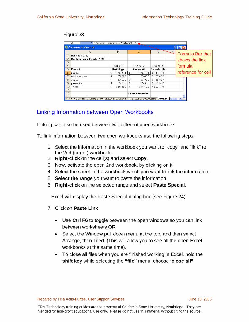
Excel pastes the information into the sheet you selected and has linked the two cells. On the target worksheet the link formula can be seen in the formula bar as long as the linked cell is selected as your active cell.

Paste Link button




Figure 23

Linking Information between Open Workbooks Linking can also be used between two different open workbooks. To link information between two open workbooks use the following steps:

1. Select the information in the workbook you want to “copy” and “link” to the 2nd (target) workbook.

2. Right-click on the cell(s) and select Copy. 3. Now, activate the open 2nd workbook, by clicking on it. 4. Select the sheet in the workbook which you want to link the information. 5. Select the range you want to paste the information. 6. Right-click on the selected range and select Paste Special.

Excel will display the Paste Special dialog box (see Figure 24)

7. Click on Paste Link.

• Use Ctrl F6 to toggle between the open windows so you can link between worksheets OR

• Select the Window pull down menu at the top, and then select Arrange, then Tiled. (This will allow you to see all the open Excel workbooks at the same time).

• To close all files when you are finished working in Excel, hold the shift key while selecting the “file” menu, choose ‘close all”.

Formula Bar that shows the link formula reference for cell




Removing Links between Workbooks You can remove or “freeze” the information in the target area by converting the linked information to values that do not change. To remove a link, follow these steps:

1. Select the linked information in the target sheet. 2. Right-click on the selected information and click on Copy.

Excel will copy the linked information to the Windows clipboard

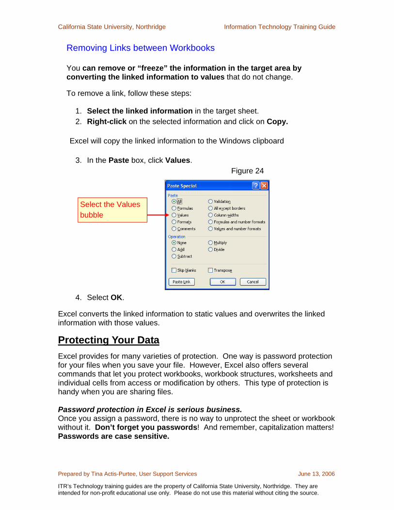
3. In the Paste box, click Values.

Figure 24

4. Select OK. Excel converts the linked information to static values and overwrites the linked information with those values.

Protecting Your Data Excel provides for many varieties of protection. One way is password protection for your files when you save your file. However, Excel also offers several commands that let you protect workbooks, workbook structures, worksheets and individual cells from access or modification by others. This type of protection is handy when you are sharing files. Password protection in Excel is serious business. Once you assign a password, there is no way to unprotect the sheet or workbook without it. Don’t forget you passwords! And remember, capitalization matters! Passwords are case sensitive.

Select the Values bubble




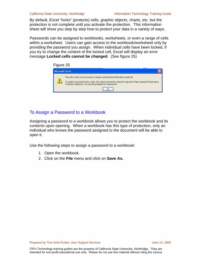
By default, Excel “locks” (protects) cells, graphic objects, charts, etc. but the protection is not complete until you activate the protection. This information sheet will show you step by step how to protect your data in a variety of ways. Passwords can be assigned to workbooks, worksheets, or even a range of cells within a worksheet. Users can gain access to the workbook/worksheet only by providing the password you assign. When individual cells have been locked, if you try to change the content of the locked cell, Excel will display an error message Locked cells cannot be changed. (See figure 25)

Figure 25

To Assign a Password to a Workbook Assigning a password to a workbook allows you to protect the workbook and its contents upon opening. When a workbook has this type of protection, only an individual who knows the password assigned to the document will be able to open it. Use the following steps to assign a password to a workbook:

1. Open the workbook. 2. Click on the File menu and click on Save As.




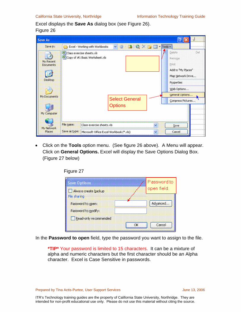
Excel displays the Save As dialog box (see Figure 26). Figure 26

• Click on the Tools option menu. (See figure 26 above). A Menu will appear.

Click on General Options. Excel will display the Save Options Dialog Box. (Figure 27 below)

Figure 27

In the Password to open field, type the password you want to assign to the file.

*TIP* Your password is limited to 15 characters. It can be a mixture of alpha and numeric characters but the first character should be an Alpha character. Excel is Case Sensitive in passwords.

Select General Options




In the Password to modify box, type the password you want to assign to the file.

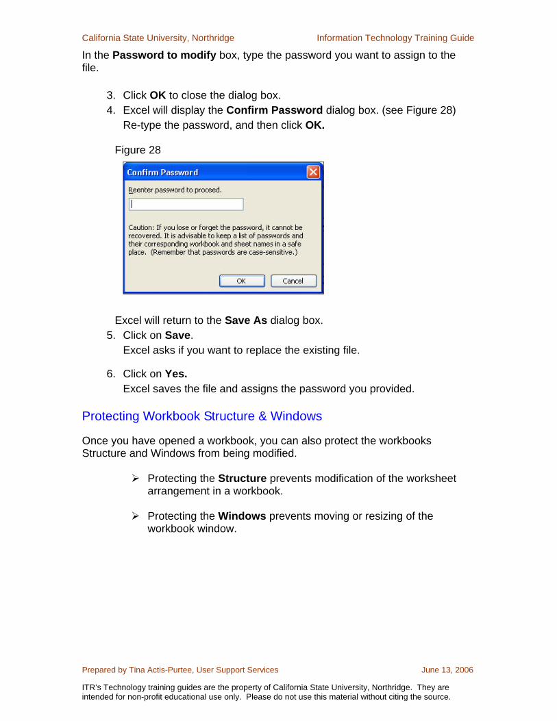
3. Click OK to close the dialog box. 4. Excel will display the Confirm Password dialog box. (see Figure 28)

Re-type the password, and then click OK.

Figure 28

Excel will return to the Save As dialog box. 5. Click on Save.

Excel asks if you want to replace the existing file.

6. Click on Yes. Excel saves the file and assigns the password you provided.

Protecting Workbook Structure & Windows Once you have opened a workbook, you can also protect the workbooks Structure and Windows from being modified.

Protecting the Structure prevents modification of the worksheet arrangement in a workbook.

Protecting the Windows prevents moving or resizing of the

workbook window.




To active these protections:

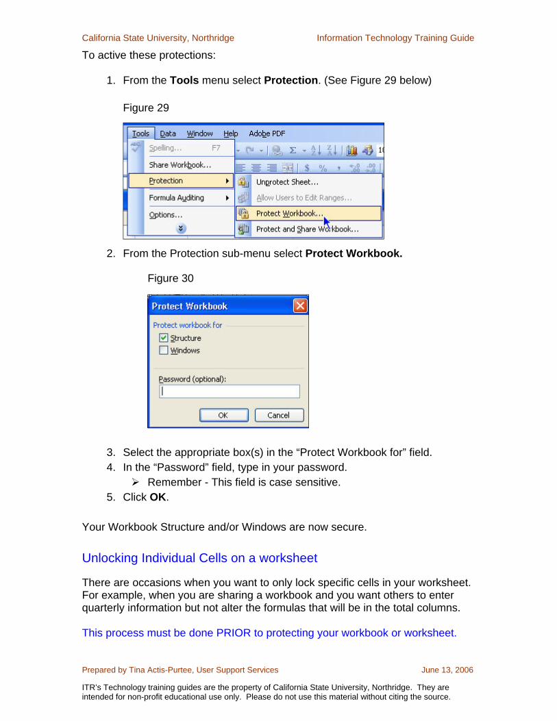
1. From the Tools menu select Protection. (See Figure 29 below) Figure 29

2. From the Protection sub-menu select Protect Workbook.

Figure 30

3. Select the appropriate box(s) in the “Protect Workbook for” field. 4. In the “Password” field, type in your password.

Remember - This field is case sensitive. 5. Click OK.

Your Workbook Structure and/or Windows are now secure. Unlocking Individual Cells on a worksheet There are occasions when you want to only lock specific cells in your worksheet. For example, when you are sharing a workbook and you want others to enter quarterly information but not alter the formulas that will be in the total columns. This process must be done PRIOR to protecting your workbook or worksheet.




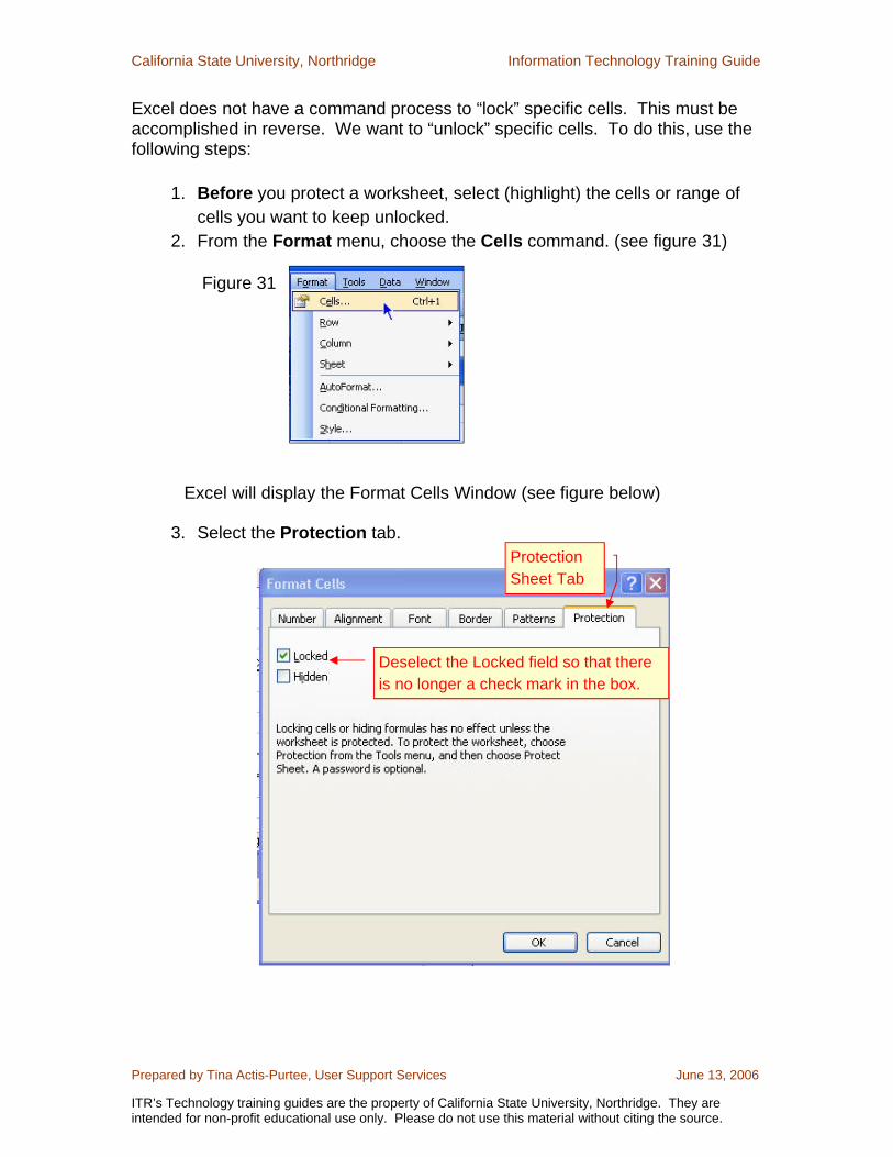
Excel does not have a command process to “lock” specific cells. This must be accomplished in reverse. We want to “unlock” specific cells. To do this, use the following steps:

1. Before you protect a worksheet, select (highlight) the cells or range of cells you want to keep unlocked.

2. From the Format menu, choose the Cells command. (see figure 31)

Figure 31

Excel will display the Format Cells Window (see figure below)

3. Select the Protection tab.

Protection Sheet Tab

Deselect the Locked field so that there is no longer a check mark in the box.




4. Click on the Locked check box to deselect it. 5. Click OK

Excel does not provide any on-screen indication of the protection status of individual cells. To distinguish unlocked cells from the protected cells in the worksheet, change their format; for example, you can change cell color or add borders.

Removing a Password You can remove both the access and write reservation password from a workbook once you no longer want to protect it. To remove a password from a workbook, use the following steps:

1. Open or activate the workbook 2. Click on the File menu and click on Save As.

Excel displays the Save As dialog box.

3. Click on Tools, then General Options from the sub menu Excel displays the Save Options dialog box.

4. Select the password characters in the Password to open or Password to modify boxes.

5. Press the Delete key. 6. Click on OK.

Excel returns you to the Save As dialog box.

7. Click on Save. Excel will ask you if you want to replace the existing file.

8. Click on Yes. Excel will save the file and remove the password protection.

Documents

California State University, Northridge Information ...csunitr/guides/excel/2003/excel_wkgmulti.pdfCalifornia State University, Northridge Information Technology Training Guide Prepared