CALIBRAZIONE ED EQUALIZZAZIONE DIGITALE DELLA … · Rivista Italiana di Acustica Vol. 38 , N. 1, p. 45 Fig. 3 ... Calibrazione ed equalizzazione digitale della sonda intensimetrica

Rivista Italiana di Acustica

Vol. 38, N. 1, pp. 42-54

ISSN: 2385-2615

www.acustica-aia.it

© Associazione Italiana di Acustica, 2014

CALIBRAZIONE ED EQUALIZZAZIONE DIGITALE DELLA SONDA INTENSIMETRICA MICROFLOWN ®

CALIBRATION AND DIGITAL EQUALIZATION OF THE INTENSIMETRIC PROBE MICROFLOWN ®

Mirco Celin (1) *, Davide Bonsi (2), Antonino Di Bella (1)

1) Dipartimento di Ingegneria Industriale - Università degli Studi di Padova 2) Fondazione Scuola di San Giorgio

* Indirizzo dell’autore di riferimento - Corresponding author’s address: Via Venezia 1 - 35131, Padova, Italia e-mail: [email protected]

(Ricevuto il 29/05/2014, accettato il 11/06/2014)

RIASSUNTO

La sonda Microflown è dotata di un microfono e 3 sensori di velocità. Per calibrarli, si gene-ra un campo acustico con proprietà note, deducendo la loro sensibilità dalla risposta del micro-fono di riferimento. Per la regione di bassa frequenza, è nota la relazione tra pressione all’interno della sorgente sferica e velocità delle particelle di fronte all’altoparlante; da questa si ricava la velocità ad una certa distanza dalla sfera. Si sono quindi calcolati i filtri digitali per correggere le risposte dei sensori: la loro somma con la fase relativa è stata equalizzata con un filtro passa-tutto. Il sistema di equalizzazione presenta un’accuratezza di 0.1 dB in ampiezza e di 5° in fase. ABSTRACT

The Microflown probe is equipped with a microphone and 3 velocity sensors. To calibrate them, it is generated an acoustic field with known properties, deducting their sensitivity from the response of the reference microphone. For low frequency range, the relationship between the pressure inside the spherical source and particles velocity in front of the speaker is known; from this, velocity is obtained at a certain distance from the sphere. Therefore the digital filters are calculated to correct the sensors’ responses: their sum with the relative phase is equalized with an all-pass filter. The equalization system has an accuracy of 0.1 dB in amplitude and 5° in phase. Parole chiave: Intensimetria; Calibrazione; Equalizzazione. Keywords: Intensity; Calibration; Equalization.

Mirco Celin et. al. Calibrazione ed equalizzazione digitale della sonda intensimetrica Microflown® Calibration and digital equalization of the intensimetric probe Microflown ®

Rivista Italiana di Acustica Vol. 38, N. 1, p. 43

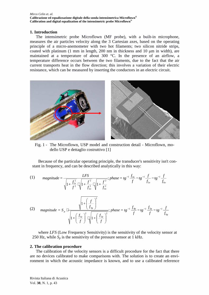
1. Introduction The intensimetric probe Microflown (MF probe), with a built-in microphone,

measures the air particles velocity along the 3 Cartesian axes, based on the operating principle of a micro-anemometer with two hot filaments; two silicon nitride strips, coated with platinum (1 mm in length, 200 nm in thickness and 10 µm in width), are maintained at a temperature of about 300 °C. In the presence of an airflow, a temperature difference occurs between the two filaments, due to the fact that the air current transports heat in the flow direction; this involves a variation of their electric resistance, which can be measured by inserting the conductors in an electric circuit.

Fig. 1 - The Microflown, USP model and construction detail - Microflown, mo-dello USP e dettaglio costruttivo [1]

Because of the particular operating principle, the transducer's sensitivity isn't con-

stant in frequency, and can be described analytically in this way:

(1) 6v5v

4v

23v

2

22v

2

2

21v

;

111f

ftg

f

ftg

f

ftg=phase

f

f+

f

f+

f

f+

LFS=magnitude 111 −−− −−

⋅⋅

(2) 6p

5p4p

2

2p

2

1p

2

3p;

11

1

f

ftg

f

ftg

f

ftg=phase

f

f+

f

f+

f

f+

S=magnitude 111p

−−− −−

⋅

⋅

where LFS (Low Frequency Sensitivity) is the sensitivity of the velocity sensor at

250 Hz, while Sp is the sensitivity of the pressure sensor at 1 kHz. 2. The calibration procedure

The calibration of the velocity sensors is a difficult procedure for the fact that there are no devices calibrated to make comparisons with. The solution is to create an envi-ronment in which the acoustic impedance is known, and to use a calibrated reference



microphone [1]. It has been performed the calibration of the red channel of the probe, corresponding to the component of the velocity vector along the y axis, dividing the procedure into two approaches: one for high frequencies and the other for low ones. The results are shown in a range between 50 Hz and 10 kHz, which is typical in sound inten-sity applications. The calibration was performed in the semi-anechoic room of the Fon-dazione Scuola di San Giorgio, with dimensions 4.7 m x 3.1 m x 2.8 m and a T30 less than 0.1 s. The equipment utilized was the same for the HF and the LF setup:

- software Adobe Audition® v3.0, for the generation and acquisition of the signals; - audio board Motu® Traveler, connected to pc via firewire bus (44.1 kHz - 16 bit); - amplifier Lab 300 Gruppen, connected to the board with a JACK/JACK wire; - sphere with loudspeaker inside, connected to the amplifier via BNC connector; - Microflown probe, USP model; - preamplifier MF, connected to the probe via LEMO 7-pin; - ½“ microphone, with a sensitivity equal to 47.6 mV/Pa, flat between 100 Hz and 10

kHz (calibrated before every measurement); - microphone preamplifier, connected to the sound level meter via LEMO 7-pin; - Sound level meter Larson Davis 831.

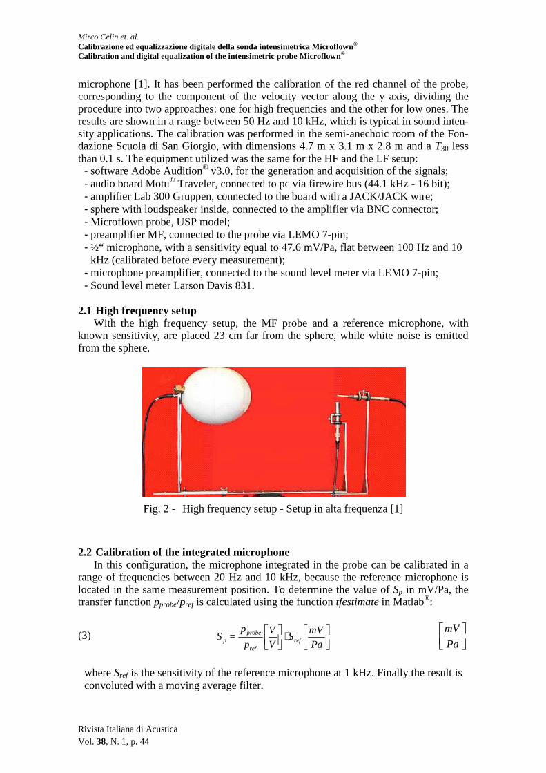
2.1 High frequency setup With the high frequency setup, the MF probe and a reference microphone, with

known sensitivity, are placed 23 cm far from the sphere, while white noise is emitted from the sphere.

Fig. 2 - High frequency setup - Setup in alta frequenza [1]

2.2 Calibration of the integrated microphone

In this configuration, the microphone integrated in the probe can be calibrated in a range of frequencies between 20 Hz and 10 kHz, because the reference microphone is located in the same measurement position. To determine the value of Sp in mV/Pa, the transfer function pprobe/pref is calculated using the function tfestimate in Matlab®:

(3)

⋅

Pa

mVS

V

V

p

p=S ref

ref

probep

Pa

mV

where Sref is the sensitivity of the reference microphone at 1 kHz. Finally the result is convoluted with a moving average filter.



Fig. 3 - Amplitude of the calibration curve for the pressure channel - Ampiezza della curva di calibrazione del canale di pressione

2.3 Calibration of the velocity sensor In order to calibrate the velocity sensor, it is necessary to utilize a spherical mono-

pole as source1, allowing to calculate the acoustic impedance of the sound field gener-ated. To obtain the sensitivity of the velocity sensor Sv, expressed in mV/Pa* 2, it has been calculated the transfer function between vprobe/pref, multiplied with the sensitivity of the reference microphone Sref and corrected with the expression of the acoustic im-pedance of the monopole Zsphere, along the axis of the loudspeaker's membrane:

(4)

⋅

⋅

Pa

mVS

Pa

PaZ

V

V

p

v=S refsphere

ref

probev

Pa

mV

(5) ( ) ( )( ) ( )

( )( ) ( )( ) ( )

( )∑

∑

−

−−

−

−

kah

krhαPαP

kah

krhαPαP

jρρ=(r)Z

'm

'm

+mm

'm

m+mm

sphere

coscos

coscos

11

11

[ ]rayl

with r = 23 cm (distance from the centre of the sphere), ρ = 1.2 kg/m3 (air density), c = 343 m/s (sound speed in air at 20°C), Pm is the Legendre function of order m, α = arcsin (b/a) with a = 9 cm (sphere radius) and b = 5 cm (loudspeaker radius), hm is the Hankel-spherical function of the second type and order m, '

mh is its derivative and k the wave number.

1 A spherical monopole is an omnidirectional source in a wide range of frequencies. This device consists of a plastic sphere, with inside a loudspeaker, and a perforated grid on the opposite side of the loudspeaker. It behaves like a sphere with a certain radius “a”, with inside a piston with a certain radius “b”, with b < a.

2 Considering that 1 Pa corresponds to 94 dBSPL, and 1 m/s (the MF operates from 10 nm/s to 1 m/s) corresponds to 146 dBSPL, it's clear that these values are hardly comparable. So it has been introduced the Pa*: 1 Pa* is the amount of velocity equivalent to 1 Pa of a plane wave without reflections, i.e. 1 Pa* = 1 Pa/ρc = 2,4 mm/s, where ρc is the acoustic impedance of the measurement environment [2].



Fig. 4 - Amplitude of the transfer function vprobe/pref (HF setup) - Ampiezza della funzione di trasferimento vprobe/pref (setup in alta frequenza)

2.4 Relative phase between the velocity and pressure channels

The cross-spectrum between velocity and pressure, that is the transfer function vprobe/pprobe, is defined as the distribution in frequency of the sound intensity; its real part corresponds to active intensity, while its imaginary part corresponds to the reactive in-tensity [3]. So the transfer function vprobe/pprobe has been calculated and multiplied with the sensitivity of the microphone of the MF probe (obtained previously) equal to 5.5 mV/Pa, and subsequently convoluted with a moving average filter. Finally it has been applied the correction for the acoustic impedance of the spherical source.

Fig. 5 - Relative phase between the velocity and the pressure channels (HF setup) - Fase relativa tra i canali di velocità e pressione (setup in alta frequenza)

Mirco Celin et. al. Calibrazione ed equalizzazione digitaleCalibration and digital equalization of the intensimetric probe Microflown


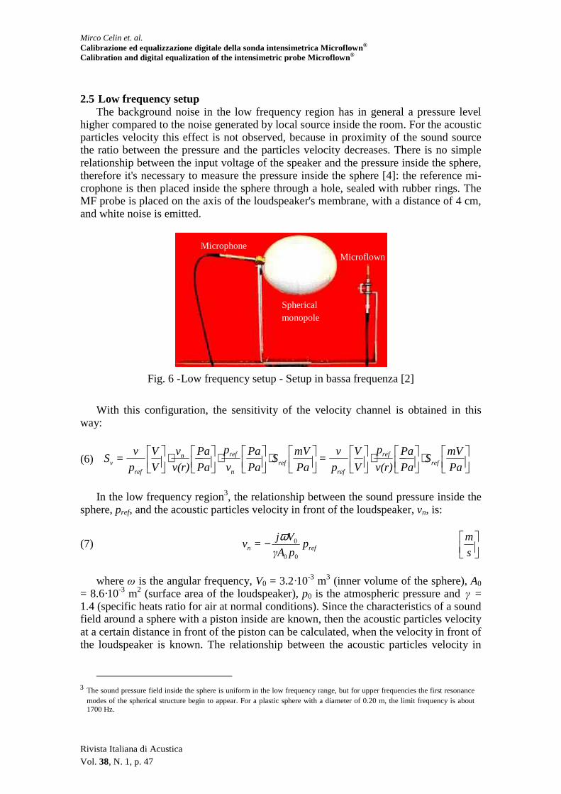
2.5 Low frequency setup

The background noise in the low frequency region has in general a pressure level higher compared to the noise generated by local source inside the room. For theparticles velocity this effect is not observed, because in proximity of the sound source the ratio between the pressure and the particles velocity decreases. There is no simple relationship between the input voltage of the speaker and the pressurtherefore it's necessary to measure the pressure inside the sphere [crophone is then placed inside the sphere through a hole, sealed with rubber rings. The MF probe is placed on the axis of the loudspeaker's membranand white noise is emitted.

Fig. 6 - Low frequency setup

With this configuration, the sensitivity of the velocity channel is obtained in this

way:

(6)

⋅

Pa

Pa

v(r)

v

V

V

p

v=S n

refv

In the low frequency region

sphere, pref, and the acoustic particles velocity in front of the loudspeaker,

(7)

where ω is the angular frequency,

= 8.6·10-3 m2 (surface area of the loudspeaker), 1.4 (specific heats ratio for air at normal conditions). Since the characteristics of a sound field around a sphere with a piston inside are known, then the acoustic particles velocity at a certain distance in front of the piston cathe loudspeaker is known. The relationship between the acoustic particles velocity in

3 The sound pressure field inside the sphere is uniform in the low frequency range, but for upper frequencies the first resonance modes of the spherical structure begin to appear.1700 Hz.

Microphone

Calibrazione ed equalizzazione digitale della sonda intensimetrica Microflown® Calibration and digital equalization of the intensimetric probe Microflown ®

The background noise in the low frequency region has in general a pressure level

higher compared to the noise generated by local source inside the room. For theparticles velocity this effect is not observed, because in proximity of the sound source the ratio between the pressure and the particles velocity decreases. There is no simple relationship between the input voltage of the speaker and the pressure inside the sphere, therefore it's necessary to measure the pressure inside the sphere [4]: the reference mcrophone is then placed inside the sphere through a hole, sealed with rubber rings. The

is placed on the axis of the loudspeaker's membrane, with a distance of 4 cm,

Low frequency setup - Setup in bassa frequenza [2]


⋅

⋅

⋅

Pa

Pa

v(r)

p

V

V

p

v=

Pa

mVS

Pa

Pa

v

p

Pa

Pa ref

refref

n

ref

In the low frequency region3, the relationship between the sound pressure inside the , and the acoustic particles velocity in front of the loudspeaker,

refn ppγA

Vj=v

00

0ω−

is the angular frequency, V0 = 3.2·10-3 m3 (inner volume of the sphere), (surface area of the loudspeaker), p0 is the atmospheric pressure and

1.4 (specific heats ratio for air at normal conditions). Since the characteristics of a sound field around a sphere with a piston inside are known, then the acoustic particles velocity at a certain distance in front of the piston can be calculated, when the velocity in front of the loudspeaker is known. The relationship between the acoustic particles velocity in

sphere is uniform in the low frequency range, but for upper frequencies the first resonance

modes of the spherical structure begin to appear. For a plastic sphere with a diameter of 0.20 m, the limit frequency is about

Microflown Microphone

Spherical monopole

The background noise in the low frequency region has in general a pressure level higher compared to the noise generated by local source inside the room. For the acoustic particles velocity this effect is not observed, because in proximity of the sound source the ratio between the pressure and the particles velocity decreases. There is no simple

e inside the sphere, ]: the reference mi-

crophone is then placed inside the sphere through a hole, sealed with rubber rings. The e, with a distance of 4 cm,

frequenza [2]


⋅

Pa

mVS

Pa

Paref

, the relationship between the sound pressure inside the , and the acoustic particles velocity in front of the loudspeaker, vn, is:

s

m

(inner volume of the sphere), A0 is the atmospheric pressure and γ =

1.4 (specific heats ratio for air at normal conditions). Since the characteristics of a sound field around a sphere with a piston inside are known, then the acoustic particles velocity

n be calculated, when the velocity in front of the loudspeaker is known. The relationship between the acoustic particles velocity in

sphere is uniform in the low frequency range, but for upper frequencies the first resonance For a plastic sphere with a diameter of 0.20 m, the limit frequency is about



front of the speaker, vn, and the particle velocity at a distance r from the centre of the sphere, is given by:

(8) ( ) ( )( ) ( )( )∑

∞

− −−0

11 coscos2 =m

'm

'm

+mmn

kah

krhαPαP

v=v(r)

s

m

where r is the distance from the membrane of the speaker. Combining equations (7) and (8), the relationship between the speed of the particles

at a distance r from the centre of the sphere and the pressure of the piston can be ob-tained:

(9) ( ) ( )( ) ( )( )∑

∞

− −⋅0

1100

coscos2γγ =m

'm

'm

+mm0

ref kah

krhαPαP

p

jωω=

p

v(r)

⋅ sPa

m

Fig. 7 - Amplitude of the sensitivity of the velocity channel (LF setup) - Ampiez-za della sensibilità del canale di velocità (setup in bassa frequenza)

2.6 Connecting the high and low frequency results

Finally the amplitude curves obtained with the calibration in HF and LF are con-nected, at 270 Hz. For the amplitude of the transfer function, the calibration curve in LF is shifted, until it reaches the calibration curve in HF [5]. In order to move the calibra-tion curve, the values of some parameters have been changed, because there's a degree of uncertainty measuring their values (ρ [kg/m3], c [m/s], V0 [m

3], A0 [m2], r [m]).

The analytic model for the velocity channel of the probe is given in equation (1). The values of the model's parameters are: Sv = 68.6 mV/Pa* at 400 Hz, f1v = 235 Hz, f2v = 490 Hz, f3v = 5300 Hz. The analytic model for the pressure channel of the probe is given in equation (2). The values of the model's parameters are: Sp = 5.5 mV/Pa at 1 kHz, f1p = 30 Hz, f2p = 48 Hz, f3p = 19300 Hz.



Fig. 8 - Amplitude curve of the velocity channel; the dashed line indicates the theoretical model - Ampiezza del canale di velocità e modello teorico

3. The digital equalization

In literature [4] it can be found that the relationship between the real specific acous-tic admittance of the sound field, Ypv (calculated in the measurement position where is located the pressure-velocity probe), and the corresponding frequency response between the signals coming from the probe, Hpv_meas provides the correction to be applied for the average acoustic intensity measurements rI , along a specific direction r :

(10) { }

measpv

pvmeaspvpvr H

YS=S=I

__ReRe

2m

W

Where Spv_meas is the measured cross-spectrum between the sound pressure and

acoustic particles velocity, Spv is the corrected cross-spectrum. Therefore, the filters, Hp_eq and Hv_eq, for the equalization of the amplitude responses of the velocity and pres-sure channels, have been calculated and used in this way: (11) ( )v_eqp_eqmeas_amppvpv_amp HHS=S ⋅⋅_

Finally, it is necessary to equalize the sum of the phase of the cross-spectrum (rela-

tive phase) and the distortion in phase of the equalizing filters, because it isn't constant. Therefore, an all-pass filter has been applied to the cross-spectrum already equalized in amplitude: (12) pass-allpv_amppv HS=S ⋅

3.1 Digitization of the transfer functions

Analyzing the three factors in which the response curve of the channel speed can be divided, it can be noticed that they correspond to the cascade of a high-pass filter, and



two low-pass filters; while for the pressure channel, the three factors correspond to the cascade of two high-pass filters and an active high-pass filter.

The discretization of a transfer function defined in the analog domain, is obtained using the Modified Bilinear Transformation, through its representation in the discrete-time (Zeta Transform). Therefore the corresponding discrete system for the low-pass fil-ter is:

(13) ( )1

ev3_discret

2F2F

1

12F −

−

⋅−⋅z

+ω

ω+

z+

+ω

ω=zS

c3v

c3v

1

c3v

3v

3.2 Inverse system

The inverse system of the discrete transfer function of the low-pass filter, is defined as:

(14) ( ) ( )zS=zS

ev3_discretsev3_d_inver

1

Starting from the system Sv3_discrete, it is possible to build a minimum phase system (a

stable system) moving the zero with unitary real part, inside the circle with unitary ra-dius. Therefore the factor 1+z-1

is substituted with 11 −⋅ zh+ v3 , where it has been added the correction factor hv3 = 0.996; the filter is now defined as:

(15) ( )1

1

sev3_d_inver 12F2F

12F

−

−

⋅

⋅−

⋅zh+

z+ω

ω+

ω

+ω=zS

v3

c3v

c3v

3v

c3v

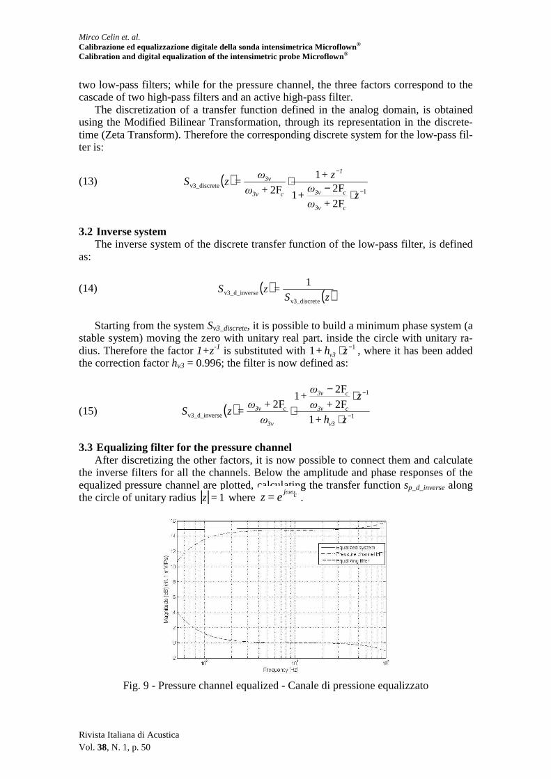
3.3 Equalizing filter for the pressure channel

After discretizing the other factors, it is now possible to connect them and calculate the inverse filters for all the channels. Below the amplitude and phase responses of the equalized pressure channel are plotted, calculating the transfer function sp_d_inverse along the circle of unitary radius | | 1=z where cjωω

e=z .

Fig. 9 - Pressure channel equalized - Canale di pressione equalizzato



3.4 Equalizing filter for the velocity channel The transfer function that describes the equalizing filter for the velocity channel is:

Fig. 10 - Velocity channel equalized - Canale di velocità equalizzato

3.5 Equalizing filter for the relative phase

The digital equalizing filters calculated contribute, in part, to the equalization of the phase responses of the probe's channels. Considering the equation (10), it can be seen that in order to correct the frequency response of the cross-spectrum, the transfer func-tions of the equalizing filters are multiplied with the measured cross-spectrum.

Fig. 11 - Relative phase corrected with digital filters - Fase relativa corretta con i filtri digitali

Then their phases are added to the relative phase obtained with the calibration pro-

cedure. From the above figure, it can be noticed that the relative phase is flat for fre-quencies above 100 Hz. In order to equalize the low frequency region, it has been ap-plied an all-pass filter, utilizing the command hdfilt.allpass in Matlab®. This is an IIR filter of the first order, with the transfer function defined as:



(16) 1pass-all 0.998011

0.99801−

−

⋅−−

z

z+=H

1

[-]

Below the relative phase, equalized with the all-pass filter, is plotted.

Fig. 12 - Relative phase, equalized with the all-pass filter - Fase relative equaliz-zata con il filtro passa-tutto

As it can be noticed from the figure, the relative phase is flat in a wide range of fre-

quencies, between -5° e 5°. 4. Developments

Recently, in the CNR (Consiglio Nazionale delle Ricerche) laboratories, it has been realized a new MEMS prototype sensible to pressure and acoustic particles velocity [6].

The chip containing the sensor has been designed with a commercial CMOS proce-dure by STMicroelectronics and has been realized with a post-processing technique. It is composed of 5 polysilicon elements on a substrate of silicon oxide. The sensor has been calibrated in the Larix laboratory of the Physics Department of the University of Ferrara, using a long impedance tube (84 m) and a progressive plane wave sound field: also in this case it is needed a known sound field in order to calibrate the prototype. The results of the calibration showed to be robust and so have been compared with the Mi-croflown’s response. Summary

The calibration of the p-v sensors remains a difficult procedure. It is compulsory to generate an acoustic signal that is high enough compared to the sound pressure caused by the background noise in the measurement point, to have a source signal linear up to 50 Hz. Analyzing the amplitude response of the pressure and velocity channels, it can be noticed the presence of a non-linearity in the curve, in a range between 4 kHz and 8 kHz, which comes to a maximum of 5 dB for the velocity. Also the relative phase is af-fected by this distortion. It has been hypothesized that the high power of the excitation signal has introduced a harmonic distortion in the response of the loudspeaker speaker in the sphere.



Another issue that has been encountered in the calibration process, is the difficulty

of accurately measuring a set of parameters, decisive for the calibration of the probe. The relationship between the particles velocity at a distance r from the centre of the

sphere, and the pressure inside the same, is used for the calibration of the transducer in LF, comparing it with the value found experimentally. This relationship depends on the precise evaluation of the surface of the loudspeaker and the volume of the sphere: inside the sphere, there are various plastic substrates (and the loudspeaker itself) that make the real volume less than that calculated from the knowledge of the radius of the sphere.

The equalizing filters provide an accurate equalization of the probe. The amplitudes of the pressure and velocity channels are perfectly equalized, with inaccuracies that ar-rive to a maximum of 0.1 dB, then negligible. The corresponding absolute phases are well compensated too. The relative phase between the two channels is well equalized thanks to the introduction of the all-pass filter. This filter does not introduce any distor-tion in amplitude within the frequency range of interest (50 Hz - 10 kHz), and as a result we obtain a flat relative phase in a range of 5°. Conclusioni

La calibrazione dei sensori MF rimane una procedura difficile. Per generare un se-gnale acustico che sia abbastanza alto rispetto al rumore di fondo nel punto di misura-zione, è obbligatorio avere un segnale sorgente lineare fino a 50 Hz. Analizzando la ri-sposta in ampiezza dei canali di pressione e velocità, si può notare la presenza di una non-linearità della curva, in un range compreso tra 4 kHz e 8 kHz, che arriva ad un mas-simo di 5 dB per la velocità. Anche la fase relativa è interessata da questa distorsione. È stato ipotizzato che l'elevata potenza del segnale di eccitazione abbia introdotto una di-storsione armonica nella risposta dell’altoparlante nella sfera. Un altro problema che è stato riscontrato nel processo di calibrazione, è la difficoltà nel misurare accuratamente una serie di parametri, decisivi per la calibrazione della sonda. Il rapporto tra la velocità di particelle ad una distanza r dal centro della sfera, e la pressione all'interno della stes-sa, viene utilizzato per la calibrazione del trasduttore in LF, confrontandolo con il valore trovato sperimentalmente. Questo rapporto dipende dalla valutazione precisa della su-perficie dell’altoparlante e il volume della sfera: all'interno di questa, ci sono vari ele-menti plastici (e l'altoparlante stesso) che rendono il volume reale inferiore a quello cal-colato dalla conoscenza del raggio della sfera. I filtri di equalizzazione forniscono una equalizzazione precisa della sonda. L'ampiezza della pressione e del canale velocità so-no perfettamente equalizzate, con imprecisioni che arrivano ad un massimo di 0.1 dB, quindi trascurabili. Anche le corrispondenti fasi assolute sono ben compensate. La fase relativa tra i due canali, è ben equalizzata grazie all'introduzione del filtro passa-tutto. Questo filtro non introduce alcuna distorsione in ampiezza nella gamma di frequenze di interesse (50 Hz - 10 kHz), e di conseguenza si ottiene un andamento della fase relativa costante in un intervallo di 5°. References [1] de Bree H.E., The Microflown, E-book, 2010.

http://www.microflown.com/library/books/the-microflown-e-book.htm (ultimo accesso: 23/05/2014)

[2] Basten T.G., de Bree H. E., Full bandwidth calibration procedure for acoustic probes containing a pressure and particle velocity sensor, The Journal of the



Acoustical Society of America, 127(1) (2010):pp. 264-270 [3] Fahy F.J., Sound intensity, Second edition, E&FN SPON, 1995 [4] Jaud V., Jacobsen F., Calibration of p-u intensity probes, in Proceedings of Euro-

noise 2006, Tampere (Finland), 30 May -1 June, 2006 [5] Raangs R., Exploring the use of Microflown, Enschede, PrintPartnersIpskamp,

2005 [6] Piotto M., Longhitano A.N., Bruschi P., Buiat M., Sacchi G., Stanzial D., Design

and fabrication of a compact p-v probe for acoustic impedance measurement, Atti del 17° Convegno Annuale AISEM, Brescia, 5-7 febbraio 2013

Documents

CALIBRAZIONE ED EQUALIZZAZIONE DIGITALE DELLA … · Rivista Italiana di Acustica Vol. 38 , N. 1, p. 45 Fig. 3 ... Calibrazione ed equalizzazione digitale della sonda intensimetrica