Calibration of effective temperature of solar type stars, using

Project report for the Master 2 Research in Astrophysics. April-June 2006

Calibration of effective temperature of solar

type stars, using equivalent width ratios of

spectral lines

Aude AlapiniUniversite Paris XI - Observatoire de Paris-Meudon

supervised byDr. Garik Israelian

Instituto de Astrofısica de Canarias, Tenerife (Canary Islands, Spain)

Instituto de Astrofısica de Canarias, C/ Va Lctea, s/n E38205 - La Laguna (Tenerife). Espana

Abstract

The effective temperature is one of the fundamental stellar parameters used to derive many quantities inastrophysics. Reducing the error bars on this variable will improve our knowledge on stellar properties.In this report, we expose an accurate calibration method for effective temperature determination of solar-type stars, using equivalent width ratios of spectral lines. We have computed a list of 250 temperaturesensitive line ratios made of 142 spectral lines from 14 different chemical elements. We have used 38 solar-type calibration stars, which temperatures have been homogeneously determined using stellar atmospheremodels. We have fitted our calibration curves using 3rd and 4th order polynomial functions.We have obtained 113 calibrations curves with small dispersion, of which 12 have very a large dynamicalrange in temperature.The accuracy of our calibration curves can still be improved using more precised equivalent width mea-surements, larger sample of calibration stars, and other type of fitting funtions. Those improvements areunder process.

La temperature effective est un des parametres stellairs fondamentaux, utilises dans de nombreusesequations en astrophysique. Diminuer les incertitudes associes a cette variable nous permettra d’ameliorernotre connaissance sur les propriets physiques des etoiles.Dans ce rapport, j’expose une methode pour calibrer la temperature effective des etoiles de type solaire.Cette methode utilise la sensibilite des rapports de largeures equivalentes de raies spectrales comme sondede temperature. Nous avons contruit 250 rapports de raies ayant une bonne sensibilite a la temperature.Ces rapports de raies sont realises a partir d’une liste de 142 raies spectral appartenant a 14 differentselements chimiques. Pour realiser cette calibration, nous avons utilise 38 etoiles de type solaire. Nousavons ajuste nos courbes de calibration a l’aide de fonctions polynomiales d’ordre 3 ou 4.113 courbes de calibrations, presentant de faibles dispersions, ont ete obtenues. Parmis celles-ci, 12presentent une bonne sensibilite sur une large plage de temperature.La precision de nos courbes de calibration peut etre amelioree en mesurant les largeures equivalentes avecplus grands soins, en utilisant davantage d’etoiles pour construire notre calibration, et en ajustant nosdonnees par d’autres type de fonctions. Ces ameliorations sont actuellement en cours.

La temperatura efectiva es uno de los parametros estelares fundamentales que usamos en muchas ecuacionesen astrofısica. Si reducimos las barras de errores en temperatura, podriamos mejorar nuestro conocimientode las propiedades estelares.En este informe, exponemos un metodo para calibrar la temperatura efectiva de las estrellas de tipo solar.Este metodo calibra la temperatura en funcion de la razon de anchuras equivalentes de las lineas espec-trales. Hemos analizado una lista de 250 razones sensibles a la variacion de temperatura, compuestas por142 lineas espectrales de 14 diferentes elementos quımicos. Disponemos de 38 estrellas de calibracion detipo solar, cuyas temperaturas han sido homogeneamente determinadas usando modelos de atmosferasestelares. Las curvas de calibracion se han ajustado usando funciones de 3ro y 4to orden.Hemos obtenido 113 curvas de calibracion con pequenas disperciones, de las cuales 12 presentan un rangode sensibilidad en temperatura bastante grande.Nuestras curvas de calibracion aun pueden ser mejoradas utilizando medidas de anchuras equivalentesmas precisas, un mayor numero de estrellas de calibracion, y otros tipos de ajustes. Estas mejorıas estanactualmente en proceso.

Acknowledgements

First of all, I would like to deeply acknowledge Garik Israelian, my supervisor on this project, for havinggiven me the opportunity of working with him in the challinging environment of the Instituto de As-trofısica de Canarias. I thank him for the diversity in the work he gave me (data reduction, analysis,observations, international conference) and for his valuable feedbacks on my report. I thank him for hiskindness and for the armenian meal he invited me to.

I would like to make special acknowledgement to Alexandra Ecuvillon. I thank her for having introducedme to Garik last summer, and for her incommensurable professional and friendly help during the project.I am grateful to her and Conrado Carretero for their disponibility (car, shopping ...) when I had my cast,and for the excursions around the Island.

I thank Gabriela Gilli for her help and comments on my report. I am grateful to Nuno Santos for thediscussions shared on the project during the Metal Rich Univers conference.I would like to thank Didier Pelat, Jacques Le Bourlot and Jacqueline Plancy from the Master 2 of As-trophysics in Paris, to have given me their agreement to carry out my Master project at the Instituto deAstrofısica de Canarias. I also thank them for providing me with the flight tickets to Tenerife.

I would like to thank a bunch of friends, without whom my stay in Tenerife won’t have been so pleasant.I am grateful to Noelia N. for her great help, especially when I had my cast, and for beeing such a kindperson. I thank, Angel L. for beeing a nice and understanding flatmate. I am grateful to Roi O. and PabloZ. for the nice times shared visiting the Island. I thank Maritza L. for beeing a understanding roommatewhen I was writting up, and for having invited me to her Tango performance (that I have unfortunatelymissed, as giving me wrong indications she sent me to the opposite side of the Island ;) ). I also thankJorge G., Sergio S., Breezy O., Kerttu V., and Santiago V. for their friendship and the nice times/chatswe shared.I am grateful to Santiago P. to have showed me how to use the software TableCurve, and to Juan M. tohave helped me with IDL. Un grand merci a Benoıt Carry pour son aide en LATEX.

I thank the secretaries of the IAC for their disponibility and patience with my Spanish. I am grateful toNicola Caon and to the computer helping desk for their help on configuring my laptop, installing softwares,and settling the videoconference.

I would like to thank Hans Deeg and Marco Montalto for the interesting discussions we had about extra-solar planetary search.

Je remercie Djibril Koudougou pour son aide aux demarches administratives francaises qu’il m’etait difficilede faire a partir de Tenerife.A special thank to Dapo Odunlade, for his understanding, patience and support.

Contents

1 Introduction 1

1.1 The interest in effective temperature measurement . . . . . . . . . . . . . . . . . . . . . . 11.2 The calibration method . . . . . . . . . . . . . . . . . . . . . . . . . . . . . . . . . . . . . 1

1.2.1 Equivalent width and line depth . . . . . . . . . . . . . . . . . . . . . . . . . . . . 21.2.2 Advantages of using line ratios . . . . . . . . . . . . . . . . . . . . . . . . . . . . . 21.2.3 Chimical abundances . . . . . . . . . . . . . . . . . . . . . . . . . . . . . . . . . . . 2

2 Selection of the line ratios 3

2.1 Line ratios . . . . . . . . . . . . . . . . . . . . . . . . . . . . . . . . . . . . . . . . . . . . . 32.1.1 Selection of the lines . . . . . . . . . . . . . . . . . . . . . . . . . . . . . . . . . . . 32.1.2 Selection of the ratios . . . . . . . . . . . . . . . . . . . . . . . . . . . . . . . . . . 42.1.3 IDl code : ratios.pro . . . . . . . . . . . . . . . . . . . . . . . . . . . . . . . . . . . 5

3 Stars and equivalent width 6

3.1 The sample of stars . . . . . . . . . . . . . . . . . . . . . . . . . . . . . . . . . . . . . . . . 63.1.1 Stellar sample already used . . . . . . . . . . . . . . . . . . . . . . . . . . . . . . . 63.1.2 More stars to be added soon . . . . . . . . . . . . . . . . . . . . . . . . . . . . . . 7

3.2 Equivalent width measurement . . . . . . . . . . . . . . . . . . . . . . . . . . . . . . . . . 83.2.1 DAOSPEC . . . . . . . . . . . . . . . . . . . . . . . . . . . . . . . . . . . . . . . . 83.2.2 DAOSPEC vs IRAF . . . . . . . . . . . . . . . . . . . . . . . . . . . . . . . . . . . 10

4 Calibration curves 11

4.1 IDL code: calibration.pro . . . . . . . . . . . . . . . . . . . . . . . . . . . . . . . . . . . . 114.2 Calibration curves and fitting function . . . . . . . . . . . . . . . . . . . . . . . . . . . . . 11

5 Futher work: improvement on the calibration curves accuracy 13

5.1 Equivalent width measurements . . . . . . . . . . . . . . . . . . . . . . . . . . . . . . . . . 135.2 Stellar sample . . . . . . . . . . . . . . . . . . . . . . . . . . . . . . . . . . . . . . . . . . . 145.3 Calibration fits . . . . . . . . . . . . . . . . . . . . . . . . . . . . . . . . . . . . . . . . . . 145.4 Apply calibration . . . . . . . . . . . . . . . . . . . . . . . . . . . . . . . . . . . . . . . . . 14

6 Conclusion 15

6.1 Conclusion on the effective temperature calibration using equivalent width ratios of spectrallines . . . . . . . . . . . . . . . . . . . . . . . . . . . . . . . . . . . . . . . . . . . . . . . . 15

6.2 General conclusion on the work experience . . . . . . . . . . . . . . . . . . . . . . . . . . . 15

7 Appendix

A Line ratios . . . . . . . . . . . . . . . . . . . . . . . . . . . . . . . . . . . . . . . . . . . . .A.1 List of spectral lines . . . . . . . . . . . . . . . . . . . . . . . . . . . . . . . . . . .A.2 List of line ratios . . . . . . . . . . . . . . . . . . . . . . . . . . . . . . . . . . . . . II

B Calibration stars . . . . . . . . . . . . . . . . . . . . . . . . . . . . . . . . . . . . . . . . . VIIC DAOSPEC input files . . . . . . . . . . . . . . . . . . . . . . . . . . . . . . . . . . . . . . VIII

C.1 daospec.opt . . . . . . . . . . . . . . . . . . . . . . . . . . . . . . . . . . . . . . . . VIIIC.2 Truncated laboratory.dat file . . . . . . . . . . . . . . . . . . . . . . . . . . . . . . VIIIC.3 Batch processing . . . . . . . . . . . . . . . . . . . . . . . . . . . . . . . . . . . . . X

D The calibration plots . . . . . . . . . . . . . . . . . . . . . . . . . . . . . . . . . . . . . . . XI

3

CONTENTS

D.1 The plots . . . . . . . . . . . . . . . . . . . . . . . . . . . . . . . . . . . . . . . . . XID.2 3rd order polynomial fitting function . . . . . . . . . . . . . . . . . . . . . . . . . . XII

E IDL programs . . . . . . . . . . . . . . . . . . . . . . . . . . . . . . . . . . . . . . . . . . . XIIIE.1 Ratios.pro . . . . . . . . . . . . . . . . . . . . . . . . . . . . . . . . . . . . . . . . . XIIIE.2 Calibration.pro . . . . . . . . . . . . . . . . . . . . . . . . . . . . . . . . . . . . . . XIX

F Notes taken on the data reduction using the ESO MIDAS UVES package . . . . . . . . . XXIII

April-June 2006 4

Chapter 1

Introduction

This report is about calibration of effective temperature using equivalent width line ratios. Before ex-plaining the method used, lets settle down the subject and have a look at why this work is of any interest.

1.1 The interest in effective temperature measurement

The effective temperature is one of the fundamental basic stellar parameters and is used in many equationsin astrophysics.

As errors propagate in the equations, decreasing the error on effective temperature can improve signifi-cantly the precision on other astrophysical parameters, like for abundances calculations for instance. Sofar, we have been dealing with temperature error bars of around 50 K, down to 20 K in some cases (Santos2004,2006, Gray 1989). Now, we are trying to decrease those errors even more, down to 10 K.

There are numerous way to derive the effective temperature of a star. One can achieve it using spectro-scopic or photometric data.The method investigated in this report uses spectral line ratios as a probe of temperature. This methodhas already been used by many authors, such as D. Gray (1994), V. Kovtyukh et al. (2003), B. Caccin etal. (2002), K. Biazzo et al. (2004).The calibration method using line ratios has been found to be quite efficient on temperature variationsmeasurements. In this method one of the main difficulties is to determine the zero point (i.e the origin ofthe line ratio axis). For F,G,K stars, the sun is an excellent calibrator to determine the zero point. Butit is not valid to calibrate effective temperature of giant stars for instance.Moreover, the temperature calibration is not valid for extrapolation. The derived calibration curves shouldonly be applied to stars of the same type as the calibrators: F,G,K stars in this report.

1.2 The calibration method

The calibration method discribed in this report uses equivalent width line ratios. The particularity of thisproject is to compute temperature with better precision, using a wide number of ratios as well as highquality spectra (high signal to noise ratio and high resolution) from an homegeneous stellar sample.

This calibration method improves the temperature measurement by providing several independent mea-surements of the effective temperature, using the same data set. Indeed, measuring a quantity N timeswill reduce the average error by a factor

√N . For instance, when using 50 calibration curves to derive

the effective temperature, one reduces the error by a factor 7, i.e if the initial error was 50 K, the finalerror would be 7 K.Measuring the temperature using different line ratios is also a way to check the consistency and theuniqueness of the calibration set. This is a way to test the non dependence of the derived temperaturewith regards to the chimicak elements or the spectral range used in the ratios.

1

CHAPTER 1. INTRODUCTION

1.2.1 Equivalent width and line depth

In the previous work investigating calibration of effective temperature, the authors have used line depthratios to probe temperature variations. In this report, we are using equivalent width ratios.

The line depth is the depth of the spectral line. To measure the line depth, different method were used :the old method was to use a simple ruler (Gray and Johanson 1991), the modern one is to use gaussianfittings (Kovtyukh et al. 2003). The height of the gaussian is the measure of the line depth. The onlyrequirement is to use high resolution spectra, as one seeks high precisions to determe the minimum of thespectral line.

The equivalent width is the area (in mA) of the spectral line. The main advantage of using equivalentwidth is to be able to measure it even using low resolution spectra. One disadvantage is that equivalentwidth measurement is more affected by the continuum uncertainty. Indeed the equivalent width is anintegral over range of wavelength, which means that it also sums the continuum uncertainty over thisrange, wherase the line depth is affected only on one unit of wavelength. For this reason, stronger lineshave larger uncertainty on their equivalent width measurement. Another disadvantage of using equivalentwitdh appears when dealing with blended lines as additional uncertainties are introduced.

The reason why line depth have been prefered to equivalent witdh is mainly because of blended lines.Indeed, when a line is blended, even when the cores are unblended, it is difficult to separate the thecontribution of its equivalent width from the one of the other line(s). Therefore, we introduce new errorsin our equivalent width measurement. When dealing with line depth, only the cores of the lines need tobe unblended.

Nevertheless, above all, the big advantage of using equivalent widths instead of line depths, is the possi-bility of measuring equivalent widths in an automated manner, using various softwares (in this project:DAOSPEC). This is a substancial gain of time, which allows work on larger star sample and on moreratios at the same time. Thus, even if we lose precision on individual temperature estimations, we improvethe quality of our calibration by multiplying the measurements.

1.2.2 Advantages of using line ratios

As in a given spectrum, spectral lines are similarly shaped by rotational and microturbulence broadening,and by spectral resolution and interstellar reddening, those effects cancel out when using line ratios (Gray1991, Kovtyukh 2003). Thus, line ratios are not sensitive to those kind of astrophysical or instrumentalline distortions.Equivalent width ratios are also independent on chimical compositions, i.e on line strengths, as long as thetwo lines are from chimical elements showing similar abundance behaviours with regards to metallicity.We have been considering this metallicity dependance when building our line ratios, as we will see in thefollowing chapter.

1.2.3 Chimical abundances

The abundance in a given chimical element X, noted [X/H], represents the abundance of the element incomparison with the abundance of hydrogen H in the object of study. This quantity can be calculate asfollowed :

[X/H ] = log (NX/NH)⋆ − log (NX/NH)⊙ (1.1)

where N is the number (in unit volume) of atoms, * is the star of study, and ⊙ is the sun.

April-June 2006 2

Chapter 2

Selection of the line ratios

The project can be divided into 3 main steps : selecting the spectral lines and building the ratios, mea-suring the equivalent widths, and combining the two to build the calibration curves.

The effective temperature calibration is realised using plots of effective temperature against line ratios.The effective temperature of the calibration stars come from an homogeneous sample derived by Santoset al. (2004,2005). We had to first build the ratios and then apply them to our first sample of 38 stars.To build the ratios, we had to find the appropriate lines and the suitable combination of lines. This is animportant step, explained in the next section. Then, we had to mesure the equivalent width of each ofthose lines for each of the stars of the sample. This is a quite tedious work to be done manualy, so we useda software called DAOSPEC which measure automaticaly all the equivalent width of the line list givenin input. The next step was to compute de ratios with those measurements and to plot the calibrationgraphs. The last step was to find the suitable function to fit those plots.

2.1 Line ratios

2.1.1 Selection of the lines

The first step of my work was to select the lines we will used to build the ratios.

The lines were taken from a list composed of 148 spectral lines provided by V. Kovtyukh, 39 FeI linesused by N. Santos to compute stellar atmosphere parameters (Nuno 2004), and 80 lines used by G. Gillito compute stellar abundances (Gilli 2006). All thoses lines are located between 5200 and 6800 A, haveexcitation potentials between 0.8 and 5.9 eV, and are in spectral regions far from telluric absorption.

We have chosen to work with wavelengths between 5200 and 6800 A for two reasons, a naive one and apratical one. This study is our first steps in building line ratios for temperature calibration, and to startsomewhere we started with Kovtyukh’s range in wavelength. This was the naive reason. The practicleone is because we have a wide sample of stellar spectra covering this range of wavelengths.

The first creteria we wanted our lines to fullfill regarded the blendings. Indeed, as we are working withequivalent width and not line depth, we have to be carefull with blended lines. We choosed to keep onlythe unblended or well blended lines. What we mean here by well blended is when the line cores areunblended, even if the line wings overlap. We have annotated the well blended lines to allow follow up ofthe ratios involving them and check if there are any dispersion excess in this calibration plots.To know if the lines were bad, well or not blended (see example on FIG.2.1), I have had to check themmanually on the spectra of HD59686 a 4871 K and [Fe/H]=0.28 star, using the SPOLT task of IRAF1.As the blending is meant to be worse in cool metal rich stars, this test tells us about how much blendedthoses lines can be in our sample. Of course, this is only to be taken as an indicator, as higher resolutionspectra can reveal unidentified bad blended line, and as some lines can become blended at higher metal-licity.

1Image Reduction and Analysis Facility

3

CHAPTER 2. SELECTION OF THE LINE RATIOS

(a) The central line is bad blended (b) Unblended and ”well” blended lines

Figure 2.1: Example of bad, well and not blended lines

We have checked the equivalent width of the lines in a solar atlas, and have chosen lines with averagestrength, i.e equivalent width between 10 mA and 200 mA.The lines with equivalent width smaller than 200 mA are more suitable for our calibration as they belongsto the linear part of the curve of growth of spectral lines, and therefore, are not distorted by saturationeffects. Nevertheless, too weak lines (equivalent width lower than 10 mA) might not be found in somestars. This will affect the density of points in the calibration graph involving those lines, and thereforewill reduce the statistic of the plot.

Applying all those criteria, we ended up with a list of 142 spectral lines, of which 78 unblended lines and67 well blended lines. Thoses lines are from various chimical elements, such as VI, AlI, CaI, CoI, CrI, FeI,MgI, MnI, NaI, NiI, SI, ScII, SiI and TiI (I stands for neutral atom and II for one time ionized element).The line list resulting from this selection is appended to this report.

This line list of well or non blended lines, has been used as input to the IDL program computing the lineratios, as dicribed in the following subsection.

2.1.2 Selection of the ratios

The second step of my work was to build temperature sensitive line ratios using the lines selected asexplained in the previous subsection.Lines should not been randomly combined in ratios. For a line ratio to be a good temperature indicator,it has to fullfill some criteria listed here after.

To minimize the influance of the contiuum evaluation uncertainty on our ratios, we combined lines closedin wavelengths (Gray 1994). Indeed, the EW of lines closed in wavelength are affected the same way bythe continuum. Thus, when computing the ratio, the contribution of the continuum will be canceled out.In their article Kovtykh at al. (2003) use a wavelength difference up to 70 A. They have tested thisvalue and have found only small dispersion on the calibartion curve. As a first approach, we use thesame value of wavelength difference in our calibration. Later, we will try to combine lines futher apartin wavelength (∼ 100 A), as the continuum is well fitted we should not be affected differences in continuum.

To build ratios with high temperature sensibility, we combined lines with large difference in excitationpotential. Indeed, lines of high or low excitation potential repond differently to the change in temperature.When the temperature varies the line strength of both lines do not respond the same way, leading to agreater change in the line ratio value.D. Gray and L. Johanson (1991) use excitational potential difference of the 2 to 4 eV. In our work we arefirst trying with a vlaue of 3 eV.

Each ratio is made of lines from different chimical elements. Indeed if we combine lines from the sameelement, we migth be affected by other temperature dependent effects as the electronic population of

April-June 2006 4

CHAPTER 2. SELECTION OF THE LINE RATIOS

energy levels can be interdependent.

We have also been carefull to combine elements having the same behaviour of [X/Fe] as a function of themetalicity [Fe/H].We have classified the chimical elements in 5 categories, according to the variation of their abundancewith regard to metallicity, using the graphs provided in G. Gilli et al (2004). FeI, MgI, SiI and TiI havebeen classified as constant in abundance with regards to metallicity. VI, AlI, NaI, NiI, ScII have beenclassified as constant-weak increasing in abundance with regards to metallicity. CaI has been classified asweakly decreasing, and CoI and MnI as strongly increasing in abundance with regards to metallicity.We have only combined elements with same or similar behaviour with metallicity (e.g. weak decreasewith constant, or strong increasing with weak increasing). We have avoided combination like strongincrease and weak decrease, as such ratio will be sensitive to variation in metallicity among the sample ofcalibration stars.

2.1.3 IDl code : ratios.pro

To build ratios fullfilling all the creteria discribed in the previous subsection, I have written a short pro-gram in IDL2. This program, called ratios.pro, uses as input the line list discribed two subsections above.It combines the lines following all the criteria discribed in the previous subsection, and returns threeoutput files: the list of ratios composed of well and non blended lines, the list of the lines appearing inthose ratios, and the list of ratios only made of unblended lines. During the run, it also prints out on theIDL terminal, the number of ratios fullfilling the required conditions.

The calling sequence for this program is

IDL> .r ratios.pro

IDL> ratios, 70., 3., 1.5

The 70. stands for the maximum difference in wavelength (in A) between the two lines, 3. stands forthe minimun difference in excitation potential (in eV), and 1.5 is a code number to tell the program tocombine elements with same or similar abundance behaviour with regards to metallicity (if this value isset to 0.0, only the elements with same abundance behaviour will be combined). The value of those threeparameters can be changed as required.

The code of this program is appended to this report.

Using ∆λmax =70 A, ∆EPmin =3 eV and ∆behavirour = 1.5, we ended up with 250 ratios made of 103lines.However, all those ratios do not give us good calibration curves. Indeed, some have high dispersion, badsensitivity to temperature, or the spectral line(s) is(are) not found in the stellar spectra. This is what weare going to see in the following chapiter.

2Interactive Data Language

April-June 2006 5

Chapter 3

Stars and equivalent width

As shown in the previous chapiter, we have built a list of ratios with a good sensitivity to temperature,which would be interesting to use for temperature calibrations.The calibration requires to measure those line ratios on many stars. The more stars is the best, as it willimprove the precision of the calibration fit.

We have chosen to start with high resolution and high signal to noise spectra. Indeed, the goodness ofthe equivalent widths measurement depends on how well the blended lines can be separated, and on howwell the noise contribution can be evaluated. In a high signal to noise spectra, the noise contribution tothe continuum is less important, making the continuum determination more accurate. High resolution ina spectra will decrease the effect of the blend, as each line will be thiner.

3.1 The sample of stars

For the calibation we are using solar type stars with a temperature range of 4500 to 6500 K (F,G,K spec-tral type stars). Most of the stars used for the calibration are metal rich stars (see the star list appendedto this report), i.e. they have metallicity greater than the solar metallicity. The spectral lines of metalrich stars are stronger, making easier their detection in the spectra.The effective temperature of those stars have been taken from the 201 stellar sample of N. Santos etal.(2004, 2005), who have computed homogeneously the stellar parameters, among which the effectivetemperature, of those stars using stellar atmosphere models. The errors on those temperatures are of theorder of 19 to 135mA.

We started by using only UVES1 spectra because of the high resolution and the high signal to noise ratioof this spectrograph. UVES is a high resolution (up to 110000 in the red) optical spectrograph, mountedon the VLT2 at La Silla in Chile. The VLT is a 8.2 m diameter telescope belonging to the ESO3 community.

An echelle spectrograph takes multiple order spectra, allowing a wider coverage in wavelength. Duringthe data reduction, the orders are extracted and combined into a single aperture spectrum.

3.1.1 Stellar sample already used

The calibration plots showed in this report are composed of 38 stars. Their spectra have been taken withUVES in 2004 (27 stars) and in 2001 (11 stars). The signal to noise ratios are of the order of 300 at lowerwavelength and 800 at higher wavelength.

The star list is appended to this report.

1Ultraviolet and Visible Echelle Spectrograph2Very Large Telescope3Europeen Southern Observatory

6

CHAPTER 3. STARS AND EQUIVALENT WIDTH

Those two series of spectra had already been reduced using a MIDAS4 pipeline for UVES data for thespectra of 2004, and using IRAF for the spectra of 2001.The spectra of 2001 appered as multiple aperture spectra. They have been combined in single aperturespectra using the SCOMBINE task of the noao.onedspec package of IRAF.

Lets explain briefly a problem encountered on the quality of the spectra used for the calibration. Wehad a star (HD102117) which spectra was harbouring strong fringing features starting around the Hα

line (6563 A). This star presented a great dispersion on the calibration graphs, i.e the ratios calculatedfor this star were wrong. We could not correct it as explain in the following, and we had to remove thisobject from our list of stars.

(a) Spectrum with fringes (b) Spectrum without fringes

Figure 3.1: Example of spectrum harbouring fringes

Fringes are due to interferences in the CCD. Why and when they occur is not yet well understood andabove all they are quite difficult to correct.So far, one way found to remove them is to use a fast rotating star. Indeed, this kind of stars have spectrawith wide spectral lines. As the fringes are high frequency features, they will be easy to distinguish inthis type of spectra. Fitting them and removing this fit from the data spectra can be a way to get ridof fringes. Nevetheless, this is not always obvious to achieve, and needs to identify a fast rotator visibleduring the obervation run. A. Ecuvillon and G. Israelian have tested this method.Another way is to identified the spectra affected by fringes and to remove them before combining thedifferent exposures. I have tested the spectrum with the selected exposure spectra, and there was noobvious improvement on the position of the star in the temperature versus ratio graphs. We think thiscan be because, to partially get rid of the fringes, we have combined only the less fringed spectra. Lessexposure time means higher signal to noise ratio. Here comes another remark : the highest is the signalto noise ratio, the most difficult it is for DOASPEC to identify correctly the spectral lines. Indeed,DAOSPEC can mistake some noise features for lines.Thus, when a spectrum turns out to harbour fringes, trying to remove them is a lot of unrewarding work.This easiest way is to remove them from the calibration.

3.1.2 More stars to be added soon

We have 14 more stars with UVES spectra, taken in service mode in 2005. They are well suitable for thefirst calibration, using only high resolution and high signal to noise spectra.

An other stage of my work was to reduced those data, using a modified version of the UVES pipeline ofthe package ESO MIDAS UVES. This version allows use a better control on the background fitting andon the cosmic ray filtering. There was 252 spectra in red to reduce. Each of them have been splited intwo: the red low part and the red up range. Each of those parts had to be reducted separatly, timing by

4Multivariate Interactive Data Analysis System

April-June 2006 7


two the number of spectra to reduce.

Those stars have not yet been added in the calibration graphs appended to this report. Before measuringthe equivalent width of the lines for those 14 stars, their spectra first need to be individualy correctedfrom radial velocity shifts (using the DOPCOR task of the onedspec package of IRAF), and combinedstar by star.Combining many spectra of the same object increases the signal intensity without increasing the signal tonoise ratio (as the noise has no spectral coherence). It is, therefore, more interessting to take many shortexposures of the same object, even if it slows down the reduction process.

(a) Unreduced image of echelle spectrometer (b) Reduced and aperture combined spectrum

Figure 3.2: Example of reduced spectrum

3.2 Equivalent width measurement

To measure automatically the equivalent width of each line of our line list, for each star of our star list,we use a software called DAOSPEC.

3.2.1 DAOSPEC

DAOSPEC is a FORTRAN program written by P.B. Stetson at the Dominion Astrophysical Observatory(DAO) in Canada.It detects spectral lines in a spectrum and measure their equivalent width in an automatic manner.It needs, in input, the spectrum (or many spectra from the same spectrograph) and two other files:daospec.opt and laboratory.dat.

The file daospec.opt contains the configuration parameters to run DAOSPEC. Those values can always bechanged when DAOSPEC is running. However, the changes won’t be saved and will be lost when closingthe DAOSPEC session.There are 16 differents configuration parameters :

1. or: the order of the continuum fitting has been set to 6. The largest is this value, the slowest willDAOSPEC run.

2. fw: the FWHM5 is set to an intial estimate of the resolution of the spectrum(in unit of pixel).We used FWHM of 8 to 11, depending on the range in wavelength of the spectra. During its runDAOSPEC will addapt this parameter to the spectra. The closest is the first guess to the real valueof FWHM, the fastest will be DAOSPEC.

5Full Width at Half Maximum

April-June 2006 8


3. sh and lo: the short and long wavelength limit of valid part of the spectrum. DAOSPEC will fit thecontinuum and measure the equivalent width of the spectral lines only on this range of wavelengths,even if it uses the whole spectra to compute the radial velocity displacement.

4. le and ri: the left and right edge of the window used to zoom on a spectral range, to monitor theprogress of DAOSPEC while it is running.

5. re: the residual core flux (in %) corresponding to the percentage of continuum flux where linessaturate. We have set this value to 10 %.

6. mi and ma: the minimum and maximum radial velocity we are expected in the star. We have setthese values to -4 and 4 respectively.

7. ve: the velocity limit (in σ), i.e. the maximum standard deviation from stellar radial velocity, beforelines are discarded. We have set this value to 3 σ.

8. fi: this parameter (fix FWHM) is set to 0 to allow DAOSPEC to readjust the FWHM value, whilecomputing. And is set to 1 to fix during the whole run the FWHM to the value defined in the feparameter. We have set it to 0.

9. cr: this parameter (creat output) is set to 1 to creat continuum and residual output fits files, andto 0 otherwise.

10. wa: this parameter (watch progress) is set to 1 to ask DAOSPEC to draw pictures in the screen.

11. sm: this parameter (smallest equivalent width in mA) is set to the minimum equivalent width for aline to be reported in the star.daospec output file. We have set it to 2.

12. sc: this parameter scales the FWHM with lambda if set to 1, and uses single FWHM if set to 0.

The other input file, laboratory.dat, contains the list of the lines that will be used to measure the radialvelocity displacement. The longest is the list, the smallest is the radial velocity displacement found byDAOSPEC in the spectrum. However, one has to be awared that the longest is the list the slowest runsDAOSPEC.

DAOSPEC can be launch on individual spectrum, or on many spectra at one time using a batch processingfile. Only spectra with the same configuration (spectograph) can be launched at the same time. This isreally useful mainly because of the gain of time in using such a procedure.

An example of doaspec.opt file is appended to this report, as well as a truncated version of the labora-tory.dat file and an example of batch processing file.

For each star, DAOSPEC produces an output file star.daospec containing the equivalent width of thespectral lines listed in the laboratory.dat file. When ”Creat DAO Spectra (cr)” is set to 1, two other filesare created: starC.fits is the .fits file of the continuum computed by DAOSPEC, and starR.fits is the .fitsfile of the residual.

DAOSPEC measures the continuum level, fits it and substracts it from the source spectra, and so onfive times. Therefore, there is no need to normalise the spectra before running DAOSPEC. In IRAF, aspectrum can be normalized using the CONTINUUM routine in the noao.onedspec package. Moreover,there is no need to correct the spectra from radial velocity shift as DAOSPEC does it using the labora-tory.dat file provided in input. In IRAF, a spectrum can be normalized using the DOPCOR task in thenoao.onedspec package.

For more details on DAOSPEC, please refer to the ”Cooking book” of DAOSPEC or visit the web pages :http://cadcwww.hia.nrc.ca/stetson/daospechttp://stars.bo.astro.it/∼GC/personal/epancino/projects/daospec.html

April-June 2006 9


(a) Overplot of a non-normalized spectrum and of its continuum fit

determinded by DAOSPEC, on the 5400-5800 A wavelength range

(b) Residual of the normalization (difference between non-normalized and normalized spectrum)

realized by DAOSPEC on the 5400-5800 A wavelength range

Figure 3.3: Illustration of the continuum fitting realized by DAOSPEC

3.2.2 DAOSPEC vs IRAF

DAOSPEC is a great gain of time when measuring the equivalent width of the spectral lines. However,as it is an automated lines search program, we needed to test its accuracy. We have compared someof DAOSPEC equivalent width measurements with manual measurements using the SPLOT routine ofIRAF. It turns out that the two methods agree within 5-10% percent errors, which is quite good consid-ering the 10% uncertainties in measuring the continuum manually.The errors on equivalent width measurements come mainly from the errors on the continuum fitting, butalso from the capacity to extract the line contribution in the case of blended lines. Therefore, to check ifDAOSPEC was dealing correctly with blended lines, we measured manually the equivalent of some wellblended lines using the deblending command of the SPOLT task of IRAF. It appears that the differencebetween the two methods was in the error range (10%) of handmade measurements using IRAF. Theerrors on equivalent width measurement when using IRAF, come also mainly from the uncertainty on thehandmade evaluation of the continuum level.

Therefore within 5-10%, DAOSPEC is able to measure correctly the equivalent width of spectral lines,including well blended lines.

DAOSPEC is known to underestimate the continuum level of around 3 mA (see the manual ”Cookingwith DAOSPEC”) in comparison with manual evaluations. In noisy spectra, this might be dued to thenormalization method used by DAOSPEC. Indeed, DAOSPEC evaluates the continuum level, detectingthe lines of the laboratory.dat file, substracting them from the spectrum, and so on five times. If thespectra is quite noisy, DAOSPEC can identify part of the noise as spectral lines and therefore substractesmore than necessary. This results in a lower estimation of the continuum level.S. Sousa et al. have worked on the comparison between DAOSPEC and IRAF, and have deduced a goodagreement between the two method, especially in the red spectral range (Sousa et al. 2006, article shouldsoon be published).

April-June 2006 10

Chapter 4

Calibration curves

All the work, discribed in the previous chapters, had been done to build calibration curves of effectivetemperature against equivalent width line ratios. On one hand, we have built temperature sensitive lineratios, and on the other hand, we have measured the equivalent width of all the lines of the ratios fora sample of 38 stars. Now, lets see how we can combine the two to derive the effective temperaturecalibration curves.

4.1 IDL code: calibration.pro

To compute the line ratios for the 38 stars of our sample, I had to write an IDL program, called calibra-tion.pro.This program has three input files: the list of stars with their temperature, the list of DAOSPEC outputfile of each star (starname.daospec) containing all the equivalent width measurements, and the list of lineratios. It gives in output the calibration graphs of temperature vs ratio for each ratio with oveplotted 4th,5th and 6th order polynomial fit. For each ratio, the best fit, i.e with the minimum standard deviation,will be the temperature calibration curve of this ratio.

The calling sequence for this program is

IDL> .r calibration.pro

IDL> calib

The code of this program is appended to this report.

4.2 Calibration curves and fitting function

Several type of calibration curves are encountered among the 250 effective temperature versus line ratiographs.There are cases where at least one of the line of the ratio has not been found. When this occurs, theconcerned stars are plotted with an equivalent width ratio of zero. There are other cases when no maintrend of the temperature as a function of the ratio, stands out. We do not really know yet why someof the calibration graphs do not have a well defined relation between temperature and line ratio, whilesome others do. This could be caused by errors in the equivalent width measurement, for example whenone line has not been identified correctly by DAOSPEC. This is something we are trying to improve asdiscussed in the following section. Those two first types of graphs are not of scientifical interest.The third category is when the variation in temperature is well defined as a function of the line ratio.Those graphs have been fitted using a polynomial function of the 3rd and 4th order. The 12 best (smalldispersion, good dynamics) calibration graphs, with the fits superimposed, can be find appended to thisreport.

The fitting function used so far are very basic, and sometimes do not reflect correctly the tendancy of theobserving effective temperature versus equivalent width line ratio. There are other simple functions onecan use to fit the calibration, such as logaritmic, exponential or power law function, as will be seen in the

11

CHAPTER 4. CALIBRATION CURVES

following section.

For 117 line ratios, one or the two spectral lines were not found. All the stars then have a line ratio valueof zero. Those graphs cannot be used for calibration.Among the 133 remaining line ratios, 113 have well defined trend of temperature with equivalent widthline ratio.And among those 113, 12 have very small dispersion and have a very good sensitivity to temperature, i.edo not flatten in temperature at high value of the line ratio, or do not tend towards infinity for low valueof the line ratio. For the remaining 101 line ratios, we will try to decrease the dispersion, as described inthe following chapiter.

The 12 best calibration curves are appended to this report.

(a) Line(s) not found (b) High dispersion

(c) Low dispersion (d) Low dispersion, good dynamics

Figure 4.1: Example of the type of temperature vs ratio graphs encountered

April-June 2006 12

Chapter 5

Futher work: improvement on the

calibration curves accuracy

Best calibration can be achieved by improving the precision of the equivalent width measurement, byadding more stars to the plot, and by using more appropriate fitting function. Here after are some moredetails about those ways of improvements.

5.1 Equivalent width measurements

The calibration graphs are plots of effective temperature against equivalent width ratios. Therefore, theerrors on the calibration curves depend on the errors on effective temperature measurements and on theones of equivalent width measurements.

The errors on the temperature measurement are taken from the homogeneous stellar sample of N. Santoset al. (2004, 2005). The smallest error on effective temperature measured is 20 K but in average theerrors are of the order of 50 K.

One way to improve the precision of our calibration curve is to decrease the errors on equivalent witdhmeasurements. As discribed in S. Sousa et al. (in press, 2006), DAOSPEC gives more precise values ofthe radial velocity shift when chosing small ranges of wavelengths for the continuum fitting and the lineidentification (parameter sh and lo of DAOSPEC). Our first attempt was to use the whole spectral range.We noticed an improvement on dispersions in the calibration graphs when using equivalent width ratiosmeasured with a wavelength range of a third of the whole spectral range.We are planning to reduce this wavelength range down to 100 A, i.e to run DAOSPEC 10 times for eachstellar spectrum. This will take longer but will improve significantly the precision on the equivalent widthmeasurement. Moreover, it can be done using a batch processing file containing the list of spectra to useand their associated configuration parameters.

The laboratory.dat file, containing the line list we want DAOSPEC to identify in the stellar spectrum,should have as many lines as possible as DAOSPEC needs a lot of comparison lines to evaluate correcltythe radial velocity shift. If the radial velocity is not well measured, DAOSPEC might identifiy the linesin a wrong way, thus, inducing dispersion in our calibration graphs.We are planning to add more comparison lines in the laboratory.dat file, especially for wavelengths between5800 and 6800 A.For now, we will not add more lines in the 4800 to 5800 A range as we already have enough lines.DAOSPEC runs slower when dealing with a large input list of spectral lines. Therefore, there is a balanceto find between the number of lines to ask DAOSPEC to identify and the time we are ready to spend onthe equivalent width measurements.

13

CHAPTER 5. FUTHER WORK: IMPROVEMENT ON THE CALIBRATION CURVES ACCURACY

5.2 Stellar sample

The precision of the calibration can be immproved by adding more calibration stars.

We have to add the remaining 14 stars taken in a service mode. Those stars have effective temperaturebetween 4800 K and 6200 K.

We are also missing stars of effective temperature between 4500 K and 5500 K and above 6300 K. To fillthose gaps, we are planning to add stellar spectra from other spectrometers, weighting the importance ofusing high quality (resolution, signal to noise ratio) spectra and the importance of having a large numberof calibration stars for statistics and temperature range coverage.In our spectral data base, we have stellar spectra from the FEROS1 and the SARG2 spectrometers. Thosespectra are already reduced. We need to run DAOSPEC and add those stars in the calibration graphs.

5.3 Calibration fits

The aim of this project is to provide accurate calibration functions of effective temperature versus equiv-alent width line ratio.

So far, we have used polynomial fitting as first guess. However, logarithm, exponential or power lawfunctions may provide even better fits to the data.As each ratio has a different best fitting function and we are dealing with a large number of ratios, wedecided to use a software which gives us a wide range of possible fitting functions to the data we provide,in order of goodness of the fit. This software, called TableCurve, is Windows based and is available onthe web for free. TableCurve can return some very complicated functions and it is then up to us to chosethe best and simplest fitting function (polynomial, logarithmic, exponantial or power law). Indeed, inphysics, the simplest explaination is the best.

This investigation of the best fitting function is under process as it depends on the data provided. Thosedata are still under improvement as we need to get more accurate equivalent width measurements and tocomplete our stellar calibration sample.

5.4 Apply calibration

The first application should be on the Sun. Indeed, comparing the temperature derived from our calibra-tion with the canonical Solar temperature, will allow us to fix the zero point of our temperature calibrationscale.

Later, we will be able to use our calibration curves to measure temperature on solar-type stars. Toevaluate the accuracy of our calibration, we will first work on a small sample of stars and compare theerrors in temperature derived from our calibration curves with the ones found in the literature.

1Fiber-fed Extended Range Optical Spectrometer, on the ESO 1.52m telescope in La Silla, Chile2Spectrografe Alta Resolusions Galileo, on the Telescopio Nazional Galileo (TNG) in La Palma, Spain

April-June 2006 14

Chapter 6

Conclusion

6.1 Conclusion on the effective temperature calibration using

equivalent width ratios of spectral lines

We have selected a line list of 142 spectral lines (unblended, or blended with line cores well separated)from different chemical elements: VI, AlI, CaI, CoI, CrI, FeI, MgI, MnI, NaI, NiI, SI, ScII, SiI and TiI (Istands for neutral atom and II for one time ionized element).

Using this line list we have built 250 temperature sensitive line ratios. Each ratio is a combination oftwo lines from different chemical elements having the same abundance behaviour with metallicity. Thecombined lines are close in wavelength (seprations less than 70 A) and have a difference in excitationpotential greater than 3 eV.

As calibrators, we have used UVES spectra of 38 solar-type stars with temperature between 4700 and6400 K. We ran an automated spectral line search software, DAOSPEC, which calculates the equivalentwidths of the lines provided in an input line list.

We have computed, for each of the 38 stars, the values of the 250 line ratios. Then, for each ratio, wehave plotted a calibration graph of effective temperatures versus equivalent width ratio measurements.Finally, we have fitted those curves by 3rd and 4th order polynomial functions.As a result of this work, we have obtained 113 good calibration curves of effective temperatures versusequivalent width ratio measurements. Among those 113 curves, 12 have very high accuracy.

There are various ways to improve the accuracy of our calibration curves, such as using more precisedequivalent width measurements, larger sample of stars, and better fitting functions. Those improvementsare under process and should be carried out by the end of August 2006.

Once those improvements are done, applying our calibration curves to the Sun will fix the zero point ofour temperature calibration scale.We shall apply our calibration to solar-type stars. Using 113 spectral line ratios, we are expecting todecrease the error bars on temperature by a factor of 10.

6.2 General conclusion on the work experience

This work experience has been a great opportunity for me, professionally, technically and socially speak-ing. I have learnt and done a lot, and still have some interesting work to complete.

Professionaly speaking, I have been working at the Instituto de Astrofisica de Canarias, an internationalcenter of research in astrophysics. I have observed two nights at the Telescopio Nazionale Galileo (TNG),at the Observatorio del Roque de Los Muchachos (ORM) in La Palma (Canary Islands, Spain), using the

15

CHAPTER 6. CONCLUSION

SARG spectrometer. And, I have attended my first week of international conference ”The Metal RichUniverse” taking place in June 2006 in La Palma.

Technically speaking, I have learnt spectral data reduction and analysis. I have developped my knowledgeon IRAF tools and in IDL programming. I have learnt how to use efficiently DAOSPEC for equivalentwidth measurements, how to reduce UVES data using the ESO MIDAS UVES pipeline, how to use Table-Curve to find the best fitting functions to our calibration curves and how to observe with an automatedprofessional telescope. I have had an overview on MOOG used to derive abundances. I have improvedmy communication skills in English and learnt Spanish.

And socially speaking, I have been working with new people, met new friends, and discovered the twogreat Islands of Tenerife and of La Palma.

April-June 2006 16

Bibliography

K. Biazzo et al., Precise determination of stellar temperaures from spectroscopic dataMem. S.A.It suppl. Vol. 5, 109, 2004.

B. Caccin et al., Spectral line ratios as Teff indicators in solar-like starsA&A 386, 286-295, 2002.

G. Gilli et al., Abundances of refractory elements in the atmospheres of stars with extrasolar planetsA&A 449, 723-736, 2006.

D. Gray and H. Johanson, Precise measurement of stellar temperatures using line depth ratiosAstromical Society, 103:439-443, 1991.

D. Gray, Spectral Line-Depth Ratios as Temperature Indicators for Cool StarsAstromical Society, 106:1248-1257, 1994.

V. Kovtyukh et al., High precision effective temperature for 181 F-K dwarfs from line-depth ratiosA&A 411, 559-564, 2003.

N. Santos et al., Spectroscopic [Fe/H] for 98 extra-solar planet-host starsA&A 415, 1153-1166, 2004.

N. Santos et al., Spectroscopic metallicities for planet-host stars: Extending the samplesA&A 437, 1127-1133, 2005.

S. Sousa et al., Spectroscopic Parameters for a sample of metal-rich solar-type starsA&A in press, 2006.

E.A. Gurtovenko and R.I. Kostik, The System of solar oscillator strengths.

Chapter 7

Appendix

A Line ratios

A.1 List of spectral lines

Here after is the list of the spectral lines used in our effective temperature calibration.

Table 7.1: This table presents the list of spectral lines used in this project. The columns (1) and (2) havebeen taken for the VALD data base. The lines annotated ”bl” are well blended. The ones annotated byan asterisk are not present in the 250 line ratios computed. In column (4), the K. stands for Kovtyukh,G. for Gilli(2006) and S. for Santos(2004). Continuation of this list on the following table

λ(A) χl log gf EW⊙ Origin λ (A) χl log gf EW⊙ Origin(1) (1) (mA) (2) (3) (4) (1) (1) (mA) (2) (3) (4)

VI AlI5670.85 1.08 −0.460 16 K.G. 6696.03 3.14 −1.570 33 bl * G.5703.59 1.05 −0.211 26 K. CaI5737.07 1.06 −0.770 11 G. 5512.98 2.93 −0.440 94 * G.6039.73 1.06 −0.650 11 K. 5590.12 2.52 −0.710 86 bl * G.6090.21 1.08 −0.150 29 K.G. 5581.97 2.52 −0.650 91 * G.6081.44 1.05 −0.579 15 bl K. 6166.44 2.52 −1.120 54 * G.6111.65 1.04 −0.715 12 K. 6169.05 2.52 −0.730 85 bl * G.6135.36 1.05 −0.746 12 bl K. 6169.56 2.52 −0.440 98 bl * G.6216.35 0.28 −0.900 30 bl G. 6449.82 2.52 −0.630 98 bl * G.6243.11 0.30 −0.980 24 bl K. 6455.60 2.52 −1.370 48 * G.6251.82 0.28 −1.340 12 K.NaI5688.22 2.10 −0.625 121 bl G.6160.75 2.10 −1.316 44 G.

CHAPTER 7. APPENDIX

Table 7.2: Continuation of table 7.1

λ(A) χl log gf EW⊙ Origin λ (A) χl log gf EW⊙ Origin(1) (1) (mA) (2) (3) (4) (1) (1) (mA) (2) (3) (4)

CoI FeI5301.04 1.71 −1.930 21 bl * G. 5247.06 0.09 −4.932 76 bl * S.5342.70 4.02 0.574 29 bl * G. 5650.71 5.08 −0.960 34 bl K.5483.36 1.71 −1.220 42 bl * G. 5651.47 4.47 −2.000 16 bl K.5647.23 2.28 −1.580 11 * G. 5662.52 4.17 −0.573 92 bl K.6093.14 1.74 −2.340 11 * K.G. 5680.26 4.18 −2.580 10 bl K.6455.00 3.63 −0.280 11 * G. 5691.51 4.30 −1.520 38 bl K.CrI 5696.10 4.54 −1.720 13 bl K.5665.56 4.92 −1.980 14 bl * G. 5701.54 2.55 −2.216 86 K.5690.43 4.93 −1.790 19 bl * G. 5705.99 4.60 −0.530 74 K.6330.13 0.94 −2.920 25 K. 5731.77 4.25 −1.300 59 K.MgI 5753.12 4.26 −0.688 78 bl K.5711.09 4.34 −1.706 107 G. 5760.35 3.64 −2.490 18 bl * K.6319.24 5.10 −2.179 39 bl G. 5855.08 4.61 −1.529 23 * S.NiI G. 5862.36 4.54 −0.058 87 * K.5413.68 3.85 −0.470 24 5956.70 0.85 −4.605 60 * K.5578.72 1.67 −2.650 46 K.G. 5983.69 4.54 −1.878 68 bl K.5587.86 1.93 −2.380 49 bl G. 5987.05 4.79 −0.556 68 bl K.5682.20 4.10 −0.390 52 bl G. 6003.03 3.88 −1.120 86 bl * K.5694.99 4.09 −0.600 44 bl G. 6007.96 4.65 −0.966 59 bl K.5754.68 1.93 −2.330 73 bl K. 6027.06 4.08 −1.180 66 S.5847.00 1.68 −3.410 19 * G. 6055.99 4.73 −0.460 73 K.S.6007.31 1.67 −3.330 20 K. 6056.01 4.73 −0.498 73 bl S.6086.29 4.26 −0.440 43 K.G. 6062.89 2.17 −4.140 18 bl K.6108.12 1.67 −2.450 60 K. 6065.48 2.60 −1.530 115 K.6130.14 4.26 −0.950 23 bl G. 6078.50 4.79 −0.424 91 K.6175.42 4.08 −0.559 36 bl K. 6085.27 2.75 −3.095 40 * K.6176.81 4.08 −0.260 50 K. 6089.57 4.58 −3.112 32 K.6186.74 4.10 −0.960 22 K. 6098.28 4.55 −1.880 16 bl K.6204.64 4.08 −1.100 16 K. 6102.18 4.83 −0.627 84 bl K.6327.60 1.67 −3.150 36 K. 6127.91 4.14 −1.399 48 bl K.6586.33 1.95 −2.810 35 K. 6151.62 2.17 −3.299 41 K.S.6767.77 1.82 −2.170 83 K. 6157.73 4.07 −1.240 64 bl S.ScII 6159.38 4.61 −1.860 12 S.5239.82 1.45 −0.760 55 bl * G. 6165.37 4.14 −1.503 43 S.5318.36 1.36 −1.700 12 * G. 6188.00 3.94 −1.631 50 S.5526.82 1.77 0.150 76 G. 6200.32 2.60 −2.437 55 K.S.6245.62 1.51 −1.040 30 G. 6213.43 2.22 −2.482 61 K.SiI 6226.73 3.88 −2.066 31 bl K.S.5517.53 5.08 −2.384 14 K. 6229.23 2.84 −2.805 33 * K.S.5621.60 5.08 −2.500 11 K. 6232.65 3.65 −1.223 76 K.5645.62 4.93 −2.140 35 bl K. 6240.66 2.22 −3.233 40 bl K.S.5690.43 4.93 −1.790 53 K.G. 6246.32 3.60 −0.733 112 K.5701.11 4.93 −2.020 40 K.G. 6252.55 2.40 −1.687 109 K.5708.41 4.95 −1.470 77 bl K. 6254.26 2.27 −2.443 115 K.5753.65 5.61 −0.830 49 bl K. 6265.13 2.17 −2.550 72 bl K.S.5772.15 5.08 −1.620 47 K.G. 6270.23 2.86 −2.583 56 bl * S.6131.86 5.61 −1.140 27 bl K. 6330.86 4.73 −1.740 32 K.6142.49 5.61 −1.480 34 K.G. 6380.75 4.19 −1.321 52 bl S.6145.02 5.61 −1.480 38 bl K.G. 6392.55 2.28 −3.932 19 bl K.S.6155.14 5.61 −0.750 72 K.G. 6419.98 4.73 −0.240 80 bl * K.6243.81 5.61 −0.770 43 bl K. 6591.33 4.59 −1.975 10 bl * S.6244.48 5.61 −0.690 45 K. 6592.91 2.72 −1.473 12 bl K.6414.99 5.87 −1.100 45 bl K. 6627.56 4.54 −1.680 24 * K.S.6583.71 5.95 −1.640 15 K. 6609.12 2.55 −2.692 76 bl K.6721.85 5.86 −1.090 55 K.G. 6653.84 4.15 −2.408 12 bl * S.TiI 6677.99 2.69 −1.418 122 bl K.5490.15 1.46 −0.980 18 bl K.G. 6725.39 4.10 −2.300 17 * K.S.6091.18 2.26 −0.460 14 K.G. 6726.68 4.61 −1.053 45 * S.6126.22 1.06 −1.410 20 K.G. 6733.18 4.64 −1.429 26 * S.6258.11 1.44 −0.440 42 bl G. 6750.15 2.42 −2.621 75 K.S.6261.11 1.43 −0.490 40 K.G. 6793.26 4.07 −2.326 10 bl * K.

6806.85 2.72 −3.210 24 * K.

April-June 2006 I

CHAPTER 7. APPENDIX

A.2 List of line ratios

Among the 250 ratios computed by calibration.pro, there are three categories: the ratios suitable for thecalibration (small dispersion), the ratios with high dispersion, and the ratios where at least one of thelines has not been found by DAOSPEC.

First, here after are the ratios with small dispersions, which can be used for the temperature calibration.We will need to understand the cause of the dispersion and try to correct it to obtain more precisedcalibration curves.

Table 7.3: This table presents the 12 best ratios obtained during this project. Those ratios have smalldispersions and a large dynamical range in temperature. The ”bl” key word indicates well blended lines.∆be is the difference indicates abundance behaviour with metallicity of the chimical elements used in theratio (0.0 stands for identical behaviours, and 1.5 for similar behaviours)

ratio λ (A) λ (A) ∆λ (A) ∆EP (eV) ∆be

6 FeI 5650.71 VI 5703.59 bl - 52.88 4.034 1.515 FeI 5691.51 VI 5703.59 bl - 12.08 3.250 1.525 FeI 5731.77 VI 5703.59 28.18 3.205 1.527 FeI 5753.12 VI 5703.59 bl - 49.53 3.209 1.542 FeI 6056.01 NiI 6108.12 bl - 52.11 3.054 1.5152 NiI 5682.20 VI 5703.59 bl - 21.39 3.049 0.0155 NiI 5694.99 VI 5703.59 bl - 8.60 3.039 0.0202 SiI 5645.62 VI 5703.59 bl - 57.97 3.879 1.5204 SiI 5690.43 VI 5703.59 13.16 3.879 1.5207 SiI 5701.11 VI 5703.59 2.48 3.879 1.5212 SiI 5753.65 VI 5703.59 bl - 50.06 4.565 1.5217 SiI 6131.86 TiI 6126.22 bl - 5.64 4.549 0.0

Table 7.4: This second table of line ratios presents the 101 remaining ratios with small dispersions. Theyhave a shorter dynamical ranges, as their curves of temperature vs ratio flatten or tend rapidly towardsinfinity at high temperatures. Same comments on ”bl” and ∆be as in 7.3. Continuation of the list on thefollowing table.


3 FeI 5619.60 VI 5670.85 51.25 3.305 1.55 FeI 5650.71 VI 5670.85 bl - 20.14 4.004 1.57 FeI 5651.47 VI 5670.85 bl - 19.38 3.392 1.59 FeI 5662.52 VI 5670.85 bl - 8.33 3.097 1.510 FeI 5662.52 VI 5703.59 bl - 41.07 3.127 1.513 FeI 5680.26 VI 5737.07 bl - 56.81 3.126 1.514 FeI 5691.51 VI 5670.85 bl - 20.66 3.220 1.516 FeI 5691.51 VI 5737.07 bl - 45.56 3.241 1.517 FeI 5696.10 VI 5670.85 bl - 25.25 3.467 1.519 FeI 5696.10 VI 5737.07 bl - 40.97 3.488 1.521 FeI 5705.99 VI 5670.85 35.14 3.526 1.524 FeI 5731.77 VI 5670.85 60.92 3.175 1.526 FeI 5731.77 VI 5737.07 5.30 3.196 1.528 FeI 5753.12 VI 5737.07 bl - 16.05 3.200 1.546 FeI 6056.01 VI 6111.65 bl - 55.64 3.687 1.549 FeI 6078.50 NiI 6108.12 29.62 3.119 1.550 FeI 6078.50 TiI 6126.22 47.72 3.728 0.054 FeI 6078.50 VI 6111.65 33.15 3.752 1.556 FeI 6089.57 TiI 6126.22 36.65 3.513 0.060 FeI 6089.57 VI 6111.65 22.08 3.537 1.566 FeI 6098.28 VI 6111.65 bl - 13.37 3.515 1.5

April-June 2006 II

CHAPTER 7. APPENDIX



68 FeI 6102.18 NiI 6108.12 bl - 5.94 3.159 1.569 FeI 6102.18 TiI 6126.22 bl - 24.04 3.768 0.073 FeI 6102.18 VI 6111.65 bl - 9.47 3.792 1.575 FeI 6127.91 TiI 6126.22 bl - 1.69 3.076 0.078 FeI 6127.91 VI 6111.65 bl - 16.26 3.100 1.582 FeI 6151.62 SiI 6145.02 - bl 6.60 3.440 0.083 FeI 6151.62 SiI 6155.14 3.52 3.443 0.090 FeI 6159.38 VI 6111.65 47.73 3.567 1.593 FeI 6165.37 TiI 6126.22 39.15 3.073 0.094 FeI 6165.37 VI 6111.65 53.72 3.097 1.599 FeI 6188.00 VI 6251.82 63.82 3.653 1.5103 FeI 6200.32 SiI 6155.14 45.18 3.011 0.0110 FeI 6226.73 VI 6216.35 bl - bl 10.38 3.600 1.5112 FeI 6226.73 VI 6251.82 bl - 25.09 3.593 1.5129 FeI 6392.55 SiI 6414.99 bl - bl 22.44 3.591 0.0134 MgI 5711.09 VI 5670.85 40.24 3.265 1.5135 MgI 5711.09 VI 5703.59 7.50 3.295 1.5140 MgI 6319.24 VI 6251.82 bl - 67.42 4.821 1.5144 NaI 6160.75 SiI 6145.02 - bl 15.73 3.512 1.5145 NaI 6160.75 SiI 6155.14 5.61 3.515 1.5151 NiI 5682.20 VI 5670.85 bl - 11.35 3.019 0.0153 NiI 5682.20 VI 5737.07 bl - 54.87 3.040 0.0154 NiI 5694.99 VI 5670.85 bl - 24.14 3.009 0.0156 NiI 5694.99 VI 5737.07 bl - 42.08 3.030 0.0157 NiI 5754.68 SiI 5708.41 bl - bl 46.27 3.019 1.5160 NiI 6086.29 TiI 6126.22 39.93 3.199 1.5164 NiI 6086.29 VI 6111.65 25.36 3.223 0.0168 NiI 6108.12 SiI 6145.02 - bl 36.90 3.940 1.5169 NiI 6108.12 SiI 6155.14 47.02 3.943 1.5170 NiI 6130.14 TiI 6126.22 bl - 3.92 3.193 1.5173 NiI 6130.14 VI 6111.65 bl - 18.49 3.217 0.0180 NiI 6176.81 TiI 6126.22 50.59 3.021 1.5181 NiI 6176.81 VI 6111.65 65.16 3.045 0.0185 NiI 6186.74 TiI 6126.22 60.52 3.038 1.5187 NiI 6186.74 VI 6216.35 - bl 29.61 3.825 0.0200 SiI 5621.60 VI 5670.85 49.25 4.001 1.5201 SiI 5645.62 VI 5670.85 bl - 25.23 3.849 1.5203 SiI 5690.43 VI 5670.85 19.58 3.849 1.5205 SiI 5690.43 VI 5737.07 46.64 3.870 1.5206 SiI 5701.11 VI 5670.85 30.26 3.849 1.5208 SiI 5701.11 VI 5737.07 35.96 3.870 1.5209 SiI 5708.41 VI 5670.85 bl - 37.56 3.873 1.5210 SiI 5708.41 VI 5703.59 bl - 4.82 3.903 1.5211 SiI 5708.41 VI 5737.07 bl - 28.66 3.894 1.5213 SiI 5753.65 VI 5737.07 bl - 16.58 4.556 1.5220 SiI 6131.86 VI 6111.65 bl - 20.21 4.573 1.5229 SiI 6145.02 TiI 6126.22 bl - 18.80 4.549 0.0232 SiI 6145.02 VI 6111.65 bl - 33.37 4.573 1.5235 SiI 6155.14 TiI 6126.22 28.92 4.552 0.0237 SiI 6155.14 VI 6111.65 43.49 4.576 1.5239 SiI 6155.14 VI 6216.35 - bl 61.21 5.339 1.5245 SiI 6244.48 TiI 6258.11 - bl 13.63 4.176 0.0246 SiI 6244.48 TiI 6261.11 16.63 4.186 0.0249 SiI 6244.48 VI 6251.82 7.34 5.329 1.5

April-June 2006 III

CHAPTER 7. APPENDIX

Secondly, here after are the line ratios with high dispersions. We will need to understand what causesdoes dispersions.

Table 7.6: This table lists the line ratios with high dispersion. Same comments on ”bl” and ∆be as in 7.3.


4 FeI 5650.71 NiI 5587.86 bl - bl 62.85 3.155 1.58 FeI 5651.47 VI 5703.59 bl - 52.12 3.422 1.511 FeI 5680.26 VI 5670.85 bl - 9.41 3.105 1.512 FeI 5680.26 VI 5703.59 bl - 23.33 3.135 1.518 FeI 5696.10 VI 5703.59 bl - 7.49 3.497 1.520 FeI 5701.54 SiI 5753.65 - bl 52.11 3.057 0.022 FeI 5705.99 VI 5703.59 2.40 3.556 1.523 FeI 5705.99 VI 5737.07 31.08 3.547 1.562 FeI 6098.28 TiI 6126.22 bl - 27.94 3.491 0.080 FeI 6151.62 SiI 6131.86 - bl 19.76 3.440 0.086 FeI 6157.73 VI 6135.36 bl - bl 22.37 3.019 1.592 FeI 6159.38 VI 6216.35 - bl 56.97 4.330 1.596 FeI 6165.37 VI 6216.35 - bl 50.98 3.860 1.597 FeI 6188.00 VI 6216.35 - bl 28.35 3.660 1.598 FeI 6188.00 VI 6243.11 - bl 55.11 3.639 1.5100 FeI 6200.32 SiI 6131.86 - bl 68.46 3.008 0.0102 FeI 6200.32 SiI 6145.02 - bl 55.30 3.008 0.0105 FeI 6200.32 SiI 6244.48 44.16 3.008 0.0111 FeI 6226.73 VI 6243.11 bl - bl 16.38 3.579 1.5113 FeI 6232.65 VI 6216.35 - bl 16.30 3.374 1.5114 FeI 6232.65 VI 6243.11 - bl 10.46 3.353 1.5115 FeI 6232.65 VI 6251.82 19.17 3.367 1.5130 FeI 6592.91 SiI 6583.71 bl - 9.20 3.227 0.0131 FeI 6609.12 SiI 6583.71 bl - 25.41 3.395 0.0132 FeI 6677.99 SiI 6721.85 bl - 43.86 3.171 0.0133 FeI 6750.15 SiI 6721.85 28.30 3.439 0.0136 MgI 5711.09 VI 5737.07 25.98 3.286 1.5138 MgI 6319.24 TiI 6258.11 bl - bl 61.13 3.668 0.0139 MgI 6319.24 TiI 6261.11 bl - 58.13 3.678 0.0141 NaI 5688.22 SiI 5753.65 bl - bl 65.43 3.512 1.5142 NaI 6160.75 SiI 6131.86 - bl 28.89 3.512 1.5146 NiI 5578.72 SiI 5517.53 61.19 3.406 1.5147 NiI 5578.72 SiI 5621.60 42.88 3.406 1.5148 NiI 5578.72 SiI 5645.62 - bl 66.90 3.254 1.5149 NiI 5587.86 SiI 5621.60 bl - 33.74 3.152 1.5150 NiI 5587.86 SiI 5645.62 bl - bl 57.76 3.000 1.5158 NiI 5754.68 SiI 5753.65 bl - bl 1.03 3.681 1.5183 NiI 6176.81 VI 6216.35 - bl 39.54 3.808 0.0184 NiI 6176.81 VI 6243.11 - bl 66.30 3.787 0.0188 NiI 6186.74 VI 6243.11 - bl 56.37 3.804 0.0189 NiI 6186.74 VI 6251.82 65.08 3.818 0.0196 ScII 5526.82 SiI 5517.53 9.29 3.312 1.5199 SiI 5517.53 TiI 5490.15 - bl 27.38 3.622 0.0247 SiI 6244.48 VI 6216.35 - bl 28.13 5.336 1.5248 SiI 6244.48 VI 6243.11 - bl 1.37 5.315 1.5

And finally, here after are the ratios for which at least one of the lines has not been found by DAOSPEC.This results is line ratios of value zero. We will need to understand why DAOSPEC has not found thosespectral lines and see if it is because of blends, line strength, or for any another reason.

April-June 2006 IV

CHAPTER 7. APPENDIX

Table 7.7: This table lists the 117 line ratios we have not been able to calculate. Same comments on ”bl”and ∆be as in 7.3.


0 CrI 6330.13 FeI 6330.86 0.730 3.792 1.51 CrI 6330.13 FeI 6380.75 - bl 50.62 3.249 1.52 CrI 6330.13 MgI 6319.24 - bl 10.89 4.167 1.529 FeI 5983.69 VI 6039.73 bl - 56.04 3.485 1.530 FeI 5987.05 NiI 6007.31 bl - 20.26 3.119 1.531 FeI 5987.05 VI 6039.73 bl - 52.68 3.731 1.532 FeI 6007.96 VI 6039.73 bl - 31.77 3.588 1.533 FeI 6027.06 VI 6039.73 12.67 3.016 1.534 FeI 6027.06 VI 6081.44 - bl 54.38 3.029 1.535 FeI 6055.99 NiI 6007.31 48.68 3.057 1.536 FeI 6055.99 NiI 6108.12 52.13 3.057 1.537 FeI 6055.99 VI 6039.73 16.26 3.669 1.538 FeI 6055.99 VI 6090.21 34.22 3.652 1.539 FeI 6055.99 VI 6081.44 - bl 25.45 3.682 1.540 FeI 6055.99 VI 6111.65 55.66 3.690 1.541 FeI 6056.01 NiI 6007.31 bl - 48.70 3.054 1.543 FeI 6056.01 VI 6039.73 bl - 16.28 3.666 1.544 FeI 6056.01 VI 6090.21 bl - 34.20 3.649 1.545 FeI 6056.01 VI 6081.44 bl - bl 25.43 3.679 1.547 FeI 6062.89 SiI 6131.86 bl - bl 68.97 3.440 0.048 FeI 6065.48 SiI 6131.86 - bl 66.38 3.008 0.051 FeI 6078.50 VI 6039.73 38.77 3.731 1.552 FeI 6078.50 VI 6090.21 11.71 3.714 1.553 FeI 6078.50 VI 6081.44 - bl 2.94 3.744 1.555 FeI 6078.50 VI 6135.36 - bl 56.86 3.744 1.557 FeI 6089.57 VI 6039.73 49.84 3.516 1.558 FeI 6089.57 VI 6090.21 0.64 3.499 1.559 FeI 6089.57 VI 6081.44 - bl 8.13 3.529 1.561 FeI 6089.57 VI 6135.36 - bl 45.79 3.529 1.563 FeI 6098.28 VI 6039.73 bl - 58.55 3.494 1.564 FeI 6098.28 VI 6090.21 bl - 8.07 3.477 1.565 FeI 6098.28 VI 6081.44 bl - bl 16.84 3.507 1.567 FeI 6098.28 VI 6135.36 bl - bl 37.08 3.507 1.570 FeI 6102.18 VI 6039.73 bl - 62.45 3.771 1.571 FeI 6102.18 VI 6090.21 bl - 11.97 3.754 1.572 FeI 6102.18 VI 6081.44 bl - bl 20.74 3.784 1.574 FeI 6102.18 VI 6135.36 bl - bl 33.18 3.784 1.576 FeI 6127.91 VI 6090.21 bl - 37.70 3.062 1.577 FeI 6127.91 VI 6081.44 bl - bl 46.47 3.092 1.579 FeI 6127.91 VI 6135.36 bl - bl 7.45 3.092 1.581 FeI 6151.62 SiI 6142.49 9.13 3.443 0.084 FeI 6157.73 TiI 6126.22 bl - 31.51 3.003 0.085 FeI 6157.73 VI 6111.65 bl - 46.08 3.027 1.587 FeI 6157.73 VI 6216.35 bl - bl 58.62 3.790 1.588 FeI 6159.38 TiI 6126.22 33.16 3.543 0.089 FeI 6159.38 VI 6090.21 69.17 3.529 1.591 FeI 6159.38 VI 6135.36 - bl 24.02 3.559 1.595 FeI 6165.37 VI 6135.36 - bl 30.01 3.089 1.5101 FeI 6200.32 SiI 6142.49 57.83 3.011 0.0104 FeI 6200.32 SiI 6243.81 - bl 43.49 3.008 0.0106 FeI 6213.43 SiI 6145.02 - bl 68.41 3.393 0.0107 FeI 6213.43 SiI 6155.14 58.29 3.396 0.0108 FeI 6213.43 SiI 6243.81 - bl 30.38 3.393 0.0109 FeI 6213.43 SiI 6244.48 31.05 3.393 0.0116 FeI 6240.66 SiI 6243.81 bl - bl 3.15 3.393 0.0117 FeI 6240.66 SiI 6244.48 bl - 3.82 3.393 0.0118 FeI 6246.32 VI 6216.35 - bl 29.97 3.322 1.5119 FeI 6246.32 VI 6243.11 - bl 3.21 3.301 1.5120 FeI 6246.32 VI 6251.82 5.50 3.315 1.5121 FeI 6252.55 SiI 6243.81 - bl 8.74 3.212 0.0122 FeI 6252.55 SiI 6244.48 8.07 3.212 0.0123 FeI 6254.26 SiI 6243.81 - bl 10.45 3.337 0.0124 FeI 6254.26 SiI 6244.48 9.78 3.337 0.0125 FeI 6265.13 SiI 6243.81 bl - bl 21.32 3.440 0.0126 FeI 6265.13 SiI 6244.48 bl - 20.65 3.440 0.0

April-June 2006 V

CHAPTER 7. APPENDIX



127 FeI 6330.86 NiI 6327.60 3.26 3.057 1.5128 FeI 6330.86 TiI 6261.11 69.75 3.303 0.0137 MgI 6319.24 NiI 6327.60 bl - 8.36 3.432 1.5143 NaI 6160.75 SiI 6142.49 18.26 3.515 1.5159 NiI 5754.68 SiI 5772.15 bl - 17.47 3.147 1.5161 NiI 6086.29 VI 6039.73 46.56 3.202 0.0162 NiI 6086.29 VI 6090.21 3.92 3.185 0.0163 NiI 6086.29 VI 6081.44 - bl 4.85 3.215 0.0165 NiI 6086.29 VI 6135.36 - bl 49.07 3.215 0.0167 NiI 6108.12 SiI 6142.49 34.37 3.943 1.5171 NiI 6130.14 VI 6090.21 bl - 39.93 3.179 0.0172 NiI 6130.14 VI 6081.44 bl - bl 48.70 3.209 0.0174 NiI 6130.14 VI 6135.36 bl - bl 5.22 3.209 0.0175 NiI 6175.42 TiI 6126.22 bl - 49.20 3.022 1.5176 NiI 6175.42 VI 6111.65 bl - 63.77 3.046 0.0177 NiI 6175.42 VI 6135.36 bl - bl 40.06 3.038 0.0178 NiI 6175.42 VI 6216.35 bl - bl 40.93 3.809 0.0179 NiI 6175.42 VI 6243.11 bl - bl 67.69 3.788 0.0182 NiI 6176.81 VI 6135.36 - bl 41.45 3.037 0.0186 NiI 6186.74 VI 6135.36 - bl 51.38 3.054 0.0190 NiI 6204.64 VI 6135.36 - bl 69.28 3.037 0.0191 NiI 6204.64 VI 6216.35 - bl 11.71 3.808 0.0192 NiI 6204.64 VI 6243.11 - bl 38.47 3.787 0.0193 NiI 6204.64 VI 6251.82 47.18 3.801 0.0194 NiI 6586.33 SiI 6583.71 2.62 4.003 1.5195 NiI 6767.77 SiI 6721.85 45.92 4.037 1.5197 ScII 6245.62 SiI 6243.81 - bl 1.81 4.106 1.5198 ScII 6245.62 SiI 6244.48 1.14 4.106 1.5166 NiI 6108.12 SiI 6131.86 - bl 23.74 3.940 1.5214 SiI 5772.15 VI 5703.59 68.56 4.031 1.5215 SiI 5772.15 VI 5737.07 35.08 4.022 1.5216 SiI 6131.86 TiI 6091.18 bl - 40.68 3.349 0.0218 SiI 6131.86 VI 6090.21 bl - 41.65 4.535 1.5219 SiI 6131.86 VI 6081.44 bl - bl 50.42 4.565 1.5221 SiI 6131.86 VI 6135.36 bl - bl 3.50 4.565 1.5222 SiI 6142.49 TiI 6091.18 51.31 3.352 0.0223 SiI 6142.49 TiI 6126.22 16.27 4.552 0.0224 SiI 6142.49 VI 6090.21 52.28 4.538 1.5225 SiI 6142.49 VI 6081.44 - bl 61.05 4.568 1.5226 SiI 6142.49 VI 6111.65 30.84 4.576 1.5227 SiI 6142.49 VI 6135.36 - bl 7.13 4.568 1.5228 SiI 6145.02 TiI 6091.18 bl - 53.84 3.349 0.0230 SiI 6145.02 VI 6090.21 bl - 54.81 4.535 1.5231 SiI 6145.02 VI 6081.44 bl - bl 63.58 4.565 1.5233 SiI 6145.02 VI 6135.36 bl - bl 9.66 4.565 1.5234 SiI 6155.14 TiI 6091.18 63.96 3.352 0.0236 SiI 6155.14 VI 6090.21 64.93 4.538 1.5238 SiI 6155.14 VI 6135.36 - bl 19.78 4.568 1.5240 SiI 6243.81 TiI 6258.11 bl - bl 14.30 4.176 0.0241 SiI 6243.81 TiI 6261.11 bl - 17.30 4.186 0.0242 SiI 6243.81 VI 6216.35 bl - bl 27.46 5.336 1.5243 SiI 6243.81 VI 6243.11 bl - bl 0.70 5.315 1.5244 SiI 6243.81 VI 6251.82 bl - 8.01 5.329 1.5

April-June 2006 VI

CHAPTER 7. APPENDIX

B Calibration stars

Table 7.9: This table presents the 38 solar type stars used to build our calibration graphs. The spectraof those stars were taken in 2001 and 2004 on the UVES spectrometer of the VLT.

star Teff (K) [Fe/H] Obs. date star Teff (K) [Fe/H] Obs. date

HD142 6302± 56 0.14 ± 0.07 2004 HD73256 5518± 49 0.26 ± 0.06 2004HD1237 5536± 50 0.12 ± 0.06 2004 HD73526 5699± 49 0.27 ± 0.06 2004HD4208 5626± 32 −0.24 ± 0.04 2004 HD74156 6112± 39 0.16 ± 0.05 2004HD7570 6140± 41 0.18 ± 0.05 2001 HD75289 6143± 53 0.28 ± 0.07 2001HD17051 6252± 53 0.26 ± 0.06 2001 HD82943 6028± 19 0.29 ± 0.02 2001HD19994 6121± 33 0.19 ± 0.05 2001 HD88133 5438± 34 0.33 ± 0.05 2004HD23079 5959± 46 −0.11 ± 0.06 2004 HD99492 4810± 72 0.26 ± 0.07 2004HD28185 5656± 44 0.22 ± 0.05 2004 HD106252 5866± 36 −0.03 ± 0.05 2004HD30177 5588± 57 0.39 ± 0.06 2004 HD108147 6248± 42 0.20 ± 0.05 2001HD33636 6046± 49 −0.08 ± 0.06 2004 HD114386 4834± 77 −0.04 ± 0.07 2004HD37124 5546± 30 −0.38 ± 0.04 2004 HD114762 5884± 34 −0.25 ± 0.05 2001HD39091 5991± 27 0.10 ± 0.04 2004 HD117207 5654± 33 0.23 ± 0.05 2004HD47536 4554± 85 −0.54 ± 0.12 2004 HD120136 6339± 73 0.23 ± 0.07 2001HD50554 6026± 30 0.01 ± 0.04 2004 HD121504 6075± 40 0.16 ± 0.05 2001HD52265 6103± 52 0.25 ± 0.06 2001 HD209458 6117± 26 0.02 ± 0.03 2001HD59686 4871 ± 135 0.28 ± 0.18 2004 HD213240 5984± 33 0.17 ± 0.05 2004HD65216 5666± 31 −0.12 ± 0.04 2004 HD216435 5938± 42 0.24 ± 0.05 2004HD70642 5693± 26 0.18 ± 0.04 2004 HD216437 5887± 32 0.25 ± 0.04 2004HD72659 5995± 45 0.03 ± 0.06 2004 HD219449 4757 ± 102 0.05 ± 0.14 2004

Table 7.10: This second table presents the list of the 14 stars observed in service mode (2005) with theUVES spectrometer of the VLT. Their spectra will soon be used to complete the stellar sample in ourcalibration.

star Teff (K) [Fe/H] Obs. date

HD2039 5976 ± 51 0.32 ± 0.06 2005HD4203 5636 ± 40 0.40 ± 0.05 2005HD41004 5242 ± 57 0.16 ± 0.07 2005HD76700 5737 ± 34 0.41 ± 0.05 2005HD114729 5886 ± 36 −0.25 ± 0.05 2005HD117618 6013 ± 41 0.06 ± 0.06 2005HD128311 4835 ± 72 0.03 ± 0.07 2005HD154857 5610 ± 27 −0.23 ± 0.04 2005HD177830 4804 ± 77 0.33 ± 0.09 2005HD190228 5327 ± 35 −0.27 ± 0.06 2005HD190360 5584 ± 36 0.24 ± 0.05 2005HD208487 6141 ± 29 0.06 ± 0.04 2005HD216770 5423 ± 41 0.26 ± 0.04 2005HD330075 5017 ± 53 0.08 ± 0.06 2005

April-June 2006 VII

CHAPTER 7. APPENDIX

C DAOSPEC input files

C.1 daospec.opt

Here is an example of a daospec.opt file with the typical parameter values used. Note that the value ofparameter changes for each spectral range and for each spectrograph.//

or=6 order for continuum fitting

fw=11.0 intial estimate of the resolution of the spectrum(unit=pixel)

sh=6470 short wavelength limit of valid part of the spectrum

lo=6820 long wavelength limit of valid part of the spectrum

le=6525. left edge of the window (zoom on a spectral range, monitoring)

ri=6550. right edge of the window (zoom on a spectral range, monitoring)

re = 10 residual core flux (% of contiuum flux where lines saturate)

mi = -4 minimum radiale velocity (within, star has instantaneous geocentric rv)

ma = 4 maximum radiale velocity (within, star has instantaneous geocentric rv)

ve=3 velocity limit (max std dev from stellar rv b4 line discarded)

fi=0. fix FWHM (0 : DAO find the best FWHM, 1: FWHM fixed by user)

cr=1. create output (continuum and residuals) spectra (1: yes, 0: no)

wa=1 watch progress (1: draw picture on the monitor, 0: don’t)

sm=2 smallest equivalent width (min EW b4 line not reported)

sc=1. scale FWHM with lambda (1: yes, 0: single FWHM used)

C.2 Truncated laboratory.dat file

Here is a truncated version of the laboratory.dat file used with DAOSPEC.The structure of the line comments is important, as the comments are reported in the *.daospec outputfile, next to the corresponding line. The IDL program, calibration.pro, reads this file with a definedformat to extracte the columns of the file. Therefore, to allow a correct lecture and extraction of data,the structure of laboratory.dat should be respected.In the following, the lines with comments are the ones of our line list, used to build our line ratios. Theother lines, taken in VALD and NIST atomic database, have been added to have a uniform and densedistribution of reference lines over the wavelength range of our spectra. Indeed, as seen in the main part ofthis report, the dispersion of radial velocity found by DAOSEPC decereases when the number of referencelines in laboratory.dat increases.

Input line list for DAOSPEC

Rq on EP & log(gf)

- values taken from VALD database

Rq on bl column

- unblended line = 0

- well blended = 1

- bad blended = 2

Rq on be column : behaviour of [X/Fe] with regards to [Fe/H] (Gilli2006)

- 0.0 = [X/Fe] bw constant and weak increasing with [Fe/H]

- 1.5 = [X/Fe] constant with [Fe/H]

- 3.0 = [X/Fe] bw constant and weak decreasing with [Fe/H]

- 4.5 = [X/Fe] weak decreasing with [Fe/H]

- 8.0 = [X/Fe] strong increasing with [Fe/H]

Rq on orig column

- K. = from Kovtyukh’s lines

- G. = from Gilli(2006)’s lines

- M. = from Santos’s FeI lines

April-June 2006 VIII

CHAPTER 7. APPENDIX

Elements’ atomic number (.0 = neurtal, .1= 1 time ionized):

- VI = 23.0

- AlI = 13.0

- Ba2 = 56.1

- CaI = 20.0

- CoI = 27.0

- CrI = 24.0

- Eu2 = 63.1

- FeI = 26.0

- Fe2 = 26.1

- La2 = 57.1

- MgI = 12.0

- MnI = 25.0

- NaI = 11.0

- NiI = 28.0

- SI = 16.0

- Sc2 = 21.1

- SiI = 14.0

- TiI = 22.0

- Ti2 = 22.1

wavelgt el EP log(gf) bl be orig

(eV)

##

4807.52 23.0

4827.46 23.0

.

.

.

5626.02 23.0 1.0430 -1.240 1 0.0 K.

5670.85 23.0 1.0810 -0.420 0 0.0 K.

5703.59 23.0 1.0640 -0.650 0 0.0 K.

5737.07 23.0 1.06 -0.770 0 0.0 G.

6039.74 23.0 1.0640 -0.650 0 0.0 K.

6081.45 23.0 1.0510 -0.579 1 0.0 K.

6090.22 23.0 1.0810 -0.062 0 0.0 K.

6111.65 23.0 1.0430 -0.715 0 0.0 K.

6119.53 23.0 1.0640 -0.320 1 0.0 K.

6135.37 23.0 1.0510 -0.746 1 0.0 K.

6150.15 23.0

6199.19 23.0 0.2870 -1.300 1 0.0 K.

6216.35 23.0 0.28 -0.900 1 0.0 G.

6233.20 23.0

6243.11 23.0 0.3010 -0.980 1 0.0 K.

6251.82 23.0 0.2870 -1.340 0 0.0 K.

6285.17 23.0

6452.32 23.0

.

.

.

5512.98 20.0 2.93 -0.440 0 4.5 G.

5581.97 20.0 2.52 -0.650 0 4.5 G.

5590.12 20.0 2.52 -0.710 1 4.5 G.

5857.45 20.0

6102.72 20.0

6122.23 20.0

April-June 2006 IX

CHAPTER 7. APPENDIX

6156.03 20.0

6161.30 20.0

6162.17 20.0

6166.44 20.0 2.52 -1.120 0 4.5 G.

6169.05 20.0 2.52 -0.730 1 4.5 G.

6169.56 20.0 2.52 -0.440 1 4.5 G.

6439.08 20.0

6449.82 20.0 2.52 -0.630 1 4.5 G.

6455.60 20.0 2.52 -1.370 0 4.5 G.

.

.

.

6091.17 22.0 2.2670 -0.423 0 1.5 K.

6126.22 22.0 1.0670 -1.425 0 1.5 K.

6220.50 22.0

6258.11 22.0 1.44 -0.440 1 1.5 G.

6258.71 22.0

6261.11 22.0 1.5.43 -0.490 0 1.5 K.G.

6303.76 22.0

6312.24 22.0

.

.

.

6606.95 22.1

6680.13 22.1

C.3 Batch processing

Here is an example of batch file. The calling sequence for this batch, in a linux terminal, is ”¿ batch” andall the lines (except the ones starting by # which are comment lines) are executed.

# !/bin/csh # Tell the system where is csh

# # Comment

rm HD*.daospec # Remove previous output

daospec <<DONE>! logfile # Run DAOSPEC and save log

WA=0 # Mandatory for batch processing

HD102117REDU_COR.fits # Work on spectrum


.

.

.



DONE # End of input list for DAOSPEC

April-June 2006 X

CHAPTER 7. APPENDIX

D The calibration plots

D.1 The plots

Here after are the 12 best calibration curves we have obtained, with small dispersions and a large dynam-ical range (i.e a small variation of the ratio leads to a large variation of the temperature). The data havebeen fitted by polynomial function of the 3rd and of the 4th order. As we can see from the plots, a 3rdorder polynomial function is sufficient to fit those data.

April-June 2006 XI

CHAPTER 7. APPENDIX

D.2 3rd order polynomial fitting function

A 3rd order polynimial function has for equation:

y = C0 + C1x+ C2x2 + C3x

3 (7.1)

In our calibration curves, ”y” is the effective temperature and ”x” is the line ratio. Here after are thevalues of the 4 coefficients found for our 12 best calibration curves.

Table 7.11: This table gives the coefficients of the 3rd order polynomial functions fitting the 12 bestcalibration curves derived from our data.

ratio C0 C1 C2 C3

6 3250± 170 4690 ± 460 −2950± 401 68± 11015 2440± 270 6240 ± 730 3990± 630 920± 17025 2700± 200 4240 ± 380 −1980± 220 330 ± 4027 3430± 150 2300 ± 200 −760± 81 90± 1042 1150± 730 6780 ± 1940 −2480± 1700 130± 490152 2980± 180 4190 ± 390 −2170± 270 410 ± 60155 2900± 200 5200 ± 530 −3230± 440 730± 120202 3590± 130 4170 ± 360 −2620± 320 610 ± 90204 3530± 140 3460 ± 320 −1820± 230 350 ± 50207 3400± 140 4380 ± 370 −2790± 320 650 ± 90212 3570± 120 3280 ± 250 −1580± 165 270 ± 30217 4140± 100 3090 ± 290 −1820± 270 410 ± 70

April-June 2006 XII

CHAPTER 7. APPENDIX

E IDL programs

E.1 Ratios.pro

;*********************************************************************

;

; Build line ratios

;

;criteria :

;- closed wavelengths

;- high difference in excitation potential

;- pair of different chimical elements

;- pair of chimical elements having the same behaviour of

;[X/Fe] in function of [Fe/H]

;

;*********************************************************************

;calling sequences :

;Windows

;IDL>.r E:\Stage_IAC\IDL\pro\ratios.pro

;Linux

;IDL>.r /scratch/Stage_IAC/idl/pro/ratios.pro

;

;IDL> ratios, 70., 3., 1.5

;

;*********************************************************************

pro ratios, dlamb_max, dEP_min, dbe_max

;dLamb_max in Angstrom

;EP_min in eV

;dbe_max = 0.0 (only same behaviour),

; 1.5 (similar behaviour)

path = ’E:\Stage_IAC\IDL\IDL_aspid_07_06\’ ;path Windows

;path = ’/scratch/Stage_IAC/idl/IDL_aspid_07_06/’ ;path Linux

Infile = ’InLineList.txt’

FMT = ’F,F,F,F,I,F,A5’

;------------------------------------

;read input file (= DAOSPEC’s output)

;------------------------------------

print, " "

print, " 1. Read input file "

; Windows

readcol, path + Infile, $

wlab, el, EP, lgf, bl, be, orig, $

FORMAT=FMT, SKIPLINE=2, /SILENT

; Linux

;readcol, Infile, $

; wlab, el, EP, lgf, bl, be, orig, $

; FORMAT=FMT, SKIPLINE=2, /SILENT

print, " "

April-June 2006 XIII

CHAPTER 7. APPENDIX

;------------------------------------

;Select ratios

;------------------------------------

print, " 2. Start Select ratios"

N = n_elements(wlab)

print, "# of lines (wlab) ", N

;;;;;;;;;;;;;;;;;;;;;;;;;;;;;;;;;;;;;;;;;;;

;calcul dLamb and select dlamb < dlamb_max;

;;;;;;;;;;;;;;;;;;;;;;;;;;;;;;;;;;;;;;;;;;;

print, " 2.1. Calcul dLamb and select dlamb < dlamb_max"

wlab1_todos = 0.

wlab2_todos = 0.

EP1_todos = 0.

EP2_todos = 0.

el1_todos = 0.

el2_todos = 0.

be1_todos = 0.

be2_todos = 0.

bl1_todos = 0.

bl2_todos = 0.

for i=0, (N-1) do begin

;for i=0, 4 do begin

for j=i+1, (N-1) do begin

;for j=i+1, 4 do begin

wlab1_todos = [wlab1_todos,wlab(i)]

wlab2_todos = [wlab2_todos,wlab(j)]

EP1_todos = [EP1_todos,EP(i)]

EP2_todos = [EP2_todos,EP(j)]

el1_todos = [el1_todos,el(i)]

el2_todos = [el2_todos,el(j)]

be1_todos = [be1_todos,be(i)]

be2_todos = [be2_todos,be(j)]

bl1_todos = [bl1_todos,bl(i)]

bl2_todos = [bl2_todos,bl(j)]

endfor

endfor

wlab1_todos = wlab1_todos(1:*)

wlab2_todos = wlab2_todos(1:*)

EP1_todos = EP1_todos(1:*)

EP2_todos = EP2_todos(1:*)

el1_todos = el1_todos(1:*)

el2_todos = el2_todos(1:*)

be1_todos = be1_todos(1:*)

be2_todos = be2_todos(1:*)

bl1_todos = bl1_todos(1:*)

bl2_todos = bl2_todos(1:*)

dlamb_todos = wlab1_todos-wlab2_todos

sel_dlamb = where(abs(dlamb_todos) le dlamb_max, dimsel_dlamb)

print, "# of combi with dLamb < dLamb_max ", $

dimsel_dlamb

April-June 2006 XIV

CHAPTER 7. APPENDIX

;;;;;;;;;;;;;;;;;;;;;;;;;;;;;;;;;;;;;;;;;;;;;;;;;;;;;;;;;;;;;;;;;

;calcul dEP and select dEP > dEP_min among the dlamb < dlamb_max;

;;;;;;;;;;;;;;;;;;;;;;;;;;;;;;;;;;;;;;;;;;;;;;;;;;;;;;;;;;;;;;;;;

print, " 2.2. Calcul dEP and select dEP > dEP_min, among dlamb < dlamb_max"

N2 = dimsel_dlamb

wlab1_dlamb = wlab1_todos(sel_dlamb)

wlab2_dlamb = wlab2_todos(sel_dlamb)

dlamb_dlamb = dlamb_todos(sel_dlamb)

EP1_dlamb = EP1_todos(sel_dlamb)

EP2_dlamb = EP2_todos(sel_dlamb)

el1_dlamb = el1_todos(sel_dlamb)

el2_dlamb = el2_todos(sel_dlamb)

be1_dlamb = be1_todos(sel_dlamb)

be2_dlamb = be2_todos(sel_dlamb)

bl1_dlamb = bl1_todos(sel_dlamb)

bl2_dlamb = bl2_todos(sel_dlamb)

dEP_dlamb = EP2_dlamb-EP1_dlamb

dlamb_dlamb = wlab2_dlamb-wlab1_dlamb

sel_dEP_dlamb = where(abs(dEP_dlamb) ge dEP_min, dimsel_dEP_dlamb)

print, "# of combi with dLamb < dLamb_max & dEP > dEP_min ",$

dimsel_dEP_dlamb

;;;;;;;;;;;;;;;;;;;;;;;;;;;;;;;;;;;;;;;;;;;;;;;;;;;;;;;

;condition on elements and behaviour with metallicity ;

;;;;;;;;;;;;;;;;;;;;;;;;;;;;;;;;;;;;;;;;;;;;;;;;;;;;;;;

;............................................

; Select ratios made with different elements

;............................................

print, " 2.3. Select ratios made of different elements"

N3 = dimsel_dEP_dlamb

el1_dEP_dlamb = el1_dlamb(sel_dEP_dlamb)

el2_dEP_dlamb = el2_dlamb(sel_dEP_dlamb)

be1_dEP_dlamb = be1_dlamb(sel_dEP_dlamb)

be2_dEP_dlamb = be2_dlamb(sel_dEP_dlamb)

bl1_dEP_dlamb = bl1_dlamb(sel_dEP_dlamb)

bl2_dEP_dlamb = bl2_dlamb(sel_dEP_dlamb)

wlab1_dEP_dlamb = wlab1_dlamb(sel_dEP_dlamb)

wlab2_dEP_dlamb = wlab2_dlamb(sel_dEP_dlamb)

EP1_dEP_dlamb = EP1_dlamb(sel_dEP_dlamb)

EP2_dEP_dlamb = EP2_dlamb(sel_dEP_dlamb)

dEP_dEP_dlamb = dEP_dlamb(sel_dEP_dlamb)

dlamb_dEP_dlamb = dlamb_dlamb(sel_dEP_dlamb)

sel_el_dEP_dlamb = where(el1_dEP_dlamb ne el2_dEP_dlamb, dimsel_el_dEP_dlamb)

print, "# of combi (dLamb<dLamb_max, dEP>dEP_min & el1 ne el2)",$

dimsel_el_dEP_dlamb

;............................................

April-June 2006 XV

CHAPTER 7. APPENDIX

; Select ratios made with different elements

;............................................

print, " 2.4. Select ratios made of elements with same behaviour"

N4 = dimsel_el_dEP_dlamb

be1_el_dEP_dlamb = be1_dEP_dlamb(sel_el_dEP_dlamb)

be2_el_dEP_dlamb = be2_dEP_dlamb(sel_el_dEP_dlamb)

bl1_el_dEP_dlamb = bl1_dEP_dlamb(sel_el_dEP_dlamb)

bl2_el_dEP_dlamb = bl2_dEP_dlamb(sel_el_dEP_dlamb)

el1_el_dEP_dlamb = el1_dEP_dlamb(sel_el_dEP_dlamb)

el2_el_dEP_dlamb = el2_dEP_dlamb(sel_el_dEP_dlamb)

wlab1_el_dEP_dlamb = wlab1_dEP_dlamb(sel_el_dEP_dlamb)

wlab2_el_dEP_dlamb = wlab2_dEP_dlamb(sel_el_dEP_dlamb)

EP1_el_dEP_dlamb = EP1_dEP_dlamb(sel_el_dEP_dlamb)

EP2_el_dEP_dlamb = EP2_dEP_dlamb(sel_el_dEP_dlamb)

dEP_el_dEP_dlamb = dEP_dEP_dlamb(sel_el_dEP_dlamb)

dlamb_el_dEP_dlamb = dlamb_dEP_dlamb(sel_el_dEP_dlamb)

dbe_el_dEP_dlamb = be2_el_dEP_dlamb-be1_el_dEP_dlamb

sel_dbe_el_dEP_dlamb = where(abs(dbe_el_dEP_dlamb) le dbe_max,dimsel_dbe_el_dEP_dlamb)

print, "# of combi fulfilling conditions on dLamb, dEP, el, be",$

dimsel_dbe_el_dEP_dlamb

;;;;;;;;;;;;;;;;;;;;;;;;;;;;;;;;;;;;;;;;;;;;;;;;;;

;condition on blending ;

;;;;;;;;;;;;;;;;;;;;;;;;;;;;;;;;;;;;;;;;;;;;;;;;;;

print, " 2.5. Select ratios with unblended line"

N5 = dimsel_dbe_el_dEP_dlamb

be1_dbe_el_dEP_dlamb = be1_el_dEP_dlamb(sel_dbe_el_dEP_dlamb)

be2_dbe_el_dEP_dlamb = be2_el_dEP_dlamb(sel_dbe_el_dEP_dlamb)

bl1_dbe_el_dEP_dlamb = bl1_el_dEP_dlamb(sel_dbe_el_dEP_dlamb)

bl2_dbe_el_dEP_dlamb = bl2_el_dEP_dlamb(sel_dbe_el_dEP_dlamb)

el1_dbe_el_dEP_dlamb = el1_el_dEP_dlamb(sel_dbe_el_dEP_dlamb)

el2_dbe_el_dEP_dlamb = el2_el_dEP_dlamb(sel_dbe_el_dEP_dlamb)

wlab1_dbe_el_dEP_dlamb = wlab1_el_dEP_dlamb(sel_dbe_el_dEP_dlamb)

wlab2_dbe_el_dEP_dlamb = wlab2_el_dEP_dlamb(sel_dbe_el_dEP_dlamb)

EP1_dbe_el_dEP_dlamb = EP1_el_dEP_dlamb(sel_dbe_el_dEP_dlamb)

EP2_dbe_el_dEP_dlamb = EP2_el_dEP_dlamb(sel_dbe_el_dEP_dlamb)

sel_u_dbe_el_dEP_dlamb = where((bl1_dbe_el_dEP_dlamb+bl2_dbe_el_dEP_dlamb) eq 0.0, $

dimsel_u_dbe_el_dEP_dlamb)

print, "# of combi fulfilling dLamb, dEP, el, be, unbl ",$

dimsel_u_dbe_el_dEP_dlamb

N6 = dimsel_u_dbe_el_dEP_dlamb

el1_u_dbe_el_dEP_dlamb = el1_dbe_el_dEP_dlamb(sel_u_dbe_el_dEP_dlamb)

el2_u_dbe_el_dEP_dlamb = el2_dbe_el_dEP_dlamb(sel_u_dbe_el_dEP_dlamb)

wlab1_u_dbe_el_dEP_dlamb = wlab1_dbe_el_dEP_dlamb(sel_u_dbe_el_dEP_dlamb)

wlab2_u_dbe_el_dEP_dlamb = wlab2_dbe_el_dEP_dlamb(sel_u_dbe_el_dEP_dlamb)

bl1_u_dbe_el_dEP_dlamb = bl1_dbe_el_dEP_dlamb(sel_u_dbe_el_dEP_dlamb)

bl2_u_dbe_el_dEP_dlamb = bl2_dbe_el_dEP_dlamb(sel_u_dbe_el_dEP_dlamb)

be1_u_dbe_el_dEP_dlamb = be1_dbe_el_dEP_dlamb(sel_u_dbe_el_dEP_dlamb)

April-June 2006 XVI

CHAPTER 7. APPENDIX

be2_u_dbe_el_dEP_dlamb = be2_dbe_el_dEP_dlamb(sel_u_dbe_el_dEP_dlamb)

EP1_u_dbe_el_dEP_dlamb = EP1_dbe_el_dEP_dlamb(sel_u_dbe_el_dEP_dlamb)

EP2_u_dbe_el_dEP_dlamb = EP2_dbe_el_dEP_dlamb(sel_u_dbe_el_dEP_dlamb)

print, " "

;--------------------------------------------------

;preparing the list of the lines used in the ratios

;--------------------------------------------------

wlab_dbe_el_dEP_dlamb = wlab1_dbe_el_dEP_dlamb

el_dbe_el_dEP_dlamb = el1_dbe_el_dEP_dlamb

EP_dbe_el_dEP_dlamb = EP1_dbe_el_dEP_dlamb

bl_dbe_el_dEP_dlamb = bl1_dbe_el_dEP_dlamb

be_dbe_el_dEP_dlamb = be1_dbe_el_dEP_dlamb

for i=0, N5-1 do begin

wlab_dbe_el_dEP_dlamb = [wlab_dbe_el_dEP_dlamb,wlab2_dbe_el_dEP_dlamb(i)]

el_dbe_el_dEP_dlamb = [el_dbe_el_dEP_dlamb,el2_dbe_el_dEP_dlamb(i)]

EP_dbe_el_dEP_dlamb = [EP_dbe_el_dEP_dlamb,EP2_dbe_el_dEP_dlamb(i)]

bl_dbe_el_dEP_dlamb = [bl_dbe_el_dEP_dlamb,bl2_dbe_el_dEP_dlamb(i)]

be_dbe_el_dEP_dlamb = [be_dbe_el_dEP_dlamb,be2_dbe_el_dEP_dlamb(i)]

endfor

N_temp = n_elements(wlab_dbe_el_dEP_dlamb)

sel_temp = intarr(N_temp)

for i=0, N_temp-1 do begin

sel_temp(i)=i

endfor

wlab_dbe_el_dEP_dlamb_list = 0.

el_dbe_el_dEP_dlamb_list = 0.

EP_dbe_el_dEP_dlamb_list = 0.

bl_dbe_el_dEP_dlamb_list = 0.

be_dbe_el_dEP_dlamb_list = 0.

dimsel_temp = 1.

while dimsel_temp gt 0. do begin

wlab_dbe_el_dEP_dlamb = wlab_dbe_el_dEP_dlamb(sel_temp)

el_dbe_el_dEP_dlamb = el_dbe_el_dEP_dlamb(sel_temp)

EP_dbe_el_dEP_dlamb = EP_dbe_el_dEP_dlamb(sel_temp)

bl_dbe_el_dEP_dlamb = bl_dbe_el_dEP_dlamb(sel_temp)

be_dbe_el_dEP_dlamb = be_dbe_el_dEP_dlamb(sel_temp)

wlab_dbe_el_dEP_dlamb_list=[wlab_dbe_el_dEP_dlamb_list,wlab_dbe_el_dEP_dlamb(0)]

el_dbe_el_dEP_dlamb_list =[el_dbe_el_dEP_dlamb_list,el_dbe_el_dEP_dlamb(0)]

EP_dbe_el_dEP_dlamb_list =[EP_dbe_el_dEP_dlamb_list,EP_dbe_el_dEP_dlamb(0)]

bl_dbe_el_dEP_dlamb_list =[bl_dbe_el_dEP_dlamb_list,bl_dbe_el_dEP_dlamb(0)]

be_dbe_el_dEP_dlamb_list =[be_dbe_el_dEP_dlamb_list,be_dbe_el_dEP_dlamb(0)]

sel_temp = where(wlab_dbe_el_dEP_dlamb ne wlab_dbe_el_dEP_dlamb(0),dimsel_temp)

endwhile

wlab_dbe_el_dEP_dlamb_list = wlab_dbe_el_dEP_dlamb_list(1:*)

el_dbe_el_dEP_dlamb_list = el_dbe_el_dEP_dlamb_list(1:*)

EP_dbe_el_dEP_dlamb_list = EP_dbe_el_dEP_dlamb_list(1:*)

April-June 2006 XVII

CHAPTER 7. APPENDIX

bl_dbe_el_dEP_dlamb_list = bl_dbe_el_dEP_dlamb_list(1:*)

be_dbe_el_dEP_dlamb_list = be_dbe_el_dEP_dlamb_list(1:*)

N7 = n_elements(wlab_dbe_el_dEP_dlamb_list)

;------------------------------------

;open and write output

;------------------------------------

print, " 3. Open and write output"

; Windows

OPENW, 1, path+ ’Out\’ +’LinesInRatios.txt’

OPENW, 2, path+ ’Out\’ +’ratios17-05-06.txt’

OPENW, 3, path+ ’Out\’ +’ratios17-05-06_unbl.txt’

; Linux

;;OPENW, 1, path+ ’Out/’ +’LinesInRatios.txt’

;;OPENW, 2, path+ ’Out/’ +’ratios17-05-06.txt’

;;OPENW, 3, path+ ’Out/’ +’ratios17-05-06_unbl.txt’

;OPENW, 1, ’Out/’ +’LinesInRatios.txt’

;OPENW, 2, ’Out/’ +’ratios17-05-06.txt’

;OPENW, 3, ’Out/’ +’ratios17-05-06_unbl.txt’

PRINTF, 1, ’el wlab EP bl be’

for i=0, (N7-1) do begin

PRINTF, 1, el_dbe_el_dEP_dlamb_list(i), $

wlab_dbe_el_dEP_dlamb_list(i),$

EP_dbe_el_dEP_dlamb_list(i), $

bl_dbe_el_dEP_dlamb_list(i), $

be_dbe_el_dEP_dlamb_list(i), $

format=’(F4.1,2x,F8.3,2x,F5.3,2x,F3.1,2x,F3.1)’

endfor

PRINTF, 2, ’ r# el1 wlab1 bl1 el2 wlab2 bl2 |dlamb| |dEP| |dbe|’


PRINTF, 2,i, el1_dbe_el_dEP_dlamb(i), wlab1_dbe_el_dEP_dlamb(i), $

bl1_dbe_el_dEP_dlamb(i), $

el2_dbe_el_dEP_dlamb(i), wlab2_dbe_el_dEP_dlamb(i), $

bl2_dbe_el_dEP_dlamb(i), $

abs(wlab2_dbe_el_dEP_dlamb(i)-wlab1_dbe_el_dEP_dlamb(i)), $

abs(EP2_dbe_el_dEP_dlamb(i)-EP1_dbe_el_dEP_dlamb(i)), $

abs(be2_dbe_el_dEP_dlamb(i)-be1_dbe_el_dEP_dlamb(i)), $

format=’(I3,2x,F4.1,2x,F8.3,2x,I1,2x,F4.1,2x,F8.3,2x,I1,2x,F6.3,2x,F6.3,2x,F4.1)’

endfor

PRINTF, 3, ’el1 wlab1 bl1 el2 wlab2 bl2 |dlamb| |dEP| |dbe|’


PRINTF, 3, el1_u_dbe_el_dEP_dlamb(i), wlab1_u_dbe_el_dEP_dlamb(i), $

bl1_u_dbe_el_dEP_dlamb(i), $

el2_u_dbe_el_dEP_dlamb(i), wlab2_u_dbe_el_dEP_dlamb(i), $

bl2_u_dbe_el_dEP_dlamb(i), $

abs(wlab2_u_dbe_el_dEP_dlamb(i)-wlab1_u_dbe_el_dEP_dlamb(i)), $

abs(EP2_u_dbe_el_dEP_dlamb(i)-EP1_u_dbe_el_dEP_dlamb(i)), $

abs(be2_u_dbe_el_dEP_dlamb(i)-be1_u_dbe_el_dEP_dlamb(i)), $

format=’(F4.1,2x,F8.3,2x,I1,2x,F4.1,2x,F8.3,2x,I1,2x,F6.3,2x,F6.3,2x,F4.1)’

endfor

CLOSE, 1

CLOSE, 2

April-June 2006 XVIII

CHAPTER 7. APPENDIX

CLOSE, 3

print, " "

return

end;

E.2 Calibration.pro

;*********************************************************************;

; ;

; Compute the equivalent width ratios of the stars ;

; and plot the calibration Teff vs ratios ;

; ;

;*********************************************************************;

; required files :

;

; - ListStar.txt

; - ListFile.txt

; - Stars/all the files listed in ListFile.txt

; - Out/ratios17-05-06.txt

;

;*********************************************************************

; calling sequences :

;

;IDL> .r calibration.pro

;IDL> calib

;

;*********************************************************************

pro calib

;------------------------------------

; Read input files

;------------------------------------

path = ’E:\Stage_IAC\IDL\IDL_aspid_07_06\’ ;path Windows

;reading the list of stars with their temperature

readcol, path + ’ListStar.txt’, $

star, teff, dteff, $

FORMAT=’A,F,F’, SKIPLINE=2, /SILENT

;reading the list of daospec output files

readcol, path + ’ListFile.txt’, $

nameDAO, $

FORMAT=’(A)’, SKIPLINE=2, /SILENT

Nstar = n_elements(nameDAO)

;reading the list of ratios

readcol, path + ’Out/’+’ratios17-05-06.txt’, $

rR, el1R, wlab1R, bl1R, el2R, wlab2R, bl2R, dlambR, EPR, dbeR, $

FORMAT=’I,F,F,I,F,F,I,F,F,F’, SKIPLINE=1, /SILENT

Nratio = n_elements(wlab1R)

April-June 2006 XIX

CHAPTER 7. APPENDIX

;A is the array with all the read wavelength, EW and the error on EW for all the stars

;142 is the number of spectral lines we are interessted in.

;3 stays for the columns wlab, EW and dEW

A=fltarr(Nstar,142,3)

;rEW is the array where will be put all the EW ratios and the error on the

; ratio for each star

;2 stays for the columns rEW and drEW (error on rEW)

rEW = fltarr(Nstar,Nratio,2)

for i=0,Nstar-1 do begin

;reading the daospec output file for each star

readcol, path + ’Stars/’+ nameDAO(i), $

wobs, wrest, EW, dEW, qual, wlab, el, EP, lgf, bl, be, orig, $

FORMAT=’F,F,F,F,F,F,F,F,F,I,F,A5’, SKIPLINE=2, /SILENT

Nline = n_elements(wlab)

;filling the array A

A[i,0:Nline-1,0]= wlab

A[i,0:Nline-1,1]= EW

A[i,0:Nline-1,2]= dEW

;------------------------------------

; Compute ratios

;------------------------------------

for k=0, Nratio-1 do begin

p1 = where (A[i,*,0] eq wlab1R[k])

if (p1 ne [-1]) then begin

p2 = where (A[i,*,0] eq wlab2R[k])

if (p2 ne [-1]) then begin

rEW[i,k,0] = A[i,p1,1]/A[i,p2,1]

rEW[i,k,1] = rEW[i,k,*]*(A[i,p1,2]/A[i,p1,1]+A[i,p2,2]/A[i,p2,1])

endif

endif

endfor

endfor

;---------------------------------------

; Plot calibration graphs in .eps files

;---------------------------------------

T_max=max(teff)

T_min=min(teff)

degree3=intarr(Nratio)+3




err=fltarr(Nratio)+1.

OPENW, 1, path + ’rEW.txt’

OPENW, 2, path + ’fit.txt’

for i=0, Nratio-1 do begin

April-June 2006 XX

CHAPTER 7. APPENDIX

r_max=max(rEW[*,i])

lambda1=wlab1R(i)

lambda2=wlab2R(i)

Nptsfit=100 ; number of x values to use for the fit

set_plot,’ps’

device, filename = path + ’Plot/’+’PlotRatio’+strtrim(i,1)+’.eps’,encapsulated=1,/color, $

xsize = 12, ysize = 12

;define palette

tvlct,[0,255,0,0],[0,0,255,0],[0,0,0,255]

plot,rEW[*,i],teff,/nodata,xstyle=1,ystyle=1,$

yrange=[4400,6500],xrange=[-0.1,r_max+0.2],$

XTITLE=’ratio(’+strtrim(i,1)+") "+strtrim(lambda1,1)+’/’+strtrim(lambda2,1),YTITLE=’Teff(K)’

oplot, rEW[0:25,i,0], teff[0:25], psym= 4, symsize=0.75

oplot, rEW[26:37,i,0], teff[26:37], psym= 6, symsize=0.75

errplot, rEW[*,i,0], teff-dteff, teff+dteff

errplot_x, teff, rEW[*,i,0]-rEW[*,i,1], rEW[*,i,0]+rEW[*,i,1]

if (r_max ne 0.) then begin

sel_rEW_temp = where(rEW[*,i] ne 0.0, dim_rEW_temp)

if (sel_rEW_temp ne [-1]) then begin

rEWtemp = rEW(sel_rEW_temp,i)

if (n_elements(rEWtemp) ne 1) then begin

tefftemp = teff(sel_rEW_temp)

dteff_temp = dteff(sel_rEW_temp)

x_fit=findgen(Nptsfit)*r_max/Nptsfit

y_fitPoly3=fltarr(Nptsfit)




vect3=fltarr(degree3(i)+1,Nptsfit)

for j=0,degree3(i) do vect3(j,*)=[x_fit^j]







fitPoly3 = POLY_FIT(rEWtemp,tefftemp,degree3(i),/DOUBLE,$

MEASURE_ERRORS=dteff_temp,CHISQ=chisqPoly3, $

SIGMA=sigmaPoly3,YERROR=dyfit3,YFIT=yfit3)










April-June 2006 XXI

CHAPTER 7. APPENDIX

y_fitPoly3=fitPoly3#vect3




y_fitFunc =fitFunc#vect2[0:1,*]

PRINTF, 1, ’ratio’, i

PRINTF, 1, ’Teff dTeff rEW drEW’

for j=0, Nstar-1 do begin

PRINTF, 1, teff(j), dteff(j), rEW[j,i,0], rEW[j,i,1], $

format=’(F7.2,2x,F5.1,2x,F9.6,2x,F8.6)’

endfor

PRINTF, 1, ’ ’

PRINTF, 2, ’ratio’, i

;PRINTF, 2, ’y = a+bx+cx2+dx3 .. : a,b,c,d .. values = ’

;PRINTF, 2, fitPoly4

;PRINTF, 2, ’1 sig uncertainty of IDL polynomial fitting’

;PRINTF, 2, sigmaPoly4

;PRINTF, 2, ’goodness of IDL 3rd degree polynomial fitting’, chisqPoly3

PRINTF, 2, ’goodness of IDL 4th degree polynomial fitting’,chisqPoly4



;PRINTF, 2, ’error on yfit ’, dyfit

;PRINTF, 2, ’xfit yfit’

;for j=0, Nptsfit-1 do begin

;PRINTF, 2, x_fit(j), y_fit(j),$

;format=’(F8.6,2x,F9.4)’

;endfor

PRINTF, 2, ’ ’

endif

endif

oplot, x_fit, y_fitPoly3, linestyle=2




;legend, [’2001’,’2004’],$

; psym=[6,4],/fill,/bottom, box=0

legend, [’Poly 3rd’,’Poly 4th’,’Poly 5th’,’Poly 6th’],$

linestyle=[2,3,1,5],/fill,/bottom,/right, box=0

endif

device,/close

;set_plot,’x’

endfor

CLOSE, 1

CLOSE, 2

;stop ; to avoid closing the pro so that can use print, help .. on the internal

;variables, from the terminal

return

end;

April-June 2006 XXII

CHAPTER 7. APPENDIX

F Notes taken on the data reduction using the ESO MIDAS

UVES package

-----------------------------------------------------------------------------

Instructions on reduction of the UVES spectra, using MIDAS and Gasgano

-----------------------------------------------------------------------------

! For the UVES pipeline to work

-----------------------------------------------------------------------------

- enter in the working directory,

here /net/burdeos/scratch/alapini/Reduction/UVES06/FITS

>cd /net/burdeos/scratch/alapini/Reduction/UVES06/FITS

- type

>source /net/aspid/scratch/invsoft1/fluves/.tcsh_uves_env

- to enter MIDAS, type

> inmidas

- in MIDAS, type (only work in Aspid and in Celidonia, if want on other machine, ask

Nicolas to change the path)

Midas 002> @@ /net/aspid/scratch/invsoft1/fluves/ex/rb/pipe.prg

! Steps for the reduction

-----------------------------------------------------------------------------

1. Creat one directory with all the UVES fits (science & calib files)

copy thargood_2.tbl in this directory

2. load this directory in gasgano (File/add&remove files)

3. In gasgano, check groups of same config as science spectra

- same date

- same CCD/arm of the spectro (BLUE, RED)

- centered on the same wavelength (here BLUE346, RED580)

- for the RED, 2 groups RED580low and RED580up bc _l.bdf and _u.bdf files

created by split/uves

- same binning

- find the fmtchk, orderdef & wavefree files for each config (using the TPLID

column) , and note down their number (file column)

4. In MIDAS

---------------------------------------------------------------------------

4.1 to be done each time opening MIDAS

--------------------------------------

4.1

- creat display and standard graph windows

April-June 2006 XXIII

CHAPTER 7. APPENDIX

Midas 001> config/disp

- creat another display, used by reduce/uves

Midas 005> crea/disp 0 1000,600

4.2

- creat a catalogue with all the fits files of the working directory

Midas 025> crea/icat allfits.cat *.fits

- creat bdf files (_b.bdf for BLUE CCD, _u.bdf & _l.bdf for RED CCD)

Midas 025> split/uves allfits.cat

--------------------------------------------------------------------------

4.3 to 4.9 to be done once per group

--------------------------------------

4.3

Midas 003> predict/uves "name of the fmtchk file in bdf" thargood_2.tbl

"name of an output catalogue (e.g: primo.cat)"

- check in MIDAS_00 graph_3 if lower and upper left graph are centered in y=0. if

not do :

Midas> predict/uves "name of the fmtchk file in bdf" thargood_2.tbl

primo.cat ? "shift in y upper left graph","shift in y lower left graph"

e.g : ...? -1,2 shifts upper graph upwards of 1, lower graph downwards of 2

i.e: put the y value of the center, read on the upper and lower left

graphs (in this example, -1 and 2 are the y value read on those graphs)

4.4

Midas 004> orderp/uves "name of the orderef file in bdf" "name of the gle

catalogue (e.g: rlow.cat)" primo.cat

4.5

Midas 010> add/icat rlow.cat l"central wlgth""CCD".tbl

(e.g l346BLUE.tbl,l580REDL.tbl, l580REDU.tbl)

Midas 011> add/icat rlow.cat thargood_2.tbl

Midas 012> read/icat rlow.cat

Image Catalog: rlow.cat

--------------

No Name Ident Naxis Npix

#0001 o860L1x1.tbl ORDER_TABLE_REDL

#0002 b860L1x1.tbl BACKGR_TABLE_REDL

#0003 d860L1x1.tbl DRS_SETUP_REDL

#0004 l860REDL.tbl LINE_TABLE_REDL

#0005 thargood_2.tbl LINE_REFER_TABLE

check - if all the files (5) are there,

- if 860 (in the example) is the wavelength you are working on

- if 1x1 everywhere (if a 2x2 appears : smth wrong)

April-June 2006 XXIV

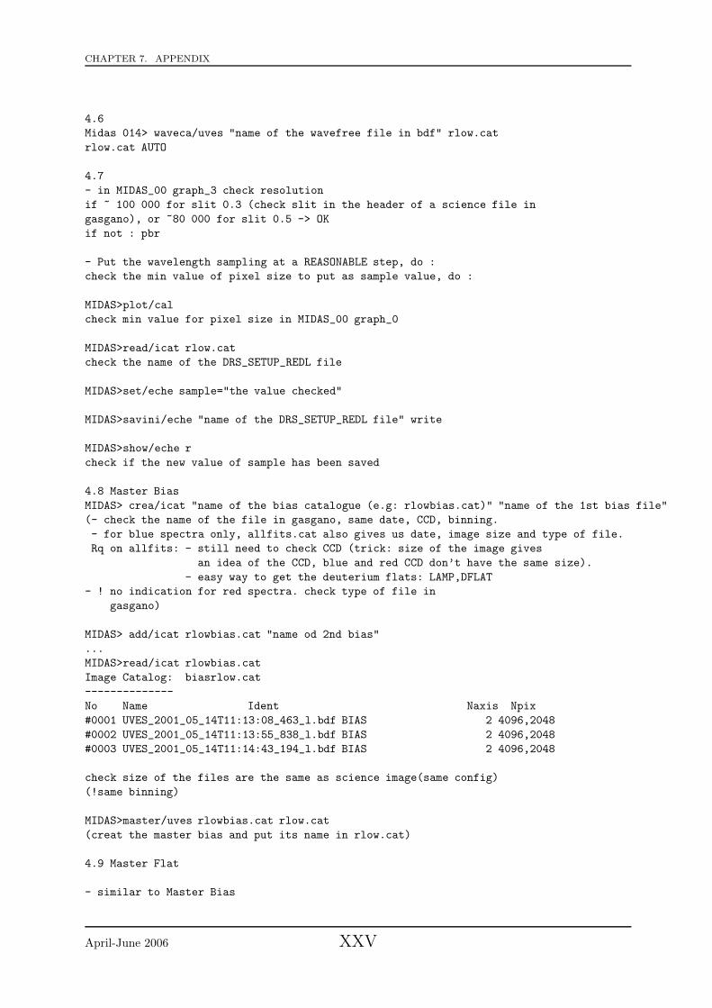
CHAPTER 7. APPENDIX

4.6

Midas 014> waveca/uves "name of the wavefree file in bdf" rlow.cat

rlow.cat AUTO

4.7

- in MIDAS_00 graph_3 check resolution

if ~ 100 000 for slit 0.3 (check slit in the header of a science file in

gasgano), or ~80 000 for slit 0.5 -> OK

if not : pbr

- Put the wavelength sampling at a REASONABLE step, do :

check the min value of pixel size to put as sample value, do :

MIDAS>plot/cal

check min value for pixel size in MIDAS_00 graph_0

MIDAS>read/icat rlow.cat

check the name of the DRS_SETUP_REDL file

MIDAS>set/eche sample="the value checked"

MIDAS>savini/eche "name of the DRS_SETUP_REDL file" write

MIDAS>show/eche r

check if the new value of sample has been saved

4.8 Master Bias

MIDAS> crea/icat "name of the bias catalogue (e.g: rlowbias.cat)" "name of the 1st bias file"

(- check the name of the file in gasgano, same date, CCD, binning.

- for blue spectra only, allfits.cat also gives us date, image size and type of file.

Rq on allfits: - still need to check CCD (trick: size of the image gives

an idea of the CCD, blue and red CCD don’t have the same size).

- easy way to get the deuterium flats: LAMP,DFLAT

- ! no indication for red spectra. check type of file in

gasgano)

MIDAS> add/icat rlowbias.cat "name od 2nd bias"

...

MIDAS>read/icat rlowbias.cat

Image Catalog: biasrlow.cat

--------------


#0001 UVES_2001_05_14T11:13:08_463_l.bdf BIAS 2 4096,2048

#0002 UVES_2001_05_14T11:13:55_838_l.bdf BIAS 2 4096,2048

#0003 UVES_2001_05_14T11:14:43_194_l.bdf BIAS 2 4096,2048

check size of the files are the same as science image(same config)

(!same binning)

MIDAS>master/uves rlowbias.cat rlow.cat

(creat the master bias and put its name in rlow.cat)

4.9 Master Flat

- similar to Master Bias

April-June 2006 XXV

CHAPTER 7. APPENDIX

crea/icat

(check the name of the file in gasgano, same date, CCD, central wlgth, binning

+ check lamp (=ThAr) for BLUE CCD bc Deuterium lamp has spectral lines in the

upper blue part of the spectrum)

add/icat

read/icat

MIDAS>master/uves rlowflat.cat rlow.cat rlow.cat

(creat the master flat and put its name in rlow.cat)

Midas> read/icat rlow.cat

Image Catalog: rlow.cat

--------------


#0001 o860L1x1.tbl ORDER_TABLE_REDL

#0002 b860L1x1.tbl BACKGR_TABLE_REDL

#0003 d860L1x1.tbl DRS_SETUP_REDL

#0004 l860REDL.tbl LINE_TABLE_REDL

#0005 thargood_2.tbl LINE_REFER_TABLE

#0006 l860L1x1_1.tbl LINE_TABLE_REDL1



#0009 mbREDL_1x1_l.bdf MASTER_BIAS_REDL 2 4096,2048

#0010 mf860_1x1_s04_l.bdf MASTER_FLAT_REDL 2 4096,2048

#0011 bg_860_1x1_s04_l.bdf BKG_FLAT_REDL 2 4096,2048

check - if all the files (11) are there

- if 860 (wavelength you are working on) everywhere

- if 1x1 everywhere (if a 2x2 appears : smth wrong)

--------------------------------------------------------------------------

4.10 to 4.14 to be done for each science spectra

------------------------------------------------

4.10 Change some values in the DRS_SETUP_REDL file

4.10.1 change slit value (parameter of Spectrum and Sky Extraction, do :

MIDAS> extract/image output = "name of science image.bdf"[@1500,<:@1500,>]

(1500 is the the # of the x column, < and > indicate all the lines in y)

MIDAS> assi/gra g,3

MIDAS> set/gra yaxis=100,400 xaxis=1000,1400 pmod=1

MIDAS> plot output

(In MIDAS_00 graph_3, see the orders of the science image, in the range chosen in set/gad

the slit is the width of an order)

MIDAS> get/gcursor

In MIDAS_00 graph_3, mesure the slit using the cursor. clic at each edge of an

order (avoid noisy bit). x values appear in MIDAS terminal. get delta(x).

exit window by right clic on the mouse

MIDAS>read/icat rlow.cat

check the name of the DRS_SETUP_REDL file

April-June 2006 XXVI

CHAPTER 7. APPENDIX

MIDAS>set/eche slit="value of delta(x)"


MIDAS>show/eche e

check if the new value of slit has been saved

.............................................

Tip : copy the following bit and paste it directly in MIDAS terminal

assi/gra g,3

set/gra yaxis=100,400 xaxis=1000,1400 pmod=1

plot output

get/gcursor

.............................................

4.10.2 change ron and conad in ccdfilt (parameter of Cosmic Rays Filtering), do :

- in gasgano, in the header of the science image, check value of ron and conad

MIDAS>set/eche ccdfilt="ron value","conad value","sigma(eg 4.0)"


MIDAS>show/eche c

check if the new value of ccdfilt has been saved

check if medfilt=1.0,1.0,100.0, if not do 4.10.3

4.10.3 change medfilt (parameter of Cosmic Rays Filtering), do :

MIDAS>set/eche medfilt=1.0,1.0,100.0


MIDAS>show/eche c

check if the new value of medfilt has been saved

4.11 START EXTRACTION

MIDAS> show/eche b

check if BKGMTD=POLY (Method of background fitting). if not, do:

MIDAS> set/eche BKGMTD=POLY

MIDAS> savini/eche "name of the DRS_SETUP_REDL file" write

MIDAS> show/eche b

check if the new value of BKGMTD has been saved

Midas 029> @@ reduce_filt "science bdf file (the same used in 4.10)"

"output catalogue (e.g : last.cat)" rlow.cat P AVERAGE

- Backgound fitting plotted in MIDAS_00 display_0, graph_1, graph_2, graph_3

- check in MIDAS_00 graph_1, graph_2, graph_3 if fit (colored line) is good

- if yes (most of the time), right clic on MIDAS_00 display_0.

reduce_filt will continues running. do 4.11.2

- if no, right clic on MIDAS_00 display_0 and ctrl-c in MIDAS terminal.

reduce_filt will stops running. do 4.11.1

4.11.1 Background correction (following of method of bkgrd fitting)

- change order of the polynomial fitting (parameter of Background)

April-June 2006 XXVII

CHAPTER 7. APPENDIX

MIDAS> set/eche BKGPOL=1,2

(4 is the order in x, 5 in y)

MIDAS> savini/eche "name of the DRS_SETUP_REDL file" write

MIDAS> show/eche b

check if the new value of BKGPOL has been saved



- check in MIDAS_00 graph_1, graph_2, graph_3 if fit (colored line) is good

- if yes (always), right clic on MIDAS_00 display_0.

reduce_filt will continues running. do 4.11.3

(if no, right clic on MIDAS_00 display_0 and ctrl+c in MIDAS terminal.

reduce_filt will stops running. .... now, umm ... ask Alex ;) )

4.11.3 Cosmic ray filtering

- Cosmic rays plotted in MIDAS_00 display_0

if cosmic well spread on the image : ok, right clic on display_0 and let

reduce_filt finish its run

if cosmic along trends (lines) : bad. right clic on display_0 and ctrl-c on MIDAS

terminal. higher last number of medfilts, do:

MIDAS>set/eche medfilt=1.0,1.0,120.0

-----


MIDAS>show/eche c

check if the new value of medfilt has been saved

4.11.4



when background on display_0 right clic to continue

when cosmic ray on display_0 right clic to continue

4.12

- creat a fits file from the reduced science image .bdf

Midas 159> outdisc/fits "name of output of reduce_filts (r_A_...bdf)" name=input?fits

creat a fits file, called "name".mt, in working directory (FITS/)

4.13

- in a terminal, in the FITS directory

>cp "name".mt ../Reduced/.

>mv ../Reduced/"name".mt ../Reduced/"name".fits

4.14

- check the reduced spectra "name".fits, using IRAF

April-June 2006 XXVIII

Documents

Calibration of effective temperature of solar type stars, using