Calibration and Validation of a Two- Dimensional Hydrodynamic

In cooperation with the Ohio River Valley Water Sanitation Commission

Calibration and Validation of a TwoDimensional Hydrodynamic Model of the Ohio River, Jefferson County, Kentucky

Water-Resources Investigations Report 01-4091

U.S. Department of the Interior U.S. Geological Survey

U.S. Department of the Interior U.S. Geological Survey

Calibration and Validation of a TwoDimensional Hydrodynamic Model of the Ohio River, Jefferson County, Kentucky

By Chad R. Wagner and David S. Mueller

Water-Resources Investigations Report 01-4091

In cooperation with the Ohio River Valley Water Sanitation Commission

Louisville, Kentucky

2001

U.S. DEPARTMENT OF THE INTERIOR GALE A. NORTON, Secretary

U.S. GEOLOGICAL SURVEY Charles G. Groat, Director

For additional information write to:

District Chief, Kentucky District U.S. Geological Survey 9818 Bluegrass Parkway Louisville, KY 40299-1906 http://ky. water.usgs.gov

Copies of this report can be purchased from:

U.S. Geological Survey Information Services Box 25286 Denver, CO 80225-0286

CONTENTS

Abstract............................................................................................................................................................ 1 Introduction...................................................................................................................................................... 1

Background............................................................................................................................................. 1 Purpose and scope .................................. .......................................... .......... ... . . ....................... .... .. .......... 2 Study area .................................................................................... ~.......................................................... 2

Model calibration and validation . . . . . .. . . . .. . .. . . . . . . . .. . . . . .. . . . . .. . . . . . . . . . . .. . . . . . . . .. . . . . . . . . . . . . . . . . . . . . . . . . . . . . . . . . . . . . . . .. . . . . . . . . ............ 4 Model description................................................................................................................................... 4 Field data collection and interpretation . . . .. . . . . . . . . . . . . . . . . . . . . . . .. . . ... . . . . . . . . . . . . . . . . . .. . . . . . . . . . . . . . . . . . . .. . . . . . . . . . . . . . . . . . .. . . . . . . 4

Water-surface elevations................................................................................................................ 8 Velocity and discharge................................................................................................................... 8 Bathymetry . .. ...... ... .... ... ... .......... .. .. ....... .............. ... ................ ... .. . .... .......................... ... .. .. .. ........... 8

Upstream river reach............................................................................................................................... 9 Computational-mesh configuration ... .. ... ..................... ................. ...................... .. . . ..... .. .. .. .. .. ........ · 9 Boundary conditions...................................................................................................................... 14 Calibration and validation results . . . . .. . . . . . . .. . . . . . . . . . . . . . . .. . . . .. . . . . . . . . . .. . . . .. . . . . . . . . .. . . . . . . . . . . . . . . . .. . . . . . . . . . . .. . . . . . . . . 14

Downstream river reach.......................................................................................................................... 15 Computational-mesh configuration ............................................................................................... 15 Boundary conditions...................................................................................................................... 21 Calibration and validation results . . . . .. . . . . . . . . . . . . . . . . .. . . . .. . . . . .. . .. . . . . . . . . . . . . . . . . . . . . . . . . . . .. . . . . . . . . . . .. . . . . . . . . . . . . . . . . .. . . 21

Summary and conclusions............................................................................................................................... 32 References cited............................................................................................................................................... 33

FIGURES

1-4. Maps showing: 1. Location of study area near Louisville, Kentucky . . . . . . . . . .. . . . . . . . . . . .. . . . . . . . . . . . . . . . . . . . . . . . . . . . . . . . . . . . . . . . . . . . . . 3 2. McAlpine Locks and Dam configuration and U.S. Geological Survey (USGS)

gaging station locations near Louisville, Kentucky . .. . . . . . . . . . . . . . . . . . . . . . . .. . . . . . . .. . . . . . . . . . . . . . . . . . . . . . . . . . . . . . . . 5 3. Location of hydrographic-survey cross sections, surveyed water-surface elevation

stations, and USGS gaging stations in the upstream study reach near Louisville, Kentucky................................................................................................................. 6

4. Location of hydrographic-survey cross sections, surveyed water-surface elevation stations, and USGS gaging stations in the downstream study reach near Louisville, Kentucky................................................................................................................. 7

5-21. Graphs showing: 5. Surface Water Modeling System (SMS) software triangulation of raw and straight-line

bathymetry data for a section of the upstream study reach in the Ohio River model simulation near Louisville, Kentucky . .. . . . . . . . . . . . . . . .. . . . . . . . . . . . . . . . . . . . . . . . . . . . . . . . . . . . . . . . . . . . . . . . . . . . . . . . . . . . . . . . . . . . . 10

6. Mesh configuration around the earthen dike adjacent to Louisville, Kentucky, and upstream of McAlpine Locks and Dam in the Ohio River model simulation .. ... . .. .. . . .. . .. ..... .. . . 11

7. Mesh configurations around Six- and Twelve-Mile Islands in the upstream Ohio River study reach . . . . . . . . . . . . . . . . . . . . . . . . . . . . . . . . . . . . . . . . . . . . . . . . . . . . . . . . . . . . . . . . . . . . . . . . . . . . . . . . . . . . . . . . . . . . . . . . . . . . . . . . . . . . . . . . . . . . . . .. . . . . . . . . 12

Contents Ill

8. Upstream reach mesh configuration around McAlpine Locks and Dam near Louisville, Kentucky . . . . . . . . . .. . .. . . . . . . . . . . . . . . . . . . . . . . . .. . . .. . . . . . . . . . .. . .. . . . . .. . .. . . . . . . . .. . . . . . . . . . . .. . . . . . . . . . . .. . . . . . . . . . . .. . 13

9. Field-measured and model-simulated velocity profiles for cross-section 5, . 13 miles upstream from McAlpine Locks and Dam ... ... . ... .. ............ ................... ......... ..... ....... 16

10. Field-measured and model-simulated low-flow, distance-weighted average cross-sectional velocities in the upstream study reach from the Ohio River model simulation . . . . . . . . . . . . . .. . . . . . . . . . . . . . . . . . . . . . . . . . . . . . . . . . .. . . . . . . . . . . . . . . . . . . . . . . . .. . . . .. . . . . . . . . . . .. . . . . . . . . . . .. . . . . . . . . . . . .. . . . . . . . . . . . . 17

11. Field-measured and model-simulated high-flow, distance-weighted average cross-sectional velocities in the upstream study reach from the Ohio River model simulation . . . . . . . . . . . . . .. . . . . . . . . . . . . . . . . . . . . . . . . . . . .. . .. . . . . .. . . . . . . . . . . . . . . . . . . . . . . . . . . . . . . . . . . . . . . . . . . . . . . . . . . . . . . . . . . . . . .. . . . . . . . . . . . . . 18

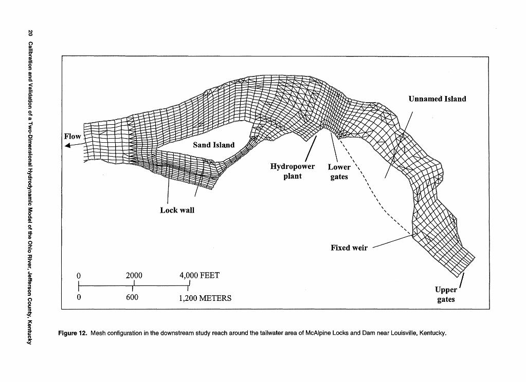
12. Mesh configuration in the downstream study reach around the tailwater area of McAlpine Locks and Dam ....................................................................................................... 20

13. Stage-discharge curve for McAlpine tailwater gaging station near Louisville, Kentucky, 1990-2000 .. ....... .. ... .. ........... ....... ..... ............. ... . .. . ....................................... ........ .. .. . 22

14. Stage-discharge curve at Kosmosdale gaging station near Louisville, Kentucky, 1995-2000................................................................................................................................. 23

15. Discharge-slope curve between McAlpine tailwater and Kosmosdale gaging stations near Louisville, Kentucky, 1995-2000 .. .. . . . . .. . . . . . . . . . . .. . . . . . . . . . . .. . . . . . . . . . . . . . . . . . .. . . . ... . . . . . . . . . .. . . . . . . . . . . .. . . 24

16. Field-measured and model-simulated low-flow velocity profiles for cross-sections 19 and 25 in the Ohio River model simulation.............................................................................. 26

17. Scatter plot of the cross-sectional area and average velocity differences between field measurements and model-simulated results for the 18 downstream Ohio River cross sections near Louisville, Kentucky . . . . . .. . . . . . . . . . . ... . . . . .. . . . . . . . . . . . . .. . .. . . .. . . . . . . . . . . . . . . .. . . . . . . .. .. . . . . . .. . 28

18. Comparison of cross-section 24 bathymetry in the downstream Ohio River study reach . ...... 29 19. Comparison of cross-section 20 bathymetry in the downstream Ohio River study reach . . . . . . . 29 20. Low-flow distance-weighted average cross-sectional velocity profile for the downstream

study reach in the Ohio River model simulation . . . . . . . . . . . . . . . . . . .. . .. . . . . . . . ... . . . . . . . . . .. . . . . . . . .. . .. . . . . . . . . . . . . . . 30 21. High-flow distance-weighted average cross-sectional velocity profile for the downstream

study reach in the Ohio River model simulation...................................................................... 31

TABLES

1. Summary of water-surface elevation calibration and validation for the upstream study reach in the Ohio River model simulation near Louisville, Kentucky . . . . . . . .. . . . . . . . . . . .. . .. . . . . . . . . . . . .. .. . . .. .. .. 14

2. Summary of flow-split calibration and validation for islands in the upstream study reach in the Ohio River model simulation .. . . . . . . . . . .. . . . . . . . . . . . . . . . . . . . . . . . . . . . . . .. . . . . . . . . . . . . . . . . .. . . . . . . . . . . . . . . . . . . . . . . .. . . . . . . . .. . .. . 19

3. Summary of continuity checks in the upstream Ohio River model simulation................................. 19 4. Evaluation of the Research Management Associates-2 (RMA-2) simulation representation

of the Ohio River rating developed for the downstream study reach near Louisville, Kentucky . . . . . . 25 5. Summary of water-surface elevation calibration and validation for the downstream study

reach in the Ohio River model simulation . .. .. . . . . . . . . . . .. . .. . . . . . . . . . . . . . . . . ... . . .. . . . . . .. . . . . . . . . . . . .. . . . . . . . . . . . . . . . . . .. . . . . .. . 25 6. Summary of continuity checks in the downstream Ohio River model simulation............................. 32

lv Contents

CONVERSION FACTORS AND VERTICAL DATUM

CONVERSION FACTORS

Multiply By To obtain

foot (ft) 0.3048 meter

foot per second (ftls) 0.3048 meter per second

cubic foot per second (ft3/s) 0.02832 cubic meter per second

mile (mi) 1.609 kilometer

VERTICAL DATUM

Sea level: In this report "sea level" refers to the National Geodetic Vertical Datum of 1929 (NGVD of 1929)-a geodetic datum derived from a general adjustment of the first-order level nets of both the United States and Canada, formerly called Sea Level Datum of 1929.

Elevation, as used in this report, refers to the distance above or below sea level.

Contents v

Calibration and Validation of a Two-Dimensional Hydrodynamic Model of the Ohio River, Jefferson County, Kentucky By Chad R. Wagner and David S. Mueller

Abstract

The quantification of current patterns is an essential component of a Water Quality Analysis Simulation Program (WASP) application in a riverine environment. The U.S. Geological Survey (USGS) provided a field validated two-dimensional Resource Management Associates-2 (RMA-2) hydrodynamic model capable of quantifying the steady-flow patterns in the Ohio River extending from river mile 590 to 630 for the Ohio River Valley Water Sanitation Commission (ORSANCO) water-quality modeling efforts on that reach. Because of the hydrodynamic

. complexities induced by McAlpine Locks and Dam (Ohio River mile 607), the model was split into two segments: an upstream reach, which extended from the dam upstream to the upper terminus of the study reach at Ohio River mile 590; and a downstream reach, which extended from the dam downstream to a lower terminus at Ohio River mile 636.

The model was calibrated to a low-flow hydraulic survey (approximately 35,000 cubic feet per second (ft3/s)) and verified with data collected during a high-flow survey (approximately 390,000 ft3/s). The model calibration and validation process included matching water-surface elevations at 10 locations and velocity profiles at 30 cross sections throughout the study reach. Based on the calibration and validation results, the model is a representative simulation of the Ohio River steady-flow patterns below discharges of approximately 400,000 f~/s.

INTRODUCTION

Combined sewer overflows (CSO's), sanitary sewer overflows (SSO's), nonpoint sources, and storm-water runoff are all sources of wet-weather pollution that contribute to the degradation of our Nation's vital water resources. In situations where more than one of these sources contributes to the impairment of water quality, a holistic approach defining the relative importance of each source's contribution to the problem is the most efficient way to arrive at an economical control plan. In order to determine the relative significance of the various sources of wet-weather pollution on major waterways, an understanding of the local hydrodynamics,pollutantlandloading,and pollutant-transport characteristics is essential.

Background

The Ohio River Valley Water Sanitation Commission (ORSANCO) is nearing completion of a national demonstration study to develop a waterquality model that is capable of simulating pollutant concentrations in the river during wet-weather periods and is able to quantify improvements to the water quality resulting from pollution control bestmanagement practices. The initial project was completed on a reach of the Ohio River, which included the Cincinnati/northern Kentucky metropolitan area. The Water Quality Analysis Simulation Program (WASP) was utilized to simulate the water-quality constituent transport and transformation during low-flow periods spanning the recreational-contact period May-September. The flow field required by WASP was simulated by use of a two-dimensional Resource Management Associates-2 (RMA-2) hydrodynamic model.

INTRODUCTION 1

In order to demonstrate the transferability of this project to other riverfront metropolitan areas, a similar study was initiated in the Louisville, Kentucky, metropolitan area; this study involved both hydrodynamic and water-quality modeling and field data collection. The U.S. Geological Survey (USGS), in cooperation with ORSANCO, developed a field-validated hydrodynamic model to support the water-quality model being developed by a consultant contracted by ORSANCO.

Purpose and Scope

This report describes the calibration and validation of the two-dimensional RMA-2 model to simulate the complex hydrodynamics of a 40-mi study reach of the Ohio River near Louisville, Ky. (Ohio River mile 590 to 630; fig. 1). The field data used to calibrate and validate the model also are described. Because of the hydrodynamic complexities induced by McAlpine Locks and Dam (Ohio River mile 607), the model was split into two segments: an upstream reach, which extended from the dam upstream to the upper terminus of the study reach at Ohio River mile 590; and a downstream reach, which extended from the dam downstream to a lower terminus at Ohio River mile 636.

Floodplains were not included in the model domain because of the project emphasis on low-flow periods spanning the recreational-contact period May-September. The final model was used to simulate the steady-flow patterns of the Ohio River for flows ranging from 6,500 to 197,700 ft3 Is. The lower-limit of the simulated flows (6,500 f~ls) is consistent with the discharge during a dye-tracing survey done by ORSANCO in September 1999. The upper limit of the range of simulated flows (197,700 ft31s) corresponds to the 90-percentile flow during the recreational-contact period based on historical discharge data during 1987-98. Although more historical discharge data are available, ORSANCO and the private consultant chose to use only recent data (1987-98) to determine the 90-percentile flow. The process and methodology

used to calibrate and validate the model with field data as well as the results of the model simulations are discussed in this report.

Study Area

The Ohio River study area begins at the northeast comer of Jefferson County, Ky., and extends southwestward through the county and ends 6 river miles downstream from the mouth of the Salt River (fig. 1). The upstream reach is in the McAlpine Locks and Dam pool and the water level is kept at an elevation of approximately 420 ft above sea level during low-flow periods. The .downstream reach of the study area is in the tailwater of McAlpine Locks and Dam. The water level at the dam is held at a normal pool level of 383 ft above sea level by the Cannelton Locks and Dam, which is located 150 river miles downstream. The channel has a generally trapezoidal geometry with steep banks rising at slopes greater than 22 percent (0.22 ft/ft). The banks along the upstream reach extend to an approximate elevation of 440 ft, whereas the banks of the downstream reach rise to approximately 420ft.

The following river characteristics were determined from the data collected during the hydrograJ?hiC surveys. At a discharge of 36,000 ~Is, the average depth of the river thalweg was approximately 30 ft in the upstream reach and 20 ft in the downstream reach. The average width of the river at a discharge of 36,000 ft3 Is was approximately 3,000 ft in the upstream reach and 1,600 ft in the downstream reach. A discharge of 390,000 f~ Is produced an average depth in the thalweg of approximately 45 ft in both the upstream and downstream reaches. The width of the river at a discharge of 390,000 ft31s was approximately 4,000 ft in the upstream reach and 2,500 ft in the downstream reach. The bank and bed material of the study reach varies between cohesive and noncohesive sediment. The bank vegetation predominately consists of small shrubbery and vegetation, void of large trees.

2 Calibration and Validation of a Two-Dimensional Hydrodynamic Model of the Ohio River, Jefferson County, Kentucky

86° 8& 45' 8&30 3~30~----------~--------------,.~--------------~~~

ron

Downstream model terminus

' -t

620

EXPLANATION

I )easure Rodge Parl<

j"lalley Sl etoon Bethany

• River mile marker 615 Ohio River Mile

Figure 1. Location of study area near Louisville, Kentucky.

Upstream model terminus

0 1 2 4 6 I

8 10 MILES

01 2 4 6 8 10 K ILOMETERS

INTRODUCTION 3

The structures that compose McAlpine Locks and Dam are located on the northwestern side of Louisville, Ky., and extend from Ohio River mile 604.4 to 607 .4. The current locks-and-dam configuration (fig. 2) consists of a hydroelectric powerhouse; two lock chambers (one 600 by 110 ft and the other 1,200 by 110 ft in length and width, respectively); nine tainter gates, four near the powerhouse and five just upstream of the Conrail Railroad Bridge; and a fixed weir with a crest at an elevation of 422ft at the downstream gates, incrementally raised to an elevation of 423 ft at the upper set of gates. An earthen dike was constructed at the upstream end of Shippingport Island to reduce the crosscurrents affecting vessels navigating the lock canal. The shoal area that exists downstream from the upper gates and fixed weir is referred to as the Falls of the Ohio and is an area of archeological importance. To facilitate public use of the fossil beds at the Falls of the Ohio, the U.S. Army Corps of Engineers (COE) has agreed to a 2-month operational period (typically August-October) each year when the fixed weir and upper gates are not used to pass flow, except for extreme hydrological events. Under low flow or when the upper gates of McAlpine Locks and Dam are not in operation, the Falls of the Ohio is an area of slack flow.

MODEL CALIBRATION AND VALIDATION

At least two data sets are required to adequately calibrate and validate a numerical model. The general procedure used to calibrate and . validate the RMA-2 model was to first collect field data in order to develop the computational mesh. The model then was calibrated to the water-surface elevations and velocities observed in the field for the initial flow. A second flow condition then was simulated without changing the computational mesh or model parameters, and the simulated watersurface elevations and velocities were compared with those observed in the field for this second flow condition.

Model Description

RMA-2 is a two-dimensional depth-averaged finite-element hydrodynamic numerical model capable of computing water-surface elevations and

horizontal-velocity components for subcritical, freesurface flow in two-dimensional flow fields (U.S. Army Corps of Engineers, 1997). The model is designed for problems in which vertical accelerations are negligible, and velocity vectors generally point in the same direction over the entire depth of the water column at any discrete period in

time. Typical applications of the RMA-2 numerical

model include calculating water-surface elevations and flow distribution around islands; flow patterns at bridges having one or more relief openings, in contracting and expanding reaches, into and out of off-channel hydropower plants, and at river junctions; circulation and transport in water bodies with wetlands; and water levels and flow patterns in rivers, reservoirs, and estuaries.

One of the predominating operating assumptions in RMA-2 is that acceleration of flow in the vertical direction is negligible. The model is not intended for applications in which vortexes, vibrations, or vertical accelerations are the primary interests; therefore, the simulation of vertically stratified flow fields is beyond the capabilities of RMA-2 (U.S. Army Corps of Engineers, 1997).

Field Data Collection and Interpretation

Water-surface elevations, channelbathymetry, and detailed water-velocity measurements were collected at two different flow conditions (36,000 and 390,000 ft3 /s) and used in the model for calibration and validation, respectively. Water-sUrface elevations were measured at 10 locations ( 4 upstream and 6 downstream) along the study reach concurrent with both hydraulic surveys. Detailed water-velocity measurements and channel-bathymetry data were collected at 30 cross sections ( 12 upstream and 18 downstream)--spaced approximately 1.5 mi apart--during each of the hydraulic surveys (figs. 3 and 4). A separate data-collection trip from the two hydrographic surveys was used to collect channelbathymetry data in sufficient detail for the development of a computational mesh.


3: 0 c m r 0 )> r a; JJ

~ 0 z )> z c < )> r c )> ~

0 z

0 .25 .50

~Upper gates

.. ""- Earthen dike

.75 1 MILE

0 .25 .50 .75 1 KILOMETER EXPLANATION

(%) USGS gaging station location

03294600 USGS gaging station number

• • Continuity check line

CC3 Continuity line name

Figure 2. McAlpine Locks and Dam configuration and U.S. Geological Survey (USGS) gaging station locations near Louisville, Kentucky.

3ff25 -

8E?45 I

85l35 I

/ -Goshen

\ '- \

~,,)

' -..... /

,.-> (ill)

:r

Twelve-Mile Island

Six- Mile Island

0 2

'

--

3 4 MILES

0 2 3 4 KILOMETERS

EXPLANATION

<1) USGS gaging station location - Survey cross section

03294600 USGS gaging station number * Surveyed water-surface elevation location

1 0 Cross-section number

e River mile marker

600 Ohio River Mile

Figure 3. Location of hydrographic-survey cross sections, surveyed water-surface elevation stations, and U.S. Geological Survey (USGS) gaging stations in the upstream study reach near Louisville, Kentucky.


8&01' I

3s016' -

8&53 ...___- - ...... ~ ..... _____ ,// I

---~~-_, ( r

L - .-'\ I I . ..-

.. -_'r··· )

8&45 ... I

_________ ./' l L

3ff -

<I> 03294600

*

(

L -+-.1 '•

(

./L__

\ . ..--~ ,-·

I

_ ...

. .. ... -

_}

·"'" -----·"'"

~aft Aiv .. . f 'ldl' . - - er .r•n-.: 1 lil 1te

--....... __ ,.,... ___ _

t~. aaemen '' e 0 2 3 4 5 MILES

0 2 3 4 5 KILOMETERS EXPLANATION

USGS gaging station location

USGS gaging station number

Surveyed water-surface elevation location

.._. Survey cross section

1 0 Cross-section number

e River mile marker

600 Ohio River Mile

Figure 4. Location of hydrographic-survey cross sections, surveyed water-surface elevation stations, and U.S. Geological Survey (USGS) gaging stations in the downstream study reach near Louisville , Kentucky.

MODEL CALIBRATION AND VALIDATION 7

Water-Surface Elevations

Water-surface elevations at the seven locations throughout the reach (figs. 3 and 4) were surveyed with a total station. To document the changes in river stage during a hydraulic survey, the water-surface elevations were sl:rrveyed in the morning and then again in the afternoon. The average water-surface elevation was used to determine a water-surface slope corresponding to the average discharge measured during the survey.

The 40-mi study section of the Ohio River includes a total of four USGS stream gages-two each in both the upstream and downstream reaches. Both upstream gages--one located on the Second Street Bridge (number 03293548) and the other at Indiana Pass (number 03293550)-are located near river mile 604 and provided to assist the COE, Louisville District in maintaining the McAlpine Locks and Dam normal pool elevation. The Second Street Bridge gage is located on a pier near the center of the channel about 4,000 ft upstream from McAlpine Locks and Dam; the Indiana Pass gage is located on the Indiana shore about 500 ft downstream from the Second Street Bridge gage (fig. 3). The McAlpine tailwater and Kosmosdale gaging stations (numbers 03294500 and 03294600, respectively) are located within the downstream reach (fig. 4). The McAlpine tailwater gage is located near the Kentucky shore on the downstream end of the lock guide wall (river mile 607). The Kosmosdale gage is located on the Kentucky shore,. 19.8 mi downstream from the tailwater gage (river mile 628).

Velocity and Discharge

Water-velocity and discharge data were collected from a moving boat. The horizontal position of the boat was measured using a . differentially corrected global positioning system (DGPS) receiver. The DGPS system used receives its differential corrections from a commercial service's communications satellite. The unit is specified by the manufacturer to be accurate to 3.3 ft

at two standard deviations; tests and prior use of this unit indicate that typically about 80 percent of the data are within 3.3 ft of the true location.

Recent advances in velocity-measurement technology allow three-dimensional velocities to be collected from a moving boat using an ~coustic Doppler current profiler (ADCP) (Oberg and Mueller, 1994; Mueller, 1996). All velocities were measured with an ADCP. The ADCP allows threedimensional velocities to be measured from approximately 4 ft beneath the water surface to within 6 percent of the depth to the bottom. Established methods were used to estimate the discharge in the unmeasured top and bottom portions of the profile (Simpson and Oltmann, 1991). Cross-sectional average velocities were computed by dividing the measured discharge by the measured cross-sectional area. In addition, depth-averaged velocities were computed for subsections of the flow in each cross section; however, these discrete depth-averaged velocities were computed as an average of the measured velocity and did not account for the velocity in the unmeasured portions of the water column.

In order to compensate for the slight changes in discharge of the river during the survey, all the discharge measurements collected were averaged to produce a flow rate that was representative of the entire survey period. The time necessary to complete a hydraulic survey on each of the simulated sections did not permit both the upstream and downstream reaches to be surveyed on the same day; therefore, minor differences are present in the discharge measurements used to calibrate and validate the upper and lower models.

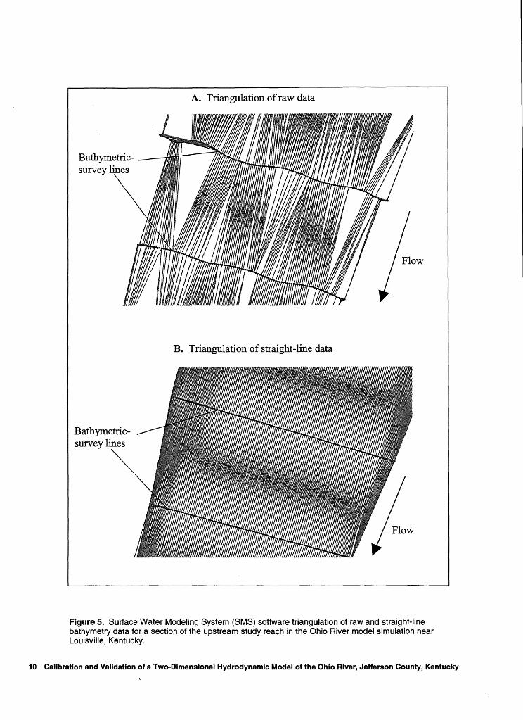
Bathymetry

Bathymetry data also were collected from a moving boat. The horizontal position of the boat was measured using the DGPS receiver. During the initial low-water survey, a 200-kHz echo sounder was used to measure the channel bathymetry at the 30 predefined cross sections.

8 Calibration and Validation ~fa Two-Dimensional Hydrodynamic Model of the Ohio River, Jefferson County, Kentucky

The channel bathymetry obtained from the initial bathymetric survey at the 30 velocitymeasurement cross sections was compared to the 1963 COE hydrographic survey of the area. The surveyed data points of the 1963 hydrographic survey were digitized along straight cross sections spaced at 114-mi intervals and oriented perpendicular to flow. All data points were digitized from paper maps. A triangulated irregular network (TIN) of the 1963 data was generated to extract cross sections from the 1963 data for the 30 locations surveyed for this project. The shapes of the cross sections measured in the downstream reach were similar to cross sections extracted from the 1963 hydrographic-survey data. Differences in elevation were within the errors expected from the survey technologies of 1963 and those used in this survey; therefore, data from the 1963 hydrographic survey were used for the channel bathymetry in the downstream hydrodynamic model. The shape of the cross sections measured in the upstream reach displayed differences from the cross sections extracted from the 1963 hydrographic-survey data; therefore, a second bathymetric survey of the upstream reach was completed with cross sections spaced approximately 1,000 ft apart. The data from the second bathymetry survey was used for the channel bathymetry in the upstream hydrodynamic model.

Bathymetric data surveyed with the echo sounder in the upstream reach did not fall on perfectly straight cross sections because of inconsistencies in the boat course across the river. The internal triangulation routine done by the RMA-2 interface software package--Surface-water Modeling Systems (SMS), version 7.0 (Brigham Young University, 1999)-did not properly interpret the collected bathymetry data, resulting in triangulation within the same cross section and a large portion of the area between two cross sections estimated with only three data points. An example of the raw-data triangulation is presented in figure 5a. The raw data collected along each cross section was mathematically forced onto a straight line andre-triangulated; figure 5b shows the re-triangulation of the section shown in figure 5a.

Although forcing the data points onto a straight line

does introduce some error, the straight -line cross

sections produced a better representation of the

upstream channel bathymetry than the unadjusted data.

Upstream River Reach

The simulated upstream reach begins 3 mi

upstream of the Jefferson/Oldham County line

(Ohio River mile 590) in Kentucky, and extends downstream to McAlpine Locks and Dam (Ohio

River mile 607). Two islands are present that add

hydraulic complexities to this reach: Twelve-Mile

Island located at Ohio River mile 593, and Six-Mile

Island located at Ohio River mile 598. The

configuration of McAlpine Locks and Dam includes

upper and lower sets of tainter gates and a

hydropower plant that served as downstream

boundary conditions for the model.

Computational-Mesh Configuration

The finite-element network for the upstream

river reach consisted of 6,920 elements. The islands

and dike were simulated by installing gaps in the

mesh because the simulated flows did not overtop

these features (figs. 6 and 7). The boundary nodes at

the upstream and downstream points of the islands

were specified as "stagnation points" (locations of

zero velocity). These specifications generally are

located in comers of grids or along boundaries with relatively negligible flow velocities and are applied

to reduce artificial loss of discharge out of the

channel boundaries. The resolution of the grid was

increased in the area around McAlpine Locks and

Dam in order to reproduce the hydraulic

complexities induced by these structures (fig. 8). In order to maintain numerical stability, the sloping

banks were truncated at an elevation of 418 ft.

Above this elevation, the banks were assumed to be

vertical walls.


A. Triangulation of raw data

B. Triangulation of straight-line data

Figure 5. Surface Water Modeling System (SMS) software triangulation of raw and straight-line bathymetry data for a section of the upstream study reach in the Ohio River model simulation near Louisville, Kentucky.


3: 0 0 m r (') )> r a; JJ )> -i 0 z )> z 0 < )> r 6 )> -i 5 z ..... .....

Shippingport Island

Earthen dike

0

I 0

500 I I

150

1,000 FEET I I

300 METERS

Figure 6. Mesh configuration around the earthen dike adjacent to Louisville, Kentucky, and upstream of McAlpine Locks and Dam in the Ohio River model simulation near Louisville, Kentucky.

A. Mesh configuration around Six-Mile Island

Six -Mile Island

B. Mesh configuration around Twelve-Mile Island

Twelve-Mile Island

0 .25 .50 .75 I I I I I I I I

1 MILE I

0 .25 .50 .75 1 KILOMETER

Figure 7. Mesh configurations around Six- and Twelve-Mile Islands in the upstream Ohio River study reach near Louisville, Kentucky.


3:: 0 c m r-

~ r-a; ::tJ

~ 0 z )> z c < )> r-6 ~ 0 z

Hydropower plant

Shippingport Island

Earthen dike

0

I 0

Upper gates

I .25

.25 I

I .50

Figure 8. Upstream reach mesh configuration around McAlpine Locks and Dam near Louisville, Kentucky.

.50

I .75

I .75 1 MlLE

I 1 KILOMETER

Boundary Conditions

Steady-state discharges of 34,000 and 383,000 f0 Is were used to calibrate and validate the model. These discharges were used as the upstreamboundary condition for the model and the lateralflow distribution was assumed to be uniform across the inflow boundary for both discharges.

The downstream-boundary condition consisted of outflows through the lower gates and hydropower plant (low-flow only) and a head condition assigned to the upper g,ates. The lower set of tainter gates carried 14,000 ft' Is, whereas the hydropower plant passed the remalning 20,000 f~ Is under the low-flow condition. At 383,000 f2 Is, the flow is divided between the upper and lower gates, with 126,350 ft31s passing through the lower gates and the remaining 256,650 tt3 Is passing through the upper gates. The McAlpine Locks and Dam pool elevations for both discharges were determined from the USGS gaging station records at Indian Pass (number 03293550) and Second Street Bridge (number 03293548). Normal pool elevation (419.6 ft) was used for 34,000 ft31s flow, and a pool elevation of 423.9 ft was used for 383,000 ft31s flow.

Calibration and Validation Results

Data from the low-flow (34,000 ft31s) hydraulic survey were used to calibrate the model, and data from the high-flow (383,000 ft31s) survey

were used to validate the model. The calibration and

validation process consisted of comparing the

simulated water-surface elevations at the

4 upstream water-surface-elevation stations and

12 cross-sectional velocity profiles with those

surveyed in the field. A Manning's roughness

coefficient (n) was assigned to each element and

iteratively adjusted until the model adequately

simulated the surveyed water-surface elevations and

velocity profiles.

Inspection of the velocity profiles collected in

the field revealed no-slip conditions along the

riverbanks, indicating that the shear stress along the

banks is great enough to cause the tangential

velocity to approach zero. To simulate this

characteristic with RMA-2, the Manning's n value

was increased to 0.035 for one row of elements

along the outer boundary of the mesh. The

calibrated Manning's n in the remainder of the

channel was 0.024. This combination produced the

best simulation of water-surface elevation (table 1),

velocity magnitudes, and lateral-velocity

distribution for both low- and high-flow conditions.

Matching the high-flow water-surface elevations

verified that the area lost by truncating the banks

was negligible in the model simulation.

Table 1. Summary of water-surface elevation calibration and validation for the upstream study reach in the Ohio River model simulation near Louisville, Kentucky

(8/13/98) Low-flow condition (2/16/00) High-flow condition

Field Model Field Model water-surface water-surface water-surface water-surface

elevation elevation elevation elevation (feet above (feet above (feet above (feet above

Station sea level) sea level) Difference 1 sea level) sea level) Difference 1

Harmony Landing 419.99 419.66 -0.33 427.59 427.68 0.09

Louisville Water Company 419.91 419.64 -.27 426.51 426.46 -.05

Cox's Park Well 419.86 419.62 -.24 425.19 425.04 -.15

Indiana Pass 419.60 419.60 0 423.88 423.90 .02

1 Differences are determined by subtracting field from model-simulated water-surface elevation.


The simulated velocity magnitudes and

distributions compared well with the field

measurements. A comparison of the model and

field-velocity profiles for cross-section number 5

(13 mi upstream from McAlpine Locks and Dam)

is shown in figure 9. The shape of the field- and

model-velocity distributions were similar, whereas

on average, the velocity magnitudes were within

0.1 ft/s. The average cross-sectional velocities for

the 12 cross sections also were compared. The

model adequately reproduced the average field

velocities (figs. 10 and 11). The model also

accurately reproduced the measured-flow

distributions around Twelve- and Six-Mile Islands

(table 2).

Continuity was checked throughout the

downstream model to assure that mass was being

conserved. The model conserved mass throughout

the reach under high flow, but a 3 percent loss

resulted under low flow in the approach to the lower

tainter gates and hydropower plant (table 3). A

tolerance of +1- 3 percent in mass-conservation

discrepancy is typically acceptable for most models

(U.S. Army Corps of Engineers, 1997). Algorithms

used to import RMA-2 output into the WASP water

quality model can correct for mass-conservation

discrepancies.

Downstream River Reach

The simulated reach· begins at the McAlpine

Locks and Dam (Ohio River mile 607) and extends

downstream to Ohio River mile 636, 6 mi downstream from the mouth of the Salt River. This

section of the model includes part of the Cannelton

Locks and Dam pool, which is held at a normal pool

elevation of 383 ft. The two sets of tainter gates, the

hydropower plant, a lock wall supported on piles

that allows flow beneath the wall, and Sand Island

. all contribute to the hydraulic complexities of the

area located immediately downstream of the

McAlpine Locks and Dam.

Computational-Mesh Configuration

The finite-element network for the

downstream river reach consisted of

10,803 elements. In order to maintain numerical

stability, the sloping banks were truncated at an

elevation of 380 ft. Above this elevation, the banks

were assumed to be vertical walls.

Sand Island and an unnamed island in the

Falls of the Ohio region were simulated by

installing gaps in the mesh at the location of these

features. The resolution of the grid is increased in

the area around Sand Island, the hydropower plant,

the lock wall, and both sets of tainter gates to

improve simulation of the hydraulic complexities

induced by these structures (fig. 12). In order to

simulate the passage of flow under the lock wall, an

increased Manning's roughness value (n =.50) was

assigned to the elements representing the lock wall;

this value allowed flow through the elements under .

a much greater resistance. Stagnation points were

created at sharp break points along Sand Island and

the mesh boundary in the area of the lower tainter

gates to reduce artificial loss of discharge through

the boundaries.


0 z 0 0.6 (.) w Cl)

a:: w D..

tu 0.4 w LL

~

~ (.) 0 0.2 ..J w >

A. Low-flow velocity profile comparison

--Field ......_Model

0.0~--~----~----~----~----~----~----~----~--~

0 200 400 600 800 1,000 1,200 1,400 1,600 1,800

DISTANCE FROM LEFT BANK, IN FEET

B. High-flow velocity profile comparison

6r---~.---~.---~----~----~----~-----r----~----~

0 z 0 (.) w

5

UJ 4 c::: w D..

~ 3 LL

~

~- 2 (.)

0 ..J

~

_.Field ......_Model

0~--~----~----~----~----~----~----~----~----~

0 200 400 600 800 1,000 1,200 1,400 1,600 1,800


Figure 9. Field-measured and model-simulated velocity profiles for cross-section 5, 13 miles upstream from McAlpine Locks and Dam near Louisville, Kentucky.

16 Calibration and Validation of a Two-Dimensional Hydrodynamic Model ofthe Ohio River, Jefferson County, Kentucky

3:: 0 c m r-

~ r-a;

~ 0 z )> z c

~ r-6 ~ 0 z ..... -..1

O 7 r c:::::::J Field · -Model .67

~~ 0.6 ()

0 _J

w > 0.5 _J

~ 0 0 z - 0 0.4 ~ () () w ~ (/)

I 0:: (j) w 0.3 (j) a_ 0 ~ 0::: w () w w u.. 0.2 (!) z ~ w ~ 0.1

0 1 2 3R 3L 4 5 6 ?R ?L 8 9 10 11 12

CROSS SECTION, IN DOWNSTREAM ORDER

Figure 10. Field-measured and model-simulated low-flow, distance-weighted average cross-sectional velocities in the upstream study reach from the Ohio River model simulation near Louisville, Kentucky.

..6 o:>

~ s= iii :::t 0 ::::s C» ::::s Q.

< !. s: C» :::t o::::s

a C»

~ <? 0

~ ::::s 0 0 ::::s !. :::r:: '< Q.

j ::::s C» 3 c;

== &. !. a ~ Cl)

0 ::::J" 0 :::0

~ .:"' c.. Cl)

;: (3 0 ::::s

~ c ::::s

~ ~ ~ n ~

~~ 5 5 I r=- 1 Field

· Model

() 5.0 0 _J

4.5 w > _J <( 0 4.0 z z 0 8 3.5 b w w (/) 3.0 (/) 0:.:: ch w (/) 0.. 2.5 0 J-0:.:: w () w 2.0

LL w z (!) - 1.5

~ 1.0 w

~ 0.5

0 1 2 3R 3L 4 5 6 7R 7L 8 9 10 11 12

CROSS SECTION, IN DOWNSTREAM ORDER

Figure 11. Field-measured and model-simulated high-flow, distance-weighted average cross-sectional velocities in the upstream study reach from the Ohio River model simulation near Louisville, Kentucky.

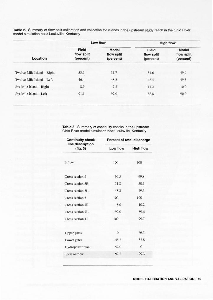
Table 2. Summary of flow-split calibration and validation for islands in the upstream study reach in the Ohio River model simulation near Louisville, Kentucky

Low flow High flow

Field Model Field Model flow split flow split flow split flow split

Location (percent) (percent) (percent) (percent)

Twelve-Mile I land - Right 53.6 51.7 51.6 49.9

Twelve-Mile Island- Left 46.4 48.3 48.4 49.5

Six-Mile Island - Right 8.9 7.8 1 1.2 10.0

Six-Mile Island - Left 91.1 92.0 88.8 90.0

Table 3. Summary of continuity checks in the upstream Ohio River model simulation near Louisville, Kentucky

Continuity check Percent of total discharge line description

(fig. 3) Low flow High flow

Inflow 100 100

Cross ection 2 99.5 99.8

Cross section 3R 51.8 50.1

Cross section 3L 48.2 49.5

Cross section 5 100 100

Cross section 7R 8.0 10.2

Cross section 7L 92.0 89.6

Cross section I I 100 99.7

Upper gate 0 66.5

Lower gates 45 .2 32.8

Hydropower plant 52.0 0

Total outflow 97 .2 99.3


N 0

0 !!. c: ~ 0 :::s A) :::s c. < !!. a: ! 0 :::s a A)

~ 9 c ~ :::s en 0 :::s !!. ::1: '< c.

j :::s A)

3 cr == 8. !. a :;t (I)

0 :::J' 0 :::D

~ :" c:..

i UJ 0 :::s g c :::s ~ ~ :::s

0

I 0

2000 I I

600

Lock wall

4,000 FEET I I

1 ,200 METERS

Lower gates

\ \

\ \

\ \

\

Fixed weir

\ \

\ \

\ \

\ \

\ \

' '

Unnamed Island

'

2' Figure 12. Mesh configuration in the downstream study reach around the tailwater area of McAlpine Locks and Dam near Louisville, Kentucky. ()

~

Boundary Conditions

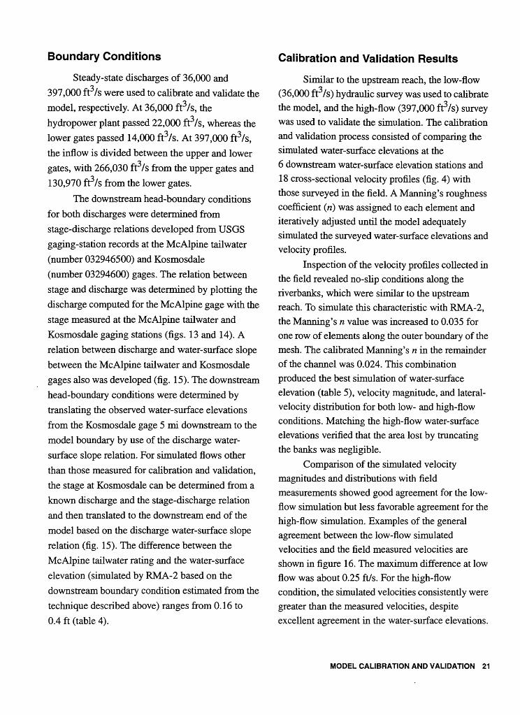
Steady-state discharges of 36,000 and

397,000 ft3 Is were used to calibrate and validate the

model, respectively. At 36,000 ft3 Is, the

hydropower plant passed 22,000 ft3 Is, whereas the

lower gates passed 14,000 tt31s. At 397,000 ft3/s,

the inflow is divided between the upper and lower

gates, with 266,030 ft3 Is from the upper gates and

130,970 f21s from the lower gates.

The downstream head-boundary conditions

for both discharges were determined from

stage-discharge relations developed from USGS

gaging-station records at the McAlpine tail water

(number 032946500) and Kosmosdale

(number 03294600) gages. The relation between

stage and discharge was determined by plotting the

discharge computed for the McAlpine gage with the

stage measured at the McAlpine tail water and

Kosmosdale gaging stations (figs. 13 and 14). A

relation between discharge and water-surface slope

between the McAlpine tail water and Kosmosdale

gages also was developed (fig. 15). The downstream

head-boundary conditions were determined by

translating the observed water-surface elevations

from the Kosmosdale gage 5 mi downstream to the

model boundary by use of the discharge water

surface slope relation. For simulated flows other

than those measured for calibration and validation,

the stage at Kosmosdale can be determined from a

known discharge and the stage-discharge relation

and then translated to the downstream end of the

model based on the discharge water-surface slope

relation (fig. 15). The difference between the

McAlpine tail water rating and the water-surface

elevation (simulated by RMA-2 based on the

downstream boundary condition estimated from the

technique described above) ranges from 0.16 to

0.4 ft (table 4).

Calibration and Validation Results

Similar to the upstream reach, the low-flow

(36,000 ft3 Is) hydraulic survey was used to calibrate

the model, and the high-flow (397,000 tt31s) survey

was used to validate the simulation. The calibration

and validation process consisted of comparing the

simulated water-surface elevations at the

6 downstream water-surface elevation stations and

18 cross-sectional velocity profiles (fig. 4) with

those surveyed in the field. A Manning's roughness

coefficient (n) was assigned to each element and

iteratively adjusted until the model adequately

simulated the surveyed water-surface elevations and

velocity profiles.

Inspection of the velocity profiles collected in

the field revealed no-slip conditions along the

riverbanks, which were similar to the upstream

reach. To simulate this characteristic with RMA-2,

the Manning's n value was increased to 0.035 for

one row of elements along the outer boundary of the

mesh. The calibrated Manning's n in the remainder

of the channel was 0.024. This combination

produced the best simulation of water-surface

elevation (table 5), velocity magnitude, and lateral

velocity distribution for both low- and high-flow

conditions. Matching the high-flow water-surface

elevations verified that the area lost by truncating

the banks was negligible.

Comparison of the simulated velocity

magnitudes and distributions with field

measurements showed good agreement for the low

flow simulation but less favorable agreement for the

high-flow simulation. Examples of the general

agreement between the low-flow simulated

velocities and the field measured velocities are

shown in figure 16. The maximum difference at low

flow was about 0.25 ft/s. For the high-flow

condition, the simulated velocities consistently were

greater than the measured velocities, despite

excellent agreement in the water-surface elevations.


_J

w > w _J

0:: <( w w ~ ~ ~ 6 ~ ~ w ..... z ttl a.. u.. _J z <(

(.) z ~ 0 ~ ..... z ~ o en

W~ ~ (!)

u1 ~

403 ~~~--~~--~~~--~~--~~--~~~--~~--~~~~

402 401 400 399 398 397 396 395 394 393 392 391 390 389 388 387 386 385 384 383

0

+

+ + + +

+ + +

+

+

+

50,000 100,000 150,000

DISCHARGE, IN CUBIC FEET PER SECOND

+

+

Best-fit line

200,000

Figure 13. Stage-discharge curve for McAlpine tailwater gaging station near Louisville, Kentucky, 1990-2000.

:!!: 0 c m r (') )> r a;

~ 0 z )> z c < )> r 8 ~ 5 z

z 0 I-

~ (/)

(!) z (!)

(3 w .....1 .....1 w c:x: > 0 w (/) c:x: 0 .....1 ~ c:x: (/) w 0 (/) ~ w ~ 6 z m 0 c:x:

~ ~ w u.. .....1 z w

4oo~~~~~~--~~--~~--~~--~~--~~--~~--~+--~~~

399

398

397

396

395

394

393 392

391

390

389

388 387

386

385

384

383

Best-fit line

+

+

+ +

+

+

+

+

382~~~~~~--~~--~~--~~--~~--~~--~~~--~~~

0 50,000 100,000 150,000 200,000

DISCHARGE, IN CUBIC FEET PER SECOND

Figure 14. Stage-discharge curve at Kosmosdale gaging station near Louisville, Kentucky, 1995-2000.

flo) ~

(') !. w c;: ....J 6.0e-5 ; <( + ... 0 0 :::J (/) + II)

0 + + + + :::J c. ~ < + + +

!. (/) 5.0e-5 + ++ a: 0

II) ~ + +++ ct

0 0 :::J + * 0 z -II) <(

~ 0::: 4.0e-5 + 9 w ..... + c

~ + + + ~ 0 \ + +

~ 0 + *+ :::J LL * + (I)

0 ....J 0::: :::J

~ !. w + + + + :::t a. 3.0e-5 '< w

b +-t + + + c. ... z +if-+ ++ ! a. 0 + :::J ....J LL II) + 3 <( z n () 2.0e-5 == ~ 0 (/)

+ c. z z !.. s. w 0 w ..... + ... ::r

~ (I)

~ 0 1.0e-5 + + ::r w (/) ++ 0 OJ :xJ (!) + ~ w z a. .:" 0 (!) + c.. + (I) ....J <( ;: (/) (!) ~ 50,000 100,000 150,000 200,000 0 :::J

&> DISCHARGE, IN CUBIC FEET PER SECOND c

:::J

~ ~ :::J ... Figure 15. Discharge-slope curve between McAlpine tailwater and Kosmosdale gaging stations near Louisville, Kentucky, c (')

1995-2000. ~

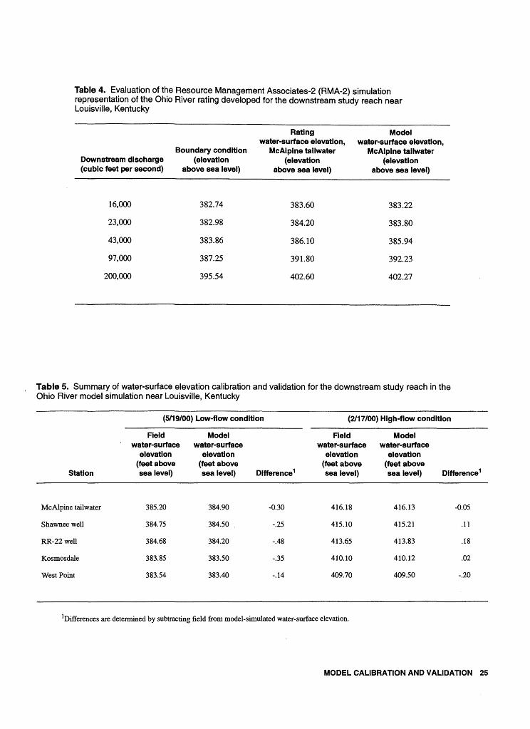
Table 4. Evaluation of the Resource Management Associates-2 (RMA-2) simulation representation of the Ohio River rating developed for the downstream study reach near Louisville, Kentucky

Rating Model water-surface elevation, water-surface elevation,

Boundary condition McAlpine tallwater McAlpine tallwater Downstream discharge (elevation (elevation (elevation (cubic feet per second) above sea level} above sea level) above sea level}

16,000 382.74 383.60 383.22

23,000 382.98 384.20 383.80

43,000 383.86 386.10 385.94

97,000 387.25 391.80 392.23

200,000 395.54 402.60 402.27

Table 5. Summary of water-surface elevation calibration and validation for the downstream study reach in the Ohio River model simulation near Louisville, Kentucky

(5119/00} Low-flow condition (2/17/00) High-flow condition

Field Model Aeld Model water-surface water-surface water-surface water-surface

elevation elevation elevation elevation (feet above (feet above (feet above (feet above

Station sea level) sea level) Difference 1 sea level) sea level) Difference 1

McAlpine tailwater 385.20 384.90 -0.30 416.18 416.13 -0.05

Shawnee well 384.75 384.50 -.25 415.10 415.21 .11

RR-22 well 384.68 384.20 -.48 413.65 413.83 .18

Kosmosdale 383.85 383.50 -.35 410.10 410.12 .02

WestPoint 383.54 383.40 -.14 409.70 409.50 -.20

1Differences are determined by subtracting field from model-simulated water-surface elevation.


c z

1.75

0 1.50 0 w en ffi 1.25 D.

t:i w 1.00 u. ~ ~ 0.75

0 g 0.50

~ 0.25

A. Low-flow velocity profile for cross-section 19

-Field _._ Model

o.ooL-----~-----L----~----~~----~----~----~----~ 0

1.75

1.50 c z 0 0 1.25 w en

" w D. 1.00 t:i w u. ~ 0.75

~ 0

0.50 g w >

0.25

0.00 0

200 400 600 800 1,000 1,200 1,400


B. Low-flow velocity profile for cross-section 25

200 400 600 800 1,000

-Field ......,_. Model

1,200 1,400


1,600

1,600

Figure 16. Field-measured and model-simulated low-flow velocity profiles for cross-sections 19 and 25 in the Ohio River model simulation near Louisville, Kentucky.


To identify the cause of the disagreement

between the simulated and measured velocities for

the high-flow condition, the cross-sectional areas of

the model and the field were evaluated. The

difference between the magnitudes of the model and

field average cross-sectional velocities is correlated

closely with differences in cross-sectional area

(fig. 17). This difference in areas for the high-flow

condition indicates that truncating the channel

bathymetry at an elevation of 380 ft may not be

acceptable for high flows. Extending the bathymetry

to an elevation of 390 ft improved the agreement

between field and model velocities but failed to

explain all of the error. For low-flow conditions, the

errors between the field data and the model are

somewhat randomly distributed around zero. The

errors for the high-flow condition with banks

truncated at an elevation of 380 ft show a linear

pattern, while the errors for the high-flow condition

with banks truncated at an elevation of 390ft show a

less distinct pattern but still well below zero. The

patterns indicated by the high-flow data indicate that

something outside the scope of the model may be

responsible for the apparent errors. Scouring of the

channel bottom occurred during high flow and is

partially responsible for the large difference

between the model and field cross-sectional areas

and average velocities because the model is not able

to simulate the scouring of the channel bed (figs. 18

and 19). A comparison of the average cross

sectional velocities for the field and two model

meshes are shown in figures 20 and 21.

Although extending the banks to an elevation

of 390 ft improved the overall accuracy of the high

flow simulation (3.4 percent in average cross

sectional velocity), the primary reason for the

difference between the model and field cross

sectional areas and velocities is that the model has a

fixed bed and the river adjusted its cross section in

the downstream reach during high flow. To

minimize errors of future simulations, the

bathymetry was truncated at an elevation of 380ft

for flows less than 200,000 ft3 /s, and bathymetry

was truncated at an elevation of 390 ft for flows

ranging from 200,000 to 400,000 tt3 Is. Continuity was checked throughout the model

to ensure that mass was being conserved. The

location of the continuity-check lines near Sand

Island and the Falls of the Ohio is shown in figure 2;

mass is conserved around Sand Island and the Falls

of the Ohio (table 6). Based on the calibration and

validation results, the model is a representative

simulation of the Ohio River steady-flow patterns

below discharges of approximately 400,000 ft3 Is.


15 I-

0 Low Flow z 0 w 1:.:. High Flow 380 feet (.) 10 - 0 0:: 0 High Flow 390 feet w a.. z 5-~

0

I-0

(.) 0 0 0 0 0 0 ...J 0 0 w 0 > w 0

1:.:. 0

-5-(9 0

0 ClJ:J f:t:>.

~ 0 0 0 0 0

w o~:.:.

> -10 - I'.:.!!KJ <(

0 ~ 0 do z 0 0 1:.:.

0 1:.:. w -15 - & A (.) z 1:.:.

w 1:.:. 0::

w LL

-20 -LL 0

-25 I I I I I I I I

-15 -10 -5 0 5 10 15 20 25

DIFFERENCE IN CROSS-SECTIONAL AREA, IN PERCENT

EXPLANATION High Flow 380 feet- All bathymetry truncated at elevation 380 feet above sea level High Flow 390 feet - All bathymetry truncated at elevation 390 feet above sea level

Figure 17. Scatter plot of the cross-sectional area and average velocity differences between field measurements and model-simulated results for the 18 downstream Ohio River cross sections near Louisville, Kentucky.

30

420 --- Model ..J w > w

Field (high flow) -- 1963 survey

..J 410 < w (/)

w 400 > 0 co < ~ 390 w w LL

~ 380 z 0 ~

~ 370 w ..J w

360

0 200 400 600 800 1 ,000 1,200 1,400 1,600 1 ,800


Figure 18. Comparison of cross-section 24 bathymetry in the downstream Ohio River study reach near Louisville, Kentucky.

..J w (ij ..J

~ (/)

w > 0 co < tii w LL

~ z 0

420

410

400

390

380

~ 370 w ..J w

360

0 200

___._ Model Field (high flow)

--e-- 1963 SUI\eY

400 600 800 1,000 1,200 1,400 1,600 1,800


Figure 19. Comparison of cross-section 20 bathymetry in the downstream Ohio River study reach near Louisville, Kentucky.


2.25 ___._ Field ___.___ Model

~ 2.00

(.) 0 1.75 ....J w > ....J

1.50 <{ z 0 1- 1.25 (.) 0 w C/) z

I 0 C/) (.) 1.00 C/) w 0 C/) 0::: 0::: (.) w 0.75 w a.. <.9 1-~ w w 0.50 w u.. ~ z

0.25

0.00 0 5 10 .15 20 25

DISTANCE FROM MCALPINE LOCKS AND DAM, IN MILES

Figure 20. Low-flow distance-weighted average cross-sectional velocity profile for the downstream study reach in the Ohio River model simulation near Louisville, Kentucky.

:!:: 0 c m r-

~ r-a;

~ 0 z )> z c ~ r-

~ 0 z

~ () 0 _J

w > _J <( z 0 f-() Cl w (/) z

I 0 (/) () (/) w 0 (/) 0:: 0:: () w w a.. (!) f-<( w 0:: w w LL

~ z

6.5

6.0

5.5

5.0

4.5

• Field 4.0 Model 380 feet

Ill Model 390 feet

3.5

3.0 ~--~----------~--------~----------~--------~----------~----~ 0 5 10 15 20

DISTANCE FROM MCALPINE LOCKS AND DAM, IN MILES

EXPLANATION Model 380 feet - All bathymetry truncated at elevation 380 feet above sea level Model 390 feet - All bathymetry truncated at elevation 390 feet above sea level

25

Figure 21. High-flow distance-weighted average cross-sectional velocity profile for the downstream study reach in the Ohio River model simulation near Louisville, Kentucky.

Table 6. Summary of continuity checks in the downstream Ohio River model simulation near Louisville, Kentucky

Continuity check line description

(figs. 2, 4)

Upper gates - inflow

Hydropower - inflow

Lower gates - inflow

Total inflow

CCI

CC2

CC3

CC4

CC5

Cross section 15

Cross section 22

Outflow

SUMMARY AND CONCLUSIONS

The determination of current patterns is an essential component of a Water Quality Analysis Simulation Program (WASP) in a riverine environment. The U.S. Geological Survey (USGS), in cooperation with the Ohio River Valley Water Sanitation Commission (ORSANCO), developed a field-validated two-dimensional hydrodynamic model capable of quantifying the steady flow patterns in the reach of the Ohio River extending from Ohio River mile 590 to 630 for the ORSANCO water-quality modeling efforts on that reach. The model was calibrated to a low-flow hydraulic survey (approximately 35,000 cubic feet per second (ft3 /s)) and validated with data collected during a hif,h-flow survey (approximately 390,000 ft /s). The model calibration and verification proce s included matching watersurface elevations at 10 locations and velocity profiles at 30 eros section in the study reach . The tudy area was separated into an upper and lower

river reach separated at McAlpine Lock and Dam (Ohio River mile 607). A bathymetric survey was

Percent of total discharge

Low flow High flow

0.0 67.0

60.4 0

39.4 33.0

99.8 100.0

.I 65.6

84.0 101

17 .6 -.4

79.4 100.7

19.2 -.5

102 98.4

100 99.9

100 100

conducted on the upstream reach to determine the channel geometry. Data from the Ohio River survey (1963) done by the U.S. Army Corps of Engineers was used to determine bathymetry on the downstream reach. Data collected during the upstream bathymetric survey was mathematically forced onto straight cro s-section lines providing a more accurate triangulation of the data in the modeling oftware package. Bathymetry of both reaches was truncated along the banks to eliminate Resource Management Associates-2 (RMA-2) convergence problems associated with the steeply sloping banks of the Ohio River. The upper reach was truncated at an elevation of 418 ft for both flow conditions, whereas the lower reach was truncated at an elevation of 380 ft for low flows (less than 200,000 ft3 /s) and an elevation of 390ft for high flows (from 200,000 to 400,000 ft3 /s).

Based on historical di charge data during 1987-98, the 90-percenti le flow during this recreational-contact period (May-September) is 197,700 ft3/s; therefore, only the model with bathymetry truncated at an elevation of 380 ft is needed to imulate these flows.


The model was calibrated and validated by

use of water-s~ace elevations and average cross

sectional velocities to achieve the minimum error for both high- and low-flow conditions. The

simulated low-flow water-surface elevations

typically were biased between 0.2 and 0.3 ft low,

whereas the simulated high-flow water-surface

elevations were within 0.1 ft of the field conditions.

Simulated average cross-sectional velocities were

typically within 0.1 ftls for low flow and 0.3 ftls for

high flow when compared with field data.

REFERENCES CITED

Brigham Young University, 1999, Surface-Water

Modeling System (SMS) Reference Manual

(ver. 7.0): Provo, Utah, Environmental Modeling

Research Laboratory, [variously paged].

Mueller, D.S., 1996, Scour at bridges-Detailed data collection during floods, in Federal Interagency Sedimentation Conference, 6th, Las Vegas, Nev., 1996, Proceedings: Subcommittee on

Sedimentation, Interagency Advisory Committee on Water Data, p. 41-48.

Oberg, K.A., and Mueller, D.S., 1994, Recent

applications of Acoustic Doppler Current Profiles, in Fundamentals and Advancements in Hydraulic Measurements and Experimentation, Buffalo, New York, 1994, Proceedings: Hydraulics Division! American Society of Civil Engineers (ASCE), p. 341-350.

Simpson, M.R., and Oltmann, R.N., 1991, Dischargemeasurement system using an Acoustic Doppler

Current Pro filer with applications to large rivers and estuaries: U.S. Geological Survey Water-Resources Investigations Report 91-487, 49 p.

U.S. Army Corps of Engineers, 1997, Users Guide to RMA2 WES (ver. 4.3): Vicksburg, Miss., Waterways Experiment Station, 227 p.

REFERENCES CITED 33

. ..

Wagner and M

ueller-CALIBRATIO~ A

ND

VA

LIDA

TIO

N O

F A

TW

O-D

IME

NS

ION

AL H

YD

RO

DY

NA

MIC

MO

DE

L OF

TH

E O

HIO

RIV

ER

, JE

FF

ER

SO

N C

OU

NT

Y, K

EN

TU

CK

Y-U

.S. G

eological Survey W

ater-Resources Investigations R

eport 01-4091

U.S

. GE

OL

OG

ICA

L S

UR

VE

Y

98

18

BL

UE

GR

AS

S P

AR

KW

AY

LO

UIS

VILLE

, KY

40

29

9-1

90

6

Lib

rary R

ate

@

Prinled on rec:yclecl paper

Documents

Calibration and Validation of a Two- Dimensional Hydrodynamic