Embed Size (px)
Citation preview

Calculus A: Problems with Solutions (Lecture 1)
Problem 1.1 Show that if a and b are any numbers and a is not equal to 0, then there is one and onlyone number x such that a · x = b, and that this number is given by x = b · a−1.
We are required to show two things: the existence (”there is a number x”) and the uniqueness (”oneand only one”) of a solution.
• Existence: It is enough to check that the number x = b · a−1 satisfies the equation a · x = b.
a · x = a · [b · a−1]
= a · [a−1 · b] by axiom (M1), commutativity
= [a · a−1] · b by axiom (M2), associativity
= 1 · b by axiom (M4), existence of inverse
= b by axiom (M3), existence of 1
Therefore, a · x = b and so x = b · a−1 is a solution.
• Uniqueness: Let y be any solution of the equation a · x = b. Then,
a · y = b
a−1 · (a · y) = a−1 · b by axiom (M4), existence of inverse[a−1 · a
]· y = a−1 · b by axiom (M2), associativity
1 · y = a−1 · b by axiom (M4), existence of inverse
y = a−1 · b by axiom (M3), existence of 1
y = b · a−1 by axiom (M1), commutativity
We have shown that if y is a solution then y = x, which means that x is the unique solution.Actually, the second part (Uniqueness) of the proof is enough to show the statement of the problem(why?).
Notice that application of axiom (M4) requires a = 0.
Problem 1.2 Using just the ordered field axioms, prove that if ab < 0, then a and b have opposite signs.
There are several methods for proving this statement. We will give here only two of them.(In this proof we assume that ”a · 0 = 0 ∀a ∈ R” is already proved.)
Method 1: checking all possible cases
According to axiom (O1), there can be only three cases for a: a > 0 or a < 0 or a = 0. In each casewe show that the statement of the problem holds.

• a > 0: If we can show that this implies a−1 > 0, then we have
ab < 0
a−1(ab) < a−10 by axiom (O4)
(a−1a)b < 0 by axiom (M2)
b < 0 by axioms (M4) and (M3),
hence a and b have opposite signs.
The fact that a−1 > 0 can be proved by contradiction: assume that a−1 < 0 or a−1 = 0, then weuse (O4) and multiply the inequality a−1 < 0 by a > 0 two times, getting 1 < 0 and a < 0, acontradiction with a > 0. Ruling out a−1 = 0 is similar.
• a < 0: In this case −a > 0 (follows by adding (−a) two times to each side of the inequality andusing (A3), (A4)). Since (−a)b = −ab > 0 (this follows from (−a)b+ab = [(−a)+a]b = 0b = 0and the axioms), we have similarly as in the previous case that (−a)−1 > 0 and thus
(−a)b > 0
(−a)−1[(−a)b] > (−a)−10 by axiom (O4)[(−a)−1
]b > 0 by axiom (M2)
b > 0 by axioms (M4) and (M3),
In this case a and b have different signs, too.
• a = 0: This case cannot happen because then it would hold that ab = 0b = 0, which is incontradiction with our assumption ab < 0.
In both possible cases a > 0 and a < 0, the assumption ab < 0 implied that a and b have different signs,so our proof is complete.
Method 2: by contradiction
We assume that ”a and b have different signs” does not hold and derive a contradiction. It meanswe assume that a and b have both the same sign or that one of them is zero. In each case we derivecontradiction:
• a = 0: Then ab = 0b = 0, which is in contradiction with ab < 0 (according to axiom (O1)).
• b = 0: This is analogous to the previous case.
• a > 0 and b > 0: Then by axiom (O3), we can multiply b to both sides of a > 0, obtainingab > 0, which is contradiction with ab < 0.
• a < 0 and b < 0: Then −a > 0 and −b > 0, so it is sufficient to show that (−a)(−b) = ab, sincethen it follows as in the previous case that (−a)(−b) = ab > 0, a contradiction. Actually, wehave to show only a · (−b) = −(ab) because applying this two times yields (−a)(−b) = ab. Wewrite a(−b) = a(−b) + ab+ [−(ab)] = a[(−b) + b] + [−(ab)] = a0 + [−(ab)] = −(ab), wherewe have used several axioms (try to list all of them).
April 11, 2017 2 Karel Svadlenka

Problem 1.3 Find supE, inf E for the following sets and decide whether these sets have a maximumand minimum. (1) n
n+1 : n ∈ N (2) p ∈ Q : |p| ≤ π .
(1) If we write the specific form of the elements of this set, we see that
E = 12 ,
23 ,
34 , . . . .
It is clear that the numbers are increasing. We can show this by proving the inequality
(n+ 1)
(n+ 1) + 1>
n
n+ 1,
which says that a member in the sequence is always greater than its predecessor. (The proof of theinequality is easy - just multiply both sides by (n+ 1)(n+ 2) and cancel identical terms on bothsides.)
Hence the smallest element of the set is the first one (12 ) and this element is both the infimum andthe minimum of E since it belongs to E.
What about the supremum and maximum? One can expect that the supremum will be 1 becauselimn→∞
nn+1 = 1. To show this precisely, we use the following equivalent definition of the
supremum:
”M is the supremum of E if and only if the following two conditions hold:• e ≤ M for all e ∈ E.
• For any ε > 0 there exists f ∈ E such that f > M − ε.”
For M = 1, the first condition is clear and the second one follows from the archimedean property.Indeed, by the equivalent statement of the archimedean property, for any ε > 0 there is a naturalnumber n such that 1
n+1 < ε. Subtracting 1 from each side of this inequality and multiplying theresulting inequality by −1, we get 1− 1
n+1 > 1− ε, which is exactly what we wanted to prove.Or, we can just say that we set f to be n
n+1 , where n is some natural number greater than 1−εε –
check that then f > 1− ε.
Since supE = 1 and 1 is not a member of the set E, the maximum of E does not exist.
(2) Let us think about the supremum and maximum first. The number π is obviously an upper boundof E. We will show that it is the supremum of E. For that we will again use the followingequivalent definition of the supremum:
”s is the supremum of E if and only if the following two conditions hold:• e ≤ s for all e ∈ E.
• For any ε > 0 there exists f ∈ E such that f > s− ε.”
The first condition is satisfied and the second one means that we have to find a rational number inthe interval (π − ε, π). But this follows from the density of rational numbers in R. Therefore, πis the supremum.
Since the supremum π is not a rational number and thus does not belong to the set E, the maximumfor E does not exist in this case.
For infimum and minimum, the proof is analogous leading to the conclusion that −π is the infi-mum of E and there is no minimum. Here we use the equivalent definition of infimum:
”m is the infimum of E if and only if the following two conditions hold:• e ≥ m for all e ∈ E.
April 11, 2017 3 Karel Svadlenka

• For any ε > 0 there exists f ∈ E such that f < m+ ε.”
Problem 1.4 Using the completeness axiom, show that every nonempty set E of real numbers that isbounded below has a greatest lower bound.
The idea of the proof is to reduce the situation to the case of least upper bound for which we havethe completeness axiom (this problem is actually just the completeness axiom for the ”other end” of theset E). This is done by considering a set F which is the set E but with ”opposite sign”. If we have thisidea then the rest are just technical details which are however important and follow below.
Since E is bounded below, it has a lower bound. Let us take one such lower bound m, so that e ≥ mfor all e ∈ E. Since we are required to use the completeness axiom, we have to create a situation, wherewe have a set that is bounded from above. One of the possibilities is to use the following trick: definethe set F by
F = −x : x ∈ E.
Now, F is bounded above by −m because for any f ∈ F there is an element e of E so that f = −e andthen
f = −e ≤ −m,
by the fact that m is a lower bound of E.
Next, we use the completeness axiom to deduce that the set F has the supremum (least upper bound)M . We would like to show that −M is the infimum (greatest lower bound) of E. First, −M is definitelya lower bound of E because for any e ∈ E there is an f ∈ F so that −f = e and then
e = −f ≥ −M,
since M is the supremum of F (and therefore f must be ≤ M ).
It remains to show that −M is the greatest lower bound. We can do it by contradiction: if it is not thegreatest lower bound it means that there is a lower bound of E that is still greater than −M , we denoteit by −N (i.e., −M < −N ). Then, similarly as above, we can show that N is an upper bound for Fwhich is smaller than M = supF , a contradiction!
Problem 1.5 Show by induction that the number 5n − 4n− 1 is divisible by 16 for all natural numbersn.
The proof by induction proceeds in two steps:
1. Show that the statement holds for n = 1: In this case 51 − 4 · 1− 1 = 0, which is divisible by 16,so the statement is true.
2. Show that if the statement holds for n then it holds also for n+ 1: Assume that 5n − 4n − 1 isdivisible by 16 for some fixed n and show that 5n+1 − 4(n+ 1)− 1 is also divisible by 16. Sincewe want to use the fact that 5n − 4n− 1 is divisible by 16, we artificially create this expression as
April 11, 2017 4 Karel Svadlenka

follows:
5n+1 − 4(n+ 1)− 1 = 5n+1 − 4n− 5
= 5 · 5n − 5 · 4n− 5 + 5 · 4n− 4n
= 5 (5n − 4n− 1) + 20n− 4n
= 5(5n − 4n− 1) + 16n.
We see that 5n+1 − 4(n+1)− 1 is a sum of two terms both of which are divisible by 16 (the firstone is divisible by 16 due to the induction assumption) and therefore itself is divisible by 16.
Problem 1.6 Show that the numbers of the form m√2/10n for m ∈ Z and n ∈ N are dense in R.
According to the definition, we have to show that for any given nonempty interval (a, b), we are ableto find a number of the form m
√2/10n in the interval. Denoting x = a/
√2 and y = b/
√2, it is the
same as finding a number of the form m/10n in the interval (x, y). By the archimedean theorem, wecan find a natural number k such that
1
k< y − x.
Moreover, we can find a natural number n so that 10n > k (for example, n = k will always work).
It means that the number x+ 110n is between x and y, and, multiplying this relation by 10n, we find
that10nx < 10nx+ 1 < 10ny.
Since the numbers 10nx and 10nx+ 1 are 1 apart, there is an integer m ∈ Z such that
10nx < m ≤ 10nx+ 1 < 10ny.
Dividing this inequality by 10n we find that the number m/10n is in the interval (x, y). Hence, thenumber m
√2/10n is in the interval (
√2x,
√2y) = (a, b).
For any interval (a, b) we have found a number of the form m√2/10n in this interval, which means
that numbers of this form are dense in R.
April 11, 2017 5 Karel Svadlenka

Calculus A: Problems with Solutions (Lecture 2)
Problem 2.1 Show that |x| − |y| ≤ |x− y| holds for any real numbers x, y and find a condition for theequality to hold.
By the definition of the absolute value, a ≤ |a| and −b ≤ |b| hold for any a, b ∈ R. We consider fourcases:
(1) x ≥ 0 and y ≥ 0: Then |x| − |y| = x− y ≤ |x− y| (we put a = x− y above). Equality holds ifand only if x− y ≥ 0, i.e., x ≥ y.
(2) x ≥ 0 and y < 0: Then |x| − |y| = x+ y < x− y ≤ |x− y| (we put a = x− y above). Equalitynever holds in this case.
(3) x < 0 and y ≥ 0: Then |x| − |y| = −x − y ≤ −x + y ≤ |x − y| (we put b = x − y above).Equality holds if and only if y = 0.
(4) x < 0 and y < 0: Then |x| − |y| = −x+ y ≤ |x− y| (we put b = x− y above). Equality holdsif and only if −x+ y ≥ 0, i.e., x ≤ y.
We have proved that the inequality |x| − |y| ≤ |x− y| holds for all x, y ∈ R. The equality holds if andonly if x and y satisfy one of the following
• x, y ≥ 0 and x ≥ y
• x, y < 0 and x ≤ y
• y = 0
Report Problem 2.2 Assuming the triangle inequality |a+ b| ≤ |a|+ |b|, show that another form of thisinequality ||x| − |y|| ≤ |x− y| holds.
There are many ways how to prove this inequality. One of the ways is to consider all the possiblecombinations of signs for x and y, such as x ≥ 0 & y ≥ 0, etc., and in each case check that theinequality holds. This method is simple but a little tedious, so we show another approach.
Using the triangle inequality |a+ b| ≤ |a|+ |b| with a = x− y and b = y, we get
|x| = |(x− y) + y| ≤ |x− y|+ |y| ⇒ |x| − |y| ≤ |x− y|.
On the other hand, the triangle inequality |a+ b| ≤ |a|+ |b| with a = y − x and b = x implies
|y| = |(y − x) + x| ≤ |y − x|+ |x| = |x− y|+ |x| ⇒ |y| − |x| ≤ |x− y|.
(We have used the fact that |x− y| = |y − x| which follows from |a| = | − a| for any a.)
Since ||x| − |y|| is either equal to |x| − |y| or |y| − |x|, we see from the above two inequalities thatin either case ||x| − |y|| ≤ |x− y| holds.

Problem 2.3 Prove that if sn → ∞ then (sn)2 → ∞ also.
We want to show that for any M there is a number N ∈ N so that
(sn)2 ≥ M for all n ≥ N.
From the fact that sn → ∞ we conclude that there is N1 so that sn ≥ 1 for n ≥ N1 (we have chosenM = 1 in the definition of divergence to infinity).
Moreover, we can find N2 so that
sn ≥ M for all n ≥ N2.
Now set N = maxN1, N2. Then (since sn ≥ 1 for n ≥ N and so (sn)2 ≥ sn for n ≥ N ),
(sn)2 ≥ sn ≥ M for all n ≥ N,
and the proof is finished.
Problem 2.4 Suppose that sn is a sequence of positive numbers converging to a positive limit. Showthat there is a positive number c so that sn > c for all n.
The main idea of the proof is that if a sequence converges to some positive number L then if we arefar enough in the sequence it must be close to L in the sense that the members are larger than L/2. SinceL/2 is a positive number, we are done with the tail of the sequence. The remaining members of thesequence are only finite in number, so they can be dealt with just by taking their minimum. The formaldetails follow.
Let us denote the limit of sn by L. We know that L > 0, so we can choose ε = L/2 in thedefinition of the limit of sn and find a number N so that
|sn − L| < L2 for all n ≥ N.
Then for n ≥ N we have
sn = L+ sn − L ≥ L− |sn − L| > L− L2 = L
2 .
Hence sn > L2 for n ≥ N and the remaining members of the sequence s1, . . . , sN−1 are all greater
than the half of their minimum (which is a positive number), so the required c can be defined by
c = min12s1,
12s2, . . . ,
12sN−1,
L2 .
This c is positive and satisfies sn > c for all n.
April 19, 2017 2 Karel Svadlenka

Problem 2.5 Consider the sequence defined recursively by x1 =√2, xn =
√2 + xn−1.
Show that xn < 2 for all n ∈ N, and that xn < xn+1 for all n ∈ N.
Both statements can be shown by induction.
To prove xn < 2,
• first check that it holds for n = 1, i.e., that x1 < 2. But this is obvious since x1 =√2.
• Next show that if xn < 2, then the statement holds for n + 1, that is xn+1 < 2. It is enough tonote that
xn+1 =√2 + xn <
√2 + 2 = 2,
and we are done.
To prove xn < xn+1,
• first check that it holds for n = 1, i.e., that x1 < x2. This is easy, since x1 =√2 <
√2 +
√2 =
x2.
• Next show that if xn < xn+1, then the statement holds also for n + 1, that is xn+1 < xn+2.Starting from the induction assumption, we deduce
xn < xn+1
xn + 2 < xn+1 + 2√xn + 2 <
√xn+1 + 2
xn+1 < xn+2,
and the proof by induction is complete.
The inequality xn < xn+1 can also be proved directly using the fact that xn < 2. To see this, noticethat xn+1 =
√2 + xn, so that
xn+1 − xn =√2 + xn − xn =
2 + xn − x2n√2 + xn + xn
=(2− xn)(1 + xn)√
2 + xn + xn.
Since xn < 2 and obviously xn > 0, we see that the last expression is always positive, which meansthat xn+1 > xn.
Problem 2.6 Decide whether the following statements are true and give a reason for your answer.
(1) If sn and tn are both divergent then so is sntn.
(2) If sn and tn are both convergent then so is sntn.
(1) This statement is false. To prove it, it is sufficient to give an counterexample. Set for examplesn = (−1)n and tn = sn. Then sntn = 1 for all n so this sequence is convergent but both snand tn are divergent.
(2) This statement is true. To prove it, we have to give a proof according to the definition. See theproof of Theorem 2.16 in the textbook. (Or, since we have already proved Theorem 2.16 in thelecture, it is enough to say that the statement follows from Theorem 2.16.)
April 19, 2017 3 Karel Svadlenka

Problem 2.7 Suppose that sn and tn are sequences of positive numbers and that
limn→∞
sntn
= α ∈ R and sn → ∞.
What can you conclude for the sequence tn?
Since sn → ∞ and after dividing by tn the sequence converges to a finite number, we may expectthat tn → ∞, too. Let us prove it by contradiction.
We assume that tn does not diverge to ∞, which means that we can find a number M1 so that
for any N there is N1 ≥ N so that tN1 < M1.
(Check that this is really the negation of the definition of ”tn → ∞”.)
Furthermore, by the assumptions of the problem, we know that there are numbers N2, N3 so that
sntn
< α+ 1 for all n ≥ N2, (1)
sn > M1(α+ 1) for all n ≥ N3.
(In the first statement we have chosen ε = 1 in the definition and in the second one, M = M1(α+ 1).)
Let us set N = maxN2, N3. Then both the above statements are true for n ≥ N , while from theassumption that tn does not diverge to ∞ we find a number N1 ≥ N so that tN1 < M1, which implies
sN1
tN1
>M1(α+ 1)
M1= α+ 1.
But this is a contradiction with the convergence of sn/tn (inequality (1))!
April 19, 2017 4 Karel Svadlenka

Calculus A: Problems with Solutions (Lecture 3)
Problem 3.1 Consider the sequence s1 = 1, sn = 2s2n−1
. We argue that if sn → L then L = 2L2 and so
L = 3√2. Our conclusion is that limn→∞ sn = 3
√2. Do you have any criticism of this argument?
Writing several initial terms of the sequence:
1, 2,1
2, 8,
1
32, 2048, . . . ,
we see that this sequence does not converge, so the conclusion above must be wrong.
The reason is that the relation L = 2L2 holds only under the condition that the sequence is convergent.
This condition is not fulfilled in this case and hence it does not make sense to say that the limit satisfiessome relation.
Problem 3.2 Establish which of the following statements are true for an arbitrary sequence sn.
(1) If all monotone subsequences of a sequence sn are convergent, then sn is bounded.
(2) If all monotone subsequences of a sequence sn are convergent, then sn is convergent.
(3) If all convergent subsequences of a sequence sn converge to 0, then sn converges to 0.
(4) If all convergent subsequences of a sequence sn converge to 0 and sn is bounded, then snconverges to 0.
(1) This is true, which can be proved by contradiction.
Assume that sn is not bounded above (the case for sn unbouded below is similar). Then wecan find N1 such that sN1 ≥ 1.
Next, we can find N2 > N1 such that sN2 ≥ 2 (if there is not such N2 it would mean that allterms sn are less than maxs1, . . . , sN1 , 2, which is in contradiction with sn being unboundedabove).
Similarly, we can find N3 > N2 such that sN3 ≥ 3, and so on. This gives a subsequence sNk
of sn whose Nk-th term is at least k. This means that this subsequence diverges to ∞, which isa contradiction.
(2) This is false as the sequence 1,−1, 1,−1, 1,−1, . . . shows.
(3) This is also false as the sequence 0, 1, 0, 2, 0, 3, 0, 4, 0, 5, 0, 6, . . . shows.
(4) This is true (notice that the counterexample in (3) is excluded by the new assumption that snis bounded). We can prove it again by contradiction. Assume that sn does not converge to 0,which means that there exists ε > 0 so that
for all N there is n > N such that |sn| ≥ ε.

We construct a subsequence that does not converge to 0.
To do so first find some N1 ≥ 1 such that |sN1 | ≥ ε.
Next find N2 > N1 such that |sN2 | ≥ ε. Such N2 exists by the above assumption that sndoes not converge to 0. In this way we construct a subsequence sNk
such that all its membersare greater than or equal to ε in absolute value. This subsequence is bounded because sn itselfis bounded, so it must contain a monotonic convergent subsequence by the Bolzano-Weierstrasstheorem. However, this monotonic subsequence cannot converge to 0 because all its terms are outof the interval (−ε, ε). A contradiction!
Problem 3.3 Show that every bounded monotonic sequence is Cauchy.
We know that a sequence sn is bounded:
there is M such that |sn| ≤ M for all n,
and monotonic:s1 ≤ s2 ≤ · · · ≤ sn ≤ sn+1 ≤ · · ·
(we consider the case of nondecreasing sequence; the case of increasing sequences is a subset of thiscase, and for nonincreasing and decreasing sequences the proof is analogous),
and we want to show that sn is a Cauchy sequence:
for any ε > 0 there is N such that |sn − sm| < ε for all n,m ≥ N.
Since the sequence is nondecreasing, for n > m we can write this as sn − sm < ε or sn < sm + ε.
We will try to use the proof by contradiction. We assume that the sequence is not Cauchy, whichmeans that we can find ε > 0 such that
for any N there are m,n ≥ N with n > m such that sn − sm > ε.
The idea is that if we add this ε to s1 sufficiently many times, we will surpass the upper bound M of thesequence.
Precisely, set K to be the natural number which is closest to but greater than M−s1ε . We find m1, n1
so that sn1 − s1 ≥ sn1 − sm1 > ε, so that sn1 > s1 + ε. Next, we find m2, n2 > n1 so thatsn2 − sn1 ≥ sn2 − sm2 > ε, so that sn2 > sn1 + ε > s1+2ε. We proceed in this way K times to obtainsnK satisfying snK > s1 +Kε. But from the definition of K, we get
snK > s1 +Kε > s1 +M − s1
εε = M.
We got a contradicition with the boundedness of sn and the proof is complete.
April 26, 2017 2 Karel Svadlenka

Calculus A: Problems with Solutions (Lecture 4)
Problem 4.1 Determine the set of interior points, accumulation points, isolated points, and boundarypoints for the set
E = (0, 1) ∪ (1, 2) ∪ (2, 3) ∪ · · · ∪ (n, n+ 1) ∪ · · · .
(1) The set of interior points are all positive numbers except natural numbers. Natural numbers donot belong to E, so they cannot be interior points. All other positive real numbers belong to someof the intervals (n, n + 1) and since every point of an open interval is its interior point, they alsohave to be an interior point of E.
(2) The set of accumulation points is x ∈ R : x ≥ 0 (all nonnegative numbers). Any point of anopen interval is its accumulation point, so we have to check only the natural numbers and zero.For any n ∈ N ∪ 0 and c > 0 the interval (n − c, n + c) contains infinitely many points of E(actually, except for n = 0, all points of this interval except n belong to E), so natural numbersare also accumulation points.
(3) There are no isolated points. Any point in an open interval is not isolated, so only the pointscorresponding to natural numbers could be isolated. But as we said in (2), for any n ∈ N andc > 0 the interval (n− c, n+ c) contains infinitely many points of E, so natural numbers are notisolated points of E.
(4) The set of boundary points is the set of natural numbers plus 0. Indeed, as said above, for anyn ∈ N and c > 0 the interval (n− c, n+ c) contains infinitely many points of E, but at the sametime the point n does not belong to the interval. So each such interval contains both points fromE and points which are not in E. Moreover, any point from an open interval is not its boundarypoint.
Problem 4.2 Show that every interior point of a set must also be an accumulation point of that set, butnot conversely.
By definition, if x is an interior point of E, then there exists c > 0 so that the interval (x−c, x+c) iscontained in E. Take any d > 0 and set m = minc, d > 0. Then the interval (x− d, x+ d) containsthe interval (x−m,x+m) and this interval (x−m,x+m) belongs to E and contains infinitely manypoints. This shows that (x − d, x + d) contains infinitely many points of E for any d > 0 and thus, bydefinition, x is an accumulation point.
The converse ”Any accumulation point is an interior point” is not true since, for example, a is anaccumulation point of the open interval E = (a, b) but it does not even belong to this interval, so itcannot be its interior point.
Problem 4.3 Show that a set E is closed if and only if E = E.

Let us denote by E′ the set of accumulation points of E.
• Let the set E be closed. Then every accumulation point belongs to E, so that E′ ⊂ E, whichimplies E = E ∪ E′ = E.
• Let E = E. This means that E ∪ E′ = E so that E′ ⊂ E must hold. This says that the set ofaccumulation points E is a subset of E, that is, every accumulation point of E belongs to E. Theset E is closed.
Problem 4.4 Show that the closure operation has the property E1 ∪ E2 = E1 ∪ E2.
We will first show that (E1 ∪ E2)′ = E′
1 ∪ E′2. The result then immediately follows since
E1 ∪ E2 = (E1 ∪ E2) ∪ (E1 ∪ E2)′ = E1 ∪ E2 ∪ E′
1 ∪ E′2 = (E1 ∪ E′
1) ∪ (E2 ∪ E′2) = E1 ∪ E2.
We show the above equality by showing the following two inclusions:
• (E1 ∪ E2)′ ⊂ E′
1 ∪ E′2
Let x be any point in (E1∪E2)′. Then for any c > 0 there are infinitely many points from E1∪E2
in the interval (x− c, x+ c). There are three possibilities:– For any c > 0 there are infinitely many points from E1 in the interval (x − c, x + c). Then
x ∈ E′1.
– For any c > 0 there are infinitely many points from E2 in the interval (x − c, x + c). Thenx ∈ E′
2.
– For any c > 0 there are infinitely many points from both E1 and E2 in the interval (x −c, x+ c). Then x ∈ E′
1 ∩ E′2.
It is shown by contradiction that no other case is possible. Indeed, the remaining case is that thereis a number c > 0 so that the interval (x− c, x+ c) contains only finitely many points of E1 andonly finitely many points of E2. However, this is a contradiction with the fact that (x− c, x+ c)contains infinitely many points of E1 ∪ E2.
In either case, we have shown that x ∈ E′1 ∪ E′
2, which implies the desired statement.
• (E1 ∪ E2)′ ⊃ E′
1 ∪ E′2
Let x be any point in E′1 ∪ E′
2. Let c > 0. Then the interval (x − c, x + c) contains infinitelymany points from E1 (if x ∈ E′
1) or infinitely many points from E2 (if x ∈ E′2). In either case
this interval contains infinitely many points from E1 ∪ E2, which shows that x ∈ (E1 ∪ E2)′ and
the second inclusion is proved.
Problem 4.5 Show that the intersection of an arbitrary collection of closed sets is closed.
Let us denote the collection of sets by Eαα∈A, where A is some index set, and their intersectionby E.
Let x be an accumulation point of the intersection E. To show that E is closed, it is sufficient toshow that x belongs to the intersection E. Since x is an accumulation point of E, for any c > 0 thereare infinitely many points in the set
(x− c, x+ c) ∩ E.
May 10, 2017 2 Karel Svadlenka

These points have to be also members of each set Eα since they belong to the intersection of all thesesets. Hence the intersection (x − c, x + c) ∩ Eα contains infinitely many points for every α ∈ A andc > 0, which means that x is an accumulation point of every set Eα, α ∈ A. But since these sets Eα areclosed, x must belong to each of these sets, and consequently to the intersection E of all these sets. Theproof is complete.
Problem 4.6 Show directly that the interval [0,∞) does not have the Bolzano-Weierstrass property.
The Bolzano-Weierstrass property for a set E is: ”Every sequence of points chosen from the set has asubsequence that converges to a point that belongs to E.” We take the sequence 1, 2, 3, 4, . . . of naturalnumbers. This sequence is contained in [0,∞). However, every subsequence of this sequence divergesto infinity, hence this set does not satisfy the Bolzano-Weierstrass propety.
Problem 4.7 Show directly that the union of two sets with the Bolzano-Weierstrass property must havethe Bolzano-Weierstrass property.
Let the sets A and B have the Bolzano-Weierstrass property. We want to show that A ∪ B also hasthe same property. To this end, choose any sequence from A ∪ B. The task is to find a subsequencewhich converges to a point in A ∪B.
By contradiction we can easily show that the sequence has to contain infinitely many points from atleast one of the sets A or B (if not, it contains only finitely many points from A and finitely many pointsfrom B, so it must be finite and thus it is not a sequence). Without loss of generality, assume that thesequence contains infinitely many points of A. Since A has the Bolzano-Weierstrass property, we canfind a subsequence converging to a point x that belongs to A. But then the subsequence is contained inA ∪ B and the limit point x also belongs to A ∪ B. Hence we have found a subsequence converging toa point in A ∪B.
May 10, 2017 3 Karel Svadlenka

Calculus A: Problems with Solutions (Lecture 5)
Problem 5.1 Using both the ε−δ definition and the sequential definition of the limit, give two differentproofs of the following statement:
If limx→x0
f(x) = L then limx→x0
|f(x)| = |L|.
1. ε− δ definition:
We know that limx→x0 f(x) = L by the ε− δ version of the definition of limit means that
for every ε > 0 there is δ > 0 so that |f(x)− L| < ε whenever 0 < |x− x0| < δ.
Then, by triangle inequality we deduce∣∣|f(x)| − |L|∣∣ ≤ |f(x)− L| < ε whenever 0 < |x− x0| < δ,
which shows that limx→x0 |f(x)| = |L|.
2. sequential definition:
We know that limx→x0 f(x) = L by the sequential version of the definition of limit means thatfor every sequence en with en = x0, and en → x0 as n → ∞,
limn→∞
f(en) = L.
Therefore, we have (see Theorem 2.22)
limn→∞
|f(en)− L| = | limn→∞
(f(en)− L)| = 0.
Then, using the following triangle inequality:
−|f(en)− L| ≤ |f(en)| − |L| ≤ |f(en)− L|,
we get, by the Squeeze Theorem (see Theorem 2.20), that
limn→∞
(|f(en)| − |L|) = limn→∞
|f(en)− L| = 0,
which is what we wanted to show.
Problem 5.2 Formulate a definition for the statements
limx→∞
f(x) = L, and limx→∞
f(x) = ∞,
and find the limitslimx→∞
xp
for various real numbers p.
First, we give the definitions:

(1) We writelimx→∞
f(x) = L
if for every ε > 0 there is a K > 0 so that
|f(x)− L| < ε whenever x > K.
(2) We writelimx→∞
f(x) = ∞
if for every M > 0 there is a K > 0 so that
f(x) > M whenever x > K.
Next, we calculate limx→∞
xp for various real numbers p. We consider three cases:
(1) p < 0: We guess that the limit is 0. To show it, for any given ε > 0, we choose K = ε1/p > 0.Then, since p < 0, we get
|xp − 0| = |xp| = xp < Kp = ε whenever x > K > 0.
(Note that we can assume that x is positive since we are interested only in large values of x.)We conclude
limx→∞
xp = 0 for p < 0.
(2) p = 0: xp = x0 = 1 for every x > 0, so we can immediately write
limx→∞
x0 = 1.
(3) p > 0: In this case, the limit will be +∞. Indeed, for every M > 0, we choose K = M1/p > 0.Then, since p > 0, we get
xp > Kp = M whenever x > K.
Therefore, we concludelimx→∞
xp = ∞ for p > 0.
Problem 5.3 Prove the following theorem using an ε− δ proof and also using the sequential definitionof limit.
Theorem 5.15 Suppose that the limit limx→x0 f(x) exists and that C is a real number. Then
limx→x0
Cf(x) = C
(limx→x0
f(x)
).
May 17, 2017 2 Karel Svadlenka

1. ε− δ definition:
Let L = limx→x0 f(x). We need to prove that for every ε > 0 there is δ > 0, such that
|Cf(x)− CL| < ε whenever 0 < |x− x0| < δ.
Hence take an arbitrary ε > 0. If C = 0, there is nothing to prove, so we may assume C = 0. Bythe properties of absolute value
|Cf(x)− CL| = |C||f(x)− L|,
so if we choose δ > 0 so that |f(x)− L| < ε/|C| whenever 0 < |x− x0| < δ (which we alwayscan because limx→x0 f(x) = L), we have
|Cf(x)− CL| = |C||f(x)− L| < |C|(ε/|C|) = ε.
This is precisely the statement that limx→x0 Cf(x) = CL.
2. Sequential definition:
We need to prove that for every sequence en with en = x0, and en → x0 as n → ∞,
limn→∞
Cf(en) = CL.
Here, by the sequential definition of limit, limx→x0 f(x) = L means that
limn→∞
f(en) = L for any sequence en as above.
Therefore, using Theorem 2.14, we deduce that
limn→∞
Cf(en) = C( limn→∞
f(en)) = CL,
which is the relation that we wanted to prove.
May 17, 2017 3 Karel Svadlenka

Calculus A: Problems with Solutions (Lecture 6)
Problem 6.1 Show that the following definitions of continuity for a function f defined in a neighbor-hood of x0 are equivalent.
(1) Function f is continuous at x0 provided limx→x0
f(x) = f(x0).
(2) Function f is continuous at x0 if for each ε > 0 there exists δ such that |f(x) − f(x0)| < εwhenever |x− x0| < δ.
(3) Function f is continuous at x0 if limn→∞
f(en) = f(x0) for every sequence en → x0.
The equivalence will be shown if we prove the following four implications:
1. (1) ⇒ (2)
By the ε− δ definition of limit, for each ε > 0 there exists δ so that
|f(x)− f(x0)| < ε whenever |x− x0| < δ and x = x0.
Hence we only need to check the case x = x0, but this is easy because
|f(x)− f(x0)| = |f(x0)− f(x0)| = 0 < ε.
2. (2) ⇒ (1)
From (2) we immediately get that for each ε > 0 there exists δ so that
|f(x)− f(x0)| < ε whenever 0 < |x− x0| < δ.
This is the ε− δ definition of limx→x0 f(x) = f(x0).
3. (2) ⇒ (3)
The proof follows the arguments on p.270 in the textbook. By (2), for any ε > 0 there exists apositive number δ such that
|f(x)− f(x0)| < ε if |x− x0| < δ.
Now, consider any sequence en → x0. This means that there is a number N such that
|en − x0| < δ for all n ≥ N,
where δ is the number obtained above. Putting these together we find that
|f(en)− f(x0)| < ε if n ≥ N,
which is the definition (3).

4. not (2) ⇒ not (3)
Assume that (2) does not hold. We want to show that then (3) also does not hold. That is, we haveto find a sequence en converging to x0 such that f(en) does not converge to f(x0).
If (2) is not true, then there must be some ε0 > 0 so that for any δ > 0 there will be points x inthe domain of f with
|x− x0| < δ and |f(x)− f(x0)| ≥ ε0.
Applying this to δ = 1, 12 ,13 , . . . (i.e., δ = 1
n ), we obtain a sequence of points en such that
|en − x0| <1
nand |f(en)− f(x0)| ≥ ε0.
Then en is the desired sequence since en converges to x0 but f(en) does not converge to f(x0).
Problem 6.2 Prove that the function f(x) = |x| is continuous at every point of R using the δ − εdefinition of continuity.
Let x0 be any point of R and ε any positive number. Since any such x0 is an interior point of R, ourtask is to show that there is δ (it can depend on x0) such that∣∣|x| − |x0|
∣∣ < ε whenever |x− x0| < δ.
Since by the triangle inequality ∣∣|x| − |x0|∣∣ ≤ |x− x0|,
we see that it is enough to take δ = ε.
To summarize, given any x0 ∈ R and ε > 0, we set δ = ε. Then for any x satisfying |x− x0| < δ, itholds ∣∣|x| − |x0|
∣∣ ≤ |x− x0| < ε.
This by definition says that |x| is continuous at x0 and since x0 was arbitrary, |x| is continuous on R.
Problem 6.3 Suppose f is uniformly continuous on each of the compact sets X1, X2, . . . , Xn. Provethat f is uniformly continuous on the set
X =
n∪i=1
Xi.
Show that this need not be the case if the sets Xk are not closed and need not be the case if the sets Xk
are not bounded.
We know that ”f is uniformly continuous on Xi” means that for any ε > 0 there exists δi > 0 suchthat
|f(x)− f(y)| < ε whenever x, y ∈ Xi and |x− y| < δi.
To begin with, we consider n = 2, that is X = X1 ∪X2.We first prove that f is continuous on X . For any x ∈ X , x is either in X1 or in X2, so we can assumewithout loss of generality that x ∈ X1.
May 24, 2017 2 Karel Svadlenka

Let d(x,X2) = inf|x − y| : y ∈ X2 be the ”distance” of x from the set X2. We consider twocases:
(1) If d(x,X2) > 0, we have
y ∈ X and |x− y| < d(x,X2) ⇒ y ∈ X1.
Therefore, we get that
|f(x)− f(y)| < ε whenever y ∈ X and |x− y| < minδ1, d(x,X2).
Thus f is continuous at x in this case.
(2) If d(x,X2) = 0, we have x ∈ X2 because X2 is compact set (provide the details!). Hencex ∈ X1 ∩X2 and we conclude that
|f(x)− f(y)| < ε whenever y ∈ X and |x− y| < minδ1, δ2.
Thus f is also continuous at x in this case.
Next we need to prove that f is uniformly continuous on X , but this follows from Theorem 5.48 sincef is continuous on X and X is compact.
We have proved that f is uniformly continuous on X if n = 2. For general n, we use induction. Sup-pose that f is uniformly continuous on
∪ki=1Xi. As
∪ki=1Xi is compact, if we use the above argument
to(∪k
i=1Xi
)∪ Xk+1, then we find that f is uniformly continuous on
∪k+1i=1 Xi, which completes the
proof.
Finally, we give counterexamples.
(1) not closed case : Let
f(x) =
0 for x < 1
1 for x ≥ 1
and X1 = (0, 1), X2 = [1, 2). Then we have
f(x) =
0 for x ∈ X1
1 for x ∈ X2,
so f is uniformly continuous on both X1 and X2. However f is not continuous on X1 ∪ X2 =(0, 2).
(2) not bounded case : Let f(x) = x2 and
X1 = 1, 2, 3, . . . , n, n+ 1, . . .
X2 = 2 + 1
2, 3 +
1
3, . . . , n+
1
n, n+ 1 +
1
n+ 1, . . . .
Since all points in both of the above sets are isolated, f is uniformly continuous on both sets.Indeed, we can see that by taking δ = 1/2. Then
x, y ∈ X1 and |x− y| < 1/2 ⇒ x = y,
andx, y ∈ X2 and |x− y| < 1/2 ⇒ x = y,
May 24, 2017 3 Karel Svadlenka

by definition of X1, X2. So for any ε > 0, we have
|f(x)− f(y)| = 0 < ε whenever x, y ∈ Xi and |x− y| < δ,
for i = 1, 2, which shows that f is uniformly continuous on both X1 and X2.
Now, define xn, yn ∈ X1 ∪ X2 as xn = n and yn = n + 1/n. Then |yn − xn| = 1/n → 0 asn → ∞, but
|f(yn)− f(xn)| = |(n+
1
n
)2 − n2| = 2 +1
n2> 2.
Hence, f is not uniformly continuous on X1 ∪X2.
Problem 6.4* Show the following theorem (Theorem 5.50 in the textbook) using a Bolzano-Weierstrassargument.
Let f be continuous on [a, b]. Then f possesses both an absolute maximum and an absolute minimumon [a, b].
Let M = supf(x) : a ≤ x ≤ b. By Theorem 5.48, f is uniformly continuous on [a, b]. Thus,by Theorem 5.49, M < ∞. We need to prove, using Bolzano-Weierstrass argument, that there existsx0 ∈ [a, b] so that f(x0) = M .
For every number n ∈ N let Un = x ∈ [a, b] : f(x) > M − 1/n.First, we prove that Un’s are not empty for every n. If Un is empty for some n, then we have
f(x) ≤ M − 1/n for any x ∈ [a, b].
This contradicts the fact that M is the least upper bound of f(x) in [a, b], so Un cannot be empty.
Next, for each n, let xn be an element of Un. Then, the sequence xn is an infinite sequence, and bythe Bolzano-Weierstrass Theorem, this sequence has a convergent subsequence xnk
such that xnk
converges to a point x0 ∈ [a, b]. Then, by the definition of Un, we have
f(xnk) > M − 1/nk for every k ∈ N.
Because f is continuous on [a, b], we get
f(x0) = limk→∞
f(xnk) ≥ lim
k→∞(M − 1/nk) = M.
Hence we conclude that f(x0) = M due to the definition of M .A similar proof would show that f has an absolute minimum on [a, b].
Problem 6.5* Show that a nondecreasing function with the Darboux property (or Intermediate Valueproperty, see Definition 5.27 in the textbook) must be continuous.
We prove it by contradiction. Accordingly, suppose that there is a point x0 ∈ R where f fails to becontinuous. Then, by the nondecreasing property (see Textbook, p. 335), f has a jump at x0 and
limx→x0−
f(x) < limx→x0+
f(x).
Let L = limx→x0− f(x). Then there is an increasing sequence xn such that
xn → x0 and f(xn) → L.
May 24, 2017 4 Karel Svadlenka

We now assume that L < f(x0). Let M ∈ R be such that L < M < f(x0).Then for xn we have
f(xn) ≤ L < M < f(x0),
so the Intermediate Value property of f on the interval [xn, x0] implies the existence of yn ∈ (xn, x0)such that f(yn) = M .
Since xn → x0, we have yn → x0 by the Squeeze Theorem. Thus, given n, there is m such thatyn < xm, but
f(yn) = M > L ≥ f(xm),
which contradicts the fact that f is nondecreasing.
A similar argument is valid if f(x0) < limx→x0+ f(x).
Problem 6.6* Let f be a continuous function on an open interval (a, b). Suppose that f has no localmaximum or local minimum at any point. Show that f must be monotonic.
We prove this by contradiction. To this end, we first consider the following claim.
Claim. If f is not monotonic on (a, b), there exist c, d ∈ (a, b) such that
a < c < d < b and f(c) = f(d).
Assuming that this claim is true, we can easily show that f has a local maximum or minimum at apoint in (c, d). Indeed, by Theorem 5.50, f possesses an absolute maximum and an absolute minimumon [c, d]. If either of these points is in (c, d), then f attains a local minimum or maximum at this point.Otherwise, if both points correspond to one of the endpoints c or d, then we have
f(x) = f(c) = f(d) whenever x ∈ [c, d].
Hence, each point of (c, d) is a point of local minimum and maximum. Since we have shown that f hasa local minimum or maximum in (a, b), this is a contradiction, and the proof is done.
Finally we prove the above claim.Proof of Claim. Since f is not monotonic, there exist x, y, z ∈ (a, b) with x < y < z such that
either f(x) < f(y) and f(y) > f(z), or f(x) > f(y) and f(y) < f(z).
Suppose f(x) < f(y) and f(y) > f(z). We consider the following three cases:
(1) f(x) = f(z): In this case, if we define c = x, d = z, the claim is valid.
(2) f(x) < f(z): In this case, we have f(x) < f(z) < f(y).
As f is continuous on [x, y], the Intermediate Value Property (see Theorem 5.53) can be applied.Then, there exists c ∈ (x, y) so that f(c) = f(z). Since c < z, if we define d = z, the claim isvalid.
(3) f(x) > f(z): In this case, we have f(z) < f(x) < f(y).
Again, as f is continuous on [y, z], the Intermediate Value Property can be applied. So there existsd ∈ (y, z) so that f(d) = f(x). Since x < d, if we define c = x, the claim is valid.
May 24, 2017 5 Karel Svadlenka

A similar argument can be used if f(x) > f(y) and f(y) < f(z), so the claim is proved.
Problem 6.7* Suppose f is increasing on an interval I . Let x0 be an interior point of I . Prove that
limx→x0−
f(x) ≤ f(x0) ≤ limx→x0+
f(x).
First, since the function is increasing (and therefore monotonic), by Theorem 5.60 we find that boththe limits
limx→x0−
f(x) and limx→x0+
f(x)
exist (see the proof of the theorem in the textbook).
Since f is increasing on I , we have
f(x) < f(x0) for all x ∈ I such that x < x0.
The point x0 is an accumulation point of the set x ∈ I : x < x0 because it is an interior point of theinterval I . The left-hand limit
limx→x0−
f(x)
takes into account only points x, which are ”to the left of x0” (that is, which satisfy x < x0), and thusby the order properties of limit (Theorem 5.19) we have
limx→x0−
f(x) ≤ f(x0).
We can treat the right-hand limit in completely the same way. Since f is increasing on I , we have
f(x0) < f(x) for all x ∈ I such that x > x0.
The right-hand limitlim
x→x0+f(x)
takes into account only points x, which are ”to the right of x0” (that is, which satisfy x > x0), and thusby the order properties of limit we have
f(x0) ≤ limx→x0+
f(x).
May 24, 2017 6 Karel Svadlenka

Calculus A: Problems with Solutions (Lecture 7)
Problem 7.1 Decide whether the following functions are uniformly continuous on the given interval.
(1) f1(x) = 2x+ 3 on I1 = R.
(2) f2(x) = x4 on I2 = [−10, 6].
(3) f3(x) =√x on I3 = (0, 1).
(4) f4(x) = x3 on I4 = (0,∞).
(1) f1(x) = 2x+ 3 on I1 = RThe function is uniformly continuous on R, which follows by the definition. To confirm that, takeany ε and set δ = ε
2 . Then for any pair of numbers x, y satisfying |x− y| < δ we obtain
|f1(x)− f1(y)| = |(2x+ 3)− (2y + 3)| = 2|x− y| < 2δ = ε,
which is the definition of uniform continuity.
(2) f2(x) = x4 on I2 = [−10, 6]
f2 is uniformly continuous on I2, which immediately follows from Theorem 5.48 (this theoremsays that any continuous function on a closed and bounded interval is uniformly continuous onthe interval).
(3) f3(x) =√x on I3 = (0, 1)
We can show the uniform continuity of f3 on I3 in several ways. For example, since f3 is con-tinuous on the closed and bounded interval [0, 1], it is uniformly continuous on [0, 1] by Theorem5.48. Hence it is also uniformly continuous on any subset of [0, 1], in particular, on the interval(0, 1).
Another proof is the direct one. Take any ε > 0 and any two numbers x, y in the interval (0, 1).Then we need to find δ > 0 such that we can estimate
|f3(x)− f3(y)| = |√x−√
y|
by ε when |x− y| < δ. We show that setting δ = ε2
4 will work.• If x < ε2
16 , then taking δ ≤ ε2
4 we have
|√x−√
y| ≤√x+
√y =
√x+
√(y − x) + x
≤√x+
√|y − x|+
√x < 2
√x+
√δ
≤ 2ε
4+
ε
2= ε
• If x ≥ ε2
16 then we can estimate
|√x−√
y| = |x− y|√x+
√y≤ |x− y|√
x≤ 4
ε|x− y| < 4δ
ε,

so if we take δ ≤ ε2
4 then |√x−√
y| < ε.
(4) f4(x) = x3 on I4 = (0,∞)
This function is not uniformly continuous on I4. We prove it by showing that the difference|f4(x) − f4(y)| = |x3 − y3| can be made arbitrarily large however small the difference |x − y|may be. ”Can be made arbitrarily large” precisely means that for any given M (assumed large)and δ (assumed small) we can find x, y ∈ (0,∞) such that |x− y| < δ but |x3 − y3| > M .
As|x3 − y3| = |x− y|(x2 + xy + y2) ∀x, y ∈ (0,∞),
it is sufficient to take x =√
2Mδ and y = x+ δ
2 . Then of course |x− y| = δ2 < δ and
|x3 − y3| = |x− y|(x2 + xy + y2) =δ
2(x2 + xy + y2) >
δ
2x2 =
δ
2
2M
δ= M.
There are no other solved problems this time. See solved problems number 6 for examples on continuousfunctions and number 8 for examples on derivatives.
May 25, 2016 2 Karel Svadlenka

Calculus A: Problems with Solutions (Lecture 8)
Problem 8.1 Let
f(x) =
x2, if x ≥ 0ax, if x < 0.
(1) For which values of a is f differentiable at x = 0?
(2) For which values of a is f continuous at x = 0?
(3) When f is differentiable at x = 0, does f ′′(0) exist?
−2 −1.5 −1 −0.5 0 0.5 1 1.5 20
0.5
1
1.5
2
2.5
3
3.5
4
−0.7*x
x2
(1) For which values of a is f differentiable at x = 0?
If f is differentiable at x = 0 then the left-hand derivative and the right-hand derivative at x = 0have to exist and be equal. In this case it is easy to compute
f ′−(0) = lim
x→0−
f(x)− f(0)
x− 0= lim
x→0−
ax− 0
x= a
f ′+(0) = lim
x→0+
f(x)− f(0)
x− 0= lim
x→0+
x2 − 0
x= 0.
Since these two derivatives have to be equal, we get the condition a = 0.
(2) For which values of a is f continuous at x = 0?
The function is continuous at x = 0 if both the left-hand limit and the right-hand limit at x = 0exist and are equal. Here we calculate
limx→0−
f(x) = limx→0−
ax = 0
limx→0+
f(x) = limx→0+
x2 = 0,
so the function is continuous at x = 0 for any value of a ∈ R.

(3) When f is differentiable at x = 0, does f ′′(0) exist?
When f is differentiable at x = 0 (that is, form (1), when a = 0), then we have the followingfunction:
f(x) =
x2, if x ≥ 00, if x < 0.
This function is differentiable on R and the derivative is
f ′(x) =
2x, if x ≥ 00, if x < 0
(we have computed the derivative at x = 0 in (1)).
Our task is to decide whether this function f ′(x) is differentiable at x = 0. The function f ′(x) iscontinuous at x = 0, so we cannot say anything about differentiability using continuity. (If f ′(x)were discontinuous at x = 0, we could immediately say that it is not differentiable but this is notthe case here.) We have to check differentiability again by comparing the left-hand and right-handderivatives of f ′(x) at x = 0:
f ′′−(0) = lim
x→0−
f ′(x)− f ′(0)
x− 0= lim
x→0−
0− 0
x= 0
f ′′+(0) = lim
x→0+
f ′(x)− f ′(0)
x− 0= lim
x→0+
2x− 0
x= 2.
The one-sided derivatives are different, so f ′′(0) does not exist.
Problem 8.2 Suppose that a function has an infinite derivative at a point. What, if anything, can youconclude about the continuity of that function at that point?
We show by giving two examples, that the function can be both continuous and discontinuous.
• Take
f(x) =
√x if x ≥ 0
−√−x if x < 0
.
This function is obviously continuous at x = 0 since
limx→0
f(x) = 0 = f(0).
However, the derivative at x = 0 is infinite, as we can see from
limx→0
f(x)− f(0)
x− 0= lim
x→0
1√|x|
= ∞.
−2 −1.5 −1 −0.5 0 0.5 1 1.5 2−1.5
−1
−0.5
0
0.5
1
1.5
June 7, 2017 2 Karel Svadlenka

• On the other hand, define
f(x) =
1/x if x = 00 if x = 0
.
This function is not continuous at x = 0 because the limits limx→0+ f(x) and limx→0− f(x) arenot equal to the value f(0). At the same time, the derivative is infinity as we can see from
limx→0
f(x)− f(0)
x− 0= lim
x→0
1
x2= ∞.
−2 −1.5 −1 −0.5 0 0.5 1 1.5 2−10
−8
−6
−4
−2
0
2
4
6
8
10
Problem 8.3 Obtain the ruled
dx
1
f(x)= − f ′(x)
f(x)2
from Theorem 7.7 in the textbook and also directly from the definition of the derivative.
Theorem 7.7 says that if g, h are functions differentiable at x0 and h(x0) = 0, then
d
dx
(gh
)(x0) =
g′(x0)h(x0)− g(x0)h′(x0)
g(x0)2.
Here we take g(x) = 1 (constant function) and h(x) = f(x), so that if f is differentiable at x0 andf(x0) = 0, then we have
d
dx
1
f(x0) =
1′ · f(x0)− 1 · f ′(x0)
f(x0)2= − f ′(x0)
f(x0)2,
which is what we wanted to prove.
We prove the same result directly from the definition of the derivative, assuming that f is differen-tiable at x0 and f(x0) = 0.
d
dx
1
f(x0) = lim
x→x0
1f(x) −
1f(x0)
x− x0= lim
x→x0
f(x0)− f(x)
f(x0)f(x)(x− x0)= lim
x→x0
−f(x)− f(x0)
x− x0
1
f(x0)f(x).
Now, since f is differentiable at x0, it is continuous at x0 and thus the limit limx→x0 f(x) exists and isequal to f(x0). Moreover, f(x0) = 0, so we get by Theorem 5.18 (limit of quotients)
d
dx
1
f(x0) = − 1
f(x0)limx→x0
f(x)− f(x0)
x− x0limx→x0
1
f(x)= − 1
f(x0)f ′(x0)
1
f(x0)= − f ′(x0)
f(x0)2.
In the calculation above we were allowed to split the limit of product of two functions into product oflimits, because the limits exist (see Theorem 5.17). Since 1
f(x0)is a constant, we also used Theorem
June 7, 2017 3 Karel Svadlenka

5.15 to bring it in front of the limit sign.
Problem 8.4 Find a formula for the derivative of the function arctanx assuming that the usual formulafor
d
dxtanx = sec2 x
has been found.
The function tanx = sinxcosx is not defined at points x where cosx = 0 and it is not one-to-one on the
whole R but if we restrict its domain to the interval (−π2 ,
π2 ) then the function is defined and one-to-one,
so its inverse function arctanx is well-defined. Moreover, tanx maps the interval (−π2 ,
π2 ) to the whole
interval (−∞,∞) and thus the inverse function arctanx is defined on the whole of R. (Draw the graphof tanx and arctanx.)
The derivative of tanx is
tan′ x =
(sinx
cosx
)′=
sin′ x cosx− sinx cos′ x
cos2 x=
cos2 x+ sin2 x
cos2 x=
1
cos2 x= sec2 x,
hence we see that it never becomes 0 in the interval (−π2 ,
π2 ).
To calculate the derivative of arctanx, we use Theorem 7.32, which gives the formula
(f−1)′(f(x)) =1
f ′(x).
This means that the derivative of the inverse function of f at the point f(x) is equal to one over the valueof the derivative of f at the point x.
Inserting tan into f , we have
arctan′(tanx) =1
tan′ x= cos2 x.
Since we want to have a formula for the derivative of arctan at a given point y, we perform the changeof variables y = tanx. Then we have to express cos2 x in terms of y = tanx. This is done by
cos2 x =cos2 x
cos2 x+ sin2 x=
1
1 + sin2 xcos2 x
=1
1 + y2.
Therefore,
(arctan y)′ =1
1 + y2,
which is the desired formula.
Problem 8.5 Find the maximum and minimum values of the function
f(x) =x+ 1
x2 + 1
on the interval [−1, 12 ].
The function is differentiable at all points of the interval [−1, 12 ]. Thus it is sufficient to check thevalues of the function at points x where f ′(x) = 0 and at the endpoints −1 and 1
2 .
June 7, 2017 4 Karel Svadlenka

• We find all points x satisfying f ′(x) = 0.
f ′(x) =(x+ 1)′(x2 + 1)− (x+ 1)(x2 + 1)′
(x2 + 1)2=
x2 + 1− (x+ 1) · 2x(x2 + 1)2
=−x2 − 2x+ 1
(x2 + 1)2
and so the derivative equal to zero at points
x1 = −1 +√2, x2 = −1−
√2.
The point x1 belongs to the considered interval but the point x2 does not, which leads to takinginto account only
f(x1) =−1 +
√2 + 1
(−1 +√2)2 + 1
=
√2
4− 2√2=
1 +√2
2.
• The values at the endpoints are
f(−1) = 0, f(1
2) =
6
5= 1.2,
and since√2 = 1.414 . . . , we conclude that the maximum on the interval is achieved at x = −1 +
√2
and the minimum at x = −1. This is also visible from the graph of the function below.
−1 −0.5 0 0.50
0.2
0.4
0.6
0.8
1
1.2
1.4
(x+1)/(x2+1)
Problem 8.6 Use Rolle’s theorem to explain why the cubic equation
x3 + ax+ b = 0
cannot have more than one solution whenever a > 0.
Let us assume that there exist two different solutions x1 and x2. Without loss of generality, assumethat x1 < x2. Setting
f(x) = x3 + ax+ b,
we see that f(x1) = f(x2) = 0 and hence, by Rolle’s theorem, there exists a number c ∈ (x1, x2) suchthat f ′(c) = 0.
We compute the derivative of f as follows:
f ′(x) = 3x2 + a.
June 7, 2017 5 Karel Svadlenka

Since a > 0 and 3x2 is always nonnegative, we conclude that the derivative of f is always positive. Thisis a contradiction with the existence of c such that f ′(c) = 0 and the statement is proved.
Problem 8.7 Suppose that f is continuous on [a, b] and differentiable on (a, b). If
limx→a+
f ′(x) = C,
what can you conclude about the right-hand derivative of f at a?
By the Mean value theorem, for any x ∈ (a, b) there exists a number c(x) (depending on x) betweena and x, such that
f(x)− f(a)
x− a= f ′(c)
(check that the assumptions of the Mean value theorem are satisfied).
Since the right-hand derivative of f at a (if it exists) is defined as the limit
f ′+(a) = lim
x→a+
f(x)− f(a)
x− a,
we find thatf ′+(a) = lim
x→a+f ′(c(x)).
Now, because c(x) ∈ (a, x), we see that y = c(x) → a+ as x → a+. Therefore,
f ′+(a) = lim
y→a+f ′(y) = C.
Problem 8.8 Prove that if a function F is differentiable on a neighborhood of x0 with F ′(x0) > 0 andF ′ is continuous at x0, then F is increasing on some neighborhood of x0.
The statement that F is differentiable on a neighborhood of x0 means that there exists a number a > 0such that F is defined on (x0−a, x0+a) and the derivative of F exists at every point x ∈ (x0−a, x0+a).Moreover we know that F ′ is continuous at x0, which means that
limx→x0
F ′(x) = F ′(x0) > 0
by assumption.
Then, similarly as in Theorems 5.11 or 5.12, we can find a number c > 0 (smaller than a), such thatF ′(x) > 0 for x ∈ (x0 − c, x0 + c). Let us prove this. Denoting F ′(x0) > 0 by L, from the definitionof limit, taking ε = L
2 , we can find δ > 0 such that
|F ′(x)− F ′(x0)| < L2 for every x ∈ (x0 − δ, x0 + δ).
This impliesF ′(x) > F ′(x0)− L
2 = L− L2 = L
2 > 0,
and hence if we take c = δ, we have
F ′(x) > 0 on (x0 − c, x0 + c).
By Theorem 7.24(ii), the function F is increasing on (x0 − c, x0 + c), which is a neighborhood ofx0. (If the above proof is confusing due to the appearance of the derivative F ′, one can replace F ′ bysome other symbol, such as f , and work with f .)
June 7, 2017 6 Karel Svadlenka

Calculus A: Problems with Solutions (Lecture 9)
Problem 9.1 Let f be convex on an open interval (a, b). Must f be bounded above? Must f be boundedbelow?
The functionf(x) =
1
x, x ∈ (0, 1)
is convex on the interval (0, 1) (because the second derivative f ′′(x) = 2/x3 is positive in this interval)but it is not bounded above, which gives a counterexample to the first question.
To answer the second question, notice that f must be continuous (Theorem 7.34) and that there areonly three possibilities for a convex function on (a, b):
1. f is nonincreasing on (a, b),
2. f is nondecreasing on (a, b),
3. there is a number c such that f is nonincreasing on (a, c] and nondecreasing on [c, b).
(The proof is obtained by the fact that in all other cases there would exist points x1 < x2 < x3 withf(x1) < f(x2) and f(x2) > f(x3), which is not possible for a convex function.)
In the third case, the value at c is the minimum value of f on (a, b), so the function is bounded below.
In the second case, let us take any two points x1, x2 ∈ (a, b) such that x1 < x2. Then the valuesof the function f in the interval (a, x1) cannot lie below the chord L connecting the points (x1, f(x1))and (x2, f(x2)). (If there is a point (x3, f(x3)) lying below the chord, then the point (x2, f(x2)) wouldlie above the chord connecting (x3, f(x3)) and (x1, f(x1)), which would yield a contradiction with theconvexity of f .) Since the function is nondecreasing on (a, b), its values on the interval [x1, b) must begreater than or equal to any value of the function in the interval (a, x1). But these values are above thechord L, and thus the function is bounded below by the value of the y-coordinate of the intersection ofthe chord L and the line x = a.
b
b
b
b
b
L
x
y
f(x)
x1 x2ba
The first case is dealt with in the same way as the second case. Hence, we have shown that a convexfunction on an interval (a, b) is always bounded below.

Problem 9.2 Consider the function
h(x) =3x − 2x
x, x = 0.
(1) What value should be assigned to h(0) in order that h be everywhere continuous?
(2) Does h′(0) exist if this value is assigned to h(0)?
(3) Would it be correct to calculate h′(0) by computing instead h′(x) by the usual rules of the calculusand finding limx→0 h
′(x)?
(1) What value should be assigned to h(0) in order that h be everywhere continuous?
If the limit limx→0 h(x) = L exists, then by defining h(0) = L the function will be continuouseverywhere (because it is continuous at all other points except 0). Setting
f(x) = 3x − 2x, g(x) = x,
the limit is of the 00 form, so we consider applying L’Hospital’s rule. Obviously, the assumptions
of Theorem 7.38 are fulfilled, so if the limit on the right-hand side below exists, we have
limx→0
h(x) = limx→0
f(x)
g(x)= lim
x→0
f ′(x)
g′(x).
We calculate the last limit as follows:
limx→0
f ′(x)
g′(x)= lim
x→0
3x ln 3− 2x ln 2
1= ln 3− ln 2 = ln
3
2.
Therefore, if we set h(0) = ln 32 , the function h will be continuous on R.
(2) Does h′(0) exist if this value is assigned to h(0)?
We attempt to find the derivative from definition (assuming that it exists):
h′(0) = limx→0
h(x)− h(0)
x− 0= lim
x→0
3x−2x
x − ln 32
x= lim
x→0
3x − 2x − x ln 32
x2.
This limit is again of the type 00 , so checking the assumptions of L’Hospital’s rule, we apply it
twice to get
limx→0
3x − 2x − x ln 32
x2= lim
x→0
3x ln 3− 2x ln 2− ln 32
2x= lim
x→0
3x ln2 3− 2x ln2 2
2=
ln2 3− ln2 2
2.
(3) Would it be correct to calculate h′(0) by computing instead h′(x) by the usual rules of the calculusand finding limx→0 h
′(x)?
Calculating the derivative h′(x) for x = 0, we obtain
h′(x) =3x(x ln 3− 1)− 2x(x ln 2− 1)
x2,
and using L’Hospital’s rule we find that
limx→0
h′(x) =ln2 3− ln2 2
2.
Hence, the result is identical to the result of (2).
This calculation is justified by solved Problem 8.7 provided the limit limx→0 h′(x) exists.
June 14, 2017 2 Karel Svadlenka

Problem 9.3 Calculate the limit
limx→0
ex − 1− x+ x2
x2.
Setting f(x) = ex − 1 − x + x2 and g(x) = x2, we see that f(0) = 0 and g(0) = 0, so the limitcannot be computed just by substituting x = 0 into the function. This leads to applying the L’Hospital’srule of the form 0
0 . We check the assumptions of Theorem 7.38:
• f(0) = g(0) = 0 is true as we already saw above.
• For every neighborhood of x = 0 (without the point x = 0) the function g(x) = x2 is positive, soit never equals to zero.
• To see whether limx→0
f ′(x)
g′(x)exists, we compute
f ′(x)
g′(x)=
ex − 1 + 2x
2x
but this is again an expression of the type 00 as x → 0. Therefore, we have to apply L’Hospital’s
rule again to this function. To this end, set f1(x) = ex − 1+ 2x and g1(x) = 2x and confirm thatthe assumptions of Theorem 7.38 are satisfied.
– f1(0) = g1(0) = 0 is true.
– For every neighborhood of x = 0 (without the point x = 0) the function g1(x) = 2x is notequal to zero.
– The limit limx→0
f ′1(x)
g′1(x)exists:
limx→0
f ′1(x)
g′1(x)= lim
x→0
ex + 2
2=
3
2.
Therefore, the assumptions of L’Hospital’s theorem 7.38 for the limit limx→0f(x)g(x) are fulfilled and we
conclude
limx→0
ex − 1− x+ x2
x2= lim
x→0
f ′(x)
g′(x)= lim
x→0
f ′1(x)
g′1(x)=
3
2.
Problem 9.4 Prove a second-order version of the mean value theorem:
Let f be continuous on [a, b] and twice differentiable on (a, b). Then there exists c ∈ (a, b) such that
f(b) = f(a) + (b− a)f ′(a) +1
2(b− a)2f ′′(c).
(Hint: Imitate the proof of the mean value theorem in the textbook but instead of subtracting a linearfunction, subtract a quadratic function of the form
h(x) = f(x)− f(a)− f ′(a)(x− a)− β(x− a)2
for an appropriate number β.)
Define the quadratic function Q(x) by
Q(x) = f(a) + f ′(a)(x− a) + β(x− a)2
June 14, 2017 3 Karel Svadlenka

and the function h(x) byh(x) = f(x)−Q(x).
We want to apply Rolle’s theorem to h(x) on (a, b), so we choose β, so that h(a) = h(b), that is we take
β =f(b)− f(a)− f ′(a)(b− a)
(b− a)2.
Then we have h(a) = h(b) = 0 for h which is continuous on [a, b] and differentiable on (a, b), so byRolle’s theorem, there is a point d ∈ (a, b), such that h′(d) = 0. Moreover, since
h′(x) = f ′(x)−Q′(x) = f ′(x)− f ′(a)− 2β(x− a),
we see that h′(a) = h′(d) = 0. Additionally, h′(x) is continuous on [a, d] (since f ′(a) exists) anddifferentiable on (a, d), so we can apply Rolle’s theorem once again to h′(x) on (a, d) to get the existenceof a point c ∈ (a, d) such that h′′(c) = 0. As h′′(c) = f ′′(c)− 2β = 0, we conclude that
β =f(b)− f(a)− f ′(a)(b− a)
(b− a)2=
1
2f ′′(c),
which is the identity to be shown.
There is another easier method of proof, which, however, requires a clever idea. We define β as aboveand set
g(x) = f(b)−[f(x) + f ′(x)(b− x) + β(b− x)2
].
Then by the definition of β, we see that g(a) = g(b) = 0, while g is continuous on [a, b] and differen-tiable on (a, b), and thus by Rolle’s theorem there is c ∈ (a, b) such that g′(c) = 0. By differentiating gwe compute that g′(c) = (b− c)(2β − f ′′(c)) = 0, which gives 2β = f ′′(c) since c = b.
Problem 9.5* Suppose f is convex on an open interval I . Prove that if f is differentiable on I , then f ′
is continuous on I .
Since f is convex and differentiable on I , we immediately get from Theorem 7.35 that f ′ is nonde-creasing on I . Hence, by Theorem 5.60 and the considerations following it, the function f ′ can haveonly a countable number of jump discontinuities (because both right-hand and left-hand limits exist ateach point, which is also contained in Theorem 7.34).
Assume that the derivative f ′ is discontinuous at least at one point x0 ∈ I . Then it means that
limx→x0−
f ′(x) < limx→x0+
f ′(x) and f ′(x0) ∈ [ limx→x0−
f ′(x), limx→x0+
f ′(x)].
Thus, f ′(x0) must be different from at least one of the one-sided limits
L− = limx→x0−
f ′(x), L+ = limx→x0+
f ′(x).
Without loss of generality, assume that f ′(x0) < L+. Then setting
γ =f ′(x0) + L+
2,
the function f ′(x) does not take the value γ at any point of I (because it is nondecreasing, f ′(x0) < γand the right-hand limit at x0 is greater than γ). But this is a contradiction with the fact that derivativehas the Darboux property (Theorem 7.31).
June 14, 2017 4 Karel Svadlenka

Calculus A: Problems with Solutions (Lecture 10)
Problem 10.1 Calculate ∫ 1
0x2 dx
by partitioning [0, 1] into subintervals of equal length.
The function x2 is continuous on [0, 1], so the integral is defined. We partition the interval [0, 1] inton subintervals [xk−1, xk], k = 1, 2, . . . , n of equal length, where
x0 = 0, x1 =1
n, x2 =
2
n, . . . , xn−1 =
n− 1
n, xn = 1.
Then since xk − xk−1 =1n for all k = 1, 2, . . . , n, we have for the Riemann sums
Sn(f) =n∑
k=1
f(ξk)(xk − xk−1) =1
n
n∑k=1
ξ2k.
Here ξk is any point in the interval [xk−1, xk].
Since we know from theorem 8.1 that the Riemann sums converge to the given definite integral forany associated points ξk, we select ξk so that the sum is easy to compute. For example, we can takeξk = xk = k
n , that is, the associated point is the right endpoint of the interval [xk−1, xk]. Then we have
Sn(f) =1
n
n∑k=1
(k
n
)2
=1
n3
n∑k=1
k2 =1
n3
n(n+ 1)(2n− 1)
6.
The definite integral is the limit of these Riemann sums as the length of the subintervals goes to zero:∫ 1
0x2 dx = lim
n→∞Sn(f) = lim
n→∞
1
n3
n(n+ 1)(2n− 1)
6=
1
3.
Problem 10.2 Let b > a > 0 and p ∈ R. Calculate∫ b
axp dx
by partitioning [a, b] into subintervals [a, aq], [aq, aq2], [aq2, aq3], . . . , [aqn−1, b], where aqn = b.
Since the function f(x) = xp is continuous on the interval [a, b] (if b > a > 0), the integral is definedand is equal to the limit of arbitrary Riemann sum. Setting the partition as xk = aqk, k = 0, 1, . . . , nand the associated points as ξk = xk−1 = aqk−1, we have the Riemann sum
Sn(f) =
n∑k=1
f(ξk)(xk − xk−1) =
n∑k=1
(aqk−1)p(aqk − aqk−1) = ap+1(q − 1)
n∑k=1
q(p+1)(k−1).

By the formula for the partial sum of geometric progression
n−1∑k=0
dk =dn − 1
d− 1
applied to d = qp+1, we have
Sn(f) = ap+1(q − 1)n−1∑k=0
(qp+1)k = ap+1(q − 1)qn(p+1) − 1
qp+1 − 1= ap+1(q − 1)
( ba)p+1 − 1
qp+1 − 1,
where in the last equality we used the fact that aqn = b.
Now we need to take the limit as n → ∞ in the above. When n → ∞ then q = (b/a)1/n → 1+since b/a > 1. Hence,
limn→∞
Sn(f) = limq→1+
ap+1(q − 1)( ba)
p+1 − 1
qp+1 − 1= ap+1
(( ba)
p+1 − 1)
limq→1+
q − 1
qp+1 − 1.
The last limit is of the type 00 , so we use l’Hospital’s rule (check the assumptions!) to find
limq→1+
q − 1
qp+1 − 1= lim
q→1+
1
(p+ 1)qp=
1
p+ 1.
Putting all the results together, we conclude∫ b
axp dx = ap+1
(( ba)
p+1 − 1) 1
p+ 1=
bp+1 − ap+1
p+ 1,
a well-known formula.
Problem 10.3 If f is continuous and f(x) ≥ 0 for all x in [a, b], show that∫ b
af(x) dx ≥ 0.
Since the function f is continuous, the integral is well-defined and equals to the limit of Riemannsums
n∑k=1
f(ξk)(xk − xk−1),
when the largest length of the subintervals [xk−1, xk] of the partition
a = x0 < x1 < · · ·xn−1 < xn = b
goes to zero.
Here, xk−1 < xk and f(ξk) ≥ 0 for every ξk ∈ [a, b], so f(ξk)(xk − xk−1) ≥ 0 and we see that anypossible Riemann sum must be greater than or equal to zero. Since the definite integral above is givenas the limit of the Riemann sums, it follows by the order property of limits that it is nonnegative.
June 20, 2017 2 Karel Svadlenka

Problem 10.4 If f is continuous and m ≤ f(x) ≤ M for all x in [a, b], show that
m(b− a) ≤∫ b
af(x) dx ≤ M(b− a).
From the monotone property of the integral we know that if f(x) ≤ M for all x ∈ [a, b] then∫ ba f(x) dx ≤
∫ ba M dx (here g(x) in 8.6 of the textbook is taken as the constant function g(x) = M ).
Since the last integral is equal to M(b− a), we have proved the second inequality.
We can prove the statement also directly from the definition of the integral. Since the function f iscontinuous, the integral is well-defined and equals to the limit of Riemann sums
n∑k=1
f(ξk)(xk − xk−1)
as n → ∞ (or, more precisely, as the length of the longest interval in the partition a = x0 < x1 <· · ·xn−1 < xn = b goes to zero). Now, f(ξk) ≤ M for every possible ξk and therefore
n∑k=1
f(ξk)(xk − xk−1) ≤ M
n∑k=1
(xk − xk−1) = M(b− a).
By the order property of limit, we conclude that the second inequality in the problem holds.
The proof of the first inequality is analogous.
Problem 10.5 Express
limn→∞
1
n
n∑k=1
f
(k
n
)as a definite integral, where f is continuous on [0, 1].
Let us set xk = kn , k = 0, 1, . . . , n. Then these points form a partition of the interval [0, 1] into
subintervals [xk−1, xk], k = 1, 2, . . . , n of length 1n , whence the above sum can be written as
1
n
n∑k=1
f
(k
n
)=
n∑k=1
f
(k
n
)(xk − xk−1).
This is exactly a Riemann sum for ∫ 1
0f(x) dx
with the partition x0, x1, . . . , xn and associated points kn = xk ∈ [xk−1, xk]. Taking n → ∞ makes the
length of subintervals go to zero, and, since f is continuous on [0, 1], Theorem 8.1 guarantees that thelimit is equal to the above definite integral.
June 20, 2017 3 Karel Svadlenka

Problem 10.6 If f is continuous and nonnegative on an interval [a, b] and∫ b
af(x) dx = 0,
show that f is identically equal to zero there.
Let us prove the statement by contradiction. Assume f is nonnegative but not identically equal tozero on [a, b]. This means that there exists a point c ∈ [a, b], such that d = f(c) > 0. Hence, thefunction is greater than d
2 on some neighborhood of the point c, that is, there is δ > 0 such that
f(x) >d
2for every x ∈ (c− δ, c+ δ).
This can be proved, for example, as in Theorem 5.12.
We have by the additive property 8.4 of the integral,∫ b
af(x) dx =
∫ c−δ
af(x) dx+
∫ c+δ
c−δf(x) dx+
∫ b
c+δf(x) dx.
Here the first and third integral on the right-hand side are nonnegative by the monotone property 8.6 ofthe integral (because f(x) ≥ 0). Therefore, dropping these two integrals the right-hand side will notincrease, and we obtain∫ b
af(x) dx ≥
∫ c+δ
c−δf(x) dx >
d
2((c+ δ)− (c− δ)) = dδ > 0.
The second inequality follows from the monotone property, since f(x) > d2 on the interval (c−δ, c+δ).
We got a contradiction with the assumption that the integral of f is zero, which concludes the proof.
Problem 10.7 If f is continuous and m ≤ f(x) ≤ M for all x in [a, b], show that
m
∫ b
ag(x) dx ≤
∫ b
af(x)g(x) dx ≤ M
∫ b
ag(x) dx
for any continuous, nonnegative function g.
Since the function g is nonnegative on [a, b], we can multiply the number g(x) ≥ 0 for a fixedx ∈ [a, b] to the inequality m ≤ f(x) ≤ M without changing its validity, thus obtaining
mg(x) ≤ f(x)g(x) ≤ Mg(x) for all x ∈ [a, b].
Then we just apply the monotone property of the integral
h1, h2 continuous, h1(x) ≤ h2(x) for all x ∈ [a, b] ⇒∫ b
ah1(x) dx ≤
∫ b
ah2(x) dx
to the pairs of functions h1(x) = mg(x), h2(x) = f(x)g(x) and h1(x) = f(x)g(x), h2(x) = Mg(x),respectively, obtaining the statement of the problem.
June 20, 2017 4 Karel Svadlenka

Problem 10.8 Calculate the following integrals:
(1)∫ 1/2
0ex sinπx dx
(2)∫ 2
1
sin(lnx)
xdx
(1) Since we have a product of two functions where ex when differentiated does not change and sinwhen differentiated twice becomes a multiple of sin, we expect that integration by parts will leadto the result.
In this case, setting g(x) = g′(x) = ex, f(x) = sinπx, we see that f, g, f ′, g′ are all continuouson [0, 12 ] and thus we can use the integration by parts formula∫ b
af(x)g′(x) dx = [f(b)g(b)− f(a)g(a)]−
∫ b
af ′(x)g(x) dx
to obtain∫ 1/2
0ex sinπx dx =
[e
12 sin
π
2− e0 sin 0
]− π
∫ 1/2
0ex cosπx dx =
√e− π
∫ 1/2
0ex cosπx dx.
Applying the integration by parts this time to g(x) = g′(x) = ex and f(x) = cosπx, we have∫ 1/2
0ex cosπx dx =
[e
12 cos
π
2− e0 cos 0
]+π
∫ 1/2
0ex sinπx dx = −1+π
∫ 1/2
0ex sinπx dx.
Plugging this into the previous identity, we get∫ 1/2
0ex sinπx dx =
√e− π
(−1 + π
∫ 1/2
0ex sinπx dx
),
hence
(1 + π2)
∫ 1/2
0ex sinπx dx =
√e+ π,
which yields ∫ 1/2
0ex sinπx dx =
√e+ π
1 + π2.
(2) Since we have here the composed function sin(lnx) and the derivative of lnx is 1x , which also ap-
pears in the integral, we can probably use integration by substitution. g(x) = lnx is differentiableon [1, 2] and f(x) = sinx is continuous on R, so the assumptions for the formula∫ b
af(g(x))g′(x) dx =
∫ g(b)
g(a)f(s) ds
to be valid, are fulfilled. Hence (noting that g′(x) = 1x ),∫ 2
1
sin(lnx)
xdx =
∫ ln 2
ln 1sin s ds = cos 0− cos(ln 2) = 1− cos(ln 2).
June 20, 2017 5 Karel Svadlenka

Calculus A: Problems with Solutions (Lecture 11)
Problem 11.1 Let f and g be continuous functions on (a, b] and such that |f(x)| ≤ |g(x)| for all a <
x ≤ b. If the integral∫ ba g(x) dx is absolutely convergent, show that so also is the integral
∫ ba f(x) dx.
The function f may be discontinuous (infinite) at a. In that case the integral becomes improper and(if it exists) is defined as ∫ b
af(x) dx = lim
X→a+
∫ b
Xf(x) dx.
By the assumption |f(x)| ≤ |g(x)| and the monotone property of the integral, we have∫ b
X|f(x)| dx ≤
∫ b
X|g(x)| dx for any X > a.
Note that since X > a, both the above integrals are defined since the integrands are continuous on [X, b].
Now by the order properties of limit
limX→a+
∫ b
X|f(x)| dx ≤ lim
X→a+
∫ b
X|g(x)| dx.
But the last expression is the definition of the (improper) integral∫ b
a|g(x)| dx,
which, according to our assumption, is finite.
Therefore, we have shown that also∫ ba |f(x)| dx is finite, in other words, the integral of f is abso-
lutely convergent.
Problem 11.2 For what values of p is the integral∫ 1
0xp dx convergent?
If p ≥ 0 then the integral is a usual integral of a continuous function, so there is no question ofconvergence. However, the integral becomes improper when p < 0, so in this case we write by definition∫ 1
0xp dx = lim
X→0+
∫ 1
Xxp dx.
There are two cases (when we compute the primitive function of xp):
• p = −1: in this case we have
limX→0+
∫ 1
Xxp dx = lim
X→0+[lnx]1X = lim
X→0+(− lnX) = +∞,
so in this case the integral is not convergent.

• p = −1: in this case the primitive function is again a power of x, in particular,
limX→0+
∫ 1
Xxp dx = lim
X→0+
[xp+1
p+ 1
]1X
=1
p+ 1lim
X→0+(1−Xp+1) =
1
p+ 1− 1
p+ 1lim
X→0+Xp+1.
The last limit is finite (actually, zero) if and only if p > −1 (we are assuming p = −1 here).
To conclude, the integral is convergent if and only if p > −1.
Problem 11.3 Let f be a continuous function on [1,∞) such that the integral∫∞1 f(x) dx converges.
Can you conclude that limx→∞ f(x) = 0?
The function does not necessarily have to converge to zero at infinity. To see this, consider thefollowing function (draw a graph of it):
f(x) =
n2x+ 1− n3 x ∈ [n− 1/n2, n], n ∈ N−n2x+ 1 + n3 x ∈ [n, n+ 1/n2], n ∈ N0 otherwise
.
This function has peaks of height 1 around each natural number and the area of the n-th peak is 1/n2.
Since the series∑ 1
n2 converges, the integral of f is finite:∫ ∞
0f(x) dx = lim
X→∞
∫ X
0f(x) dx = lim
n→∞
n∑k=1
1
k2=
∞∑k=1
1
k2< ∞.
However, the function values do not converge to 0 for x → ∞ since the function is equal to 1 at eachnatural number.
Problem 11.4 Let f be a continuous, decreasing function on [1,∞). Show that the integral∫∞1 f(x) dx
converges if and only if the series∑∞
n=1 f(n) converges. Give examples showing that both implicationsin the statement are not true if the assumption of f being decreasing is omitted.
The improper integral is given by
limN→∞
∫ N
1f(x) dx.
We consider a partition x1, x2, . . . , xN of the interval (1, N) into subintervals [1, 2], [2, 3], [3, 4], . . . , [N−1, N ] , i.e., xk = k and the corresponding Riemann sum for the above integral
N−1∑k=1
f(ξk)(xk+1 − xk) =
N∑k=1
f(ξk).
Since the function is decreasing, taking ξk = xk = k (the left end-point of the subinterval) as theassociated point, the Riemann sum will not be smaller than the value of the integral, and similarly takingξk = xk+1 = k + 1 (the right end-point of the subinterval), the Riemann sum will not be greater thanthe value of the integral:
N−1∑k=1
f(k + 1) ≤∫ N
1f(x) dx ≤
N−1∑k=1
f(k).
June 28, 2017 2 Karel Svadlenka
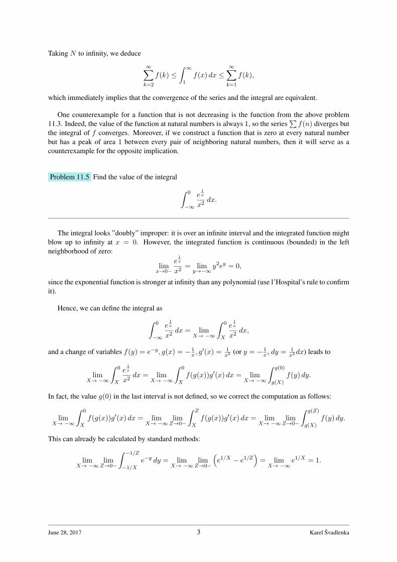
Taking N to infinity, we deduce
∞∑k=2
f(k) ≤∫ ∞
1f(x) dx ≤
∞∑k=1
f(k),
which immediately implies that the convergence of the series and the integral are equivalent.
One counterexample for a function that is not decreasing is the function from the above problem11.3. Indeed, the value of the function at natural numbers is always 1, so the series
∑f(n) diverges but
the integral of f converges. Moreover, if we construct a function that is zero at every natural numberbut has a peak of area 1 between every pair of neighboring natural numbers, then it will serve as acounterexample for the opposite implication.
Problem 11.5 Find the value of the integral ∫ 0
−∞
e1x
x2dx.
The integral looks ”doubly” improper: it is over an infinite interval and the integrated function mightblow up to infinity at x = 0. However, the integrated function is continuous (bounded) in the leftneighborhood of zero:
limx→0−
e1x
x2= lim
y→−∞y2ey = 0,
since the exponential function is stronger at infinity than any polynomial (use l’Hospital’s rule to confirmit).
Hence, we can define the integral as∫ 0
−∞
e1x
x2dx = lim
X→ −∞
∫ 0
X
e1x
x2dx,
and a change of variables f(y) = e−y, g(x) = − 1x , g
′(x) = 1x2 (or y = − 1
x , dy = 1x2dx) leads to
limX→ −∞
∫ 0
X
e1x
x2dx = lim
X→ −∞
∫ 0
Xf(g(x))g′(x) dx = lim
X→ −∞
∫ g(0)
g(X)f(y) dy.
In fact, the value g(0) in the last interval is not defined, so we correct the computation as follows:
limX→ −∞
∫ 0
Xf(g(x))g′(x) dx = lim
X→ −∞lim
Z→0−
∫ Z
Xf(g(x))g′(x) dx = lim
X→ −∞lim
Z→0−
∫ g(Z)
g(X)f(y) dy.
This can already be calculated by standard methods:
limX→ −∞
limZ→0−
∫ −1/Z
−1/Xe−y dy = lim
X→ −∞lim
Z→0−
(e1/X − e1/Z
)= lim
X→ −∞e1/X = 1.
June 28, 2017 3 Karel Svadlenka

Calculus A: Problems with Solutions (Lecture 12)
Problem 12.1 Find the following primitive functions.
(1)∫
1
x2 + xdx
(2)∫
x√1− x4
dx
(3)∫
x3 + x+ 2
x4 + 2x2 + 1dx
(4)∫
secx dx
Each primitive function is determined up to a constant. We omit these constants in the calculationsbelow.
(1) Since 1x2+x
= 1x(x+1) =
1x − 1
1+x , we have∫1
x2 + xdx =
∫ (1
x− 1
1 + x
)dx = ln |x| − ln |1 + x| = ln
∣∣∣∣ x
1 + x
∣∣∣∣ .We use the absolute value to account for the possibility of negative argument, i.e., the primitivefunction of 1
x is lnx + C for x > 0 and ln(−x) for x < 0, which is written compactly byemploying the absolute value.
(2) We use the integration by substitution formula∫f(g(x))g′(x) dx =
∫f(y)dy
with g(x) = x2 and f(y) = 1
2√
1−y2. Then g′(x) = 2x and
∫x√
1− x4dx =
∫f(g(x))g′(x) dx =
∫f(y) dy =
∫1
2√
1− y2dy
=1
2arcsin y =
1
2arcsin(x2).
It is usually easier to use the following formalism instead of the functions f, g above: Set the newvariable y = x2, then dy
dx = 2x and so formally xdx = 12dy, hence replacing x dx by 1
2dy in theintegral and changing x2 to y, we get the integral∫
1
2√
1− y2dy,
which is the same as above.
(3) As x3+x+2x4+2x2+1
= x(x2+1)+2(x2+1)2
= xx2+1
+ 2(x2+1)2
, we can split the integral into two parts:∫x3 + x+ 2
x4 + 2x2 + 1dx =
∫x
x2 + 1dx+
∫2
(x2 + 1)2dx.
Now, the first integral is simple - we use the substitution y = x2 + 1 with dy = 2x dx to get∫x
x2 + 1dx =
∫1
2ydy =
1
2ln y =
1
2ln(x2 + 1),
so it remains to calculate the second integral.
We notice that(
x
x2 + 1
)′=
1− x2
(x2 + 1)2, and thus we can write
∫2
(x2 + 1)2dx =
∫ (1− x2
(x2 + 1)2+
1
x2 + 1
)dx =
x
x2 + 1+ arctanx.
Therefore, the final answer is∫x3 + x+ 2
x4 + 2x2 + 1dx =
1
2ln(x2 + 1) +
x
x2 + 1+ arctanx.
(4) To get a form where substitution can be used, we first rearrange as∫secx dx =
∫cosx
dx =
∫cosx
cos2 xdx =
∫cosx
1− sin2 xdx.
Now we can substitute y = sinx with dy = cosx dx to get∫secx dx =
∫cosx
1− sin2 xdx =
∫1
1− y2dy.
This integral can already be calculated by decomposing into simpler rational functions:∫1
1− y2dy =
1
2
∫ (1
1 + y+
1
1− y
)dy =
1
2(ln |1 + y| − ln |1− y|) = 1
2ln
∣∣∣∣1 + y
1− y
∣∣∣∣ .Hence our integral is ∫
secx dx =1
2ln
∣∣∣∣1 + sinx
1− sinx
∣∣∣∣ ,which can be also written as (after multiplying by 1+sinx
1+sinx )∫secx dx = ln
∣∣∣∣1 + sinx
cosx
∣∣∣∣ = ln |secx+ tanx| .
July 5, 2017 2 Karel Svadlenka

Calculus A: Problems with Solutions (Lecture 13)
Problem 13.1 If the series∑∞
k=1 ak converges, what can you say about the series
∞∑k=1
(a2k + a2k−1) ?
This series converges and has the same sum as∑∞
k=1 ak.
To see this, first write out the new series:
∞∑k=1
(a2k + a2k−1) = (a1 + a2) + (a3 + a4) + (a5 + a6) + · · ·+ (a2K−1 + a2K) + · · · .
Hence we see that the sequence of partial sums of this series is equal to
s2K =
2K∑k=1
ak, K = 1, 2, 3, . . . ,
which is a subsequence of the partial sums of the original series
sK =
K∑k=1
ak.
Since the meaning of ”series∑∞
k=1 ak converges and its sum is S” is that ”the sequence of partial sumssK converges and its limit is S”, we conclude that any subsequence of sK, so also s2K, mustconverge to S, which means that the series
∑∞k=1(a2k + a2k−1) converges and its sum is S.
The key to a correct answer here is to consider first only the partial sums, which are finite andtherefore, we can change order of summation. This will be even more pronounced in problem 13.4.
Problem 13.2 If the series∞∑k=1
(a2k + a2k−1) converges, what can you say about the series∞∑k=1
ak ?
We cannot say anything as the sequence ak = (−1)k, i.e., the sequence −1, 1,−1, 1,−1, . . . shows.Here a2k + a2k−1 = 0 for any k which implies that
∑∞k=1(a2k + a2k−1) converges (it is a sum of
zeros). However, the partial sums sK =∑K
k=1 ak are −1, 0,−1, 0,−1, 0, . . . , which is not a convergentsequence, so the series
∑∞k=1 ak does not converge.

Problem 13.3 Does the series∞∑k=1
ln
(k + 1
k
)converge?
Using the properties of logarithm, we can write the partial sums of this series as
sK =
K∑k=1
ln
(k + 1
k
)=
K∑k=1
(ln(k + 1)− ln k
)and thus it is a telescoping series with partial sums sK = ln(K + 1). When K → ∞, sK diverges toinfinity, hence the given series is divergent.
Problem 13.4 Show that a series∑∞
k=1 ak is absolutely convergent if and only if at least two of theseries
∞∑k=1
ak,∞∑k=1
[ak]+, and
∞∑k=1
[ak]− (1)
converge.
Here, [ak]+ means the positive part of ak, that is, [ak]+ = max0, ak (we are summing only thepositive terms in the series). Similarly, [ak]− = −min0, ak is the negative part.
Since it is an equivalence statement (”if and only if”) we have to prove two implications.
• First, let us prove that if the series∑∞
k=1 ak is absolutely convergent (that is the number S =∑∞k=1 |ak| is finite), then the three series (1) converge.
For the first series∑∞
k=1 ak this is exactly Theorem 3.14 in the textbook. Moreover,
K∑k=1
[ak]+ ≤
K∑k=1
|ak| ≤∞∑k=1
|ak| = S < ∞,
so the sequence of partial sums for the second series in (1) is nondecreasing (because all [ak]+
are nonnegative) and bounded above by S, which means that it must converge (by the monotoneconvergence theorem). For the third series in (1) the argument is completely analogous.
• Next, let us prove that if two of the series (1) converge then∑∞
k=1 ak is absolutely convergent.
Consider, for example, the case when the first two series converge. We denote their sums asfollows:
∞∑k=1
ak = S1,∞∑k=1
[ak]+ = S2.
We notice thatK∑k=1
|ak| =K∑k=1
([ak]
+ − [ak]−)=
K∑k=1
([ak]
+ − (ak − [ak]+))= 2
K∑k=1
[ak]+ −
K∑k=1
ak.
The sequence of partial sums for the series∑∞
k=1 |ak| is nondecreasing because all terms |ak| are non-negative, and moreover it is bounded - to show this we use the above identity in the following way:
K∑k=1
|ak| = 2
K∑k=1
[ak]+ −
K∑k=1
ak ≤ 2
K∑k=1
[ak]+ +
∣∣∣∣∣K∑k=1
ak
∣∣∣∣∣ ≤ 2S2 + |S1| < ∞.
July 11, 2017 2 Karel Svadlenka

An application of the monotone convergence theorem yields the convergence of∑∞
k=1 |ak|.
Other combinations of converging sums in (1) are proved using a similar idea (do it in detail).
Problem 13.5 For which values of x does the following series converge?
∞∑n=2
xn
log n
We will consider several cases for x and check the convergence in each case by different methods(just to show how to use them). If there is no log n in each term, the boundary value for convergencewould be x = ±1. Since log n does not have much strength comparing to the exponential growth of xn,we try to divide the interval for x in the same way.
1. x > 1
We use for example the root test (3.30 in the textbook):
limn→∞
n
√xn
log n= lim
n→∞
xn√log n
≥ limn→∞
xn√n= x > 1,
so the series diverges. Here we used the fact that log n < n for n ≥ 2 and that limn→∞ n√n = 1.
2. x = 1
In this case we have the series∞∑n=2
1
log n.
We can use the comparison test II (3.20 in the textbook) with harmonic series:
1
n<
1
log nand
∞∑n=2
1
ndiverges,
so the above series also diverges.
Note that the root test would not give us any information here because the limit would be 1.
3. x ∈ [0, 1)
Let us use the ratio test (3.28 in the textbook):
limn→∞
xn+1
log(n+ 1)
log n
xn= lim
n→∞x
log n
log(n+ 1)
= limn→∞
xlog(n+ 1) + log n
n+1
log(n+ 1)
= limn→∞
x
(1 +
log nn+1
log(n+ 1)
)= x < 1,
so the series converges.
4. x ∈ (−1, 0)
In this case, the series of absolute values∑∞
n=2 |xn/ log n| is the same as in the previous case, sothe series converges absolutely.
July 11, 2017 3 Karel Svadlenka

5. x = −1
Here the series becomes∞∑n=2
(−1)n
log n,
so we can use the alternating series test (3.43 in the textbook) to say that the series converges.However, it does not converge absolutely since the series
∑∞n=2
1logn diverges.
6. x < −1
We can use the trivial test:limn→∞
xn
log n
does not exist (because the terms change signs and the subsequence x2n
log(2n) diverges to infinity),so the series cannot converge.
In summary, the series converges absolutely for x ∈ (−1, 1), converges nonabsolutely for x = −1and diverges otherwise.
Problem 13.6 Determine the values of s, for which the series
∞∑n=2
1
n(log n)s
converges.
If we try to use the root test or ratio test, we end up with the indecisive limit 1, so these tests cannotbe used.
For s ≤ 0, we can use the comparison with harmonic series:
1
n(log n)s≥ 1
nand
∞∑n=1
1
ndiverges,
so our series diverges for s ≤ 0.
For general s, the integral test (3.35 in the textbook) works: if s = 1 then
limX→∞
∫ X
2
1
x(log x)sdx = lim
X→∞
∫ logX
log 2
1
ysdy = lim
X→∞
[− 1
s− 1
1
ys−1
]logXlog 2
= limX→∞
− 1
s− 1
[1
ys−1
]Xlog 2
=1
s− 1
(1
(log 2)s−1− lim
X→∞
1
Xs−1
)We have used the change of variables y = log x. We see that the limit of the integral is finite if and onlyif s > 1.
In the special case when s = 1, we have
limX→∞
∫ X
2
1
x log xdx = lim
X→∞
∫ logX
log 2
1
ydy = lim
X→∞[log y]logXlog 2 = lim
X→∞log(logX)− log(log 2)
In this case, the limit becomes infinite, so the series does not converge.
July 11, 2017 4 Karel Svadlenka

REFERENCES
In summary, our series converges if and only if s > 1.
(See also http://math.feld.cvut.cz/mt/txte/2/txe3ec2.htm for more examples of testing convergence ofseries.)
Additional Problems
Problem 1 ([2], p.489) Decide whether each of the following series is convergent or divergent:
(1)∞∑n=1
sinnθ
n2, θ ∈ R (2) 1− 1
3+
1
5− 1
7+ · · · (3) 1− 1
2+
2
3− 1
3+
2
4− 1
4+
2
5− 1
5+ · · ·
(4)∞∑n=1
(−1)nlog n
n(5)
∞∑n=2
13√n2 − 1
(6)∞∑n=1
13√n2 + 1
(7)∞∑n=1
n2
n!(8)
∞∑n=1
log n
n
(9)∞∑n=2
1
log n(10)
∞∑n=2
1
(log n)k, k ∈ N (11)
∞∑n=2
1
(log n)n(12)
∞∑n=2
(−1)n1
(log n)n
(13)∞∑n=1
n2
n3 + 1(14)
∞∑n=1
sin1
n(15)
∞∑n=2
1
n log n(16)
∞∑n=2
1
n(log n)2
(17)∞∑n=2
1
n2(log n)(18)
∞∑n=1
n!
nn(19)
∞∑n=1
2nn!
nn(20)
∞∑n=1
3nn!
nn.
Problem 2 ([1], p.413) Test the following series for convergence and absolute convergence:
(1)∞∑n=1
(−1)nn
3n− 2(2)
∞∑n=1
n!
2n(3)
∞∑n=1
ne−n (4)∞∑n=1
1√1 + n3
(5)∞∑n=1
(−1)n−1 n
n2 + 1(6)
∞∑n=3
(−1)n−1 1
log(log n)(7)
∞∑n=1
nq
1 + nq, q ∈ R
(8)∞∑n=1
rn
1 + r2n, r ∈ R (9)
∞∑n=1
(−1)n−1 sin1
np, p ∈ R (10)
∞∑n=1
cos(nθ)√n
.
References
[1] S.R. Ghorpade, B.V. Limaye: A Course in Calculus and Real Analysis, Springer, 2006.
[2] M. Spivak: Calculus, Publish or Perish, 2008.
July 11, 2017 5 Karel Svadlenka

Calculus B: Problems with Solutions (Lecture 1)
Problem 1.1 Let
fn(x) =sinnx√
n.
Show that limn→∞ fn(x) = 0 but limn→∞ f ′n(0) = ∞.
The pointwise limit of the sequence of functions can be easily obtained from the squeeze theorem.Notice that because sinx is bounded above by 1 and below by −1, we have that
− 1√n≤ sinnx√
n≤ 1√
n.
Since both expressions − 1√n
and 1√n
tend to 0 as n → ∞, the quantity fn(x) must also tend to 0 forevery x ∈ R, by the squeeze theorem.
We computef ′n(0) =
n cosnx√n
∣∣∣x=0
=√n cosnx
∣∣∣x=0
=√n.
Therefore, obviously f ′n(0) → ∞ as n → ∞.
The reason why we cannot interchange limit and differentiation in this case is that the assumption ofTheorem 9.34 that ”the sequence f ′
n(x) converges uniformly on [a, b]” is not satisfied for any intervalaround 0. Indeed, f ′
n(x) =√n cosnx does not even converge pointwise for any neighborhood of 0.
Problem 1.2 Examine the uniform limiting behavior of the sequence of functions
fn(x) = x2e−nx.
On what sets can you determine uniform convergence?
First, we check the pointwise convergence to find the limit function, and then investigate if the con-vergence is uniform.
We see that for x < 0 the exponent −nx is positive and increasing to infinity for n → ∞, so thatfn(x) → ∞. If x = 0 then fn(0) = 0 for all n so that the limit is 0. If x > 0 then the exponent −nxis negative and decreases to −∞ as n → ∞, which implies fn(x) → 0. (To be precise we should showit from definition, that is for any given ε find N so that x2e−nx < ε when n ≥ N . But that is easy, justtake N > (2 lnx− ln ε)/x. The same for the case x < 0.) We conclude
limn→∞
fn(x) =
∞ if x < 00 if x ≥ 0
.
Since ∞ is not a number and therefore the limit function is not defined for x < 0, we investigateuniform convergence on the interval [0,∞) only. The graph of the function fn(x) looks like in thefollowing figure (here n = 3).

0 0.5 1 1.5 2 2.5 3 3.5 40
0.01
0.02
0.03
0.04
0.05
0.06
0.07
It is easy to check that it is increasing on x ∈ (0, 2n) and decreasing on ( 2n ,∞), where the maximum
is attained at x = 2n and is equal to 4
n2 e−2.
In order for the function to converge uniformly to the zero function on [0,∞), it is necessary that thevalues of fn are smaller than any given ε > 0 if n is large enough (that is, if n ≥ N for some N ). In thiscase this is obviously true because the maximum of fn on [0,∞) is equal to 4
n2 e−2, which decreases to
0 when n → ∞. Hence, given ε > 0, we set N > 2/(e√ε) and then |fn(x) − 0| < ε for any n ≥ N .
This shows that fn(x) converges uniformly to f(x) = 0 on the interval [0,∞).
We could show it also by the equivalent definition using sup as follows:
limn→∞
supx∈[0,∞)
|fn(x)− f(x)| = limn→∞
supx∈[0,∞)
|fn(x)| = limn→∞
4
n2e−2 = 0.
Problem 1.3 Prove that fn → f converges uniformly on D if and only if
limn→∞
supx∈D
|fn(x)− f(x)| = 0. (1)
First assume that (1) holds. We will show that fn converges to f according to Definition 9.9. Letε > 0. Then according to the definition of the limit in (1), we can find N , so that
supx∈D
|fn(x)− f(x)| < ε when n ≥ N.
But the above inequality means (by the definition of supremum) that
|fn(x)− f(x)| < ε for all x ∈ D if n ≥ N.
This is exactly the statement in Definition 9.9.
On the contrary, assume that fn converges uniformly to f on D according to Definition 9.9. Letε > 0. Then there is N such that
|fn(x)− f(x)| < ε/2 for all x ∈ D and all n ≥ N.
This means that for every n ≥ N we have
supx∈D
|fn(x)− f(x)| ≤ ε/2 < ε.
October 4, 2017 2 Karel Svadlenka

But this is the definition of the limit in identity (1) (i.e., for every ε > 0 we could find N so that etc. -this is the definition of limit).
Problem 1.4 Verify that the geometric series∑∞
k=0 xk, which converges pointwise on (−1, 1), does
not converge uniformly there.
The geometric series has the sum 11−x for |x| < 1, which shows that it converges pointwise on
(−1, 1). In Example 9.15 it is shown that the series converges uniformly on any interval [0, η], where0 < η < 1. In the same way we could show that it converges uniformly on any interval [−η, η], where0 < η < 1.
Let us show that it does not converge uniformly on (−1, 1). This means that the sequence of partialsums
Sn(x) =
n∑k=0
xk =1− xn+1
1− x
does not converge uniformly to the function S(x) = 11−x . To prove it, we will use the equivalent
definition of uniform convergence from Problem 1.3. That is the series converges uniformly if and onlyif
limn→∞
supx∈(−1,1)
|Sn(x)− S(x)| = 0. (2)
We compute the difference in absolute values:
|Sn(x)− S(x)| =∣∣∣∣1− xn+1
1− x− 1
1− x
∣∣∣∣ = |x|n+1
1− x.
Checking the supremum on (−1, 1), we find
supx∈(−1,1)
|Sn(x)− S(x)| = supx∈(−1,1)
|x|n+1
1− x= ∞,
since the function |x|n+1/(1− x) diverges to ∞ when x → 1−. Hence the limit in (2) cannot be 0 andthe series does not converge uniformly on (−1, 1).
The problem here is with the point x = 1 because there |Sn(x)− S(x)| diverges to ∞. One can seefrom the above calculation that if we restrict ourselves to an interval [−η, η] with 0 < η < 1, then weget uniform convergence because
|Sn(x)− S(x)| ≤ |η|n+1
1− η→ 0 as n → ∞.
Problem 1.5 Let fn be a sequence of functions each of which is uniformly continuous on an openinterval (a, b). If fn → f uniformly on (a, b) can you conclude that f is also uniformly continuous on(a, b)?
Yes. We can show that for any given ε > 0, we can find δ > 0, so that
|f(x1)− f(x2)| < ε whenever |x1 − x2| < δ and x1, x2 ∈ (a, b)
in the following way.
October 4, 2017 3 Karel Svadlenka

Let ε > 0 and from the definition of uniform convergence of fn find N such that
|fn(x)− f(x)| < ε
3for every n ≥ N and all x ∈ (a, b).
Moreover, from the definition of uniform continuity of fN find δ such that
|fN (x1)− fN (x2)| <ε
3whenever |x1 − x2| < δ and x1, x2 ∈ (a, b).
Then, for any x1, x2 ∈ (a, b) such that |x1 − x2| < δ we have
|f(x1)− f(x2)| ≤ |f(x1)− fN (x1)|+ |fN (x1)− fN (x2)|+ |fN (x2)− f(x2)| ≤ε
3+
ε
3+
ε
3= ε.
This completes the proof of uniform continuity of f .
Problem 1.6 Prove that
limn→∞
∫ π
π2
sinnx
nxdx = 0.
We can use Theorem 9.26 on the sequence of functions
fn(x) =sinnx
nx, x ∈ [π2 , π].
To this end, we just need to check the assumptions of the theorem:
• limn→∞
fn(x) = f(x) for all x ∈ [π2 , π].
If we fix any x ∈ [π2 , π], we compute
f(x) = limn→∞
fn(x) = limn→∞
sinnx
nx= 0.
(This limit can be computed by the squeeze theorem.)
• Each function fn is continuous on [π2 , π].
This is obvious, since sin is continuous and the denominator never becomes zero on the interval[π2 , π].
• The convergence of fn is uniform on [π2 , π].
We use the equivalent definition from solved problem 1.3. First we estimate
0 ≤ supx∈[π
2,π]
∣∣∣∣sinnxnx
∣∣∣∣ ≤ supx∈[π
2,π]
1
nx=
1
nπ2
.
Since we have sandwiched the supremum between 0 and 2nπ , which both tend to 0 as n → ∞, we
conclude that
limn→∞
supx∈[π
2,π]
∣∣∣∣sinnxnx
∣∣∣∣ = 0,
which means that the convergence is uniform on [π2 , π].
October 4, 2017 4 Karel Svadlenka

Since all the assumptions of the theorem are fulfilled, we conclude
limn→∞
∫ π
π2
fn(x) dx =
∫ π
π2
f(x) dx =
∫ π
π2
0 dx = 0,
which implies
limn→∞
∫ π
π2
sinnx
nxdx = 0.
Note that it would be very difficult to calculate the integral without first interchanging the order of limitand integration.
Problem 1.7 Show that if fn → f uniformly on [a, b] and each fn is continuous then the sequence offunctions
Fn(x) =
∫ x
afn(t) dt
also converges uniformly on [a, b].
Let ε > 0. From the uniform convergence of fn to f , we can find N such that
|fn(t)− f(t)| < ε
b− afor every t ∈ [a, b]. (3)
DefineF (x) =
∫ x
af(t) dt.
This integral is well-defined because f is continuous on [a, b] (it is a uniform limit of a sequence ofcontinuous functions, so it must be continuous).
Then, if x is any point in [a, b] and n ≥ N , we have
|Fn(x)− F (x)| =∣∣∣∣∫ x
afn(t) dt−
∫ x
af(t) dt
∣∣∣∣ = ∣∣∣∣∫ x
a(fn(t)− f(t)) dt
∣∣∣∣ ≤ ∫ x
a|fn(t)− f(t)| dt.
In the last estimate we used the absolute property 8.7 of integral. Thus by (3),
|Fn(x)− F (x)| ≤∫ x
a|fn(t)− f(t)| dt ≤
∫ x
a
ε
b− adt ≤
∫ b
a
ε
b− adt =
ε
b− a(b− a) = ε.
This shows, by definition, the uniform convergence of Fn to F on [a, b].
Problem 1.8 Can the sequence of functions fn(x) = sinnxn3 be differentiated term by term? How about
the series∑∞
k=1sin kxk3
?
For the sequence, we use Theorem 9.34, which requires us to check two main conditions:
• f ′n converges to uniformly to some function g
Notice that Theorem 9.34 requires a bounded interval [a, b] so we select any R > 0 and check theuniform convergence on [−R,R]. We easily find that g(x) = 0 and so we calculate
limn→∞
supx∈[−R,R]
|f ′n(x)− g(x)| = lim
n→∞sup
x∈[−R,R]
∣∣∣cosnxn2
∣∣∣ ≤ limn→∞
supx∈[−R,R]
1
n2= lim
n→∞
1
n2= 0.
October 4, 2017 5 Karel Svadlenka

Thus f ′n converges uniformly to the zero constant function (we use the squeeze theorem to show
that the above limit is 0).
• fn converge pointwise to some function f
This is easy: pick any x ∈ [−R,R] and set f(x) = 0, then
limn→∞
|fn(x)− f(x)| = limn→∞
| sinnx|n3
≤ limn→∞
1
n3= 0.
Therefore, fn converge pointwise to the zero function f(x) = 0 on [−R,R].
Theorem 9.34 now implies that we can switch the order of limit and differentiation for the sequencefn(x) on any bounded interval, which is the same as saying that the sequence can be differentiatedterm by term.
Now, let us look at the series∑∞
k=1sin kxk3
. Note that even if the sequence fn converges uniformly,that does not imply that
∑fk(x) converges uniformly, since we are ”adding up” the functions fk (e.g.,
fn(x) = 1/n converges uniformly to 0 but∑
1/n = ∞).
To get the answer, we use Corollary 9.35, which again requires us to check two basic assumptions(we check them again on any interval [−R,R]):
•∑
f ′k converges uniformly to some function g
We use the M -test (Theorem 9.16). Setting Mk = 1/k2 we find
|f ′k(x)| =
| cos kx|k2
≤ Mk.
Moreover,∞∑k=1
Mk =
∞∑k=1
1
k2< ∞
converges (p-harmonic series with p = 2). Hence, the M -test implies that∑
f ′k converges uni-
formly on [−R,R].
•∑
fk converge pointwise to some function f
This is again easier than the first assumption: pick any x ∈ [−R,R], then∣∣∣∣∣∞∑k=1
fk(x)
∣∣∣∣∣ ≤∞∑k=1
| sin kx|k3
≤∞∑k=1
1
k3< ∞.
Therefore,∑
fk converges pointwise on [−R,R].
By Corollary 9.35, we can switch the order of summation and differentiation.
October 4, 2017 6 Karel Svadlenka

Problem 1.9 Compute the limit
limn→∞
∫ 1
0
e−nt
√tdt.
Since we want to apply Theorem 9.33, we first use a change of variables to transform the improperintegral of a discontinuous function on a bounded interval to an integral of a continuous function on anunbounded interval. Set x = 1/
√t, then t = 1/x2 and dt = −2/x3dx, and we get∫ 1
0
e−nt
√tdt =
∫ 1
∞
e−n/x2
1x
−2
x3dx = 2
∫ ∞
1
e−n/x2
x2dx.
We see that we are in the situation of Theorem 9.33 with a = 1 and
fn(x) =1
x2e−n/x2
, x ∈ [1,∞).
Now, to apply the theorem and change the order of limit and integration, we have to check thefollowing assumptions:
• fn converge uniformly to a function f on any [1, b], b > 1
We expect f(x) = 0, so let us compute
limn→∞
supx∈[1,b]
|fn(x)− f(x)| = limn→∞
supx∈[1,b]
1
x2e−n/x2
.
The surest way to find the above supremum is to investigate the extrema of the functions fn(x).We find that
f ′n(x) =
−2
x3e−n/x2
+1
x2e−n/x2 2n
x3=
2
x3e−n/x2
(−1 + nx2 ).
The derivative is positive on [1,√n) and negative on (
√n,∞), so the maximum is attained at
x =√n, where fn(
√n) = 1
en (if b is less than√n then the maximum is even smaller than this
value). Hence,
limn→∞
supx∈[1,b]
|fn(x)− f(x)| = limn→∞
1
en= 0,
and we conclude that the sequence converges uniformly on [1, b] to f(x) = 0 for any b > 1.
• there is an integrable dominating function g(x) for fn(x)
We have to find g so that |fn(x) ≤ g(x) for all x ∈ [1,∞) and such that g is integrable on (1,∞).Note that g must be independent of n (that is, one function g has to dominate all the functions inthe sequence fn). Since e−n/x2 ≤ 1 for x ∈ [1,∞), we can try
g(x) =1
x2.
By direct computation we check that this function is integrable (∫∞1
1x2 dx = 1).
All assumptions of Theorem 9.33 are satisfied and we conclude
limn→∞
∫ 1
0
e−nt
√tdt = lim
n→∞2
∫ ∞
1
e−n/x2
x2dx = 2
∫ ∞
1limn→∞
e−n/x2
x2dx = 2
∫ ∞
10 dx = 0.
October 4, 2017 7 Karel Svadlenka

Calculus B: Problems with Solutions (Lecture 2)
There are no solved problems for this lecture since they are included in the material for previous lecture- see ”Problems with Solutions (Lecture 1)”.

Calculus B: Problems with Solutions (Lecture 3)
Problem 3.1 Find the radius of convergence for the series
∞∑k=0
k!xk.
Since it is not so easy to calculate the limit of k√k!, we try to use the ratio test instead of the root test.
Setting ak = k!xk we compute
limk→∞
∣∣∣∣ak+1
ak
∣∣∣∣ = limk→∞
∣∣∣∣(k + 1)!xk+1
k!xk
∣∣∣∣ = limk→∞
(k + 1)|x| = ∞ for any x = 0.
Therefore, by the ratio test, the series converges absolutely only for x = 0. This gives us informationonly on absolute convergence since the ratio test applies only to series with positive terms (we haveapplied it to the series of absolute values). However, since we know that the interval of convergence forthe power series is an interval centered at x = 0, and we have just shown that the series diverges for allpositive x, we conclude that the radius of convergence is R = 0.
Another proof uses the trivial test noticing that
limk→∞
k!xk
is either ∞ (when x > 0) or does not exist (when x < 0) (why?). In either case the trivial test says thatthe series cannot converge and we immediately get R = 0.
Problem 3.2 If the limit
limk→∞
∣∣∣∣ akak+1
∣∣∣∣exists or equals ∞, then show that it gives the radius of convergence of the power series
∑∞k=0 akx
k.Give an example of a power series
∑∞k=0 akx
k for which the radius of convergence R satisfies
R =1
limk→∞k√
|ak|
but
limk→∞
∣∣∣∣ akak+1
∣∣∣∣does not exist.
We use the inequalities (proved later)
lim infk→∞
∣∣∣∣ak+1
ak
∣∣∣∣ ≤ lim infk→∞
k√
|ak| ≤ lim supk→∞
k√
|ak| ≤ lim supk→∞
∣∣∣∣ak+1
ak
∣∣∣∣ .

If the limit
limk→∞
∣∣∣∣ akak+1
∣∣∣∣exists and is not equal to 0 (and also is not ∞), then the limit
limk→∞
∣∣∣∣ak+1
ak
∣∣∣∣ = 1
limk→∞
∣∣∣ akak+1
∣∣∣also exists and is neither 0 nor ∞, which means that lim inf and lim sup of this sequence are equal (andequal to the limit), so all the four terms in the above chain of inequalities must be equal. Hence, thelim inf and lim sup of the sequence k
√|ak| are equal, which means that the limit of this sequence
exists and equals the lim inf and lim sup. We conclude
limk→∞
∣∣∣∣ akak+1
∣∣∣∣ = 1
limk→∞k√
|ak|.
The case of zero or infinite limit are similar. For example, if the limit of |ak|/|ak+1| is 0, then thelimit of |ak+1|/|ak| is infinity and the lim inf is also ∞ and all the terms in the chain of inequalitiesare ∞ (because they are defined).
To find the required counterexample, set
ak =
1 when k is oddk when k is even
,
that is, ak = 1, 2, 1, 4, 1, 6, 1, 8, 1, 10, 1, . . . . Since
k√1 ≤ k
√ak ≤ k
√k,
we see by the squeeze theorem thatlimk→∞
k√ak = 1.
However, akak+1
=
1
2, 2,
1
4, 4,
1
6, 6, . . . ,
so the limit of this sequence does not exist.
It remains to prove the chain of inequalities. We prove only the last inequality
lim supk→∞
k√
|ak| ≤ lim supk→∞
∣∣∣∣ak+1
ak
∣∣∣∣ , (1)
the first inequality being analogous and the second one following from Theorem 2.46. Let β be anynumber larger than lim supk→∞
∣∣∣ak+1
ak
∣∣∣. Then, by the definition of lim sup, there exists N such that
|ak+1||ak|
< β for every k ≥ N.
This implies
|aN+1| < β|aN | ⇒ |aN+k| < βk|aN | ⇒ N+k√
|aN+k| < β N+k
√|aN |βN
.
Keeping N fixed and taking k → ∞ in the last inequality, we get
lim supk→∞
k√
|ak| = lim supk→∞
N+k√
|aN+k| ≤ β.
October 18, 2017 2 Karel Svadlenka

This means that lim supk→∞k√
|ak| is less than or equal to any number which is greater than
lim supk→∞
∣∣∣ak+1
ak
∣∣∣, hence the inequality (1) is proved.
Problem 3.3 If the coefficients ak of a power series∑∞
k=0 akxk form a bounded sequence, show that
the radius of convergence is at least 1.
If the radius of convergence R of the series is ∞, then the statement is true and there is nothing toshow, so let us assume that R is finite. Since ak is bounded, there exists M > 0 such that |ak| ≤ Mfor all k = 0, 1, 2, . . . . This implies
k√
|ak| ≤k√M ⇒ lim sup
k→∞
k√
|ak| ≤ lim supk→∞
k√M ⇒ 1
lim supk→∞k√
|ak|≥ 1
lim supk→∞k√M
.
But we know (see Example 2.33) that limk→∞k√M = 1 for any positive M , so the last inequality above
says that R ≥ 1, which is what we wanted to prove.
Problem 3.4 Show that if∑∞
k=0 akxk converges uniformly on an interval (−r, r), then it must in fact
converge uniformly on [−r, r].
Let ε > 0 be given. If the power series converges uniformly on (−r, r), then according to the Cauchycriterion (Theorem 9.14), we see that there is N such that∣∣∣∣∣
n∑k=m
akxk
∣∣∣∣∣ < ε
2for any m,n ≥ N and any x ∈ (−r, r).
Fix any m,n ≥ N . Then the left-hand side of the above inequality is a continuous function in x. Thus,taking the limit as x → r− and x → −r+, respectively, we deduce∣∣∣∣∣
n∑k=m
akrk
∣∣∣∣∣ ≤ ε
2< ε,
∣∣∣∣∣n∑
k=m
ak(−r)k
∣∣∣∣∣ ≤ ε
2< ε.
This means that ∣∣∣∣∣n∑
k=m
akxk
∣∣∣∣∣ < ε for any m,n ≥ N and any x ∈ [−r, r],
and this, in turn, means by the Cauchy criterion that the series converges uniformly on [−r, r].
October 18, 2017 3 Karel Svadlenka

Calculus B: Problems with Solutions (Lecture 4)
Problem 4.1 Obtain power series expansion about x = 0 forx
1 + x2
and find the largest interval where this expansion is valid.
Since1
1 + x2= 1− x2 + x4 − x6 + · · · =
∞∑k=0
(−1)kx2k for x ∈ (−1, 1)
by the sum of geometric series, we formally have
x
1 + x2= x− x3 + x5 − x7 + · · · =
∞∑k=0
(−1)kx2k+1
but we have to check for what values of x this formula is valid.
Since the coefficients ak of this power series are either 0 or 1 or −1 (when we write the series in theform
∑∞k=0 akx
k), we have lim supk→∞k√
|ak| = 1 and get from the formula for radius of convergencethat
R =1
lim supk→∞k√
|ak|= 1,
so the formula is valid for x ∈ (−1, 1). It is easy to check that it is not valid for the endpoints x = 1 andx = −1.
We can also use the arguments in Section 10.6, which say that the radius of convergence of the seriesfor x
1+x2 is at least the smaller value of the radius of convergence for x (R1 = ∞) and of the radius ofconvergence of the series for 1
1+x2 (R2 = 1).
Problem 4.2 Let
f(x) =
0, if x = 0
e−1/x2, if x = 0
Prove that f is infinitely differentiable on the real line. Show that f (k)(0) = 0 for all k ∈ N. Explainwhy the Taylor series for f about x = 0 does not represent f in any neighborhood of zero.
The function f is obviously infinitely differentiable on the interval (−∞, 0) and on the interval(0,∞) because the derivatives of f in these intervals
f ′(x) =2
x3e−1/x2
, f ′′(x) =
(− 6
x4+
4
x6
)e−1/x2
, etc.
are functions of the type
f (m)(x) =
(n∑
k=1
akxk
)e−1/x2
,

which are continuous on any interval not including x = 0.
It remains to check the differentiability at x = 0. We show by induction that f (m)(0) = 0 for allm ∈ N ∪ 0. For m = 0 this holds by the definition of the function f . If f (m)(0) = 0, let us computef (m+1)(0):
f (m+1)(0) = limx→0
f (m)(x)− f (m)(0)
x− 0=
(n∑
k=1
akxk+1
)e−1/x2
.
If we show that limx→01xk e
−1/x2= 0 for any k = 1, 2, . . . , then the above limit will be zero and we are
done. But this limit can be calculated by squeeze theorem and L’Hospital’s rule from
limx→0
1
|x|ke−1/x2
= limy→∞
yk
ey2= 0.
Since all derivatives of f at x = 0 vanish, the Taylor series about the point x = 0 would be the zeroseries. However, since the function is nonzero (positive) in any neighborhood of the origin x = 0, theTaylor series cannot represent f on any neighborhood of x = 0.
Problem 4.3 Verify that the function cosx2 is analytic at x = 0, and write its Taylor series about x = 0.
We can use Theorem 10.33. in particular cosx2 is a composition of two functions f(x) = cosx andg(x) = x2, where g(x) is a polynomial, so it can be considered as a power series centered at x0 = 0 andwith its first term equal to C = 0:
g(x) = 0 + 0x+ x2 + 0x3 + · · · .
If we expand f(x) about the point C = 0 as follows
cosx = 1− x2
2!+
x4
4!− x6
6!+ · · · =
∞∑k=0
(−1)kx2k
(2k)!
(we know from the textbook that cosx is analytic on R and that the above expansion holds for everyx ∈ R), Theorem 10.33 asserts that the power series for the composition f(g(x)), obtained by insertingthe expansion of g into the expansion of f , has a positive radius of convergence R (actually, both fand g have infinite radius of convergence, and so does f(g(x))). This means that the function cosx2 isanalytic in a neighborhood of the origin (since it can be represented by a power series in (−R,R)) andin this neighborhood
cosx2 = 1− (x2)2
2!+
(x2)4
4!− (x2)6
6!+ · · · = 1− x4
2!+
x8
4!− x12
6!+ · · · =
∞∑k=0
(−1)kx4k
(2k)!.
October 25, 2017 2 Karel Svadlenka

Problem 4.4 Find first four terms of the series expansion of tanx about x = 0 using the followingthree methods:
• long division (quotient of series),
• product of series,
• usual formula for Taylor series.
The power series for sinx and cosx are
sinx = x− x3
3!+
x5
5!− x7
7!+ · · · =
∞∑k=0
(−1)kx2k+1
(2k + 1)!
cosx = 1− x2
2!+
x4
4!− x6
6!+ · · · =
∞∑k=0
(−1)kx2k
(2k)!,
where these expansions are valid for all x ∈ R. We briefly describe the three methods to obtain theTaylor series for
tanx = c0 + c1x+ c2x2 + c3x
3 + · · · .Since we are required to find the first four terms, it is enough to calculate c0, c1, c2, c3.
• quotient of series (see Section 10.6.1):
Theorem 10.32 says that the quotient series for sinx/ cosx is valid in some neighborhood of zero.We can find the coefficients by division or from the equation
(c0 + c1x+ c2x2 + c3x
3 + · · · )(1− x2
2!+
x4
4!− · · ·
)= x− x3
3!+
x5
5!− · · · .
Multiplying out the left-hand side, we get
c0 + c1x+(−c0
2+ c2
)x2 +
(−c1
2+ c3
)x3 + · · · = x− x3
3!+ · · · .
Comparing the coefficients we immediately see that c0 = c2 = 0, c1 = 1, c3 =13 . Hence
tanx = x+1
3x3 + · · · .
• product of series (see Section 10.6):
We take the function tanx as the product of functions sinx and 1cosx , write the power series for
these two functions and multiply them. Since both the functions are analytical in the neighborhoodof 0, the power series obtained by multiplication will also be valid in some neighborhood of zero.The derivatives of 1
cosx are(1
cosx
)′=
sinx
cos2 x,
(1
cosx
)′′=
1 + sin2 x
cos3 x,
(1
cosx
)′′′=
sinx(5 + sin2 x)
cos4 x.
Therefore,(
1cosx
)′ |x=0 = 0,(
1cosx
)′′ |x=0 = 1,(
1cosx
)′′′ |x=0 = 0, and in a neighborhood ofx = 0,
1
cosx= 1 +
1
2x2 + 0x3 + · · · .
Multiplying this expansion with the expansion for sinx we have
tanx =
(1 +
1
2x2 + · · ·
)(x− x3
3!+ · · ·
)= x+
1
3x3 + · · · .
October 25, 2017 3 Karel Svadlenka

• usual formula for Taylor series:
The first three derivatives of tanx are
(tanx)′ =1
cos2 x, (tanx)′′ =
2 sinx
cos3 x, (tanx)′′′ =
2(1 + 2 sin2 x)
cos4 x,
so we obtain tan 0 = 0, tan′(0) = 1, tan′′(0) = 0, tan′′′(0) = 2. Plugging these values intothe formula for Taylor series, we have
tanx = tan 0 + tan′(0)x+tan′′(0)
2!x2 +
tan′′′(0)
3!x3 + · · · = x+
1
3x3 + · · · .
October 25, 2017 4 Karel Svadlenka
Calculus B: Problems with Solutions (Lecture 5)
Problem 5.1 Show that∥x∥∞ = max(|x1|, |x2|, . . . , |xn|)
is a norm (i.e., that it has the properties listed in Theorem 11.6 in the textbook).
We check the properties (i)–(iii) one by one.
(i) ∥x∥∞ ≥ 0 and ∥x∥∞ = 0 if and only if x = 0
Since ∥x∥∞ is the maximum of a finite number of nonnegative numbers, it must be itselfnonnegative. Hence, ∥x∥∞ ≥ 0.
Now, if x = 0 then obviously ∥x∥∞ = max(0, . . . , 0) = 0. On the other hand, if ∥x∥∞ = 0then the maximum of n nonnegative numbers |x1|, . . . , |xn| being zero means that all thenumbers have to be zero. Therefore, x = 0.
(ii) ∥αx∥∞ = |α| ∥x∥∞, α ∈ R
∥αx∥∞ = max(|αx1|, |αx2|, . . . , |αxn|) = max(|α||x1|, |α||x2|, . . . , |α||xn|)= |α|max(|x1|, |x2|, . . . , |xn|) = |α| ∥x∥∞.
(iii) ∥x+ y∥∞ ≤ ∥x∥∞ + ∥y∥∞
∥x+ y∥∞ = max(|x1 + y1|, |x2 + y2|, . . . , |xn + yn|)≤ max(|x1|+ |y1|, |x2|+ |y2|, . . . , |xn|+ |yn|)≤ max(|x1|, |x2|, . . . , |xn|) + max(|y1|, |y2|, . . . , |yn|)= ∥x∥∞ + ∥y∥∞,
where we used the triangle inequality for real numbers in the first inequality and the factthat
max(a1 + b1, a2 + b2) ≤ max(a1, a2) + max(b1, b2)
(which can be proved by checking all the possible cases) in the second inequality.
Problem 5.2 Prove that a set E ⊂ Rn is closed if and only if it contains all its accumulationpoints.
We have defined a closed set E as a set for which Rn \ E is an open set.
• Assume that E is closed and that there is an accumulation point x0 of E that does notbelong to E. Then x0 ∈ Rn \E and also there exists a sequence of points xk ⊂ E suchthat xk → x0. Therefore, for any ε > 0 there is a point xK such that ∥xK − x0∥ < ε.This means that in any ball B(x0, ε) centered at x0 there is some point belonging to E.However, this is a contradiction with Rn \E being open (for x0 ∈ Rn \E there must exista radius r > 0 so that B(x0, r) ⊂ Rn \ E but we have proved above that each such ballcontains a point from E, that is, a point which is not in Rn \ E), which proves the firstimplication.

• To prove the converse implication assume that E contains all its accumulation points butis not closed. This implies that F = Rn \ E is not open, so there is a point x0 ∈ Fsuch that for any n ∈ N there exists a point xn ∈ B(x0,
1n), which does not belong to F
(and thus belongs to E). Then the sequence xn is contained in E and converges to x0
(because ∥xn−x0∥ ≤ 1n). Hence, x0 is an accumulation point of E but it does not belong
to E, which is a contradiction, and the second implication is proved.
Problem 5.3 Let xk be a sequence in Rn and let α ∈ R. If limk→∞ xk = x, show that then
limk→∞
(αxk) = αx.
Let ε > 0 and assume that α = 0 (since otherwise there is nothing to prove). We use thesecond property of the norm to find
∥(αxk)− (αx)∥ = ∥α(xk − x)∥ = |α| ∥xk − x∥.
Since xk → x, for ε = ε/|α| there exists K such that
∥xk − x∥ < ε for any k ≥ K.
From the above estimate we then obtain
∥(αxk)− (αx)∥ = |α| ∥xk − x∥ ≤ |α|ε = ε for every k ≥ K,
which is what we had to prove.
Problem 5.4 Define the norm ∥x∥1 = |x1| + · · · + |xn|. Show that for a sequence xk in Rn
the following holds:
limk→∞
xk = x if and only if ∥xk − x∥1 → 0 as k → ∞.
This means that convergence does not depend on which of the norms ∥ · ∥ (euclidean norm) or∥ · ∥1 we use.
We have
∥xk − x∥ =√
|xk1 − x1|2 + · · ·+ |xkn − xn|2 ≤ |xk1 − x1|+ · · ·+ |xkn − xn|,
which can be rewritten as0 ≤ ∥xk − x∥ ≤ ∥xk − x∥1.
Hence, if ∥xk − x∥1 → 0 then by the squeeze theorem we conclude that ∥xk − x∥ → 0, whichis the definition of xk → x as k → ∞.
To prove the converse implication, we use Theorem 11.15, which says that if xk → x thenevery coordinate converges:
xkj → xj as k → ∞, i.e., |xkj − xj | → 0 as k → ∞.
Therefore,
limk→∞
∥xk−x∥1 = limk→∞
(|xk1−x1|+ · · ·+ |xkn−xn|
)= lim
k→∞|xk1−x1|+ · · ·+ lim
k→∞|xkn−xn| = 0,
which is the fact we wanted to show.
November 1, 2017 2 Karel Svadlenka

Calculus B: Problems with Solutions (Lecture 6)
Problem 6.1 Suppose that E ⊂ Rn, f : E → Rm, g : E → Rm, and x0 is an accumulationpoint of E. Show that if limx→x0 f(x) = Y and limx→x0 g(x) = Z then
limx→x0
(f(x) + g(x)) = Y +Z.
Let ε > 0. According to the definition of limit, we have to show that there exists δ > 0 suchthat
∥f(x) + g(x)− (Y +Z)∥ ≤ ε whenever x ∈ E and 0 < ∥x− x0∥ < δ.
From the assumption that limx→x0 f(x) = Y and limx→x0 g(x) = Z, we can find δ1 > 0 andδ2 > 0 such that
∥f(x)− Y ∥ ≤ 12ε whenever x ∈ E and 0 < ∥x− x0∥ < δ1
∥g(x)−Z∥ ≤ 12ε whenever x ∈ E and 0 < ∥x− x0∥ < δ2.
Hence, if we take any δ > 0 smaller than or equal to minδ1, δ2, both the above relations holdfor x ∈ E such that 0 < ∥x− x0∥ < δ and for such x we have by triangle inequality
∥f(x) + g(x)− (Y +Z)∥ ≤ ∥f(x)− Y ∥+ ∥g(x)−Z∥ ≤ 12ε+
12ε = ε,
which is what we wanted to show.
Problem 6.2 Let f(r, θ) = (r cos θ, r sin θ). Is f continuous at the origin (0, 0)? Is f continuouson all of R2?
To show that f is continuous at the origin, for any ε > 0 we have to find δ > 0 such that
∥f(r, θ)− f(0, 0)∥ ≤ ε whenever (r, θ) ∈ R2 and ∥(r, θ)− (0, 0)∥ < δ.
Since f(0, 0) = (0, 0), we calculate the above norms as
∥f(r, θ)− f(0, 0)∥ = ∥(r cos θ, r sin θ)− (0, 0)∥ =√
(r cos θ)2 + (r sin θ)2 = |r|
and∥(r, θ)− (0, 0)∥ =
√r2 + θ2.
Now it is easy to see that |r| ≤√r2 + θ2 for any θ ∈ R, so taking δ = ε we have
∥f(r, θ)− f(0, 0)∥ = |r| ≤√
r2 + θ2 < δ = ε whenever√
r2 + θ2 < δ.
This is the statement in the beginning of this proof.

Next we check continuity at any other point (r0, θ0) ∈ R2. Since
∥f(r, θ)− f(r0, θ0)∥ = ∥(r cos θ, r sin θ)− (r0 cos θ0, r0 sin θ0)∥=
√(r cos θ − r0 cos θ0)2 + (r sin θ − r0 sin θ0)2
=√
r2 + r20 − 2rr0(cos θ cos θ0 + sin θ sin θ0)
=√
(r − r0)2 + 2rr0(1− cos(θ − θ0))
=
√(r − r0)2 + 4rr0 sin
2 θ − θ02
,
and∥(r, θ)− (r0, θ0)∥ =
√(r2 − r0)2 + (θ − θ0)2,
we need to bound the expression√
(r − r0)2 + 4rr0 sin2 θ−θ0
2 by√
(r2 − r0)2 + (θ − θ0)2, when
the latter expression is small enough.
If we consider only δ’s that are less than or equal to 1, then from√
(r2 − r0)2 + (θ − θ0)2 <δ ≤ 1 we can deduce
|r − r0| ≤√
(r2 − r0)2 + (θ − θ0)2 < δ ≤ 1,
so that |r| < |r0|+ 1.
Moreover, for δ < 1 we show in the same way that |θ − θ0| < δ ≤ 1 and thus∣∣∣∣sin θ − θ02
∣∣∣∣ ≤ 1
2|θ − θ0|.
Putting all together, we have
∥f(r, θ)− f(r0, θ0)∥ =
√(r − r0)2 + 4rr0 sin
2 θ − θ02
≤√
(r − r0)2 +
√4|rr0| sin2
θ − θ02
≤ |r − r0|+√4(|r0|+ 1)|r0|(12(θ − θ0))2
= |r − r0|+√(|r0|+ 1)|r0||θ − θ0|
≤ δ +√
(|r0|+ 1)|r0|δ.
Therefore, taking
δ = min
1,
ε
1 +√
(|r0|+ 1)|r0|
,
we have shown the continuity at (r0, θ0).
Problem 6.3 Prove that if f : E → Rm is uniformly continuous on E ⊂ Rn, and E is star-shaped and bounded, then f is bounded on E.
Since E is bounded, there exists M > 0 so that E ⊂ B(0,M) (open ball of radius M centeredat the origin 0). Since f is uniformly continuous on E, there is δ > 0 such that
∥f(x)− f(y)∥ < 1 for any x,y ∈ E such that ∥x− y∥ < δ.
November 8, 2017 2 Karel Svadlenka

The idea is that, since E is star-shaped, we can reach from the origin to any point in E alonga straight line in at most 2M/δ steps of length δ/2. Precisely said, the equation of a straightline joining the origin and a point y ∈ E is ty, t ∈ R. Setting the points x0, . . . ,xN (whereN < 2M/δ + 1) as
x0 = 0,x1 =δ2y, . . . ,xn = n δ
2y, . . . ,xN = y,
we see that∥xn − xn+1∥ ≤ δ
2 < δ,
so that by triangle inequality and the above assumptions
∥f(y)∥ ≤ ∥f(0)∥+ ∥f(x1)− f(0)∥+ · · ·+ ∥f(y)− f(xN−1)∥ ≤ ∥f(0)∥+N
(notice that each difference term ∥f(xn)−f(xn−1)∥ above is less than 1 since ∥xn−xn+1∥ < δ.)
Hence, we have shown that the value of f at an arbitrary point of E is less than
∥f(0)∥+N < ∥f(0)∥+ 2M
δ+ 1,
which is a fixed finite number.
(Compare this proof to the proof of Theorem 5.47.)
Problem 6.4 Decide if the limit
lim(x,y)→(0,0)
sin2 x sin2 y
x4 + 3y4
exists or not and calculate its value if it exists.
Since sinx behaves like x when x is close to zero, we expect that the function will be close tox2y2
x4+3y4, when x and y are close to 0. For this type of function we already know that the limits
when approaching by different paths to the origin may be different. In fact, approaching (0, 0)along the x-axis or y-axis, the limit is zero because the function is identically equal to zero onboth axes (remember that we do not care about the value at (0, 0) itself). On the other hand,approaching along the line y = x, we get
lim(x=t,y=t)→(0,0)
x2y2
x4 + 3y4= lim
t→0
t4
4t4=
1
4.
Hence, we suspect that the limit does not exist.
To prove it precisely, we just show that approaching (0, 0) in two different ways yields twodifferent limits:
lim(0,y)→(0,0)
f(0, y) = limy→0
0 sin2 y
3y4= lim
y→00 = 0
lim(t,t)→(0,0)
f(t, t) = limt→0
sin4 t
4t4= lim
t→0
1
4
(sin t
t
)4
=1
4
Therefore, approaching along the y-axis gives the limit 0, while approaching along the straightline y = x yields the limit 0.25. This means that the function takes values that are close to both0 and 0.25 in any (however small) neighborhood of the origin, implying that the limit cannotexist.
November 8, 2017 3 Karel Svadlenka

Calculus B: Problems with Solutions (Lecture 7)
Problem 7.1 Find the equation for the tangent plane to the paraboloid z = f(x, y) = x2 + 14y
2
at the point (x, y) = (1, 2). Moreover, find the rate of change of the function f at the samepoint in the direction (3, 4).
We know that if f is differentiable at (a1, a2) then the tangent plane is defined by
(x, y, z) ∈ R3 | z = f(a1, a2) + fx(a1, a2)(x− a1) + fy(a1, a2)(y − a2).
Note that we do not have to remember the above formula because it is a plane passing throughthe point (a1, a2, f(a1, a2)), so its equation must have the form z = f(a1, a2)+b(x−a1)+c(y−a2)(if (x, y) = (a1, a2), we get z = f(a1, a2)). It only remains to find the coefficients b, c – theseare however the rates of change of the plane at the point (a1, a2) in the x and y directions,respectively, which should match the rates of changes of the function f at the point (a1, a2) inthose directions, which are the partial derivatives of f at the point (a1, a2) with respect to xand y, respectively.
Here we have (a1, a2) = (1, 2) and
fx(1, 2) = (2x)∣∣(x,y)=(1,2)
= 2, fy(1, 2) =(12y) ∣∣
(x,y)=(1,2)= 1,
thus the equation for the tangent plane to f at (1, 2) is
z = 2 + 2(x− 1) + 1(y − 2),
or2x+ y − z − 2 = 0.
Next, the unit vector u with same direction as the vector (3, 4) is u = (35 ,45). Therefore, the
rate of change of f at (1, 2) in the direction (3, 4) is given by
Duf(1, 2) = limh→0
f(1 + 35h, 2 +
45h)− f(1, 2)
h= lim
h→0
2h+ 1325h
2
h= 2.
Problem 7.2 Compute the mixed partial derivatives fxy and fyx of the function
f(x, y) =
x2 arctan y
x − y2 arctan xy if x = 0 and y = 0
0 otherwise.
1. Derivative at points (x, y) such that x = 0 and y = 0:
By definition of f and chain rule, we have
fy =x3
x2 + y2− 2y arctan
x
y+
xy2
x2 + y2
fyx =∂2f
∂x∂y=
x2 − y2
x2 + y2.

Similarly we have
fx = − y3
x2 + y2+ 2x arctan
y
x− x2y
x2 + y2
fxy =∂2f
∂y∂x=
x2 − y2
x2 + y2.
2. Derivative at points (x, 0) such that x = 0:
fy(x, 0) = limh→0
f(x, h)− f(x, 0)
h
= limh→0
1
h(x2 arctan
h
x− h2 arctan
x
h)
= limh→0
x2
harctan
h
x− lim
h→0h arctan
x
h.
Here the first limit is of the 0/0 type, so we use L’Hospital’s rule to get
limh→0
x2 arctan hx
h= lim
h→0
x2 xh2+x2
1= x.
The second limit becomes zero because arctan is bounded by π/2 and h → 0. Hence, weobtain
fy(x, 0) = x.
Also,
fx(x, 0) = limh→0
f(x+ h, 0)− f(x, 0)
h= lim
h→0
0− 0
h= 0.
So we get
fyx(x, 0) = limh→0
fy(x+ h, 0)− fy(x, 0)
h
= limh→0
(x+ h)− x
h= 1,
fxy(x, 0) = limh→0
fx(x, h)− fx(x, 0)
h
= limh→0
− y3
x2+h2 + 2x arctan xh − x2h
x2+h2
h
= limh→0
(− h2
x2 + h2+
2x
harctan
h
x− x2
x2 + h2)
= 2− 1 = 1.
3. Derivative at points (0, y) such that y = 0:
By similar calculation as in the previous case, we have
fx(0, y) = −y,
thusfxy(0, y) = −1 = fyx(0, y).
4. Derivative at the point (0, 0):
From the above calculations we deduce,
fyx(0, 0) = limh→0
fy(h, 0)− fy(0, 0)
h=
h
h= 1,
fxy(0, 0) = limh→0
fx(0, h)− fx(0, 0)
h=
−h
h= −1.
November 15, 2017 2 Karel Svadlenka

Problem 7.3 Show that the function
f(x, y) =
x2y
x2+y2if (x, y) = 0
0 if (x, y) = (0, 0)
is continuous and has first-order partial derivatives on R2 but is not differentiable at (0, 0).
First we check the continuity of f . It is clear that f is continuous at (x, y) = (0, 0), so weshow the continuity of f at (0, 0). To see this, we use the polar coordinate system (x, y) =(r cos θ, r sin θ). Notice that (x, y) → (0, 0) means ∥(x, y)∥ =
√x2 + y2 → 0 and in the polar
system this becomes√
r2 cos2 θ + r2 sin2 θ = r → 0. Then we have
|f(x, y)− f(0, 0)| = |r(cos θ)2 sin θ − 0| ≤ r → 0 as r → 0.
This implies that f is continuous at (0, 0). (We can show it also directly by estimating
|f(x, y)− f(0, 0)| = x2|y|x2 + y2
≤ (x2 + y2)|y|x2 + y2
= |y| ≤√x2 + y2 → 0 as (x, y) → (0, 0).)
Next we show that f has first-order partial derivatives on R2. First,
fx(x, y) =2xy3
(x2 + y2)2fy(x, y) =
x2(x2 − y2)
(x2 + y2)2
for (x, y) = (0, 0), and
fx(0, 0) = limh→0
f(h, 0)− f(0, 0)
h= 0
fy(0, 0) = limh→0
f(0, h)− f(0, 0)
h= 0.
Therefore f has first-order partial derivatives on R2.
Finally we show that f is not differentiable at (0, 0). We prove this by contradiction. If fwas differentiable at (0, 0), we would get using Theorem 12.18 that
Duf(0, 0) = fx(0, 0)u1 + fy(0, 0)u2 = 0
for any unit vector u = (u1, u2). However, when u = 1√2(1, 1), we have
Duf(0, 0) = limh→0
f(0 + hu1, 0 + hu2)− f(0, 0)
h=
u21u2u21 + u22
=1
2√2= 0,
thus we obtain a contradiction.
November 15, 2017 3 Karel Svadlenka

Calculus B: Problems with Solutions (Lecture 8)
Problem 8.1 Find the direction in which the function f(x, y, z) = x2 + xz + y3 decreases thefastest at the point (1, 3, 2).
Let u = (u1, u2, u3) be any unit vector. Since f is differentiable at (1, 3, 2), by Theorem12.18 we have
Duf (1, 3, 2) = (∇f(1, 3, 2)) · u
Here
∇f(1, 3, 2) = (fx, fy, fz)(1, 3, 2) = (2x+ z, 3y2, x)|(x,y,z)=(1,3,2) = (4, 27, 1) = (0, 0, 0).
By the law of cosines we can write
Duf (1, 3, 2) = (∇f(1, 3, 2)) · u = ∥∇f(1, 3, 2)∥ ∥u∥ cos θ = ∥∇f(1, 3, 2)∥ cos θ,
where θ is the angle between the vectors ∇f(1, 3, 2) and u. Thus the minimum rate of changeof f is the direction corresponding to θ = π (where cos θ achieves its minimum). This occurswhen u and −∇f(1, 3, 2) have the same direction. Therefore the direction in which f decreasesthe fastest at (1, 3, 2) is (−4,−27,−1).To be precise, we should give a unit vector for the direction, which is the vector (−4,−27,−1)divided by its length
√42 + 272 + 12 =
√746, i.e., the vector 1√
746(−4,−27,−1).
Problem 8.2 Verify the following formula for the differential of a ratio of two functions f andg:
d
(f
g
)=
g df − f dg
g2(g = 0).
By definition of the differential, we have
d
(f
g
)=
∂
∂x1
(f
g
)dx1 + · · ·+ ∂
∂xn
(f
g
)dxn
=fx1 g − f gx1
g2dx1 + · · ·+ fxn g − f gxn
g2dxn
=g (fx1 dx1 + · · ·+ fxn dxn)− f (gx1 dx1 + · · ·+ gxn dxn)
g2
=g df − f dg
g2.
Problem 8.3 Give the chain rule for ∂G/∂s, ∂G/∂t and ∂G/∂u, where G : R3 → R is definedby
G(s, t, u) = F (s, t, f(s, t), g(s, u), h(s, t, u)),

with F : R5 → R, f, g : R2 → R and h : R3 → R differentiable functions.
Let us writeG(s, t, u) = F (x1, x2, x3, x4, x5) = F (x),
where each xi is taken as a function of s, t, u according to
x1(s, t, u) = s, x2(s, t, u) = t, x3(s, t, u) = f(s, t), x4(s, t, u) = g(s, u), x5(s, t, u) = h(s, t, u).
Then we can mechanically apply the chain rule as follows:
∂G
∂s(s, t, u) =
∂F
∂x1(x)
∂x1∂s
(s, t, u) +∂F
∂x2(x)
∂x2∂s
(s, t, u) +∂F
∂x3(x)
∂x3∂s
(s, t, u)
+∂F
∂x4(x)
∂x4∂s
(s, t, u) +∂F
∂x5(x)
∂x5∂s
(s, t, u)
=∂F
∂x1(x) · 1 + ∂F
∂x2(x) · 0 + ∂F
∂x3(x)
∂f
∂s(s, t)
+∂F
∂x4(x)
∂g
∂s(s, u) +
∂F
∂x5(x)
∂h
∂s(s, t, u)
=∂F
∂x1(x) +
∂F
∂x3(x)
∂f
∂s(s, t) +
∂F
∂x4(x)
∂g
∂s(s, u) +
∂F
∂x5(x)
∂h
∂s(s, t, u).
Hence we obtain
∂G
∂s(s, t, u) =
∂F
∂x1(s, t, f(s, t), g(s, u), h(s, t, u)) +
∂F
∂x3(s, t, f(s, t), g(s, u), h(s, t, u))
∂f
∂s(s, t)
+∂F
∂x4(s, t, f(s, t), g(s, u), h(s, t, u))
∂g
∂s(s, u)
+∂F
∂x5(s, t, f(s, t), g(s, u), h(s, t, u))
∂h
∂s(s, t, u),
which is often written in a short form as
∂G
∂s=
∂F
∂s+
∂F
∂x3
∂f
∂s+
∂F
∂x4
∂g
∂s+
∂F
∂x5
∂h
∂s.
November 22, 2017 2 Karel Svadlenka

Similarly for the other partial derivatives
∂G
∂t(s, t, u) =
∂F
∂x1(x)
∂x1∂t
(s, t, u) +∂F
∂x2(x)
∂x2∂t
(s, t, u) +∂F
∂x3(x)
∂x3∂t
(s, t, u)
+∂F
∂x4(x)
∂x4∂t
(s, t, u) +∂F
∂x5(x)
∂x5∂t
(s, t, u)
=∂F
∂x1(x) · 0 + ∂F
∂x2(x) · 1 + ∂F
∂x3(x)
∂f
∂t(s, t)
+∂F
∂x4(x) · 0 + ∂F
∂x5(x)
∂h
∂t(s, t, u)
=∂F
∂t(x) +
∂F
∂x3(x)
∂f
∂t(s, t) +
∂F
∂x5(x)
∂h
∂t(s, t, u),
∂G
∂u(s, t, u) =
∂F
∂x1(x)
∂x1∂u
(s, t, u) +∂F
∂x2(x)
∂x2∂u
(s, t, u) +∂F
∂x3(x)
∂x3∂u
(s, t, u)
+∂F
∂x4(x)
∂x4∂u
(s, t, u) +∂F
∂x5(x)
∂x5∂u
(s, t, u)
=∂F
∂x1(x) · 0 + ∂F
∂x2(x) · 0 + ∂F
∂x3(x) · 0
+∂F
∂x4(x)
∂g
∂u(s, u) +
∂F
∂x5(x)
∂h
∂u(s, t, u)
=∂F
∂x4(x)
∂g
∂u(s, u) +
∂F
∂x5(x)
∂h
∂u(s, t, u).
Problem 8.4 Express the wave equation
∂2f
∂x2= c2
∂2f
∂y2
for c > 0 and f(x, y) : R2 → R in the new coordinates ξ = y + cx, η = y − cx.
We define the function g of new coordinate variables that corresponds to f in the followingway:
g(ξ, η) = f(x, y) = f
(ξ − η
2c,ξ + η
2
),
or, from another viewpoint, by
f(x, y) = g(ξ, η) = g(y + cx, y − cx). (1)
(Here, the expressions ξ−η2c , ξ+η
2 were obtained by solving the linear system of two equations
ξ = y + cx (2)
η = y − cx
for x and y.)
To transform the wave equation into the new coordinate system means to rewrite the equationfxx = c2fyy in terms of g and the variables ξ, η. To do so we use the relation (1) and the relationbetween the old and new variables (2) in order to compute the partial derivatives of f in terms
November 22, 2017 3 Karel Svadlenka

of partial derivatives of g. Applying the chain rule we have
∂f
∂x(x, y) =
∂g
∂ξ(ξ, η)
∂ξ
∂x(x, y) +
∂g
∂η(ξ, η)
∂η
∂x(x, y)
=∂g
∂ξ(ξ, η) · c+ ∂g
∂η(ξ, η) · (−c)
= c
[∂g
∂ξ(ξ, η)− ∂g
∂η(ξ, η)
].
Hence, we can compute the second order partial with respect to x as
∂2f
∂x2(x, y) =
∂
∂x
(∂f
∂x
)(x, y)
=∂
∂x
(c
[∂g
∂ξ(ξ, η)− ∂g
∂η(ξ, η)
])= c
[∂
∂x
∂g
∂ξ(ξ, η)− ∂
∂x
∂g
∂η(ξ, η)
]= c
[(∂2g
∂ξ2(ξ, η)
∂ξ
∂x(x, y) +
∂2g
∂η∂ξ(ξ, η)
∂η
∂x(x, y)
)−(
∂2g
∂ξ∂η(ξ, η)
∂ξ
∂x(x, y) +
∂2g
∂η2(ξ, η)
∂η
∂x(x, y)
)]= c
[(∂2g
∂ξ2(ξ, η) · c+ ∂2g
∂η∂ξ(ξ, η) · (−c)
)−(
∂2g
∂ξ∂η(ξ, η) · c+ ∂2g
∂η2(ξ, η) · (−c)
)]= c2
[∂2g
∂ξ2(ξ, η)− 2
∂2g
∂η∂ξ(ξ, η) +
∂2g
∂η2(ξ, η)
],
where we have assumed that g is twice continuously differentiable, so that the cross partials∂2g/∂η∂ξ and ∂2g/∂ξ∂η are equal.
For the partial derivative with respect to y we calculate in an analogous way
∂f
∂y(x, y) =
∂g
∂ξ(ξ, η) +
∂g
∂η(ξ, η),
∂2f
∂y2(x, y) =
∂2g
∂ξ2(ξ, η) + 2
∂2g
∂η∂ξ(ξ, η) +
∂2g
∂η2(ξ, η).
Substituting these results for partial derivatives into the wave equation
∂2f
∂x2(x, y) = c2
∂2f
∂y2(x, y),
we obtain
c2[∂2g
∂ξ2(ξ, η)− 2
∂2g
∂η∂ξ(ξ, η) +
∂2g
∂η2(ξ, η)
]= c2
[∂2g
∂ξ2(ξ, η) + 2
∂2g
∂η∂ξ(ξ, η) +
∂2g
∂η2(ξ, η)
].
Since most of the terms cancel, we finally arrive (after dividing by −4c2) at the relation
∂2g
∂η∂ξ(ξ, η) = 0,
which is the wave equation in new coordinates.
November 22, 2017 4 Karel Svadlenka

Calculus B: Problems with Solutions (Lecture 9)
Problem 9.1 Show that the equation
x2y2 + 2exy − 4− 2e2 = 0
can be solved for y in terms of x in a neighborhood of the point x = 1 with y(1) = 2. Calculatedydx at x = 1 in two ways: by applying Theorem 12.40 and via implicit differentiation of theequation.
If we writeF (x, y) = x2y2 + 2exy − 4− 2e2,
then in view of Fy(x, y) = 2x2y + 2xexy we have
F (1, 2) = 0, Fy(1, 2) = 2 · 2 + 2 · e2 = 4 + 2e2 = 0.
Then by Theorem 12.40, F (x, y) = 0 can be solved for y in terms of x in a neighborhood of thepoint x = 1 with y(1) = 2.
Next we calculate dydx at x = 1.
1. applying Theorem 12.40
Using the formula of Theorem 12.40, we obtain
dy
dx(1) = −Fx(1, y(1))
Fy(1, y(1))= −8 + 4e2
4 + 2e2= −2.
2. implicit differentiation of the equation
On the other hand, in the neighborhood of the point x = 1,
0 =d
dxF (x, y(x)) = Fx(x, y(x)) + Fy(x, y(x))
dy
dx(x)
0 =[2xy2(x) + 2y(x)exy(x)
]+[2x2y(x) + 2xexy(x)
] dydx
(x)
holds (because F (x, y(x)) = 0 for all x in the neighborhood), so that inserting x = 1 wehave
0 = (8 + 4e2) + (4 + 2e2)dy
dx(1),
dy
dx(1) = −8 + 4e2
4 + 2e2= −2.
Problem 9.2 Suppose that F (x, y, z) = 0 defines x as a function of y and z, and also y as afunction of x and z and moreover z as a function of x and y. Show that under appropriateconditions on the function F ,
∂y
∂x
∂z
∂y
∂x
∂z= −1.
If F has continuous first-order partial derivatives and
Fx(x0, y0, z0), Fy(x0, y0, z0), Fz(x0, y0, z0) = 0
holds at some point (x0, y0, z0), then by Theorem 12.44 we can express x as a function of y andz, and also y as a function of x and z and moreover z as a function of x and y in a neighborhoodof the point (x0, y0, z0). Moreover, the theorem states that
∂y
∂x(x0, z0) = −Fx(x0, y(x0, z0), z0)
Fy(x0, y(x0, z0), z0),
∂z
∂y(x0, y0) = −Fy(x0, y0, z(x0, y0))
Fz(x0, y0, z(x0, y0)),
∂x
∂z(y0, z0) = −Fz(x(y0, z0), y0, z0)
Fx(x(y0, z0), y0, z0).
Since x(y0, z0) = x0, y(x0, z0) = y0 and z(x0, y0) = z0, these identities imply
∂y
∂x
∂z
∂y
∂x
∂z(x0, y0, z0) =
(−Fx
Fy
)(−Fy
Fz
)(−Fz
Fx
)= −1.
(In the equation above, Fx, Fy, Fz are all evaluated at the point (x0, y0, z0).)
Notice that we cannot treat the symbols ∂x, ∂y, ∂z as some quantities because upon cancelingthem on the left-hand side of the above equation, we would get +1 instead of the correct result−1.
Problem 9.3 Decide whether the following system
x2 − 2y2 − 2uy − v3 − 12 = 0
xy + 2y2 − 3u2 + x2v + 7 = 0
can be solved for u, v as functions of x, y in the neighborhood of the point p0 = (x0, y0, u0, v0) =(2, 1,−1,−2). Moreover find the values of the derivatives ∂u/∂x, ∂v/∂x at the point (x0, y0).
According to Theorem 12.48, for the system to be solvable for u, v in a neighborhood of thepoint p0, it is sufficient that the condition
∂(F 1, F 2)
∂(u, v)(x0, y0, u0, v0) = 0
is satisfied, where
F 1(x, y, u, v) = x2 − 2y2 − 2uy − v3 − 12
F 2(x, y, u, v) = xy + 2y2 − 3u2 + x2v + 7.
November 29, 2017 2 Karel Svadlenka

We compute
∂(F 1, F 2)
∂(u, v)(x0, y0, u0, v0) =
∣∣∣∣F 1u F 1
v
F 2u F 2
v
∣∣∣∣(x,y,u,v)=(x0,y0,u0,v0)
=
∣∣∣∣−2y0 −3v20−6u20 x20
∣∣∣∣= −2x20y0 − 18u20v
20 = −80,
so that the condition is fulfilled.
To find the partial derivatives, we differentiate the given system with respect to x, remem-bering that u, v are functions of x and y:
∂F 1
∂x(x0, y0, u0, v0) = 2x0 − 2y0
∂u
∂x(x0, y0)− 3v2(x0, y0)
∂v
∂x(x0, y0) = 0
∂F 2
∂x(x0, y0, u0, v0) = y0 − 6u(x0, v0)
∂u
∂x(x0, y0) + 2x0v(x0, y0) + x20
∂v
∂x(x0, y0) = 0.
This yields the following system of linear equations for ∂u/∂x, ∂v/∂x at (x0, y0):
2y0∂u
∂x(x0, y0) + 3v20
∂v
∂x(x0, y0) = 2x0
6u0∂u
∂x(x0, y0)− x20
∂v
∂x(x0, y0) = y0 + 2x0v0.
Solving by usual methods we find
∂u
∂x(x0, y0) =
2x30 + 3y0v20 + 6x0v
30
2x20y0 + 18u0v20=
17
16
∂v
∂x(x0, y0) =
6x0u0 − y20 − 2x0y0v0x20y0 + 9u0v20
=21
32.
Problem 9.4 The formulas relating spherical to rectangular coordinates read
x = r cos θ sinϕ
y = r sin θ sinϕ
z = r cosϕ.
Can these equations be solved for r, θ, ϕ in terms of x, y, z?
The Jacobian determinant is
∂(x, y, z)
∂(r, θ, ϕ)=
∣∣∣∣∣∣cos θ sinϕ −r sin θ sinϕ r cos θ cosϕsin θ sinϕ r cos θ sinϕ r sin θ cosϕcosϕ 0 −r sinϕ
∣∣∣∣∣∣ = −r2 sinϕ.
For any point (r0, θ0, ϕ0) ∈ R3 such that r0 = 0 and ϕ0 = nπ for any n ∈ Z, the Jacobiandeterminant will not be equal to zero and thus there will be a neighborhood of (r0, θ0, ϕ0) onwhich the equations can be solved for r, θ, ϕ in terms of x, y, z. Notice that this neighborhoodcannot be taken too large since the above mapping may not be one-to-one on a larger domaindue to the periodicity of the trigonometric functions.
November 29, 2017 3 Karel Svadlenka

On the other hand, when r = 0 (that is, x = y = z = 0), we cannot determine the angles(θ, ϕ) from the equations. Also, when sinϕ = 0 (that is, x = y = 0), we cannot determinethe angle θ from the equations. Note, however, that the fact that the Jacobian is zero doesnot imply that the equations cannot be solved in a neighborhood, since the implicit functiontheorem gives only a sufficient condition.
November 29, 2017 4 Karel Svadlenka

Calculus B: Problems with Solutions (Lecture 10)
Problem 10.1 Write the second order Taylor’s formula for the function
f(x, y) =1
xy2
at the point (x0, y0) = (2, 1).
We see that the function has continuous partial derivatives of any order in any neighborhoodof the point (2, 1) which does not contain the lines x = 0 or y = 0. For example, we cantake as the neighborhood the open ball B((2, 1), 1) of radius 1 centered at (2, 1). Hence, thedifferentiability assumptions of Taylor’s theorem are fulfilled and we can write
f(x0 + h, y0 + k) = f(x0, y0) + fx(x0, y0)h+ fy(x0, y0)k (1)
+12
[fxx(x0, y0)h
2 + 2fxy(x0, y0)hk + fyy(x0, y0)k2]+R,
where R is the remainder.
We calculate the partial derivatives as follows:
fx(x, y) =−1
x2y2
fy(x, y) =−2
xy3
fxx(x, y) =2
x3y2
fxy(x, y) =2
x2y3
fyy(x, y) =6
xy4.
Therefore,
f(2, 1) =1
2, fx(2, 1) =
−1
4, fy(2, 1) = −1, fxx(2, 1) =
1
4, fxy(2, 1) =
1
2, fyy(2, 1) = 3,
which yields upon substituting into (1),
f(2 + h, 1 + k) =1
2− 1
4h− k +
1
8h2 +
1
2hk +
3
2k2 +R(h, k).

1.5 1.6 1.7 1.8 1.9 2 2.1 2.2 2.3 2.4 2.50.5
0.6
0.7
0.8
0.9
1
1.1
1.2
1.3
1.4
1.5
Contour lines of the original function f (color) and its second order Taylor approximation (black).
Problem 10.2 Find all critical points of the function
f(x, y) = x sin(x+ y)
and determine whether they are local minimum points, local maximum points or saddle points.
The function is infinitely differentiable on the whole R2, so there are only critical points forwhich ∇f = 0. Consequently, it is sufficient to compute the partial derivatives fx, fy, and checkwhen both of them are zero:
fx(x, y) = sin(x+ y) + x cos(x+ y), fy(x, y) = x cos(x+ y).
If both partials have to be zero, we get the conditions
x cos(x+ y) = 0 sin(x+ y) = 0.
The second condition implies that x + y = kπ, where k ∈ N. But for such x, y it holds thatcos(x+ y) = 0, and we see that x must be equal to 0. We conclude that all critical points of fare given by
(x, y) = (0, kπ), k ∈ N.
To find whether these points yield local extrema or are saddle points, we compute the Hessian(fxx fxyfyx fyy
)=
(2 cos(x+ y)− x sin(x+ y) cos(x+ y)− x sin(x+ y)cos(x+ y)− x sin(x+ y) −x sin(x+ y)
),
and its determinant
D(x, y) =(2 cos(x+ y)− x sin(x+ y)
)(− x sin(x+ y)
)−(cos(x+ y)− x sin(x+ y)
)2= − cos2(x+ y).
SinceD(0, kπ) = − cos2(kπ) = −1 < 0,
all the critical points are saddle points.
December 13, 2017 2 Karel Svadlenka

−8 −6 −4 −2 0 2 4 6 8−6
−4
−2
0
2
4
6
−8
−6
−4
−2
0
2
4
6
8
x
y
z
Graph of the function f(x, y).
Problem 10.3 If f : R2 → R is an even differentiable function, show that (0, 0) is a criticalpoint of f .
A function f : R2 → R is called even if f(−x,−y) = f(x, y) for all x, y ∈ R. We only haveto show that fx(0, 0) = fy(0, 0) = 0.
By definition
fx(0, 0) = limh→0
f(h, 0)− f(0, 0)
h, fx(0, 0) = lim
h→0
f(−h, 0)− f(0, 0)
−h,
so (since by differentiability of f the above two limits exist) we get by adding these identities,
fx(0, 0) = limh→0
f(h, 0)− f(−h, 0)
2h.
However, by the evenness of the function f , the numerator is equal to zero for any h, whichimmediately yields fx(0, 0) = 0.
The partial derivative with respect to y is treated analogously:
fy(0, 0) = limk→0
f(0, k)− f(0,−k)
2k= lim
k→0
0
2k= 0.
Problem 10.4 Find the distance of the point (2, 3, 0) and the plane x− 4y + z = 3.
The distance of a point and a plane is defined as the distance of the point to the nearest pointon the plane. Any point on the plane can be expressed as (x, y, 3− x+ 4y) and the distance ofthis point and the point (2, 3, 0) is
d(x, y) =√
(x− 2)2 + (y − 3)2 + (3− x+ 4y − 0)2.
December 13, 2017 3 Karel Svadlenka
Our task is to find x, y for which the above value d(x, y) is the smallest. Since the squareroot is an increasing function on (0,∞), notice that it is equivalent to finding x, y that minimize
D(x, y) = (x− 2)2 + (y − 3)2 + (3− x+ 4y)2.
Note also that this is a quadratic function that increases to infinity when either x → ∞ ory → ∞, so we do not have to care about what happens for large x and y and need only tocheck all critical point. (Otherwise, since we deal with minimization on the whole R2, whichis not a compact set, we would not be able to prove the existence of a minimum. What wesaid above means that for (x, y) far enough from the origin – let us say, further than M – thefunction values are greater than 22, which is the value D(0, 0). Therefore, we can restrict theminimization to the closed ball B((0, 0),M), which is a compact set.)
Computing the partial derivatives we have
Dx(x, y) = 2(x− 2)− 2(3− x+ 4y), Dy(x, y) = 2(y − 3) + 8(3− x+ 4y).
Hence the condition on vanishing partials gives the system of linear equations
2x− 4y = 5
4x− 17y = 9.
Solving this system we obtain x = 4918 , y = 1
9 and the corresponding distance
d(4918 ,19) =
13√18
.
Since this is the only critical point, it must yield the global minimum because the function isquadratic and coercive (i.e., increases without bounds as ∥(x, y)∥ → ∞). We could also checkthe sign of the Hessian to see that it is a local minimum and from the coercivity conclude thatit is a global minimum.
December 13, 2017 4 Karel Svadlenka

Calculus B: Problems with Solutions (Lecture 11)
Problem 11.1 Sketch the level curves and gradient vector field for the functions f(x, y) =√x2 + y2 and g(x, y) = x− 1
y .
We want to plot the points which satisfy f(x, y) = C, where C’s are various constants. Thismeans
x2 + y2 = C2,
thus the level curves of f are circles centered at the origin. The radius of the circle, where f isequal to C is exactly C.
The gradient plot can be sketched by drawing vectors that are perpendicular to the levelcurves and point in the direction of increase of f (that is away from the origin), or we candirectly compute
∇f(x, y) =1√
x2 + y2(x, y),
which means that the gradient vector at a point (x, y) is a vector connecting the origin and thispoint, and whose size is always 1.
We proceed similarly for the function g. In particular, g(x, y) = C implies
y =1
x− C,
hence the level curves look like in the figure below. The gradient field is
∇g(x, y) = (1, 1y2).
The gradient vector is thus almost parallel to the y-axis when y is small and almost parallelto the x-axis when y is large, changing smoothly in between. The gradient vector field isnormalized to 1 in the figure, so that it is clearly visible (so we can see only its direction butnot the actual size here).
−2.5 −2 −1.5 −1 −0.5 0 0.5 1 1.5 2 2.5−2
−1.5
−1
−0.5
0
0.5
1
1.5
2
−2.5 −2 −1.5 −1 −0.5 0 0.5 1 1.5 2 2.5−2
−1.5
−1
−0.5
0
0.5
1
1.5
2

Problem 11.2 Find the minimum of the function f(x, y, z) = x2 + y2 + z2 subject to theconstraints 2y + z = 6 and x− 2y = 4.
We present two methods of solution.
• The first method is based on the fact that we can reduce the problem to minimization ofa function of one variable without any constraints. Indeed, from the first constraint wesee that z = 6− 2y and from the second constraint that x = 4+ 2y, so substituting theseexpressions in the function, we obtain
f(x, y, z) = (4 + 2y)2 + y2 + (6− 2y)2,
which is a function of one variable, let us denote it by g(y).
Now it is enough to find the minimum of g. To this end, we compute its derivatives:
g′(y) = 4(4 + 2y) + 2y − 4(6− 2y) = 18y − 8
g′′(y) = 18.
From the first derivative we see that the only candidate for minimum is y = 4/9 and fromthe second derivative we see that it is really a minimum (these facts are obvious if wenotice that g is just a quadratic function).
From the constraints we then get the values of x and z: x = 4+ 2y = 35/9, z = 6− 2y =46/9. Finally, the minimum of f is (35/9)2 + (4/9)2 + (46/9)2 = 373/9.
• The other method uses the general theory of Lagrange multipliers. Denote g1(x, y, z) =2y + z − 6 and g2(x, y, z) = x− 2y − 4. We check the following points:1. Points (x, y, z) satisfying
∇f(x, y, z) = λ1∇g1(x, y, z) + λ2∇g2(x, y, z), g1(x, y, z) = 0, g2(x, y, z) = 0,
for some real numbers λ1, λ2. When we rewrite these equations, we get
2x = λ1 · 0 + λ2 · 12y = λ1 · 2 + λ2 · (−2)
2z = λ1 · 1 + λ2 · 02y + z − 6 = 0
x− 2y − 4 = 0.
This system can be easily solved by expressing λ1 from the third equation (λ1 = 2z),then λ2 from the first equation (λ2 = 2x) and plugging these values into the secondequation. In this way we obtain (from the second, fourth and fifth equations) a systemof linear equations for x, y, z. Solving this system we obtain x = 35/9, y = 4/9 andz = 46/9.
2. Points (x, y, z) satisfying the constraint, where ∇g1(x, y, z) and ∇g2(x, y, z) are par-allel vectors. Since ∇g1(x, y, z) = (0, 2, 1) and ∇g2(x, y, z) = (1,−2, 0) these vectorscan never be parallel and there are no points in this category.
3. The endpoints of the constraint curve. In this case the constraints are two planesand their intersection (i.e., set of points that satisfies both constraints) is a straightline, which extends to ”infinity”, so we can say that the endpoints are at infinity.However, if we look at the function f , we see that it increases without bounds wheneither of the variables x, y or z goes to infinity. Since we are concerned with minimumof f here, we do not have to care about far-away points (f has large value there).
December 20, 2017 2 Karel Svadlenka

Above we obtained only one candidate for minimum of f . From the form of the functionwe conclude that this candidate in paragraph 1 is indeed a point of global minimum.
Problem 11.3 Find the extreme values of the function f(x, y) = x − y2 under the constraintsx3 − y2 = 0 and −1 ≤ y ≤ 1.
There are two ways how to solve this problem.
• The first method is based on the fact that we can reduce the problem to minimization ofa function of one variable. Indeed, from the first constraint we find y2 = x3 and hencethe function restricted to the constraint curve reads
f(x, y) = x− x3,
which is a function of one variable – let us denote it by h(x).
Now it is enough to find the extrema of g. To this end, we compute its derivatives:
h′(x) = 1− 3x2
h′′(x) = −6x.
The first derivative is equal to zero when either x = 1/√3 or x = −1/
√3. However, for
the second negative value, there is no y which would satisfy the constraint y2 = x3. Hence,we are left with the first value, which is a local maximum since the second derivative isnegative. It is not a global maximum of x − x3 because this function tends to infinitywhen x → −∞. The corresponding value of y is ±3−3/4, which is obtained by solvingy2 = x3.
It remains to take into account the constraint −1 ≤ y ≤ 1. Both points (3−1/2, 3−3/4) and(3−1/2,−3−3/4) obtained above satisfy this constraint. As we found above, these pointscannot give extrema since f tends to ±∞ when x → ∓∞. However, due to the secondconstraint −1 ≤ y ≤ 1, the set on which we look for extrema is compact and theoryguarantees the existence of both a global minimum and a global maximum.
The curve is depicted in the figure below. Notice that it does not have a tangent vector atthe point (0, 0). (This is the same as saying that the function y2/3 does not have derivativeat y = 0.) Therefore, we should also check the point (0, 0) when looking for extrema.
−1 −0.5 0 0.5 1 1.5 2 2.5 3−2
−1.5
−1
−0.5
0
0.5
1
1.5
2
x
y
x3 −y2 = 0
The constraint curve – the blue part shows the points satisfying both constraints, the green part satisfies only the
first constraint.
December 20, 2017 3 Karel Svadlenka

The extrema are obtained by comparing the values of f at the above two points and atthe endpoints of the constraint curve, that is, the points (1,−1) and (1, 1):
f(3−1/2, 3−3/4) = f(3−1/2,−3−3/4) = 2√3/9, f(0, 0) = f(1,−1) = f(1, 1) = 0.
Hence, the maximum is attained at the points (3−1/2,±3−3/4) and minimum at the points(1,±1) and (0, 0).
• The second method is based on the theory of Lagrange multipliers. Denote g(x, y) =x3 − y2. We check the following points:
1. Points (x, y) satisfying
∇f(x, y) = λ∇g(x, y), g(x, y) = 0,
for some real number λ. When we rewrite these equations, we get
1 = λ · (3x2)−2y = λ · (−2y)
x3 − y2 = 0.
From the second equation we immediately have λ = 1, whence the first equationyields x = ±1/
√3. Considering also the third equation, we get the same points as
in the first method: (3−1/2, 3−3/4) and (3−1/2,−3−3/4).
2. Points (x, y) satisfying the constraint, where ∇g(x, y) = 0. Here ∇g(x, y) =(3x2,−2y), so there is only one such point: (0, 0).
3. The endpoints of the constraint curve. These are (1,−1) and (1, 1).
We then compare the values of the function f at the above obtained five points. Sincethese points are the same as in the first method, we arrive at the same conclusion.
December 20, 2017 4 Karel Svadlenka

Calculus B: Problems with Solutions (Lecture 12)
Problem 12.1 Set R = [−1, 1]× [−2, 3]. Find∫∫R
√1− x2 dA.
The integral represents the volume of the region above the rectangle R and below the graphof f(x, y) =
√1− x2. Since f does not depend on y, the graph of f is obtained by translating
the graph of the 1-variable function√1− x2 (which is a half-circle) along the y-axis. The region
in question is then the upper half of a cylinder with radius 1 and axis running along the y-axisbetween the planes y = −2 and y = 3. (Draw a picture.)
The volume of the full cylinder is π × 12 × (3− (−2)) = 5π and thus the integral equals to∫∫R
√1− x2 dA =
5
2π.
Problem 12.2 Derive the formula for the volume of a cone of base radius r and height h.
We apply Cavalieri’s principle. Set up the cone, for example, in such a way that the centerof the base is at the origin and the axis of the cone runs along the x-axis. Then the base is inthe yz-plane.
The cone is the region obtained by rotating the graph of the function
f(x) = r − r
hx, 0 ≤ x ≤ h
about the x-axis.
x
yz
r
h
z = r − r
hx
Hence the volume is computed by the well-known formula
V = π
∫ h
0(f(x))2 dx = π
∫ h
0
(r − r
hx)2
dx = π
[− h
3r
(r − r
hx)3]h
0
=1
3πr2h.

Problem 12.3 Evaluate ∫ 2
1
(∫ y/2
0x√
x2 + y2 dx
)dy.
First we compute∫ y/20 x
√x2 + y2 dx, where y is considered as a fixed parameter (constant).
Setting u =√
x2 + y2, we have du = x/√
x2 + y2dx = x/u dx and thus∫ y/2
0x√
x2 + y2 dx =
∫ √5y/2
yu2 du =
1
3
((√5y/2)3 − y3
)=
1
3
((√5/2)3 − 1
)y3.
Here the interval of integration with respect to u is obtained by substituting x = 0 and x = y/2in turn in the formula u =
√x2 + y2.
Next, we integrate the result with respect to y:∫ 2
1
1
3
((√5/2)3 − 1
)y3 dy =
1
3
((√5/2)3 − 1
)[14y4]21
=5(5
√5− 8)
32.
This is the desired value of the given iterated integral.
Problem 12.4 Evaluate ∫∫D(2xy − y) dA,
whereD = (x, y); 0 ≤ y ≤ 1, −y ≤ x ≤ 1 + y .
The region D is depicted in the figure below.
1
0 x
y
1
−y = xx = 1 + y
We can integrate in both directions (that is, first in the x-direction and then in the y-direction, or the other way round) but in this case it is easier to integrate first with respect tox and then with respect to y (if we integrate with respect to y first, then we have to split theintegration into 3 parts).
As can be seen from the figure, the integral becomes∫∫D(2xy − y) dA =
∫ 1
0
∫ 1+y
−y(2xy − y) dx dy.
December 27, 2017 2 Karel Svadlenka

Now it remains only to calculate the above iterated integral:∫ 1
0
∫ 1+y
−y(2xy − y) dx dy =
∫ 1
0
([x2y − xy
]1+y
x=−y
)dy =
∫ 1
00 dy = 0.
Problem 12.5 Find the area of the ellipse with semiaxes a and b.
The above ellipse is defined as all points (x, y) satisfying
x2
a2+
y2
b2≤ 1.
We use Cavalieri’s principle to compute the area. Therefore, we first compute the length of thecross section of the ellipse at a position x along the x-axis and then integrate this value alongthe x-axis (from −a to a because for other values of x the above length is zero).
x
y
a
b y = b√
1−x2
a2
y = −b√
1−x2
a2
x
The length of cross section at position x is obviously 2b√
1− x2/a2 and thus the area
A =
∫ a
−a2b
√1− x2
a2dx = 2ba
∫ 1
−1
√1− u2 du = 2ab
[1
2u√
1− u2 +1
2arcsinu
]1−1
= πab,
where we have made the change of variables u = x/a and the integral is evaluated by parts(using the functions f ′(u) = 1 and g(u) =
√1− u2).
Problem 12.6 Find the volume of the region in the first octant between the planes x+y+z = 1and x+ y + 2z = 1.
The first plane crosses the x-axis at position x = 1, the y-axis at position y = 1 and thez-axis at position z = 1. Similarly, the second plane crosses the respective axes at x = 1, y = 1and z = 1
2 . Hence, the situation looks like in the following figure:
December 27, 2017 3 Karel Svadlenka

x
y
z
1
1
1
1
2
A
B
C
D
E
We can calculate the volume without using any integrals, just by subtracting the volume ofthe tetrahedron ABCE from the volume of the tetrahedron ABCD:
V =1
6− 1
12=
1
12.
Another method is to integrate the difference of the two planes z = 1−x−y and 12(1−x−y)
in the z-direction, that is 12(1− x− y), over the rectangle in the xy-plane with vertices (0, 0, 0),
(1, 0, 0) and (0, 1, 0). This triangle is given by the inequalities 0 ≤ x ≤ 1 and 0 ≤ y ≤ 1− x, sowe obtain
V =
∫ 1
0
∫ 1−x
0
1
2(1− x− y) dy dx =
1
2
∫ 1
0
[(1− x)y − 1
2y2]1−x
y=0
dx
=1
2
∫ 1
0
1
2(1− x)2 dx =
1
4
[−1
3(1− x)3
]10
=1
12.
December 27, 2017 4 Karel Svadlenka

Calculus B: Problems with Solutions (Lecture 13)
Problem 13.1 Evaluate the integral∫ 3
0
(∫ 9
x2
x cos(2y2) dy
)dx.
If we try to integrate first with respect to y, we will fail, as it is not possible to integratecos(2y2) in a closed form. Therefore, we try to change the order of integration. The iteratedintegral can be written as a double integral∫∫
Dx cos(2y2) dA,
where D = (x, y); 0 ≤ x ≤ 3, x2 ≤ y ≤ 9 is depicted in the figure below.
y = x2
x
y
3
9
D
0
The region D can be also expressed as
D = (x, y); 0 ≤ y ≤ 9, 0 ≤ x ≤ √y.
Hence, we can write this double integral as the iterated integral∫ 9
0
(∫ √y
0x cos(2y2) dx
)dy.
This integral is easily evaluated:∫ 9
0
(∫ √y
0x cos(2y2) dx
)dy =
∫ 9
0
[1
2x2 cos(2y2)
]x=√y
x=0
dy
=1
2
∫ 9
0y cos(2y2) dy
=1
2
[1
4sin(2y2)
]9y=0
=1
8(sin 162− 1).

Problem 13.2 Find the volume of the region under the surface z = xy and above the trianglein the xy-plane with vertices (0, 1), (1, 1) and (1, 2).
The triangular region in the xy-plane looks like
x
y
0 1
2
1D
We denote it by D.
Since the given region is the set of points below the graph of f(x, y) = xy and above D, thevolume of this region is equal to the double integral∫∫
Df(x, y) dA.
We can write D = (x, y); 0 ≤ x ≤ 1, 1 ≤ y ≤ x+ 1, and thus the above integral is rewrittenand evaluated as the iterated integral∫ 1
0
(∫ x+1
1xy dy
)dx =
∫ 1
0
[1
2xy2]y=x+1
y=1
dx =1
2
∫ 1
0(x3 + 2x2) dx =
11
24.
The required volume is 11/24.
Problem 13.3 Let θ be a real number between 0 and 2π and a, b be any real numbers. Define
A =
(cos θ − sin θsin θ cos θ
).
Describe the image of the square [0, 1]× [0, 1] by the mapping
T (u) = Au+
(ab
).
Let us split the mapping T into two steps: the first step multiplies by the matrix A, whichmaps coordinates (u, v) to (x′, y′), and the second step adds the vector (a, b), which mapscoordinates (x′, y′) to (x, y).
The usual method to find the image is to check how horizontal and vertical lines are mappedby T . However, since some kind of angle come into play, we take a different approach andconsider the following two properties of T :
January 10, 2018 2 Karel Svadlenka

• How does the distance of a point u = (u, v) from the origin change by multiplying thepoint by the matrix A?To see this, we just have to compute
∥Au∥ = ∥(u cos θ − v sin θ, u sin θ + v cos θ)∥=
√(u cos θ − v sin θ)2 + (u sin θ + v cos θ)2 =
√u2 + v2 = ∥u∥.
This equation says that the distance of a point from the origin does not change if wemultiply it by the matrix A.
• How are rays passing through the origin mapped by A?To see this, take any ray, i.e., line v = cu passing through the origin and having angle ϕwith the u-axis (then obviously c = tanϕ is the slope). Then any point (u, cu) on thisline is mapped to
(x′, y′) = A
(ucu
)= (u(cos θ − c sin θ), u(sin θ + c cos θ)).
Therefore, the ray is mapped to another ray with a different slope d from the original ray.Let us compute this slope:
d =sin θ + c cos θ
cos θ − c sin θ=
sin θ + tanϕ cos θ
cos θ − tanϕ sin θ=
sin θ cosϕ+ sinϕ cos θ
cos θ cosϕ− sinϕ sin θ=
sin(θ + ϕ)
cos(θ + ϕ)= tan(θ+ϕ).
This means that the new ray forms an angle θ + ϕ with the x′-axis, and thus is obtainedby rotating the original ray by the angle θ.
Putting together the above two pieces of information, we conclude that multiplying by thematrix A to a point rotates the point by the angle θ around the origin. Adding the vector (a, b)just translates the resulting point by this vector. Hence, the mapping T rotates the square bythe angle θ and translates it by the vector (a, b).
u
v
0 1
1 b
bx′
y′
0 1
1 b
bx
y
0 1
1 b
bθ
(a, b)T(x′, y′)T = A(u, v)T (x, y)T = (x′, y′)T + (a, b)T
Problem 13.4 Evaluate ∫∫Dsin
x+ y
x− ydA,
where D is the region bounded by the lines x− y = 1, x− y = 5 and the coordinates axes.
It might be difficult to compute the integral by usual methods. Therefore, we examine theintegrated function f(x, y) and the region D to see if we can exploit some of their properties.The region D is depicted in the figure below:
January 10, 2018 3 Karel Svadlenka

x01
−1
y
5
−5
x− y = 5x− y = 1
x+ y = 0
D
b
b
(a, b)
(−b,−a)
We see that the region is symmetric with respect to the line x+ y = 0. Now, let us calculatethe value of f at two points which are symmetric with respect to this line.
As in the figure, we take any (a, b) ∈ D and first compute its reflection with respect to theline x + y = 0. Since the lines x − y = C, where C is any constant, are perpendicular tox + y = 0, the reflected point must lie on the line x − y = a − b. Moreover, since (a, b) lies onthe line x = a, the reflected point must lie on the line y = −a. (Similarly, the point (a, b) lieson the line y = b, so the reflected point lies on x = −b – draw a picture.) We conclude that thereflected point is (−b,−a).
The values of the integrated function at these two points are
f(a, b) = sina+ b
a− b
f(−b,−a) = sin−b− a
−b+ a= sin
(−a+ b
a− b
)= − sin
a+ b
a− b= −f(a, b).
Therefore, for each point in the region below the line x+y = 0 the reflected point in D abovethis line yields the negative value of the function at the original point. Due to this symmetry,we can say that the integral equals to zero, without even computing it.
To give a rigorous proof, we would argue that the function is continuous on D, and thereforeintegrable on D, which implies that the integral can be obtained as a limit of Riemann sums.Then we would consider partitions of D that are symmetric with respect to x+ y = 0 and showthat if we select the associated points in a suitable way, the Riemann sum corresponding to thepart of D above x + y = 0 can be made exactly minus the sum for the part below x + y = 0.We will not give the details here.
Problem 13.5 Compute ∫ 1
−1
(∫ √1−x2
0
∣∣∣arctan y
x
∣∣∣ dy) dx.
The region over which we integrate is D = (x, y); −1 ≤ x ≤ 1, 0 ≤ y ≤√1− x2. This is
a half-disk as shown below.
January 10, 2018 4 Karel Svadlenka

x
1
y
1−1 0
√
1− x2
D1 D2
Since we are dealing with a disk, it is natural to use polar coordinates x = r cos θ, y = r sin θ,where 0 ≤ r ≤ 1 and 0 ≤ θ ≤ π. If we plug these into our function, we get
arctany
x= arctan
r sin θ
r cos θ= arctan(tan θ).
However, this is not always equal to θ for the range of θ ∈ [0, π] that we consider. Indeed, forexample, arctan(tan 3
4π) = arctan(−1) = −14π = 3
4π. The identity arctan(tan θ) = θ holds forθ ∈ [0, 12π), so we consider splitting the integration region into two quarter-disks: one regionD1 to the left of y-axis and another D2 to the right of y-axis. Since arctan y
x is an odd functionwhen viewed as function of x only, and therefore | arctan y
x | is even in x, we have∫∫D
∣∣∣arctan y
x
∣∣∣ dA = 2
∫∫D2
arctany
xdA,
and it is enough to compute the integral over the quarter-disk D2 (hence 0 ≤ θ < 12π).
This is obtained by first calculating the Jacobian of the transformation:
∂(x, y)
∂(r, θ)=
∣∣∣∣(cos θ r(− sin θ)sin θ r cos θ
)∣∣∣∣ = r,
and performing the change of variables in the integral:∫∫D2
arctany
xdA =
∫ 1
0
∫ π/2
0arctan
r sin θ
r cos θ
∣∣∣∣∂(x, y)∂(r, θ)
∣∣∣∣ dθ dr=
∫ 1
0
∫ π/2
0θr dθ dr
=
(∫ 1
0r dr
)(∫ π/2
0θ dθ
)
=π2
8.
Therefore, the integral from the problem is equal to π2/4.
Problem 13.6 Compute the value of the triple integral∫∫∫D|y| dV,
where D is the three-dimensional region bounded by the paraboloids z = 12 − x2 − y2 andz = 2x2 + 2y2.
The region D is sketched in the following figure:
January 10, 2018 5 Karel Svadlenka

x
z
2−2 0
y
12
D
z = 12− x2− y2
z = 2x2+ 2y2
D
b 8
2
−2
b
b
b
(x, y)
z = 2x2+ 2y2
z = 12− x2− y2
In this case it is natural to first integrate with respect to z along the blue segment, that is,
g(x, y) =
∫ 12−x2−y2
2x2+2y2|y| dz.
Then we integrate the resulting function g of two variables over the two-dimensional regiondetermined by the set of (x, y) such that the paraboloid z = 12−x2−y2 is above the paraboloidz = 2x2 + 2y2. Solving
12− x2 − y2 ≥ 2x2 + 2y2,
we find that it corresponds to a disk of radius 2 centered at the origin: D = (x, y); x2+y2 ≤ 4.Hence, ∫∫∫
D|y| dV =
∫∫D
∫ 12−x2−y2
2x2+2y2|y| dz dA.
However, the function |y| is defined differently in y > 0 and in y < 0, so we split theintegral into two parts: over the region (half-disk) D+ = (x, y); x2 + y2 ≤ 4, y ≥ 0 and overthe region D− = (x, y); x2 + y2 ≤ 4, y ≤ 0. From the symmetry of the function |y| and theintegration domain, we see that∫∫∫
D|y| dV =
∫∫D+
∫ 12−x2−y2
2x2+2y2y dz dA+
∫∫D−
∫ 12−x2−y2
2x2+2y2(−y) dz dA
= 2
∫∫D+
∫ 12−x2−y2
2x2+2y2y dz dA.
The last integral is evaluated by standard methods for double integrals. In particular weemploy polar coordinates to find∫∫
D+
∫ 12−x2−y2
2x2+2y2y dz dA = 3
∫∫D+
y(4− x2 − y2) dA = 3
∫ 2
0
∫ π
0r sin θ(4− r2)r dθ dr =
128
5.
The given integral is equal to 256/5 = 51.2.
Problem 13.7 Let b > a > 0. Find the volume of the 3D region above the plane z = a andinside the sphere x2 + y2 + z2 = b2.
We have to find the volume of the spherical cap D depicted in the figure:
January 10, 2018 6 Karel Svadlenka

z
0
D
y
x
b
b−b
a
b
b
√
b2 − a2
The intersection of the ball x2 + y2 + z2 ≤ b2 with the plane z = a is a disk of ra-dius
√b2 − a2 centered at (0, 0, a). Hence, we obtain the volume of D by integrating the
function√
b2 − x2 − y2 − a, representing the graph of the upper hemisphere, over the diskE = (x, y); x2 + y2 ≤ b2 − a2. We subtracted a from the function because without this sub-traction, we would obtain the volume of the spherical cap D (which is to be calculated in thisproblem) plus the volume of the cylinder with basis E and height a. (Another method wouldbe to integrate
√b2 − x2 − y2 over E and then subtract the volume of the cylinder, which is
πa(b2 − a2).)
Therefore, using polar coordinates x = r cos θ, y = r sin θ with Jacobian r,
V =
∫∫E
(√b2 − x2 − y2 − a
)dA =
∫ √b2−a2
0
∫ 2π
0
(√b2 − r2 − a
)r dθ dr
= 2π
∫ √b2−a2
0
(√b2 − r2 − a
)r dr
= 2π
[−1
3(b2 − r2)3/2 − 1
2ar2]√b2−a2
r=0
=π
3
(2b3 + a3 − 3ab2
).
Problem 13.8 Evaluate the integral∫∫D
√2x2 + 2y2 + 3 dA,
where D is the disk x2 + y2 ≤ 1.
Using polar coordinates x = r cos θ, y = r sin θ, the disk D is expressed by
D = (r, θ) ∈ R2; 0 ≤ r ≤ 1, 0 ≤ θ ≤ 2π,
January 10, 2018 7 Karel Svadlenka

so we have ∫∫D
√2x2 + 2y2 + 3 dA =
∫ 2π
0
∫ 1
0
√2r2 + 3 · r drdθ
=
(∫ 2π
0dθ
)·(∫ 1
0r√
2r2 + 3 dr
)= 2π
[1
6(2r2 + 3)
32
]10
=π
3(5√5− 3
√3).
Do not forget to multiply by the Jacobian r on the right-hand side of the first equality.
Problem 13.9
(1) Using a double integral, compute the volume of a sphere of radius a > 0.
(2) Let 0 < b ≤ a. Find the volume of the region inside the sphere x2 + y2 + z2 = a2 andinside the cylinder x2 + y2 = b2.
(1) The cross section of the sphere at height z0 (|z0| ≤ a), i.e., the intersection of the spherewith the plane z = z0, is the disk of radius
√a2 − z20 . Since the area of this disk is
π(a2 − z20), we calculate∫ a
−a
(∫x2+y2≤a2−z2
1 dA
)dz =
∫ a
−aπ(a2 − z2) dz
= 2π
∫ a
0(a2 − z2) dz
= 2π
[a2z − z3
3
]a0
=4
3πa3.
There is the another way to compute the volume of the sphere. Let D(a) be the closeddisk of radius a (that is, the intersection of the sphere with the xy-plane):
D(a) =(x, y) ∈ R2; x2 + y2 ≤ a2
.
Then the sphere is written as(x, y, z) ∈ R3; (x, y) ∈ D(a), −
√a2 − x2 − y2 ≤ z ≤
√a2 − x2 − y2
.
Therefore, we can express the volume of the given sphere as follows:∫∫D(a)
(∫ √a2−x2−y2
−√
a2−x2−y21 dz
)dA = 2
∫∫D(a)
√a2 − x2 − y2 dA
January 10, 2018 8 Karel Svadlenka

Using polar coordinates, we calculate the above integral as follows:
2
∫∫D(a)
√a2 − x2 − y2 dA = 2
∫ 2π
0
(∫ a
0
√a2 − r2 · r dr
)dθ
= 4π
∫ a
0r√a2 − r2 dr
= 4π
[−1
3
(a2 − r2
) 32
]a0
=4
3πa3.
(2) The given region is expressed by(x, y, z) ∈ R3; (x, y) ∈ D(b), −
√a2 − x2 − y2 ≤ z ≤
√a2 − x2 − y2
.
We can use a method similar to the second method of the first part (1) of this problemabove. Hence, the volume is∫∫
D(b)
(∫ √a2−x2−y2
−√
a2−x2−y21 dz
)dA = 2
∫∫D(b)
√a2 − x2 − y2 dA
= 2
∫ 2π
0
(∫ b
0
√a2 − r2 · r dr
)dθ
= 4π
∫ b
0r√
a2 − r2 dr
= 4π
[−1
3
(a2 − r2
) 32
]b0
=4π
3
a3 −
(a2 − b2
) 32
.
In particular, if a = b, we get the same answer as in (1). This is natural because the tworegions given in (1) and (2) are exactly the same when a = b.
Problem 13.10 Compute the value of the triple integral∫∫∫D(|x|+ y) dV,
where D is the three-dimensional region below the paraboloid z = 1−x2−y2, inside the cylinderx2 + y2 = 1 and above the xy-plane.
Since the intersection of the paraboloid and cylinder is the unit circle in the xy-plane, wecan write D as
D =(x, y, z) ∈ R3; x2 + y2 ≤ 1 , 0 ≤ z ≤ 1− x2 − y2
.
Integrating with respect to z, we have∫∫∫D(|x|+ y)dV =
∫∫Ω
∫ 1−x2−y2
0(|x|+ y) dAdz =
∫∫Ω(|x|+ y)(1− x2 − y2) dA, (1)
January 10, 2018 9 Karel Svadlenka

where Ω is the two dimensional unit disk: Ω =(x, y) ∈ R2; x2 + y2 ≤ 1
. Hence, we can
calculate the above integral as the iterated integral:
(1) =
∫ 1
−1
(∫ √1−x2
−√1−x2
(|x|+ y)(1− x2 − y2) dy
)dx
=
∫ 1
−1
(2
∫ √1−x2
0|x|(1− x2 − y2) dy
)dx
=
∫ 1
−12|x|
[(1− x2)y − y3
3
]√1−x2
0
dx
=4
3
∫ 1
−1|x|(1− x2)
32 dx
=8
3
∫ 1
0x(1− x2)
32 dx
=8
3
[−1
5
(1− x2
) 52
]10
=8
15.
In the above calculation, we have used the following important property of odd (and even)functions: If f(u) is an odd function (i.e., f(−u) = −f(u)), we have∫ a
−af(u) du = 0,
while if f(u) is an even function (i.e., f(−u) = f(u)), we have∫ a
−af(u) du = 2
∫ a
0f(u) du
for any a > 0. For example, f(u) = u2n is an even function, and f(u) = u2n+1 is an oddfunction (n ∈ N).
(We can also calculate the integral in (1) using polar coordinates. Try by yourself.)
Problem 13.11 Sketch the curve r = cos(2θ) and find the area of the region enclosed by one ofits loops. (The equation of the curve above is given in usual polar coordinates.)
The curve r = cos 2θ is depicted below. Note that all the four loops are closed and meet atthe origin (this is not visible in the figure due to software limitation).
January 10, 2018 10 Karel Svadlenka

−1 −0.5 0 0.5 1
−1
−0.8
−0.6
−0.4
−0.2
0
0.2
0.4
0.6
0.8
1
Let D be the region enclosed by one of its loops contained in (x, y) ∈ R2; x ≥ 0, −x ≤ y ≤x. We will denote the corresponding region in polar coordinates by D:
D = (r, θ) ∈ R2; −π/4 ≤ θ ≤ π/4, 0 ≤ r ≤ cos(2θ).
Then, transforming coordinates, we obtain the area of D as follows:∫∫D1 dA =
∫∫Dr drdθ
=
∫ π/4
−π/4
(∫ cos 2θ
0r dr
)dθ
=
∫ π/4
−π/4
[1
2r2]cos 2θ0
dθ
=1
2
∫ π/4
−π/4cos2(2θ) dθ
=1
4
∫ π/4
−π/4(1 + cos(4θ)) dθ
=1
4
[θ +
1
4sin(4θ)
]π/4−π/4
=π
8.
Problem 14.12 Compute the integral∫∫
D xy3 dA, where D is the region in the first quadrantbounded by the lines x = 1 and x = 2 and the hyperbolas xy = 1 and xy = 3.
D is expressed by (x, y) ∈ R2; 1 ≤ x ≤ 2 ,
1
x≤ y ≤ 3
x
.
January 10, 2018 11 Karel Svadlenka

Thus, we can calculate the given integral as follows:∫∫Dxy3dA =
∫ 2
0x
(∫ 3x
1x
y3dy
)dx
=
∫ 2
1x
[y4
4
] 3x
1x
dx
=
∫ 2
1
x
4
(34
x4− 1
x4
)dx
= 20
∫ 1
0
dx
x3
= 20
[x−2
−2
]21
= 20 · 2−2 − 1
−2
= 20 · 38
=15
2.
January 10, 2018 12 Karel Svadlenka