C-A/AP/#134 February 2004

Calculations of the Focusing Properties of a 7% Partial Snake Helical Magnet with Variable Helicity

N. Tsoupas, L. Ahrens, M. Bai, J. Brodowski, K. Brown, E. Courant,

W. Glenn, H. Huang, A. Luccio, W.W. MacKay, T. Roser, S. Tepikian, E. Willen, A. N. Zelenski

Collider-Accelerator Department Brookhaven National Laboratory

Upton, NY 11973

1

Calculations of the Focusing Properties of a 7% Partial Snake Helical Magnet with Variable Helicity

N. Tsoupas, L. Ahrens, M. Bai, J. Brodowski, K. Brown, E. Courant, W. Glenn,

H. Huang, A. Luccio, W.W. MacKay, T. Roser, S. Tepikian, E. Willen, A. N. Zelenski

Abstract

The main function of the 5% partial snake [1,2] which is currently installed in the ring of the AGS synchrotron, is to help overcome the imperfection spin resonances. The solenoidal field of the 5% partial snake introduces beam coupling that enhances the strength of the spin coupling resonances which is the cause of some polarization loss of the accelerated proton beam. Experiments performed with polarized proton beams in AGS have shown [3] that the beam coupling introduced by the solenoidal field of the partial snake increases the strength of the spin coupling resonances, resulting in some polarization loss. Calculations[4] have shown that the beam coupling introduced by the solenoidal field of the 5% partial snake is higher than the coupling introduced by the helical magnetic field[4,5,6] of a 7% partial snake. In a recent experiment1 performed in AGS[7] with polarized protons, the 5% partial snake of the AGS was set at 11.4%, and successfully overcome the Gγ=0+νy intrinsic spin resonance in AGS. Additional calculations[8] have shown that a 7% helical dipole partial snake in conjunction with a 20% superconducting helical snake[7] can be used in the AGS to overcome not only the imperfection resonances but also the intrinsic ones. Based on these calculations[4,8] and the experimental results[3,7] two helical dipole partial snakes have been designed to be placed in the AGS ring. One, helical dipole, 7% partial snake has already been constructed[6] to be placed in the straight section E20 of the AGS synchrotron and another 20% superconducting helical dipole partial snake is under construction to be placed in the A20 straight section of the AGS. This technical note describes in details the 3D modeling of a 7% helical dipole partial snake, the calculation of its focusing properties, and its effect on the proton spin. The design of the helical dipole partial snake which is the subject of this technical note is similar but not exactly the same as the one which has been built[6] to be installed in AGS. The purpose of the this technical note is two fold first to report details on the results of the study on the 7% helical dipole partial snake , and second to use these results as a prerequisite of a feasibility study for a proposed method, to measure experimentally the focusing properties of a magnet[9]. Introduction The AGS synchrotron utilizes a 5% partial snake magnet[2] to overcome the imperfection resonances that appear during the acceleration of a polarized proton beam

1 This experiment was suggested by one of the authors, Thomas Roser

2

from the injection kinetic energy T=1.52 GeV (p=2.275 GeV/c, Gγ=4.7, G=1.7938) to the extraction kinetic energy of 23.383 GeV (p=24.304 GeV/c Gγ=46.5). The 5% partial snake is made of a solenoid, which is installed at the straight section SS_I20 of AGS, whose function is to introduce artificial resonances at the beam energies where the imperfection resonances appear (Gγ=integer). At beam energies where Gγ=integer, the proton spin rotates by 9o about the spin-rotation axis (z-axis) every time the proton passes through the partial snake and a coherent “spin flipping” occurs every time the polarized beam crosses an imperfection spin resonance. This coherent “spin flipping” prevents the beam depolarization which otherwise would have occurred without the artificial spin resonance introduced by the 5% partial snake. 1. Experiments performed with polarized beams[3] in AGS synchrotron suggest that the solenoidal field of the 5% partial snake introduces beam coupling that enhances the strength of the spin coupling resonances which causes some depolarization of the polarized proton beam in AGS. 2. Theoretical calculations[4] showed that the beam coupling introduced by a 5% helical dipole partial snake is significantly lower then the beam coupling introduced by the 5% solenoidal partial snake. 3. In another experiment[7] performed in the AGS, during the year 2002 RHIC polarization run, it was possible to overcome an intrinsic spin resonance which occurs at Gγ=0±νy. This was done by increasing the strength of the partial snake to 11.4% and by setting the vertical tune νy of the AGS at a value ~8.9. This value of the tune, places the intrinsic resonance within the “spin tune gap” generated by the 11.4% partial snake thus avoiding the spin resonance condition. 4. Theoretical calculation[8] have shown that a 7% helical dipole partial snake placed in the straight section E20 of the AGS in conjunction with a 20% superconducting helical snake[7] to be placed in the straight section A20 can be used to overcome not only the imperfection resonances (Gγ=integer) but also the intrinsic ones (Gγ= nP±νy).

Based on the experimental and theoretical results described in items #1 to #4 above the following actions have been taken:

a) A 7% helical dipole partial snake has been designed and constructed[6] to be placed in the straight section E20 of the AGS. This snake will reduce the beam coupling and therefore will also reduce the strength of the spin coupling resonances which contribute to the depolarization of the polarized beam in AGS.

b) A 20% superconducting partial snake is under construction. The superconducting snake will be placed in the straight section A20 and will be used along or in conjunction with the 7% partial snake to overcome both the imperfection and intrinsic spin resonances of AGS.

Two different designs of a 7% helical dipole partial snake were studied, one of a

of constant pitch[5], and the other with variable pitch2. The results from the study of the helical dipole with constant pitch showed that two additional dipole magnets, were required to be placed before and after the partial snake, in order to correct for the vertical beam displacements caused by the partial snake. Space limitations however did not allow

2 This concept was introduced by one of the authors Thomas Roser

3

the placements of these correction dipole magnets. The concept of the warm partial snake with variable pitch avoids the need of the correction dipoles magnets.

Two similar studies of helical dipole partial snakes with variable pitch were performed. One of the studies appears in Ref.[6], the other study is the subject of this technical note. The present study was conducted by using the computer code for electromagnetic “opera” of Vector Fields[10] and the following tasks are the subject of this technical note. a) Selection of the optimum cross section of the helical dipole partial snake. The cross section was optimized by using two dimensional modeling of the magnet. b) Optimization of the geometrical properties of the magnet to achieve the required constrains that the beam traversing the partial snake magnet must satisfy. This optimization was performed by using three dimensional modeling of the partial snake to calculated the three dimensional magnetic fields. The magnetic fields were then used in a computer code[11] to test the constraints that the beam has to satisfy. c) Calculation of the focusing properties of the magnet ( first, second, and third order transfer-matrix elements), and of the effect of the magnet on the spin of the protons, were performed based on the three dimensional magnetic fields which were derived from the optimized three dimensional model. d) Since the helical dipole partial snake will be installed in the AGS we studied the effect of the AGS magnets, neighboring the partial snake, on the focusing properties of the partial snake. The 2D modeling of the Partial Snake Although an exact electromagnetic study of a partial snake which is designed to generate a helical dipole field can only be performed with the use of a three dimensional (3D) model of the magnet, the study on a two dimensional (2D) model of the partial snake can provide valuable information, in a shorter period of time, on the optimum cross section of the magnet. Two types of magnets with different cross section have been modeled in 2D, magnetically studied, and compared among each other. The first type of magnet is an H_magnet shown in Figure 1 and the second type of magnet is a Window frame magnet (W_magnet) shown in Figure 2. Each type of magnet should satisfy the following requirements.

a) Available aperture of 15 cm in both horizontal and vertical directions. b) Operating magnetic field B=1.5 [T] c) Minimum strength of allowed multipoles (sextupole, decapole etc.)

Comparision of the H_magnet with W_magnet. The results of the 2D study performed on each of the magnets, the H_magnet and W_magnet, generated the conclusions which are summarized below (items 1 to 3) and written in the form of a comparison between the two magnets. Again, both magnets satisfy the requirements (a) to (c) mentioned earlier.

4

1. The cross section of the W_magnet shown in Figure 1 is smaller than the cross section of the H_magnet shown in Figure 2, therefore less iron is needed for the construction of a partial snake with cross section of a “W_magnet”.

2. The (ITF)3 of the W_magnet shown in Figure 3 (green line connecting the green squares) is preferable than that of the H_magnet (red line connecting the red circles). At low fields ~0.6 [T] the H_magnet is by 0.5% (see Fig. 3) more efficient than the W_magnet. However at high fields ~1.5 T, which is the operational point of the magnet, the ITF of the H_magnet is by ~3% less efficient then the W_magnet whose ITF remains almost constant over the range of excitation fields from 0.6 to 1.5 Tesla.

3. The median plane symmetry of both the H_magnet and W_magnet, requires that all the coefficients of the skew multipoles4 should be equal to zero (An=0 for n=0,1,2,3,…..). The symmetry with respect to the y-axis (left_right symmetry) requires that all the odd normal multipole coefficients should be zero (Bn=0 for n=1,3,5,….). The relative strength of the first two allowed multipoles (Bn/B0 n=2,4 of the normal Sextupole and Decapole) for both the H_Magnet and W_magnet are plotted as a function of the excitation field of the magnet in Fig. 4. The filled (open) circles connected by the red line, correspond to the normal Sextupole (Decapole) respectively, of the H_magnet, and the filled (open) squares connected by a green line correspond to the normal Sextupole (Decapole) respectively of the W_magnet. The large variation in the strength of the multipoles generated by the H_magnet, over the excitation field of the magnet, is due to the effect of the saturation of the magnetic shims placed at the edges of the pole pieces (see Fig. 2). The dimensions of the shims which are shown in Figure 2 are optimized to minimize the higher order multipoles at the excitation field of 1.5 [T] The minimization of the multipoles of the H_magnet is shown in Figure 4. At lower excitation fields the shims are saturated less, therefore overcorrect the strength of the multipoles of the magnet. The strength of the Bmod field inside the iron corresponds to a “particular color” shown on the cross sectional surface of the iron in Figure 2. The correspondence of a “particular color” to the Bmod field inside the iron, when the magnet is excited at 1.5 [T] is shown by the scale drawn at the bottom of figure 2.

The comparison, of the H_magnet with that of the W_magnet, based on the 2D

calculations {see items (1) (2) and (3) above} clearly shows that the W_magnet has superior performance than that of the H_magnet, with the following two exemptions: first the coil of the W_magnet is not shielded from radiation effects, which bay be caused by the circulating beam, therefore the lifetime of the coil maybe shorter than the lifetime of

3 In this technical note we define as Integral Transfer Function (ITF) the ratio of the magnetic field at the center of the magnet to the excitation current in the coils. 4 In this technical note we define as the strength of multipoles Bn , An the magnitude of the expansion coefficients of the radial magnetic field Br in terms of the harmonic functions. This expansion appears in equation (1). Br(r0)=B0(r0)sin(φ)+B1(r0)sin(2φ)+B2(r0)sin(3φ)+…….. ……...A0(r0)cos(φ)+A1(r0)cos(2φ)+A2(r0)cos(3φ)+…(where r0=6cm ). (1)

5

the coil of the W_magnet whose coil is shield better by the iron of the magnet, and second, the end effects of the W_magnet may be stronger than those of the H_magnet and this may cause the W_magnet to generate stronger multipoles at the ends of the magnet.

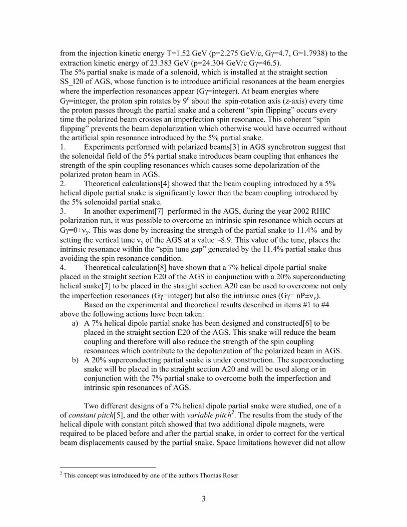
Figure 1: Cross section of a W_magnet. The cross section of the magnet occupies an area of 90 cm x 50 cm. The red colored areas are the conductor-coils of the magnet. The magnet has been excited at 1.5 [T] and the colored regions shown on the surface of the iron, correspond to the strength of the magnetic field (Bmod) at various regions of the iron of the magnet. The strength of the Bmod field that corresponds to each color is shown in the “scale” drawn at the bottom of the figure.

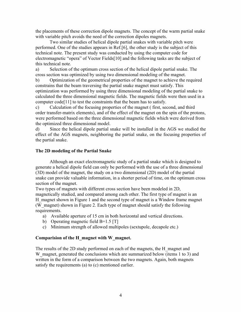
Figure 2: Cross section of an H_magnet. The magnet occupies an area of 100 cm x 80 cm. The red areas are the conductor coils of the magnet. The magnet has been excited at 1.5 [T] and the colored regions signify

6

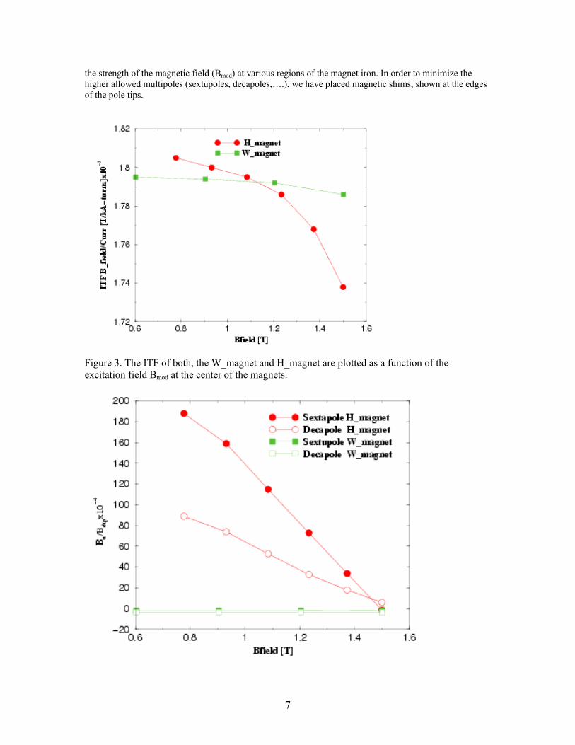
the strength of the magnetic field (Bmod) at various regions of the magnet iron. In order to minimize the higher allowed multipoles (sextupoles, decapoles,….), we have placed magnetic shims, shown at the edges of the pole tips.

Figure 3. The ITF of both, the W_magnet and H_magnet are plotted as a function of the excitation field Bmod at the center of the magnets.

7

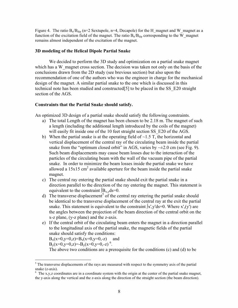
Figure 4. The ratio Bn/Bdip (n=2 Sextupole, n=4, Decapole) for the H_magnet and W_magnet as a function of the excitation field of the magnet. The ratio Bn/Bdip corresponding to the W_magnet remains almost independent of the excitation of the magnet.

3D modeling of the Helical Dipole Partial Snake

We decided to perform the 3D study and optimization on a partial snake magnet which has a W_magnet cross section. The decision was taken not only on the basis of the conclusions drawn from the 2D study (see brevious section) but also upon the recommendation of one of the authors who was the engineer in charge for the mechanical design of the magnet. A similar partial snake to the one which is discussed in this technical note has been studied and constructed[5] to be placed in the SS_E20 straight section of the AGS. Constraints that the Partial Snake should satisfy. An optimized 3D design of a partial snake should satisfy the following constraints.

a) The total Length of the magnet has been chosen to be 2.18 m. The magnet of such a length (including the additional length introduced by the coils of the magnet) will easily fit inside one of the 10 feet straight section SS_E20 of the AGS.

b) When the partial snake is at the operating field of ~1.5 T, the horizontal and vertical displacement of the central ray of the circulating beam inside the partial snake from the “optimum closed orbit” in AGS, varies by ~±2.0 cm (see Fig. 9). Such beam displacements may cause beam losses due to the interaction of the particles of the circulating beam with the wall of the vacuum pipe of the partial snake. In order to minimize the beam losses inside the partial snake we have allowed a 15x15 cm2 available aperture for the beam inside the partial snake magnet.

c) The central ray entering the partial snake should exit the partial snake in a direction parallel to the direction of the ray entering the magnet. This statement is equivalent to the constraint ∫Bx,yds=0.

d) The transverse displacement5 of the central ray entering the partial snake should be identical to the transverse displacement of the central ray at the exit the partial snake. This statement is equivalent to the constraint ∫x',y'ds=0. Where x',(y') are the angles between the projection of the beam direction of the central orbit on the x-z plane, (y-z plane) and the z-axis.

e) If the central orbit of the circulating beam enters the magnet in a direction parallel to the longitudinal axis of the partial snake, the magnetic fields of the partial snake should satisfy the conditions: Bx(x=0,y=0,z)=Bx(x=0,y=0,-z) and By(x=0,y=0,z)=-By(x=0,y=0,-z) 6. The above two conditions are a prerequisite for the conditions (c) and (d) to be

5 The transverse displacements of the rays are measured with respect to the symmetry axis of the partial snake (z-axis). 6 The x,y,z coordinates are in a coordinate system with the origin at the center of the partial snake magnet, the y-axis along the vertical and the z-axis along the direction of the straight section (the beam direction).

8

fulfilled. f) If the energy of the proton is such that the condition Gγ=integer, the partial snake

should rotate the proton spin by ~13o about the axis of the partial snake every time the proton traverses the partial snake. The required helical magnetic field for the 13o spin rotation is ~1.5 [T].

Available Geometrical Degrees of Freedom used in the design a Partial Snake The concept of the helical dipole partial snake with variable pitch provides enough degrees of freedom which can be adjusted in order to satisfy the constraints of the partial snake discussed in the previous section. The available degrees of freedom are:

a) The total length of the magnet is comprised of three sections. The first and the third sections of the iron of the partial snake are of equal lengths of L1 each, and the central section is of length L2. The length of each section is variable and is subject to the constraint 2L1+L2=L where L =2.18 m is the length of the magnet.

b) The helical pitch of each section of the partial snake is variable. The pitch of the first and third sections of the iron are of equal magnitude.

Setting up the 3D model.

This section is useful to the readers that are interested to reproduce the 3D model of the partial snake magnet using the computer code “opera” of Vector Fields[10].

Generating the Helical sections of the Magnet Iron. This section provides details on the construction of the three dimensional model

of the partial snake. The helical dipole magnet is comprised of three helical sections (see Fig. 8) which

are all made of magnetic iron. In order to generate the three helical sections of the partial snake, each helical section is segmented into smaller subsections, which are referred to in this technical note as “layers”. The number of layers in the first and the third helical sections is the same, and each section has 25 layers. The thickness of each of the layers of the first and third sections is L1/25. The second helical section is subdivided into 30 layers with the thickness being L2/30. The exit face of each layer, in the first and third sections, is rotated with respect to the entrance face of the layer by an angle R1/25, and by an angle R2/30 for the layers of the middle section. The variable R1 is the total rotation angle between the front and back surfaces of either the first or third section and the variable R2 is the corresponding angle of rotation between the front and back surface of the middle section.

9

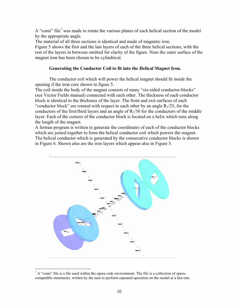
A “comi” file7 was made to rotate the various planes of each helical section of the model by the appropriate angle. The material of all three sections is identical and made of magnetic iron. Figure 5 shows the first and the last layers of each of the three helical sections, with the rest of the layers in between omitted for clarity of the figure. Note the outer surface of the magnet iron has been chosen to be cylindrical.

Generating the Conductor Coil to fit into the Helical Magnet Iron.

The conductor coil which will power the helical magnet should fit inside the

opening if the iron core shown in figure 5. The coil inside the body of the magnet consists of many “six-sided conductor-blocks” (see Vector Fields manual) connected with each other. The thickness of each conductor block is identical to the thickness of the layer. The front and exit surfaces of each “conductor block” are rotated with respect to each other by an angle R1/25, for the conductors of the first/third layers and an angle of R2/30 for the conductors of the middle layer. Each of the corners of the conductor block is located on a helix which runs along the length of the magnet. A fortran program is written to generate the coordinates of each of the conductor blocks which are joined together to form the helical conductor coil which powers the magnet. The helical conductor which is generated by the consecutive conductor blocks is shown in Figure 6. Shown also are the iron layers which appear also in Figure 5.

.

10

7 A “comi” file is a file used within the opera code environment. The file is a collection of opera-compatible statements, written by the user to perform repeated operation on the model at a fast rate.

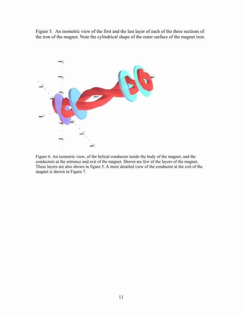
Figure 5. An isometric view of the first and the last layer of each of the three sections of the iron of the magnet. Note the cylindrical shape of the outer surface of the magnet iron.

Figure 6. An isometric view, of the helical conductor inside the body of the magnet, and the conductors at the entrance and exit of the magnet. Shown are few of the layers of the magnet. These layers are also shown in figure 5. A more detailed view of the conductor at the exit of the magnet is shown in Figure 7.

11

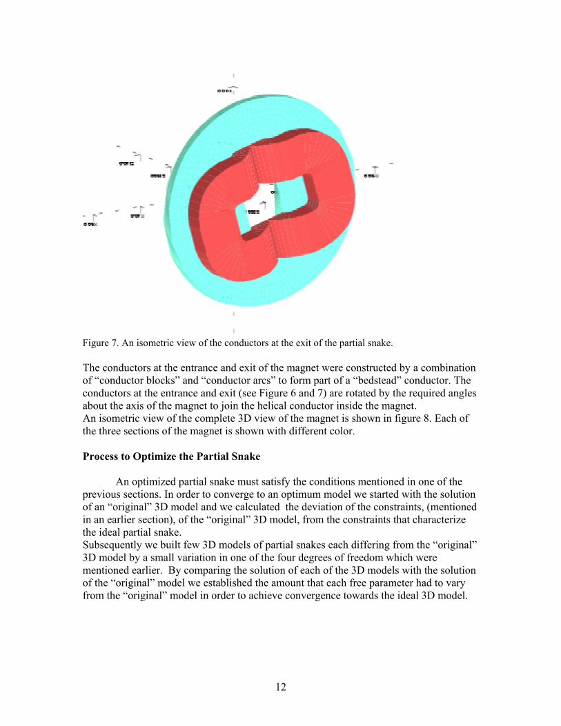
Figure 7. An isometric view of the conductors at the exit of the partial snake. The conductors at the entrance and exit of the magnet were constructed by a combination of “conductor blocks” and “conductor arcs” to form part of a “bedstead” conductor. The conductors at the entrance and exit (see Figure 6 and 7) are rotated by the required angles about the axis of the magnet to join the helical conductor inside the magnet. An isometric view of the complete 3D view of the magnet is shown in figure 8. Each of the three sections of the magnet is shown with different color. Process to Optimize the Partial Snake

An optimized partial snake must satisfy the conditions mentioned in one of the previous sections. In order to converge to an optimum model we started with the solution of an “original” 3D model and we calculated the deviation of the constraints, (mentioned in an earlier section), of the “original” 3D model, from the constraints that characterize the ideal partial snake. Subsequently we built few 3D models of partial snakes each differing from the “original” 3D model by a small variation in one of the four degrees of freedom which were mentioned earlier. By comparing the solution of each of the 3D models with the solution of the “original” model we established the amount that each free parameter had to vary from the “original” model in order to achieve convergence towards the ideal 3D model.

12

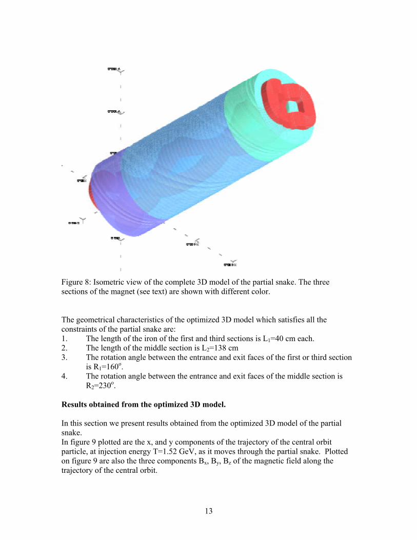
Figure 8: Isometric view of the complete 3D model of the partial snake. The three sections of the magnet (see text) are shown with different color. The geometrical characteristics of the optimized 3D model which satisfies all the constraints of the partial snake are: 1. The length of the iron of the first and third sections is L1=40 cm each. 2. The length of the middle section is L2=138 cm 3. The rotation angle between the entrance and exit faces of the first or third section

is R1=160o. 4. The rotation angle between the entrance and exit faces of the middle section is

R2=230o. Results obtained from the optimized 3D model. In this section we present results obtained from the optimized 3D model of the partial snake. In figure 9 plotted are the x, and y components of the trajectory of the central orbit particle, at injection energy T=1.52 GeV, as it moves through the partial snake. Plotted on figure 9 are also the three components Bx, By, Bz of the magnetic field along the trajectory of the central orbit.

13

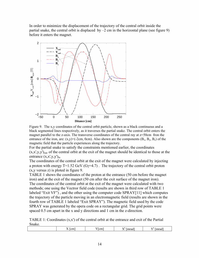
In order to minimize the displacement of the trajectory of the central orbit inside the partial snake, the central orbit is displaced by –2 cm in the horizontal plane (see figure 9) before it enters the magnet.

−50 0 50 100 150 200 250Ditance [cm]

−2

−1

0

1

2

Xco

d,Yco

d,,[

cm]

Bx,

y,z [

T]

Xcod

Ycod

Bx

By

Bz

Figure 9. The x,y coordinates of the central orbit particle, shown as a black continuous and a black segmented lines respectively, as it traverses the partial snake. The central orbit enters the magnet parallel to the z-axis. The transverse coordinates of the central ray at z=50cm fron the entrance of the iron, are: (x,y)=(-2cm, 0cm). Also shown are the components (Bx, By, Bz) of the magnetic field that the particle experiences along the trajectory. For the partial snake to satisfy the constraints mentioned earlier, the coordinates (x,x',y,y')out of the central orbit at the exit of the magnet should be identical to those at the entrance (x,x',y,y')in The coordinates of the central orbit at the exit of the magnet were calculated by injecting a proton with energy T=1.52 GeV (Gγ=4.7) . The trajectory of the central orbit proton (x,y versus z) is ploted in figure 9. TABLE 1 shows the coordinates of the proton at the entrance (50 cm before the magnet iron) and at the exit of the magnet (50 cm after the exit surface of the magnet iron). The coordinates of the central orbit at the exit of the magnet were calculated with two methods; one using the Vectror field code (results are shown in third row of TABLE 1 labeled “Exit VF”) , and the other using the computer code SPRAY[11] which computes the trajectory of the particle moving in an electromagnetic field (results are shown in the fourth row of TABLE 1 labeled “Exit SPRAY”). The magnetic field used by the code SPRAY was generated by the opera code on a rectangular grid. The grid points were spaced 0.5 cm apart in the x and y directions and 1 cm in the z-direction. TABLE 1: Coordinates (x,x') of the central orbit at the entrance and exit of the Partial Snake.

X [cm] Y[cm] X' [mrad] Y' [mrad]

14

entrance -2.000 0.000 0.000 0.000 Exit_VF -1.975 -0.150 -0.049 0.002

Exit_SPRAY -1.984 -0.148 -0.107 0.003 Looking at the results of TABLE 1 we conclude that the optimized partial snake does NOT fully satisfy all the constraints mentioned earlier. An additional computer iteration was required with new geometrical parameters (L1,L2,R1,R2) of the partial snake, to achieve the ideal solution. However we did not perform the additional iteration because the deviations of the computed values from the ideal ones are within the errors that the mechanical tolerances can generate. These errors can be corrected with the correction dipoles of the AGS Synchrotron.

An alternative but equivalent way to test how “close” the optimized partial snake magnet is to the ideal magnet, is to compute the integrals ∫Bx,yds and ∫x′,y′ds where Bx,y are the field components along the trajectory of the central orbit (see figure 9) and x′,(y′) are the angles between the projection of the momentum of the central orbit on the x-z plane,(y-z plane), and the z-axis. The coordinates x′,y′ of the central orbit along the trajectory were calculated by using the raytrace module of the computer code “opera” and are plotted as a function of distance z along the magnet, in figure 10. In Table 2 the following quantities are shown: a) Third row labeled “Ideal” shows the quantities xout-xin , yout-yin x′out-x′in , y′out-y′in and the equivalent quantities ∫x′ds, ∫y′ds, ∫Byds/(Bρ), ∫Bxds/(Bρ) which all have to be zero for an ideal Partial Snake. b) The fourth row labeled “DIFF_VF” shows the quantities xout-xin , yout-yin x′out-x′in , y′out-y′in (Difference of rows 3 and 2 of Table 1 ) as calculated using the opera computer code. c) The fifth row labeled “DIFF_SPRAY” shows the quantities xout-xin , yout-yin x′out-x′in , y′out-y′in (Difference of rows 4 and 2 of Table 1 ) as calculated using the computer code SPRAY. d) The sixth row labeled “INT_SPRAY” shows the quantities ∫x′ds, ∫y′ds, ∫Byds/(Bρ), ∫Bxds/(Bρ) as calculated using the computer code SPRAY. TABLE 2: The quantities xout-xin , yout-yin x′out-x′in , y′out-y′in and the equivalent ∫x′ds, ∫y′ds, ∫Byds/(Bρ), ∫Bxds/(Bρ) as calculated using various methods, (see text).

∫x′ds or xout-xin ∫y′ds or yout-yin ∫Byds/(Bρ) or x′out-x′in ∫Bxds/(Bρ) or y′out-y′in [cm] [cm] [mrad] [mrad]

Ideal 0 0 0 0 DIFF_VF 0.025 -0.150 -0.049 0.002

DIFF_SPAY 0.016 -0.148 -0.107 0.003

INT_SPRAY 0.025 -0.152 -0.138 0.020

15

−50 0 50 100 150 200 250Distance [cm]

−0.075

−0.050

−0.025

0.000

0.025

0.050

0.075

x’,y

’ [m

rad]

x’y’

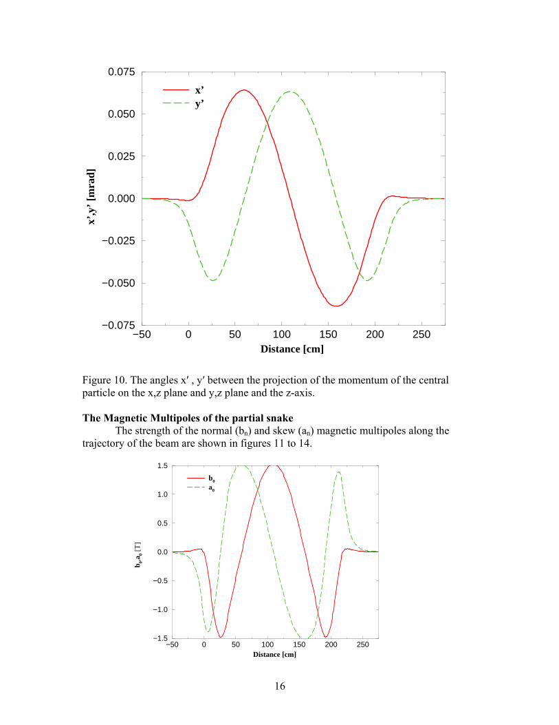
Figure 10. The angles x′ , y′ between the projection of the momentum of the central particle on the x,z plane and y,z plane and the z-axis. The Magnetic Multipoles of the partial snake

The strength of the normal (bn) and skew (an) magnetic multipoles along the trajectory of the beam are shown in figures 11 to 14.

−50 0 50 100 150 200 250Distance [cm]

−1.5

−1.0

−0.5

0.0

0.5

1.0

1.5

b 0,a0 [

T]

b0

a0

16

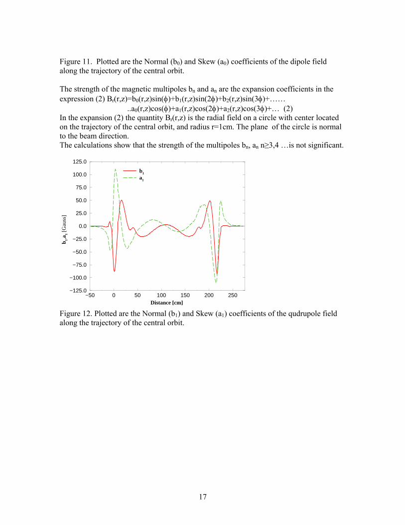
Figure 11. Plotted are the Normal (b0) and Skew (a0) coefficients of the dipole field along the trajectory of the central orbit. The strength of the magnetic multipoles bn and an are the expansion coefficients in the expression (2) Br(r,z)=b0(r,z)sin(φ)+b1(r,z)sin(2φ)+b2(r,z)sin(3φ)+…… ..a0(r,z)cos(φ)+a1(r,z)cos(2φ)+a2(r,z)cos(3φ)+… (2) In the expansion (2) the quantity Br(r,z) is the radial field on a circle with center located on the trajectory of the central orbit, and radius r=1cm. The plane of the circle is normal to the beam direction. The calculations show that the strength of the multipoles bn, an n≥3,4 …is not significant.

−50 0 50 100 150 200 250Distance [cm]

−125.0

−100.0

−75.0

−50.0

−25.0

0.0

25.0

50.0

75.0

100.0

125.0

b 1,a1 [

Gau

ss]

b1

a1

Figure 12. Plotted are the Normal (b1) and Skew (a1) coefficients of the qudrupole field along the trajectory of the central orbit.

17

−50 0 50 100 150 200 250Distance [cm]

−25.0

−20.0

−15.0

−10.0

−5.0

0.0

5.0

10.0

15.0

20.0

25.0

b 2,a2 [

Gau

ss]

b2

a2

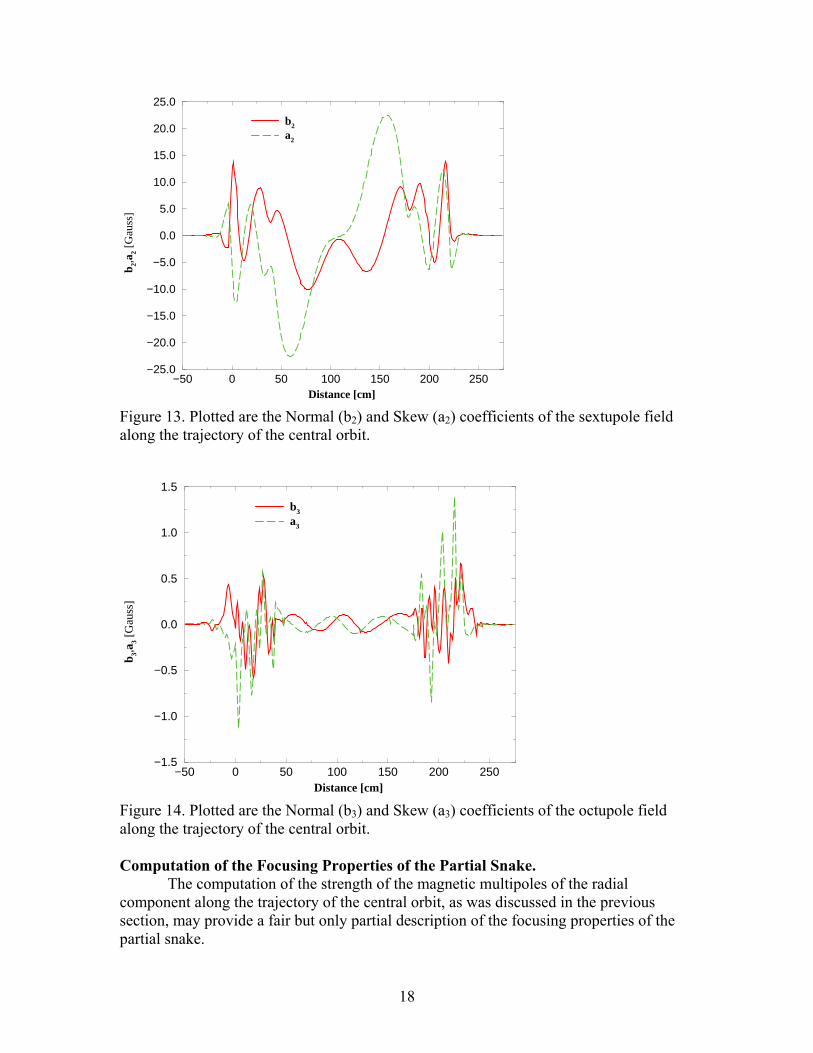
Figure 13. Plotted are the Normal (b2) and Skew (a2) coefficients of the sextupole field along the trajectory of the central orbit.

−50 0 50 100 150 200 250Distance [cm]

−1.5

−1.0

−0.5

0.0

0.5

1.0

1.5

b 3,a3 [

Gau

ss]

b3

a3

Figure 14. Plotted are the Normal (b3) and Skew (a3) coefficients of the octupole field along the trajectory of the central orbit. Computation of the Focusing Properties of the Partial Snake.

The computation of the strength of the magnetic multipoles of the radial component along the trajectory of the central orbit, as was discussed in the previous section, may provide a fair but only partial description of the focusing properties of the partial snake.

18

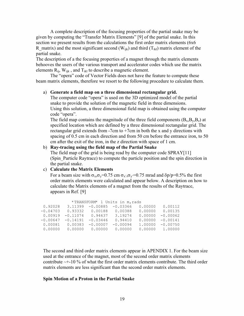
A complete description of the focusing properties of the partial snake may be given by computing the “Transfer Matrix Elements” [9] of the partial snake. In this section we present results from the calculations the first order matrix elements (6x6 R_matrix) and the most significant second (Wijk) and third (Tikl) matrix element of the partial snake. The description of a the focusing properties of a magnet through the matrix elements behooves the users of the various transport and accelerator codes which use the matrix elements Rij, Wijk , and Tikl to describe a magnetic element.

The “opera” code of Vector Fields does not have the feature to compute these beam matrix elements, therefore we resort to the following procedure to calculate them.

a) Generate a field map on a three dimensional rectangular grid.

The computer code “opera” is used on the 3D optimized model of the partial snake to provide the solution of the magnetic field in three dimensions. Using this solution, a three dimensional field map is obtained using the computer code “opera”. The field map contains the magnitude of the three field components (Bx,By,Bz) at specified location which are defined by a three dimensional rectangular grid. The rectangular grid extends from -7cm to +7cm in both the x and y directions with spacing of 0.5 cm in each direction and from 50 cm before the entrance iron, to 50 cm after the exit of the iron, in the z direction with space of 1 cm.

b) Ray-tracing using the field map of the Partial Snake The field map of the grid is being read by the computer code SPRAY[11] (Spin_Particle Raytrace) to compute the particle position and the spin direction in the partial snake.

c) Calculate the Matrix Elements For a beam size with σx,σy=0.75 cm σx’,σy’=0.75 mrad and δp/p=0.5% the first order matrix elements were calculated and appear below. A description on how to calculate the Matrix elements of a magnet from the results of the Raytrace, appears in Ref. [9]

*TRANSFORM* 1 Units in m,rads 0.92028 3.11399 -0.00885 -0.03366 0.00000 0.00112 -0.04703 0.93332 0.00188 0.00388 0.00000 0.00135 0.00919 -0.11074 0.94637 3.19274 0.00000 -0.00062 -0.00647 -0.14191 -0.03446 0.94410 0.00000 -0.00141 0.00081 0.00383 -0.00007 -0.00094 1.00000 -0.00750 0.00000 0.00000 0.00000 0.00000 0.00000 1.00000

The second and third order matrix elements appear in APENDIX 1. For the beam size used at the entrance of the magnet, most of the second order matrix elements contribute ~+-10 % of what the first order matrix elements contribute. The third order matrix elements are less significant than the second order matrix elements. Spin Motion of a Proton in the Partial Snake

19

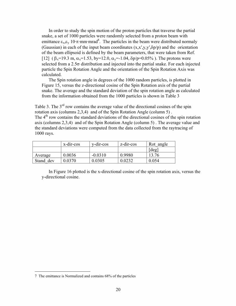
In order to study the spin motion of the proton particles that traverse the partial snake, a set of 1000 particles were randomly selected from a proton beam with emittance εx,εy 10·π·mm·mrad8. The particles in the beam were distributed normaly (Gaussian) in each of the input beam coordinates (x,x′,y,y′,δp/p) and the orientation of the beam ellipsoid is defined by the beam parameters, that were taken from Ref. [12] ( βx=19.3 m, αx=1.53, by=12.0, αy=-1.04, δp/p=0.05% ). The protons were selected from a 2.5σ distribution and injected into the partial snake. For each injected particle the Spin Rotation Angle and the orientation of the Spin Rotation Axis was calculated.

The Spin rotation angle in degrees of the 1000 random particles, is plotted in Figure 15, versus the z-directional cosine of the Spin Rotation axis of the partial snake. The average and the standard deviation of the spin rotation angle as calculated from the information obtained from the 1000 particles is shown in Table 3

Table 3. The 3rd row contains the average value of the directional cosines of the spin rotation axis (columns 2,3,4) and of the Spin Rotation Angle (column 5) . The 4th row contains the standard deviations of the directional cosines of the spin rotation axis (columns 2,3,4) and of the Spin Rotation Angle (column 5) . The average value and the standard deviations were computed from the data collected from the raytracing of 1000 rays. x-dir-cos y-dir-cos z-dir-cos Rot_angle [deg] Average 0.0036 -0.0310 0.9980 13.76 Stand_dev 0.0370 0.0305 0.0232 0.054

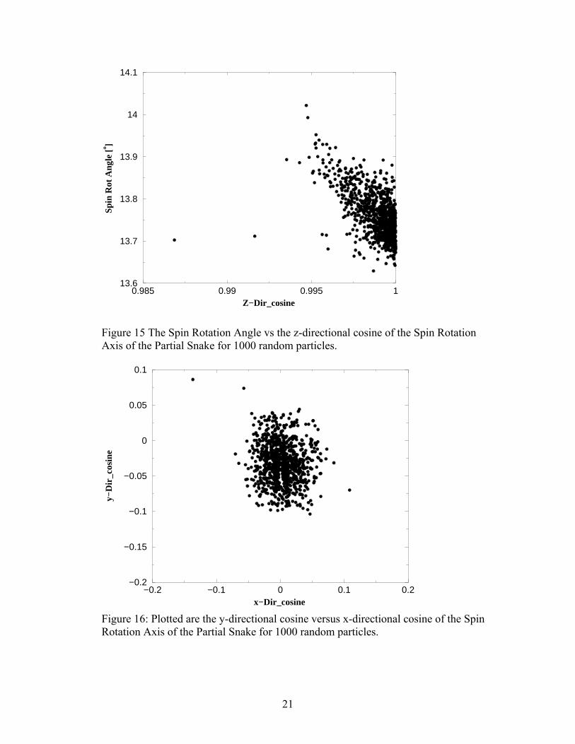
In Figure 16 plotted is the x-directional cosine of the spin rotation axis, versus the

y-directional cosine.

7 The emittance is Normalized and contains 68% of the particles

20

0.985 0.99 0.995 1Z−Dir_cosine

13.6

13.7

13.8

13.9

14

14.1

Spi

n R

ot A

ngle

[o ]

Figure 15 The Spin Rotation Angle vs the z-directional cosine of the Spin Rotation Axis of the Partial Snake for 1000 random particles.

−0.2 −0.1 0 0.1 0.2x−Dir_cosine

−0.2

−0.15

−0.1

−0.05

0

0.05

0.1

y−

Dir_

cosi

ne

Figure 16: Plotted are the y-directional cosine versus x-directional cosine of the Spin Rotation Axis of the Partial Snake for 1000 random particles.

21

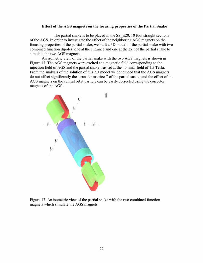
Effect of the AGS magnets on the focusing properties of the Partial Snake The partial snake is to be placed in the SS_E20, 10 foot straight sections

of the AGS. In order to investigate the effect of the neighboring AGS magnets on the focusing properties of the partial snake, we built a 3D model of the partial snake with two combined function dipoles, one at the entrance and one at the exit of the partial snake to simulate the two AGS magnets.

An isometric view of the partial snake with the two AGS magnets is shown in Figure 17. The AGS magnets were excited at a magnetic field corresponding to the injection field of AGS and the partial snake was set at the nominal field of 1.5 Tesla. From the analysis of the solution of this 3D model we concluded that the AGS magnets do not affect significantly the “transfer matrices” of the partial snake, and the effect of the AGS magnets on the central orbit particle can be easily corrected using the corrector magnets of the AGS.

Figure 17. An isometric view of the partial snake with the two combined function magnets which simulate the AGS magnets.

22

REFERANCES [1] T. Roser, AIP Conf. Proc. 187 (1988) 1221. [2] H.Huang, et. al. Phys. Rev. Lett. 73 (1994) 2982 [3] M.Bai, et. al. Workshop on Increasing the AGS Polarization, University of Michigan, Ann Arbor, Michigan, Nov. 6-9 2002 [4[ N. Tsoupas BNL, Private comunication. [5] Design Study of Helical Partial Snake Magnet for AGS M. Okamura, T. Tominaka and T. Katayama RIKEN,Japan N. Tsoupas, BNL, USA EPAC 2002, Paris France, June 2-7, 2002 [6] Design Study of a Normal Conducting Helical Snake for AGS Junpei Takano, et. al. [7] 20% Partial Siberian Snake in the AGS H. Huang et. al. BNL Workshop on Increasing the AGS Polarization, University of Michigan, Ann Arbor, Michigan, Nov. 6-9 2002 BNL-71492-2003-CP [8] Thomas Roser, BNL, Private communication. [9] Feasibility study of a Method to Measure the focusing properties (R_Matrix) of a magnet N. Tsoupas, et. al. Technical Note CAD/AD #135 Feb 2004 [10] Vector Fields Limited, Oxford, UK [11] A computer code for Spin and Particle Raytrace (SPRAY) in an Electromagnetic Field. N. Tsoupas BNL Private Communication. [12] Closed Orbit Calculations at AGS and Extraction-Beam-Parameters at H13 N.Tsoupas, H.W. Foelsche, J. Claus, R. Thern AD/RHIC/RD-75

23

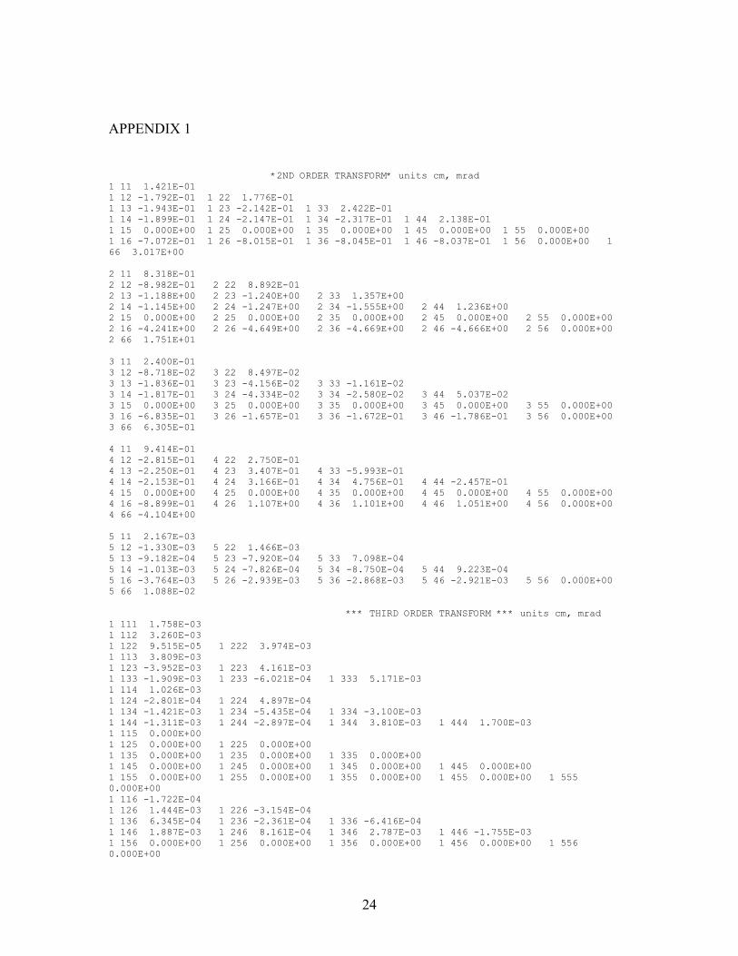
APPENDIX 1 *2ND ORDER TRANSFORM* units cm, mrad 1 11 1.421E-01 1 12 -1.792E-01 1 22 1.776E-01 1 13 -1.943E-01 1 23 -2.142E-01 1 33 2.422E-01 1 14 -1.899E-01 1 24 -2.147E-01 1 34 -2.317E-01 1 44 2.138E-01 1 15 0.000E+00 1 25 0.000E+00 1 35 0.000E+00 1 45 0.000E+00 1 55 0.000E+00 1 16 -7.072E-01 1 26 -8.015E-01 1 36 -8.045E-01 1 46 -8.037E-01 1 56 0.000E+00 1 66 3.017E+00 2 11 8.318E-01 2 12 -8.982E-01 2 22 8.892E-01 2 13 -1.188E+00 2 23 -1.240E+00 2 33 1.357E+00 2 14 -1.145E+00 2 24 -1.247E+00 2 34 -1.555E+00 2 44 1.236E+00 2 15 0.000E+00 2 25 0.000E+00 2 35 0.000E+00 2 45 0.000E+00 2 55 0.000E+00 2 16 -4.241E+00 2 26 -4.649E+00 2 36 -4.669E+00 2 46 -4.666E+00 2 56 0.000E+00 2 66 1.751E+01 3 11 2.400E-01 3 12 -8.718E-02 3 22 8.497E-02 3 13 -1.836E-01 3 23 -4.156E-02 3 33 -1.161E-02 3 14 -1.817E-01 3 24 -4.334E-02 3 34 -2.580E-02 3 44 5.037E-02 3 15 0.000E+00 3 25 0.000E+00 3 35 0.000E+00 3 45 0.000E+00 3 55 0.000E+00 3 16 -6.835E-01 3 26 -1.657E-01 3 36 -1.672E-01 3 46 -1.786E-01 3 56 0.000E+00 3 66 6.305E-01 4 11 9.414E-01 4 12 -2.815E-01 4 22 2.750E-01 4 13 -2.250E-01 4 23 3.407E-01 4 33 -5.993E-01 4 14 -2.153E-01 4 24 3.166E-01 4 34 4.756E-01 4 44 -2.457E-01 4 15 0.000E+00 4 25 0.000E+00 4 35 0.000E+00 4 45 0.000E+00 4 55 0.000E+00 4 16 -8.899E-01 4 26 1.107E+00 4 36 1.101E+00 4 46 1.051E+00 4 56 0.000E+00 4 66 -4.104E+00 5 11 2.167E-03 5 12 -1.330E-03 5 22 1.466E-03 5 13 -9.182E-04 5 23 -7.920E-04 5 33 7.098E-04 5 14 -1.013E-03 5 24 -7.826E-04 5 34 -8.750E-04 5 44 9.223E-04 5 16 -3.764E-03 5 26 -2.939E-03 5 36 -2.868E-03 5 46 -2.921E-03 5 56 0.000E+00 5 66 1.088E-02 *** THIRD ORDER TRANSFORM *** units cm, mrad 1 111 1.758E-03 1 112 3.260E-03 1 122 9.515E-05 1 222 3.974E-03 1 113 3.809E-03 1 123 -3.952E-03 1 223 4.161E-03 1 133 -1.909E-03 1 233 -6.021E-04 1 333 5.171E-03 1 114 1.026E-03 1 124 -2.801E-04 1 224 4.897E-04 1 134 -1.421E-03 1 234 -5.435E-04 1 334 -3.100E-03 1 144 -1.311E-03 1 244 -2.897E-04 1 344 3.810E-03 1 444 1.700E-03 1 115 0.000E+00 1 125 0.000E+00 1 225 0.000E+00 1 135 0.000E+00 1 235 0.000E+00 1 335 0.000E+00 1 145 0.000E+00 1 245 0.000E+00 1 345 0.000E+00 1 445 0.000E+00 1 155 0.000E+00 1 255 0.000E+00 1 355 0.000E+00 1 455 0.000E+00 1 555 0.000E+00 1 116 -1.722E-04 1 126 1.444E-03 1 226 -3.154E-04 1 136 6.345E-04 1 236 -2.361E-04 1 336 -6.416E-04 1 146 1.887E-03 1 246 8.161E-04 1 346 2.787E-03 1 446 -1.755E-03 1 156 0.000E+00 1 256 0.000E+00 1 356 0.000E+00 1 456 0.000E+00 1 556 0.000E+00

24

1 166 -1.564E-03 1 266 1.168E-03 1 366 1.607E-03 1 466 -5.082E-03 1 566 0.000E+00 1 666 -7.711E-03 2 111 7.332E-03 2 112 4.025E-03 2 122 3.877E-03 2 222 -2.172E-02 2 113 5.911E-02 2 123 -5.842E-02 2 223 5.446E-02 2 133 -6.047E-03 2 233 -2.876E-04 2 333 -4.103E-02 2 114 -6.049E-04 2 124 -3.423E-03 2 224 -5.150E-05 2 134 -1.443E-02 2 234 -9.060E-03 2 334 -4.035E-02 2 144 -2.911E-03 2 244 3.204E-03 2 344 4.947E-02 2 444 -1.523E-02 2 115 0.000E+00 2 125 0.000E+00 2 225 0.000E+00 2 135 0.000E+00 2 235 0.000E+00 2 335 0.000E+00 2 145 0.000E+00 2 245 0.000E+00 2 345 0.000E+00 2 445 0.000E+00 2 155 0.000E+00 2 255 0.000E+00 2 355 0.000E+00 2 455 0.000E+00 2 555 0.000E+00 2 116 -2.901E-03 2 126 1.270E-02 2 226 -4.495E-03 2 136 6.770E-03 2 236 6.202E-04 2 336 -6.438E-03 2 146 1.987E-02 2 246 8.968E-03 2 346 1.790E-02 2 446 -1.064E-02 2 156 0.000E+00 2 256 0.000E+00 2 356 0.000E+00 2 456 0.000E+00 2 556 0.000E+00 2 166 -1.324E-02 2 266 6.653E-03 2 366 7.928E-03 2 466 -3.228E-02 2 566 0.000E+00 2 666 -1.291E-01 3 111 -1.930E-02 3 112 7.691E-03 3 122 7.923E-04 3 222 1.728E-02 3 113 -4.866E-03 3 123 8.489E-04 3 223 -4.595E-03 3 133 2.064E-03 3 233 3.916E-03 3 333 -1.404E-02 3 114 -1.342E-03 3 124 2.616E-04 3 224 -1.873E-04 3 134 8.775E-04 3 234 -3.293E-04 3 334 9.989E-03 3 144 -1.567E-04 3 244 2.585E-04 3 344 2.548E-03 3 444 -9.555E-03 3 115 0.000E+00 3 125 0.000E+00 3 225 0.000E+00 3 135 0.000E+00 3 235 0.000E+00 3 335 0.000E+00 3 145 0.000E+00 3 245 0.000E+00 3 345 0.000E+00 3 445 0.000E+00 3 155 0.000E+00 3 255 0.000E+00 3 355 0.000E+00 3 455 0.000E+00 3 555 0.000E+00 3 116 1.398E-04 3 126 -9.197E-04 3 226 2.590E-04 3 136 -7.718E-04 3 236 -1.631E-04 3 336 1.314E-03 3 146 -2.710E-04 3 246 -7.431E-04 3 346 -1.382E-03 3 446 1.651E-03 3 156 0.000E+00 3 256 0.000E+00 3 356 0.000E+00 3 456 0.000E+00 3 556 0.000E+00 3 166 3.114E-03 3 266 -5.016E-04 3 366 -1.930E-03 3 466 1.169E-03 3 566 0.000E+00 3 666 1.179E-02 4 111 -2.238E-02 4 112 9.223E-02 4 122 9.043E-03 4 222 1.979E-01 4 113 -2.954E-02 4 123 6.118E-03 4 223 -2.895E-02 4 133 -1.148E-03 4 233 2.533E-02 4 333 -6.114E-02 4 114 -1.623E-02 4 124 7.036E-03 4 224 -5.580E-03 4 134 1.616E-02 4 234 -3.754E-04 4 334 6.114E-02 4 144 -6.583E-03 4 244 2.930E-03 4 344 4.687E-02 4 444 -4.279E-02 4 115 0.000E+00 4 125 0.000E+00 4 225 0.000E+00 4 135 0.000E+00 4 235 0.000E+00 4 335 0.000E+00 4 145 0.000E+00 4 245 0.000E+00 4 345 0.000E+00 4 445 0.000E+00 4 155 0.000E+00 4 255 0.000E+00 4 355 0.000E+00 4 455 0.000E+00 4 555 0.000E+00 4 116 3.054E-03 4 126 -7.027E-03 4 226 4.822E-03

25

26

4 136 -7.737E-03 4 236 -3.456E-03 4 336 9.925E-03 4 146 -2.447E-03 4 246 -7.550E-03 4 346 -5.789E-03 4 446 8.981E-03 4 156 0.000E+00 4 256 0.000E+00 4 356 0.000E+00 4 456 0.000E+00 4 556 0.000E+00 4 166 1.832E-02 4 266 -1.662E-03 4 366 -1.037E-02 4 466 3.783E-03 4 566 0.000E+00 4 666 2.031E-01 5 111 -6.345E-05 5 112 -1.711E-04 5 122 -3.396E-06 5 222 -2.893E-04 5 113 -5.739E-06 5 133 1.689E-05 5 233 -6.794E-06 5 333 -4.116E-06 5 114 2.005E-05 5 124 -6.581E-06 5 224 3.549E-06 5 134 -2.126E-05 5 234 1.750E-06 5 334 1.016E-04 5 115 0.000E+00 5 125 0.000E+00 5 225 0.000E+00 5 135 0.000E+00 5 235 0.000E+00 5 335 0.000E+00 5 145 0.000E+00 5 245 0.000E+00 5 345 0.000E+00 5 445 0.000E+00 5 155 0.000E+00 5 255 0.000E+00 5 355 0.000E+00 5 455 0.000E+00 5 555 0.000E+00 5 116 -1.896E-05 5 126 1.983E-06 5 226 -1.360E-05 5 136 -1.015E-05 5 236 2.215E-05 5 336 6.224E-06 5 146 -1.451E-05 5 246 9.475E-06 5 346 -2.449E-05 5 446 1.163E-05 5 156 0.000E+00 5 256 0.000E+00 5 356 0.000E+00 5 456 0.000E+00 5 556 0.000E+00 5 166 5.804E-05 5 266 -3.310E-05 5 366 -2.074E-05 5 466 1.048E-05 5 566 0.000E+00 5 666 -6.106E-04