CALCULATION OF MINIMUM CRITICAL REYNOLDS NUMBER …etna.mcs.kent.edu/vol.30.2008/pp168-186.dir/pp168-186.pdf · Osborne Reynolds found two critical Reynolds num-bers ( ) in pipe o

Electronic Transactions on Numerical Analysis.Volume 30, pp. 168-186, 2008.Copyright 2008, Kent State University.ISSN 1068-9613.

ETNAKent State University

http://etna.math.kent.edu

CALCULATION OF MINIMUM CRITICAL REYNOLDS NUMBER FORLAMINAR-TURBULENT TRANSITION IN PIPE FLOWS

�HIDESADA KANDA

�Abstract. This article describes the calculation of the minimum critical Reynolds number for laminar-turbulent

transition in pipe flows. From the conclusions of our previous experimental study, it is clear that a transition occursnear the pipe inlet and the critical Reynolds number �� takes the minimum value of about 2000 in the case of astraight pipe. Moreover, in our previous calculations of laminar entrance pipe flow, it was found that near the pipeinlet a large pressure gradient in the radial direction exists, which decreases as the Reynolds number Re increases.Thus, we have built a new transition macromodel to determine �� using the effect of the radial pressure gradient.The calculated results were �� = 3750 when the number of radial grid points �� = 51 and 2200 when�� = 101.

Key words. hydrodynamic stability, grid refinement, thermodynamics

AMS subject classifications. 76E05, 65M50, 80A05

1. Introduction and summary. Osborne Reynolds found two critical Reynolds num-bers ( �� ) in pipe flows: �� of 12,830 from laminar to turbulent flow and �� of 2030 fromturbulent to laminar flow [16]. Ever since the pioneering experimental work of Reynolds(1883), the issue of how and why the fluid flow along a circular pipe changes from beinglaminar to turbulent as the flow rate increases has intrigued physicists, mathematicians, andengineers alike [11].

The objectives of this investigation are to derive a macromodel of laminar-turbulent tran-sition for Hagen-Poiseuille flow or pipe flow and to calculate the minimum value of the criti-cal Reynolds number ��! �"$# , which is in the neighborhood of 2000.

To date, attempts to theoretically obtain values of �� have been undertaken using stabilitytheory with the Orr-Sommerfeld equation and disturbances. However, �%�&��! �"$# of approxi-mately 2000 has not yet been calculated. For flow in the entrance region, Tatsumi obtained�� = 19,400 [21], and Huang and Chen obtained �� = 39,800 and 39,560 with axisymmetricand non-axisymmetric disturbances, respectively [5, 6]. In the fully developed region, theflow is stable with respect to both axisymmetric and non-axisymmetric disturbances [2]. Inthis study, we do not further consider such stability theory.

The line of thought on calculating �� for laminar-turbulent transition is formulated onthe basis of our experiments [10] and calculated results [8, 9].

(1) The Reynolds number (Re) primarily and generally affects � � , since transition occursas Re increases. Therefore, we must further study what factor, besides Re, mainly affects �'� .

(2) The laminar-turbulent transition occurs near the pipe inlet in the entrance region. It isimportant to note that the flow may become turbulent long before it becomes fully developed[4, 20].

(3) We must numerically find a new unknown variable which varies near the inlet. It isthe normal wall strength (NWS); see Subsection 3.1.

(4) We must numerically evaluate the effects of NWS on � � in this study.First, from the viewpoint of our experiments, let us consider the problem in more detail.(5) � � is apparently determined by the entrance shape or the contraction ratio(*)

(= + )-, + ) of the bellmouth diameter + ) to pipe diameter + . In most previous experi-.Received January 10, 2008. Accepted for publication March 19, 2008. Published online on July 23, 2008.

Recommended by F. Stenger.�Computer Science and Engineering, University of Aizu, Aizu-Wakamatsu, Fukushima 965-8580, Japan

([email protected]).

168



CALCULATION OF MINIMUM CRITICAL REYNOLDS NUMBER 169

Initial uniformvelocity profile (Uo)

Fully developedparabolic profile

xCenterline

0

r

Pipe wall

R D

Pipe wall

Dimensionless entrance length (Le = x’/(D Re))

Entrance length (x’)

FIG. 1.1. Velocity development in entrance region of a straight circular pipe.

ments, pipes were fitted with trumpet mouthpieces or bellmouths at the inlet, so that watermight enter without disturbances. ��/�0�1 2"$# of approximately 2000 is obtained in the caseof a straight circular pipe. The sharp edge of the straight pipe is not a singular point in thetransition, since �� is a smooth function of

( )at 3 2000.

(6) The transition occurs near the pipe inlet. For example, in the case of a straight pipe,the transition occurs approximately 6–13 diameters downstream at Re 3 2000. Consider a di-mensionless axial coordinate ( 4 ); let 576 be the actual axial coordinate, then 498:576 , �;+ Re # .For the above example, the transition occurs at the pipe inlet of 4=<?>�@ ,BABCDCEC 8 CGF CECDHDI .

(7) For Reynolds’ color-band experiments, �� varies when( )

= 1–2.3, particularly when(*)= 1–1.4. If the radial distance of

(J)= 1.4 is transformed to the axial distance to check the

order of length, then for Re 3 2000, 4K< 1.4/2000 = 0.0007.Second, let us consider the viewpoint of previous experimental and numerical results. In

the entrance region, the velocity profile changes from a uniform distribution at the pipe inletto a parabolic one at the entrance length, as shown in Fig. 1.1. Generally, thus far, three majorvariables have been studied [3]: (i) the velocity distribution in all sections, (ii) the entrancelength LNM , which is defined as the distance from the inlet to the point where the centerlinevelocity reaches 99 O of the fully developed value, and (iii) the pressure drop P'Q . The regionfrom the inlet to L M is called the entrance region and the downstream region from L M is calledthe fully developed region.L M [1] is expressed asLSRT8 5 6+ Re

8 CUF HDCRe � CGF C @ I Re VW>X# V CGF CDIEHGF

(1.1)

From (1.1), LYR = 0.0562 at Re = 300, and LYR takes a constant value of 0.056 at Re Z 500.The total pressure drop P'Q��4[# from the pipe inlet is expressed as the sum of the pressuredrop 64 4 that would occur if the flow were fully developed, plus the excess pressure drop\ ��4[# to account for the developing region.P'Q��4[#]89Q�� C #]^_Q��04[#[8 ^1Q��04`#a8 HEb 4cV \ �04`#\ ��4[# is assumed to be

\ ��de# in (1.2) for the fully developed region [1]. From (1.2),\ ��de#

is 1.276 at Re = 500 and 1.219 at Re = 2000.\ ��de# is approximately the same at Re Z 500.\ �2df#g8h> FiABC V @Ej

Re(1.2)



170 H. KANDA

(8) We discuss properties (a) and (b) of two parameters, which will enable us to determineaccurate values of �� : parameter (a) is a constant regardless of Re for Re Z 500 whileparameter (b) varies inversely as Re increases. The intersection of the lines of the parametersshould indicate a critical value; see Fig. 4.3.

(9) It is clear from (1.1) that the velocity distribution and L M in the 4 coordinate areapproximately the same at Re Z 500. Thus, parameter (a) of a constant magnitude is set to bethe increase in kinetic energy KE on the basis of the velocity development from a uniform toa parabolic profile; see Subsection 3.3. Concerning moving fluid particles, the physical unitof KE is power, i.e., energy per second.

(10) We found numerically that at Re 3k� � , a large pressure gradient exists in the normaldirection near the inlet and disappears as Re increases. This normal pressure gradient iscaused by NWS.

(11) We must evaluate the relationship between �� and the normal pressure gradient orNWS. The first law of thermodynamics (conservation of energy) states that the increase inthe energy of a material region is the result of work and heat transfers to the region [12]. Ifthere is no heat transfer, then some work is done on the fluid particles for KE. The physicalunits of energy and work are the same. Thus, parameter (b) is set to be the power RW doneby NWS.

Therefore, the main research subject is to numerically investigate the relationship amongKE, RW, and � � .

2. Calculation of radial pressure gradient.

2.1. Governing equations. First, we consider dimensionless variables. All lengths andvelocities are normalized by the pipe diameter + and the mean velocity lSm , respectively. Thepressure is normalized by �n> ,BA #poGl �m . Re is based on lqm and + . Note that the dimensionlessaxial coordinate 5 (= 5r6 , + ) is used for calculation and 4e�28W5r6 , ��+ Re #s# is used in our figuresand tables, where 5 6 is the actual axial coordinate.

We consider unsteady flow of an incompressible Newtonian fluid with a constant viscos-ity and density, and we disregard gravity and external forces. We introduce the streamfunctionand vorticity formulas in the two-dimensional cylindrical coordinates for the governing equa-tions in order to avoid the explicit appearance of the pressure term. Accordingly, the velocityfields are determined without any assumptions concerning the pressure. Subsequently, thepressure distribution is calculated using the values of the velocity fields.

The dimensionless transport equation for the vorticity is expressed astvutrw ^ >x tryt 5 tvut x V >x tryt x tvut 5 V ux � tryt 5 8 >Re

z tt xe{ >x t � x u #t x}| V t � ut 5 �*~ F(2.1)

The Poisson equation foru

is derived from the definition ofu

, i.e.,^ u 8�� y 8 tt x � >x tryt x #1V t �t 5 � � y x # F(2.2)

The axial velocity � and radial velocity � are defined as the derivatives of the streamfunction,i.e., �_8 >x tryt x�� 8 ^ >x tryt 5 F(2.3)

Only the angular ( � ) component of a two-dimensional flow fieldu

is non-negligible; thus, weshall replace

u��with

u, u 8 u�� 8�� ]�� 8 t �t 5 ^ t �t x F(2.4)




1

2

J0

Pipe wall

Pipe inlet

Flow

Pipe outlet

J1

J2

R

i i+11 I0

j

r

r

r

VrR -

∆ x

∆ x ∆ x

Centerline

FIG. 2.1. Grid system in a circular straight pipe.

The pressure can be calculated using the steady-state form of the Navier-Stokes (N-S)equations. The pressure distribution for the 5 derivative ist Qt 5 8 ^ A�� t �t 5 V�� t �t x�� V A

Re� t � �t 5 � V >x t �t x V t � �t x � � �(2.5)

and that for the x derivative ist Qt x 8 ^ A�� t �t 5 V�� t �t x � V ARe

� t � �t 5 � V >x t �t x ^ �x � V t � �t x � � F(2.6)

Since � and � are known at every point, from (2.3), a smooth pressure distribution that satis-fies both (2.5) and (2.6) is calculated using Poisson’s equation (2.7) [15],� � Q�8 t � Qt 5 � V t � Qt x � V >x t Qt x 8 ^ A�� t �t x � � V A t �t x t �t 5 V � t �t 5 � � V � �x �'� F(2.7)

In this study, initial values are obtained using (2.5), and then (2.7) is used to obtain bettersolutions.

2.2. Numerical method for vorticity transport equation. The rectangular grid systemused here is schematically illustrated in Fig. 2.1, where � C and � C are the maximum numbersfor axial and radial grid points, respectively, and �U>'8�� C ^W> � � A 8�� C ^ A � ��>%8_� C ^W> �and � A 8�� C ^ A .

To obtain precise results in this study, we used a refined axial grid of P!4�8 CGF CECDCEC > .For calculations, the dimensionless axial grid P!5��28�P!4:� Re) is used. The grid spaceP!5 6 �28�P!4��+�� Re) in actual length is considered. For a pipe of + = 2.6 cm andRe = 2000, the dimensionless grid space P!4 = 0.00001 corresponds to P!5 6 = 0.052 cmin actual length: P!5 6 = 0.00001 � 2.6 � 2000 = 0.052; for Re = 10,000, P!4 = 0.00001corresponds to P!5 6 = 0.26 cm in actual length. Two grid systems are used: (i) � C = 1001,� C = 51, and P!4 = 0.00001, and (ii) � C = 101. The maximum 4 is 0.01.

For unsteady problems, generally, an explicit method is faster than an implicit methodin CPU time, but lacks calculation stability. The finite difference equation for (2.1) was firstsolved by the Gauss-Seidel explicit iterative method [7, 8, 9], where calculation stability wasachieved by adding steps 4–5 in Fig. A.1; see Appendix. This explicit scheme, however,required long CPU times to maintain computational stability. Next, it was improved by the



172 H. KANDA

Start

1) Set initial and boundary conditions

2) CalculateuS�B� � from �uY�B� � and

yN�, Eq. (2.8), implicit

Check ¡r�u �B� � � � - �uY�B� � ¡E¢f£¤� , Gauss-Seidel

3) CalculateyN�B� � from

uS�B� � and �yS�B� � , Eq. (2.2),

Check ¡ �y �B� � � � - �yN�B� � ¡E¢¥£-� , Gauss-Seidel

4) Check ¡ yN�B� � -yS� ¡D¢¥£-¦

5) Set initial values for pressure, Eq. (2.5)

6) Calculate better pressure, Eq. (2.7)

Check ¡7�Q � � - �Q ¡D¢e£¨§ , Gauss-Seidel

End

©

ª

FIG. 2.2. Flowchart for implicit iteration method.

implicit method shown in Fig. 2.2, where �u and �y are provisional values, n is the time step,and m is the index of iteration [18, 19]. In this study, we use the implicit method.

The implicit form for (2.1) is written asuY�B� � ^ uY�P w ^ >x tvyN�t 5 tvuY�B� �t x V >x tryS�t x tvuY�B� �t 5 V uY�E� �x � tryS�t 5(2.8) 8 >

Re

z tt xf{ >x t � x uY�B� � #t x | V t � uY�B� �t 5 �«~ FThis computational scheme involves the Forward-Time, Centered-Space (FTCS) method.

At the wall, a three-point, one-sided approximation for derivatives is used to maintain second-order accuracy. The scheme thus has second-order accuracy in space variables and first-orderaccuracy in time.

Consider the initial streamfunction. From (2.3), the initial condition for the streamfunc-tion is given by y �0 ��¬ #[8 >A �� ¬ ^T>/#¨P x � � � >�<f Y<�� C � >�< ¬ <k� CUF




Within the boundaries, the initial vorticity is obtained by solving (2.2). The velocities � and� are set using (2.3) whenever the streamfunction is newly calculated.The following are the boundary conditions.(i) At the centerline:

yq0® � 8 C � u��® � 8 C � >�<f S<f�v> .(ii) At the inlet:

y � ® ¯ 8 CUF I �� ¬ ^T>/#sP x � � � u � ® ¯ 8 C � A < ¬ <k��> .(iii) At the wall:

y��® ° m 8 CGFiI �±�p� C ^f>X#sP x � � � >�<f S<f�v> .The vorticity boundary condition at the no-slip walls is derived from (2.4) asu 8 ^ t �t x F(2.9)

A three-point, one-sided approximation for (2.9) is used to maintain second-order accuracy,u��® ° m 3 ^ @B� 0® ° mJ^ b � �® ° ��V¥� �® ° �A P x 8 b � �® ° �S^`� 0® ° �A P x F(2.10)

(iv) At the outlet, the linear extrapolation method is used:yS² m ® ¯ 8 A y�² � ® ¯ ^ y�² � ® ¯ �u�² m ® ¯ 8 A u�² � ® ¯ ^ u�² � ® ¯ � >�< ¬ <³� CGF

The following are the boundary conditions for pressure.(v) For the pressure at the centerline, we use the three-point finite difference form. Sincet Q , t x 8 C at x 8 C , Q 0® � 8 b Q 0® �*^1Q �® ¦@ � >�<T q<�� CUF(vi) The pressure at the inlet is given as zero without the leading edge: Q�� ® ¯ 8 C �>�< ¬ <k��> F(vii) The pressure at the wall is derived from (3.2); see Subsection 3.1. For the leading

edge with ´8µ> and ¬ 8K� C , the three-point approximation is used for Q andu

, and thepressure gradient is expressed ast Qt xJ¶¶¶¶ · � ® ¯s·$° m 3 @�Q � ® ° m ^ b Q � ® ° � V]Q � ® ° �A P x 8 A

Re� ^ u ¦ ® ° m V b u � ® ° m ^¸@ u � ® ° mA P!5 � F

For the wall withA <e S<T�v> and �a8?� C �t Qt x ¶¶¶¶ �¹ � ® ¯s·$° m 3 @&Q �® ° mº^ b Q 0® ° ��V]Q 0® ° �A P x 8 A

Re� u � � ® ° mº^ u 0» � ® ° mA P!5 � F

(viii) For the outflow boundary conditions, the linear extrapolation method is used:Q ² m ® ¯ 8 A Q ² � ® ¯ ^!Q ² � ® ¯ � >�< ¬ <k� CGF2.3. Calculated results of radial pressure gradient. The numerical calculations were

carried out for Re = 500, 1000, 2000, 3000, 5000, and 10,000 in 2006 on an NEC SX-7supercomputer with a peak performance of 8.83G-FLOPS/processor. Table 2.1 lists Re, gridsystems, time step ( P w ), number of time steps until steady state (T-steps), and CPU times. P wwas 0.0001 from T-step = 0 to 100,000, and was increased to 0.0002 or gradually to 0.0002,0.0003, and 0.0005.

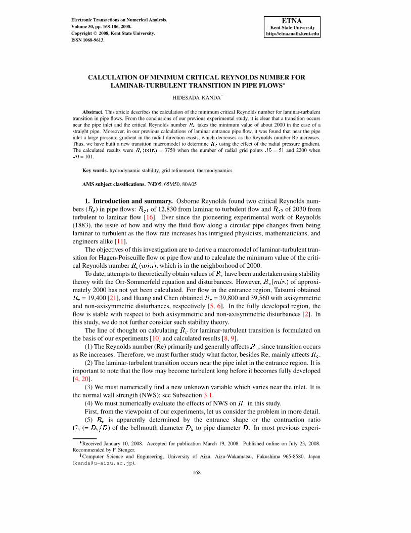
Figures 2.3 through 2.7 show the calculated results of (a) axial pressure drop and (b)pressure distribution in the radial direction. The relationship between the pressure (Q ) andpressure drop ( P'Q ) is P'Q = 0 - Q = - Q , where Q is zero at the inlet.

To verify the accuracy of calculations, the results of calculations are compared with thesmooth curves drawn using Shapiro et al.’s experimental results [17], as shown in Fig. 2.3(a)



174 H. KANDA

TABLE 2.1Grid system, time step ¼¾½ , T-steps, and CPU times.

Re I0/J0 ¼º½ T-steps CPU500 1000/51 0.0001–0.0005 6,000,000 10h 42m

1000 1000/51 0.0001–0.0002 9,000,000 20h 26m2000 1000/51 0.0001–0.0002 9,000,000 22h 34m3000 1000/51 0.0001–0.0002 9,000,000 27h 13m5000 1000/51 0.0001–0.0005 6,000,000 10h 17m

10,000 1000/51 0.0001–0.0005 6,000,000 11h 24m500 1000/101 0.0001–0.0005 6,000,000 24h 54m

1000 1000/101 0.0001–0.0002 8,000,000 26h 27m2000 1000/101 0.0001–0.0002 9,000,000 31h 06m3000 1000/101 0.0001–0.0002 10,000,000 30h 30m5000 1000/101 0.0001–0.0002 10,000,000 49h 39m

10,000 1000/101 0.0001–0.0002 10,000,000 30h 59m

centerline wallexperiment

Pressure Drop

0.01

0.10

1.00

10.00

Downstream Distance (X)0.00001 0.00010 0.00100 0.01000

X=0.00002 X=0.0001X=0.0003 X=0.0005

Pressure

-0.4

-0.3

-0.2

-0.1

0.0

0.1

0.2

Radius (r)0.0 0.1 0.2 0.3 0.4 0.5

FIG. 2.3. (a) Axial pressure drop and (b) pressure distribution in r-direction, Re = 1000.

through 2.7(a), where the diamond and dot symbols denote the calculated results for pressureat the centerline (Q � ) and for pressure at the wall (Q7¿ ), respectively. Near the pipe inlet,the experimental results fall between Q � and Qr¿ and agree well with the computed resultsdownstream.

The major conclusions concerning the radial pressure distribution are as follows. Here,( P'Q ¿ ^¥P'Qr� ) = (Q7��^�Q ¿ ).

(1) It is clear, from Fig. 2.3(a), that at Re = 1000, there is a large difference between P'Q ¿and P'Qr� across the radius of the pipe at 4=¢ CGF CECDC @ , and that this difference decreases as 4increases.

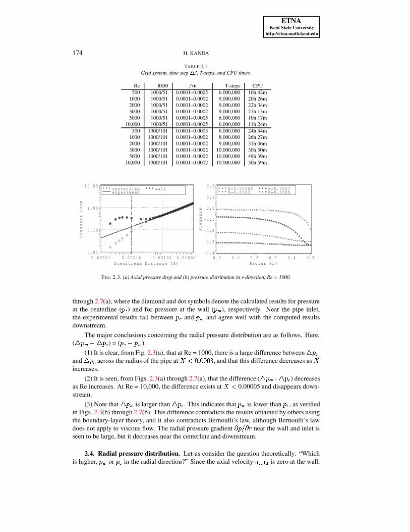
(2) It is seen, from Figs. 2.3(a) through 2.7(a), that the difference ( P'Q ¿ - P'Q7� ) decreasesas Re increases. At Re = 10,000, the difference exists at 4K¢ 0.00005 and disappears down-stream.

(3) Note that P'Q ¿ is larger than P'Q7� . This indicates that Q ¿ is lower than Q7� , as verifiedin Figs. 2.3(b) through 2.7(b). This difference contradicts the results obtained by others usingthe boundary-layer theory, and it also contradicts Bernoulli’s law, although Bernoulli’s lawdoes not apply to viscous flow. The radial pressure gradient

t Q , t x near the wall and inlet isseen to be large, but it decreases near the centerline and downstream.

2.4. Radial pressure distribution. Let us consider the question theoretically: “Whichis higher, Qr¿ or Q � in the radial direction?” Since the axial velocity � �® ° m is zero at the wall,





Pressure Drop

0.01

0.10

1.00

10.00


X=0.00002 X=0.0001X=0.0003 X=0.0005

Pressure

-0.4

-0.3

-0.2

-0.1

0.0

0.1

0.2

Radius (r)0.0 0.1 0.2 0.3 0.4 0.5



Pressure Drop

0.01

0.10

1.00

10.00


X=0.00002 X=0.0001X=0.0003 X=0.0005

Pressure

-0.4

-0.3

-0.2

-0.1

0.0

0.1

0.2

Radius (r)0.0 0.1 0.2 0.3 0.4 0.5


the 5 component of velocity, � , can be linearly approximated as� 0® ° � 3 �� ® ° m V¥� 0® ° � #A 8 >A � �® ° � F(2.11)

From (2.9), (2.10), and (2.11), the vorticity at the wall is simply approximated asu�0® ° m 8À^ t �t x�¶¶¶¶ Á ·ÃÂ 3 � 0® ° �P xÅÄ CUF(2.12)

Substituting (2.12) into (3.2) (see Subsection 3.1) givest Qt x ¶¶¶¶ Á ·$Â 8 ARe

tvu��t 5 ¶¶¶¶ Á ·ÃÂ 3 ARe

tt 5 � � �® ° �P x #(2.13) 3 A

Re� � � � ® ° � ^`� �» � ® ° �A P!57P x � < CGF

Thus, since � � � ® ° � ¢Æ� �» � ® ° � in the entrance region, the normal pressure gradient at thewall becomes negative. Therefore, it is verified from (2.13) that the pressure gradient in theradial direction is negative at the wall of the entrance region.

On the other hand, in the fully developed region, since � � � ® ° � 8?� �» � ® ° � in (2.13), thenormal pressure gradient at the wall becomes 0, thus making the pressure distribution uniformin the radial direction.



176 H. KANDA


Pressure Drop

0.01

0.10

1.00

10.00


X=0.00002 X=0.0001X=0.0003 X=0.0005

Pressure

-0.4

-0.3

-0.2

-0.1

0.0

0.1

0.2

Radius (r)0.0 0.1 0.2 0.3 0.4 0.5



Pressure Drop

0.01

0.10

1.00

10.00


X=0.00002 X=0.0001X=0.0003 X=0.0005

Pressure

-0.4

-0.3

-0.2

-0.1

0.0

0.1

0.2

Radius (r)0.0 0.1 0.2 0.3 0.4 0.5

FIG. 2.7. (a) Axial pressure drop and (b) pressure distribution in r-direction, Re = 10,000.

The velocity distribution in the fully developed region is given by�� x #`8 A l�m { >*^W� x� # � |Ç�(2.14)

where l�m�8�> in dimensionless form. Differentiating (2.14) with respect to x givesu ¡ Á ·$Â 8h^ t �t x ¶¶¶¶ Á ·ÃÂ 8h^ AY� ^ A �� 8 b >� 8Èj �where the dimensionless value of � is 0.5. Thus, the value of

umonotonically decreases

from a large positive value at the leading edge to 8 in the fully developed region.

3. Evaluation of radial pressure gradient.

3.1. Normal pressure gradient at wall. Here, we consider the radial pressure gradientt Q , t x . The dimensionless N-S equation in vector form [3] is written ast �trw ^��_� u 8�^ >A�ÉEÊ-ËEÌ �ÍQ'Vf� � #�^ >Re�� u F(3.1)

Since the velocity vector ��8 C at the wall, the normal component of (3.1) at the wall reducesto t Qt x ¶¶¶¶ Á ·ÃÂ 8 ^ A

Re�Î� u ¡ Á ·ÃÂ 8 A

Re

tUu��t 5 ¶¶¶¶ Á ·$Â F(3.2)



CALCULATION OF MINIMUM CRITICAL REYNOLDS NUMBER 177ÏÑÐÒcÓÔfÕÖf×Ø ÙÚÚÚ

ARe� �� u �ÜÛ ¶¶¶¶ Á ·ÃÂ 8 ^ t Qt 5 ¶¶¶¶ Á ·$ÂA

Re� �Ý� u � Á ¶¶¶¶ Á ·$Â 8 ^ t Qt x ¶¶¶¶ Á ·ÃÂ

Centerline

Wall

Flow

Fluid particlewith vorticity

FIG. 3.1. Directions of curl of vorticity at wall.

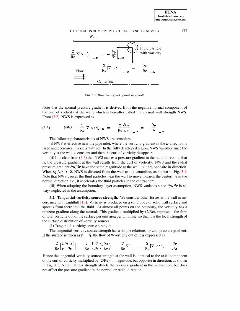
Note that the normal pressure gradient is derived from the negative normal component ofthe curl of vorticity at the wall, which is hereafter called the normal wall strength NWS.From (3.2), NWS is expressed as

NWS Þ ARe�Î� u ¡ Á ·ÃÂ 8 ^ A

Re

tvu �t 5 ¶¶¶¶ Á ·$Â 8 ^ t Qt xJ¶¶¶¶ Á ·ÃÂ F(3.3)

The following characteristics of NWS are considered.(i) NWS is effective near the pipe inlet, where the vorticity gradient in the 5 -direction is

large and decreases inversely with Re. In the fully developed region, NWS vanishes since thevorticity at the wall is constant and then the curl of vorticity disappears.

(ii) It is clear from (3.3) that NWS causes a pressure gradient in the radial direction, thatis, the pressure gradient at the wall results from the curl of vorticity. NWS and the radialpressure gradient

t Q , t x have the same magnitude at the wall, but are opposite in direction.When

t Q , t x ¢ C , NWS is directed from the wall to the centerline, as shown in Fig. 3.1.Note that NWS causes the fluid particles near the wall to move towards the centerline in thenormal direction, i.e., it accelerates the fluid particles in the central core.

(iii) When adopting the boundary-layer assumption, NWS vanishes sincet Q , t x is al-

ways neglected in the assumption.

3.2. Tangential-vorticity source strength. We consider other forces at the wall in ac-cordance with Lighthill [13]. Vorticity is produced on a solid body or solid wall surface andspreads from there into the fluid. At almost all points on the boundary, the vorticity has anonzero gradient along the normal. This gradient, multiplied by (2/Re), represents the flowof total vorticity out of the surface per unit area per unit time, so that it is the local strength ofthe surface distribution of vorticity sources.

(1) Tangential-vorticity source strength.The tangential-vorticity source strength has a simple relationship with pressure gradient.

If the surface is taken as x 8k� , the flow of � -vorticity out of it is expressed as^ ARe ß >x t � x u #t x}à 8 A

Re ß >x tt x�á x t �t x�ârà 8 ARe� � �_8 ^ A

Re� �Ý� u �ÜÛk8 t Qt 5 F

Hence the tangential-vorticity source strength at the wall is identical to the axial componentof the curl of vorticity multiplied by (2/Re) in magnitude, but opposite in direction, as shownin Fig. 3.1. Note that this strength affects the pressure gradient in the 5 -direction, but doesnot affect the pressure gradient in the normal or radial direction.



178 H. KANDA

(2) Normal-vorticity source strength.The normal-vorticity source strength is directly derived under the continuity condition on

u.

The continuity equation foru

in cylindrical coordinates isÌäã±å u Þ >x t � x u Á #t x V >x tvu �t � V tvu�æt7ç 8 CUFFrom the above equation, the normal-vorticity source strength is expressed asA

Re

tt x � x u Á #`8 ^ ARe ß >x tvu��t � V tvu Ût 5 à F

In two dimensions,u Á � u Û � and their derivative with respect to � are all zero. Accordingly,

this normal-vorticity source strength vanishes in the two-dimensional coordinates and affectsnothing.

3.3. Increase in kinetic energy. In the entrance region, the velocity distribution changesfrom uniform at the inlet to parabolic in the fully developed region. The magnitude of theincrease in kinetic energy is considered below.

(i) At the inlet, the velocity profile is uniform: �� C � x #º8èl m F The kinetic energy acrossthe inlet is given by multiplying the flux by its kinetic energy,é Âm Aëê xëìDx�í l m í � >A oGl �m #[8 >j ê o�+ � l ¦m F(3.4)

(ii) In the fully developed region, the velocity has a parabolic distribution (2.14). Ac-cordingly, the kinetic energy is calculated asé Âm ABê x � >A oä#$î A l m ß >J^�� x� # � àrï ¦ ìEx 8 >b ê o�+ � l ¦m F(3.5)

(iii) The increase in kinetic energy (KE 6 ) in the entrance region is obtained by subtract-ing (3.4) from (3.5), which gives

KE 6 8 >b ê o�+ � l ¦m ^ >j ê o�+ � l ¦m 8 >j ê o�+ � l ¦m FThe dimension of this increase in kinetic energy is{ñð�ò� ¦ � � � � ó # ¦ 8 ð�ò � �ó ¦ 8 ð�ò �ó � � ó | FThis unit corresponds to physical power, i.e., energy per second. We define a dimensionlessincrease in kinetic energy per second, KE, as

KE Þ >j ê o�+ � l ¦m>A o�+ � l ¦m 8 ê b 8 CGFÍô j IGF(3.6)

This value of KE = 0.785 is a constant and is independent of Re; thus, KE satisfies thenecessary condition of parameter (a). RW is similarly normalized by (1/2) o�+ � l ¦m ; see Sub-section 4.2.




4. Power done by NWS.

4.1. Variation of enthalpy with pressure. Using the pressure drop (Q � ^`Qr¿ ) in theradial direction, the amount of work WK done by NWS is considered. Here, on the basis ofthermodynamics [12], the variation of enthalpy õ with pressure Q , at a fixed temperature, canbe obtained from the definition õ�8�lkV�Qr� , where l is the internal energy and � is thevolume. For changes in õ , we haveP1õö8�P]lµVKP`�ÍQr�%# FFor most solids and liquids, at a constant temperature, the internal energy l´�0÷ � �%# does notchange as ì lø8 � t lt ÷ � V

ì ÷eV � t lt � � T

ì ��8 C �where ÷ is the temperature. Since the change in volume is rather small, unless the changes inpressure are very large, the change in enthalpy P1õ resulting from a change in pressure P'Qcan be approximated by

WK 8kP1õö3È�ñP'Q F(4.1)

Equation (4.1) can be applied to incompressible flow as well. The unit of �%P'Q is expressedas { � ¦ í ð�ò � ó � >� � 8 ð�ò � �ó � 8 ð�ò � ó � í � | FThis unit, however, is equal to work in physics, and not to power such as KE.

4.2. Power done by NWS. The power RW done by NWS, or the rate of change of thework WK, can be obtained by dividing the work given in (4.1) by period P w , but at this point,the period is not yet known,

RW 8 WKP w 8 �%P'QP w FHere, consider the dimensionless RW. RW is normalized by the same method as KE in (3.6).Lengths, pressure, and time are normalized by + , (1/2) oGl �m , and ��+ , l m # , respectively. Ac-cordingly, the dimensionless RW is expressed as

RW 8 �'P'QP w 8 ùÃú ûqü&úûSý ú+ ¦ í ��> ,BA #poGl �m í �2l m , +þ# 8 ùÃúÜûqü&úûSý ú�n> ,EA #po�+ � l ¦m �where ( 6 ) denotes dimensional quantities.

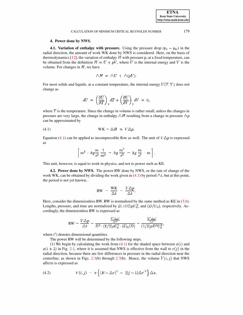
The power RW will be determined by the following steps.(1) We begin by calculating the work from (4.1) for the shaded space between 5��0 �# and5�� V?>/# in Fig. 2.1, where it is assumed that NWS is effective from the wall to x � ¬ # in the

radial direction, because there are few differences in pressure in the radial direction near thecenterline, as shown in Figs. 2.3(b) through 2.7(b). Hence, the volume �ÿ�� ¬ # that NWSaffects is expressed as�ÿ�� 2¬ #g8 ê î ��:^¥P x # � ^ �±� ¬ ^f>X#sP x � � ï P!5 F(4.2)



180 H. KANDA

1

2

J0

Pipe wall

Pipe inlet

Flow

Pipe outlet

J1

J2

R

1

Centerline

j

r

i’ i’+1 i’+2

V1 V2

r r r

r

rR -

FIG. 4.1. Grid system, ¼ �� ¼�� .

Next, the pressure difference in the radial direction is approximated by the differencebetween Q�� 2¬ # and Qr¿N�0 �# :P'Q��0 �2¬ #]89Q��0 �2¬ #�^1Q ¿ �0 �#g8 >A �ÍQ �® ¯ VÝQ � � ® ¯ #(4.3) ^ >b � Q �® ° m V�Q 0® ° � VÝQ � � ® ° m V�Q � � ® ° � # F

(2) The period during which NWS acts on the flow passing along vorticities at �� C #and �0 ÇVk> � � C # is considered. The distance between 5�� # and 5��0 ÃVW>X# is P!5 . The velocitiesat two points �0 � ��>X# and �� qV�> � ��>/# respectively are � 0® ° � and � � � ® ° � . Accordingly, theprovisional period P w � �0 �# may be given by dividing the axial grid space P!5 by the meanvelocity at ¬ 8?��> , P w � �� p#[Þ P!5�� 0� 0® ° �qV¥� � � ® ° ��# 3 P!5� � ��¨� ® ° � FHowever, if this provisional P w � �� # is the correct period, the following inconsistency will beencountered. Two simple cases are taken as examples. First, if the grid aspect ratio is (a)P!5k8 A P x , as shown in Fig. 2.1, the work WK(a) and the power RW(a) for the shadedspace between 5�� p# and 5�� 7V:>/# are expressed as

WK ��ä#g8��'P'Q �(4.4)

RW ��ä#g8 �'P'QP!5� � ��¨� ® ° � 8 �;�'P'Q7#Ç� � ��¨� ® ° �A P x F(4.5)

Next, if the grid aspect ratio is (b) P!5]8 P x and �ÿ>*VT� A 8�� , as shown in Fig. 4.1,the work WK(b) in � is calculated by adding the work in �ÿ> and in � A ,

WK ��#[8È�ÿ>XP'Q$>gV=� A P'Q A 3È�ñP'Q �(4.6)

where it is assumed that P'Q�>�3�P'Q A 3�P'Q . Similarly, the power RW(b) in � is calculatedby adding the power in ��> and in � A ,

RW ��&#g8 �ÿ>XP'Q�>P x� ú � ��¨� ® ° � V � A P'Q AP x� ú � ¦ �¨� ® ° � 3 �;�ñP'Qr#Ã� ú � � ® ° �P x 3 ARW ��ä# �(4.7)




vorticity(i’, J0)

vorticity(i’+1, J0)

vorticity(i’+2, J0)

J0

J1

normal wall strength(i’+1)

normal wallstrength(i’)

Wall

r r

r

r

Centerline

i’ i’+1 i’+2

R -

FIG. 4.2. Balance of NWS and pressure at wall.

where � ú � ��¨� ® ° � 3h� ú � � ® ° � 3À� ú � ¦ �¨� ® ° � . As seen from (4.4) and (4.6), WK(a) andWK(b) are the same. When comparing RW(a) and RW(b) respectively calculated using (4.5)and (4.7), however, the power RW(b) is twice as high as RW(a), although the volume andposition are the same.

To avoid this inconsistency, the following period is required for a general grid system ofP!5þ8W"�P x �0"a8�> � A � @ � F&F�F # :P w �0 �#aÞ P x>A �0� 0® ° � V¥� � � ® ° � # 3 >>A � u��® ° m V u� � � ® ° m # �(4.8)

where, from (2.12),u 0® ° m�8�� ® ° � , P x .

This period is based on the following assumptions.(i) The no-slip condition at the wall means that the fluid particles are not undergoing

translation; however, they are undergoing a rotation. It can be imagined that the wall consistsof an array of marbles that are rotating but remain at the same location at the wall ¬ 8 � C[14].

(ii) The rotation of a fluid particle at the wall yields a vortex and vorticity. Then the curlof vorticity yields NWS from (3.3). The diameter of the vortex of the fluid particle at the wallis P x . Accordingly, NWS is produced per vortex, or per P x .

Figure 4.2 shows the balance between NWS and pressure at the contact surface of¬ 8 CUF I �p� C V ��>/# . For simplicity, the above statement is clarified using (3.2) and (4.9)in discrete form. Setting P!5 to be "�P x ,P'QP x 8 A

ReP uP!5 8 A

Re

u� � � ^ u�P!5 8 ARe

u� ú �Ã� ^ u� ú"�P x8 ARe

>"�P x ß � u ú �Ã� ^ u ú �Ã� » ��#$Vk� u ú �Ã� » �S^ u ú �Ã� » ��#$V í&í�í(4.9) Vñ� u� ú � � ^ u� ú # à 3 ARe"q� u� ú � � ^ u� ú #"�P x 8 A

Re

u� ú � � ^ u� úP x �where it is assumed that the vorticity gradient is linear in a small space between 5��0 �# and5�� ÇV:>/# , i.e.,

u� ú �Ã� ^ u� ú �Ã� » � 3 u� ú �Ã� » � ^ u� ú �Ã� » � 3 í�í&í 3 u� ú � � ^ u� ú .



182 H. KANDA

TABLE 4.1Power (RW) and evaluation criteria at Re = 2000, �� = 51.

c1 c2 c3 c4 �� B��Ç� � ��ë�s��B� � �ä� �/��Ã�� ë��Ç� � �%�±Ü� �/�±�� RW1 0.01 – 1.00 – 0.00029 0.00 1.2782 0.01 – 0.95 – 0.00029 0.09 1.0673 0.01 – 0.90 – 0.00029 0.13 0.8984 0.05 – 1.00 – 0.00016 0.00 1.0855 0.05 – 0.95 – 0.00016 0.10 0.8956 0.05 – 0.90 – 0.00016 0.14 0.7447 – 0.01 1.00 – 0.00041 0.06 1.3028 – 0.01 0.95 – 0.00041 0.16 1.0899 – 0.01 0.90 – 0.00041 0.20 0.917

10 – 0.03 1.00 – 0.00032 0.00 1.28711 – 0.03 0.95 – 0.00032 0.10 1.07612 – 0.03 0.90 – 0.00032 0.13 0.90613 – 0.05 1.00 – 0.00028 0.00 1.27414 – 0.05 0.95 – 0.00028 0.09 1.06415 – 0.05 0.90 – 0.00028 0.13 0.89416 – 0.03 – !n�#"�$ 0.00032 0.28 0.194

TABLE 4.2Power (RW) and evaluation criteria at Re = 2000, �� = 101.

c1 c2 c3 c4 �� ä� �/�� %�±Ü� �/�±�� RW17 0.01 – 1.00 – 0.00024 0.04 1.02918 0.01 – 0.95 – 0.00024 0.13 0.81419 0.01 – 0.90 – 0.00024 0.17 0.67420 0.05 – 1.00 – 0.00013 0.00 0.91221 0.05 – 0.95 – 0.00013 0.12 0.70822 0.05 – 0.90 – 0.00013 0.17 0.57923 – 0.01 1.00 – 0.00029 0.30 1.03924 – 0.01 0.95 – 0.00029 0.31 0.82225 – 0.01 0.90 – 0.00029 0.32 0.68226 – 0.03 1.00 – 0.00026 0.08 1.03527 – 0.03 0.95 – 0.00026 0.17 0.81928 – 0.03 0.90 – 0.00026 0.21 0.67929 – 0.05 1.00 – 0.00024 0.02 1.02930 – 0.05 0.95 – 0.00024 0.13 0.81431 – 0.05 0.90 – 0.00024 0.17 0.67432 – 0.03 – !n�#"�$ 0.00026 0.33 0.087

(3) The power RW(i) for the volume �þ�0 �2¬ # is derived from (4.2), (4.3), and (4.8). Thusthe total power RW is

RW 8&% �ÿ�� 2¬ #�P'Q��0 �2¬ #P w �� # F(4.10)

4.3. Effective region of NWS. In order to calculate the power RW in (4.10), we mustdetermine the effective axial and radial regions of NWS. The effective region is determinedby the following criteria c1–c4. Here,

C Z[Q � �0 �#NZ`Q��0 ��¬ #SZ`Qv¿*�0 �# in the radial direction.Axially: (i) c1 = (Q � ^1Qv¿ ), (ii) c2 = (Qv¿g^!Q � )/Q � .Radially: (iii) c3 = (Q��0 �2¬ #�^1Qr¿ )/(Q � ^1Qv¿�# , (iv) c4 =

u.

The calculated results of RW are listed in Tables 4.1 for � C = 51 and 4.2 for � C = 101.The effective regions of NWS are derived using Tables 4.1 and 4.2, and Fig. 2.4 at Re = 2000.




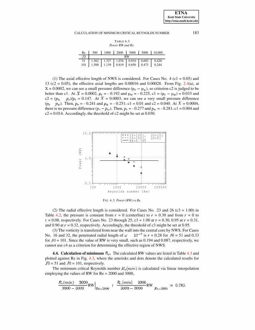
TABLE 4.3Power RW and Re.

Re 500 1000 2000 3000 5000 10,000�� RW51 1.562 1.327 1.076 0.910 0.692 0.420101 1.500 1.139 0.819 0.656 0.473 0.244

(1) The axial effective length of NWS is considered. For Cases No. 4 (c1 = 0.05) and13 (c2 = 0.05), the effective axial lengths are 0.00016 and 0.00028. From Fig. 2.4(a), atX = 0.0002, we can see a small pressure difference (Q � ^1Qr¿ ), so criterion c2 is judged to bebetter than c1. At 4 = 0.0002, Q � = - 0.192 and Qr¿ = - 0.225, c1 = (Q � ^aQr¿ ) = 0.033 andc2 = (Q ¿ ^�Qr� )/Qr� = 0.147. At 4 = 0.0003, we can see a very small pressure difference(Q7�S^]Q ¿ ). Then, Q7� = - 0.241 and Q ¿ = - 0.251; c1 = 0.01 and c2 = 0.040. At 4 = 0.0004,there is no pressure difference (QÇ�r^�Q ¿ ). Then, Q7� = - 0.277 and Q ¿ = - 0.281; c1 = 0.004 andc2 = 0.014. Accordingly, the threshold of c2 might be set at 0.030.

I0=1001, J0=101I0=1001, J0=51KE=0.785

Power (RW)

0.1

1.0

10.0

Reynolds number (Re)100 1000 10000 100000

FIG. 4.3. Power (RW) vs Re.

(2) The radial effective length is considered. For Cases No. 23 and 26 (c3 = 1.00) inTable 4.2, the pressure is constant from x = 0 (centerline) to x = 0.30 and from x = 0 tox = 0.08, respectively. For Cases No. 23 through 25, c3 = 1.00 at x = 0.30, 0.95 at x = 0.31,and 0.90 at x = 0.32, respectively. Accordingly, the threshold of c3 might be set at 0.95.

(3) The vorticity is transfered from near the wall into the central core by NWS. For CasesNo. 16 and 32, the penetrated radial length of

u 89> C »('is x = 0.28 for � C = 51 and 0.33

for � C = 101. Since the value of RW is very small, such as 0.194 and 0.087, respectively, wecannot use c4 as a criterion for determining the effective region of NWS.

4.4. Calculation of minimum �� . The calculated RW values are listed in Table 4.3 andplotted against Re in Fig. 4.3, where the asterisks and dots denote the calculated results for� C = 51 and � C = 101, respectively.

The minimum critical Reynolds number � � �0�1 2"$# is calculated via linear interpolationemploying the values of RW for Re = 2000 and 3000,� � �0�1 2"$#�^`@ CECECABCDCEC ^`@ CECDC RW ¶¶¶ Â M · �smsm¨m V � � �0�1 2"$#�^ ABCDCEC@ CDCEC ^ AECECDC RW ¶¶¶ Â M · ¦ msm¨m 8 CGFÍô j IäF



184 H. KANDA

We thus obtained ��! �"$# of 3750 when � C = 51 and 2200 when � C = 101.

Conclusions. A conceptual macromodel was built to determine ��/�0�1 �"$# for pipe flows,on the basis of the results of our experiments and previous calculations. The calculated resultswere ��/�0�1 �"$# = 3750 when � C = 51 and 2200 when � C = 101.

The model is based on NWS. NWS causes the difference (Q � ^�Qv¿ ) in the radial directionand accelerates fluid particles in the central core. In the entrance region, the velocity profilechanges from a uniform distribution at the pipe inlet to a parabolic one in the fully developedregion. The fluid particles in the central core are accelerated. The magnitude of the requirednondimensional acceleration power is KE = 0.785, which is derived from the difference inkinetic energy between the flow at the inlet and that in the fully developed region.

The occurrence of the transition depends on the acceleration power RW given by NWS:(a) when RW ¢ 0.785, transition takes place;(b) when RW Z 0.785, transition never takes place.

A detailed study of the physical mechanism behind NWS and the occurrence of transitionwill be a future work.

Acknowledgment. We wish to express our sincere appreciation to Emeritus ProfessorF. Stenger of the University of Utah, Professor T. K. DeLillo of Wichita State University, andDr. K. Shimomukai of SGI Japan for useful advice and encouragement, and to the InformationSynergy Center, Tohoku University, for its outstanding computational services.

REFERENCES

[1] R.-Y. CHEN, Flow in the entrance region at low Reynolds numbers, J. Fluids Eng., 95 (1973), pp. 153–158.[2] P. G. DRAZIN AND W. H. REID, Hydrodynamic Stability, Cambridge University Press, 1981, p. 219.[3] S. GOLDSTEIN, Modern Developments in Fluid Dynamics, Vol. 1, Dover, 1965, pp. 97, 297–309.[4] R. A. GRANGER, Fluid Mechanics, Dover, 1995, pp. 481–484.[5] L. M. HUANG AND T. S. CHEN, Stability of the developing laminar pipe flow, Phys. Fluids, 17 (1974),

pp. 245–247.[6] L. M. HUANG AND T. S. CHEN, Stability of developing pipe flow subjected to non-axisymmetric distur-

bances, J. Fluid Mech., 63 (1974), pp. 183–193.[7] H. KANDA, Numerical study of the entrance flow and its transition in a circular pipe, ISAS (Institute of Space

and Astronautical Science), Tokyo, Report No. 626, 1988.[8] H. KANDA, Computerized model of transition in circular pipe flows. Part 2. Calculation of the minimum crit-

ical Reynolds number, ASME (American Society of Mechanical Engineers) FED, 250 (1999), pp. 197–204.

[9] H. KANDA, Laminar-turbulent transition: Calculation of minimum critical Reynolds number in channelflow, RIMS (Research Institute for Mathematical Science, Kyoto Univ.) Kokyuroku, Bessatsu B1, 2007,pp. 199–217.

[10] H. KANDA AND T. YANAGIYA, Hysteresis curve in reproduction of Reynolds’s color-band experiments, J.Fluids Eng., 130 (2008), 051202 (10 pages).

[11] R. R. KERSWELL, Recent progress in understanding the transition to turbulenve in a pipe, Nonlinearity, 18(2005), pp. R17–R44.

[12] D. KONDEPUDI AND I. PRIGOGINE, Modern Thermodynamics, John Wiley & Sons, 1998, pp. 22, 55–56.[13] M. J. LIGHTHILL, Laminar Boundary Layers, L. Rosenhead, ed., Dover, 1988, p. 54.[14] R. L. PANTON, Incompressible Flow, Wiley-Interscience, 1984, p. 323.[15] P. J. ROACHE, Fundamentals of Computational Fluid Dynamics, Hermosa, 1998, pp. 196–200.[16] O. REYNOLDS, An experimental investigation of the circumstances which determine whether the motion of

water shall be direct or sinuous, and of the Law of resistance in parallel channels, Trans. Royal Soc.London, 174 (1883), pp. 935–982.

[17] A. H. SHAPIRO, R. SIEGEL, AND S. J. KLINE, Friction factor in the laminar entry region of a smooth tube,Proc. 2nd Natl. Congr, Appl. Mech., ASME, 1954, pp. 733–741.

[18] K. SHIMOMUKAI AND H. KANDA, Numerical study of normal pressure distribution in entrance flow betweenparallel plates. I. Finite difference calculations, Electron. Trans. Numer. Anal., 23 (2006), pp. 202–218.http://etna.math.kent.edu/vol.23.2006/pp202-218.dir/pp202-218.html.

http://etna.math.kent.edu/vol.23.2006/pp202-218.dir/pp202-218.html




[19] K. SHIMOMUKAI AND H. KANDA, Numerical study of normal pressure distribution in entrance pipe flow,Electron. Trans. Numer. Anal., 30 (2008), pp. 10–25.http://etna.math.kent.edu/vol.30.2008/pp10-25.dir/pp10-25.html.

[20] S. TANEKODA, Fluid Dynamics by Learning from Flow Images (in Japanese), Asakura Publishing Co.,Tokyo, 1993, p. 165.

[21] T. TATSUMI, Stability of the laminar inlet-flow prior to the formation of Poisseuile regime, J. Phy. Soc. ofJapan, 7 (1952), pp. 489–502.

Appendix A.

A.1. Nomenclature.(*)= contraction ratio = + )¤, ++ = pipe diameter = 2 �+ ) = bellmouth diameterõ = enthalpy = l + Q7� , where � is volume = axial point of grid system� C = number of axial grid points¬ = radial point of grid system� C = number of radial grid points

KE = increase in kinetic energy (unit is power); see (3.6)NWS = normal wall strength; see (3.3)Q = pressure = Q 6 , �n�n> ,BA #poGl �m #x = radial coordinate = x 6 , +� = pipe radius = � 6 , + = 0.5Re = Reynolds number = l m + ,*)RW = power done by NWS or rate of change of work; see (4.10)w

= time = ��l m , +þ# w 6÷ = temperature� = axial velocityl m = mean axial velocity at pipe inletl = internal energy� = radial velocity� = velocity vector or volumeWK = work done by NWS5 = axial coordinate = 5 6 , +5 6 = actual axial coordinate4 = axial coordinate = 5 , R R = 5r6 , ��+ R RX#o = fluid densityy

= streamfunction =y 6 , �2l m + � #u

= vorticity = ��+ , l m # u 6� = angle in cylindrical coordinates)= kinematic viscosityP'Q = pressure dropP x = radial grid sizeP!5 = axial grid size

Superscript: � 6 # = dimensional quantity

http://etna.math.kent.edu/vol.30.2008/pp10-25.dir/pp10-25.html



186 H. KANDA

A.2. Flowchart for explicit iteration method.

Start

1) Set initial and boundary conditions

2) CalculateuS�B� � from

uY�, Eq. (2.1), explicit

3) Calculate �y �B� � � � fromu �B� � and �y �B� � , Eq. (2.2), Gauss-Seidel

4) Calculate �u �B� � � � from �y �E� � � � , Eq. (2.2)

5) Check ¡Ç�u �B� � � � -uY�B� � ¡D¢¥£ �

6) Check ¡ yN�B� � -yS� ¡D¢¥£-�

7) Set initial values for pressure, Eq. (2.5)

8) Calculate better pressure, Eq. (2.7)

Check ¡,+ � � - + ¡E¢¥£-¦ , Gauss-Seidel

End

©©

ª

FIG. A.1. Flowchart for explicit iteration method.

Documents

CALCULATION OF MINIMUM CRITICAL REYNOLDS NUMBER …etna.mcs.kent.edu/vol.30.2008/pp168-186.dir/pp168-186.pdf · Osborne Reynolds found two critical Reynolds num-bers ( ) in pipe o