Calculation of Failure Detection Probability on Safety ... · RF. which are not ... We have to consider calibration inaccuracy, residual . ... described by uncertainty-offsets which

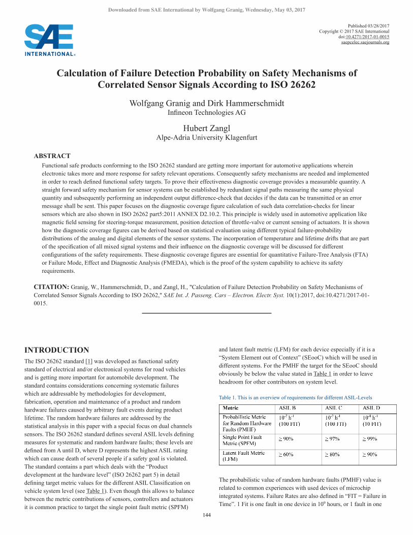
INTRODUCTIONThe ISO 26262 standard [1] was developed as functional safety standard of electrical and/or electronical systems for road vehicles and is getting more important for automobile development. The standard contains considerations concerning systematic failures which are addressable by methodologies for development, fabrication, operation and maintenance of a product and random hardware failures caused by arbitrary fault events during product lifetime. The random hardware failures are addressed by the statistical analysis in this paper with a special focus on dual channels sensors. The ISO 26262 standard defines several ASIL levels defining measures for systematic and random hardware faults; these levels are defined from A until D, where D represents the highest ASIL rating which can cause death of several people if a safety goal is violated. The standard contains a part which deals with the “Product development at the hardware level” (ISO 26262 part 5) in detail defining target metric values for the different ASIL Classification on vehicle system level (see Table 1). Even though this allows to balance between the metric contributions of sensors, controllers and actuators it is common practice to target the single point fault metric (SPFM)

and latent fault metric (LFM) for each device especially if it is a “System Element out of Context” (SEooC) which will be used in different systems. For the PMHF the target for the SEooC should obviously be below the value stated in Table 1 in order to leave headroom for other contributors on system level.

Table 1. This is an overview of requirements for different ASIL-Levels

The probabilistic value of random hardware faults (PMHF) value is related to common experiences with used devices of microchip integrated systems. Failure Rates are also defined in “FIT = Failure in Time”. 1 Fit is one fault in one device in 109 hours, or 1 fault in one

Calculation of Failure Detection Probability on Safety Mechanisms of Correlated Sensor Signals According to ISO 26262

Wolfgang Granig and Dirk HammerschmidtInfineon Technologies AG

Hubert ZanglAlpe-Adria University Klagenfurt

ABSTRACTFunctional safe products conforming to the ISO 26262 standard are getting more important for automotive applications wherein electronic takes more and more response for safety relevant operations. Consequently safety mechanisms are needed and implemented in order to reach defined functional safety targets. To prove their effectiveness diagnostic coverage provides a measurable quantity. A straight forward safety mechanism for sensor systems can be established by redundant signal paths measuring the same physical quantity and subsequently performing an independent output difference-check that decides if the data can be transmitted or an error message shall be sent. This paper focuses on the diagnostic coverage figure calculation of such data correlation-checks for linear sensors which are also shown in ISO 26262 part5:2011 ANNEX D2.10.2. This principle is widely used in automotive application like magnetic field sensing for steering-torque measurement, position detection of throttle-valve or current sensing of actuators. It is shown how the diagnostic coverage figures can be derived based on statistical evaluation using different typical failure-probability distributions of the analog and digital elements of the sensor systems. The incorporation of temperature and lifetime drifts that are part of the specification of all mixed signal systems and their influence on the diagnostic coverage will be discussed for different configurations of the safety requirements. These diagnostic coverage figures are essential for quantitative Failure-Tree Analysis (FTA) or Failure Mode, Effect and Diagnostic Analysis (FMEDA), which is the proof of the system capability to achieve its safety requirements.

CITATION: Granig, W., Hammerschmidt, D., and Zangl, H., "Calculation of Failure Detection Probability on Safety Mechanisms of Correlated Sensor Signals According to ISO 26262," SAE Int. J. Passeng. Cars – Electron. Electr. Syst. 10(1):2017, doi:10.4271/2017-01-0015.

Published 03/28/2017Copyright © 2017 SAE International

doi:10.4271/2017-01-0015saepcelec.saejournals.org

144

Downloaded from SAE International by Wolfgang Granig, Wednesday, May 03, 2017

http://dx.doi.org/10.4271/2017-01-0015

http://saepcelec.saejournals.org/

hour at 109 devices. Standards exist which define a FIT-rate related to a certain chip-area. These standard base failure rates are often taken as guideline for comparison of different integrated solutions of independent of manufacturer’s field data (see Table 2). Considerations on the application of the ISO 26262 on semiconductor components for the use in automotive systems can be found in ISO/PAS19451 [4].

Table 2. This is an overview of different base failure rates for semiconductor products used in SPFM and LFM calculations.

The possible hardware faults can be separated in several classes. An explanation including defined variables which are used in following equations can be seen in Table 3. The contribution to the overall fault rate is expressed in Equation 1.

(1)

The Single-Point Fault Metric (SPFM) can be calculated according to Equation 2 considering Single point Faults λSPF directly violating the safety goal uncovered by any safety mechanism and residual faults λRF which are not detected by safety mechanisms.

(2)

The latent Fault Metric (LFM) can be calculated according to Equation 3 using latent multi-point fault rate λMPF which considers faults which are not directly violating the safety goal, but if a second fault occurs subsequently it may be elevated by the undetected first fault to violate the safety requirement. For this calculation the single point faults and residual faults must be excluded, therefore λSPF and λRF are subtracted from the overall failure rate λ

(3)

The diagnostic coverage KDC,RF of a safety mechanism detecting a fault of a hardware-part is expressed in percentage using the residual failure-rate according to Equation 4.

(4)

The same diagnostic coverage can be calculated for the latent faults. The latent fault diagnostic coverage KDC,MPF,L expressed in percentage can be calculated according to Equation 5.

(5)

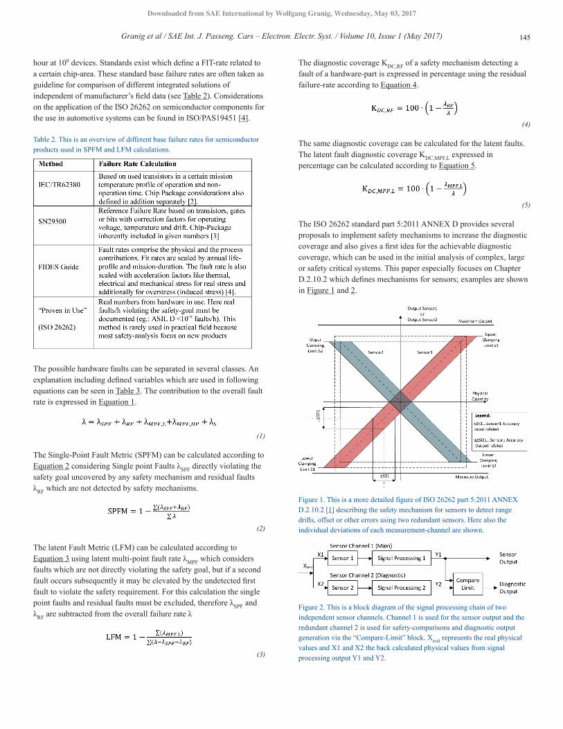
The ISO 26262 standard part 5:2011 ANNEX D provides several proposals to implement safety mechanisms to increase the diagnostic coverage and also gives a first idea for the achievable diagnostic coverage, which can be used in the initial analysis of complex, large or safety critical systems. This paper especially focuses on Chapter D.2.10.2 which defines mechanisms for sensors; examples are shown in Figure 1 and 2.

Figure 1. This is a more detailed figure of ISO 26262 part 5:2011 ANNEX D.2.10.2 [1] describing the safety mechanism for sensors to detect range drifts, offset or other errors using two redundant sensors. Here also the individual deviations of each measurement-channel are shown.

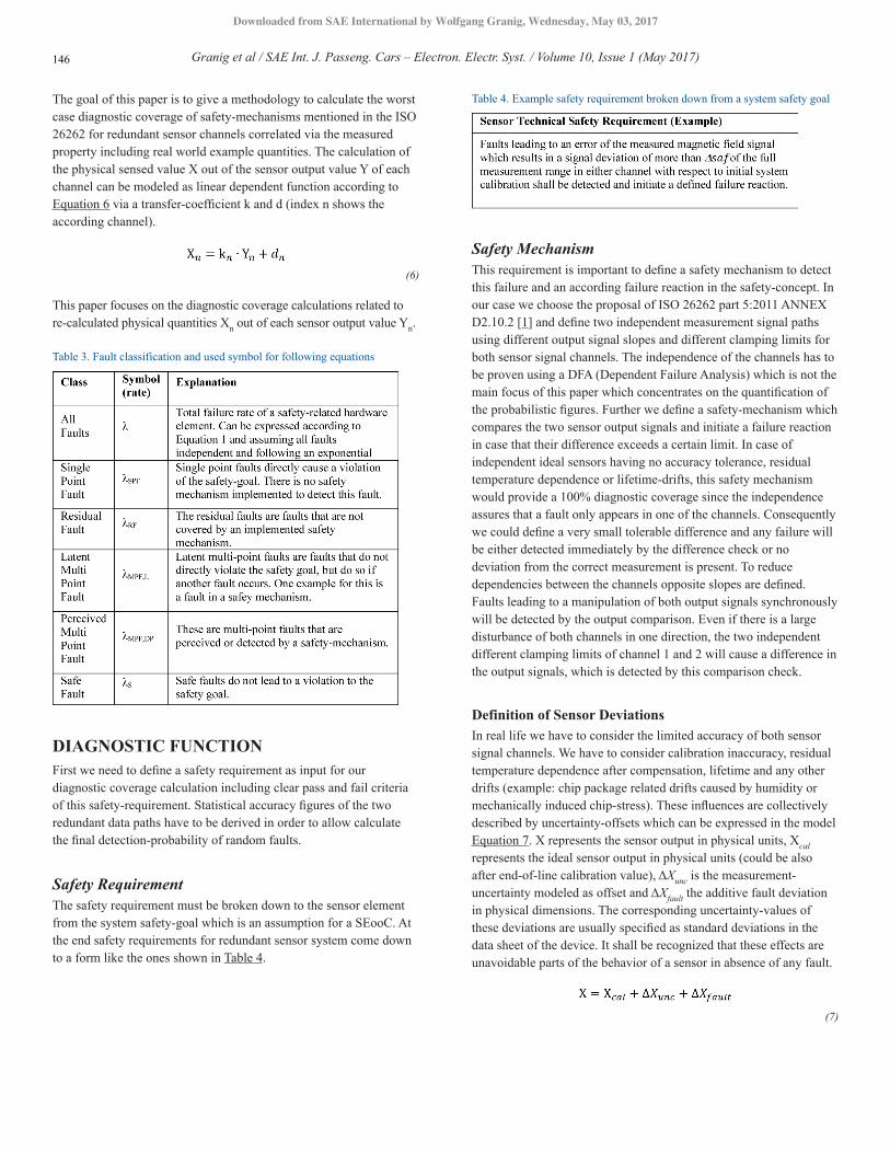
Figure 2. This is a block diagram of the signal processing chain of two independent sensor channels. Channel 1 is used for the sensor output and the redundant channel 2 is used for safety-comparisons and diagnostic output generation via the “Compare-Limit” block. Xreal represents the real physical values and X1 and X2 the back calculated physical values from signal processing output Y1 and Y2.

Granig et al / SAE Int. J. Passeng. Cars – Electron. Electr. Syst. / Volume 10, Issue 1 (May 2017) 145


The goal of this paper is to give a methodology to calculate the worst case diagnostic coverage of safety-mechanisms mentioned in the ISO 26262 for redundant sensor channels correlated via the measured property including real world example quantities. The calculation of the physical sensed value X out of the sensor output value Y of each channel can be modeled as linear dependent function according to Equation 6 via a transfer-coefficient k and d (index n shows the according channel).

(6)

This paper focuses on the diagnostic coverage calculations related to re-calculated physical quantities Xn out of each sensor output value Yn.

Table 3. Fault classification and used symbol for following equations

DIAGNOSTIC FUNCTIONFirst we need to define a safety requirement as input for our diagnostic coverage calculation including clear pass and fail criteria of this safety-requirement. Statistical accuracy figures of the two redundant data paths have to be derived in order to allow calculate the final detection-probability of random faults.

Safety RequirementThe safety requirement must be broken down to the sensor element from the system safety-goal which is an assumption for a SEooC. At the end safety requirements for redundant sensor system come down to a form like the ones shown in Table 4.

Table 4. Example safety requirement broken down from a system safety goal

Safety MechanismThis requirement is important to define a safety mechanism to detect this failure and an according failure reaction in the safety-concept. In our case we choose the proposal of ISO 26262 part 5:2011 ANNEX D2.10.2 [1] and define two independent measurement signal paths using different output signal slopes and different clamping limits for both sensor signal channels. The independence of the channels has to be proven using a DFA (Dependent Failure Analysis) which is not the main focus of this paper which concentrates on the quantification of the probabilistic figures. Further we define a safety-mechanism which compares the two sensor output signals and initiate a failure reaction in case that their difference exceeds a certain limit. In case of independent ideal sensors having no accuracy tolerance, residual temperature dependence or lifetime-drifts, this safety mechanism would provide a 100% diagnostic coverage since the independence assures that a fault only appears in one of the channels. Consequently we could define a very small tolerable difference and any failure will be either detected immediately by the difference check or no deviation from the correct measurement is present. To reduce dependencies between the channels opposite slopes are defined. Faults leading to a manipulation of both output signals synchronously will be detected by the output comparison. Even if there is a large disturbance of both channels in one direction, the two independent different clamping limits of channel 1 and 2 will cause a difference in the output signals, which is detected by this comparison check.

Definition of Sensor DeviationsIn real life we have to consider the limited accuracy of both sensor signal channels. We have to consider calibration inaccuracy, residual temperature dependence after compensation, lifetime and any other drifts (example: chip package related drifts caused by humidity or mechanically induced chip-stress). These influences are collectively described by uncertainty-offsets which can be expressed in the model Equation 7. X represents the sensor output in physical units, Xcal represents the ideal sensor output in physical units (could be also after end-of-line calibration value), ΔXunc is the measurement-uncertainty modeled as offset and ΔXfault the additive fault deviation in physical dimensions. The corresponding uncertainty-values of these deviations are usually specified as standard deviations in the data sheet of the device. It shall be recognized that these effects are unavoidable parts of the behavior of a sensor in absence of any fault.

(7)

Granig et al / SAE Int. J. Passeng. Cars – Electron. Electr. Syst. / Volume 10, Issue 1 (May 2017)146


To fulfill the safety requirement the output-deviation to the ideal transfer-function is not allowed to be larger than the limit Δsaf defined in the safety-requirement coming from customers or from a safety architecture according to Equation 8 with Δsaf representing the safety requirement limit. Obviously the effect of the deviations defined in Equation 7 has to be below the limit that infringes the safety criterion. A visualization of this requirement is also shown in the Venn-diagram in Figure 3 [5].

(8)

Figure 3. This is a Venn-diagram of all sensor output possibilities. If the output value-deviation is within the specification limit the output values are ok (X_ok). If the output-value deviation is larger than the specification limit but lower than the safety limit these faults are safe (X_fail_safe). The lastpossibility is an output value-deviation exceeding the safety limit (X_fail_viol).

Definition of Sensor Safety Mechanism DeviationsTo detect this deviation from the main sensor channel output X1 a second redundant sensor X2 (Sensor 2 shown in Figure 1) is used to measure the difference dX of the two sensor outputs as shown in Figure 1, 2 and Equation 9. In case the difference of the measurements delivered by both channels exceeds a safety-mechanism-limit threshold (dsml) this should be indicated by a safety reaction. For an initial approach the threshold of this safety-mechanism limit is set equally to the safety limit (dssml: = Δsaf). Equation 10 shows that inserting Equation 7 into Equation 9 results in dX only depending on the sensor uncertainties and faults.

(9)

(10)

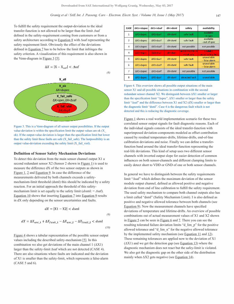
Figure 4 shows a tabular representation of the possible sensor output values including the described safety-mechanism [5]. In this combination we also get deviations of the main channel 1 (ΔX1) larger than the safety-limit Δsaf which are not detected (CASE 4). There are also situations where faults are indicated and the deviation of X1 is smaller than the safety-limit, which represents a false-alarm (CASE 5 and 6).

Figure 4. This overview shows all possible output situations of the main sensor X1 and all possible situations in combination with the second redundant sensor channel X2. We distinguish between ΔX1 smaller or larger than the specification limit “Δspec”, ΔX1 smaller or larger than the safety limit “Δsaf” and the difference between X1 and X2 (dX) smaller or larger than the diagnostic limit “dsml”. Case 4 is the dangerous fault which is not detected and this is reducing the diagnostic coverage.

Figure 1 shows a real world implementation scenario for these two correlated sensor output signals for fault diagnostic reasons. Each of the individual signals consists of the ideal transfer-function with superimposed deviation-components modeled as offset contribution caused by residual temperature-drifts, lifetime-drifts, end-of-line calibration deviations and noise. Finally we can define a transfer-function band around the ideal transfer-function representing the real-life deviations. This kind of setup uses two different sensor channels with inverted output slope for easier detection of common influences on both sensor-channels and different clamping limits to easily detect short to VDD or GND of one or both sensor channels.

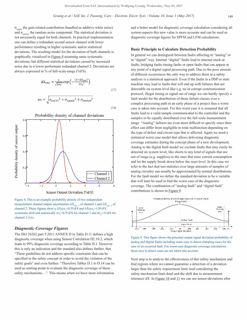
In general we have to distinguish between the safety requirements limit “Δsaf” which defines the maximum deviation of the sensor module output channel, defined as allowed positive and negative deviation from end of line calibration to fulfill the safety requirement. The used safety mechanism to compare both channel outputs also has a limit called “dsml” (Safety Mechanism Limit). I is also defined as positive and negative allowed tolerance between both channels (see Equation 9). Now the measurement channels have specified deviations of temperature and lifetime-drifts. An overview of possible combinations out of actual measurement values of X1 and X2 shown in Figure 5 can be seen in Figure 6 and 7. There you can see the resulting tolerated failure deviation limits “d_lim_p” for the positive allowed tolerance and “d_lim_n” for the negative allowed tolerance by the implemented safety mechanism (see Equation 11 and 12). These remaining tolerances are applied now to the deviation of X1 (ΔX1) and we get the detection gap (see Equation 13) where the diagnostic mechanism does not react but the safey-limit is violated. We also get the diagnostic gap on the other side of the distribution mainly when ΔX2 gets negative (see Equation 14).



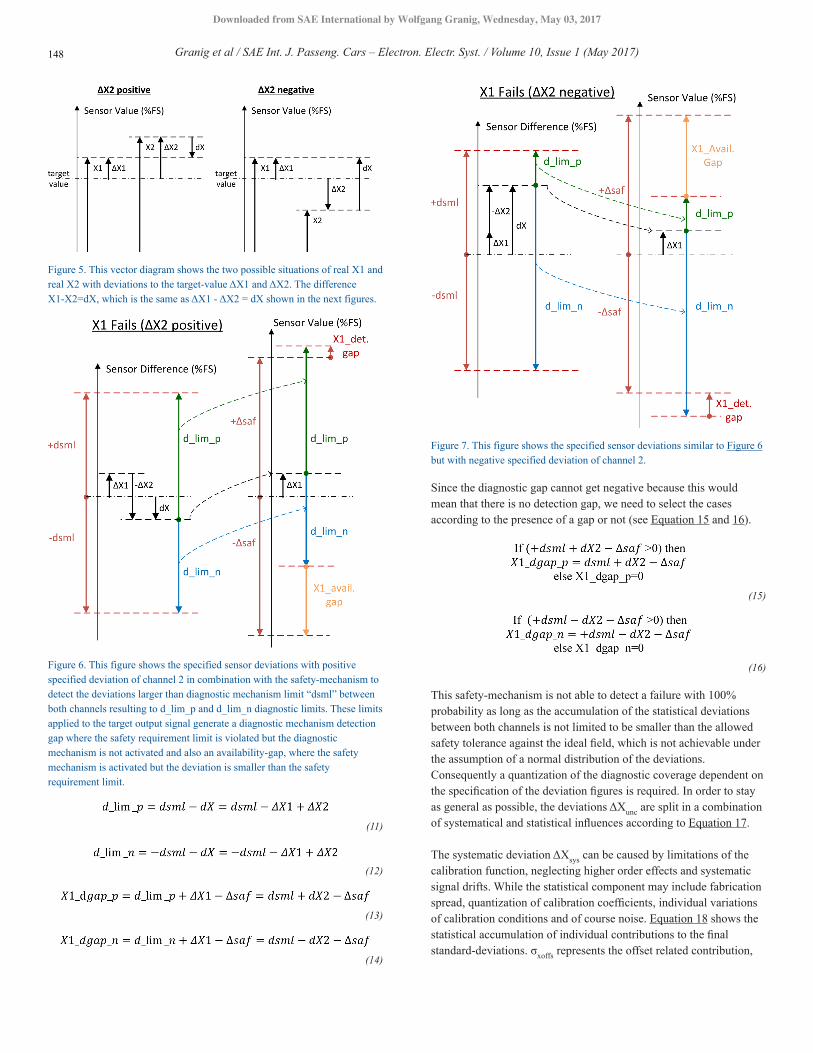
Figure 5. This vector diagram shows the two possible situations of real X1 and real X2 with deviations to the target-value ΔX1 and ΔX2. The difference X1-X2=dX, which is the same as ΔX1 - ΔX2 = dX shown in the next figures.

Figure 6. This figure shows the specified sensor deviations with positive specified deviation of channel 2 in combination with the safety-mechanism to detect the deviations larger than diagnostic mechanism limit “dsml” between both channels resulting to d_lim_p and d_lim_n diagnostic limits. These limits applied to the target output signal generate a diagnostic mechanism detection gap where the safety requirement limit is violated but the diagnostic mechanism is not activated and also an availability-gap, where the safety mechanism is activated but the deviation is smaller than the safety requirement limit.

(11)

(12)

(13)

(14)

Figure 7. This figure shows the specified sensor deviations similar to Figure 6 but with negative specified deviation of channel 2.

Since the diagnostic gap cannot get negative because this would mean that there is no detection gap, we need to select the cases according to the presence of a gap or not (see Equation 15 and 16).

(15)

(16)

This safety-mechanism is not able to detect a failure with 100% probability as long as the accumulation of the statistical deviations between both channels is not limited to be smaller than the allowed safety tolerance against the ideal field, which is not achievable under the assumption of a normal distribution of the deviations. Consequently a quantization of the diagnostic coverage dependent on the specification of the deviation figures is required. In order to stay as general as possible, the deviations ΔXunc are split in a combination of systematical and statistical influences according to Equation 17.

The systematic deviation ΔXsys can be caused by limitations of the calibration function, neglecting higher order effects and systematic signal drifts. While the statistical component may include fabrication spread, quantization of calibration coefficients, individual variations of calibration conditions and of course noise. Equation 18 shows the statistical accumulation of individual contributions to the final standard-deviations. σxoffs represents the offset related contribution,



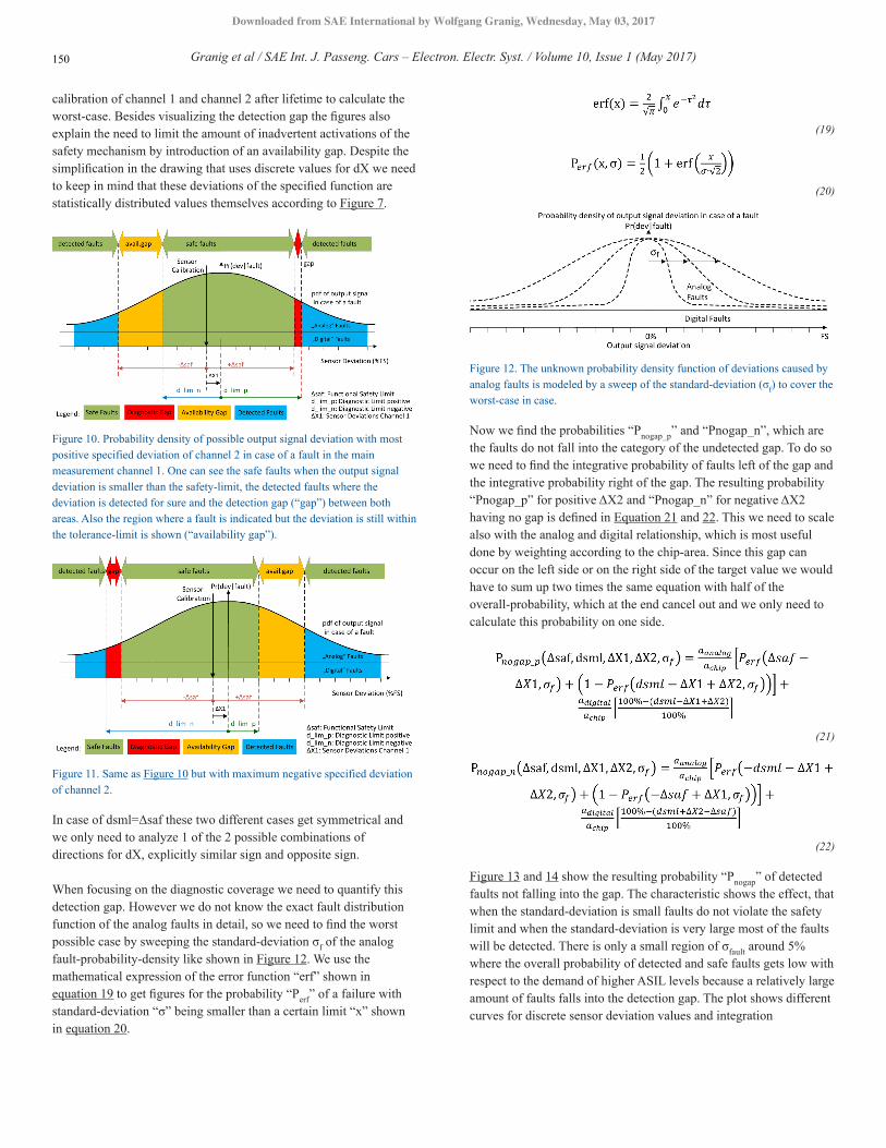
σxgain the gain related contribution (handled as additive white noise) and σxnoise the random noise component. The statistical deviation is not necessarily equal for both channels. In practical implementation one can define a redundant second sensor channel with lower performance resulting in higher systematic and/or statistical deviations. The resulting model for the deviation of both channels is graphically visualized in Figure 8 assuming same systematic deviations, but different statistical deviations caused by increased noise due to a lower performant redundant channel 2. Deviations are always expressed in % of full-scale-range (%FS).

(17)

(18)

Figure 8. This is an example probability density of two independent measurement channel output uncertainties ΔXunc_1.of channel 1 and ΔXunc_2 of channel 2. These figures show a ΔXsys1=0.5%FS and ΔXsys2=1.0%FS systematic drift and statistically σx1=0.5%FS for channel 1 and σx2=1%FS for channel 2 (1σ).

Diagnostic Coverage FiguresThe ISO 26262 part 5:2011 ANNEX D in Table D.11 defines a high diagnostic coverage when using Sensor Correlation D2.10.2, which leads to 99% diagnostic coverage according to Table D.1. However this is only an indication and the standard also defines further, that “These guidelines do not address specific constraints that can be specified in the safety concept in order to avoid the violation of the safety goals” and even further: “Therefore Tables D.1 to D.14 can be used as starting-point to evaluate the diagnostic coverage of these safety mechanisms…”. This means when we have more information

and a better model for diagnostic coverage calculation considering all system-aspects this new value is more accurate and can be used as diagnostic coverage figures for SPFM and LFM calculations.

Basic Principle to Calculate Detection ProbabilityIn general we can distinguish between faults affecting in “analog” or in “digital” way. Internal “digital” faults lead to internal stuck-at faults, bridging faults timing faults or open faults that can appear at any point of a digital signal processing path. Due to the poor amount of different occurrences the only way to address them in a safety analysis is a statistical approach. Even if the faults in a DSP or state machine may lead to faults that will end up with failures that are detectable on system level like e.g. no or corrupt communication protocol, illegal timing or signal out of range we can hardly specify a fault model for the distribution of those failure classes over a complex processing path in an early phase of a project thus a worst case is taken into account. For this worst case it is assumed that all faults lead to a valid sample communicated to the controller and the samples to be equally distributed over the full scale measurement range. “Analog” failures are even more difficult to specify since their effect can differ from negligible to total malfunction depending on the type of defect and circuit type that is affected. Again we need a statistical worst case model that allows delivering diagnostic coverage estimates during the concept phase of a new development. Analog to the digital fault model we exclude faults that may easily be detected on system level, like shorts to any kind of signals that are out of range (e.g. supplies) or the ones that raise current consumption and let the supply break down below the reset level. In this case we refer to the fact that test statistics over large amounts of samples of analog circuitry can usually be approximated by normal distributions. For the fault model we define the standard deviation to be a variable that will later be used to find the worst case of the diagnostic coverage. The combination of “analog fault” and “digital fault” contributions is shown in Figure 9.

Figure 9. This figure shows the potential output signal deviation probability of analog and digital faults including some easy to detect clamping-cases for the case of an occurred fault. For worst-case diagnostic coverage calculations these easy to detect cases are not taken into account.

Next step is to analyze the effectiveness of this safety mechanism and find regions where we cannot guarantee a detection of a deviation larger than the safety requirement limit Δsaf considering the safety-mechanism limit dsml and the shift due to measurement tolerance dX. In Figure 10 and 11 we can see sensor-deviations after



calibration of channel 1 and channel 2 after lifetime to calculate the worst-case. Besides visualizing the detection gap the figures also explain the need to limit the amount of inadvertent activations of the safety mechanism by introduction of an availability gap. Despite the simplification in the drawing that uses discrete values for dX we need to keep in mind that these deviations of the specified function are statistically distributed values themselves according to Figure 7.

Figure 10. Probability density of possible output signal deviation with most positive specified deviation of channel 2 in case of a fault in the main measurement channel 1. One can see the safe faults when the output signal deviation is smaller than the safety-limit, the detected faults where the deviation is detected for sure and the detection gap (“gap”) between both areas. Also the region where a fault is indicated but the deviation is still within the tolerance-limit is shown (“availability gap”).

Figure 11. Same as Figure 10 but with maximum negative specified deviation of channel 2.

In case of dsml=Δsaf these two different cases get symmetrical and we only need to analyze 1 of the 2 possible combinations of directions for dX, explicitly similar sign and opposite sign.

When focusing on the diagnostic coverage we need to quantify this detection gap. However we do not know the exact fault distribution function of the analog faults in detail, so we need to find the worst possible case by sweeping the standard-deviation σf of the analog fault-probability-density like shown in Figure 12. We use the mathematical expression of the error function “erf” shown in equation 19 to get figures for the probability “Perf” of a failure with standard-deviation “σ” being smaller than a certain limit “x” shown in equation 20.

(19)

(20)

Figure 12. The unknown probability density function of deviations caused by analog faults is modeled by a sweep of the standard-deviation (σf) to cover the worst-case in case.

Now we find the probabilities “Pnogap_p” and “Pnogap_n”, which are the faults do not fall into the category of the undetected gap. To do so we need to find the integrative probability of faults left of the gap and the integrative probability right of the gap. The resulting probability “Pnogap_p” for positive ΔX2 and “Pnogap_n” for negative ΔX2 having no gap is defined in Equation 21 and 22. This we need to scale also with the analog and digital relationship, which is most useful done by weighting according to the chip-area. Since this gap can occur on the left side or on the right side of the target value we would have to sum up two times the same equation with half of the overall-probability, which at the end cancel out and we only need to calculate this probability on one side.

(21)

(22)

Figure 13 and 14 show the resulting probability “Pnogap” of detected faults not falling into the gap. The characteristic shows the effect, that when the standard-deviation is small faults do not violate the safety limit and when the standard-deviation is very large most of the faults will be detected. There is only a small region of σfault around 5% where the overall probability of detected and safe faults gets low with respect to the demand of higher ASIL levels because a relatively large amount of faults falls into the detection gap. The plot shows different curves for discrete sensor deviation values and integration



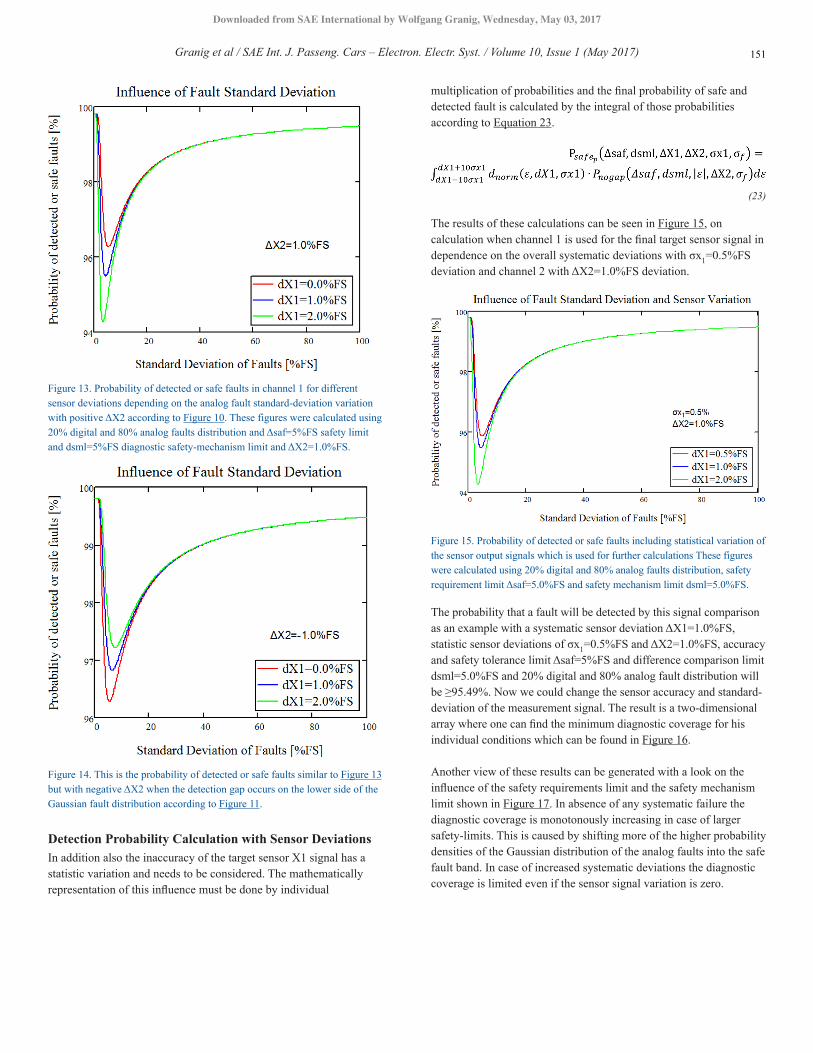
Figure 13. Probability of detected or safe faults in channel 1 for different sensor deviations depending on the analog fault standard-deviation variation with positive ΔX2 according to Figure 10. These figures were calculated using 20% digital and 80% analog faults distribution and Δsaf=5%FS safety limit and dsml=5%FS diagnostic safety-mechanism limit and ΔX2=1.0%FS.

Figure 14. This is the probability of detected or safe faults similar to Figure 13 but with negative ΔX2 when the detection gap occurs on the lower side of the Gaussian fault distribution according to Figure 11.

Detection Probability Calculation with Sensor DeviationsIn addition also the inaccuracy of the target sensor X1 signal has a statistic variation and needs to be considered. The mathematically representation of this influence must be done by individual

multiplication of probabilities and the final probability of safe and detected fault is calculated by the integral of those probabilities according to Equation 23.

(23)

The results of these calculations can be seen in Figure 15, on calculation when channel 1 is used for the final target sensor signal in dependence on the overall systematic deviations with σx1=0.5%FS deviation and channel 2 with ΔX2=1.0%FS deviation.

Figure 15. Probability of detected or safe faults including statistical variation of the sensor output signals which is used for further calculations These figures were calculated using 20% digital and 80% analog faults distribution, safety requirement limit Δsaf=5.0%FS and safety mechanism limit dsml=5.0%FS.

The probability that a fault will be detected by this signal comparison as an example with a systematic sensor deviation ΔX1=1.0%FS, statistic sensor deviations of σx1=0.5%FS and ΔX2=1.0%FS, accuracy and safety tolerance limit Δsaf=5%FS and difference comparison limit dsml=5.0%FS and 20% digital and 80% analog fault distribution will be ≥95.49%. Now we could change the sensor accuracy and standard-deviation of the measurement signal. The result is a two-dimensional array where one can find the minimum diagnostic coverage for his individual conditions which can be found in Figure 16.

Another view of these results can be generated with a look on the influence of the safety requirements limit and the safety mechanism limit shown in Figure 17. In absence of any systematic failure the diagnostic coverage is monotonously increasing in case of larger safety-limits. This is caused by shifting more of the higher probability densities of the Gaussian distribution of the analog faults into the safe fault band. In case of increased systematic deviations the diagnostic coverage is limited even if the sensor signal variation is zero.



Figure 16. Diagnostic coverage calculations including statistical variation of the target sensor signal accuracy and systematic sensor error. These figures were calculated using 20% digital and 80% analog faults distribution and 5% safety as well as diagnostic limit.

Figure 17. Diagnostic coverage calculations including systematic and statistical variation of the sensor signals accuracy, safety- and diagnostic limit Δsaf=dsml. These figures were calculated using 20% digital and 80% analog faults distribution.

Availability Gap

Non Availability Caused by Safe-Faults in Channel 1Depending on the combination and directions of the sensor drift in both channels the detection gap appears on one side outside the safe fault band. It can also be seen from Figure 10 and 11 that a gap for the availability in case of a false alarm appears on the opposite side inside the safe fault band. Due to the symmetry of the Gaussian probability density function it will lead to higher probabilities to fall into the availability gap compared to the detection gap. In contradiction to the safety-gap we want to know what is the probability of a false-alarm in case of a safe fault? This means, when is the sensor output deviation smaller than the safety-limit, and a failure is inadvertently indicated? Equation 24 and 25 express the according availability gap separated for negative and positive ΔX2.

Equation 26 and 27 again resolve the cases where this availability gap becomes negative which means that there is no availability-gap and sets the according value to zero. In case of dsml=Δsaf again this availability gap occurs on both sides of the distribution function symmetrically like the diagnostic gap.

(24)

(25)

(26)

(27)

This fault alarm-rate in case of a safe-fault of channel 1is calculated in Equation 28 for ΔX2>0 and Equation 29 for ΔX2<0 with Δsaf representing the safety requirement limit, dsml the safety mechanism limit, ΔX1and ΔX2 the according systematic sensor deviations and σf the varying standard-deviation of the modeled analog faults.

(28)

(29)

Here again the fault standard-deviation is changed to get the impact of different fault variations to the false alarm rate. To include also the sensor output spread we need to multiply the output spread again with the false-alarm probability individually and integrate the results according to Equation 30. The case for ΔX2<0 is calculated in the same manner, but as mentioned if dsml=Δsaf then these distributions are symmetrically.

(30)

The results of this superposition of sensor variation and potential false-alarm rate calculations can be seen in Figure 18. One can recognize that the worst case false-alarm-rate occurs when the standard-deviation of the analog faults between 5%FS and 10%FS. This extreme case is similar to the diagnostic gap only with probabilities near zero instead of 100%.



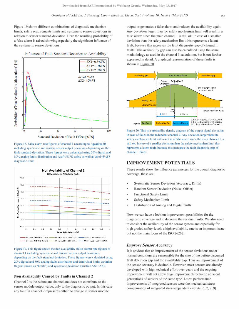
Figure 19 shows different combinations of diagnostic mechanism limits, safety requirements limits and systematic sensor deviations in relation to sensor standard-deviation. Here the resulting probability of a false alarm is raised showing especially the significant influence of the systematic sensor deviations.

Figure 18. False alarm rate figures of channel 1 according to Equation 30 including systematic and random sensor output deviations depending on the fault standard-deviation. These figures were calculated using 20% digital and 80% analog faults distribution and Δsaf=5%FS safety as well as dsml=5%FS diagnostic limit.

Figure 19. This figure shows the non-availability (false alarm) rate figures of channel 1 including systematic and random sensor output deviations depending on the fault standard-deviation. These figures were calculated using 20% digital and 80% analog faults distribution and dsml=Δsaf limits variation (legend shown as “limits”) and systematic deviation variation ΔX1=ΔX2.

Non Availability Caused by Faults in Channel 2Channel 2 is the redundant channel and does not contribute to the sensor module output value, only to the diagnostic output. In this case any fault in channel 2 represents either no change in sensor module

output or generates a false alarm and reduces the availability again. Any deviation larger than the safety mechanism limit will result in a false alarm since the main channel 1 is still ok. In case of a smaller deviation than the safety mechanism limit this represents a latent fault, because this increases the fault diagnostic gap of channel 1 faults. This availability gap can also be calculated using the same methodology as used in the channel 1 calculation, but is not further expressed in detail. A graphical representation of these faults is shown in Figure 20.

Figure 20. This is a probability density diagram of the output signal deviation in case of faults in the redundant channel 2. Any deviation larger than the safety mechanism limit will result in a false alarm since the main channel 1 is still ok. In case of a smaller deviation than the safety mechanism limit this represents a latent fault, because this increases the fault diagnostic gap of channel 1 faults.

IMPROVEMENT POTENTIALSThese results show the influence parameters for the overall diagnostic coverage, these are:

• Systematic Sensor Deviation (Accuracy, Drifts) • Random Sensor Deviation (Noise, Offset) • Functional Safety Limit • Safety Mechanism Limit • Distribution of Analog and Digital faults

Now we can have a look on improvement possibilities for the diagnostic coverage and to decrease the residual faults. We also need to consider the availability of the sensor system and especially for high graded safety-levels a high availability rate is an important issue but not the main focus of the ISO 26262.

Improve Sensor AccuracyIt is obvious that an improvement of the sensor deviations under normal conditions are responsible for the size of the before discussed fault detection gap and the availability gap. Thus an improvement of the sensor accuracy is desirable. However, most sensors are already developed with high technical effort over years and the ongoing improvement will not allow huge improvements between adjacent generations of sensors of the same type. Latest performance improvements of integrated sensors were the mechanical stress-compensation of integrated stress-dependent circuits [6, 7, 8, 9].



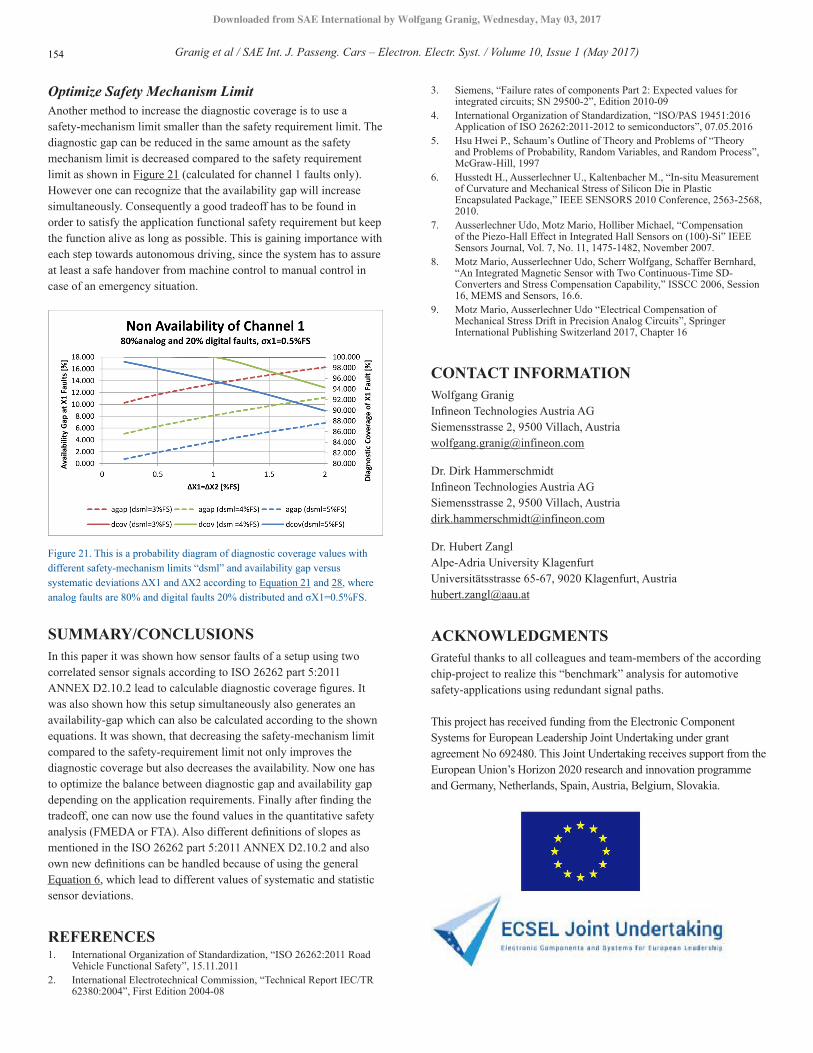
Optimize Safety Mechanism LimitAnother method to increase the diagnostic coverage is to use a safety-mechanism limit smaller than the safety requirement limit. The diagnostic gap can be reduced in the same amount as the safety mechanism limit is decreased compared to the safety requirement limit as shown in Figure 21 (calculated for channel 1 faults only). However one can recognize that the availability gap will increase simultaneously. Consequently a good tradeoff has to be found in order to satisfy the application functional safety requirement but keep the function alive as long as possible. This is gaining importance with each step towards autonomous driving, since the system has to assure at least a safe handover from machine control to manual control in case of an emergency situation.

Figure 21. This is a probability diagram of diagnostic coverage values with different safety-mechanism limits “dsml” and availability gap versus systematic deviations ΔX1 and ΔX2 according to Equation 21 and 28, where analog faults are 80% and digital faults 20% distributed and σX1=0.5%FS.

SUMMARY/CONCLUSIONSIn this paper it was shown how sensor faults of a setup using two correlated sensor signals according to ISO 26262 part 5:2011 ANNEX D2.10.2 lead to calculable diagnostic coverage figures. It was also shown how this setup simultaneously also generates an availability-gap which can also be calculated according to the shown equations. It was shown, that decreasing the safety-mechanism limit compared to the safety-requirement limit not only improves the diagnostic coverage but also decreases the availability. Now one has to optimize the balance between diagnostic gap and availability gap depending on the application requirements. Finally after finding the tradeoff, one can now use the found values in the quantitative safety analysis (FMEDA or FTA). Also different definitions of slopes as mentioned in the ISO 26262 part 5:2011 ANNEX D2.10.2 and also own new definitions can be handled because of using the general Equation 6, which lead to different values of systematic and statistic sensor deviations.

REFERENCES1. International Organization of Standardization, “ISO 26262:2011 Road

Vehicle Functional Safety”, 15.11.20112. International Electrotechnical Commission, “Technical Report IEC/TR

62380:2004”, First Edition 2004-08

3. Siemens, “Failure rates of components Part 2: Expected values for integrated circuits; SN 29500-2”, Edition 2010-09

4. International Organization of Standardization, “ISO/PAS 19451:2016 Application of ISO 26262:2011-2012 to semiconductors”, 07.05.2016

5. Hsu Hwei P., Schaum’s Outline of Theory and Problems of “Theory and Problems of Probability, Random Variables, and Random Process”, McGraw-Hill, 1997

6. Husstedt H., Ausserlechner U., Kaltenbacher M., “In-situ Measurement of Curvature and Mechanical Stress of Silicon Die in Plastic Encapsulated Package,” IEEE SENSORS 2010 Conference, 2563-2568, 2010.

7. Ausserlechner Udo, Motz Mario, Holliber Michael, “Compensation of the Piezo-Hall Effect in Integrated Hall Sensors on (100)-Si” IEEE Sensors Journal, Vol. 7, No. 11, 1475-1482, November 2007.

8. Motz Mario, Ausserlechner Udo, Scherr Wolfgang, Schaffer Bernhard, “An Integrated Magnetic Sensor with Two Continuous-Time SD-Converters and Stress Compensation Capability,” ISSCC 2006, Session 16, MEMS and Sensors, 16.6.

9. Motz Mario, Ausserlechner Udo “Electrical Compensation of Mechanical Stress Drift in Precision Analog Circuits”, Springer International Publishing Switzerland 2017, Chapter 16

CONTACT INFORMATIONWolfgang GranigInfineon Technologies Austria AGSiemensstrasse 2, 9500 Villach, [email protected]

Dr. Dirk HammerschmidtInfineon Technologies Austria AGSiemensstrasse 2, 9500 Villach, [email protected]

Dr. Hubert ZanglAlpe-Adria University KlagenfurtUniversitätsstrasse 65-67, 9020 Klagenfurt, [email protected]

ACKNOWLEDGMENTSGrateful thanks to all colleagues and team-members of the according chip-project to realize this “benchmark” analysis for automotive safety-applications using redundant signal paths.

This project has received funding from the Electronic Component Systems for European Leadership Joint Undertaking under grant agreement No 692480. This Joint Undertaking receives support from the European Union’s Horizon 2020 research and innovation programme and Germany, Netherlands, Spain, Austria, Belgium, Slovakia.



DEFINITIONS/ABBREVIATIONSASIL - Automotive Safety Integrity Level

DFA - Dependent Failure Analysis

EPS - Electric Power Steering

FMEDA - Failure Mode Effect and Diagnostic Analysis

FTA - Fault Tree Analysis

GND - Electric Ground Node

LFM - Latent Fault Metric

pdf - Probability Density Function

PMHF - Probabilistic Metric for Random Hardware Faults

SEooC - Safety Element out of Context

SPFM - Single Point Fault Metric

VDD - Electric Power Supply Node

All rights reserved. No part of this publication may be reproduced, stored in a retrieval system, or transmitted, in any form or by any means, electronic, mechanical, photocopying, recording, or otherwise, without the prior written permission of SAE International.

Positions and opinions advanced in this paper are those of the author(s) and not necessarily those of SAE International. The author is solely responsible for the content of the paper.



Documents

Calculation of Failure Detection Probability on Safety ... · RF. which are not ... We have to consider calibration inaccuracy, residual . ... described by uncertainty-offsets which