CAD of 3D Woven Nodal Textile Structures

ISSN 1746-7659, England, UK

Journal of Information and Computing ScienceVol. 4, No. 3, 2009, pp. 191-204

CAD of 3D Woven Nodal Textile Structures

Martin A. Smith + and Xiaogang Chen

School of Materials, University of Manchester, Manchester, UK

(Received February 10, 2009, accepted May 20, 2009)

Abstract. CAD of woven textile structures has received much attention in the technical textiles community. Research and development has concentrated on the simple 2D weaves and some of the 3D weaves such as angle-interlock, orthogonal, multi-layer and hollow woven structures. This paper addresses the void in the literature with respect to the more advanced and complex nodal structure and the CAD of 3D woven nodal textile structures. Innovative use of a k-ary tree data structure is used to keep track of nodal connectivity and parent-child hierarchical transformation relationships. In addition, the k-ary tree allows the design of more complex nodal configurations beyond simple ‘T’ and ‘K’ shapes due to the inherent hierarchical nature of the tree data structure. The described nodal CAD software progresses beyond the frequently encountered simple 2D interfaces of many existing textile CAD systems. 3D interfaces are used to allow the user to interactively create and edit almost any nodal configuration limited only by the weaving width of the employed loom. Novel and robust algorithms and modelling techniques are described to automate the nodal CAD process: 3D geometry specification, flattening and segmentation of nodal geometry, design paper mapping and weave architecture allocation to include: automatic computation of strut weaves, strut composite weaves and semi-automatic computation of stitching points. 3D nodal CAD has been implemented in C++ as part of the ongoing WeaveStudio CAD/CAM software system.

Keywords: CAD, textiles, woven structure, weave, nodal.

1. Introduction Two-dimensional woven fabrics are constructed from two series of yarns known as warp and weft yarns.

The warp yarns are parallel to one another and run lengthwise, whereas the weft yarns are perpendicular to the warp yarns and run crosswise. The weaving process itself results in an interlacing of warp and weft yarns to produce a woven fabric, the simplest of which is known as the plain weave as shown in Fig. 1. The graphical illustration of interlacing between warp and weft yarns is marked on design paper with each column of squares representing a warp yarn and each row of squares representing a weft yarn. A coloured square indicates that the warp yarn is lifted over the weft yarn. Conversely, a white square indicates that the warp yarn is lowered under the weft yarn. A ‘formula’ or descriptor used to describe the plain weave is 1/1. This can be interpreted as two floats in the path of the warp, i.e. one up float and one down float in the case of a plain weave. A step number can also be added to the descriptor to further describe the relative movement of a corresponding float on the next warp.

Three-dimensional woven fabrics are constructed using additional yarns that are perpendicular to both the warp and weft yarns of the aforementioned two-dimensional fabrics. Researchers have developed mathematical models for 2D and 3D weaves [1] to automate fabric construction. The mathematical models were further developed as part of a CAD package [2-4] to include the solid structures: backed, multi-layer, orthogonal and angle-interlock suitable for composites requiring thickness and delamination prevention characteristics. Further CAD development addressed hollow woven structures [5-6] based on multi-layer weaving principles and for use in applications requiring bulky, lightweight and energy absorbent composites.

+ Corresponding author. Tel.: +44-01942-274717. E-mail address: [email protected]

Published by World Academic Press, World Academic Union

Martin A. Smith, et al: CAD of 3D Woven Nodal Textile Structures 192

Fig. 1. Screenshot from WeaveStudio Nodal CAD software showing the plain weave.

A three-dimensional nodal structure consists of joining together hollow tubular struts in a variety of configurations to suit end user or application requirements and can be produced using a conventional jacquard loom. Consequently, the use of a specialised loom that is both costly and limited to specific weave architectures can be avoided. The nodal structure weave can be considered as an extension of the multi-layer weave and is a real lightweight alternative to existing bolted or welded metal components. Potential applications of nodal structures requiring both structural integrity and damage tolerance and suited to hollow tubular arrangements are wide ranging and include, for example, fully integrated bicycle frames, tennis rackets, aircraft wing ribs and walking support frames. The development of comprehensive nodal CAD/CAM software has the potential to compete with truss structures found in many diverse areas such as automotive, architectural or aerospace applications. For nodal CAD/CAM software to be considered truly comprehensive, two essential software components (in addition to CAD) are required: visualisation of tortuous yarn paths and CAM of nodal structures. Yarn path modelling and 3D visualisation including elimination of interference has been described in detail [7]. Nodal CAM with particular emphasis on choice of weave architectures relying on manual designing and the skill and experience of the technical weaver has been successfully addressed leading to the manufacture of nodal structures [8]. Design decisions leading to choice of weave architectures are not readdressed in this paper. However, algorithms are fully developed and described in this paper that facilitate CAM of nodal structures. The aim of this paper is to describe the algorithms and modelling techniques that equip the user with the tools to design and manipulate nodal structures in three-dimensional space. This aim will be achieved through the following objectives: to develop a 3D interface featuring interactive nodal creation and editing facilities; to facilitate design of complex nodal structures through the internal use of a k-ary tree data structure; to automate the flattening and segmentation of nodal geometry; to devise algorithms that discretise nodal geometry and automatically allocate weave architectures by computing weaves and composite weaves for the flattened and segmented geometry; to semi-automate the application of stitching points to bind individual weave layers together.

2. Three-Dimensional Nodal Geometry Prior to flattening and segmentation, the three-dimensional geometry of a nodal structure is specified.

The required parameters are: number of struts, planar orientation angle of a strut at the point of connectivity to another strut, dimension (length and diameter in cm) and wall thickness. The angle, length and diameter parameters are specific for each strut and it is possible to vary these parameters for each individual strut to obtain a variety of nodal configurations. The dimensions of each strut are limited by the weaving width of the employed loom. Wall thickness is discussed further in Section 5 Allocation of Weave Architectures.

A k-ary tree data structure [9] where each internal node has at most k children is used to keep track of nodal connectivity and parent-child hierarchical transformation relationships. Each internal node stores a strut’s three-dimensional geometry specification. All three-dimensional geometrical transformations in this

JIC email for contribution: [email protected]

Journal of Information and Computing Science, Vol. 4 (2009) No. 3, pp 191-204 193 section use homogenous column-major 4 matrices for strut addition, translation, rotation and reflection. All geometrical transformation operators transform strut vertices from model space to world space to position and orient a strut in relation to its parent strut. Strut deletion is achieved by detaching the deleted strut and its children from the deleted strut’s parent strut. The composite transformation matrices for the addition of a node’s strut to the k-ary tree are

4

22 rr

yr

l dTRM (1)

ppzppp

c

lMoTRoT

dTM

2

3

2

(2)

Subscripts r, p and c are used to indicate root, parent and child respectively. The root is the parent of child nodes of the root. T and R are translation and rotation matrices respectively. All rotations Ry and Rz are about the y- and z-axis respectively and all translations T are in the xy plane with the exception of Eq. (1) where the translation is in the yz plane. Mr and Mc are composite transformation matrices to position and orient the root node’s strut and child struts in the world coordinate system and in relation to its parent strut respectively. If a strut has no parent, it must be the root node in the k-ary tree. When attaching a child node’s strut to the root node’s strut Mp = Mr, otherwise Mp is the composite transformation matrix of the parent and Mp = Mc where Mc is generated from Eq. (2) for the attaching node’s parent.

The example ‘T’ nodal geometry in Fig. 2 shows the minimum three-dimensional specification for a nodal structure. The child strut in Fig. 2 (e) occupies the same space as its parent but is shown offset for illustrative purposes only. The length and diameter parameters are shown as l and d respectively and can be altered prior to transformation from model space to world space to resize individual struts according to end user or application requirements. Fig. 2 (a) also shows the world space origin, direction and up vectors for each strut as o, d and u respectively. The ‘T’ nodal consists of a horizontal parent strut (root node in the k-ary tree with the centre of the root node’s geometry defined at the origin of the world coordinate system in the xy plane) and a single attached child strut at a default orientation of 3π/2 radians to the parent measured counter-clockwise from the positive x-axis. The final applied translation matrix in Eq. (2) positions the child strut at a default distance from the parent’s origin of half a length of the parent strut in the direction of the parent strut’s direction vector. The final two applied translation matrices in Eq. (2) may appear redundant (Fig. 2 (g-i)) due to the simplicity of the ‘T’ nodal configuration, but are essential transformations for default positioning when designing more elaborate nodal structures. Fig. 2 (b) shows the model space starting position of all struts and will have an initial model space origin o = (0, 0, 0), model space direction vector d = (0, 0, 1) and model space up vector u = (0, 1, 0). Fig. 2 (d) shows the final world space position of the horizontal parent (i.e. root) strut. Fig 2 (i) shows the final world space position of the vertical child strut.

Fig. 2. Screenshots from WeaveStudio Nodal CAD software showing three-dimensional geometry specification of a ‘T’ nodal structure.

JIC email for subscription: [email protected]


are The composite transformation matrices for translation (M t), and rotation and reflection (Mr) of strut’s

MdTM pt s (3)

1, 1,1f p z z p M T o R S R T o (4a)

tzfr MpTRpTMM (4b)

In Eq. (3) if the translating strut is the root node in the k-ary tree, matrix M=Mr and the root node has no parent and therefore dp = dr. The root node’s strut is positioned independently of all descendent tree node struts. If the translating strut is not the root node, matrix M=Mc and the k-ary tree is descended and Eq. (3) is applied to translate all descendent struts. Translation in Eq. (3) uses a scalar multiple of the parent strut’s direction vector to allow interactive strut positioning using mouse selection in the CAD WeaveStudio software interface [10]. Eq. (4a) is a mirroring operation to reflect a (non-root) strut and all its descendents about the direction vector of the parent strut. Matrix S in Eq. (4a) is a scaling matrix that mirrors vertices about the x-axis. Angle α in Eq. (4a) is the angle of rotation to align dp with the x-axis. Pivot point p in Eq. (4b) is the point of rotation and is the origin of the interactively rotating strut. Angle β in Eq. (4b) is the angle

3.

attened diameter d of the two-dimensional geometry where D is the diameter of the strut prior to flattening is

of rotation about the pivot point.

Flattened and Segmented Nodal Geometry The nodal structure is transformed from three dimensions to a flattened and segmented two-dimensional

approximation with each strut assuming an oblong shape defined by four corner points. Fig. 3 shows example nodal configurations. Fig. 3 (a) is the flattened and segmented three-dimensional ‘T’ nodal structure shown in Fig. 2 with the adjoining child strut rotated from a perpendicular angle to angle β. Fig. 3 (b-e) shows examples of four additional nodal configurations with the flattened and segmented structure shown offset from the three-dimensional geometry. The nodal configurations show typical variation in strut count, dimension and orientation. Fig. 3 (f) shows the inherent hierarchical nature of the k-ary tree data structure underlying the free-form nodal geometry in Fig. 3 (e). A nodal structure is flattened after three-dimensional geometry specification and prior to two-dimensional segmentation. The approximated fl

Fig. 3. Screenshots from WeaveStudio Nodal CAD software showing a variety of nodal configurations.


Journal of Information and Computing Science, Vol. 4 (2009) No. 3, pp 191-204 195

2

Dd

(5)

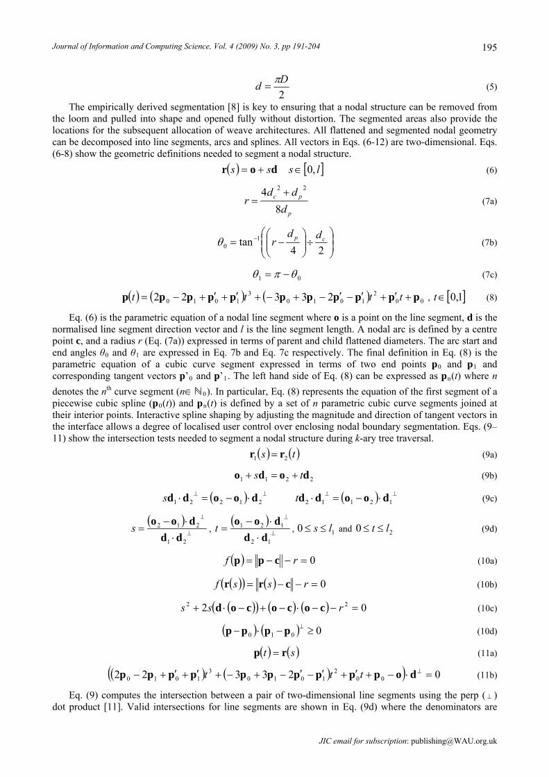
The empirically derived segmentation [8] is key to ensuring that a nodal structure can be removed from the loom and pulled into shape and opened fully without distortion. The segmented areas also provide the locations for the subsequent allocation of weave architectures. All flattened and segmented nodal geometry can be decomposed into line segments, arcs and splines. All vectors in Eqs. (6-12) are two-dimensional. Eqs. (6-8) show the geometric definitions needed to segment a nodal structure.

dor ss ls ,0 (6)

p

pc

d

ddr

8

4 22 (7a)

24tan 1

0cp dd

r (7b)

01 (7c)

002

10103

1010 23322 ppppppppppp tttt , (8) 1,0t

Eq. (6) is the parametric equation of a nodal line segment where o is a point on the line segment, d is the normalised line segment direction vector and l is the line segment length. A nodal arc is defined by a centre point c, and a radius r (Eq. (7a)) expressed in terms of parent and child flattened diameters. The arc start and end angles θ0 and θ1 are expressed in Eq. 7b and Eq. 7c respectively. The final definition in Eq. (8) is the parametric equation of a cubic curve segment expressed in terms of two end points p0 and p1 and corresponding tangent vectors p’0 and p’1. The left hand side of Eq. (8) can be expressed as pn(t) where n

denotes the nth curve segment (nℕ0). In particular, Eq. (8) represents the equation of the first segment of a piecewise cubic spline (p0(t)) and pn(t) is defined by a set of n parametric cubic curve segments joined at their interior points. Interactive spline shaping by adjusting the magnitude and direction of tangent vectors in the interface allows a degree of localised user control over enclosing nodal boundary segmentation. Eqs. (9–11) show the intersection tests needed to segment a nodal structure during k-ary tree traversal.

ts 21 rr (9a)

2211 dodo ts (9b)

21221 doodds 12112 dooddt (9c)

21

212

dd

doos ,

12

121

dd

doot , 10 ls and 20 lt (9d)

0 rf cpp (10a)

0 rssf crr (10b)

02 22 rss cococod (10c)

0010 pppp (10d)

st rp (11a)

023322 002

10103

1010 dopppppppppp ttt (11b)

Eq. (9) computes the intersection between a pair of two-dimensional line segments using the perp ( ) dot product [11]. Valid intersections for line segments are shown in Eq. (9d) where the denominators are


Martin A. Smith, et al: CAD of 3D Woven Nodal Textile Structures 196 non-zero and l1 and l2 are line segment lengths. Eq. (10) computes the intersection between an arc and line segment. Eq. (10a) is the implicit equation of a circle where p is any point on the circle’s circumference, c is the centre point and r is the radius. Eq. (6) is substituted into Eq. (10a) to obtain Eqs. (10b-10c) resulting in a quadratic equation in s. When s is substituted into Eq. (6) up to two intersection points are generated. The points are tested further for arc intersection using Eq. (10d) where p is the point to be tested and p0 and p1 are the arc end points corresponding to θ0 and θ1 in Eq. 7b and Eq. 7c respectively. Eq. (11) computes the intersection between a spline and a line segment and the roots of the equation can be obtained by a numerical method such as interval bisection [12].

4. Discretisation: Mapping from 2D Geometry to Design Paper A key technical challenge in preparation for nodal manufacture is to map the two-dimensional flattened

and segmented geometry to design paper representation. The discretisation algorithm is essential to allow subsequent user allocation of weave architectures and layer integration through yarn editing and stitching. The mapping determines the number of design paper rows and columns for a given strut by scaling the four corner points of a strut’s oblong

,warp weft v S v (12)

The homogenous column-major matrix S in Eq. (12) is a scaling matrix that scales a box corner point v by factors warp, weft i.e. the user specified nodal warp yarns per cm and weft yarns per cm respectively.

33

Fig.4 shows an example discretisation of a ‘T’ nodal structure.

Fig. 4. Screenshots from WeaveStudio Nodal CAD software showing discretisation of a ‘T’ nodal structure.

Fig. 4 (a) shows the design paper with discretised segments using sets of connected triangles that, compared with other polygons, allow any surface to be tessellated. Fig. 4 (b) shows the same discretised segments separated to clearly indicate each distinct triangle set for each constituent segment. All concave segmented areas are partitioned into convex regions to allow each region to be tessellated into a single triangle fan. An example tessellation is shown in Fig. 4 (c) for one of the two convex regions of segment 10. A triangle fan of n vertices is defined as an ordered vertex list (v0, v1, …,vn-1) and where the ith triangle (0 ≤ i



< n – 2) Ti is defined as v0, v i+1, vi+2.

In order to identify correct individual warp and weft coordinate locations on the design paper, a mapping algorithm is needed to convert the real number triangular geometric description to a discrete natural number design paper representation. A design paper square, design paper row and design paper column are subsequently referred to as square, row and column respectively. The mapping algorithm has to map to warp and weft coordinate locations in such a manner as to guarantee that square generation is not omitted or duplicated resulting in incorrect weave interlacement on the design paper. A square that is within the boundary of a triangle is a valid warp/weft coordinate, but special care needs to be exercised for those square centres that lie exactly on a triangle boundary. Fig. 5 (a) shows two triangles overlaid on a subset of the discrete design paper and abut against a common edge. If two triangles abut against a common edge, only one triangle results in production of the squares along the common edge during the mapping algorithm. A top-left fill convention can be defined that prevents duplicate square production in cases where triangles in a fan share a common edge. The convention considers a square inside the boundary of a triangle if either of four conditions are met for the square’s centre: it is on or to the right of a left edge, strictly to the left of a right edge, on or below the top edge or strictly above the bottom edge. Mapping must be performed in a consistent manner using this fill convention to prevent overlaps and gaps during square generation.

Fig. 5. Top-left fill convention to identify correct individual warp and weft coordinate locations.

The triangle in Fig. 5 (b) shows left edges with dark solid line segments and a right edge with a light dashed line segment. The triangle in Fig. 5 (b) has neither a top nor bottom edge. Assuming a counter clockwise ordering of a triangle’s vertices, a downward pointing arrow indicates a left edge and an upward pointing arrow indicates a right edge. The mapping algorithm calculates edge deltas and inverse gradients in counter clockwise order 30 i using modular arithmetic.

1 mod3i iiy y y (13a)

1 mod3i iix x x (13b)

1 ii

i

xm

y

(13c)

Edge identification is for a left edge, 0y 0y for a right edge, 0y and for a bottom

edge and and for a top edge. The common edge on the design paper in Fig. 5 (a) is the left edge of the upper-right triangle and the right edge of the lower-left triangle. The upper-right triangle also has a top and a right edge. The lower-left triangle also has a bottom and a left edge. It can be seen from Fig. 5 (a) that the triangle on the design paper with vertices v

0x0y 0x

0 = (1, 6), v1 = (6, 1) and v2 = (6, 6) produces 15 (dark) squares. The triangle on the design paper with vertices v0 = (1, 6), v1 = (1, 1) and v2 = (6, 1) produces 10 (grey) squares. Because the shared edge is a left edge of the upper-right triangle, that triangle produces the



y

squares along the shared edge. Table 1 summarises the squares generated using the top-left fill convention as applied to the example triangle boundaries in Fig. 5 (a).

The mapping algorithm computes the inverse gradient in Eq. (13c) for each of the triangle edges and is used to calculate the change in x per unit change in y for each row. The algorithm produces squares in horizontal spans a row at a time as a triangle is traversed from top to bottom and from left to right. The

starting and ending row values (where ystart, end ℕ1 and y i, yj ℝ) that adhere to the top-left fill convention are

istart yy (14)

1 jend yy (15)

Table 1. Summary of top-left fill convention rules applied to triangle boundaries in Fig. 5 (a).

Edge Boundary Rule (i.e. square

centres with respect to the edge) Squares Generated

Lower-left triangle: left edge On or to the right of the left edge Yes

Lower-left triangle: bottom edge Above the bottom edge No

Lower-left triangle: right edge To the left of the right edge No

Upper-right triangle: right edge To the left of the right edge No

Upper-right triangle: top edge On or below the top edge Yes

Upper-right triangle: left edge On or to the right of the left edge Yes

For Eqs (14-15) yi > yj and are the y coordinates of a triangle edge. The C/C++ floor function (⌊⌋) [13] is defined as returning the largest integer that is less than or equal to its argument. The starting row for the top of a triangle starts at the topmost y-coordinate that lies within the interior of the triangle or y0 if y0

happens to lie exactly on a natural number boundary. Fig. 6 (a) shows example triangles with the floor function from Eqs. (14-15) applied to obtain the correct starting (ystart) and ending (yend) row values. The left of Fig. 6 (a) shows a flat top triangle. From top to bottom counter clockwise it has a top, left and right edge respectively. The right of Fig. 6 (a) shows a flat bottom triangle. From top to bottom counter clockwise it has a left, bottom and right edge respectively.

The small differential change resulting from Eq. (14) needs to be accounted for when calculating the starting and ending column values for the first row.

01

00 yymxx startleft (16)

01

20 yymxx startright (17)

startx (18) leftx

Fig. 6. Mapping from continuous to discrete starting and ending row and starting column values.



endx - 1 (19) rightx

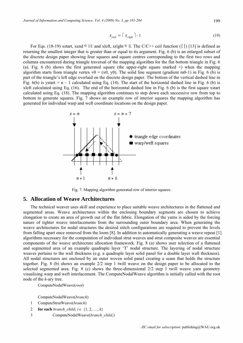
For Eqs. (18-19) xstart, xend ℕ1 and xleft, xright ℝ. The C/C++ ceil function (⌈⌉) [13] is defined as returning the smallest integer that is greater than or equal to its argument. Fig. 6 (b) is an enlarged subset of the discrete design paper showing four squares and square centres corresponding to the first two rows and columns encountered during triangle traversal of the mapping algorithm for the flat bottom triangle in Fig. 6 (a). Fig. 6 (b) shows the first generated square (the upper-right square marked +) when the mapping algorithm starts from triangle vertex v0 = (x0, y0). The solid line segment (gradient m0-1) in Fig. 6 (b) is part of the triangle’s left edge overlaid on the discrete design paper. The bottom of the vertical dashed line in Fig. 6(b) is ystart = n – 1 calculated using Eq. (14). The start of the horizontal dashed line in Fig. 6 (b) is xleft calculated using Eq. (16). The end of the horizontal dashed line in Fig. 6 (b) is the first square xstart calculated using Eq. (18). The mapping algorithm continues to step down each successive row from top to bottom to generate squares. Fig. 7 shows an example row of interior squares the mapping algorithm has generated for individual warp and weft coordinate locations on the design paper.

Fig. 7. Mapping algorithm generated row of interior squares.

5. Allocation of Weave Architectures The technical weaver uses skill and experience to place suitable weave architectures in the flattened and

segmented areas. Weave architectures within the enclosing boundary segments are chosen to achieve elongation to create an area of growth out of the flat fabric. Elongation of the yarns is aided by the forcing nature of tighter weave interlacements from the surrounding outer boundary area. When generating the weave architectures for nodal structures the desired stitch configurations are required to prevent the levels from falling apart once removed from the loom [8]. In addition to automatically generating a weave repeat [1] algorithms necessary for the computation of individual strut weaves and strut composite weaves are essential components of the weave architecture allocation framework. Fig. 8 (a) shows user selection of a flattened and segmented area of an example quadruple layer ‘T’ nodal structure. The layering of nodal structure weaves pertains to the wall thickness (e.g. a quadruple layer solid panel for a double layer wall thickness). All nodal structures are enclosed by an outer woven solid panel creating a seam that holds the structure together. Fig. 8 (b) shows an example 2/2 step 1 twill weave on the design paper to be allocated to the selected segmented area. Fig. 8 (c) shows the three-dimensional 2/2 step 1 twill weave yarn geometry visualising warp and weft interlacement. The ComputeNodalWeave algorithm is initially called with the root node of the k-ary tree.

ComputeNodalWeave(root)

ComputeNodalWeave(branch)

1 ComputeStrutWeave(branch)

2 for each branch_childi i {1, 2, …, k}

3 ComputeNodalWeave(branch_childi)



Line 1 of ComputeNodalWeave calls ComputeStrutWeave for a given branch (initially the root) of the k-ary tree. Lines 2-3 iterate over the remaining child nodes of the given branch to recursively compute the remaining nodal weave for the entire nodal structure. It should be noted that the use of an underscore in the pseudocode denotes access to data structure attributes (e.g. branch_childi or branch_segmenti accesses the ith child or segment respectively of a branch of the k-ary tree). The ComputeStrutWeave algorithm is called with a given branch of the k-ary tree.

ComputeStrutWeave(branch)

1 for each branch_segmenti i {1, 2, …, m}

2 weaveorigin = ComputeWeaveOrigin(branch_segmenti)

3 for each segmenti_squarej j {1, 2, .., n}

4 repeatrow = ((squarej_row – weaveorigin_row) mod weaverows) + 1

5 if (repeatrow < 1)

6 repeatrow += weaverows

7 repeatcolumn = ((squarej_column – weaveorigin_column) mod weavecolumns) + 1

8 if (repeatcolumn < 1)

9 repeatcolumn += weavecolumns

10 segmentweave = weaverepeat_column square_row, squareted,layerselec jjrepeatrow, repeatcolumn

Line 1 iterates over each flattened and segmented area of the given branch in order to compute the weave for the entire strut. Line 2 computes the segment’s weave origin (weaveorigin) that is initialised to the lower-left corner of the axis-aligned bounding rectangle of the segment allocated weave. Fig. 8 (d) shows the weave origin as a cross that can be interactively selected and moved within the bounding rectangle to reposition the weave within the segmented area. Fig. 8 (d) also shows the design paper for layer one of a quadruple layer segment. The squares for a 2/2 step 1 twill weave can be identified within the bounding rectangle’s segmented area. All other remaining dark squares indicate a subset of the interior regions of the ‘T’ nodal yet to be allocated weaves. All other remaining white squares indicate a subset of the exterior region of the ‘T’ nodal (i.e. the solid panel) that is also yet to be allocated a weave. Line 3 iterates over each design paper square of the given flattened and segmented discretised area (described in Section 4 Discretisation: Mapping from 2D Geometry to Design Paper) to begin weave allocation for that segment. Lines 4-9 compute the row and column indices (repeatrow and repeatcolumn) of the weave repeat (weaverepeat) using modular arithmetic. The number of weaverows and weavecolumns are the number of weave rows and columns for the weave repeat respectively. In the example twill weave in Fig. 8 (b) there are four weave rows and four weave columns. Line 10 indexes into the weave repeat to perform a lookup from weaverepeat and assignment to the active layer layerselected (e.g. layer one in Fig. 8 (a-d)) of the segment’s weave (segmentweave). The weaverepeat and segmentweave data structures are implemented as 2D and 3D arrays respectively as can be seen by the subscript indexing in line 10 and schematic in Fig. 8 (e). Line 10 effectively tiles the weave repeat (i.e. unit weave) across the segmented area starting at the weave origin. Fig. 8 (b) shows an example 2/2 twill weave repeat and corresponding tiled segmented area in Fig. 8 (d). All indexing in the pseudocode (e.g. layer, row, column etc) starts at one. Access to array elements for segmentweave are by layer, square row and square column respectively. The kth layer selected (layerselected) k {1, 2, .., p} is user selected in the CAD nodal weave yarn editor interface.

The mechanics of k-ary tree traversal for ComputeNodalCompositeWeave are identical to ComputeNodalWeave and are not repeated here.

ComputeNodalCompositeWeave(root)

ComputeNodalCompositeWeave(branch)

1 ComputeStrutCompositeWeave(branch)

2 for each branch_childi i {1, 2, …, k}

3 ComputeNodalCompositeWeave (branch_childi)

ComputeStrutCompositeWeave(branch)

1 for each branch_segmenti i {1, 2, …, m}



2 for each segmenti_squarej j {1, 2, .., n}

3 for each layerk k {1, 2, .., p}

4 row = layerk + (squarej_row – 1) layers

5 column = layerk + (squarej_column – 1) layers

6 designpaperrow, column = segmentweave _column square_row, square,layer jjk

7 for each rowl l {1, 2, .., layers - layerk}

8 designpaper = LIFTER column ,rowrow l

Lines 1-3 of ComputeStrutCompositeWeave iterate over each segment, square and layer respectively of the given branch in order to compute the composite weave for the entire strut. Lines 4-5 compute the row and column indices (row and column) to index into the design paper (designpaper) in line 6 and line 8. layers in lines 4-5 are the total number of layers for the nodal structure (e.g. four layers in Fig. 8). segmentweave in line 6 is computed in line 10 of ComputeStrutWeave. Fig. 8 (f) shows the design paper for an example composite weave for a quadruple layer segment of a ‘T’ nodal structure. All segment layers have been allocated a simple 2/2 twill step 1 weave in the example for the purpose of illustration. Lines 7-8 iterate over specified rows (rowl) to assign the LIFTER instruction to instruct the loom to lift the warp yarns over the weft yarns for the computed coordinate locations on the design paper. The LIFTER notation is shown as ‘\’ in Fig. 8 (f) and means a warp yarn is lifted when a weft yarn from a lower layer is to be inserted.

As an example, consider the square region of design paper in Fig. 8 (f) where the two pairs of parallel lines intersect. In the first column, proceeding from bottom to top the notation is ‘ \\\’. The corresponding yarn interlacement can be seen in Fig. 8 (g) by considering layer 1, warp yarn 105, and weft yarns 241-244. The notation ‘ ’ indicates layer 1 warp yarn 105 passes over layer 1 weft yarn 241. The LIFTER notation ‘\\\’ indicates layer 1 warp yarn 105 passes over weft yarns 242-244 corresponding to layers 2-4 respectively.

The ComputeStitchingPoints algorithm is critical and allows the user to interactively edit yarn interlacement to stitch together individual layers transforming them into attached multi-layer weaves. The ComputeStitchingPoints algorithm drives the logic to perform design paper lookup and updates to accurately show correct yarn interlacement and stitching points.

ComputeStitchingPoints()

1 rowstart = weftSelected – ((weftSelected – 1) mod layers)

2 warpbits = (1 << layers) - 1

3 for each rowi i {rowstart, rowstart + 1, …, rowstart + layers - 1}

4 if (designpaper = WARPDOWN) column ,rowi

5 exit for each

6 if (designpaper = WARPDOWNSTITCH) column ,rowi

7 exit for each

8 warpbits >>= 1

9 if (warpbits = 0) warpbits = (1 << layers) – 1 else warpbits >>= 1

10 warpmask = 1 << (layers – 1)

11 for each rowi i {rowstart, rowstart + 1, …, rowstart + layers - 1}, layerj j {1, 2, …, layers}

12 if (layerj > layerselected)

13 if (warpbits & warpmask) designpaper = LIFTER column ,rowi

14 else designpaper = WARPSTITCHDOWN column ,rowi

15 else if (layerj = layerselected)

16 if (warpbits & warpmask) designpaper = WARPUP column ,rowi

17 else designpaper = WARPDOWN column ,rowi

18 else if (layerj < layerselected)



19 if (warpbits & warpmask) designpaper = WARPSTITCHUP column ,rowi

20 else designpaper = WARPDOWN column ,rowi

21 warpmask >>= 1

Lines 1-9 of ComputeStitchingPoints include iteration over specified rows (rowi) to perform design paper lookup to compute the bit set warpbits. For the quadruple layer example shown in Fig. 8 warpbits post loop can compute to 11112, 1112, 112, 12 or 02 depending on one of five possible positions of interlacement/stitching points as the user cycles through the interlacement/stitching possibilities for a given warp yarn. As an example and referring to Fig. 8 (g) and given a user selection of weft yarn 243 using the mouse, weftselected = 243, layers = 4 for a quadruple layer weave, rowstart = 241, warpbits = 11112 pre loop, rowi {241, 242, 243, 244}, column = 107 (107th warp yarn pertaining to layer 3 as a result of user selection of weft yarn 243), warpbits = 12 post loop where all values are in base 10 unless explicitly stated to be in base 2 using the 2 subscript. As the user repeatedly selects weft yarn 243 in the yarn editor interface, the stitching points and interlacement notation for warp yarn 107, layer 3 are cycled repeatedly in the following sequence: ‘ \’ ‘ \’ ‘ ’ ‘ \’ ‘ \’.

In the example in Fig. 8 (f-g) the user has cycled the interlacement/stitching points from the default 2/2 twill four layer interlacement ‘ \’ to ‘ \’ where ‘ ’ denotes warp stitch down and ‘ ’ denotes warp stitch up. Consider the square region of design paper in Fig. 8 (f) where the two pairs of parallel lines intersect and weft yarns 241-244 in Fig. 8 (g). It can be seen from the design paper and yarn editor that warp yarn 107, layer 3 stitches up to layer 2. It can also be seen that warp yarn 106, layer 2 stitches down to layer 3. Lines 10-21 include iteration over specified rows (rowi) and layer numbers (layerj). Comparisons between the layer number (layerj) and the user selected layer number (layerselected) in addition to application of the C/C++ bitwise & operator [13] between warpbits bit set and warpmask bit mask drive design paper update of interlacement and stitching notation. Eq. (8) is used to compute a set of piecewise cubic splines for each yarn path in the nodal weave yarn editor shown in Fig. 8 (g).

6. Conclusions The CAD of 3D woven nodal textile structures has been implemented in the C++ programming language

as part of the bespoke WeaveStudio CAD/CAM software tool [10]. Simple 2D interfaces were previously employed to specify CAD of 3D woven structures such as multi-layer, orthogonal and angle-interlock weaves. However, the more advanced and complex nodal weaves necessitate intuitive, interactive and user-friendly 3D interfaces for nodal structure creation and manipulation as shown in Fig. 2 and Fig. 3. All stages of nodal structure design have been fully automated through the development of the nodal CAD software with the exception of the nodal weave yarn editor tool. The k-ary tree data structure permits users to hierarchically create, attach and edit individual struts to compose a variety of nodal configurations. The 3D geometry is approximated by flattened and segmented regions and automatically mapped to design paper representation in preparation for weaving. Weaves can be automatically allocated to individual flattened and segmented regions. Once the technical weaver has chosen suitable weaves, composite weaves are automatically computed for multi-layer nodal structures. The nodal weave yarn editor tool is semi-automated out of necessity as the skill and experience of the technical weaver is needed when applying stitching points and editing individual yarn paths to tailor and customise allocated weaves. However, the design paper is automatically updated with stitching points and warp and weft yarn interlacement resulting from yarn editor manipulations. The design paper representation (e.g. Fig. 8 (f)) can be used as the basis for lifting plans that instruct the loom to manufacture nodal structures.



Fig. 8. Screenshots (a-d, f-g) from WeaveStudio Nodal CAD software and schematic (e) all showing key stages of weave architecture allocation.

7. References

[1] X. Chen, R.T. Knox, D.F. McKenna, R.R. Mather. Automatic generation of weaves for the CAM of 2D and 3D

woven textile structures. J.Text. Inst.. 1996, 87: 356-370.

[2] X. Chen, P. Potiyaraj. CAD/CAM for complex woven fabrics part I: backed cloths. J.Text. Inst.. 1998, 89: 532-370.

[3] X. Chen, P. Potiyaraj. CAD/CAM for complex woven fabrics part II: multi-layer fabrics. J.Text. Inst.. 1999, 90: 73-

90.

[4] X. Chen, P. Potiyaraj. CAD/CAM of orthogonal and angle-interlock woven structures for industrial applications.

Text. Res. J.. 1999, 69: 648-655.

[5] X. Chen, Y.L. Ma, H.Zhang. CAD/CAM for cellular woven structures. J.Text. Ins.t. 2004, 95: 229-241.


Martin A. Smith, et al: CAD of 3D Woven Nodal Textile Structures


204

[6] X. Chen, H. Wang. Modelling and computer-aided design of 3D hollow woven reinforcement for composites.

J.Text. Inst.. 2006, 97: 79- 87.

[7] M.A. Smith, X.Chen. CAD and constraint-based geometric modelling algorithms for 2D and 3D woven textile

structures. J. Information and Computing Science. 2008, 3(3): 199-214.

[8] L.T. Taylor. Design and manufacture of 3D nodal structures for advanced textile composites, PhD thesis.

University of Manchester, UK, 2002-2007.

[9] T.H. Cormen, C.E. Leiserson, R.Rivest. Introduction to Algorithms. Cambridge: MIT Press Inc., Massachusetts,

1990.

[10] M. Smith, X.Chen. WeaveStudio CAD/CAM software for 3D woven structures. EPSRC funded project, University

of Manchester, UK, 2005-2008.

[11] F.S. Hill Jr. The pleasures of ‘perp dot’ products. Graphics Gems IV. Academic Press, 1994.

[12] R.W. Hamming. Numerical Methods for Scientists and Engineers, 2nd Ed.. Dover Publishing Inc., 1987.

[13] B. Stroustrup. The C++ Programming Language, 3rd Ed.. Addison Wesley Longman, Reading MA., 1997.

Documents

CAD of 3D Woven Nodal Textile Structures