c?..-l 11 l - NASA...Price N.A. I hincZ IS, z I w t m J m I = _ 7--w w PREPARATION OF THE REPORT DOCUMENTATION PAGE The last page of a report facing the third cover is the Report Documentation

c?..- l_11_ l

ANALYSIS k:_ SPALL LIFE

IN 440C-m_L BEARING RIMS

.... _ __::_i ...........

https://ntrs.nasa.gov/search.jsp?R=19910012213 2020-04-25T05:40:18+00:00Z

....... w

u

_m_

ImJ ..... "....

__ _Nmr .....

m

m

m --_=_--z-- _ : :

AFFILIATIONS

i)

2)

3)

4)

5)

P.C. Bastias, J. Du, V. Gupta, G.T. Hahn, X. Leng, and C. A.

Rubin are with Vanderbilt University, Nashville, TN.

A.P. Bower is with Cambridge University, U.K.

V. Bhargava is with General Electric Corporate Research

Laboratory, Schenectady, N.Y.

S.M. Kulkarni is with TRW Safety Systems/Mesa, Mesa, AZ.

A.M. Kumar is with Washington State University, Pullman, WA.

! - .

w

.

,

,

•

TABLE OF CONTENTS

paqe

ABSTRACT ............................................. iii

LIST OF FIGURES ...................................... iv

LIST OF TABLES ....................................... xxii

INTRODUCTION ......................................... 1

i.i Background ...................................... 1

1.2 Summary ......................................... 2

CYCLIC STRESS-STRAIN PROPERTIES ...................... 5

2.1 Background ...................................... 5

2.2 Experimental Procedures ......................... 9

2.3 Cyclic Stress-Strain Properties of 440C Steel...ll

2.4 Cyclic stress-Strain Properties of 7075-T6

Aluminum ........................................ 17

2.5 Discussion and Conclusions ...................... 17

FINITE ELEMENT ANALYSES .............................. 28

3.1

3.2

3.3

3.4

3.5

3.6

Background ...................................... 28

Analytical Procedures ........................... 31

Three-Dimensional Rolling Contact of

Bearing Steel ................................... 40

Three-Dimensional Rolling Contact of

Hardened Aluminum ............................... 67

Two-Dimensional Rolling-Plus-Sliding with

Heat Generation ................................. 82

Conclusions ..................................... 94

EVALUATION OF THE FRACTURE MECHANICS DRIVING FORCE

FOR SPALL GROWTH ..................................... 96

4.1

4.2

4.3

4.4

4.5

4.6

Background ...................................... 96

Contributions to the Spall Growth Driving

Force, .......................................... 96

Evaluation of the Mode I and Mode II Driving

Force for Two-Dimensional, Surface Breaking

Cracks with Fluid in the Crack Cavity ........... 99

Comparisons of the Contributions to the

Driving Force for Surface Breaking Cracks ....... i01Evaluation of the Threshold Crack Sizes ......... 133

Conclusions ..................................... 137

ROLLING CONTACT FAILURE .............................. 138

5.1

5.2

Background ...................................... 138

Experimental Materials and Procedures ........... 138

g

i

m

l

qm

i

mm

m

u

t

,

5.3

5.4

5.5

5.6

5.7

5.8

GENERAL DISCUSSION ...................................

Retained Austenite .............................. 171

Nucleation Vs. Growth ........................... 171

Surface Roughness ............................... 181

Replication and Metallographic Studies of

Spalls in 440C Steel ............................ 181

Rolling Contact of Hardened Aluminum ............ 185Conclusions ..................................... 186

188

6.1

6.2

6.3

6.4

Finite Element Calculations of Contact

Plasticity ...................................... 188

Spall Nucleation ................................ 189

Growth and Spalling ............................. 190Conclusions ..................................... 191

7. CONCLUSIONS .......................................... 196

8. ACKNOWLEDGEMENTS ..................................... 199

REFERENCES ................................................ 200

APPENDIX I. 3-DIMENSIONAL DISPLACEMENT BOUNDARY

CONDITIONS ................................. 210

APPENDIX 2. BOUNDARY CONDITIONS FOR 2-DIMENSIONAL

ROLLING-PLUS-SLIDING CONTACT WITH

FRICTIONAL HEATING ......................... 218

APPENDIX 3. STRESS-STRAIN CONTOURS FOR 3-

DIMENSIONAL ROLLING CONTACT OF HARDENED

ALUMINUM ................................... 230

w

w

= :

LI:J o

Report Documentation Page

1. Report No. 2. Government Accession No.

4. Tide and Subtitle

ANALYSIS OF ROLLING CONTACT SPALL LIFE IN 440C

BEARING RIMS FINAL REPORT

7. Author(s)

Pedro C. Bastias, Vivek Bhargava, Allan P. Bower,

Jianqun Du, Vikas Gupta, George T. Hahn, Sanjeev M.

Kulkarni, Arun M. Kumar, Xiaogang Leng, and Carol A.Rubin

9. Performing Organization Name and Addre_' '

Vanderbilt University,

Center for Materials TribologyP.O. Box 1S93 - Station B

Na_hvi11P TN 37_3_12. Spon_ring A_ency Name and Address

National Aeronautics and Space Administration

Harshall Space Flight Center

Huntsville, AL 35812

3. Recipient's Catalog No.

5. Report Date

Januar_ 23, 19916. Performing Organizat/on Code

None

8. Performing Organization Report No,

10. Work Unit No.

11. Contract or Grant No.

NAS8-37764

13. Type of Report and Period Covered

Final Report

14. Sponsoring Agency Code

15. SupDlementary Notes

Project Monitor, Steve Gentz, NASA Marshall Space Flight Center

_. Abstract

This report describes the results of a 2-year study of the mechanism of spall

failure in the HPOTP bearings. The objective was to build a foundation for

detailed analyses of the contact life in terms of: (i) cyclic plasticity, (ii)

contact mechanics, (iii) spall nucleation and (iv) spall growth. Since the

laboratory rolling contact testing is carried out in the 3-ball/rod contact fatigue

testing machine, the analysis of the contacts and contact lives produced in this ma,

received attention. The results from the experimentally observed growth lives are

compared with calculated predictions derived from the fracture mechanics ealculatio

t7. Key Words (Suggested by Author(s))

Spalling; Fatigue; Failure Mechanisms;

Stress Intensity Factors; HPOTP Bearings

18. Distribution Statement

Unclassified - Unlimited

19 Security Ctassif, _of th_s repoc_

Unclassified

* 20. Security Classd (of this paget

: Unclassified

21 No of pages

249I 22. Price

N.A.

I

hincZ

IS,

z

I

wt

m

J

m

I

= _

7--

w

w

PREPARATION OF THE REPORT DOCUMENTATION PAGE

The last page of a report facing the third cover is the Report Documentation Page, RDP. Information presented on thispage is used in announcing and cataloging reports as well as preparing the cover and title page. Thus it is important

that the information be correct. Instructions for filling in each block of the form are as follows:

Block 1. Report No. NASA report series number, ifpreassigned.

Block 2. Government Accession No. Leave blank,

Block 3..Recipient's Catalog No. Reserved for use by eachreport recipient.

Block 4. Title and Subtitle. Typed in caps and lower casewith dash or period separating subtitle from title.

Block 5. Report Date. Approximate month and year the

report will be published.

Block 6, Pe.rformincj Organization Code. Leave blank.

Block 7. Author(s). Provide full names exactly as they are

to appear on the title page. tf applicable, the word editorshould follow a name.

Block 8. Performing Organization Report No. NASA in-stallation report control number and, if desired, the non-NASA performing organization report control number.

Block 9. Performing Organization Name and Address. Pro-vide affiliation (NASA program office, NASA installation,or contractor _ame) of authors.

Block 10. Work Unit No. Provide Research and

Technology Objectives and Plans (RTOP) number.

Block 11. Contract or Grant No. Provide when applicable.

Block 12. Sponsoring Ac_enc¥ Name and Address.National Aeronautics and S_ace Administration, Washing-ton, D.C. 20546-0001. If contractor report, add NASA in-stallation or HQ program office.

BI_:_ 13. Type of Report and Period Covered. NASA for-mal report series; for Contractor Report also list type (in-terim, final) and period covered when applicable.

Block 14. Sponsorinc J Agenc¥ Code. Leave blank.

Block 15. Supplementary Notes. Information not includedelsewhere_affiliation of authors if additional space is re-

quired for block 9, notice of work sponsored by anotheragency, monitor of contract, information about sup-plements (film, data tapes, etc.), meeting site and date forpresented papers, journal to which an article has been sub-mitred, note of a report made from a thesis, appendix byauthor other than shown in block 7.

Block 16. Abstract. The abstract should be informative

rather than descriptive and should state the objectives ofthe investigation, the methods employed (e.g., simulation,experiment, or remote sensing), the results obtained, andthe conclusions reached.

Block 17. Key Words. Identifying words or phrases to beused in cataloging the report.

Block 18. Distribution Statement. Indicate whether reportis available to public or not. If not to be controlled, use"Unclassified-Unlimited." If controlled availability is re-quired, list the category approved on the DocumentAvailability Authorization Form (see NHB 2200.2, Form

FF427). Also specify subject category (see "Table of Con-

tents" in a current issue of STA._._R),in which report is tobe distributed.

Block 19. Security Classification (of this report).Self-explanatory.

Block 20. Security Classification (of this page).Self-explanatory.

Block 21, No. of pages. Count front matter pages begin-ning with iii, text pages including internal blank pages, andthe RDP, but not the title page or the back of the title page.

Block 22. Price Code. If block 18 shows "Unclassified-

Unlimited," provide the NTIS price code (see "NTIS PriceSchedules" in a current issue of STAR) and at the bot-tom of the form add either "For sale by the NationalTechnical Information Service, Springfield, VA22161-2171" or "For sale by the Superintenderrt ofDocuments, U.S. Government Printing Office,Washington, DC 20402-0001," whichever is appropriate.

ABSTRACT

This report describes the results of a 2-year study of the

mechanism of spall failure in the HPOTP bearings. The objective

was build a foundation for detailed analyses of the contact life

in terms of; (i) cyclic plasticity, (ii) contact mechanics, (iii)

spall nucleation and (iv) spall growth. Since the laboratory

rolling contact testing ......carried out in the 3-ball-rod contact

fatigue testing machine, the analysiss of the contacts and

contact lives produced in this machine received attention.

The analysis of previous cyclic stress-strain hysteresis

loop measurements of 440C steel was refined to account for the

plasticity of the fillet regions. In addition, the hysteresis

loop shapess of the hardened 7075 aluminum alloy were measured.

In both cases the elastic-linear-kinematic-hardening-plastic

(ELKP) loop parameters were evaluated. Elasto-plastic, finite

element analyses of the repeated, 3-dimensional, frictionless,

rolling contact produced in the 3-ball-rod testing machine at

Hertzian pressures of Po = 2.4, 4.0 and 5.4 GPa (for 440C steel)

and 1.25 GPa (for hardened aluminum) were carried out using the

appropriate ELKP-loop parameters. These calculations were also

extended for 440C steel properties to 3-dimensional rolling-plus-

sliding and to the 2-dimensional (line contact) thermal-

mechanical coupled rolling-plus-sliding with frictional heating.

The results of calculations are compared with observations of

aluminum rods subjected to contact under these conditions.

Rolling contact tests of the 440C steel and the hardened

aluminum were performed in the 3-ball-rod testing machine with

smooth and roughened balls. Efforts were made to evaluate the

effects of retained austenite. A series of tests were performed

on the 440C samples with small = i00 _m indentations in the

running track which make it possible to locate and follow the

progress of spall nucleation and growth. The results define the

spall nucleation- and spall growth-component of the contact life

of the 440C steel over a range of the contact pressures. They

also provide evidence for a threshold pressure for crack growth.

In addition, the 3-dimensional features of the spall were studied

by a novel replicating technique and metallographic sections of

the spalls.

The contributions to the fracture mechanics crack growth

driving force for surface breaking cracks arising from the

Hertzian stresses, surface irregularities, fluid in the crack

cavity, centrifugal stresses and thermal stresses are reviewed

and the results of 2- and 3-dimensional analyses are compiled and

compared. New calculations for the Bower model of a 2-dimensional

surface breaking crack with fluid pressure in the crack cavity

are pressented. A numerical expression for the Mode I crack

driving force for a 3-dimensional crack with fluid in the crack

cavity is used to calculate the spall growth component of the

contact life. These calculations are compared with and are in

reasonable agreement with the measurements of spall growth.

iii

i

ms

U

mu

m

U

w

I

J

m

i

m

w

mm

m

w

z

w

w

m

= =

r

w

Fiqure

2.1

2.2

2.3

2.4

2.5

2.6

2.7

LIST OF FIGURES

Shear stress-shear strain hysteresis loops:

(a) the loop for idealized, isotropic,

elastic-perfectly-plastic (EPP) behavior,

and (b) the loops displayed by 440C steel

after N=I5 and N=250 stress cycles. While

the EPP-loop is drawn so that its 0.035%-

offset, shear yield strength corresponds with

that of the N=I5 loop of the 440C steel, it

is clear that the EPP loop does not come

close to represen£ing the cyclic stress

strain behavior of the steel ......... 6

Schematic of the bilinear, 3-parameter,

elastic-linear-kinematic-hardening-plastic

(ELKP) representation of the hysteresis loop:

(a) conventional form employed for 440C steel

and (b) special form employed for 7075-T6

aluminum to accommodate the differences in

the elastic modulus in tension and

compression. The 3 ELKP-parameters are: (for

tension-compression) the elastic modulus, E,

the kinematic yield strength, ak, and the

plastic modulus (G, kk, and M s for torsion).

The relations between these parameters and

more conventional parameters are given inTable 2.1 ......................................... 7

Axial fatigue test specimen used to measure

7075-T6 hysteresis loops. All dimensions arein meters ......................................... i0

Variation of the non-reversibility of the

440C steel hysteresis loop produced by a

mean shear stress, Tm = 200 MPa, with numberof cycles ......................................... 12

Variation of the kinematic yield strength of

440C steel with number of cycles .................. 13

Variation of the plastic modulus of 440C

steel with number of cycles ....................... 14

Variation of the loop area (per cycle plastic

work) with the plastic strain range. The

loop areas calculated from the ELKP-

parameters: U' = 2" EP._k, are close to the

iv

w

2.8

2.9

2.10

2.11

2.12

2.13

2.14

actual values ..................................... 15

Examples of the axial stress-strain

hysteresis loops displayed by 7075-T6

aluminum for constant plastic strain range,

EP = 0.001, by the N = 20 and N = 780 cycles ..... 18

Examples of the axial stress-strain

hysteresis loops displayed by 7075-T6

aluminum for constant plastic strain range

cycles, AcP 0.0095 and a mean stress, a m =

-I00 MPa by the N = 30 and N = 330 cycles ......... 19

Variation of the kinematic yield strength of

7075-T6 with number of cycles :for different

values of the constant plastic strain range.

The AcP = 0.00025 strain range test was

carried out with a mean stress, a m = -i00MPa ............................................... 20

Variation of the plastic modulus of 7075-T6

with number of cycles for different values of

the constant plastic strain range. The _cP

= 0.00025 strain range test was carried out

with a mean stress, am = -I00 MPa ................. 21

Variation of the stress amplitude of 7075-T6

with number of cycles for different values of

the constant plastic strain range. The AcP

= 0.00025 strain range test was carried out

with a mean stress, am = -I00 MPa ................. 22

Variation of the kinematic yield strength,

stress amplitude and plastic modulus of 7075-

T6 with the plastic strain range. The value

of a k for zero strain range was obtained by a

linear extrapolation. Note that the half

equivalent strain range corresponds with the

conventional strain range ......................... 23

Variation of the conventional cyclic strength

properties of 7075-T6 (measured from zero

stress) with the plastic strain range.

values quoted for a strain range of _cP =

0.00025 were obtained with a mean stress, a m

= -I00 MPa, which produces different

conventional strength values during the

forward and reverse part of the cycle. Note

that the half equivalent strain range

corresponds with the conventional strain

range .... ......................................... 24

m

I

m

m

m

M

m

i

J

U

m

l

V

mw

%.--

v

2.15

3.2.1

Comparison of the loop areas by the ELKP-

parameters, with the actual loop areasrecorded for 7075-T6 .............................. 25

Finite element mesh used for the 3-

dimensional calculations; the size of the

elliptical contact patch and the axis (with

their nomenclature) are also indicated in the

figure ............................................ 32

Lj_

W

W

w

m

w

3.2.2

3.3.1

3.3.2

3.3.3

3.3.4

3.3.5

Finite element mesh used for the 2-

dimensional calculations which accounted for

rolling-plus-sliding, with the resulting heat

generation ........................................ 38

Contour distribution of equivalent (Mises)

stresses on the surface of the mesh (viewed

along the z-axis), for high, medium and low

pressures. The size of the contact is

indicated in the figure. The schematic

drawing shows the viewed slice. The values

are expressed in N/m 2 (Pascals) ................... 41


stresses on the side of the mesh (viewed

along the x-axis), for high, medium and low

pressures. The size of the contact is

indicated in the figure. The schematic

drawing shows the viewed slice. The values

are expressed in N/m 2 (Pascals) ................... 43


stresses on a set of elements at the center

of the mesh (viewed along the y-axis), for

high, medium and low pressures. The size of

the contact is indicated in the figure. The

schematic drawing shows the observed slice.

The values • are expressed in N/m 2 (Pascals) ........ 44

Contour distribution of direct, Ozz, stresses

viewed along the z-axis (top surface), for

high, medium and low pressures. The size of

the contact is indicated in the figure. The

schematic drawing shows the observed slice.

The values are expressed in N/m 2 (Pascals) ........ 45

Distribution of shear stresses, _xv, viewed

along the z-axis. The figure indicates the

size of the contact as well as the values for

the contours. The stresses are indicated in

N/m 2 (Pascal). The schematic drawing shows

vi

L

3.3.6

3.3.7

3.3.8

3.3.9

3.3.10

3.3.11

3.3.12

3.3.13

the portion of the mesh under observation ......... 46

Distribution of circumferential, avy, directstresses under the surface. Th_ pressure

distribution has been translated halfway

through one pass. The schematic drawing

indicates the slice of material under

observation. The values for the contours are

in units Of N/m 2 (Pascals) ........................ 47

Antisymmetric distribution of shear stress,

avz , viewed along the -x direction. The

s_hematic drawing shows the portion of themesh under observation. The stresses are in

units of N/m 2 (Pascals) ........................... 49

Distribution of normal, axx, stresses viewed

along the -y direction. The contours areshown for the material at the center of the

mesh directly under the contact, as indicated

in the schematic drawing. The stresses are

in units of N/m 2 (Pascals) ........................ 50

Contour distribution of shear stresses, axz ,

under the surface and immediately below the

contact, at the center of the mesh. The

schematic drawing shows the portion of

material under consideration. The contours

show the stresses in units of N/m 2 (Pascals) ...... 51

Distribution of iso-contours for the

equivalent plastic strains, viewed along the

z-direction. The dimension of the contacts

are indicated in the figure. The schematicshows the slice of material under

observation ....................................... 52

Distribution of equivalent plastic strains

under the surface, viewed along the -x

direction. The schematic drawing shows the

slice of mesh under consideration ................. 53

Distribution of equivalent plastic strains

under the surface, viewed along the -y

direction for a slice of material located at

the center of the mesh as indicated in the

schematic drawing ................................. 54

Contour distribution of the amount of energy

dissipated as irrecoverable plastic work per

unit volume, viewed along the x-direction.

The contours are in units of N.m (Joules) ......... 56

vii

W

i

I

i

i

im

i

W

g

%ml

l

w

L --w

w

L

w

W

3.3.14

3.3.15

3.3.16

3.3.17

3.3.18

3.3.19

3.3.20

Contour distribution of energy dissipated by

plastic work, viewed along the z-directionon the slice of material indicated in the

schematic drawing. The contours are in units

of N.m (Joules) ................................... 57

Distribution of residual direct stresses at

the center of the mesh in the axial direction

(normalized with respect to the kinematic

shear yield strength) as a function of the

depth (normalized With respect to the semi-

major contact width). Results for the three

different loadings are indicated in the Fig ....... 58


the center of the mesh in the circumferential

direction (normalized with respect to the

kinematic shear yield strength) as a function

of the depth (normalized with respect to the

semi-major contact width). Results for the

three different loadings are indicated in the

Fig ............................................... 59


the center of the mesh in the radial


kinematic shear yield strength) as a

function of the depth (normalized with

respect to the semi-major contact width).

Results for the three different loadings are

indicated in the Fig .............................. 60

Iso-contours of the half equivalent plastic

strain range for pure rolling with high

loading (P0/k=9). The contours are for aslice of material located at the center of

the mesh, as shown on the schematics. Strain

values are shown magnified X 103 .................. 62


strain range for pure rolling with medium



values are shown magnified X 103 .................. 63


strain range for pure rolling with low



viii

3.3.21

3.3.22

3.4.1

3.4.2

3.4.3

3.4.4

3.4.5

3.4.6

3.4.7

values are shown magnified X 103 64ooe,.eeeell.eu.,..


strain range for rolling plus sliding with

high loading (P0/k=9). The contours are fora slice of material located at the center of


values are shown magnified X 103 ................... 65

Comparison of the variation in the half

plastic strain range with depth, for the

three different loads under pure rolling, and

the high load under rolling plus sliding

(these values are taken at the same locations

as Figs. 3.3.18-21) ............................... 66

Contours of von Mises equivalent stress on

two different sections of the mesh (the

sections are schematically indicated by the

side of each figure). The numbers on the

individual contours represent different

equivalent values of the contours ................. 68

Equivalent plastic strain contours

representing the plastic strain history as

the pressure ellipsoid completes one

translation ....................................... 69

Variation of the half-equivalent plastic

strain range, plastic strain range, _p/2,

with normalized depth, for the first and

second contacts ................................... 70

Contours of the out-of-plane (or axial)

residual stress, arx . The stress values aretensile close to the rolling surface (as

indicated by the contour levels 7 through

ii) ............................................... 71

Contours of the circumferential residual

stress, a r . The stress values are tensile

close to th_ rolling surface (as indicated by

the contour levels 9 through ii) .................. 72

Variation of the out-of-plane (or axial)

residual stress, arx, with normalized depth.

The values of arx are obtained from

integration points located near the middle of

the mesh, where the effects of the boundary

are not significant ............................... 73

Variation of the circumferential residual

ix

m

J

i

W

U

J

mm

B

I

m

i

U

zW

i

W

mwm

w

%w-

w

=

L ,

w

w

w

3.4.8

3.4.9

3.4.10

3.4.11

3.4.12

3.4.13

3.5.1

3.5.2

3.5.3

stress, orv, with normalized depth. The

values of omv are obtained from integration

points locat_d near the middle of the mesh,

where the effects of the boundary are not

significant ....................................... 74

In-plane shear stress-shear strain history

experienced by a point in the model at a

relative depth: z = 0.4 w. This is also the

location of the maximum continuing plastic

strain, EP ........................................ 75

Comparison of plastic strain contours

obtained from finite element calculations and

the microstructural changes produced by

rolling: (a) after 103 contacts, and (b)

after 2.3 x 106 contacts. The microstructure

and the adjoining contours are shown on the

same scale ..................................... ...77

Comparison of half-equivalent plastic

range distribution obtained from

element calculations and the microstructural

changes produced by rolling on a section

parallel to the rolling direction ............

Distribution of sub-surface cracks with depthbelow the surface. The variation of the

equivalent plastic strain amplitude, _EP/2,

is indicated by dashed lines .................

strain

finite

..... 78

..... 79

Distribution of sub-surface crack length with

depth below the surface. The variation of the

axial (Ox) and circumferential (Ov) residual

stresses are indicated by the dashed lines ........ 80

Schematic diagram of spall formation in 7075T6 aluminum ....................................... 81

Normalized residual stresses as a function of

the normalized depth, y/w. Mechanic unloading

followed by cooling to the ambient

temperature ....................................... 84

Circumferential residual stresses for

thermo-mechanical (open symbols) and pure

mechanical loading (filled symbols) ............... 85

Axial residual stresses for thermo-mechanical

(open symbols) and pure mechanical loading

(filled symbols), for a point located at the

center of the mesh ................................ 86

x

3.5.6

3.5.7

3.5.8

3.5.9

3.5.10

4.1

4.2

4.3

4.4

Residual equivalent plastic strain contours ....... 87

Residual equivalent plastic strain variationwith depth for a point located at the centerof the mesh ....................................... 88

Deformed residual c0nfiguratioD of the meshafter cooling to room temperature.Magnification factor x590 ......................... 89

Distribution of surface temperature halfwaythrough the pass, for different passes ............ 90

Temperature contours half way through thethird pass ........................................ 91

Hysteresis loop, shear stress versus shearstrain, for the second pass ....................... 92

Hysteresis loop, shgar stress versus shearstrain, for the third pass ........................ 93

Geometry and nomenclature used for thesurface breaking crack problem which wassolved using the Bowers (1989) analyticalsolution. The load was translated from leftto right. The traction qo is consideredpositive when its direction coincides withthe rolling direction ............................. i00

Variation of the normalized, Mode I! stressintensity factor versus the normalizeddistance between the contact and the crackmouth for dry contact, a relative cracklength, a/w = i, crack inclinations 8 = -20 °and -30 ° , the traction ratio, qo/Po = 0.01,

and crack face friction, _c = 0 ................... 102

Variation of the normalized, Mode II stress

intensity factor versus the normalized

distancer between the contact and the crack

mouth for dry contact, a relative crack

length, a/w = i, crack inclinations 8 = -20 °

and -30 ° , the traction ratio, qo/Po = 0.01,

and crack face friction, _c = 0.2 ................. 103

Variation of the normalized Mode II crack tip

driving force versus the normalized crack tip

depth for dry contact, crack inclinations, 8

= -20 ° and -30 ° , the traction ratio, qo/Po =

0.01, and crack face friction, _c = 0.2 ........... 104

xi

m

D

mm

mm

m

lm

w

m

mm

g

W

m

im

m

mm

l

mJ

w

w

w

w

=--

w

o _

4.5

4.6

4.7

4.8

4.9

4.10

4.11

4.12

4.13




= -20 = and -30 = , the traction ratio, qo/Po =0.05 and crack face friction, _c = 0.2 ............ 105




= -20 ° and -30 =, the traction ratio, qo/Po =0.I and crack face friction, _c = 0.2 ............. 106



depth for dry contact, crack inclinations, e

= -20 = and -30 °, the traction ratio, qo/Po =-0.01 and crack face friction, _c = 0 ............. 107




= -20 ° and -30 °, the traction ratio, qo/Po =-0.05 and crack face friction, _c = 0 ............. 108



depth for dry contact, crack inclinations, e

= -20 ° and -30 = , the traction ratio, qo/Po =-0.I and crack face friction, #c = 0 .............. 109



depth for dry contact, crack inclinations, S

= -20 ° and -30 ° , the traction ratio, qo/Po =0.i and crack face friction, _c = 0.2 ............. II0




= -20 ° and -30 ° , the traction ratio, qo/Po =

-0.05 and crack face friction, _c = 0.2 ........... IIi




= -20 ° and -30 = , the traction ratio, qo/Po =

-0.i and crack face friction, _c = 0.2 ............ 112

Variation of the normalized, Mode I and Mode

II stress intensity factor versus thenormalized distance between the contact and

xii

4.14

4.15

4.16

4.17

4.18

4.19

4.20

the crack mouth for lubricated contact, a re-

lative crack length, a/w = 0.5, crack

inclinations e = -30 ° , the traction ratio,

qo/Po = 0.i, and crack face friction, Bc = 0 ...... 113: :: _5:;: ::: : _ _ :


II stress intensity factor versus the

normalized disYahce between £he =ContaCt and

the crack mouth for lubricated contact, a re-

lative crack length, a/w = 0.5, crack

inclinations 8 = -30 ° , the traction ratio,

qo/Po = 0.I, and crack face friction, _c =0.2 ............................................... 114



depth for lubricated contact, crack inclina-

tions, O = -20 ° and -30 ° , the traction ratio,

qo/Po = 0.01 and crack face friction, _c = 0 ...... 115




tions, 0 = -20 ° and -30 ° , the traction ratio,

qo/Po = 0.05 and crack face friction, _c = 0 ...... 116





qo/Po = 0.I and crack face friction, _c = 0 ....... 117





= _c =qo/Po 0.01 and crack face friction,0.2 ............................................... 118

=





qo/Po = 0.05 and crack face friction, _c = 0.2 .... 119





qo/Po = 0.i and crack face friction, _c =0.2 ............................................... 120

Xlll

I

I

I

N

I

I

W

im

I

I

I

I

I

II

I

=

w

w

w

m

m

4.21

4.22

4.23

4.24

4.25

4 .26

4.27

Variation of the normalized Mode I crack tip



tions, 8 = -20 ° and -30 ° . The Mode I values

are independent of the traction ratio and the

crack face friction ............................... 121



normalized distance between the contact and

the crack mouth for lubricated contact, a

relative crack length, a/w = 0.5, crack


qo/Po = -0.i, and crack face friction, _c =0 ................................................. 122


ii stress intensity factor versus the





qo/Po = -0.I, and crack face friction, _c =0.2 ............................................... 123







= _cqo/Po -0.i, and crack face friction, =0 ............................................. 124







qo/Po = - 0.I, and crack face friction, _c =0.2 ............................................... 125





qo/Po = -0.01 and crack face friction, _c =

0 ................................................. 126



xiv

4.28

4.29

4.30

4.31

4.32

4.33

depth for lubricated contact, crack inclina-tions, 8 = -20 ° and -30 ° , the traction ratio,

= _cqo/Po -0.05 and crack face friction, =0................................................. 127

Variation of the normalized Mode iI crack tipdriving force versus the normalized crack tipdepth for lubricated Contact, cr_ck inclina-tions, 8 = -20 ° and -30 ° , the traction ratio,

qo/Po = -0.i and crack face friction, _c = 0 ...... 128




tions, e = -20 ° and -30 ° , the traction ratio,

qo/Po = -0.01 and crack face friction, _c =

0.2 ............................................... 129





qo/Po = -0.05 and crack face friction, #c =0.2 ............................................... 130





qo/Po = -0.i and crack face friction, #c =0.2 ............................................... 131

Normalized, Mode I and Mode II stress

intensity factor ranges reported by different

investigators for different sources of the

cyclic crack growth driving force and for

different relative crack lengths. Details can

be found in Table 4.1. The following

abbreviations are used: 2D - 2-dimensional,

3D - 3-dimensional, D - dry, L - lubricated,

C - centrifugal stress and T - thermal

stress ............................................ 134

Curves describing the conditions at the

threshold for cyclic crack growth for either

a Her£zian contact pressure, Po = 2.4 GPa and

a _KTHRESH = 2 MPa or Po = 3.6 GPa and a

Z_KTHRESH = 3 MPa. These are overlayed on

data points representing the normalized, Mode

I and Mode II stress intensity factor ranges

reported for different sources of the cyclic

crack growth driving force in 4.32. The

XV

m

==

u

U

I

mm

M

m

w

J

m

mU

J

m

m

mm

z

i

w

i I

w

=

L_

w

m

m

4.34

5.1

5.2

5.3.a

5.3.b

5.4

coincidence defines the conditions for the

onset of crack growth in each case. The

following abbreviations are used: 2D - 2-

dimensional, 3D - 3-dimensional, D - dry, L-

lubricated, C - centrifugal stress and T -

thermal stress .................................... 135

Curves describing the conditions at the

threshold for cyclic crack growth for a

Hertzian contact pressure, Po = 2.4 GPa and a

_KTHRESH = 5 MPa. These are overlayed on

data points representing the normalized, Mode

I and Mode II stress intensity factor ranges

reported for different sources of the cyclic

crack growth driving force in Figure 4.32.The coincidence defines the conditions for

the onset of crack growth in each case. The



lubricated, C - centrifugal stress and T -

thermal stress .................................... 136

Test specimen design according to Glover

(1982), all the dimensions are in inches .......... 139

Surface roughness of 440C RCF test sample.

(a) Shows the profilometer trace, with a

peak-to-valley value of 56.75 #in, (b) shows

an analysis of the profile (notice the

surface finish of 6.5 _in), and (c) the

roundness analysis indicates a good value,

i.e. 50-60 _in .................................... 142

Surface roughness analysis of a 52100 RCF

ball. The ball has been grit (sand) blasted

to a surface finish of 4.18 _in, for a peak

-to-valley of 97.63 _in ........................... 143

Surface roughness analysis of a 52100 RCF

ball. The ball has been lapped to a surface

finish of 0.34 _in, for a peak-to-valley of

6.34 #in .......................................... 144

Weibull plot for the RCF test results

presented in Tables 5.3 and 5.4, peak

pressure, Po=5.4 GPa. Case 1 (circles)

represents the statistical analysis of the

results of the Test Series 1 and 4 from

Tables 5.2. Case 2 (triangles) gives the

results of the study of the influence of

retained austenite on the fatigue life, i.e.

Test Series 3 from Table 5.2 ...................... 147

xvi

5.5

5.6

5.7.a

5.7.b

5.8

5.9

5.10

5.11

5.12.a

Weibull plot for the RCF test resultspresented in Tables 5.6.a (circles) and5.6.b (triangles), peak pressure, Po=3.3 GPa.The upper and lower 75% confidence limits areindicated in the figure ........................... 151

Weibull plot for the RCF test resultspresented in Tables 5.8.a (circles) and5.8.b (triangles), peak pressure, Po=4.0 GPa.The upper and lower 75% confidence limits areindicated in the figure ........................... 154

Weibull plot for the RCF test resultspresented in Tables 5.10.a (circle) and5.10.b (triangles), peak pressure, Po=5.45GPa. The upper and lower 75% confidencelimits are indicated in the figure ................ 157

Weibull plot for the RCF test resultspresented in Tables 5.11 (circle) and 5.12(triangles), peak pressure, Po=5.41 GPa. Theupper and lower 75% confidence limits areindicated in the figure ........................... 160

Spall and gold coated replica of a spall insample A7, track L5. Viewed at 300X in bothcases ............................................. 161

Traces of the spall's surface obtained withthe Dektak Surface Profilometer. The scalesare indicated in the figure, as well as therelative position of the traces in the spall ...... 162

3-Dimensional digitized view of spall A7-L5created under a pressure of Po=5.45 GPa. Thedigitized 3-dimensional view results fromthe traces obtained with a surfaceprofilometer on the surface of the plasticreplica. The rolling direction is indicatedin the figure. The projection on a planeperpendicular to the radial direction showsthe height iso-contours in the spall ............... 164

Schematic representation of a spallindicating the nomenclature used in Table5.13, angles are measured with respect to thesurface of the sample ............................. 166

Radial view of spall AI-LI at 50X, and 80Xview of a circumferential cut of the samespall. This sample was tested at a peak

xvii

z

N

mm

m

mm

m

J

J

m

l

mml

lw

m

m

w

pressure of Po=5.45 GPa. The position where

the cut was made is indicated on the top view

of the spall. The rolling direction is also

indicated, i.e. R.D. A micropit can be

observed at the tip of the V-shaped spall.

Rough balls were used for this test ............... 167

L

w

V

w

w

w

5.12.b

5.12.c

5.12.d

5.13.a

5.13.b

Radial view of spall AI-L2 at 50X, and 80X

view of a circumferential cut of the same

spall. This sample was tested at a peak

pressure of Po=5.45 GPa. A 120 _m hardness

impression can be observed near the tip of

the spall. The position where the cut was

made is indicated on the top view of the

spall. The rolling direction is also

indicated, i.e.R.D. Rough balls were used

for this test ..................................... 168

Radial view of spall A3-LI at 50X, and 80Xview of a circumferential cut of the same


pressure of Po=5.45 GPa. A 120 _m hardness

impression can be observed near the tip of

the spall. The position where the cut was



indicated, i.e.R.D. Rough balls were used

for this test ..................................... 169

Radial view of spall A7-L7 at 50X, and 80X

view of a circumferential cut of the same


pressure of Po=5.45 GPa. The position wherethe cut was made is indicated on the top view

of the spall. The rolling direction is also

indicated, i.e.R.D. Rough balls were usedused for this test ................................ 170

Radial vlew of spall A3-L3 at 50X, the axial

cut is shown at 80X. This experiment was run

under a peak pressure of Po=5.45 GPa, with

rough balls. The position where the cut was



indicated, i.e.R.D. A micro pit can be seen

near the tip of the spall ......................... 172

Radial view of spall A7-L5 at 50X, the axial




xviii

W

5.13.d

5.14

5.15

5.16.a

5.16.b

5.16.c

,9 .



indicated, i.e.R.D ............................... 173






spal!. The rolling direction is also

indicated, i.e.R.D ............................... 174







indicated, i.e.R.D ............................... 175

Fatigue lives versus contact stress level for

440C RCF test samples. Note: these are the

nucleation and growth lives for unindented

samples. The lives for dented samples are

approximately equal to the growth part

because nucleation is very short. The keys

for the figure are indicated in the graph ......... 176

Cyclic lives and shakedown pressures for

near-surface (C,D) and subsurface rolling

contact failures (A,B) in steel 52100 after

Lorosch (1987). Results labeled (C) are for

i00 _m surface indents ............................ 177

Examples of early stages of spall formation

near the hardness indent. The photomicrograph

was taken after 4 hours of run time (approx.

2.1 million stress cycles). The rolling

direction is indicated, i.e.R.D. The boxed

region shown in (a) is magnified further in (b)...178

The location shown in Figure 5.16a is shown

here after 6 hours run time (approx. 3.1

million stress cycles). The rolling direction

is indicated, i.e.R.D. The boxed region

shown in (a) is magnified further in (b) .......... 179

Fully formed spall near the location shown in

the previous two figures, after 10.3 hours

(approx. 5.3 million stress cycles). The

rolling direction is indicated, i.e.R.D. The

boxed region shown in (a) is magnified

xix

m

m

z

g

um

g

mm

m

J

m

m

u

i

i

g

D

i

zium

w

L _

FI

w

5.17

5.18

5.19

6.1

6.2

A.I.I

A.2.1

A.2.2

further in (b) .................................... 180

Effects of a small, 120 _m dent (A) in the

raceway of a bearing steel RCF sample

subjected to rolling contact at Po/k=8.9. The

rolling direction is also indicated, i.e.

R.D. (a) dent [A] before test, (b) crack

nucleus [B] is visible on surface after N =

0.62xi06 contacts, (c) N = 1.3x106 contacts,

and (d) spall [C] forms after N = 1.5x106

contacts ............................ 182_ioeee eeeeooee •

Backscattered electron image of the specimen

running surface (A6-L2), after (a) 0.26xi06

cycles, (b) 2.-7-3-xi06 cycles, and (c) lower

magnification S-econdary electron micrograph

of the spall formed after 2.73xi016 cycles•

The boxed area shown in (c) is the location

chosen for the micrograph in (a) and (b). The

rolling direction is indicated, i.e.R.D .......... 183

Micrograph of the running surface of the

52100 RCF test bails showing two nearby

microspalls linked together ....................... 184

Resistance curves for different bearing

steels, after Bamberger et al. (1982).

Additional • information is presented in Table

6.1 ............................................... 193

Fatigue Life (number of stress cycles to

failure) versus the Contact Stress (peak

Hertzian pressure) for bearing steel 440C.

The figure indicates the experimentally

obtained growth lives obtained for tests run

with rough and smooth balls. The band

represents the upper and lower limits for the

total number of cycles calculated using the

results from Section 4.4, and the data from

Figure 6.1 and Table 6.1 .......................... 195

A concentrated vertical force, P, and a

tangential force, T, acting on the surface of

a half space ...................................... 214

The thermal load, q(x), translating across

the surface of the half-space at a velocity,

V ................................................. 220

A concentrated vertical force, PV, acting on

the surface of a half-plane ....................... 223

xx

w

A.2.3

A.3.1

A.3.2

A.3.3

A.3.6

A.3.9

A.3.10

A.3.11

A.3.12

A.3.13

A.3.14

A.3.15

A.3.15

A concentrated horizontal force, PH, acting

on the surface of a half-plane .................... 227

Axial stress (ax) contours when the load is

in the center of the mesh ......................... 232

-Circumferentlai stress (aV) Contours When theload is in the center of the mesh ................. 233

Radial stress (az) contours when the load isin the center of the mesh ......................... 234

Shear stress (axv) contours Then the load isin the center of-the mesh ............. 235

Shear stress (avz) contours.when the load isin the center o_ the mesh.. 236

Shear stress (axz) contours when the load isin the center of the mesh ......................... 237

Axial residual stress (arx) contours .............. 238

Circumferential residual stress (ary)contours .......................................... 239

Radial residual stress (arz) contours ............. 240

Residual shear stress (aryz) contours ............. 241

Residual shear stress (arxz) contours ............. 242

Axial residual plastic strain (EPrx)contours .......................................... 243

Circumferential residual plastic strain

(£pry) contours ................................... 244

Radial residual plastic strain (_Prz)contours .......................................... 245

Residual shear plastic strain (_Prxy)contours .......................................... 246

Residual shear plastic strain (6Prxz) contours .... 247

m

I

l

U

i

mI

m•U

W

I

m

m

mm

xxi

m

D

g

w

w

w

w

L

i

w

Table

2.1

2.2

2.3

3.2.1

3.2.2

3.2.3

3.2.4

5.1

5.2

5.3

5.4

5.5.a

5.5.b

5.6.a

5.6.b

5.7.a

LIST OF TABLES

Relationship Between the ELKP Loop

Parameters: E, ak, M, and the Conventional

Properties of the Loop ....................... 8

Near-end-of-life values of the hysteresis

loop parameters for 440C steel ............... 16

Near-end-of-life values of the hysteresis

loop parameters for 7075-T6 Aluminum ......... 18

Material Parameter for 3D model .............. 34

Loading and Geometry for 3D model ............ 35

Computational Requirements ................... 37

Thermo-physical properties for 2D

calculations plus contact loading and

geometry ..................................... 39

Direct residual stresses ..................... 61

Summary of fracture mechanics _K driving

force calculations for surface breaking

cracks subjected to rolling contact .......... 132

Composition of 440C and 52100 ................ 141=

Result of Rolling Tests ...................... 145

Two-Parameter Weibull Estimate for Case 1 .... 146

Two-Parameter Weibull Estimate for Case 2 .... 146

Rolling experiments without hardness

impression (Po = 3300 MPa) ................... 149

Rolling experiments with hardness impression

(Po = 3300 MPa) .............................. 149

Weibull parameters for rolling test without

hardness impression (po = 3300 MPa) ........... 150

Weibull parameters for rolling test with

hardness impression (Po = 3300 MPa) .......... 150

Rolling experiments without hardness

xxii

5.7.b

5.8.a

5.8.b

5.9.b

5.10.a

5.10.b

5.11

5.12

5.13

6.1

impression (Po = 4000 MPa) ................... 152

Rolling experiment with hardness impression(po = 4000 MPa) .... .......................... 152


hardness impression (po = 4000 .......MPa)_..................... 153



Rolling experiment without hardness

impression (Po = 5450 MPa) ........... 155

Rolling experiment with hardness impression

(Po = 5450 MPa) .............................. 155





Rolling test results without hardness

impression and smooth balls (Po=54i0 MPa) .... 159

Rolling test results with hardness

impression and smooth balls (Po=5410 MPa) .... 159

Spalls Geometry .............................. 165

Heat Treaments and Fracture Toughness Data

for Bearing Steels, after Bamberger et al.

(1982) ....................................... 194

U

l

m

i

m

zl

l

miu

mi

w

m

mm

m

u

B

xxiii

u

= =

E_

n c

--=7

i. INTRODUCTION

i.i Background

Spall failures limit the life and performance of the HPOTP

bearings in the space shuttle main engines. While the general

features of spalling are known, detailed quantitative analyses of

the contact life in terms of contact geometry, loading and basic

material properties have not been developed. As a consequence,

efforts to improve life proceed by trial and error and are close-

ly tied to uncertain and time consuming laboratory testing--

uncertain because the laboratory tests do not reproduce the

service conditions.

The analysis of contact life is complicated by the existenceof 2 distinct failure modes that result from 2 sources of contact

plasticity (Hahn and Rubin, 1990):

• Subsurface Oriqinated Spall Failure. This is caused by

the translating, Hertzian pressure pulse which produces peak

amounts of cyclic plasticity and damage in an annular layer at a

depth, z _ 0.5 w (2w is the contact width) below the surface.

• Near-Surface Oriqinated Spall Failure. This is produced

by the cyclic plasticity and damage produced just below the

running track at depths, z = 1 _m to 50 _m, caused by several

sources: (i) stationary pressure spikes produced by surface

irregularities, asperities, debris dents, etc, (ii) tractions

arising from the sliding of the contact with friction, and (iii)

thermal stresses from frictional heating.

The distinction is important because both the nature of the

cyclic deformation and damage leading to spall nucleation, and

the mechanism of growth of the spall are different for the 2

modes. Both the observations of spalls in the HPOTP bearings

(Bhat and Dolan, 1982) and the results of this study support the

view that the failures of the 440C steel bearings are of the

near-surface mode.

Work aimed at improving the performance of the HPOTP bear-

ings can benefit from an analysis of the near-surface spall

failure mode composed of the following elements:

(i) Cvclic Plasticity. The definition of the continuing,

near-surface cyclic plasticity. This is governed by the shape

of the cyclic stress-strain hysteresis loop of the steel. While

the 440C loop shapes were measured in a previous NASA-supported

study (Kumar et al., 1987), subsequent work revealed that the

analysis of the measurements requires improvement. Theconnections between the materlai microstructure and the stress-

strain properties must be clarified.

(ii) Contact Mechanics. The definition of the cyclic

plasticity must also draw on the mechanics of contact. This can

be treated using elasto-plastic finite element methods. In the

previous work (Kumar et al., 1987) the present authors have

devised finite element analyses of 2-dimensional (line contact)

rolling-plus-sliding, and rolling-plus-sliding with heat

generation (Kulkarni et ai., 1991). These methods need to be

extended to the 3-dimensional contact, refined and critically

tested. -.....................................

(iii) Crack Nucleation. The rates with which the continuing

cyclic plasticity lead to the accumulation of damage and crack

nucleation must be formulated. The work to accomplish this is

in its early stages (Keer et al., 1986) and can benefit from

experimental determinations of the nucleation component of thecontact life and the factors that influence it.

(iv) Spall Growth. The rate of spall growth must be

evaluated. This is governed by the fracture mechanics driving

force and the steel's Mode I, II and III, da/dN- _K

characteristics. The cracks produced by the near-surface mode

become surface breaking at an early stage of their life. As a

result, the driving force is amplified by the pressure of

lubricant fluid forced in the crack cavity (Bower, 1988). In the

absence of lubricant, thermal stresses arising from frictional

heating enhance the crack driving force (Goshima and Keer, 1990).

The analysis of the growth life calls for calculations of the

driving force for small surface-breaking cracks containing fluid

pressure as well as measurements of relevant da/dN- K

properties of the material. Finally, there is a pressing need

for measurements of the spall growth component of the contact

life that can be used to test the reliability of the fracture

mechanics method ..........

1.2 Summary

This report describes the results of a 2-year follow-on to

an earlier NASA-supported study on the mechanism of spall

failure in the HPOTP bearings (Kumar et al., 1987). The

objective was to build a foundation for detailed analyses of the

contact life along the lines described above. Since much of the

laboratory rolling contact testing is carried out in the 3-ball-

rod contact fatigue testing machine, the analysis of the contacts

and contact lives produced in this machine received attention.

The following tasks were undertaken:

(i) Cyclic Plasticity. The analysis of the previous

cyclic, stress-strain hysteresis loop measurements of 440C steel

was refined to account for the contribution of plasticity in the

fillet regions. In addition, the stress-strain hysteresis loop

shape of the hardened 7075 A1 alloy was measured and the elastic-

==

I

m

l

m

g

m

m

m

Im

mm

g

l

B

U

J

l

m

ms

m

I

im

z

J

w

w

w

w

linear-kinematic-hardening plastic- (ELKP-) loop parameters were

evaluated. These studies are described in Sections 2.3 and 2.4.

The results are incorporated in 3-dimensional, elastoplastic,

finite element analyses of the 3-ball-rod testing machine contact

conditions described in Section 3.

(ii) Elasto-Plastic Finite Element Analyses. E 1 asto-

plastic, finite element analyses of the 3-dimensional rolling

produced in the Federal Mogul/Bowers/NTN, 3-ball-rod testing

machine at several contact pressures were carried out using both

the 440C steel and 7075 aluminum ELKP loop parameters (see

Sections 3.3 and 3.4). The calculations are compared in Section

3.4 with experimental observations on aluminum rods (tested in

the 3-ball-rod testing machine) that characterize the size and

shape of the 3-dimensional contact cyclic plastic zone and the

propensity for subsurface crack nucleation and growth. In

addition, the finite element calculations were extended to 3-

dimensional rolling-plus-sliding (Section 3.3) and to the 2-

dimensional (line contact) thermal-mechanical coupled problem for

440C steel, ELKP loop properties (Section 3.5).

(iii) Fracture Mechanics Analyses of Surface Breaking

Cracks. Contributions to the crack growth driving force from

the Hertzian stresses, surface irregularities, fluid in the crack

cavity, centrifugal stresses and thermal stress are reviewed and

the results of different 2-dimensional and 3-dimensional analyses

compiled and compared in Section 4.4. New calculations for the

Bower model of a 2-dimensional surface breaking crack with fluid

in the crack cavity were carried out and are presented in Section

4.3. The implications of the driving force values with respect

to the threshold crack size were examined (Section 4.5).

(iv) Retained Austenite. Efforts were made toevaluate the effects of retained austenite in 440 C steel on the

contact life and these are described in Section 5.3.

(v) Measurements of the Nucleation and Growth Lives.

The separate contributions of nucleation and growth components of

the contact lives of 440C steel rods tested in the 3-ball-rod

testing machine were measured. These experiments also reveal

effects of surface roughness and a threshold crack size for spall

growth. This is presented in Sections 5.4 and 5.5.

(vi) Characterization of the 3-Dimensional Spa_!.

A novel replication technique was developed to find the three

dimensional features of the spalls, this technique is reported in

Section 5.6. This section also reports the results of

metallographic investigation of the main geometric features of

the spall.

(vii) Evaluation of the Fracture Mechanics Driving Force

for Spall Growth. Calculations were performed to determine the

Mode II crack driving force under different conditions, asreported in Section 4.3. These results were compared with otherworks which accounted for thermal loading and three dimensionaleffects, and are reported in Section 4.4. The critical, i.e.threshold, crack sizes were evaluated in light of the abovementioned results in Section 4.5.

(viii) Analysis of the arowth life. An attempt is made to

compare the experimentally observed lives with those predicted

based upon the results drawn in (vii). The conclusions are

reported in Section 4.6.

I

mm

g

mm

J

U

g

m

w

m

l

mJ

g

mm

u

m

m

w

u

w

r

w

-=-

5

2. CYCLIC STRESS-STRAIN PROPERTIES

2.1 Background

The continuing cyclic plasticity, which accompanies rolling

contact when the Hertzian contact pressure exceeds the shakedown

limit, damages the material and may ultimately lead to spall

nucleation (Hahn and Rubin, 1990). The plasticity may also

assist the process of cyclic crack growth (Bastias, 1990). Both

the value of the shakedown pressure and the amounts and distribu-

tion of cyclic plasticity that occurs above shakedown depend on

the material's resistance to plasticity (Merwin and Johnson,

1963, Bhargava et al., 1985, 1990, Hahn et al., 1987, Hahn and

Rubin 1990). For the case of repeated contacts which produce

essentially fully reversed cyclic plasticity, the resistance is

given by the shape of the stress-strain hysteresis loop (Hahn et

al., 1990). The constitutive relations that describe the loop

shape must be incorporated into the finite element models of

contact described in Section 3.

In the past, it has been common practice to treat the cyclic

plasticity as isotropic and elastic-perfectly-plastic (EPP). The

loop produced by this highly idealized behavior, shown

schematically in Figure 2.1a, can be described by 2 parameters:

the elastic modulus, E, and the shear yield strength, k. Figure

2.1b illustrates that the loop shapes of 440C steel and other

bearing steels are not approximated by EPP-behavior. The real

loops display rapid strain hardening and kinematic behavior

(Hahn et al., 1990). To improve the analyses, the authors have

devised a bilinear, 3-parameter elastic-linear-kinematic-

hardening-plastic (ELKP) representation of the loop illustrated

in Figure 2.2a (Hahn et al., 1987, Hahn et al., 1990). The loop

parameters: the elastic modulus, G, the kinematic shear yield

strength, kk, and the plastic modulus, MS, are defined in Figure

2.2a. The relations between these parameters and the

conventional parameters defined in Figure 2.2a, including thestress amplitude, _a, and the energy dissipated (loop area), U ,

are given in Table 2.1.

In an earlier report (Kumar et al., 1987) the authors

described the results of cyclic torsion tests performed on

hardened 440C steel which were used to evaluate the ELKP

parameters. These analyses assumed that the contribution of the

fillet region could be neglected. Subsequent work showed this to

be a poor approximation and a method for accounting for the

plasticity of the fillet was devised (Hahn et al., 1990). This

method has been employed here to analyze the measurements

reported earlier so as to provide more reliable values of the

parameters for 440C steel.

In addition, cyclic torsion tests were performed on hardened

7075 aluminum, to establish the ELKP-parameters for finite

L

6m

a

m

i

m

Bmm

T I

_..]

I

I

I

mm

i

m

mi

i

l

mm

b i

Figure 2.1 Shear stress-shear strain hysteresis loops: (a)

the loop for idealized, isotropic, elastic-

perfectly-plastic (EPP) behavior, and (b) the

loops displayed by 440C steel after N=I5 and N=250

stress cycles. While the EPP-loop is drawn so

that its 0.035%-offset, shear yield strength

corresponds with that of the N=I5 loop of the 440C

steel, it is clear that the EPP loop does not come

close to representing the cyclic stress-strainbehavior of the steel.

ORIGINAL PAGE iSOF POOR QIJ_tLIi'l'

ml

Ill

lm

ill

7

=

w

LJ

=

'±

ooz.%

b

Figure 2.2 Schematic of the bilinear, 3-parameter, elastic-

linear-kinematic-hardening-plastic (ELKP)

representation of the hysteresis loop: (a)

conventional form employed for 440C steel and (b)

special form employed for 7075-T6 aluminum to

accommodate the differences in the elastic modulus

in tension and compression. The 3 ELKP-parameters

are: (for tension-compression) the elastic

modulus, E, the kinematic yield strength, ak, and

the plastic modulus (G, kk, and M s for torsion).

The relations between these parameters and more

conventional parameters are given in Table 2.1.

8

Table 2.1 Relationship Between the ELKP Loop Parameters:

E, Ok, M,nand the Conventional Properties of the

Loo n •

g

I

o e = U k - [ E M / (E - M) ] _eP/2 ± o m

ao,c(0.02% ) = a k - [ E M / (E - M)] (_EP/2 - 0.0002) ± am

a a = a k + [ E M / (E - M)] _EP/2

U' = 2 o k 6P

mu

g

J

m w

M

a k

O e

aOC(0.02% ) -

a a

o mA_ P/2

U'

Young's Modulus

Kinematic Hardening Modulus

Kinematic yield strength

Cyclic elastic limit (measured from zero stress)

Cyclic, 0.02% offset yield strength (measured from

zero stress)

Stress amplitude

Mean stress

Plastic strain amplitude

Per cycle plastic work or loop area

m

m

W

m

g

m

m

m

mm

i

I

mmU

=

z

w

=

E_

m

9

element analyses of rolling contact for this material for reasonsmentioned in Sections 3.4.

2.2 Experimental Procedures

The Cyclic torsion tests were carried out on hollow cylin-

drical 440C using the procedures described in a previous report

(Kumar et al., 1987). The cyclic torsion tests were plastic

strain amplitude controlled. The torque-rotation loop was

recorded, converted into a shear stress-shear strain hysteresis

loop, the ELKP-parameters: the kinematic shear yield strength,

kk, the plastic modulus, MS, described, and the equivalent

tensile values, a_ and M, were evaluated (Hahn et al., 1990).Unlike the analysls employed in the previous report (Kumar et

al., 1987) the procedure accounted for the plastic contribution

of the filler regions, which is significant (Hahn et al, 1990).

The studies performed on the hardened 7075-T61 aluminum

alloy were carried out in uniaxial, push-pull fatigue. The test

bar is illustrated in Figure 2.3. The average hardness of the

as-heat treated samples was HRB-87 (HK-170). The test pieces for

the 3-ball-rod testing machine, referred to in Section 3.4, were

machined from the same stock and heat treated in the same way.

The shapes of the cyclic stress-strain hysteresis loops obtained

under conditions of constant strain amplitude were measured at

room temperature at a frequency of f=0.75 Hz with a servohydrau-

lic testing machine by manually adjusting the stress amplitude.

The axial strain was measured with an extensometer attached to

the gage section and the hysteresis loops were periodically

recorded and analyzed with a high speed data acquisition system

programmed to evaluate the ELKP-parameters, _k and M. The

details of the procedure are similar to the one used to analyze

the axial torsion tests mentioned above (Hahn et al., 1990).

In the case of the 7075-T6 aluminum, the slope of the

elastic portions of the loop on the tensile side, E = 68.6 GPa,

is significantly lower than the slope on the compression side of

the loop, E = 71.5 GPa, as shown schematically in Figure 2.2b.

These values do not change with number of stress cycles. When

the difference in the values of the slopes was recognized and

accounted for, as in Figure 2.2b, the values of a k and M for the

tensile and compressive portions of the cycle were in close

agreement. To simplify the treatment of the constitutive

relation, the averages of the values of E, a K and M obtained

from the tensile and compression part of the cycle are quoted and

were inserted in the finite element analyses reported in Section

1 Composition and heat treatment of the 7075 aluminum alloy:

Zn-5.6, Mg-2.5, Cu-l.6 and Cr-0.23; the alloy was solution

treated at 870°F, spray quenched in water and aged at 250°F for24 hours.

W

i0ml

l

] u ]

mmI

I

I

0008

0013

zJ

M

W

I

I

W

m

mm

Figure 2.3 Axial fatigue test specimen used to measure 7075-

T6 hysteresis loops. All dimensions are inmeters.

N

I.-

w

w

r

w

--=

=w

II

3.4. The difference between the tension and compression modulus

observed here is similar to that quoted in the ASM Metals

Handbook (Vol.2, 9th Edition, 1979). The origin of the

difference is not known to the authors. It is possible that a

large number of the small, 5 #m diameter particles, in the alloy

may rupture during the tensile portion of the first few stress

cycles producing small cracks that reduce the stiffness in

tension but not in compression.

2.3 Cyclic Stress-Strain Properties of 440C Steel

Results of the hysteresis loop measurements are summarized

in Figures 2.1b, 2.4-2.7 and in Table 2.2. Examples of the

hysteresis loops displayed by 440C steel samples are reproduced

in Figure 2.1b. The 0.035% shear strain offset (equivalent to an

0.02% tensile strain offset) is marked by the short horizontal

tick in Figure 2.1b. The application of a mean stress produces

a not-fully reversed loop -- more plasticity in one direction

than in the other. However, the non-reversibility 2 diminishes

with increasing number of cycles and effectively disappears after

N-103 cycles as shown in Figure 2.4. This is viewed as evidence

that the cyclic behavior closely approaches kinematic behavior

after N _ 103 cycles. The systematic decrease of the conven-

tional cyclic yield strength, OOC , with increasing plastic strain

amplitude, and the negative value of this quantity at the largest

strain amplitude, are also incompatible with isotropic behaviorand consistent with kinematic behavior.

The variation of the kinematic yield strength, ak, with

numbers of cycles is shown in Figure 2.5. All of the samples

display noticeable cyclic hardening -- increases in a k with

number of cycles -- during their relatively short lives: 300 < N

< 600, and are still hardening after N = 600 cycles. The near-

end-of-life values 3 reported in Table 2.2 represent a lower bound

estimate of the kinematic yield strength appropriate for large

numbers of cycles, e.g. N = 106 to 109 . These _k-values are

about 15% lower than the values reported earlier which were

obtained neglecting the plasticity in the fillet regions. The

values of the plastic modulus, M, in Figure 2.6 show virtually no

dependence on the number of cycles. These values are about 2%

smaller than those reported earlier.

w

m

2 Non-reversibility is defined as: NR = l-ePf/ePr, where

6Pf is the plastic strain increment in the forward direction and

6P r is the increment in the reverse direction. Non-

reversibility is associated with isotropic cyclic behavior and is

absent for kinematic cyclic behavior. The decay of the non-

reversibility is symptomatic of the approach to kinematic behavior.z

3 Values for the largest number of stress cycles that

appear unaffected by the nucleation and growth of a crack.

i

12

i

J

0.I

_4

|_ O Of

U_

O_

I

0

O,OU!

0.0001

Legc'J_d _,, m

1_ OL_ IUT"A [] l

• NED" DA7:,4

,--l'_l--T_r--i_l , I I , , , T ' g -1

10 10O

NUMBER OF CYCLES

i i i i , , r t

I000

I

mI

m

i

J

M

i

mI

I

Figure 2.4 Variation of the non-reversibility of the 440C

steel hysteresis loop produced by a mean shear

stress, 7m = 200 MPa, with number of cycles.

R

_ma

l

13

w

=--w

1500

LL

b _ I000

mI,q

f12t-t/l

_qhi

>--

0

_ 500

hJZ

, ! , , i I , ! l l l , i l i i I i i i i i 1 17 1

I0 IOO I000

NUMBER OF CYCLES, N

--=

Figure 2.5 Variation of the kinematic yield strength of 440C

steel with number of cycles.

14

400I

..300IL

M

....J

20000

uF-bO

_J100

, , , i , i , ! ! 4 , i i i i i I

I0 100

NUMBER OF CYCLES, N

Legevtd

/k D7

+ Da

0 Dg

0 Dio

i i I , i , , !

I000

mm

m

U

I

l

mml

mi

U

l

I

I

Figure 2.6 Variation of the plastic modulus of 440C steel

with number of cycles.

m

I

/

15

=

w

3

l-

0

0.0

|

• ACTUAL JRE2

• THgORgTICAL AI_EA

, ,. , 20_.0 v v6.0 1o o 15.o zs.o so.oPLASTIC STRAIN RANGE, Aer/2 'l 0-4

Figure 2.7 Variation of the loop area (per cycle plastic

work) with the plastic strain range. The loop

areas calculated from the ELKP-parameters: U' =

2. eP.ak, are close to the actual values.

Table 2.2 Near-end-of-_ife values of the hysteresis loop

parameters for 440-C steel.

16m

g

mm

Specimen EP 7m N F N o k aoc _a M

ID (MPa) (MPa) (MPa) (MPa) (SPa)

I

D7

D8

D9

DI0

0.0005 0 608 500 926.0 978.9 1671.7 193.5

0.001 0 284 250 1063.7 715.5 1736.3 182.3

0.002 0 305 300 719.9 -297.2 1736.9 167.7

0.001 200 351 350 746.0 225.1 +923.0 180.6

-642.7

mm

m

l

l

Average 864.0 181.0W

£P

_m

N FN

a a

M

w

m

Plastic strain amplitude

Shear mean stress

Number of cycles to failure

Number of cycles at near-end-of-life beyond which the

loop parameters are affected by the growing crack.

Kinematic yield strength

Cyclic, 0.02% offset yield strength (measured from

zero stress)

Stress amplitude

Plastic modulus

m

i

l

=

U

m

J

W

m

m

i

E

17

The area of the hysteresis loop corresponds with the plastic

work, the bulk of which is converted to heat. Figure 2.7 shows

that the area of the bilinear, ELKP-Ioop (U' = 2. _P.ak) is a

good approximation of the actual loop area for small strain

amplitudes. The variation of the cyclic life with strain

amplitude can be approximated by the relation: N=A(_P/2) m where

A = 7.94 and m = -0.5.

2.4 Cyclic Stress-Strain Properties of 7075-T6 Aluminum

Results of the hysteresis loop measurements for the hardened

aluminum alloy are summarized in Figures 2.8 - 2.15 and in Table

2.3. Examples of the hysteresis loops are shown in Figure 2.9.

The horizontal ticks mark the 0.02% plastic strain offset.

Figure 2.9 illustrates that the loop shape changes little in the

range 20 < N < 780 stress cycles. Figure 2.10 illustrates the

loop shapes produced by cycling with a mean stress _M = -i00 MPa.

Initially, the mean stress produces a non-fully reversed loop.

As is the case with the 440C steel, the non-reversibility, NR,

decays with increasing number of cycles. The loop is essentially

fully reversed after N = 330 strain cycles. This, and the

observations that the ELKP parameters are insensitive to mean

stress (see Table 2.3) while the conventional parameters show a

dependence, are consistent with kinematic behavior. Figures 2.11

and 2.12 show that none of the loop parameters, conventional and

ELKP, are sensitive to strain amplitude in this case.

The kinematic yield strength, plastic modulus and stress

amplitude change very little with increasing number of stress

cycles as shown in Figures 2.13 - 2.15. In the absence of

significant cyclic hardening, the near-end-of-life values listed

in Table 2.3 appear to be useful estimates of the ELKP-parameters

appropriate for large numbers of stress cycles. Figure 2.16

shows that the ELKP-parameters provide a reasonable description

of the loop area.

2.5 Discussion and Conclusions

The ELKP-parameters derived from the hysteresis loops of the

440C steel are very similar to those previously found for har-

dened 1070 and 52100 bearing steel (Hahn et al., 1990). For this

reason, the previous average values, modified slightly to account

for a strain rate effect: a k = 1050 MPa and M = 188 GPa which are

reasonable approximations for all three materials, have been used

in the finite element calculations of rolling contact describedin Section 3.

The hysteresis loop measurements performed on the 7075-T6

aluminum reveal that while the resistance of this material to

cyclic plasticity is 1/3 to 1/2 of that displayed by 440C steel,

the cyclic plastic behavior is kinematic, and analogous to the

cyclic behavior of 440C. The use of aluminum as a model material

18

i

i

mm

D

zmmm

50U

400

300

200

t00

-ioo

/

100 I

02................................... /9 ...................... j/--/ ........................

-2O0 ....

-300 .....

-400 ......

..5ooI............

....s×;7;----+ S--t _ i

.............. iZ// 1.................. J

kXlkL SInkIN ll}

........ i ......

........ i ....

u

mmB

I

u

m

l

I

mmI

i

Figure 2.8 Examples of the axial stress-strain hysteresis

loops displayed by 7075-T6 aluminum for constant

plastic strain range, _EP = 0.001, by the N = 20

and N = 780 cycles .

g

m

i

mi

u

19

m

=

.3

X

300 F

O?

I00 ........... ___,_"

//

........ o.___2

-I0o _----

I ! ..........

-2oo .... !---

-300 .... ----+

-400 .......

_¢ ,-500 ......

AXIAL SIRAXN (X)

L +

m

Figure 2.9 Examples of the axial stress-strain hysteresisloops displayed by 7075-T6 aluminum for constant

plastic strain range cycles, _P = 0.0025 and a

mean stress, om = -i00 MPa by the N = 30 and N =330 cycles.

20J

g

mm

OQ_

%b

600

aoo

200

C3

O0

& ¢ Z _ ,_ _ o

Z_Ao

_A

0

0

A_P=O.025%

o A_P=O.07%

o AC=O.I%

Number of Cycles

o

1000

m

l

I

u

m

m

l

iw

m

Figure 2.10 Variation of the kinematic yield strength of 7075-

T6 with number of cycles for different values of

the constant plastic strain range. The _P =

0.00025 strain range test was carried out with a

mean stress, a m = -I00 MPa.

U

I

w

--w

21

i

L_

[

r

IO0

oo_(.9 50.

0100

rn_ oZ_

0 o

As_:O.O25Z

[]AcP:O.O7Z

o AsP:O.IZ

Number of Cycles

.o

1000

wi.

i

Figure 2.11 Variation of the plastic modulus of 7075-T6 with

number of cycles for different values of the

constant plastic strain range. The A (P =


mean stress, o m = -i00 MPa.

22w

i

OCu

b

600

400

200

0

100

0D 0

,x /z_ A

A

o0

AA_AA

0

_C-0 025_o

D _C=0 07%

o aC=0 I%

Number of Cycles

o

1000

i

l

pjs

_mw

i

u

U

m

i

Figure 2.12 Variation of the stress amplitude of 7075-T6 with

number of cycles for different values of the

constant plastic strain range. The _ _P =


mean stress, am = -i00 MPa.

m

Ii

U

l

23

m

Z _

_4

L

E

6OO

40O

CD

%b

b 200

_ C_. o._° O'o(MP_)

....... D-- I_ _13..

.. M, (_)/

A f /x

0 I I l I

o.o 2.0 4.0 6.0 _.o _o.o

Equiv.P.tastic StrAmplitude, AC/2 ,10-4

u

e_W

r

Figure 2.13 Variation of the kinematic yield strength, stress.......... amplitude and plastic modulus of 7075-T6 with the

plastic strain range. The value of ak for zero

......... strain range was obtained by a linear

extrapolation. Note that the half equivalent

strain range corresponds with the conventional

strain range.

E

24

Wm

lw

m

m

73CO

b

6O0

4-0O

20O

-200

-400

O0]

2()

0

D

0

.z

o ,:7 , MPoO,C

:,7 MPo

I I I

-t 0 60 8.0 _00

,i0 -4

Equiv.Plastic Str.Amplitude, Ad_/2

I

I

==

w

!

M

mm

m

Figure 2.14 Variation of the conventional cyclic strength

properties of 7075-T6 (measured from zero stress)

with the plastic strain range. Values quoted for

a strain range of _EP = 0.00025 were obtained

with a mean stress, _m = -I00 MPa, which produces

different conventional strength values during the

forward and reverse part of the cycle. Note that

the half equivalent strain range corresponds with

the conventional strain range.

mmm

J

m

25

r

L

m

m

w

o:_ 0.2 o.s o.'_ o:s 0.7Theoretical Loop Area, U', MJ/m s

w

Figure 2.15 Comparison of the loop areas by the ELKP-

parameters, with the actual loop areas recorded

for 7075-T6.

E

r-_

_D

I11"}

Oi

• ol

I_II _I

I _.11

ool,

¢N

Ill

J_iH¢g

r_A

g-

D_

A

O_

v

Z

o\o

I_ O

tD

IN

o

o

o

0_

L_

L_

O

L_

e_

CN

l-q

O

o0_

O

¢xlo

o

1-4

kD

O

o

I,D_N

o

I_-

Lr_

O_M

i-I _DI_1-t,,_ cxl+ +

cN ++

CO

O

O

O,-tI

L_

r_

O

O

D_

O_

00

o

u_

o

O_

LF_

_D

_.0

,q.

L_

O_

CN

CO

CO

Ln

,q,

O

O

o

O

03_D

o

'm-t_

o

O

L_

_N

I_.

_D

L_

O

O_

_D

O

CO

O

OO

O

L_

H

:>r_

c_00

tl

>

v

._I,-4

COD_

llilttl III

o

26

i

i

w

m

mIt

B

m

-z £ £ : ?

I

2

27

offers several new opportunities which are explored in Section 3.

For one thing, the cyclic plasticity generated in hardened

aluminum can be revealed metallographically, and this offers a

way of testing elastoplastic finite element analyses of rolling

contact. Secondly, the subsurface contact failure proceeds inas little as N -106 contacts in hardened aluminum even at

relatively modest relative contact pressures. These may provide

opportunities for studying the effects of residual stresses andmaterial variables on the process and for testing fracture

mechanics analyses of spall growth.

u

m

r

w

u

28

3. FINITE ELEMENT ANALYSES

3.1 Background

This section describes finite element calculations of the

plasticity and residual stresses produced by repeated contact in

the 3-ball-rod rolling contact fatigue testing machine. The

machine is used in this study (see Sections 5.2) and by other

investigators to evaluate material resistance to rolling contact

failure. Detailed analyses of the test results and their in-

terpretation must take into account the two distinct failure

origins described in Section i.i, as well as the cyclic

plasticity present at those places.

Service contact failures can be of either the subsurface of

near-surface type. However, the work described in Section 5

shows that the failure of 440C steel obtained with the 3-ball-rod

tester with standard roughened balls and ground rods are of the

near-surface type. Consequently, the calculations in this

section are not directly applicable to the test results. The

calculations would be relevant for tests performed with the 3-

ball-rod machine with lapped balls and rods that produce sub-

surface failures.

Three dimensional, elastoplastic calculations of repeated

contact are complex and, until recently, relatively little

progress has been made. A brief summary of work in this field

follows.

A review by Johnson (1986) examines the possible mechanisms

of failure and predicts the nature of the residual stress state.

Ponter et al. (1985) apply the kinematical shakedown theorem to

investigate the mode of deformation for rolling and sliding point

contacts. The authors calculate optimal upper bounds for both the

elastic and plastic shakedown limits for varying coefficients of

friction and shapes of the loaded ellipse. Bower et al. (1986)

used the above mentioned theorem to closely look at the

conditions under which cumulative deformation occurs in the

corner of a railhead, assuming elastic-perfectly plastic

behavior. The study was further extended to a work-hardening

quarter space. Hills and Sackfield (1984) studied the yield and

shakedown states in the contact of generally curved bodies, with

and without friction. Hills and Sackfield (1983a, 1983b, 1986)

have done additional work treating the point contact problem

mathematically.

Kalker (1979) has developed a computer code for treating

elastic 3-dimensional rolling contact with dry friction. Kannel

and Tevaarwek (1984) presented a computer model for evaluating

the subsurface stresses incurred during rolling-sliding contacts.

Hardy et al. (1971) developed a finite element model of a rigid

sphere indenting (not rolling on) an elastic-perfectly plastic

g

i

I

I

Im

I

g

i

g

I

I

DI

W

II

w

r_

r

m

E

w

w

29

half-space. Equations were obtained by Hamilton and Goodman

(1966) for the complete stress field due to a circular contact

region carrying a 'hemispherical' Hertzian normal pressure and a

proportionally distributed shearing traction. Chiu and Hartnett

(1983) have presented a numerical method of solution for three-

dimensional Hertzian contact problems involving layered solids.

Hills and Ashelby (1982) have analyzed the residual stresses and

their influence on the contact load bearing capacity for 3-

dimensional rolling. Rydholm and Fredriksson (1981) devised a

finite element model for analyzing shakedown problems in 3-

dimensional rolling contacts for elastic-perfectly plastic and

kinematic hardening material responses. Martin and Hay (1972)

developed a 3-dimensional finite element model to analyze the

yielding of a rail material, the subsequent development of

residual stresses, and plastic flow due to a moving load. Line

contact of two cylinders or of a cylinder and a half-space, with

plane strain deformation, has also been studied in detail by

Bhargava et al. (1985a, 1985b, 1986), Merwin and Johnson (1963)

and Johnson and Jefferies (1963).

Ghonem and Kamath (1984) and Bhargava et al. (1986) have

demonstrated that the cyclic stress strain properties of rail

steel approach elastic-linear-kinematic-hardening plastic

(ELKP) behavior after 103 < N < 104 cycles. Kinematic behavior

can be expected to produce significantly different continuing

plastic deformation and residual stresses. This was confirmed by

Bhargava et al. (1988a) in a 2-dimensional elasto-plastic finite

element study, where it was found that the residual stresses were

50%, and the cyclic strains were an order of magnitude smaller,

for ELKP than for EPP calculations at comparable relative peak

pressures. McDowell and Moyar (1986) used a Mroz type kinematic

hardening rule (which has been proven to be reliable for non-

proportional loading) to perform an approximate numerical

calculation for 2-dimensional rolling-sliding contact,

incorporating rail steel properties. The experimental work by

Bower and Cheesewright (1988) and calculations by Bhargava et al.

(1988b) reinforce the view that the rail-wheel contact must be

treated as a 3-dimensional problem.

Repeated contact loading for highly stressed mechanical

components is accompanied by small amounts of continuing

plasticity. The plastic deformation produces net shape changes,

residual stresses, and may lead to the nucleation and growth of

cracks. The effect of contact loads have been experimentally

studied by Groom (1983) and Bower and Cheesewright (1988).

Though there exist a number of treatments of the 3-dimensional

problem of rolling contact, the information obtained is limited.

Most of the analyses employ elastic (Johns and Davies (1976),

Hellier et al. (1986)), or elastic-perfectly plastic (Martin and

Hay (1972), Johns and Davies (1976), Keer et al. (1986), Orkisz

et al. (1986)) material behavior. Some of them evaluate the

shakedown limits and provide peak values of certain normal

3O

residual stresses. However, there is very little information onresidual stresses, strains and plastic strain range distributionsin the half space, especially in the vicinity of the contact.Only two of the studies deal with the stress-strain history(Ponter et al. (1985), Bower et al. (1986)).

Previous analyses have required arbitrary simplifyingassumptions; for example, in theoretical studies certain stresseswere neglected, and in finite element studies the boundaries wereassumed to be rigid. For three-dimensional contact, all sixcomponents of residual stress are possible, and they arefunctions of the position of the material point with respect tothe load. In addition, out-of-plane plasticity is expected in 3-dimensional contact. Overall, the cyclic stress-strain variationis much more complex than in a 2-dimensional configuration.

A physically more accurate treatment of the 3-dimensionalfrictionless rolling contact problem has been presented byKulkarni et al. (1988, 1990a, 1990b, 1990c), by means of a finiteelement calculation. This model addresses the elasticdisplacement of the boundaries and incorporates theexperimentally observed elastic-kinematic-hardening-plasticconstitutive behavior. This model is used for the presentcalculations and is described below. Du et al. (1990) haveextended Kulkarni's model to account for the presence of surfaceshear tractions. Initial calculations are introduced and comparedto those resulting for the pure rolling case. These methods areadapted here to the 3-ball-rod tester contact geometry.

The mechanisms of elasto-plastic rolling-plus-slidingcontact with friction, in the absence of heating, has beenexamined by Johnson and Jefferies (1963) and Ham et al. (1988).In reality, the heating that accompanies friction will introducethermal stresses and locally alter the elastic and plasticproperties of the material. Existing literature predominantlydeals with a) surface limited analyses: Barber (1971a, 1972,1973a, 1976, 1980a, 1980b, 1982) , Comninou and Dundurs (1979),Comninou et al. (1981), Hills and Barber (1986), Korovchinski

(1965), Mikic (1974), Panek and Dundurs (1979), and b) the

contact of rough surfaces, including flash temperatures (the

localized transient temperatures due to asperity contact) :

Archard (1959) , Blok (1937, 1963), Holm (1948) , Kuhlman-Wilsdorf

(1985), Nagaraj et al. (1979), Winer and Cheng (1980) and Zumgahr

(1987) .

Many studies have examined the competing processes of: a)

frictional heating at the contact interface and the resulting

thermal expansion with b) heat transfer and wear. The unstable

increases in the contact stress, known as thermoelastic

instability (TEI) have been investigated by: Barber (1967, 1968,

1969, 1971b, 1973b), Burton et al. (1973), Dow (1972), Dow and

Burton (1972, 1973), Dow and Stockwell (1977) and Johnson et al.

W

l

l

m

L_

J

LW

U

W

l

g

u

J

J

I

m

F

U

E_=

w

31

(1988). The manifestation of TEI as scuffing has been studied by

Durkee (1978), Durkee and Cheng (1979), and Sovak and Cheng

(1982). Except for Newman (1986), who has developed an elasto-

plastic finite element model to study the stress field in welded

plates, all the investigations discussing the subsurface effects

of thermomechanical contact are elastic: Kennedy and Karpe

(1982), Ling and Mow (1965),_Mow and Cheng (1967) and Tseng and

Burton (1982).

Premature failure due to overheating of HPOTP bearings used

in the Space Shuttle Main Engine (Maurer and Pallini (1985),

Bhat and Dolan (1983)), confirms the need for an elasto-plastic

thermo-mechanical finite element model to simulate frictional

rolling contact more realistically. A preliminary step in that

direction was taken by Kulkarni et al. (1988) with the

introduction of a stationary thermo-mechanical analysis of a

conductive half plane with a convective surface subjected to the

combination of mechanical pressure and different thermal loads

(representing the heat generated due to friction). Although the

mechanical effect of the surface tractions and the cyclic nature

of the applied loads was not considered, the study established

the existence of varying levels of residual tensions proportional

to the attending temperature gradients. The work describes a

transient, translating, elasto-plastic, thermo-mechanical finite

element model of a 2-dimensional frictional rolling contact. The

temperature variations, stress-plastic strains distributions and

deformations are calculated _r ......specific contact conditions.

Additional work, now in progress, includes modelling of the

three-dimensional 3-ba!l-rod pure rolling contact experiments,

and three-dimensional roliing-plus-sliding studies.

The present work reports the results of several finite

element studies. Three-dimensional elasto-plastic finite element

models have been developed to study frictionless rolling and

rolling-sliding contact on a 3-ball-rod contact fatigue tester

configuration. These analyses have been performed for an AISI440C steel and a 7075-T6 aluminum alloy. In addition, a two-

dimensional finite element mesh was developed to simulate

rolling-plus-sliding contact with heat generation. Descriptions

of the models and results of the analyses are presented below.

3.2 Analytical Procedures

Frictionless rolling of a sphere on a semi-infinite body is

simulated by translating a semi-ellipsoid pressure distributionover one face of a three dimensional finite element mesh. The

finite element model is intended to reproduce the loading

conditions prevailing on the 3-ball-rod experimental set up

described by Glover (1982). A finite sized mesh, Figure 3.2.1,

is used to represent a semi-infinite body by applying the

appropriate elastic displacements on the other faces of the 3-

dimensional mesh. For this purpose the semi-ellipsoidal pressure

32W

FRONT _ .....

lOWI

[

I

N

R

i

i

W

l

C

iW

Figure 3.2.1 Finite element mesh used for the 3-dimensional

calculations, the size of the elliptical contact

patch and the axis (with their nomenclature) arealso indicated in the figure.

w

= =

distribution is discretized into numerous concentrated forces

directed along the z-axis.

33

Rolling-plus-sliding is represented by adding to the above

mentioned pressure a distribution of shear tractions resultingfrom considering uniform slip at the contact. The shear

tractions are obtained by first determining the "consistent nodal

forces" resulting from the application of the semi-ellipticalpressure distribution. These forces are the reaction forces which

would arise at the nodes on the top surface, were these

constrained to move along the z-direction. These nodal reactions

are then multiplied by a constant friction coefficient and

applied along the y-direction.

The displacements of the boundary nodes are then calculated

for each of these concentrated forces along the y- and z-

directions using the appropriate solution to the Boussinesq's

problem, and then superimposing the solutions for many loads (the

relevant equations used for these calculations are presented in

Appendix I). Kulkarni et al. (1990a) have tested the accuracy of

the model against a closed form analytical solution for the

purely elastic indentation of a 3-dimensional space; there is

excellent agreement between the results. The same authors have

shown that the presence of the 'elastic' boundaries does not

affect the distribution of residual stresses.

Because of the symmetry of the pressure distribution about

the rolling direction, the 3-dimensional mesh has the shape of a

quadrant of a circle extended in the second dimension. The

present study, in the most general case, pertains to two

mechanical components in a three dimensional rolling situation,

and hence the x-axis will be referred to as the axial direction,

the y-axis, or the direction of translation of the load, as the

circumferential direction, and the z-axis as the radial

direction. The mesh is finer at the center, and coarser towards

the 'elastic' boundaries. The mesh is 10w I long in the

circumferential direction, and extends 5Wl. along the radial andaxial directions, where w I is the dimenslon of the semi-majorcontact patch.

The mesh is made of 8-noded linear brick elements closer to

the boundaries, and more refined 20- and 27-noded quadratic

brick elements toward the center. There is a total of 1392

elements and 4649 nodes. The elasto-plastic material properties

for steel AISI 440C and aluminum alloy 7075-T6, as well as the

different loading schemes used in the calculations, are shown in

Table 3.2.1. Table 3.2.2 shows the different loading conditions

and geometries studied for the present report.

Three loading levels were analyzed for the pure rolling case

on steel, they will be hereafter referred to as high, medium and

low pressures. For the rolling plus sliding study on steel, only

Table 3 2.1 Material Parameter for 3-dimensional model

34

Parameter AISI 440C AI. 7075-T6W

Young's Modulus (GPa) 207.0

Poiss0n's Ratio 0.3

Kinematic Yield Strength (MPa) 1050.0

Hardening Modulus (GPa) 188.0

Kinematic Shear Yield Strength (MPa) 606.0

70.0

0.3

382.0

56.43

220.55

m

l

w

I

=_

_m

W

w

%.

w

m

l

w

L

=

"-z/

35

Table 3.2.2 Loadin_ and Geometry for 3-dimensional model

a) Pure rolling - Aluminum

Load Peak Pressure _o/_kk 4

(N) (MPa)

47.8 1250.0 5.7

Geometry of ball

Semi Contact Width

MaSor MSnor

w I (m) w 2 (m)

1.79xi0 -4

R1 = 0.0127 m

R2 = 0.0127 m

Geometry of sample RI' = 0.004787 m

b) Pure rolling - Steel

Load Peak Pressure _o/kk I

1.02x10 -4

(N) (MPa)

1083.5 5412.0 8.93

438.1 3999.0 6.59

96.7 2413.0 3.98

c) Rolling-plus-Sliding - Steel

1083.5 5412.0 8.93

Semi Contact Width

MinoK

w I (m) w 2 (m)

4.0889xi0 -4

3.0237xi0 -4

1.8276xi0 -4

4.0889xi0 -4

Ratio of tangential to normal force = 0.i

Geometry of ball R1 = 0.0127 m

R2 = 0.0127 m

Geometry of sample RI' = 0.0048 mR2' =

2.3073xi0 -4

1.7062xi0 -4

1.0312xi0 -4

2.3073xi0 -4

z:

i :

4 Po/k k = Ratio of Hertzian Peak

Shear Yield Strength.

Pressure to Kinematic

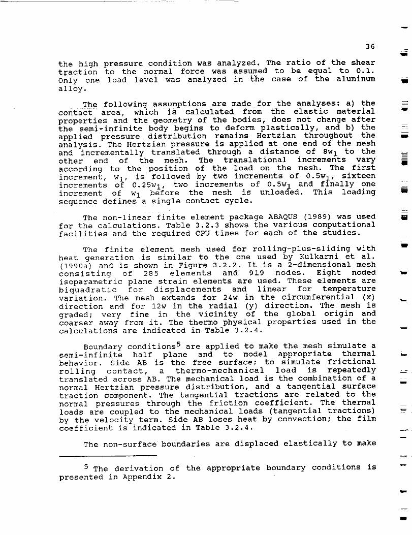
36

the high pressure condition was analyzed. The ratio of the sheartraction to the normal force was assumed to be equal to 0.i.Only one load level was analyzed in £he case of the aluminumalloy.

The following assumptions are made for the analyses: a) thecontact area, which is calculated from the elastic materialproperties and the geometry of the bodies, does not change afterthe semi-infinite body begins to deform plastically, and b) theapplied pressure distribution remains Hertzian throughout theanalysis. The Hertzian pressure is applied at one end of the meshand incrementally translated through a distance of 8wI to theother end of the mesh. The translational increments varyaccording to the position of the load on the mesh. The firstincrement, wI, is followed by two increments of 0.5wl, sixteenincrements of 0.25w I, two increments of 0.5w I and finally oneincrement of wI before the mesh is unloaded. This loadingsequence defines a single contact cycle.

The non-linear finite element package ABAQUS (1989) was usedfor the calculations. Table 3.2.3 shows the various computationalfacilities and the required CPU times for each of the studies.

The finite element mesh used for rolling-plus-sliding withheat generation is similar to the one used by Kulkarni et al.(1990a) and is shown in Figure 3.2.2. It is a 2-dimensional meshconsisting of 285 elements and 919 nodes. Eight nodedisoparametric plane strain elements are used. These elements arebiquadratic for displacements and linear for temperaturevariation. The mesh extends for 24w in the circumferential (x)direction and for 12w in the radial (y) direction. The mesh isgraded; very fine in the vicinity of the global origin andcoarser away from it. The thermo physical properties used in thecalculations are indicated in Table 3.2.4.

Boundary conditions 5 are applied to make the mesh simulate asemi-infinite half plane and to model appropriate thermalbehavior. Side AB is the free surface; to simulate frictionalrolling contact, a thermo-mechanical load is repeatedlytranslated across AB. The mechanical load is the combination of anormal Hertzian pressure distribution, and a tangential surfacetraction component. The tangential tractions are related to thenormal pressures through the friction coefficient. The thermalloads are coupled to the mechanical loads (tangential tractions)by the velocity term. Side AB loses heat by convection; the filmcoefficient is indicated in Table 3.2.4.

The non-surface boundaries are displaced elastically to make

5 The derivation of the appropriate boundary conditions ispresented in Appendix 2.

W

W

mm

I

m

m

w

%.i

w

L_

= =

w

m

Rm

Table 3.2.3 Computational Requirements

37

Case Computer CPU (hrs)

w

- 4

3-dimensional rolling

Steel

3-dimensional rolling

Aluminum

3-dimensional rolling+

slidingSteel

Cray Y-MP 6 0.5

Cray X-MP 6 1.5

Vax 3500 workstation 7 84.0

=

E

?

w

6San Diego Supercomputer Center.

7The rolling sliding calculations are in

stage; they will be implemented on the Cray Y-MP.

the development

E

L

38

A

D

IY

h

p,t,q _ V_, ////

//////I I\\\"_,\////// 1\ \\\\

C

2,_w

B

12w

ZI

111

mm

u

m

!im

m

l

B

Figure 3.2.2 Finite element mesh used for the 2-dimensional

calculations which accounted for rolling-plus-

sliding, with the resulting heat generation.

W

z

w

Table 3.2.4 Thermo physical properties for 2-dimensiona_

calculations plus contact loadinq and qeometry

39

Parameter Value

t •

w

Young's Modulus

Poisson's Ratio

Kinematic Yield Strength

Hardening Modulus

Kinematic Shear Yield Strength

Peak Hertzian pressure

Half contact width

Mass density

Specific heat

Friction coefficient

Thermal expansion coefficient

Film coefficient

Thermal conductivity

207.0 GPa

0.3

1050.0 MPa

188.0 GPa

606.0 MPa

3. 031 GPa

0.5 x 10 -3 m

7850.0 kg/m 3

550.0 J/kg °C

0.2

1.2xlO -5 m/m °C

150.0 W/m 2 °C

60.0 W/m °C

u

Z

w

4O

the mesh behave as a semi-infinite half space. The non-uniform

mechanical loads, p and t, are discretized into several

concentratedforces, each acting on an infinitesimal area.

Elastic displacements due to each of these forces are

calculated at the non-surface boundary nodes using the equations

derived in Appendix i, and the principle of superposition is

applied. For the nodes along the bottom surface, DC, both X- and

Y-displacements are prescribed while for those on the sides AD

and BC, only displacements in the X-direction are calculated

using the elastic solution. The following assumptions have been

made: (I) temperature independent mechanical and thermo-physical

properties, (2) arbitrary heat transfer coefficient h, (3) no

heat generation due to inelastic straining, (4) the bearing

material is assumed to be a continuum (metallurgical

transformations accompanying the high temperatures are not

considered).

3.3 Three Dimensional Rolling Contact of Bearing Steel

Results are presented for the loaded state in the form of

iso-contours. Given the complicated three dimensional nature of

the problem, views along all three orthogonal axes are presented,

i.e. the top view (along the z-axis), the front view (along the-

y-axis), and the side view (along the x-axis). The residual

state values are presented for a set of elements located at the

center of the mesh as a function of the depth. The stress-plastic

strain histories in the half space are also introduced. The

stresses are normalized with respect to kk, the strains with

respect to kk/G and the depth with respect to w I.

As mentioned earlier, three different load levels were used

for the pure rolling analyses. The alternating or translating

component of the stresses acting upon the half-space, is shown in

the form of stress contours for the three pressure distributions

(high, medium and low) as well as for the three possible views

(top, front and side), for the case when the pressure is half way

through the second contact. The schematic drawings included with

the figures indicate the plane where the stresses are viewed.

All figures are shown for the second pass, however results for

the first pass were almost identical.

Figure 3.3.1 shows the distribution of equivalent Mises

stresses for high, medium and low pressure 8 viewed from the top

face of the model, i.e. along the z-axis. In this figure, as well

as all other figures representing the loaded model (i.e. all

8 For the top and side views the contour plots represent the

high, medium and low pressures, from top to bottom. For the front

view the high, medium and low pressure plots are arranged from

left to right respectively.

w

m

I

m

w

g

I

M

mm

i

g

g

m

41

i

li±:

i

r-,

MISES

V__U[

I "_.4_C'02

2 "4.44E'08

"3.88Z+08

5 °!.77E+08

5 ,2.22['3S

7 ,_.56c*_g

8 _3.llE*g_

9 "3.55C-09

10 .4.00C-09

po/k =8.9

_15E5

V_LUE

1 -3.37E-g2

o3.33E-_B

3 ,5.56E-08

-:.03C,_9

5 ":.33C'¢9

5 *:,68E'Og

7 .2.COE'39

.2._3E'0£

9 -2.56_'_9

10 -_._0£-09

p:/k=66

_X

Z

_[5E5

_PLbC

; *_.22£'52

2 '2.22E'08

3 -4.44E*08

4 '5.5EE'_

5 *S.8S_-08

5 ";.;]E_C9

7 ";.3ZE'09

8 ,:.55[+09

9 "_.77E'5_

_0 "2.00E-09

Pc/k=40

I 2W2 I

I

./_

I

w

Figure 3.3.1 Contour distribution of equivalent (Mises)stresses on the surface of the mesh (viewed along

the z-axis), for high, medium and low pressures.The size of the contact is indicated in the

figure. The schematic drawing shows the viewedslice. The values are expressed in N/m 2 (Pascals).

ORIGINAL PAGE IS

OF POOR qUALITY

42

figures except those representing residual values), the load is

at the center of the mesh, and the contours are directly under

the contact pressure. The elliptical nature of the contact is

evident from the shape of the contours (the size of the

contactwidths is indicated on the figure). A constant ratio of

semi-major to semi-minor contact width was used for all the

calculations 9. The equivalent stress is as high as 3.11 GPa at

the center of the contact for the high pressure case (2.33 GPa

and 1.33 GPa for the medium and low pressure cases,

respectively). Figure 3.3.2 shows the distribution of equivalent

Mises stresses for the side view, i.e. along the -x-axis, for the

three pressure levels. It is interesting_ to note in these

figures that the contours which indicate an equivalent stress

above the kinematic yield strength (a k = 1050.0 MPa) extend up to

the surface for the high pressure case (contours 4 and higher),

reach close to the surface for the medium pressure case

(contours 5 and higher), and are completely confined to the

subsurface region for the low pressure case (contours 6 and

higher). The same observations may be made with reference to the

contours shown in Figure 3.3.3. This figure shows the front view

of the equivalent Mises stress contours for a set of elements

located at the center of the mesh, as indicated in the schematic

drawing.

The translating 3-D Hertzian pressure produces highly

complex stress distributions in the half space. This is clearly

evident in Figures 3.3.4 through 3.3.8, which show stress

contours for the second contact. Figure 3.3.4 shows the contact

stress distribution (along the z direction) on the top surface.

The contours provide evidence of the elliptical nature of the

contact, elongated along the x-axis (perpendicular to the rolling

direction). Figure 3.3.5 depicts the distribution of shear

stress, axy , near the top surface, viewed along the z-axis. Thepeak values for the antisymmetric distribution of this stress

component are present at the edge of the contact, and range from

plus to minus 166.0 MPa for the high pressure case, from plus to

minus 133.0 MPa for the medium pressure case, and from -88.8 MPa

to 77.7 MPa for the low pressure case. The most favorable

conditions for crack propagation driven by this stress component

would take place on a yz plane, i.e. perpendicular to the

surface, and close to the edge of the contact.

Figure 3.3.6 shows the distribution of circumferential

stress, avv , viewed along the -x direction. As previously

observed _ Kulkarni et al. (1990a) for the case of a contact

elongated along the rolling direction, a small region of tensile

stress develops at the surface on either side of the semi-minor

contact width. For the high pressure case, the magnitude of this

tensile stress component reaches up to 333.0 MPa. However, the

9 The ratio Wl/W 2 = 1.77.

N

M

mm

m

mm

B

Wm

i

m

J

m

m

w

g

_.__-

L

m.

=

_I5E5

_.44E_02

2 "4.4_E'08

3 "8.8BE_OB

*l. 33E-_,9

5 -1.77E'C9

7 "2.5EE*09

g "3. i IE'09

9 "3.55£-05

tO ,_.ODE+09

po/k=8.9

NISES

VS.U5

1 ,3.33E*02

2 ,3.33F-..-C8

3 *6. EF..F.-08

t • I, OC,E-C5

5 • 1.33[ "C9

7 "2.C,5E'S9

3 "2.33E'3_

9 "2.55E'09

_O -3.C0£-09

p0/k =6.6

zMISE5

VPLUE

I "2,2"_E_C2

2 "2-,22r'08 i

3 "4.44£'QS

4 ,5.56Z*C8"B.BBE'O9

iB -l.IIg-Cg

7 •]. 33E *C9 i

8 "I .55E-S9

9 * l. 77[*C.9

IO ,2.3DE'09

PO / k = 4.0

J

\ J

\ /2W2

! I

43

m

w

Figure 3.3.2 Contour distribution of equivalent (Mises)

stresses on the side of the mesh (viewed along the

x-axis), for high, medium and low pressures. Thesize of the contact is indicated in the figure.

The schematic drawing shows the viewed slice. Thevalues are expressed in N/m 2 (Pascals).

ORIGINAL PAGE IS

OF POOR QUALITY

)'T! , T _ i

ilia//;,' / i

i_i!4, Z 1 , ! i:

I ! /_

F

°**°°. ....

_ ......... _ g

('_

(,.,)

Im

i,(

/

\

44I

i

I

im

I

i

I

i

II

III

i

Iii

I

I

ORIGINAl. PAC_ IS

OF POOR QUALITYIII

m

45

t £

=

L

T

=_=

=

533

¥1_LUE

I -6.006"09

2 -5,22E'3_

3 -_ _4E*C9

4 -3.5EE*09

5 -2.gBE+_

6 -2.lI['0_

7 -i.33E'O9

8 -5,55DD8

9 .2.22E'08

P0 / k = 80

533

vRLU_

: -4.3_E-C9

2 "3 44£.C9

3 -2 BB£+OS

4 2.33D_._

5 "i .77DD9

6 -_ .22£'_S

7 "5,68E'38

@ -I.IIE,08

B •=,.4.4E-09

1?, +t .00£-Z5

P0/k=86

S33

: -3.C'CE+_9

2 -2, 55E-OS

3 -2, 11E,09

4 -: .686,3S

5 "!. 22£-05

5 -7.77£-_8

8 ":.;:r'_5

9 +5.55DCB

I0 "_. 00--. +09

P0 / k = 40

z

i

__J

/

#

I 2wa t

I

iF_w

_2

b__

m_===

w

Figure 3.3.4

ORh31NAL PAG_ i_

OF POO._ _Aik.17_

Contour distribution of direct, Gzz, stressesviewed along the z-axis (top surface), for high,

medium and low pressures. The size of the contact

is indicated in the figure. The schematic drawinqshows the observed slice. The values ar_

expressed in N/m 2 (Pascals).

46im

S_.2

VP._UE

i -5.00E,38

2 -3.8BE-08

3 -2.77E °09

4 -; .SBE*08

5 -5..5_+_7

5 +5.55E'C7

7 +i ._.E-08

8 ,2.77E+08

g .3.BSE'08

10 "S.C_OE "CB

po/k=89

L'i1

!

111

Ill'

II

S;2

-4.3:r-'38

2 -3.:IE'_8

3 -2.22E'3B

-i .33E,0S

5 -1.445,:7

5 - _.,44_.,C7

7 • ',. 3-_E"c'B

8 +7.. "_r'co

9 "3. :IC'08

10 *,I._E.OS

Po/k =6+6

IIII

l!

5_2

V_u C

a -2. _3[-3S

2 -i .44_-+:0

3 -e.BBE_G7

4 -_.33E-:7

5 -2.2Z['37

S -7.77E+_7

7 ": .33E*:8

B -I.BBE.C,8

9 -2. d,i[+C8

I0 "3._OE'_B

po/k='lO

7j 2W2

tIBIli

Figure 3.3.5 Distribution of shear stresses, Gx¥ , viewed alongthe z-axis. The figure indicates t_e size of thecontact as well as the values for the contours.The stresses are indicated in N/m 2 (Pascal). The

schematic drawing shows the portion of the mesh

under observation.

ORIGINAL P.,-'r,_- IS

OF POOR __

w

i

m

47

7

= =

r_!

I!I

==W

$22

VAL,,,--

I -5.00E,09

3 -3.56-Z'Og

4 -3.coC-Og

5 -2, 33E'09

8 -I .S_E_09

7 -1.30E'_9

@ -3._3E'C8

9 ° 3,33F..*08

tO *I .ODE*09

po/k =$.9

I -4.CCC-_£

2 -3._4C-C_

3 -2 .:@E-_9

4 -2.33C-_g

5 - ',.7i['39 :

6 -i .22_--cs i7 -5.e5C-C_8 -:.ltE-O_

g *1.44E-08 I i!O *I.SO£.Og I

i

Po/k =6._

52_

v_..j[

I -2.30E*D9

-_ .6SE*C9

3 -i. ]3E°09

5 -5.58£+08

5 -3._3E_,38

7 -3.13E.02

S ,3.33['$8

g "5.56E'08

lO *I .,SOE-09

P0 / k = 4.0

z

, " - _ .... -i _ --- .-t,......

i 2w2, l

Figure 3.3.6 Distribution of circumferential, avy, directstresses under the surface. The _ pressure

distribution has been translated halfway through

one pass. _he _"schematic drawing indicates the

slice of material under observation. The values

for the contours are in units of N/m 2 (Pascals).

ORIGINAL PAGE ISOF POOR QUALI_

48

volume of material affected by the tensile stresses is not large.

Figure 3.3.7 shows the subsurface antisymmetric distribution of

shear stress, a_ This stress component peaks at a depth ofapproximately 0 . The magnltude of this stress is, however,

almost seven times as large as the previously mentioned values

for axy. The peak values for this stress range from plus tominus II00.0 MPa for the high pressure case, from plus to minus

i000.0 MPa for the medium pressure case, and from plus to minus

555.0 MPa for the low pressure case. The most favorable

orientation for a crack to grow with this shear stress component

for driving force would be on planes parallel to the surface.

Figure 3.3.8 presents the contour distribution of axial

stress, axx , for a slice of material at the center of the mesh.There is evidence of tensile axial stress at the edge of the

contact, however, with the exception of the high pressure case

where the stress approaches 444.0 MPa, it is negligible. In all

cases though, the volume of material affected by the tensile

stress is small. Figure 3.3.9 presents the distribution of shear

stress, axz , under the contact. The peak value of this shear

stress takes place at the edge of the contact, at a depth of

approximately 0.32w I. The magnitude of the shear stress is also

larger than _xy, but smaller than ay z. The peak values are i000.0MPa for the nigh pressure case, 700_0 MPa for the medium pressure

case, and 433.0 MPa for the low pressure case. The distribution

is also expected to be antisymmetric but with respect to the

plane of symmetry of the mesh, i.e. y-z.

The plastic strain increments, dePij , for each translating

increment are used to calculate the equivalent plastic strain by

integrating them over the history of loading, based on avon

Mises yield function and for the appropriate kinematic hardening

flow rule. The equivalent plastic strain, ePeq , is thus a measureof the degree of plasticity attained at a material point. Figure

3.3.10 shows the equivalent plastic strain contours half way

through the second translation of the pressure distribution,

viewed along the z-axis (top surface). Figure 3.3.11 shows the

equivalent plastic strain distribution from a side view. The peak

plastic activity takes place in all cases at a depth of

approximately 0.25w I. For the high pressure case, the peak

equivalent plastic strain reaches values as high as 0.004; for

the other two cases the maxima are equal to 0.00233 and 0.00044

for the medium and low pressures, respectively. Figure 3.3.12

shows the distribution of equivalent plastic strains viewed along

the y-axis, it is evident that as the pressure increases, so

does the volume of material affected by irreversible plasticity.

Another indication of the degree of plasticity is the

plastic work, given by the integral of the product aij.dePijover the loading history of the material points Thls

irrecoverable work leads to damage accumulation by exhaustion of

ductility, which in turn is responsible for crack initiation and

zW

mD

U

m

l

U

u

mR

i

W

I

49

=

r

w

i

v

L=

=

i

=

$23

V_L_j_

I -2.00E+09

2 - ;. 55E-C9

3 -I.IIE+C9

-6.$6E,C8

5 -2.22E+CB

6 .2.22E'CB

7 • 5.55E +,?,B

8 • ;. I _E*Cg

g •i ,55E'C3

lO *2.C_E+09

po/k=89

S2Z

VPLJF"

1 - _. OCE - 09

2 -7.77E-_5

3 -5.55£*C,9

4 -3.33E-C8

5 "I.IIE*C8

5 "l,llE'08

7 -Z. 33E'CB

8 "5.55E*F,B

9 "7.77E*CS

iO ' ',. 5CF'+C9

Polk =6.8

523

V_LUE

I " ; . ,7,"0 E +_

2 -7,77E.08

3 -5.55E+08

5 -_. ',IE-08

6 ,!.llE-OB

7 +3.Z3E*08

8 "5.55E-38

9 -7.77E*08

lO ,; .OOE-3g

Po/k=4,0

Figure 3.3.7

ORIGINAL PAGE IS

OF POOR QUALITY'

: ; \j

,,f ._.,

I 2w2 1

Antisymmetric distribution of shear stress, avz ,viewed along the x-direction. The schematic

drawing shows the portion of the mesh underobservation. The stresses are in units of N/m 2

(Pascals).

, i " i

yii

\

i:_ /i /

ii//'/ /v

i'i/ i

¢

iJ!i i

ih/I

\

7

\\

,-_ _Z

0

,-.._ 0 0

I/1

- 0 ._ ._

X_ 0_ 0 0.._

_._ ""4 _

0 _1_

o-_o

_ _ ._O_o • _ 01

co

0

/

\

5OW

i

R

i

i

i

l

ORl611ixi._L F,4--_-

OF' POOR _ALrl'g

i

=

= :

L

L ,,'iii

I j, : "/.__..._ ',,. ',, ,, ,, ".,,

, _/ , r j i \

.. ,.-_----,...-----"/ F

\

l,,')r:= !\ \ ,

\.

\ :

x

i

ORIGINAL PAGE 18OF POOR QUALITY

m

_ _r__ _ ._ _ -" _: _ _ •_

51

Oh

t,h

b",

l<

/

\

"_ -_ 0_.- _ -,._ _

_1._ rU .I-1

_._,o• o

_4_ I _-,-I

_._

o.I_: o-1_ _0

O_

-,.-t _ _

-_ I'

_ _) _ O_ _

52

PCC0

VRL_

2 "5.55E-04

3 _.11[-03

4 ,_. B5E-03

S +2.22E-03

6 "2.77E-03

7 +3.33C-03

B .3.88C-C3

9 *4.44£-03

lO *S.OOE-03

P0/k=8.9

I

=m

i

I

PEEC

VP,LUC

2 .3.33C-04

3 -E.55£-04

4 • :. OOC-03

S "i.33C-03

S *I .E_-O3

7 "2.DOE-D3

9 .2.66£-03

_0 *3.OOE-O3

p0/k =6,6 TTIT T??ii%III

II

F

i

i

I

'_-£'.3

V%',JE

2 .5.6EE-_.5

3 *; .33E-C4

._ .2.00E-D4

5 .2.66C-04

6 .3.33C-04

7 +4. OOC-O_

8 -4.66C-04

9 +S. 33E -O't

}0 *6.00r'-04

Po/k= 4.0

_X

2w2I I

i

I .

m

I

Figure 3.3.10 Distribution of iso-contours for the equivalent

plastic strains, viewed along the z-direction. Thedimension of the contacts are indicated in the

figure. The schematic shows the slice of materialunder observation.

I

I

ORIGINAL PAGE ISOF P_ _AU_

mI

i

:,,....

_=

L .

PE_

VALUE

2 .'t.44g-g4

3 ,8.BSE-04

4_ • _.33E-03

5 "i .77E-03

B "2.22E-03

7 "2.65E-03

B +3.11C-_3

9 .3.55E-03

lO ."1.90£-D3

Po / k = ILQ i

PEE_

VR.UE

2 ,3.33C-04

3 _5.5BZ-0'I

4 "_ .30E-03

5 *I .33E-C3

E. *I .B5£-03

7 "2. 005-03

B "2._3£-03

9 "2.65£-33

I0 -3.00C-03

PO / k = 6.6

)

)

PE£3

2 *5.55E-D5

3 +I. I iE-P,4

5 +2.22E-_4

5 '2.77E-04

7 "3.33E-C4

8 "3.91]E-O4

9 "I.41{-04

lO ,5.0_-04

:_ Po/k =4.0

z

I 2W2 I

53

i

L

m

Figure 3.3.11 Distribution of equivalent plastic strains under

the surface, viewed along the x-direction. The

schematic drawing shows the slice of mesh underconsideration.

_:._ .... _,OR/GINAL PAGE ISOF POOR QUALITY

i!.... _+' t i.,

_v,_/,/'.,V /

tT I!_!!_ !Iil i,')__<1,\ d/ f/

!i!i iyi, i

¢/

o , _ i , i -

g

o

t E , , , , , , , _

g

..,+ .....

14 _ I11

_o0

-_

-,"1 _.)

_ _-_

0 :> _.P

4J rj

_',_

• ,..t tO

-,_ ,_ ,--_ tl)

¢N

r.-t

/

\

54

ORIGINALPAGEIS•" -OF_P_* _,Lrn,

g

ii

i

N

m

lIB

J

I

lib

m

i

i

lib

L

w

L

w

55

propagation, thus leading ultimately to failure. Figure 3.3.13

shows the contours of plastic energy viewed along the x-axis.

Figure 3.3.14 presents the subsurface distribution perpendicular

to the z-axis; this figure indicates that the maximum

dissipation of energy by irrecoverable plastic work takes place

at a depth of 0.3w I in all three cases. Moreover, the maximum of

plastic work occurs directly under the contact (centered with the

pressure distribution). However, the volume of material exposed

to cyclic plasticity increases with the peak pressure.

In the case of two dimensional rolling, line contact (a

rigid cylinder rolling over a flat half-space), the flat surface

remains flat during rolling and the mechanically admissible

residual stress state permits only two components, arxx and o rwhich vary as a function of the distance from the surface_ _e

deformation mechanism is one of ratchetting parallel to the

surface. In the case of point contact, which is a three

dimensional problem, all six components of residual stress can

exist, and are present. Their magnitude is not only a function of

the depth from the surface (z distance) but also a function of

their distance from the center plane (x distance). The ploughing

of the material introduces a strain gradient in the axial

direction; this region is surrounded by material which has not

been plastically deformed. Upon unloading, this material tries to

recover its original shape, thus resulting in residual stresses.

Figures 3.3.15 through 3.3.17 show the distribution of

direct residual stresses at integration points located at a

distance of 0.125w I from the yz plane, at the center of the mesh.The residual stresses are normalized with respect to the

kinematic shear yield strength, kk, and are plotted as a function

of the depth below the surface, normalized with respect to the

semi-major contact width, w I. Each plot presents the results for

the three contact pressures used in the calculations. Table 3.3.1

compares the peak direct residual stresses obtained for the

present calculations with previous values reported in theliterature.

Figures 3.3.18 through 3.3.21 show iso-contours of the half

equivalent plastic strain range for the three different loadings

(high: P0/k_9, medium: P0/k=6, low: P0/k=4) for pure rolling, and

for rolling-plus-sliding at the high load level (Fig. 3.3.21).The contours are for a slice of material located at the center of

the mesh, as shown on the schematics. Figure 3.3.22 shows a

comparison of the variation in the half plastic strain range with

depth, for the three different loads under pure rolling, and the

high load under rolling plus sliding (these values are taken at

the same locations as Figs. 3.3.18-21).

56I.i

PENCR

PCNER

2 '5.55E+05

3 +I.11£+D6

4 'I.66E+06

5 °2.22E+D6

B +2.77Z*06

7 +3.33E+06

8 ,3.eB£,_

9 *4.44E.D6

1O .5.00C+06

P0 / k = $.g

VF_LL.'E

1 - i.DOE°06

2 -5.55E,05

3 -i.11E+05

4 -3.33C,05

5 +7.77[.05

S •i. _2-S-06

7 +1.66r-06

3 +2.55C-0E_

IO '3.00E+06

Po/k=66

r \

i

g

m

J

mi

PCKCm

2 "5,55['Z4

3 *I.:]£+05

4 ,;.SG[-OS

5 "2.22_-35

6 *2.77C*_5

7 +3.33£,_5

8 "3.BBE+C5

9 -4.44E*_

P0 / W = ,I.0

_x 2W 2Y_ I I

z

Figure 3.3.13 Contour distribution of the amount of energy

dissipated as irrecoverable plastic work per unit

volume, viewed along the x direction. The contours

are in units of N.m (Joules).

ORIGINAL n_^_ ,_

P(x)R QUALITY

w

I

I

I

m

mI

=

t_

=__

i

w

57

=

L

_==

=

_4

m

=

i

PENER

V_Lb%

2 "5.55C.05

3 *:.ItE*_6

4 'I.56C*06

5 +2.22C'D6

5 "2.77E*DS

7 "3._3E_05

B .3.38C-06

9 +i._t[*06

10 -5._0C*06

PO / k = 8.9

PENE_

W_UE

I -_.OOE+06

2 -5.55C-05

3 -:.]IE*OS

4 .3,3ZE,05

5 "7,77C+05

5 ":_22E'C6

7 "I.55C-C5

8 "2.11C*06

9 '2.55E-C6

]0 .3.00E-08

PC / k = 6.6

T/' - _ i_!!

PENEa

2 ,5.55C-04

3 .1.33E.05

-2.00EOC5

5 -2.56£-_5

B .3.33Z-35

8 ,I.55E*05

9 .5.33£+G5

I0 .6.OGE*05

po/k =4.0

_X

T

_(! / t W Agh !2W 2

I I

....... : r : = =

Figure 3.3.14 Contour distribution of energy dissipated by

plastic work, viewed along the z-direction on thesl ice of material indicated in the schematic

drawing. The contours are in units of N. m

(Joules) .

OR!GINAL PAGE IS

OF POOR QUALITY

58U

W

0.04

0.02 -

0.00

-" -o.o2-l

b

-0.04 -

-O.Oe-

_'Ik_vsz/w

I

• \ __ /" e__x=x_x._-,_\ / - _

ANo\ _

Legend

p./k.--8.g3

• p_a,-e.se

X p;_;-,3.g8

-0.08 I i _ I

0 0.4 0.8 1.2 1.e 2

_W

g

m

U

i

mm

iqm

mm

111

Figure 3.3.15 Distribution of residual direct stresses at the

center of the mesh in the axial direction

(normalized with respect to the kinematic shear

yield strength) as a function of the depth

(normalized with respect to the semi-major contact

width). Results for the three different loadings

are indicated in the Fig.

w

mm

59

%..

= :

(: '/k_vsz/w

0.02 -

.'..°-1o.oo X-X-XX- - _ "_ _\ _, X_=,,,,=,,,,=^

:;.. // .._ / _ _,o.nox ,.-_\ / / _,,.,,,.-,,.,,,v" % / / • _,',,_

-oO\ \ • / X p./k.-S.Oe

.o.oo. ON • /-0.01 -

-0.10 , i i

0 0.4 0.8 1_ 1.6 2

z/w

mw

Figure 3.3.16 Distribution of residual direct stresses at thecenter of the mesh in the circumferential


kinematic shear yield strength) as a function of

the depth (normalized with respect to the semi-

major contact width). Results for the three

different loadings are indicated in the Fig.

PRECEDING PAGE BLANK NOT FILMED

Table 3 3.1 Direct residual stresses

61

Reference arxx aryy arz z

Groom (1983) -150

Bower and Cheesewright(1988) -150

Bhargava (1988), Po/kk=5 -7O

McDowell and Moyar(1986) NA

Kulkarni I0 (1990a), Po/kk=9.2 -115

Present Work:

Po/kk=8.93 -3614

pure rolling Po/kk=6.59 -3219

Po/kk=3.98 -167

roll. + slid. Po/kk=8.93 -45ii0

-180 -30

-220 -60

-63 NA

-212 NA

-180 -40

Um

I

I

-59 -16_=_

6 14 w

-56 -16 --

7 18U

-32 -7

5 6

-121 -68

247 58

Note i:

Note 2:

The peak compressive and tensile residual stresses are

presented for the three different contact pressures

under pure rolling, and also for the rolling plus 0.2

percent sliding case.

All the stresses are expressed in MPa, and for the

present work, for the second pass of the load.

m

W

U

N

I0 The contact ellipsoid was elongated along the rolling

direction for this 3D calculation.

U

W

m

=

w

62

_===

z z:

L

w

L

N

,.I-

_4

i.O

0

1.60_

! !,.e 1.6 ,.,' ,.= i.o..... X/H

m

w

Figure 3.3.18 Iso-contours of the half equivalent plastic strain

range for pure rolling with high loading (P0/k=9).The contours are for a slice of material located

at the _c4nter of -the mesh, as shown on the

schematics. Strain values are shown magnified X10 3 .

m

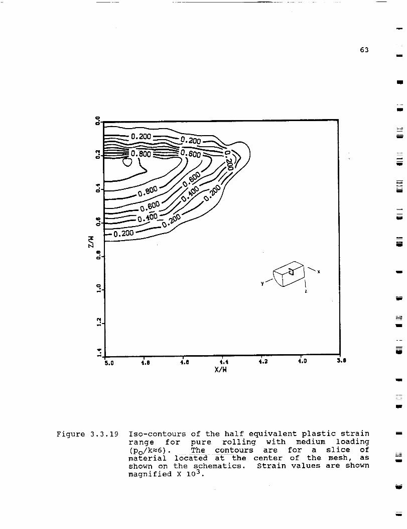
63

Z

N

o

d-

o.

N

z

5.0 .S B _.4 _.2 4,0×/N

JoB

J

g

i

_I

J

mm

J


range for pure rolling with medium loading

(Po/k=6). The contours are for a slice ofmaterial located _'&t_the center of the mesh, asshown on the schematics. Strain values are shown

magnified X 103 .

l

=_

mJ

U

64

0"

"It

N

IDd-

o

...e-

Z

i i l i I

5,0 4,8 4.6 4,4 4.2 4.0 $.8

w


range for pure rolling with low loading (Po/k=4).The contours are for a slice of material located

at the center of the mesh, as shown on the

schematics. Strain values are shown magnified X103

65I

J

a.

N

!

S.O 4.8

Z

|' ! | |

4.0 4.4 4.2 4.0 5.8

_H

I

mwm

mi

!

1Ira

Ulm'

meg

_r

mm

I


range for rolling-plus-sliding with high loading

(Po/k=9). The contours are for a slice ofmaterial located at the center of the mesh, as

shown on the schematics. Strain values are shown

magnified X 103 .

ml

m

i

i66

L

-_J

=

"- 24.0i

0.00

_eqP/2 vs z/w

Legend0 p,/K_-g.g8 r

[] p./K.--O.§9 r

0 p./K_--8.93 r

• pJK_"8.93 r+e

0.2 0.4 0.6 0.8

z/w

w

qmm

w

Figure 3.3.22 Comparison of the variation in the half plastic

strain range with depth, for the three different

loads under pure rolling, and the high load under

rolling-plus-sliding (these values are taken at

the same locations as Figs. 3.3.18-21)

67

3.4 Three Dimensional Rolling Contact of Hardened Aluminum

The Mises equivalent stress distribution for the Aluminumproperties is shown in Figure 3.4.111 • This figure shows theequivalent stress contours on two different sections of the meshin the vicinity of the contact, as indicated in the schematicdrawings. The peak value of the equivalent stress occurs at adepth of approximately 0.5w below the surface.

Figure 3.4.2 illustrates the equivalent plastic straincontours underneath the contact. The equivalent plastic strain,cPeq , is obtained by calculating the equivalent plastic strainincrement, dEPea, for each incremental pressure translation, andintegrating it _ over the entire loading history, it is acumulative measure of plasticity in the half space. Plasticstrain activity extends to a depth of approximately lw below thesurface and the peak plastic strain is located at a depth ofapproximately 0.4w, as shown in Figure 3.4.2.

The distribution of the continuing cyclic plasticity duringthe first and second contact sequences is shown in Figure 3.4.3.This shows the variation with depth of equivalent plastic strainrange, _£P, which peaks at a relative depth of z/w = 0.45. The

magnitude of _P is non-zero up to a relative depth of z/w = 1.5

for the first contact. However, for the second contact (or

steady state), £P extends only to a relative depth of z/w = 1.0w.

The magnitude of peak EP remains essentially the same between

the first and the second contacts.

The residual stresses developed as a result of plastic

deformation of the rim at the end of the second contact are

illustrated in Figures 3.4.4 through 3.4.7. Contours of axial,

ax, and circumferential,3 [{[ residual stress contours are shownin Figures 3.4.4 and .4 Residual stresses become tensile

very close to the surface, within a relative depth of z/w = 0.2.

Figures 3.4.6 and 3.4.7 illustrate the variation of _x and awith relative depth. Peak residual stresses are compressive an_

are located at approximately z/w = 0.9.

The cyclic shear stress-shear strain history experienced bythe model for the two contacts is shown in Figure 3.4.8. The

point for which the stress-strain values are obtained is located

at a relative depth: z=0.4w. The non-fully reversed hysteresis

loop for the first contact is fully reversed for the second

contact. Thus the idealized ELKP material behavior allows no

ratchetting or unidirectional accumulation of plastic strains.

The permanent microstructural damage in 7075-T6 alloy is

Ii The distribution of individual

components are presented in Appendix 3.

stress and strain

m

BJ

m

I

g

L..

mmm

w

I

u

W

68

=

p

w

W

w

m

y --x_7

1 +0.00E+00

2 +7.00E+07

3 +1.40E+08

4 +2.10E+08

5 +2.80E+08

6 +3.50E+08

7 +4.20E+08

8 +4.90E+08

9 +5.60E+08

i0 +6.30E+08

ii +7.00E+08

1 +0.00E+00

2 +7.00E+08

3 +1.40E+08

4 +2.10E+08

5 +2.80E+08

6 +3.50E+08

7 +4.20E+08

8 +4.90E+08

9 +5.60E+08

i0 +6.30E+08

ii +7.00E+08

Figure 3.4.1. Contours of von Mises equivalent stress on two

different sections of the mesh (the sections are

schematically indicated by the side of each

figure). The numbers on the individual contours

represent different equivalent values of thecontours.

w

69l

zmm

U

J

1 -i. 00E-03

2 -7.00E-04

3 +4.00E-04

4 +I. 00E-04

5 +2.00E-04

6 +5.00E-04

7 +8.00E-04

8 +I. 10E-03

9 +1.40E-03

i0 +1.70E-03

11 +2.00E-03

I

J

B

m

J

m

J

U

Figure 3.4.2 Equivalent plastic strain contours

the plastic strain history as

ellipsoid completes one translation.

representing

the pressureI

J

i 7O

w

H

=--

=

_ +

-0" I

-L5£1.

N

B£o

Z

-2

-2.5

-3

-35

0 I CONTACT

z_ If CON'[ACTS

o.o 5.0 m.o ;5.0 ,'o.oEquiv.Plastic Sfr.Amplifude, A_'/2 "10-"

m

w

Z_

Figure 3.4.3 Variation of the half-equivalent plastic strain

range, plastic strain range, _p/2, with

normalized depth, for the first and secondcontacts.

z

w

711

l1

I

! !

i

z_10 9 ,

4 ", 2 I

1 -3.00E+072 -2.40E+07 7

3 -1.80E+07

4 -1.20E+07

5 -6.00E+06

6 -4.47E-07

7 +6.00E+06

8 +1.20E+07

9 +1.80E+07

I0 +2.40E+07

II +3.00E+07

1

J

i

1

i

Figure 3.4.4 Contours of the out-of-plane (or axial) residual

stress, arx . The stress values are tensile close

to the rolling surface (as indicated by the

contour levels 7 through ii).

1

1

1

1

72

w

w

I

1 -5.00E+07I

2 -4.30E+07 I

I3 -3.60E+07

4 -2.90E+07I

5 -2.20E+07 I6 -1.50E+07 i

!7 -8.00E+06

8 -I.00E+06 !I

9 +6.00E+06 i

I0 +1.30E+07 IIi +2.00E+07

Figure 3.4.5 Contours of the circumferential residual stress,

a rv. The stress values are tensile close to the

roiling surface (as indicated by the contour

levels 9 through Ii).

73I

m

I

-0.5 -

_4

.2-- -I-5 -

C.¢

_4

0 -2-

E&.

oZ

-Z.S -

-3

+_'- !

I/ I

° i

I ii

!

' /Legend

/t C3 NTACT

J

• IICONTACT , /

Z;

I

,/-3.5

-O.t5 -0.10 -0.05 0.00 0.05 0.I0

Nor_oiizeo _esidual S_SS . c,/k<

I

I

U

g

I

I

w

Figure 3.4.6 Variation of the out-of-plane (or axial) residual

stress, arx, with normalized depth. The values of

arx are obtained from integration points locatednear the middle of the mesh, where the effects of

the boundary are not significant.

I

i

Hg

I

74

w

" -0-5 -

-!

I"4

--" -I-5

Nw

-2-E

Z

-15

St

\

Legend

t CONTACT

• IICONTACT

r

!

f

i

J

/-0.15 -0.I0 -0,05 0.00

Normalized Resicual S_ress, _./k,

0.0_

w

Figure 3.4.7 Variation of the circumferential residual stress,

arv, with normalized depth. The values of ory areobtained from integration points located near the

middle of the mesh, where the effects od the

boundary are not significant.

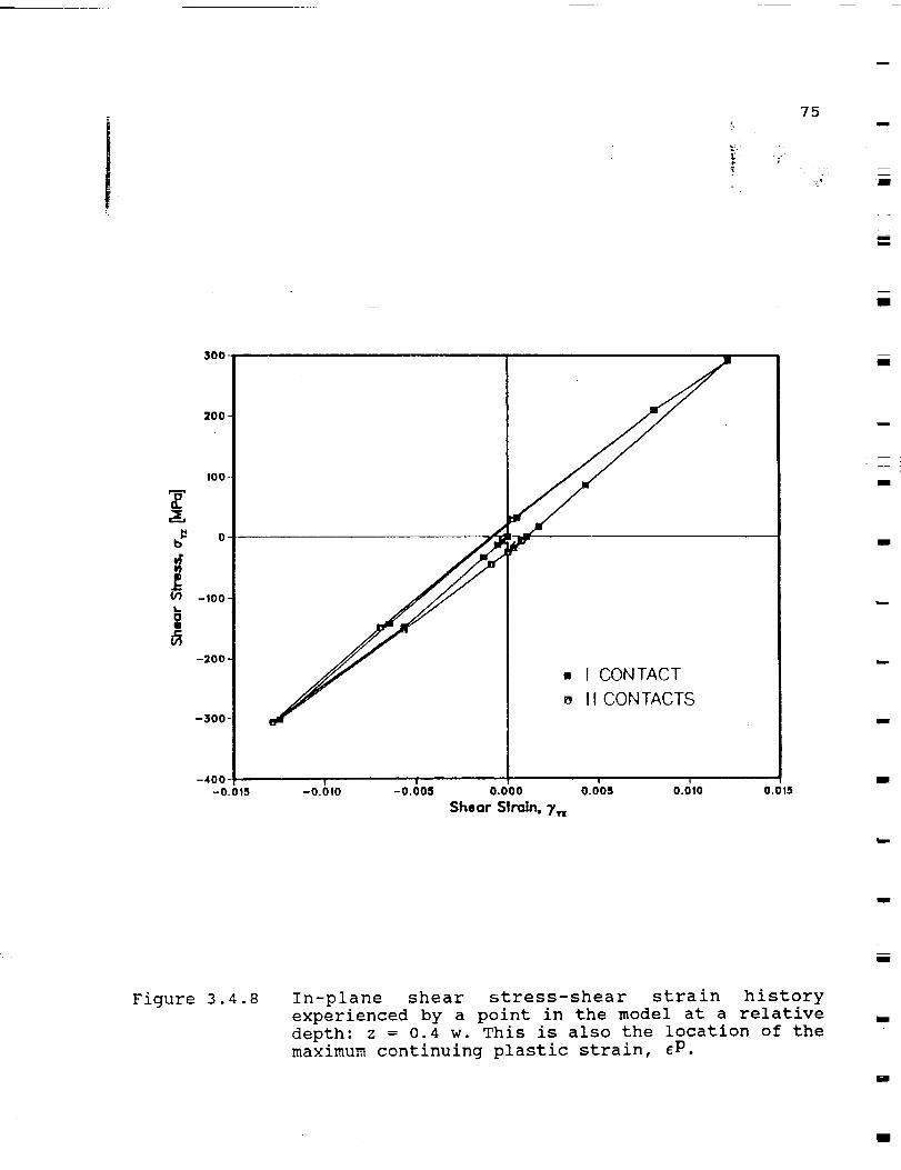
75£

i

mg

I

300

200 _

I00.

0-'

-tO0-

-200-

-300 -

• I CONTACT

. II CONTACTS

' ' O' '-O.OtO -O.OOS 0.000 O. OS 0.010 0.013Shear Strain, T.

I

I

I

I

I

I

Figure 3.4.8 In-plane shear stress-shear strain history

experienced by a point in the model at a relative

depth: z = 0.4 w. This is also the location of themaximum continuing plastic strain, cP.

mI

m

i

I

T

m

m

76

caused by continuing plasticity in the rim. The damage is

characterized by the early formation of slip bands underneath

the contact, resulting in a gradual destruction of the grain

structure followed by sub-surface crack initiation. As

illustrated in Figures 3.4.9 and 3.4.10, the shape and the extent

of microstructural damage correlate very well with the equivalent

plastic strain distribution obtained from finite element

calculations.

Sub-surface cracks occur within the plastic zone at depths:

0.i _ z/w S 1.2 underneath the running track (here, the

normalizing parameter is the semi-minor axis of the contact

ellipse, w = 0.102 mm). The distribution of sub-surface cracks

as a function of depth is shown in Figure 3.4.11. The equivalent

plastic strain variation drawn to the same scale is also shown in

Figure 3.4.11. While the extent to which cracks occur below the

surface correlates well with the extent of continuing

plasticity, the majority of the cracks do not occur at z/w = 0.4

where the plastic strain peaks. Instead, a large number of

cracks are found closer to the surface at z/w = 0.20. The

distribution of crack length below the surface is shown in Figure

3.4.12. Again, the longest cracks are located at z/w = 0.20,

while the average length Of cracks at z/w = 0.40 is approximately

10x smaller. A plausible explanation of the high occurrence of

long cracks at z/w = 0.20 from the surface is that the

compressive residual stresses decrease in magnitude at this

depth. For instance, the circumferential and the out-of-plane

residual stress distributions, illustrated in Figure 3.4.12 shows

that high levels of compressive residual stresses at depths: 0.30

z/w _ 1.2 gradually diminish and become tensile at depths: z/w

0.2. Therefore, the process of crack initiation and growth

resulting from peak plastic activity is impeded by the presence

of high compressive residual stresses.

The following sequence of events occurs in 7075-T6 aluminum

before the final spall failure. Directly underneath the contact

at depths: z = 1.0w, slip lines gradually develop as a result of

continuing cyclic plasticity in the initial stages, i.e., N S 103

cycles. These slip lines probably represent plastic activity in

the primary slip systems. As the plastic damage continues, i.e.,

103 S N _ 106 , more slip systems are activated. Gradually the

slip bands become less discrete giving a destroyed appearance to

the grain structure. The only visible slip bands at this stage

are either very close to the surface: z/w _ 0.i, or at the outer

edges of the damaged region: z/w _ 1.2, where the plastic strain

tapers off. Small cracks nucleate within the damaged region:

0.i0 _ z/w _ 1.2. Smaller levels of compressive residual stress

favor both the initiation and the growth of cracks at z/w = 0.2.

As one of the crack branches reaches the surface, a chunk of

material breaks off, leaving behind a spall pit. As this

process continues, the spall pit grows larger and deeper into the

rim. These steps are schematically illustrated in Figure 3.4.13.

m

77J

4,j

o

i -I.OOE-03

2 -_.30E-043 -4.00E-04

4 *I.00_'04

5 o2.00E-04

_5.00E-047 o|,QOE-04

| -1.10[-03

9 _1.40E-03I0 -1.70E-03

4

"% % "." "" a

a

.o

i

b

1 -1.00E-03

2 -7.00E-04] .4.00E-04

4 _2.00E-04

5 ,2.00[-04

.5.00E-047 .$.00Z-04

| +L.10[-032 *I.40Z-03

10 _1.70E-03

II _2.00E-03

_'-_ • V I

5 ? 8

Figure 3.4.9 Comparison of plastic strain contours obtained

from finite element calculations and the(a

microstructural changes produced by rolling:

after 103 contacts, and (b) after 2.3 x i0

contacts. The microstructure and the adjoining

contours are shown on the same Scale•

ORIGINAL PAGE 15

OF. POO 0 U UTV

"18

E_

r

m

L_

i

_ o

4

i-|

o °

_ O

"_

,__ 0

_o '_o_

_. _ 0

I

,-_ O _'_ _

°_- 4_ .-_ .,_

0 "_ "_

_'_ r/', ,.-_ 0 ,'-"_

0

@

D_

ORIGINAL PAGE IS

OF POOR QUALITY

w

79Bn

0O

NUMBER OF CRACKS

10 20 30I I I 0

ll'

g

I

cLw

0

0

F//

/

/

/

A

I I I

5 t0 15

A E_2 x 104

1,,0-0

_0

N

g

il

IIlll

i

m

I

J

il

Figure 3.4.11 Distribution of sub-surface cracks with depth

below the surface. The variation of the equivalent

plastic strain amplitude, _P/2, is indicated bydashed lines.

b--.

8O

w

= =

=

w

L

----4

AVERAGE CRACK LENGTH, #M

I

,\\ I

%

D.

I

II

I1II

I1I

IIIIII

I

\

\

200 4OO1 I

I\

LL

//

///i /

!

,/o

\1

\

\\ \

P T/

///

/

I I

* 0.1 0 -0.1 -O2

RESIDUAL STRESS, cr-//KK

-0.5

i

Figure 3.4.12 Distribution of sub-surface crack length with

depth below the surface. The variation of the

axial (Ox) and circumferential (ay) residualstresses are indicated by the dashed llnes.

81

=_

m

g

M

@)/

m

g

m

m

II

m

I

_: :±

Figure 3.4.13 Schematic diagram of spall formation in 7075-T6

aluminum. _

I

w

L =

w

w

L

r_

Em

= =m

62

The implication of these results is that compressiweresidual stresses retard the process of sub-surface crack

nucleation and growth even in the presence of continuing

plasticity. Hence, longer lives can be obtained by artificiallyinstalling residual compressive stresses in a relatively shallow

region under the surface, i.e., z/w S 0.25, or by altering the

properties of this shallow layer. The rolling cantact

performance is strongly determined by the cyclic stress-strain

response of the material, In spite of the microstruct%Lral

differences between bearing steels and 7075-T6 aluminum, the

cyclic stress-strain response of these two materials is

qualitatively similar. Therefore, the extension of therelationship between residuil Stresses, cyclic plasticity and

sub-surface crack nucleation from 7075-T6 aluminum to bearingsteels is justifiable.

Some of the major limitations of the present work are

noteworthy. Cyclic axial tests do not reproduce the non-

proportional straining and rotation of principal shear directionsthat result from repeated rolling contact above shakedown. When

the principal shear directions do not rotate, the cyclic damage

is limited to a fewer number of favorably oriented slip systems

and the damage is more intense. In addition, the absence of

hydrostatic stresses and the larger stressed volume shorten the

life in cyclic axial fatigue tests. This is a likely explanation

for the 103-fold difference between the rolling contact life and

the cyclic axial tests. Also, in 7075-T6 aluminum, the

precipitate particles are important contributors to strength 12.

However, the effect of particles is ignored in the currentstudy.

Future extension of the current study must treat (a) the

strain rate effects on cyclic stress-strain response, (b) non-

linearity of the kinematic hardening behavior, (c) the effect of

particles, (d) thermal effects, and (e) anisotropy and texture

effects. More work is needed to characterize the process of slipband appearance at a sub-micros£ructural scale.

3.5 Two Dimensional Rolling-Plus-Sliding with Heat Generation

Figure 3.5.1 shows the normalized residual stresses as a

function of normalized depth, y/w (after unloading followed by

cooling to the ambient temperature). Both the axial (az) andthe circumferential (Cx) stresses are found to be tensile up to

a depth of approximately 0.5 y/w. Figures 3.5.2 and 3.5.3compare the circumferential and axial residual stresses

12 Indeed, during the axial fatigue tests, a noticeable

difference between the elastic slope in tension and compression

was observed. This is probably an effect induced by theprecipitate particles.

83

respectively for the thermo-mechanical and mechanical loading

cases. Significant differences in magnitude and nature are

observed. Fig. 3.5.4 presents theresidual equivalent plastic

strain contours for a section of the mesh, and Fig. 3.5.5 shows

the residual equivalent plastic strain variation with depth.

Peak plastic activity occurs slightly beiow £he surface. Figure

3.5.6 shows a section of the residual state of the mesh (after

cooling to the ambient temperature). The surface temperatures

half way through the passes are shown in Fig. 3.5.7. The

temperature distribution is asymmetric about x/w = 0.0. Fig.

3.5.8 shows the temperature contours half way through the third

pass. Figures 3.5.9 and 3.5.10 present the hysteresis loops for

the second and third passes, respectively. The loop is found to

be closed after the third pass (second thermo mechanical pass)

indicating fully reversed plasticity.

The analyses reveal that the incorporation of ELKP material :

properties greatly reduces the plastic strains generated compared o_i

with those resulting from perfect plasticity. The p@ak residual

equivalent plastic strain (CD) obtained here, 2.5xi0 -3 (Po/k=5.0,

_=0.i), is equal to 1/25 oT the value obtained by Kulkarni et

al. (1989): 6.0x10 -z (Po/k=5.0, _=0.i), for elastic perfectly

plastic behavior under the same operating conditions. From Fig.

3.5.5 it can be seen that heating does not have a large effect on

the residual strains, but the peak strain occurs at a lesser

depth. Further, it should be noted that no plastic strains

extend beyond a depth of 2w (see Figs. 3.5.4 and 3.5.5).

A similar trend is seen for the residual stresses. The

normalized stresses are found to be tensile, consistent with the

findings of Kulkarni et al. (finite element model, 1988), and

Muro et al. (X-ray measurements, 1973), But the magnitudes are

far smaller than those obtained by Kulkarni et al. who reported a

peak normalized circumferential residual stress of 1.7, clearlydue to the difference in material properties. The residual

stresses are found to be highly tensile and less compressive as

compared to the non-heating case. The ratio of peak tensile

stress to peak compressive stress is close to 2.5 for circum-

ferential residual stresses, and 2.0 for axial residual stresses.

A value of 2.0 has been reported by Muro et al. (1973),

determined by X-ray measurements (see Figs. 3.5.1 and 3.5.2).

The peak circumferential residual stresses are found to be about

1.4 times the peak axial residual stresses (Fig. 3.5.3). It

should be noted that the residual stresses vanish at a depth of

2w as do the residual strains. The highest temperature after

three passes is found to be 590 C. The temperature increment per

pass decreases with each pass but the thermal steady state is not

reached (Fig. 3.5.7). The temperature contours half way through

the third pass show high temperatures away from the position of

the load in the direction opposite to the translation of the

load. Temperature gradients are seen to vanish after a depth of

0.5w. This steep temperature gradient produces very high

m

m

i

mm

m

l

i

D

mN

J

i

u

m

w

84

= =

L

= =

=

r RESIDUAL STRESSES

w

u

=

L"W

W

W

m

m

i)

0.10-

0.05 -

0.00

-0.06

-0,I0 '

o

\

o'.0

I Legend

o sxx/r.• SZZ/T

i ,.'5 ; _.'6 _ s.6:_ Y/w

=

E

w

m

Figure 3.5.1 Normalized residual stresses as a function of the

normalized depth, y/w. Mechanic unloading followed

by cooling to the ambient temperature.

85I

m

O.lO -

O.OO -

0.00 -

-0"05 1

-o.lot0

RESIDUAL CIRCUMFERENTIAL STRESSES

I Legend I

o With Hea_._ I

• w<th+ou_H,atI

\\

i\ll/--ll_l

m

1.'8 + z.'+ + s.5Y/w"

i

U

u

U

m

m

g

m

Figure 3.5.2 Circumferential

thermomechanical

mechanical loading

residual stresses for

(open symbols) and pure

(filled symbols).

m

N

w 86

= c

AXIAL RESIDUAL STRESSES

_---7_w

w

W

m

0.10 !

0.08-

0.00 -

0.04 -

O.OZ -

0.00

-0.02-

-0.04 -

-0.00 -

-0.08 -

-O.|O

0

_MI M

Legend }

• Without ._o_.1

Figure 3.5.3Axial residual stresses for thermomechanical (open

symbols) and pure mechanical loading (filledsymbols), for a point located at the center of themesh.

87U

m_p

m

n

u

VRLU[

I *4.00E-IO

2 -4.00£:04

3 -8,00E-04

4 41.20E-03

S "1.60£-03

5 ,2.00E-03

7 *2.40E-03

8 ,2.00£-0:]

g ,3,20E-03

I0 +:].60E-03

|I ,4.00[-03

V

u

mmm

mi

m

e=mm

Figure 3.5.4 Residual equivalent plastic strain contours.

J

i

w

88

w

w

m

=

L-.

,,-.¢ 80.0

20.0

0 0.2

EQUIVALENT PLASTIC STRAINS

Figure 3.5.5 Residual equivalent plastic strain variation with

depth for a point located at the center of the

mesh.

=

89I

u

m

w

r rT--rz--*-T---T-' T-=-:

i t I I

k + +___+

\, ,\,\[ X I i

--G--\+--\-+ --_x• t \1

-\-+-\- +-V---_ +-2_ _,

_

I I } I },i L L± . I J

R

B

W

W

u

ill

-21I

m

m

m

t

Figure 3.5.6 Deformed residual Configuration of the mesh after

cooling to room temperature. Magnification factor

x590.

mW

m

m

9O

w

°

o

SURFACE TEMPERATURES

600-

GO0

/

300

100-

0

x/w0.5 i ,.'5 2

w

Figure 3.5.7 Distribution of surface temperature

through the pass, for different passes.

halfway

-_ _r_- _

91i

N

i

VALUE

1 +7._-05

2 +7.00C,01

3 +I.10C+02

4 +2,10C*02

5 ,2,_0C+02

6 ,3,50C+02

7 +4._0C+02

8 "4.g0C+02

9 '5.GOE'02

I0 "6.30C+02

II "7.00C+02

m

W

m

I

W

m

I

J

Figure 3.5.8 Temperature contours half way through the third

pass.

J

m

i

92

w

w

= ,

=

=--

HYSTERESIS LOOP,PASS 2

0.0'04 O.O'OB O.O'OB 0.010

L_

Figure 3.5.9 Hysteresis loop, shear stress versus shear strain,

for the second pass

m

=_

93

g

m

HYSTERESIS L00P,PASS 3

1.0

1-

0.6-

0"

-6.6 -

-|

-1.6-0.i

, m, i

i i i i i 01hi2 -6.016 -0.006 -6.606 -0.004 -0.002 6.006 O. 02StlEAR STRAIN

o.o'o, 6.6'o6 o.o'oe o.+,.o

im

mm

t

Im

i

im

w

ml

=J

l

Figure 3.5.10 Hysteresis loop, shear stress versus shear strain,

for the third pass

m

m

w

i

L

w

L

w

w

L •

L_

i

w

94

compressive stresses. This is followed by a nonuniform thermal

contraction during cooling which appears to be the reason for the

residual tensile stresses. These transient residual tensions

(due to the translating thermo-mechanical load) suggest a

possible mechanism for thermo-cracking. The hysteresis loops show

that plasticity is fully reversed after two passes as reported

by Ham et al. (1989).

Temperature dependence of thermo-physical properties is

complicated and difficult to implement. Of the thermal

properties, r, the thermal diffusivity, usually co-varies with

the thermal conductivity, K, at intermediate and high tempera-

tures. As a rule p decreases and c D increases with increasing

temperatures, while k increases or aecreases with temperature,

depending on the material. The most important thermal parameter

is h(T) , the coefficient for forced convection (film

coefficient). In forced convection h(T) varies from I0 to 104

W/m 2 K, and depends on geometry, flow conditions and physical

properties. An attempt at a boundary layer analysis to solve the

heat transfer problem and define h(T) for a specific contact

situation is recommended. Of the mechanical properties, E,

Young's modulus, decreases, while v, Poisson's ratio, increases

with increase in temperature.

Accounting for the changes in mechanical properties with

temperature is recommended for further study; the material will

soften at high temperatures and this could significantly alter

the residual stresses and strains.

3.6 Conclusions

Three dimensional finite element calculations of repeated

frictionless rolling contact have been carried out for ELKP

properties of an AISI 440C bearing steel, at relative Hertzian

pressures of Po/kk _ 4.0, 6.6 and 8.9, using the geometry of the

3-ball-rod contact fatigue testing machine. The subsurface

stresses, plastic strains, residual stresses and plastic work

done are evaluated. Equivalent stresses above the kinematic yield

strength extend to the surface only for the highest load level.

The peak equivalent plastic strain occurs at approximately 0.25w 1

(Wl/W 2 = 1.77) for all load cases; the values of these strainsare 4 4x10 -4 2 33xi0 -3, and 4 0xl0 -3, for the low, medium and

high loads, respectively.



properties of the 7075-T6 aluminum alloy, at a relative Hertzian

pressure of Po/kk _ 5.7, using the geometry of the 3-ball-rod

contact fatigue testing machine. The subsurface stresses, plastic

strains, and residual stresses are evaluated. The peak plastic

strain amplitude, _£Pmax/2 = 1.6x10 -3, occurs at a relative depth

of z/w = 0.4 below the surface. Peak residual stresses obtained

D

95

are arx(max) = 26.4 MPa, and ary(max) = 39.7 MPa, occuring at arelative depth of z/w = 0.9.

; _ } ;=7 = ; : --- _ . _ :i

Two dimensional finite element calculations of repeated

rolling-plus-sliding contact have been carried out for ELKP


pressures of Po/kk = 5.0. Plastic strains, residual stresses and

temperature distributions are presented. Plastic strains are

shown to be considerably lower for ELKP properties than for an

elastic-perfectly-plastic material (Kulkarni et al., 1989).

Steep temperature gradients close to the surface produce high

compressive stresses; the ensuing cooling causes residual tensile

stresses, a possible mechanism for thermo-cracking. Thermo-

mechanical behavior is highly dependent on the material

properties, which also may be temperature dependent. A more

precise definition of these properties, especially the thermal

film coefficient, is recommended.

l

m

mm

m

!

w

Gc

Im

mm

m

c

=:_

u

W

mm

U

m

m

D

m

m

w

w

L_w

E

h •

Elw

=_

96

• EVALUATION OF THE FRACTURE MECHANICS DRIVING FORCE FOR SPALL

GROWTH

4.1 Background

This section reviews and extends calculations of the frac-

ture mechanics driving force for cyclic crack growth under

rolling contact (see Keer and Bryant, 1983, O'Reagan et al.,

1985, Bastias et al., 1989, and Hanson and Keer, 1991, for

reviews of the problem). Observations of the spall process in

440C samples, described in Section 5.4, as well as observations

of spall damaged HPOTP bearings (Bhat and Dolan, 1982, 1983),

indicate that the spalls nucleate close to the surface. The

number of cycles needed by surface-breaking, micron-size crack

nuclei to grow to a spall is one component of the contact life.

The analysis of the growth component is a difficult task,

particularly for the conditions in the HPOTP bearing. First,

there are several features that can add to the K - crack

growth driving force produced the Hertzian stresses. These

include stationary pressure spikes arising from surface irregula-

rities, the pressure of lubricant in the crack cavity, centri-

fugal and tensile residual stresses superimposed on the Hertzian

stresses and thermal stresses. The contributions from these

sources are not necessarily in phase. Secondly, there are Mode

I, II and iII contributions to the driving force whose combined

effect is difficult to predict. Thirdly, the driving force is

modified by the crack face friction and the non-planar crack

profile, features that are difficult to quantify. Fourth, only a

few studies have examined the actual 3-dimensional crack con-

figuration (Kaneta and Murakami, 1991, Hanson and Keer, 1991).

Finally, analyses of the driving force are difficult to test

because the centrifugal stresses, lubrication and thermal condi-

tions in the HPOTP bearing are not reproduced in the 3-ball-rod

testing machine.

The sources of driving force are examined more fully in

Section 4.2. A new analysis by Bower (1989) for a 2 dimensional

surface breaking C rac_ _i£h entrapped iubricant is applied inSection 4.3 to define the fracture mechanics driving force for

conditions of interest. Results of driving force calculations

for the different s0urces are Compared in Section 4.4. The

corresponding threshold crack sizes for growth are examined in

Section 4.5. Actual measurements of the growth life are

presented in Section 5.4. Fracture mechanics predictions of

crack growth are compared with the measurements in Section 6.3.

4.2 Contributions to the Spall Growth Driving Force.

4.2.1 Hertzian Stresses. Under pure rolling contact, the

Hertzian stresses -- those associated with perfectly smooth,

J

97

idealized contacting surfaces -- are largely compressive and, by

themselves, fail to generate a Mode I crack driving force 13. Low

levels of tensile stress are generated close to the surface for

the case of rolling-plus-sliding with friction but these are not

likely to produce significant Mode I K-values for small, as-

nucleated cracks. Two-dimensional treatments of sub-surface

cracks (O'Reagan et al., 1985) show that the cyclic shear

stresses generated under rolling contact do produce Mode II and

Mode III K-values. The peak values occur well below the surface

at relative depths y = w (where 2w is the contact width) provided

crack face friction is ignored. However, even the peak values

are modest because the friction and interlocking between the

rough crack faces impede the crack face sliding. For lubricated

contact, the Mode II and Mode III K-values diminish as the

surface is approached. This is also true for surface-breakinq

cracks. Keer and Bryant (1983) find that the K-values of 2-

dimensional surface-breaking cracks are very small for crack

lengths just beyond the nucleation stage, i.e. a = i0 _m. In

general, the driving forces produced by 3-dimensional cracks are

even smaller (Kaneta and Murakami, 1990). The conclusion to be

drawn from this is that the mechanical effects of pure rolling

contact of idealized smooth surfaces do not promote the growth ofmicron-size surface or near-surface cracks. Other contributions

to the K-driving force must be considered to account for the

formation of spalls.

4.2.2 Stationary Pressure Spikes from Surface _rreqularities.

The analyses of Goglia et al., 1984, de Mul et al., 1987, and

Elsharkawy and Hamrock, 1991 reveal that small, sub-microns-size

irregulaities in the running track surface, i.e., asperities,

dents and grooves, produce large, local perturbations of the

Hertzian pressure. These are in the form of narrow, stationary

pressure spikes that rise and fall as the contact passes over the

asperity. The spikes can be expected to assist the nucleation of

near-surface cracks and then intensify the KII- and KII I-

values generated, thereby facilitating their growth until they

attain a size comparable to the dimensions of the surface

irregularity. Evidence of this is contained in early work

showing direct relations between surface roughness and contact

life (Soda and Yamamoto, 1982), the deleterious effects of debris

dents (Lorosch, 1982) and the measurements reported in Sections

5.4 and 5.5. No work has yet been done to analyze the contribu-

tions of stationary spikes to the crack growth driving force.

4.2.3 Entrapped Lubricant. Experiments by Way (1935),

Dawson (1961), and Clayton and Hill (1986) show that spalls do

13 The Modes I, II and III correspond with the opening mode,

in-plane mode and out-of-plane mode of crack loading, respective-

ly.

W

M

mu

u

m

m

_ImW

m

w

m

mB

i

r

w

v

w

98

not form in the absence of a lubricating fluid. The cracks

always propagate in the direction of the load or, stated in

another way, cracks only form with negative inclinations

(Nakajima et al., 1983, Fujita, 1984). Also, when one rolling

element drives another, the driven element fails first (Soda and

Yamamoto (1982), Nakajima (1983)). Hanson and Keer (1991) have

rationalized these observations, noting that under the above

conditions, the mouth of a surface-breaking crack is open and can

accept lubricant before closing under the action of the contact

pressure. The effects of lubricant were treated by Keer and

Bryant (1983), Kaneta et al. (1985,1987) who assumed that the

entrapped lubricant transmits the pressure from the mouth of the

crack to the crack tip. This mechanism produces both Mode I and

Mode II crack driving forces. Recently, Bower (1988) has

employed the distribute dislocation technique of Keer and Bryant

(1983) to calculate the stress intensity factors for 2 dimen-

sional surface breaking cracks. Bower proposes that the crack

mouth closes as the contact moves over the crack, pushing en-

trapped liquid into the crack and forcing the crack faces apart,

producing a significant Mode I crack driving force. This mecha-

nism is sensitive to the direction of rolling. The implications

of the Bower analysis for short, surface breaking cracks are exa-

mined in Section 4.4. A more recent treatment of 3-dimensional

cracks with entrapped lubricant has been reported by Kaneta and

Murakami, 1991.

4.2.4 Thermal stresses. The localized frictional heating

attending rolling-plus-sliding can enhance crack growth

directly by way of the cyclic thermal stresses and indirectly

through thermal stress-induced-plasticity and the resulting

tensile residual stresses. In addition, the attending reductions

in clearances can increase the contact pressure and the heat

generation. The latter is part of the scenario proposed by Bhat

and Dolan (1982,1983) for failures of the HPOTP bearing. Goshima

and Keer (1990) have analyzed the contribution of thermoelastic

contact on the crack driving force. The influence of thermal-

mechanical contact on plasticity-induced residual stresses is

examined in Section 3.5.

4.2.5 Centrifuqal and Residual Stresses. Centrifugal and

residual stresses are ordinarily not cyclic in nature. However,

when the compressive Hertzian contact stresses are superimposed

on centrifugal (tensile) stresses or circumferential tensileresidual stresses, Mode I K-driving forces are obtained

(Mendelson and Ghosn, 1986). In addition, the centrifugal and

tensile residual stresses reduce the stress normal to the crack

faces, and, by way of the crack face friction, increase the Mode

II- and Mode III- components of the driving force (Chen et al.,

1988). Consistent with this, evidence of improvements in the

contact life produced by compressive residual stresses has been

reported by a number of workers (Fujita and Yoshida, 1978,

Clark, 1985, Xiao et al., 1990). Elasto-plastic calculations of

w

99

rolling contact indicate that significant, circumferential, ten-

sile residual stresses are generated when the rolling element is

overloaded or subjected to sliding and overheated, at contact

pressures well above shakedown (Bhargava et al., 1990, Kulkarni,

1991). Mendelson and Ghosn (1986) have used a boundary integral

method to calculate the stress intensity factors for a surface

breaking, vertical crack. Their analysis accounts for the

centrifugal stress but assumes the crack faces to be frictionless

and does not take the effects of entrapped lubricant into

account.

4.2.6 Cyclic Plasticity. Cyclic plasticity increases the

crack tip displacements which are responsible for the cyclic

crack growth. This effect appears to be small for hardened

bearing steel because the plastic hardening rate is close to the

elastic stiffness (Bastias, 1990). However, the contribution of

plasticity could be important at elevated temperatures and in

regions of the bearing softened by overheating.

4.3 Evaluation of The Mode I and Mode II Driving Force for

Surface-Breaking Cracks with Entrapped Liquid.

4.3.1 Analytical Procedure. As noted in Section 4.2.3.,

Bower (1989) has used the distributed dislocation technique to

evaluate the Mode I and Mode II crack driving force for 2 dimen-

sional, surface-breaking cracks with entrapped liquid. This

section offers additional calculations of the driving forces for

cracks with the usual inclinations. The calculations employed

the techniques devised by Bower and were facilitated by software

made available by him. The theoretical model, which is

illustrated in Figure 4.1, consists of a 2-dimensional surface

breaking crack of length, a, in a half space. The definition of

the crack inclination e is that employed by Bhargava et al.

(1990). The Hertzian pressure distribution, and the associated

frictional shear tractions, are applied on the surface of the

half space, and incrementally translated from left to right.

They are characterized by the peak Hertzian pressure, P0, and the

maximum tangential traction, q0- Two different tractive forces

were examined: (a) the negative or "driving" traction

experienced by the slower rotating, !'driven"element or follower

which is directed opposite to the rolling direction and (b) the

positive or "braking" traction experienced by the faster rotating

driver which is directed in the rolling direction. The

calculations were performed for: (i) dry conditions, (ii)

lubricated conditions with Hertzian pressure over the crack mouth

acting in the crack cavity, (iii) q0/P0 = -0.01,-0.05,-

0.10,0.01,0.05 and 0.i0 (iv) crack face friction values of _c = 0

and 0.2, (v) crack inclinations of e = -20 ° and -30 ° and (vi)

relative crack depths 0.2 < x/h < 1.0. While the main objective

of this work was to extend the driving force calculations to the

threshold crack size, the Bowers algorithms proved to be unstable

for crack depths shallower than a/w = 0.5. It should be noted

B

mm

m

i

W

N

m

W

mm

IO0

Z

L

m

X

_jwh

= =

m

w

Figure 4.1 Geometry and nomenclature used for the surface

breaking crack problem which was solved using the

Bowers (1989)_ analytical solution. The load was

translated from ief--t £o right. The £raction qQ isconsidered positive when its direction coincldes

with the rolling direction.

I01

that negative tractions are expected to increase the crack mouth

opening and permit more fluid to enter the crack cavity before it

is closed by the contact pressure than is the case for positive

tractions. However, the Bower model does not account for differ-

ences in the crack mouth opening arising from the sign and

magnitude of the tractions.

m

I

qm

4.3.2. Results. Results for dry contact are summarized in

Figures 4.2 - 4.12. In these cases a Mode I component is not

produced because there is no liquid to be trapped in the crack

cavity. The calculations show that the potency of the surface-

breaking crack, given by the normalized driving force range,

_KiI/(PoJa), decreases as the crack becomes shorter and shallow-

er. For an a=10 _m-long, _c=0.2, 8 c = -20°-inclined crack in a

driven element, subjected to a Hertzian pressure, Po=2.5 GPa, atraction ratio, qo/Po=-0.05: _KI=0, and _Kii/(PoJa)~0.1 (for the

extrapolation shown in Figure 4.11 with dashed lines. This

means that _KII _ 0.7, which is likely to be well below thethreshold.

The results for lubricated contact and cracks with entrapped

liquid are summarized in Figures 4.13 - 4.31. These show that

the potency of the cracks increases as the crack becomes shorter

and shallower for the a/w-range examined. The normalized driving

force must reach a maximum with a/w and then approach zero for

vanishingly small a/w, but the position of the maximum could not

be defined (see Figure 4.29). While the _Kii-driving force for

the same a = I0 _m-long crack and contact pressure cited in the

previous paragraph is much larger with lubricant pressure, the

uncertainties in the interpolation (see Figure 4.29) prevent anumerical evaluation. The Mode I values for the lubricated case

are about 3x larger than the Mode II values and could well be

above the threshold. The Mode II driving force values are about

25% greater with positive tractions than with negative tractions

in the lubricated case, a difference that is not observed in the

absence of lubrication. The Mode I - _K-values, presented in

Figure 4.21, are independent of the sign of the traction and thevalues of the crack face friction.

4.4 Comparisons of the Contributions to the Driving Force for

Surface Breaking Cracks.

To facilitate a comparison of the crack growth driving

force arising from centrifugal stresses, entrapped liquid and

thermal effects, the results of the different 2- and 3-dimensio-

nal analyses were reduced to the relations between the normalized

driving force and the normalized crack length and compiled in

...... Tabie--4_iand -_in-FTgure 4.32, M0stofthe analyses have been

performed for crack lengths, a, comparable to the semi-contact

width, w, i.e. a/w = 1.0, rather than the threshold crack length,

e.g. 0.001 < a/w < 0.01. In some cases, such as small subsurface

I

mU

i

w

I

m

m

i

I

102

w

_J

u

r

a

g

=

0.6

0.4

0.2

0.0 •

-0.2-

-0.4 -

-$

,:_ _ _ K,,VS xlw

IQ./P.-O.011

I i

Legend8"--20.0"

0"--$0.0"

_,_

I I I I

-2 -1 0 1 2 $ 4 6

xlw

m

Figure 4.2 Variation of the normalized, Mode II stress

intensity factor versus the normalized distance

between the contact and the crack mouth for dry

.... contact, a relative crack length, a/w = i, crack

inclinations 8 = -20 ° and -30 ° , the traction

ratio, qo/Po = 0.01, and crack face friction, #c =

0.

w

i

103

I

w

0.6

0.4

0.2 •

0,0 =

-0.2-

-0.4 --8

K. v8 x/w

[Q /P,,O.01]

l I

Legend

h

I I I I

-2 -1 0 I 2 3 4 6

X/W

i

Im

mm

mlm

mD

am

m

i

w

i

lqp

Figure 4.3 Variation of the normalized, Mode II stress

intensity factor versus the normalized distance --

between the contact and the crack mouth for dry

contact, a relative crack length, a/w = i, crack

inclinations 8 = -20 ° and -30 °, the traction --• _c wratio, qo/Po = 0 01, and crack face friction,

0.2.

W

m

104

i_

0.6

0.6

0.4

_" 0.$

=

0,2 ~

0.1-

0.0

AK,, vS h/w

__[] .---..---- •

__ _ el

Legend

[] 0"'-20'

• 0"'-$0'

0 .i2 I i i i0 0.4 0.8 0.8 1 1.2

h/w

Figure 4.4 Variation of the normalized Mode II crack tip


depth for dry contact, crack inclinations, 8 =-

20 ° and -30 ° , the traction ratio, qo/Po = 0.01,

_c 0 2and crack face friction, = . .

105mmm

iU

l

0.0

AK,,v$ hlwn

w

0.6

0.4

m

a. o.$

<_

0.2

o.1

0.0

0

IQ.IP.-O.08]

___ o_O

[] 0"'20'

• 8",.-80"

' ' 0 .'6 0 .'$ '0.2 0.4 1

h/w1.2

Iron

i

= =U

n

J

m



depth for dry contact, crack inclinations, e =-

20 ° and -300 , the traction ratio, qo/Po = 0.05 and

crack face friction, _c = 0.2.

mm

m

W

m

u

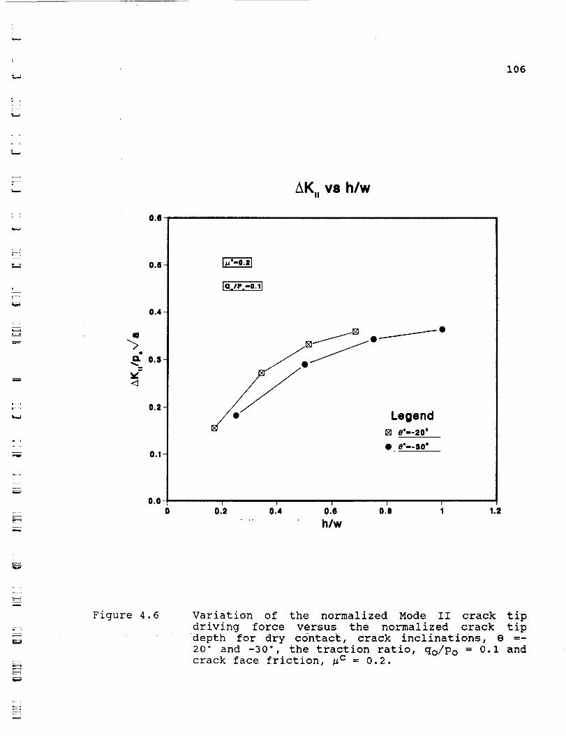
106

E

i :

:==

FL: ,:

ram.

--=mmr

m

0.e

0.6

0.4-

_. 0.3-=

0.2 -

0.1 -

0.0 -

0

AK,,vs hlw

Legend

[] 0"'-20'

• 8"--$0'

I I I I I

0.2 0.4 O.e 0.8 1

+ h/w1.2

=

I

Figure 4.6

+




20 ° and -30 ° , the traction ratio, qo/Po = 0.i and

crack face friction, _c = 0.2.

_:_

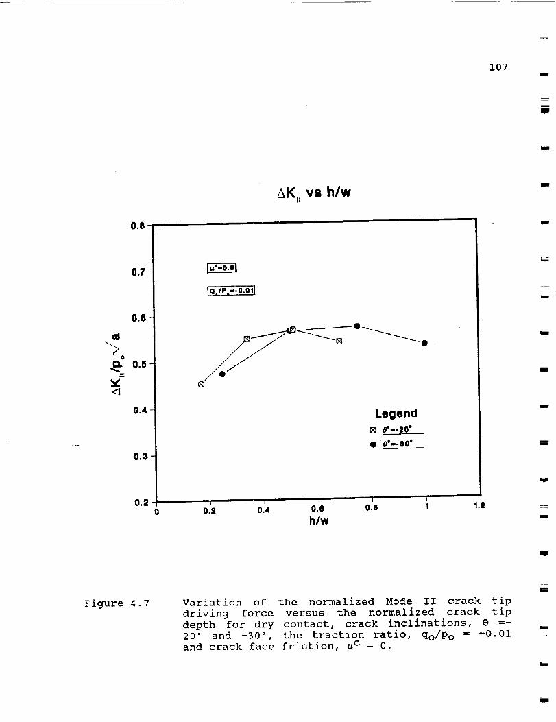
107i

i

m

0.8

0.7

0.6 -

@

O.5-

0.4

0.8

0.20

AK,, vs h/w

Legend

W"20'

• e'--$O'

"0

0.2 0.4 0.8 0.8 1

h/w

1.2

Ill

I

m

W

I

IBm

m

R

Im

Figure 4.7Variation of the normalized Mode II crack tip



20 ° and -30 ° , the traction ratio, qo/Po = -0.01and crack face friction, _c = O.

i

m

108

0.8

0.7-

0.6-

0.6-

0.4 -

0.3-

0.20

v8 h/w

Legend

[] e'--20'

I e'--$0'

I I I I |

0.2 0.4 0.6 0.8 1

.... _ h/w

1.1

G _




20" and -30", the traction ratio, qo/Po = -0.05

and crack face friction, _c = O.

.----,

i

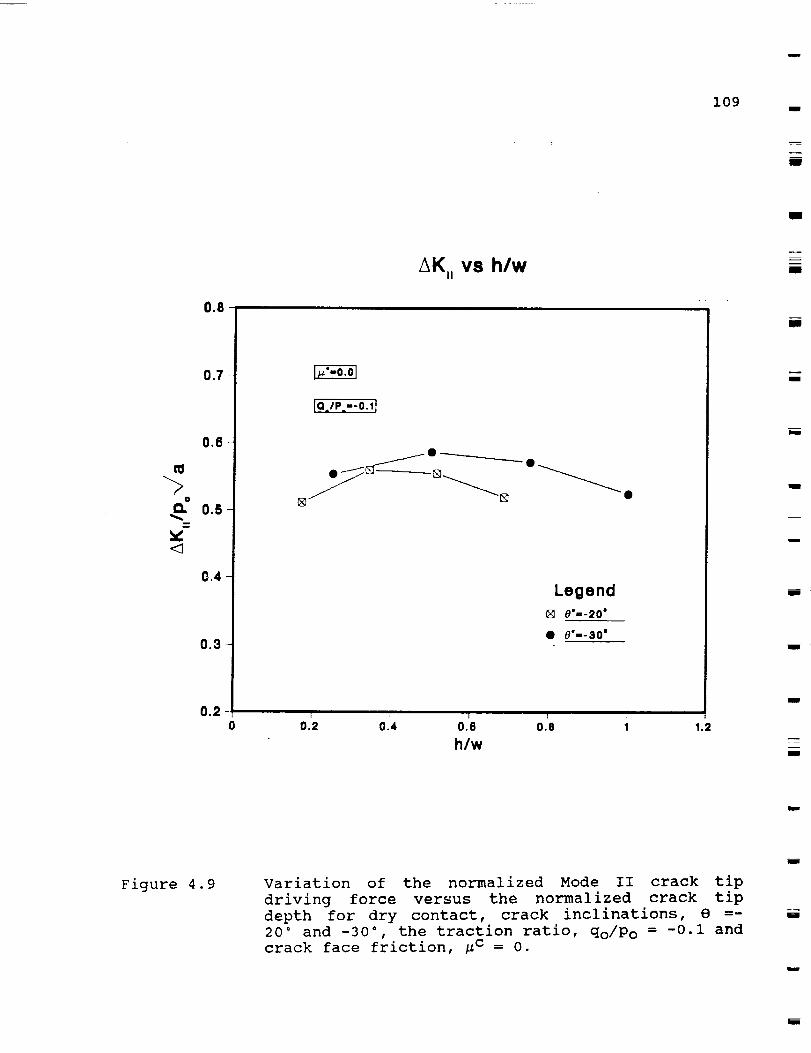
109mm

m

mE

0.8

0,7

0.8

0

Q. 0.5

0.4

0.3

0.2o

AK,,vs hlw

_e_ e

Legend

0.'2 0._4 0._8 0._8

h/w1.2

am

BE

m

mImm

U

u

role

I




20 = and -30 ° , the traction ratio, qo/Po = -0.I and

crack face friction, _c = O.

m

M

J

i

ii0

=

0.6

0.5

0.4

Q

0.$

v

0.2

0.1

0.0

" AK,, vs h/w

Legend(_ 8"'-20'

• e"-SO"

' 0 .'4 0 .'8 ' '0.2 O.O 1 1.2

h/w



depth for dry contact, crack inclinations, 8 =

-20 ° and -30", the traction ratio, qo/Po = -0.01and crack face friction, _c = 0.2.

IIi1

ll

Ill

0.6

0.5

0.4

m

o

D. 0.$

/

/O.2 /

/

//

o.1-

0.0-0

AK,, vs hlw

[QJP.--O.081

/

Legend[] 0""-20'

• 8"'-$0'

0 .'2 ' 0 .'8 ' '0.4 0.e 1

hlw

e

1.2

mm

mi

mE

w

Ill

I

IBm

m




20 ° and -30 ° , the traction ratio, qo/Po = -0.05

and crack face friction, _c = 0.2.

ll

III

E:112

1

i

L •

0.6

0.5

0.4

0

Q. 0.3-

0.2

0.1

0.00

i

AK. vs h/w

®___[]'

e_ e

Legend0"-20'

"• 6"'-$0'

I I I I I

0.2 0.4 0.6 0.8 1 1.2

h/w

w

i




20 ° and -30 ° , the traction ratio, qo/Po = -0.i andcrack face friction, _c = 0.2.

i

113

U

mm

O

2

1.5

0.5-

0

-0.5

K,, AND K, vs x/w

IQJP.-0.11

//

/F

\\

Legend

K.

I I I I • I

-8 -2 -1 0 1 2 $ 4 6

x/w

m

I

i

U

m

roll

from

IBB

u

I

w

Figure 4.13 Variation of the normalized, Mode I and Mode II

stress intensity factor versus the normalized

distance between the contact and the crack mouth

for lubricated contact, a relative crack length,

a/w = 0.5, crack inclinations 8 = -30 ° , the

traction ratio, qo/Po = 0.i, and crack face

_c 0.friction, =

lm

mum

l

m

114

z

w

B

m

oQ.

.

1.5-

0.5-

-0.5

K. AND K, vs x/w

-$

I,'--8o.o'l

lagi,.-o.ll

Legend

Kit

'-h

// \/ \

J

-2 -1 0 1 2 8 4 6

X/W

Figure 4.14 Variation of the normalized, Mode I and Mode IIstress intensity factor versus the normalized


for lubricated contact, a relative crack length,a/w = 0.5, crack inclinations 8 = -30 ° the

traction ratio, qo/Po = 0.i, and crack facefriction, _c = 0.2.

115mm

im

1.3

AK,, vs h/wam

I

1.1

0.5-

0.3

0

m 0.9

0

¢,1

<1 0.7

Legend

[] 0"--20'

• , _e'--8o"

,I I I ! I0 0.4 0,8 0.$ 1 1.2

h/w

i

i

m

m

ida

if

lid

i

lip



depth for lubricated contact, crack inclinations,

8 = -20 ° and -30 ° , the traction ratio, qo/Po =

0.01 and crack face friction, _c = O.

i

m

I

i

w

116

r_

m

i

r_

R

w

= :

1.3

1.1-

O.g-

0

Q.

<_ 0.7-

0.5-

Figure 4.16

AK,,vs hlw

[] []-,

Legend

[] 0"--20'

• •'--SO*

Io./e.-o.osI

I 1 I I0 2 0.4 0.8 0.8 1 1.2

h/w




S = -20 ° and -30 ° , the traction ratio, qo/Po =

0.05 and crack face friction, _c = 0.

117I

I

I

1.3

1.1

m 0.9

O

¢,j

•<_ 0.7

0.5

0.3

AK,,vs hlw

• Legend[] 8"--20

• e'--$O'

Io./P.-O.ll

0

iiI I I I I

0.2 0,4 0.6 0,8 1 1.2

h/w

I

I

=i

mE,'

i

mqpz




8 = -20 ° and -30 ° , the traction ratio, qo/Po = 0.i

and crack face friction, _c = O.

i

I

i

118

T

D

l

v-

[-:

: Lw

1.3

1.1-

m 0.9-

0

<:I 0.7-

0.5-

0.30

AK,, vs hlw

la.iP.-O.OlI

Legend[] 0"--20'

• O"--SO'

' 0.'8 ' '0,2 _: 0.4 0.8 1

: h/w

1.2

--m




S = -20 ° and -30", the traction ratio, qo/Po =

_c 0.2.0.01 and crack face friction, =

119

I

1.3

1.1

(0 0.9

o

Q.

<_ 0.7

0.5

0.3

AK,, vs hlw

Legend[] e'--20'

• 0"--$0'

I I I t I

0.2 0.4 0.6 0.$ 1

h/w

1.2

U

m

u

mmm

ma

U

U




8 = -20 ° and -30 ° , the traction ratio, qo/Po =

0.05 and crack face friction, _c = 0.2.

m

u

J

u

-w-

120

L

i

=

B

Km

1.3

1.1-

a:l 0.9

0

<:1 0.7--

0.5 -

AK,, vs h/w

Legend

IQ./P.-o.ll

' ' 0.'8 0._8 '0.2 0.4 " 1 1.2

hlw

!

m

w




S = -20 ° and -30 ° , the traction ratio, qo/Po = 0.I

and crack face friction, _c = 0.2.

w

121

z

I

m

I

o

m

3.5

_

2.5

1.5

AK, vs h/w

Legend

Io.IP.--O.ll _•

i " 'J I t I

0.2 0.4 0.6 0.8 I

hlw

mQlm

zI

I

I

11m

I

im

llm

[]

am

zI

Figure 4.21 Variation of the normalized Mode I crack tip



8 = -20 ° and -30 ° . The Mode I values are

independent of the traction ratio and the crack

face friction-

I

I

I

I

122

t--

_s_

=

=

m

0

.

1.5-

0.5

0

-O.B

K,, AND K, vs x/w

18"----.o'1

laJP.--O.ll

////

/!

TI ..... /

-tJ

Legend

K.

K_,

\\\\

I I ! I I I

-8 -2 -1 0 1 2 $ 4 5

x/w

v_





a/w = 0.5, crack inclinations 8 = -20 ° , the

traction ratio, qo/Po = -0.i, and crack facefriction, _c = O.

123

J

m

1.5

@

0.5-

_

Io'--,o.o'J

JQJP.--O,lJ

K,, AND K, v8 x/w

/,",_///////

\

Legend

Kal

I I I I I I

-2 -_ 0 1 2 8 4 II

x/w

J

mm

m

mmm

l

m

w

m




for lubricated contact, a relative crack length,a/w = 0.5, crack inclinations 8 = -30 ° , the

traction ratio, qo/Po = -0.i, and crack facefriction, _c = 0.2.

mm

J

w

I

124

m

L

W

=_

L--"

al

.

1.6

0.5 ¸

-

K. AND K, v8 x/w

Je'--:to.o'J

IQ.IP.--0.1]

/,",_///t///

\\

\

&,.

Legend

K.

K,

-8 -2 -1 0 1 2 8 4 6

X/W


._-...... stress intensity factor versus the normalized


...... for_lubric_tgd 99Dtaqt, a relative crack length,

a/w = 0.5, crack inclinations 8 = -30 °, the

traction ratio, qo/Po = -0.i, and crack facefriction, _c = O.

125I

I

i

i

2

1.5

O

v0.5

o

-0.5-8

IQ./P.--0.11

K,,AND K, vs x/w

///

/

F

, /

Legend

K.

K_

\\\\

I I " l I ! I

-I -I 0 1 2 $ 4

xlw

i

II

i-

"iI

*mm

_r

z

m

i

I





a/w = 0.5, crack inclinations G = -30 ° , the

traction ratio, qo/Po = - 0.i, and crack face

friction, _c = 0.2.

in

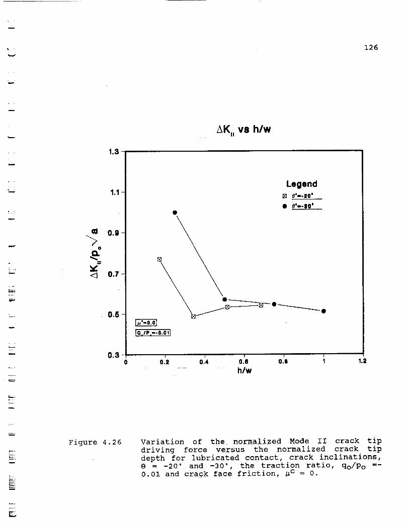
w

126

u

w

o •

w

z

A

L

m

1.3

1.1-

m 0.9-

o

Q.

<I 0.7-

0.5 -

AK,,vs hlw

Legend

0",--|0'

• P"'$O'O

la./p.--o.o_l

' ' 0 .'e 0 .'$ '0.2 0.4 1

h/w

1.2




S = -20 ° and -30 ° , the traction ratio, qo/Po =-

0.01 and cragk face friction, _c = o.

127

w

mm

1.3

1.1

c_ o.g

@

Q.

._ 0.7

0.5

0.3

AK,, vs h/w

0

Legend

e_ e

la./p.-.o.os]

I I 1 I I

0.2 0.4 0.8 0.O 1

h/w

1.2

m

IBm

Im

m

qlm

'm

imF

J

mm

lib




e ='-20 ° and -30 °, the traction ratio, qo/Po =-

0.05 and crack face friction, _c = O.

u

g

128

.

m

1.3

.1 -

0.9-

o

_ 0.7-

0.5_

AK,, vs h/w

Legend[] e'--20'

• 6"--$0'

I I l I I

0.2 0.4 o.e o.e 1.... h/w

1.2

z

w

m

_=

__ +w

w




8 = -20 ° and -30 ° , the traction ratio, qo/Po =-

0.i and crack face friction, _c = 0.

129 ,j

m

m

R

1.3

1.1

CO 0.9

oa.

<1 0.7

0.5

0.3

AK,, vs h/w

0

Icajp.--o.o,;

Legend

1 i i

O: , ., i ,2 0.4 0 (! 0.8 1 1.2

h/w

I

iwm

/

m

ira,

I

ill

qua,




8 = -20 ° and -30 ° , the traction ratio, qo/Po =-0.01 and crack face friction, #c = 0.2.

mm

% 130

1.3

1.1-

¢0 0.9-

0

a,

<:_ 0.7-

0.5-

0.30

AK,, vs h/w

*_ e

la./e.--o.o61

Legend[] 8"-RO'

• 8"'-SO'

' 0 .'4 0 .'6 ' '0.2 0.8 1 1.2

............ h/w

= ,

=--




S = -20 ° and -30 °, the traction ratio, qo/Po =-

0.05 and crack face friction, _c = 0.2.

z :

131D

mm

l

1.3

AK,, vs hlwImm

Imm

1.1

¢0 O.g

0

<:I 0.7-

0.5 -

0.30

Legend

e'--20*

• e'--80*

I I I I I

0.2 0.4 0.8 0.8 1

h/w

1.2

W

"am

Imm

m




8 = -20 ° and -30 ° , the traction ratio, qo/Po =-

0.i and crack face friction, #c = 0.2.

D

m

m

I

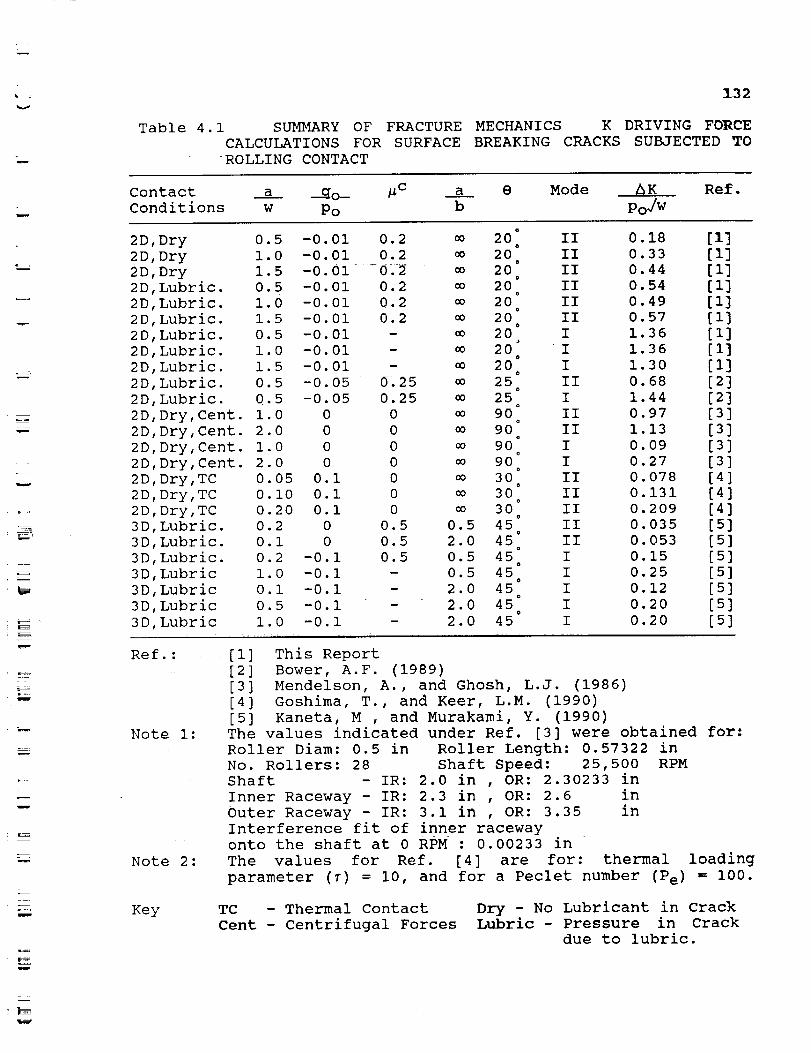
1.32

Table 4.1 SUMMARY OF FRACTURE MECHANICS K DRIVING FORCE

CALCULATIONS FOR SURFACE BREAKING CRACKS SUBJECTED TO

_ROLLING CONTACT

Contact a --qo-- _c a 8 Mode _K Ref.

Conditions w Po b PoJW

L_

2D, Dry

2D, Dry

2D, Dry

2D, Lubrlc.

2D, Lubric.

2D, Lubrlc.

2D, Lubric.

2D, Lubrlc.

2D, Lubrlc.

2D, Lubrlc.

2D, Lubrlc.

0.5 -0.01 0.2

1.0 -0.01 0.2

1.5 -0.01 0.2

0.5 -0.01 0.2

1.0 -0.01 0.2

1.5 -0.01 0.2

0.5 -0.01 -

1.0 -0.01 -

1.5 -0.01 -

0.5 -0.05 0.25

0.5 -0.05 0.25

2D,Dry,Cent. 1.0

2D,Dry,Cent. 2.0

2D,Dry,Cent. 1.0

2D,Dry,Cent. 2.0

2D,Dry,TC

2D,Dry,TC

2D,Dry,TC

3D,Lubric.

3D,Lubrlc.

3D,Lubric.

3D,Lubric

3D,Lubric

3D,Lubric

3D,Lubric

0 0

0 0

0 0

0 0

0.05 0.i 0

0.i0 0.i 0

0.20 0.i 0

0.2 0 0.5

0.i 0 0.5

0.2 -0.i 0.5

1.0 -0.i

0.I -0.i

0.5 -0.1

1.0 -0.i

20[ II 0.18 [I]

20 II 0.33 [I]e

20° II 0.44 [i]

20° II 0.54 [i]20 II 0.49 [i]

°

20° II 0.57 [I]20 I 1.36 [i]

20° I i. 36 [I]

20° I 1.30 [I]

25° II 0.68 [2]

25 I 1.44 [2]o

900 II 0.97 [3]

90 II 1.13 [3]o

90 I 0.09 [3]e

90 I 0.27 [3]o

30° II 0.078 [4]

30° II 0.131 [4]30 II 0.209 [4]

e

0.5 45 II 0.035 [5]o

2.0 45 II 0.053 [5]o

0.5 45° I 0.15 [5]

0.5 45° i 0.25 [5]2.0 45 I 0.12 [5]

o

2.0 45 I 0.20 [5]0

2.0 45 I 0.20 [5]

L ....

w

L--==w

.==

w

Ref.:

Note i:

Note 2:

Key

[i] This Report

[2] Bower, A.F. (1989)

[3] Mendelson, A., and Ghosh, L.J. (1986)

[4] Goshima, T., and Keer, L.M. (1990)

[5] Kaneta, M , and Murakami, Y. (1990)

The values indicated under Ref. [3] were obtained for:

Roller Diam: 0.5 in Roller Length: 0.57322 in

No. Rollers: 28 Shaft Speed: 25,500 RPM

Shaft - IR: 2.0 in , OR: 2.30233 in

Inner Raceway - IR: 2.3 in , OR: 2.6 in

Outer Raceway - IR: 3 1 in , OR: 3.35 in

Interference fit of inner raceway

onto the shaft at 0 RPM : 0.00233 in

The values for Ref. [4] are for: thermal loading

parameter ([) = i0, and for a Peclet number (Pe) = I00.

TC - Thermal Contact

Cent - Centrifugal Forces

Dry - No Lubricant in CrackLubric - Pressure in Crack

due to lubric.

133

cracks, the relation between the normalized driving force andcrack length is parabolic 14 (O'Reagan et al., 1985) and thisfacilitates interpolations. However, this is not the case forthe surface breaking cracks examined here and any interpolationsto small crack lengths must be done with caution even though thedriving force for vanishingly small cracks does approach zero.

The results in Figure 4.32 reveal that pressure from fluidin the crack cavity, centrifugal stresses and thermal stresseseach add significantly to the _K-driving force, particularly forrelatively short cracks, a/w < 0.i. However, they are notnecessarily additive because they do not peak at the Samerelative contact location. Fluid in the crack cavity isespecially potent since it generates Mode I values that are evenlarger than the Mode II values. The compilation suggests thatall but the smallest, surface breaking, lubricated cracks maygrow in Mode I. It is also evident that the driving forcesgenerated by 3 dimensional cracks are =20% of the values obtainedfor 2-dimensional cracks. Since the real spall nuclei are 3-di-mensional (see Section 5.4), the 3-D results of Kaneta andMurakami (1990) appear to be most relevant for estimating growthon the 3-ball-rod testing machine. The following expressionsapproximate the variation of the driving force with crack lengthfor this case:

AK I = A (a/w) B P0 Jw .............. (4.1)

where A =2.3 and B = 0.3.

4.5 Evaluation of Threshold Crack Sizes.

Insight into the significance of the driving force values

can be obtained by installing a separate set of curves describing

the conditions at the threshold for growth. By inserting speci-

fic values of the peak contact pressure, P0, and the threshold

value of _K, curves describing the driving force requirements

for different threshold flaw sizes can be generated. These

curves are overlayed in Figures 4.33-4.34 on the results of the

driving force analyses in Figure 4.32 for 2 contact pressures and

2 estimates of the threshold, _Ktbr_shold" The coincidence ofthe results from a particular urlvlng force source and the

threshold curves define the critical crack size for growth in

each case. Cracks smaller than the threshold would either not be

expected to grow, or to enlarge much more slowly as part of the

crack nucleation process. Since crack nucleation is assisted by

hard particles and inclusions, the critical flaw size can be

viewed as a rough measure of the tolerable inclusion size.

14 _K/P0/a = A or _d</(P0/W ) = A /(a/w) where A is a constant.

W

J

n

m

mm

I

u

J

E,_

g

n

g

m

I

U

w

134

===

1.6'

1.2"

O

h£o.8-

0.4-

0-

o

[]

[][]

[]

0.6

AK,,/poCJ '= vs (a/u)

[][]

@

[][]

¢

8 [][]

1 1.8 2.8(a/_)

1Legend

5_ K,.2D.L

K..2D.D

K,,.2D.L

• K,,,2D,L

:_] K,.2D,L

K,,.2D.D.C

K,.2D,D,L

-7 K,,,2D.D.TC

• K,,,3D.L

K,.3D.L

Figure 4.32 Normalized, Mode I and Mode II stress intensity

factor ranges reported by different investigators

for different sources of the cyclic crack growth

driving force and for different relative crack

lengths. Details can be found in Table 4.l.The



lubricated, C - centrifugal stress and T - thermal

stress.

135 m

AK,,/po ''= vs

[][]

Po=2400 MPa AKTH----_2MPa.m V2

Po=3600 MPa'_KTH=3 MPa.m v2

[]

[]

@

(e/_)

[]

Legend

KI.2D.L

K,,.2D.D

K..2D.L

• K..2D.L

K,.2D,L

K..2D.D.C

Kj.2D,D.L

-7 K..2D.D.TC

K.,3D.L

K,.3D.L

[]

m

'BIB

J

m

m

IIIBB

m

mW

M

IB

lib

Figure 4.33 Curves describing the conditions at the threshold

for cyclic crack growth for either a Hertzian

contact pressure, Po = 2.4 GPa and a _KTHRESH = 2

MPa or Po = 3.6 GPa and a _KTHRESH = 3 MPa.

These are overlayed on data points representing

the normalized, Mode I and Mode II stress

intensity factor ranges reported for different

sources of the cyclic crack growth driving force

in Figure 4.32. The coincidence defines the

conditions for the onset of crack growth in each

case. The following abbreviations are used: 2D-

2-dimensional, 3D - 3-dimensional, D - dry, L-

lubricated, C - centrifugal stress and T - thermal

stress.

J

i

mmu

=

J

136

m

E

w

= -

, AK,,/po_ v2 vs (a/_)

6

//o

[]

o 0.5 I(a/w)

AKTH-_5 MPa.m _/2

Po=2400 lvIPa

[]

!Legend

KI.2D.L

K,,.2D.D

_1 K..2D.L

II K..2D.L

K,.2D.L

_t K..2D.D.C

KI.2D.D.L

K,,,2D,D,TC

I) K,,,3D,L

K,.3D,L

[]

a = 30 #m

1,5 2 2.5

=--

Figure 4.34 Curves describing the conditions at the threshold

for cyclic crack growth for a Hertzian contact

pressure, Po = 2.4 GPa and a _KTHRESH = 5 MPa.

These are overlayed on data points representing

the normalized, Mode I and Mode II stress

intensity factor ranges reported for different

sources of the cyclic crack growth driving forcein Figure 4.32. The coincidence defines the

conditions for the onset of crack growth in each

case. The following abbreviations are used: 2D-

2-dimensional, 3D - 3-dimensional, D - dry, L-

lubricated, C - centrifugal stress and T - thermalstress.

137

surfaces, a Hertzian pressure of Po = 2.4 GPa and a K_-threshold= 5 MPa, 3-dimensional, surface breaking cracks (and Inclusions)with dimensions, a = i0 _m can be tolerated in a perfectly smoothwell lubricated bearing. The centrifugal stress contributionappears to be negligible. The defect tolerance will be reducedsomewhat by thermal stresses arising from loss of lubrication andsliding. The a = i0 _m defect dimension is larger than theinclusions normally encountered in bearing grade 440C. Consis-tent With this, the contact lives of 440C samples which contain=i0 _m- surface breaking cracks exceed N = 6.10 s contacts whenthey are tested at Po = 2.4 GPa in the 3-ball-rod tester. Thecracks do not grow under these conditions. At higher contactpressures the same a = i0 _m surface cracks do grow into spallsand reduce the contact life dramatically (see Section 5.4).

4.6 Conclusions

Efforts have been made to extend the Bower treatment of 2-dimensional, surface breaking cracks with fluid in the crackcavity to smaller relative crack lengths, but the Bower algorithmproved unstable for a/w < 0.5. In the range 0.5 < a/w < 1.5, thevalues of the normalized driving force, K/P0Ja decrease with therelative crack length, a/w, for lubricated contact, but increasefor dry contact

A compilation of K-driving force values of surfacebreaking cracks has been assembled. This reveals that fluid inthe crack cavity, centrifugal stresses, and thermal stresses addsignificantly to the crack driving force, particularly forrelatively short cracks, a/w < 0.I. Fluid in the crack cavity isespecially potent, producing relatively large Mode I drivingforce values. The driving forces generated by 3-dimensionalcracks are = 20% of the values calculated for 2-dimensionalcracks.

As a result of the modest driving force generated by small,3-dimensional cracks, surface cracks as large as a = i0 _m wouldnot be expected to grow in idealized smooth, well lubricatedbearings with a Mode I, KTHR_SH = 5 MPa subjected to a HertzianPressure, Po = 2.4 GPa. Thls is consistent with experimentalresults described in Section 5.4.

r_

g

U

l

m

Im

m

W

lwmm

g

m

w

z

L_,

w

-==

138

5. ROLLING CONTACT FAILURE

5.1 Background

The life of an element subjected to rolling contact loading

is limited by the premature spalling and heavy wear of the

bearing races and balls. The spalls are mainly surface

initiated, proceeding in both balls and races, and propagate

inward with distinctive geometric features.

The spalling process is driven by the surface frictional

tractions, Soda (1981), and by the stationary pressure spikes

originated at surface irregularities, Hamrock (1990). Additional

complications may be caused by: a) the presence of subsurface

secondary particles or inclusions, which may lead to subsurface

initiated cracks, b) strain induced phase transformations, i.e.

retained austenite decomposition, carbide dissolution, c)

lubrication conditions at the surface, or d) thermally induced

stress fluctuations (as treated in Section 3.5), which eventually

contribute to the Modes I and II driving forces (as indicated in

Section 4.4).

This section describes experiments conducted on 440C bearing

steel in order to gain a better understanding of the mechanisms

leading to spall failure under different conditions.

5.2 Experimental Materials and Procedures

The rolling experiments were carried out on the 3-ball-rod

rolling contact fatigue tester developed by the ball and roller

bearing group at Federal-Mogul, and furnished by NTN Bower. The

design and operation of the tester machine has been described by

Glover (1982).

The test material is AISI 440C, martensitic stainless steel,

heat treated to a hardness of 59-61 HRc. The test samples were

subjected to the following heat treatment:

a) Austenitized at 1930±30 _F for 1 hour at temperature.

b) Hardened by quenching in liquid nitrogen.

c) Tempered one hour (minimum) at 325±25 gF.

d) Cooled in air to 70±10 QF.

e) Cold soaked in liquid nitrogen for 30 minutes.

f) Tempered for 1 hour at 325±25 gF.

The geometry of the samples is shown in Figure 5.1. The test

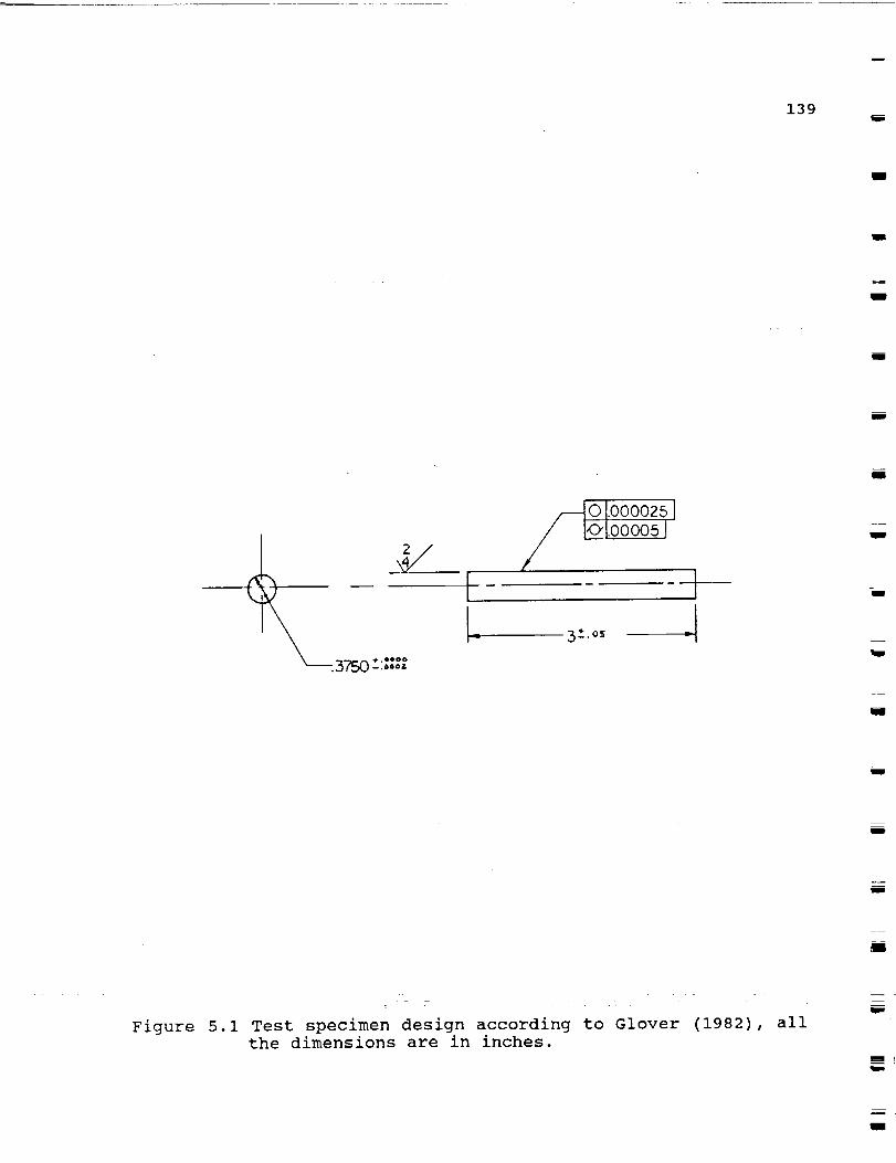
139mum

m

J

l

U

I 2/J/

L3750t::::_

///--_o I.oooo_5I

_1.oooo51

J

rW

g

mJ

m

m

m

Figure 5.1 Test specimen design according to Glover (1982), allthe dimensions are in inches.

mmW

u

m

L

L__

_ _

r

w

_m

m

140

samples were ground to a surface finish of 6.5 AA (0.165 _m),

with a roundness of 1.27-1.54 _m (a more detailed study of the

surface finish is included in Figure 5.2). Each rod can be used

to perform up to 8 individual tests.

The balls used in the RCF tester are made of AISI 52100

bearing grade steel. Two differen_t sets of balls were used during

the tests. The first set consisted of balls with smooth surface,

i.e. 0.34 AA (8.6xi0 -3 _m), and the second set consisted of balls

which are abrasive blasted to increase the surface roughness,

i.e. 4.28 AA (0.ii _m). A more detailed surface analysis of both

types of balls can be seen in Figures 5.3a and b. The chemical

compositions for both the 440C and the 52100 steels are shown in

Table 5.1.

5.2.1 Rollinq Contact Testinq: A total of 21 individual tests

(see Table 5.2), distributed among three specimens wereconducted. After each test the balls were replaced to insure

uniform testing conditions. Exxon grade 2380 turbine oil was used

as a lubricant in all the tests. The oil was applied by drip feed

at a rate of i0 drops per minute. A spring load of 253.6 N was

used in all the tests. The peak Hertzian pressure was calculated

to be equal to 5.4 GPa.

Six tests were conducted under similar conditions to

determine the amount of scatter in the results (Test Series I).

An attempt was also made to vary the content of retained

austenite in the specimens by soaking in liquid nitrogen for

different lengths of time; a total of i0 tests were devoted to

this purpose (Test Series 2). Three more tests were conducted

with smooth balls in order to register any differences in the

failure life, location and size of spalls, or the surface

appearance after the test (Test Series 3). Two additional tests

were conducted using rough balls in order to study the contacting

surface (Test Series 4). The tests were interrupted after a short

time after starting to examine and photograph the surface under

the scanning electron microscope. After examination, the

specimens were inserted back into the RCF tester. The tests were

continued until spalling failure occurred.

The fatigue test results summarized in Table 5.2 have been

analyzed using the two-parameter Weibull statistics. The Weibull

estimates for the two cases are summarized in Tables 5.3 and 5.4,

respectively. Graphical representation of the test data is

illustrated in Figure 5.4. The procedure adopted to obtain the

Weibull parameters is similar to the graphical method described

by Lipson and Sheth (1973). A computer program was written to

evaluate the LI0 and L50, as well as the characteristic lives,

and the upper and lower bounds for the 75% confidence levels, by

using a binomial distribution method.

h

w

Table 5.1 Composition of 440C and 52100

141I

Steel C Mn Si Cr Ni Mo Cu A1 P Si

440C 1.05 .44 .44

52100 1.02 .34 .32

17.11 .i0 .48 .04 .02 <.022 <.001

1.45 0.13 .05 .16 --- <.09 <.014

g

i

Balance Fe. q

L__

i

II

I

I

I

m

I

142

i ;

+ .

m

_=_

F] - Anal4si5F2 - CraphF3 - DumpF4 - Exp_dF5 - Exc:ude

F6 - Z__anQP

-32.48 uin-

FI - Analysis

I bode I Cut Off fFilter Referer,ce I l,nore

IRouc,,_ssi 83_ioIIsoiSTR_tC,_+_.[ RCF P_D 44_-{ GROUND

iI+ Vi .+,

i

I57.499 ain )l

Peak lo UalIe4 : 56.75 uin

I Mode ] Cut 0?£ =ilterI Reference ignore

ROUGHNESS .e38 in ISO I STR_IGHI BRCF ROD 44_-C GROUHD++_.:?! : :

RII =

Rpa =R+ =Rtt =Rt? :Rt3 =Rt4 :Rt5 :

45.57 uJn Lo = 157.499 min Ra = 6.47 uin

28.62 uin Rp : 24.28 uin Rq : 8.14 uin56.58 uin Rv : 3_.48 uin Rsk = -.356.58 uin Rt : 56.75 uin Rku : 3.455162 uin Delq : 2.22 _eg39.22 uin SLOPE = .ii Deg Lamq = 1.322 min36.85 uin S = 625.18 u/n39.66 uin Sm : 1.227 Iin

: R3Z = 34.54 uin

E34 : 43.39 uin

Figure 5.2

A_ORIGINAL P_E IS

OF POOR QUALITY

Surface roughness of 440-C RCF test sample. (a)

Shows the profilometer trace, with a peak-to-

valley value of 56.75 #in, (b) shows an analysisof the profile, worth noticing the surface finish

of 6.5 _in, and (c) the roundness analysis

indicates a good value, i.e. 50-60 #in.

143

=

F] _' Analus_sF2 - GraphF3 - DumpF4 - ExpandF5 - ExcludeF6 - Z.R_nge

i Mooe i Cut O£F IFilter Re_erencel Ignore)

ROUGHNE)S I .83_ in ) )SO CONUEY L 8 _ JRCF M_TER' BALL l] LOT 11238 _v__

,%

-49.38 uin( 163.29_ kin )I

Peak To LiaI!eu.:- 17 67 uir,

FI - AnalgsisMode " I Cu_ O£f IFiIter)Reference)IQnorel

ROUGHHESS [ 838 in I ISO / COHUEX_--A'STSTERBALL #] LOT #1238

m

mmm

mmm

,row

F,'t _m --

F:ph =R_. =Rtl =R12 =Rt3 =Ri4 =Rt5 =

48.82 uin24 29 uir,88 78 u)n23 93 uin27 18 uin42 57 uin29 71 uin88 78 uin

Lo = 16?.293 _inRp = 48.34 uinRv = 49.38 uinRt = 97.63 uin

RADIUS = .25826 in)iameter = .58851 it,

Ra = 4.18 ulnRq = 6.11 uinRsk : 1.4Rl:u = 16.4

Delq = 2181 legLamq = 1.897 minS : 582.37 uinSm = I._22 minR3: = 24.58 uin

R3y : 38.82 uin

l

i

z --

m

Figure 5.3.a Surface roughness analysis of a 52100 RCF ball.

The ball has been grit (sand) blasted to a surface

finish of 4.18 _in, for a peak-to-valley of 97.63

_in.

ORIGINAL PAGE iSOF POOR QUALITY

Nil

144

FI - ¢_na}g._isF_'- GraphF3 - DumpF4 - ExpandF5 - Excluoe

1.49 uir,-

-4.96 uir,-

FI Anal_sis

Mc,_e I Cut Of_ iFil%er i Re_erence !9nor.e

IROUGHNE% j .B_ inl ISO I COPVEX. I _ ;;RCF NEW BALL BEFORE SANDBLRSTING PROCESS

164 5_9 min

Peal:To Ua]leq = 6 46 uir,

l,,_.ode )Cut Of.c Fil,er Reference I_ore I

ROuuI_REo._I .83B .inl ISO I CONUEX i 8 ;; I

_I RCF NE_ BALL BEFOFcESAHI_BLRST]HGPROCESS i

Rt2 =R13 =R_4 :R15 =

2 73 uin82 uin

5 54 uinl 79 uin2 45 uinI 77 uir,5 54 uin2 ll uin

Lo = 164.569 wit:R_. = 1.49 uinRv = 4.96 uinRi = 646 uin

RADIUS = ._u@:@ in)iame;er : .5BMl in

Ra : 74 uir:Rq : .47 uinRsk : -.BRku : 15.2_e!q : .12 _egLamq : 1.359 minS = 556.87 uin

Si : 1.312 minR3z : 1.68 uinR3g = 1.98 uin

Figure 5.3.b

ORIGINAL PAGE IS

OF POOR QUALITY

Surface roughness analysis of a 52100 RCF ball.

The ball has been lapped to a surface finish of

0.34 #in, for a peak-to-valley of 6.34 #in.

145

Table 5.2 Result of Rollinq Tests

Test Series i: Study of the contacting surfaces and scatter in

the experimental data (combined with Test Series 3

for the statistical analysis shown in Table 5.3)

Test Specimen Track Machine Hours Ball Hours to Stress

# ID # Head in LN 2 Lot 15 Failure Cyclesxl06

1 A1 L1 1 0 R 22.0 11.33

2 A2 L1 1 0 R 10.4 5.36

3 A2 L3 1 0 R 6.4 3.30

4 A2 L5 1 0 R 2.4 1.24

5 A2 L7 1 0 R 2.4 1.24

6 A2 L9 1 0 R 10.4 5.36

Test Series 2: Retained austenite study.

7 A1 L3 1 1 R 27.8 14.32

8 A1 L5 1 2 R 7.5 3.86

9 A1 L6 2 3 R 22.1 11.38

i0 A1 L7 1 3 R 15.2 7.82

ii A1 L8 2 3 R 14.2 7.31

12 A2 L2 2 2 R 3.9 2.00

13 A2 L4 2 2 R 6.4 3.30

14 A2 L6 2 2 R 1.0 0.52

15 A2 L8 2 2 R 16.6 8.54

16 A2 LI0 2 2 R 3.4 1.75

Test Series 3: Initial study of ball roughness effect.

17 A1 L2 2 3 S 30.4 15.65

18 A1 L9 1 3 S 14 .0 7.20

19 A1 LI0 2 3 S 63.6 32.75

Test Series 4: Study of the contacting surfaces and scatter in

the experimental data (combined with Test Series 3

for the statistical analysis shown in Table 5.3)

20 A6 L2 2 0 R 19.6 I0.09

21 A6 L3 2 0 R 5.3 2 .7

J

mmm

i

g

i

m

w

m

l

imw

z_

l

mm

.=

15 R=Rough Lot, S=Smooth Lot

m

w

U

_-n=,

E

146

Table 5.3 Two-Parameter Weibull Estimate for Case 1

Study of the contacting surfaces and scatter in the experimental

data are combined here. The results shown under Test Series 1 and

4 in Table 5.2

Item Cycles Median Ranks

1 0.124xi07 0.08300

2 0.124xi07 0.20210

3 0.273xi07 0.32130

4 0.330xi07 0.44040

5 0.536xi07 0.55960

6 0.536xi07 0.67870

7 0.101xl08 0.79790

8 0.113x108 0.91700

Slope = 1.24469 LI0 = 0.94748xi06

Intercept = -19.37923 L50 = 0.43041xi07

Characteristic Life = 0.57778xi07

Correlation = 0.9633787

Table 5.4 Two-Parameter Weibull Estimate for Case 2

Study of the effect of retained austenite in the fatigue life

using the results shown as Test Series 2 in Table 5.2.


1 0.520xi06 0.10910

2 0.175xi07 0.26550

3 0.200x107 0.42180

4 0.330xi07 0.57820

5 0.386xi07 0.73450

6 0.854xi07 0.89090

Slope = 1.11034

Intercept = -16.81940

LI0 = 0.49944xi06

L50 = 0.27247xi07

Characteristic Life = 0.37904xi07


147 mm

mm

i

@0

0 GO

F

C ,0

F D

A F2@

I

L %

U

R

E

99

W

90 --

70 --

50 --

30

10

5 ---

2

10000

WEIBULL ESTIMATE FOR VALUES IN TABLES 5.3 AND 5.4

rr r!ll

o--: : :

i

! L-I,

!fl

Irlii i r i

r I

__L

___ L

/

/

//

// /

y

/ ....

• //

/

--/ .... i

m

100000 1000000 &E_07 IE_@@

LIFE (STRESS CYCLES)

L_

L% 75

U% 75

o CASE t

L% 75

U% 75

CASE 2

m

m

mi

i

m

lira,

m

Figure 5.4 Weibull plot for the RCF test results presented in

Tables 5.3 and 5.4, peak pressure, Po=5.4 GPa.

Case 1 (circles) represent the statistical

analysis of the results of the Test Series 1 and 4

from Tables 5.2. Case 2 (triangles) are the

results of the study of the influence of retained

austenite on the fatigue life, i.e. Test Series 3

from Table 5.2.

m

n

m

m

t

===

148

In order to perform the statistical analysis of the data

included in Table 5.2, the samples were grouped in two different

categories: a) Tests Series 1 and 4 were combined since they

represent similar test conditions, b) Six tests from Test Series

2, each with two hours of liquid nitrogen immersion, were

selected to represent similar test conditions. The results show

that the Weibull slopes for the two cases are within the range:

0.8 < e < 1.5 as expected for bearing steels, according to Harris

(1984). While the Li0 lives for the two cases are comparable, the

L50 life for Case 1 is approximately 60% higher than the L50 life

for Case 2. This difference may be due to the transformation of

the retained austenite after the immersion in liquid nitrogen. In

the case of Test Series 3, the use of smooth balls resulted in a

relatively longer failure life.

5.2.2 Artificial Defects: Following a procedure similar to the

one adopted by Lorosch (1982), the running tracks of 440C

specimens were artificially indented by a 120 ° sphero-conical

Rockwell "Brale" penetrator. The load applied to obtain the

hardness indents was approximately i0 kg, and the diameter of the

indentation was approximately equal to 0.i mm. Spalls

consistently initiated close to the hardness impression in all

cases. The specimen surface near the hardness impression was

periodically studied and photographed using the scanning electron

microscope. The general features of the spall produced by the

hardness indent are very similar to the 'classical' spall

indicated by Kumar (1987) Jn early reports. After the crack had

initiated, the specimen was inserted back in the RCF tester and

run to failure.

A total of 30 experiments were run at three different peak

Hertzian pressures, po = 3.3, 4.0 and 5.45 GPa. For each pressure,

two sets of five samples were run, one without and one with a

hardness impression. All these experiments were run with rough

balls. Summaries of the rolling tests for the three pressure

levels are presented in Tables 5.5, 5.7 and 5.9. In addition to

these, Tables 5.6, 5.8 and 5.10 present the Weibull parameters

for the tests without and with hardness impressions for the three

cases. The results were also plotted on Weibull chartsl6; Figure

5.5 shows the results for the tests run under a peak pressure of

Po = 3.3 GPa, and Figures 5.6 and 5.7.a present the results on

the same probability paper for the tests conducted at Po = 4.0and 5.45 GPa, respectively.

In order to ascertain the influence of the microasperities

on the total life of the sample, an additional set of 13

experiments was run at a peak Hertzian pressure of Po = 5.41 GPa

w

zz

w

16 The percent of failure is expressed as a function of the

number of stress cycles.

Table 5.5(a) Rollinq experiments without hardness imDression

/_o = 3300 MPa)

149w

m

w

Test Specimen Track Machine Hardness

# ID ID Head Indent

Ball Hours to Stress

Lot 17 Failure Cycles

1 A9 L1 1 No R 87.7 45.17 x 106

2 A9 L2 1 No R 57.3 29.51 x 106

3 A9 L3 1 No R 25.4 13.08 x 106

4 A9 L4 1 No R 69.1 35.59 x 106

5 A9 L5 1 No R 57.8 29.77 x 106

m

Table 5.5(b) Rollinq experiments with hardness impression

(D o = 3300 MPa)

W

J

Test Specimen Track Machine Hardness Ball

# ID ID Head Indent Lot

Spall Growth Life

in Stress Cycles 18J

1 A9 L6 1 Yes R 10.15 x 106

2 A9 L7 1 Yes R 7.11 x 106

3 A9 L8 1 Yes R 16.07 x 106

4 A9 L9 1 Yes R 9.06 x 106

5 A9 LI0 1 Yes R 12.52 x 106

W

W

U

17 R = Rough lot, S = Smooth lot.

18 Spall Growth Life = (Total failure life with hardness

impression) - (Life at first observation of cracks).

n

m

w

t

w

w

w

Table 5.6(a) Weibull parameters for rollinq test withou_

hardness impression _po = 3300 MPa)

Ite____mm Cycles Median Ranks

1 0.1308 x 108 0.1294

2 0.2951 x 108 0.3147

3 0.2977 x 108 0.5000

4 0.3559 x 108 0.6853

5 0.4517 x 108 0.8706

Slope = 2.11496 LI0 = 0.12361 x 108

Intercept = -36.78784 L50 = 0.30123 x 108

Characteristic Life = 0.35822 x 108

Mean Life = 0.31719 x 108


Table 5.6Cb) Weibull parameters for rollinq test with

hardness impression {Po = 3300 MPa)

Item Cycles Median Panks

1 0.7110 x 107 0.1294

2 0.9060 x 107 0.3147

3 0.1015 x 108 0.5000

4 0.1252 x 108 0.6853

5 0.1607 x 108 0.8706

Slope = 3.28743 LI0 = 0.6186 x 107

Intercept = -53.65850 L50 = 0.1097 x 108


Mean Life = 0.11038 x 108


150

w

L

m

151Imm

i

I

I

99P

E_e

RBe

Cze

E Ge

N C s,

T D '"

E 3_

F 2_

A %

L

U 5

R

E2

I_/PP

NEIBULL ANALYSIS FOR TABLES 5.5(A) AND 5.6(B)

PRESSURE - Po = 3300 MPa

1E-07


L% 75

U% 75

o N.H.I.

L% 75

U% 75

_H.I.

I

I

I

mII

I

m

iv

I

I

ii


Tables 5.6.a (circles) and 5.6.b (triangles), peak

pressure, po=3.3 GPa. The two outher lines

represent the limits of the 75% certainty band.

I

zI

w

%..-

152

Table 5.7(a) Rol!inq experiments without hardness impression

/_o = 4000 MPa)

L

Test Specimen Track Machine Hardness Ball Hours to Stress

# ID ID Head Indent Lot Failure Cycles

_z

r = 1 A8 L4 1 No R 19.0 9.785 x 106

2 A8 L5 1 No R 48.5 24.980 x 106

3 A8 L6 1 No R 21.4 11.020 x 106

4 A8 L7 1 No R 25.7 13.240 x 106

5 A8 L8 1 No R 30.5 15.710 x 106

=

w

Table 5.7Cb) Rolling experiment with hardness impression

(po = 4000 MPa)



Spall Growth Life

in Stress cycles

1 A8 L9 1 Yes R 5.974 x 106

2 A8 LI0 1 Yes R 7.828 x 106

3 A8 LII 1 Yes R 4.017 x 106

4 A8 LI2 1 Yes R 3.966 x 106

5 A8 LI3 1 Yes R 4.172 x 106

.--.

=--

w

153ImB

Table 5.8(a) Weibull parameters for rollinq test w_thout

hardness impression (p o = 4000 MPa)

Cycles

0.9785 x 107

0.1102 x 108

0.1324 x 108

0.1571 x 108

0.2498 x 108

= 2.63138

Item

1

2

3

4

5

Slope


Median Ranks

0.1294

0.3147

0.5000

0.6853

0.8706

LI0 = 0.72331 x 107

L50 = 0.14799 x 108


Mean Life = 0.15142 x 108


Table 5.8{b) Weibull parameters for rollinq test with

hardness impression (Po = 4000 MPa)

Item Cycles

1 0.3966 x 107

Median Ranks

0.1294

2 0.4917 x 107 0.3147

3 0.4172 x 107 0.5000

4 0.5974 x 107 0.6853

5 0.7828 x 107 0.8706

Slope = 2.94662 LI0 = 0.2749 x 107

Intercept = -45.93936 L50 = 0.5210 x 107


Mean Life = 0.5279 x 107


z

mm

i

w

i

z

w

m

l

ui

w

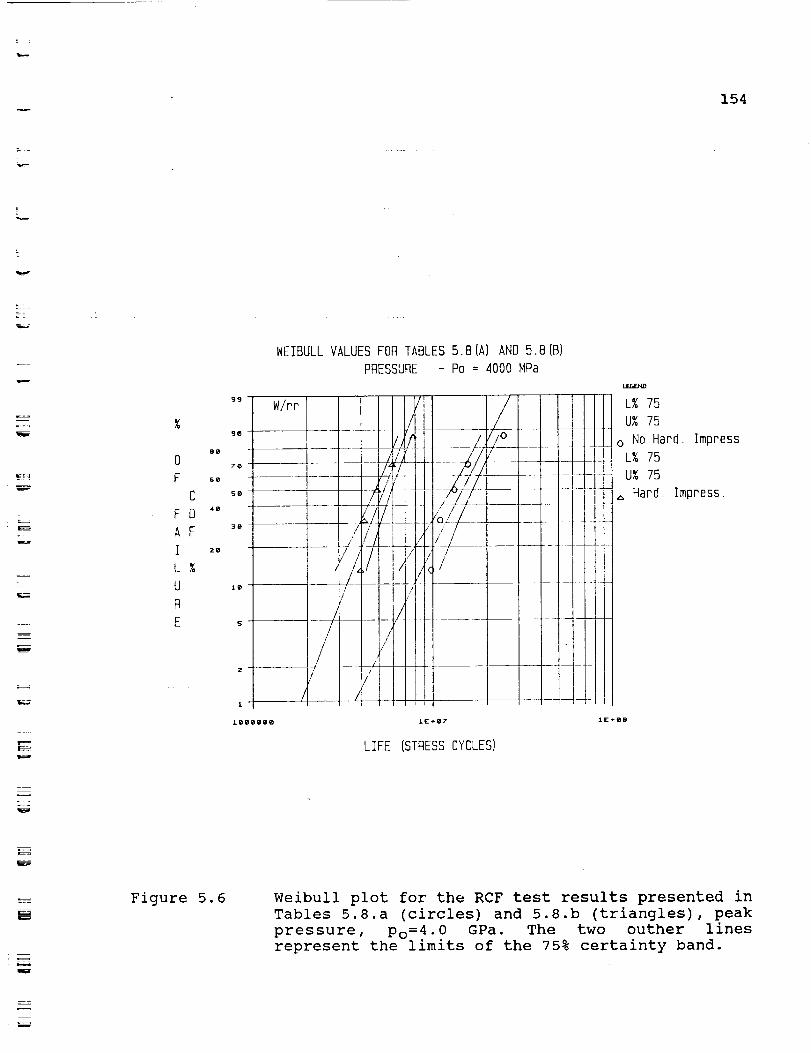
154

=

"_ L

B_

0

F _

C

F D ""

AF

I 2o

L

U

R

E

WEIBULL VALUESFOR TABLES5.B(A) AND 5.8(B)- Po = 4000 MPa

!

LIFE (STRESSCYCLES]

L% 75U% 75

o No Hard. ImpressL% 75

U% 75

Hard. Impress.

£E-06


Tables 5.8.a (circles) and 5.8.b (triangles), peak

pressure, Po=4.0 GPa. The two outher linesrepresent the limits of the 75% certainty band.

w

155

Table 5.9(a) Rolling experiment without hardness impression

(Do = 5450 MPa)Bm

Test Specimen Track Machine Hardness

# ID ID Head Indent

Ball Hours to Stress

Lot Failure Cycles

1 A7 L4 1 No R 8.1 4.17 x 106

2 A7 L5 1 No R 8.5 4.38 x 106

3 A7 L8 1 No R 7.2 3.71 x 106

4 A7 L9 1 No R 14.2 7.31 x 106

5 A7 LI0 1 No R 12.2 6.28 x 106

m

ml

Table 5.9(b) RollincLexperiment with hardness impression

(D e = 5450 MPa)

l

J



Spall Growth Life

in Stress Cycles

1 A7 LII 1 Yes R 0.695 x 106

2 A7 LI2 1 Yes R 1.210 x 106

3 A8 L1 1 Yes R 1.416 x 106

4 A8 L2 1 Yes R 2.678 x 106

5 A8 L3 1 Yes R 4.532 x 106

J

W

U

g

E,--U

W

156

Table 5.10(a) Weibull Darameters for rollina test without

hardness impression (Po = 5450 MPa)


1 0.3708 x 107 0.1294

2 0.4172 x 107 0.3147

3 0.4378 x 107 0.5000

4 0.6283 x 107 0.6853

5 0.7313 x 107 0.8706

Slope = 3.32260 LI0 = 0.29419 x 107

Intercept = -51.73905 L50 = 0.51865 x 107


Mean Life = 0.52146 x 107


Table 5.10(b) Weibull parameters for rolling test with

hardness impression _D o = 5450 MPa)


1 0.6953 x 106 0.1294

2 0.1210 x 107 0.3147

3 0.1416 x 107 0.5000

4 0.2678 x 107 0.6853

5 0.4532 x 107 0.8706

Slope = 1.38991


LI0 = 0.4812 x 106

L50 = 0.1866 x 107


Mean Life = 0.22133 x 107


w

157

mII

M

8_

0

F 6o

C

F D ""

A F

I 2e

L

U

R

E

89

It/

70

$8 --

[

1

_OOeO

WEIBULL VALUES FOR TABLES 5.11 AND 5.12


IlIlll

t II1_

HH 444L......I I I I'

tl]11

llll.....IlliI[X /lb1411--/:_.

it,:,,1

r J,_l!l !

!!i!l..../

/

m.


L% 75

U% 75

o N.H.I. + S.B.

L% 75

U% 75

H.I. + S.B.

W

=_

J

w

z

I

mIIF

w

W

W

Figure 5.7.a Weibull plot for the RCF test results presented in

Tables 5.10.a (circles) and 5.10.b (triangles),

peak pressure, Po=5.45 GPa. The two outher lines

represent the limits of the 75% certainty band.

i

L

%/.

{

V_

w

--4

158

with and without hardness impression 19, but employing smooth

ball_-_Tabl@s_5z_and_ _=!_ s_hpw the rolling test results and the

significant Weibull distribution parameters. The results are

presented in Weibull charts in Figure 5.7.b.

5.2.3 Spa!IReplication and Sectioninq Techniques: Before an

accurate 3-dimensional finite element model of a crack under

rolling contact loading can be implemented, more needs to be

known about the geometry of the spalls. Typical spall angles and

dimensions, as well as their relationship to the applied load,

the geometry of the system, the lubrication, etc., have to be

accurately defined. Spalls created during the experimental phase

of this program were studied using two different methods: a) a

replication technique, and b) a mechanical sectioning followed by

scanning microscopy observation.

The first procedure consists of the following steps: i) the

sample was degreased using methanol in an ultrasonic cleaner, 2)

a medium viscosity plastic material (vinyl polysiloxane) was then

prepared and applied on a glass microslide, 3) the sample, with

the spall under study facing down, was pressed against the

plastic and held in position for approximately 15 minutes, 4) the

sample was removed from the plastic. In order to check the

degree of fidelity with which this method reproduces the

topological features of the spall, the replicas were gold coated

and observed under the scanning electron microscope. Figure 5.8

shows photographs of a spall and the resulting gold coated

replica.

The samples were mounted on the adjustable stage of a Sloan

Dektak Surface Profile measuring device 20, which allowed up to

i00 #m displacement in the radial direction 21. The stylus of the

profilometer was positioned on the replica at a distance of

approximately 0.3 mm from the spall (this position was taken as

the origin in the y direction). The stage was moved along the

axial direction at a rate of 0.01 cm/min. Figure 5.9 shows traces

obtained with the profilometer, as well as their relative

location on the spall. A total of 18 traces were taken for each

spall at intervals of approximately 0.05 mm each. The traces were

then digitized and used to create a 3-dimensional drawing of the

19 Two samples were not used for the calculations because

they presented lives which were completely different from the

rest of the population.

20 This equipment has a sensitivity ranging from 25 Angstrom

units to a maximum of ixl06 Angstrom.

21 Relative to the spall, x is the axial direction, y is

the circumferential direction, and z is the radial direction.

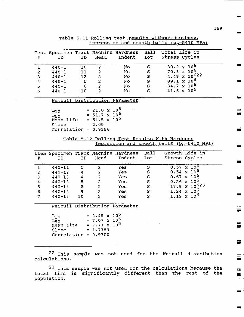
Table 5 II Rollinq test results without hardness

imDression and smooth balls (Do=5410 MPa)

159J

Test Specimen Track Machine Hardness Ball Total Life in

# ID ID Head Indent Lot Stress Cycles

1 440-1 i0 2 No S 30.2 x 106

2 440-1 ii 2 No S 70.3 x 106

3 440-1 12 2 No S 4.49 x 10622

4 440-1 5 2 No S 89.1 x 106

5 440-1 6 2 No S 34.7 x 106

6 440-1 i0 2 No S 41.6 x 106

i

I

W

Weibull Distribution Parameter

LI0 = 21.0 x 106

L50 = 51.7 x 106Mean Life = 54.5 x 106

Slope = 2.09


Table 5.12 Rollinq Test Results With Hardness

Impression and smooth balls (Po=54!0 MPaL

N

Item Specimen Track Machine Hardness Ball


Growth Life in

Stress CyclesU

440-LI 5 2 Yes S

440-L2 4 2 Yes S

440-L3 4 2 Yes S

440-L3 5 2 Yes S

440-L3 8 2 Yes S

440-L3 9 2 Yes S

440-L3 i0 2 Yes S

0.57 x 106

0.54 x 106

0.67 x 106

0.26 x 106

17.9 x 10623

1.24 x 106

1.19 x 106

=

W

Weibull Distribution Parameter

LI0 = 2.45 x 105

L50 = 7.07 x 105Mean Life = 7.71 x 105

Slope = 1.7789


22 This sample was not used for the Weibull distribution

calculations.

23 This sample was not used for the calculations because the

total life is significantly different than the rest of the

population.

m

im

==

U

m

I

zm

m

160

.... i_: :_:_

_==

m

B_

0

F 6e

C

F D _o

A F

I 2_

L

U

R

E

_e

70

5e

90

WEIBULL VALUES Fo-RTABLES 5.10 [A)- ANB5,10(B)


W/rrI 1 ' ' ' I I , v,........ . m --i

_ I I .........//_ __ __ .........

I

---- I ! I+---- -i

/

/,

/I I 4

-- I --

5 ..... _A_.I....

2

J.

LIFE (STRESSCYCLES)

L% 75U% 75

o No Hard. ImpressL% 75

U% 75

Hard. Impress.

:: : :7:= : ................. : :77 , =_ --

7

Figure 5.7.b Weibull plot for the RCF test results presented in

Tables 5.11 (circles) and 5.12 (triangles), peak

pressure, Po=5.41 GPa. The two outher linesrepresent the limits of the 75% certainty band.

ORIGINAL PAGE ISOF POOR QUALITY

161

(D

_h

E

U_

C

,-_ U_r-_ cJ

D_

.u

O

O C.,-4

UX

,-4 o

O_)._>

,-4 .

O_

C U

_ZLr--

co

i/3

U_.,H

ORIGINAL PAQE ISOF POOR QUALITY

gg

w

m

III

I

I

U

W

_ji

U

r

162

: ::

w

r

r

_LSCA_ 11_ 1_1cIlMK |M. 2('_!°_'$°/D1_-_1/OA,'I_N Iltl'Ag

{_ {¢,,'."W' / {I ,'J-'_ ,.

=

.==

Figure 5.9

ORIGINAL PAGE IS

OE POOR QUALITY

Traces of the spall's surface obtained with the

Dektak Surface Profilometer. The scales are indicated

in the figure, as well as the relative position of

the traces in the spall.

163

spall; Figure 5.10 shows thiscorresponding iso-contour map24.

drawing as well as the

Some effort has been devoted in the past to characterizingthe geometry of the spall failures. Shao et al. (1987) and Soda(1981) have reported cracks running at 20 ° to 30 ° to the surface.Bhat and Dolan (1982, 1983) have detected crack inclinations ofi0 ° to 20°; Voskamp (1988) has indicated the presence of cracksrunning parallel to the surface. Kumar et al. (1987), amongothers, have pointed out the following general features of thespalls: a) the V-shaped spalls point in the rolling (forward)direction, b) the cracks grow laterally and circumferentiallymaking a small angle with the running surface, c) the cracks growdeeper as they extend in the direction opposite to the rollingdirection, and present a stepped like character, d) the cracksbreak through to the surface at the shallow end, thus producing acantilever flap supported by an "unbroken" ligament at the deeperend, e) due to secondary cracks running perpendicular to the maincrack front, portions of the flap behind the crack front breakoff periodically producing wear fragments.

In order to systematically check these observations, spallsproduced for the present project were sectioned and observed ina transmission electron microscope. The sectioning was done witha high speed silicon carbide cutting blade; water was used as alubricant. Spalls were sectioned along the axial andcircumferential directions. After sectioning, the spalls weremounted in conducting resins (Conductomet) and polished withpolishing paper grits 240, 320, 400 and 600. Pictures were takenin a Hitachi scanning electron microscope.

Table 5.13 summarizes the results obtained from theobservations 25. Figure 5.11 shows a schematic representation of atypical spall and the nomenclature used for the differentdimensions and angles. Figures 5.12.a-d show spalls viewed alongthe radial direction and, after the sectioning, in thecircumferential direction. In the radial view, the presence of amicropit right before the V-apex of the spall is evident (Figure5.12.a). Figures 5.12.b and c show spalls formed in the vicinityof hardness impressions. The top views also indicate the presenceof a surface breaking radial crack; this can also be seen in thecircumferential cut. The linking of this radial crack with thehorizontal subsurface crack results in the detachment of another

24 The 3-dimensional drawing and the iso-contour maps arecreated by a Fortran program which makes use of the subroutineDISSPLA from Integrated Software Systems Corp.

25 All these results are for a peak Hertzian pressure of Po =

5.45 GPa, for which the semi-minor and -major contact widths are

w 2 = 0.22 mm and w I = 0.40 mm respectively.

l

m

n

mW

m

J

U

W

ml

m

im

m

mm

g

U

164

L--

0.3,'

Sample A7Spall L5

L

q_w

Figure 5.10 3-Dimensional digitized view of spall A7-L5

created under a pressure of Po=5.45 GPa. Thedigitized 3D view results from the traces

obtained with a surface profilometer on the

surface of the plastic replica. The projection on

a plane perpendicular to the radial direction

shows the height iso-contours in the spall.

Table 5.13 Spalls Geometry

165I

g

Samp. Track Hard. Ball Wmax

ID ID Imp. Lot (mm)

_max Lmax _o Cut @ D

Wth (mm) ( ) ( ) (mm)J

A1 L1 N R 0.965 1.20 0.72 62 C 21 0.096

A3 E1 Y R 0.824 1.02 0.78 54 C 21 0.130

A3 L2 Y R 0.929 1.15 0.86 62 C 20 0.149

A7 L1 N R 0.988 1.23 0.99 NA C NA 0.138

A7 L3 N R 0.812 1.00 0.34 NA C 20 0.075

A7 L7 N R 1.032 1.28 1.04 30 C 24 0.142

A7 LI0 N R 1.082 1.34 0.91 61 C 13 0.130

A1 L2 N S NA NA NA NA A 54/68 0.115

A1 L3 N R 0.747 0.93 0.57 55 A 21/45 0.089

A3 L3 Y R 0.845 1.05 0.85 50 A 44 0.142

A7 54 N R 0.853 1.06 0.95 30 A 67/65 0.089

A 53/60 0.130A7 L5 N R 0.952 1.18 1.12 45 A i0 0.075

A7 L8 N R 0.900 1.12 1.07 51 A 67/65 0.108

B

m

m

Wma x - Maximum width of the spall, along axial direction (mm).

Lma x - Maximum length of the spall, in the circumferential

direction (mm).

- Angle at the apex of the spall (°).

- Angle(s) observed in the respective cut (°).

D - Depth, maximum depth for the circumferential cuts, and

local depth for the axial cuts.

C - Circumferential cut.

A - Axial cut.

N.A. - Not available

All the tests included in this table were run at a peak Hertzian

pressure of 5.45 GPa.

mI

mm

m

m

i

i

w

mw

166

= .

7

w

\

WMAX

• )

R.D. \%_"

\ \ \ \ \ \ CIRCUMFERENTIAL CUT

(A-A)

i

.J

_V

i FBRADIAL VIEW

///__ "---_177;.,,I///////////,

AXIAL CUT

(B-B)

'ii

w

w

z:

w

Figure 5.11 Schematic representation of a spall indicating the

nomenclature used in Table 5.13, angles are

measured with respect to the -surface of the

sample.

-+

0 -_ ,_ _-,_r- ._

•_ . o0_

o

o % 0

.12

I C'd

<_ 0,12

,__ r- 0

_1 .,...1_ ,

(I) _-4• _-'t _ "'-'_

_.,_ ,-_

_ I _

-,-,I

167

ORIG_NAL PAGE |S

OF POOR QUALITY

im

n

I

ibm

Ill

g

=:=

m

I

i

I

I

J

W

168

z: ">_

• I1 •

x

o_00co _

_0 O_C_

× _0 0

_ _ .

_ _.

<

._ _ 0

""_ 0

> _._0

-_ 0 _ " _

_ _ 0

t_r_

ORIGINAL PAGE I$

OF POORQUALITY

169

/

0 _

o×__o0_ _z' _u]

,--4

o "_ Du_(D _n 0

_Z

I _ D-,

t_ 0

_) u_ o 43

> N ¢0

U

tD

us

43

u%

z:

0

C'ORIGINAL PAGE IS

OF POOR QUALITY

= _

L

u

!

w

_-_ _ u'_O-,_ '_

,_ •

×_o 0o0_

_3 _._

o _,_tn i_

,--i u 1_

o _ _J

O

t_.,H _-_• _ U D._ •

u_

0_

-,-'4

170

m

ORIG#NAL PAGE ISOF POOR' Q_JALIT_

171

cantilever flap. Figures 5.13.a-d show top views of several

spalls, as well as the result of axial sectioning. The axial cuts

reveal the presence of subsurface cracks propagating in theaxial direction.

5.3 Retained Austenite

The cyclic straining of the material under the contact may

induce the gradual transformation of the retained austenite

present in the matrix 26. Test Series 2, see Table 5.2, sought to

find a connection between the change in life and a probable

change in retained austenite content. However, any changes in

life are not obvious from the Table. More testing may be required

before any conclusions may be drawn.

5.4 Nucleation vs. Growth

Experimental measurements summarized in Figure 5.1427 show

that the life of ground, 440C steel rods employed by the 3-

ball-rod tester is reduced by about 10x when the conventional,

lapped balls are replaced by the standard rough balls recommended

for use with the testing machine. The installation of a 120 _m-

diameter, 30 _m-deep dent (Rockwell C hardness indent) reduces

the contact life with rough balls by an additional factor of 3xto 10x.

Since the effect of surface finish is confined to depths

comparable to the asperity height, the implications of these

results is that the lives of ground 440C bars obtained with the

rough balls (standard conditions) and with smooth balls are

controlled by the near surface mode. This is consistent with the

findings of Lorosch shown in Figure 5.15 for the 52100 grade.

This figure shows that only the elements with the longest lives,

i.e. N _ 108 contacts at Po = 5.4 GPa, are of the subsurfacemode.

The installation of artificial dents makes it possible to

follow the progress of spall nucleation and growth. Figures

5.16.a through c show the evolution of a surface initiated

defect, in the proximity of a hardness impression. These pictures

were taken from sample A6, subjected to Po=5.4 GPa, after 4, 6

and 10.3 hours (approximately 2.1, 3.1 and 5.3 million cycles

respectively). Figure 5.17 also shows the effect of a small

surface indent in the raceway of a sampie subjected to a rolling

contact pressure of Po/k=8.9.

26 The retained austenite may be as high as 45%.

27 This figure is obtained from the results presented in

Tables 5.5(a)-5.12.

mm

W

E

m

I

mm

l

i

m

I

l

w

I

t

R

u

m

i

F_

ORIGINAL PAGE IS

OF POOR QUALITY

r3 _ •

,_ ,_ _-._,-_

•_ D _ D._X _U_

_ N _ r'___-_

× _o

m

,---_ "_ %1=

_ _:L _

11) r-

N_U<D u_

_OCL

-,_ .__

_3

t'3

LR

-,-I

172

"O'U

=

x

q_

Xo

I X

<ul

%4o

.r..t

> _

"dr_ ul

_.,-i

-,-'t

173

,-4

,.Q

,.c:b",

0

...C

.,o.,-i3:

g

II0

0

ffl

,M

I1)

I

I

B

i

I

I

m

i

i

w

I

I


I

!

=I

i..a

L

w

--Z

w

T_

in

w

,,,--.

._ _-_X

rd _ ..Q

X _

t.n -,-t

_ -,.-t

I Np- _uq

m•,_ u_

_) tn• ,--i Ul

_-,_ _

0

1.4

-,-I

OR)G!N,_L PAGE IS

OF POOR QUALITY

174

175w

4-; r_

_-_'U

X

O

x X:_o4J4_i..,3 t.-- .,_.t

o N.w E

_g

I ×r._ IJ.) if5

t,')

p_. C_

0 030U

.u

"_" b']> ," _j

,--_ O m,

e"l

dtll

t_

I

m

m

I

u

n

mw

B

m

B

m

m

m

ORIGINALPAGEISOF POOROUAU'W j o

i

w

176

w

m

m

600O

5000-

9. 4000-

¢o

sooo-

dk

S - SMOOTH BALL_

R - ROUGH BALLS

orR

\%

2000 ........ , , ,' .... , , , , ..... , r' , , , .', ,,

ixl0 5 ixl0 6 Ixl0 7 IX10 8 ixl0 9

s_ress cycles

m

Figure 5.14 Fatigue lives versus contact stress level for

440-C RCF test samples. Note: these are the

nucleation and growth lives for unindented

samples. _ The lives for dented samples are

approximately equal to the growth part because

nucleation is very short. The keys for the figure

are indicated in the graph.

177mm

mm

g

wm

mm

--D

8

_C

3.

_) N_te: The subsurface shakedown

pressure 2424

\\_-_ " " " k - 606 ._: P'o"_k= MPa

__ oO_ _ A,B'- Subsurface failures

-_ \\ .... - _. _.o._o._o_.o_o_o_ ""...4

•_ -,_-.... ..... _,

= '-2400 _ Subsurface Shakedown

' _'"ib" _ ' "_.... Io' _ ' _ .... '_9 _ _"_'° _ " ' S ,(_"

LIO- Contact Life, Numbers of Contacts

u

I

_-m

_j

/

J

mi

m

!

J

Figure 5.15 Cyclic lives and shakedown pressures for near-

surface (C,D) and subsurface rolling contact

failures (A,B) in steel 52100 after Lorosch

(1987). Results labeled (C) are for I00 _m surfaceindents.

i

l

m

mm

178

%,-.

w

"Ill"

=

r,-

I

J ; •

.;_ - ,R.D.

_CC_

0_0_

r_

_" _0

.-.._4J •

_:_.,._ __ •0 _)4 J oJ

_5_ C

_-,'_ U')""..t.2,

(D k4 _ ._

>_ .C _ 4J m

_4Jr_01_

_3

,-4


179

_o

D

, =

i

=

u

I

w

ORIGINAL PAGE IS

OF POOR QUALITY M

I==

!

w

w

180

.EXb_JO0

•_ D_

E'-'O

0

_0 _

% _"_I1) (ll.C4J "_4J u,q"-"(])

_ U].C@4J

"_ b'_ ul -,_

b3 4J C

N4_O

0 _ ,--_ .,-_

0-_ _

C)

Lo

C_

ORIGINAL PAGE ISOF. POOR QUALITY

181

The growth life, N G, is defined as the portion of the total

life consumed by the cyclic growth of a I0 _m-surface crack into

a full fledged spall, as seen in Figure 5.17. The corresponding

initiation life, N I, is obtained by subtracting N G from the total

life, N, obtained by testing samples without a dent. The studies

have shown that the growth life is relatively insensitive to the

surface conditions and becomes a smaller fraction of the total as

the severity of surface defects is reduced. In the case of the

ground 440C steel rods tested at Po = 5.4 GPa, NG/N = 0.4 for

rough balls and NG/N = 0.02 for smooth balls. The conclusion is

that the cyclic growth of £he spall can dominate the contact lifeof the near-surface initiated cracks when the surface is rough

or damaged; nucleation of the spall dominates when the surface is

smooth and undamaged.

Preliminary studies show that nucleated cracks fail to grow

at a contact pressure of Po = 2.4 GPa. This result points to the

existence of a threshold for growth.

5.5 Surface Roughness

DeMul (1987) and Hamrock (1990), among others, have pointed

out the important role played by surface asperities, bumps,

grooves and dents in the near-surface failure mode. These defects

cause stationary pressure spikes, conditioned by "micro" EHDL

effects and produce peak amounts of plasticity at depths

corresponding roughly with the surface regularity depth or height

(2 to 20 #m) below the surface.

Surface roughness features of the specimens and balls are

characterized by peaks and valleys caused during the surface

preparation. Figure 5.18 shows the running surface on specimen

A6-L2: a) after 0.26 million stress cycles, and b) after 2.73

million cycles, c) spall formation after 10.09 million stress

cycles. Examination of the running surface on the specimens

indicates that small surface roughness features are gradually

smoothed out with ' ......' ........................................................increaslng numbers of stress cycles. However,

deeper and more prominent features persist even after 15 million

cycles. Similar observations are valid for the case of the

roughened balls used in the RCF tests. The prominent peaks and

valleys persist for millions of cycles and represent possible

crack initiation sites. There is evidence (Fighre 5.19) that

nearby located microspalls may link together, thus providing the

initial site for crack initiation.

W

L..

m

mm

l

W

i.

m

l

5.6 Replication and Metallographic Studies of Spalls in 440C

There is a need for a more detailed description of the 3-

dimensional geometry of the spalls, as well as of the different

crack propagation mechanisms leading to that geometry. There have

been previous three dimensional analyses of cracks under rolling

I

D

u

,,,,--

a

c d

182

_=

Figure 5.17 Effects of a small, 120 _m dent (A) in the raceway

of a bearing steel RCF sample subjected to rolling

_=_contact at Po/k=8.9. (a) dent [A] before test, (b)crack nucleus [B] is visible on surface after N =0.62xi06 contacts, (c) N = 1.3x106 contacts, and

(d) spall [C] forms after N = 1.5x106 contacts.

The rolling direction is also indicated, i.e.R.D.

ORIGINAL PAGE IS

OF. POOR QUALITY

a b

183w

i

I

I

ORIGINAL PAGE IS

OF POOR QUAUTY

Figure 5.18

"i

Backscattered electron image of the specimen

running surface (A6TL2), after (a) 0.26xi06

cycles, (b) 2.73xi06 cycles, and (c) lower

magnification secondary electron micrograph of the

spall formed after 2.73xi016 cycles. The boxed

area shown in (c) is the location chosen for the

micrograph in (a) and (b). The rolling direction

is also indicated, i.e.R.D.

184

r .

w

Figure 5.19 Micrograph of the running surface of the 52100 RCF

test balls showing two nearby located microspalls

linked together.

ORIGINAL PAGE IS

OF POOR QUALITY

185

contact by Kaneta and Murakami (1985a, 1985b, 1985c, 1986, 1987).

Although these address the problem of the lubricant induced

opening mode and crack face friction, they failed to consider the

cyclic plasticity induced under rolling contact loading.

The top view and circumferential cuts shown in Figures

5.12.a-d, reveal several important features: a) the cracks seem

to have initiated at micro-pits near the tip of the spall (this

is provided in the cases of Figures 5.12.b and c by the hardness

indentation), b) the crack at the V-apex slightly undercuts the

surface, thus indicating a small amount of crack propagation in

the reverse direction (more evident in 5.12.a), c) the main

cracks propagate at a shallow angle from the surface up to a

depth of approximately 60-80 #m (evidence suggests that the crack

front is straight along the axial direction and diverges from the

initiation point at an angle of 50 ° - 60°), d) the cracks then

propagate parallel to the surface for 130-200 _m, after which

they change direction to an angle of 45 ° from the surface, e)

this process is apparently being repeated cyclicly as evidenced

by the unbroken flap still attached at the tip of the spall

(clearly seen in 5.12.a).

The micrographs shown in Figures 5.13.a-d present axial cuts

of different spalls. These figures suggest that subsurface crack

propagation may also take place along the axial direction, as

evidenced by the unbroken flap still attached to the surface. The

results in Table 5.13 indicate that the maximum spall width is

larger than the Hertzian (elastic) contact width, however the

spalls were always confined to the wear track. Although some

degree of conformity ("sink in") is expected to occur between the

rod and ball, due to plastic deformation of the rod, the

experimental evidence suggests that the balls are oscillating

along the axial direction. This out-of-plane oscillation, and its

associated shear tractions, may provide the necessary driving

force for the subsurface, axial crack propagation.

This cyci_c change _n d_frections would indicate that once the

crack has been surface initiated by the micro pressure spikes,

its propagation is the result of more than one mechanism. Bower

(1988) has indicated that the fluid entrapment mechanism would

play an important role in crack propagation. However this

mechanism predicts that the crack would turn down, away from the

surface, which is not supported by our experiments.

The complicated non-proportional cycle of modes I and II

stress intensities at the tip of the crack is more likely to be

dictated by a combination of the entrapment mechanism and the

resolved cyclic in-plane shear stress. Additionally, the cyclic

bending to which the unbroken flap is subjected may favor the

formation of cracks connecting the main crack to the surface.

5.7 Rolling Contact of Hardened Aluminum

D

i

m

u

&&

=

l

m

mI

U

m

D

mm

m

u

U

w

186

w

w

m

ira--

t

m

w

w

Rolling tests and finite element calculations using

properties of 7075-T6 aluminum have been carried out as part of

the present project. Aluminum was chosen primarily because the

damage to the microstructure resulting in sub-surface crack

formation is easily obtained within a short testing time, t = 0.5

- 2.0 hours. In the case of 440C steel, much longer hours of

operation are needed to cause crack initiation. Moreover, post-

failure electron microscope studies of the spalls would indicate

that they are primarily surface initiated cracks.

Additionally, the cyclic stress-strain hysteresis response of

7075-T6 aluminum is qualitatively similar to 440C bearing

steels, as indicated in previous sections. Therefore, aluminum

proves to be an ideal material to study sub-surface originated

failure under rolling contact.

The experiments and calculations performed on this material

lead to the following conclusions:

i) The depths at which cracks are observed to form in the RCF

test samples are observed to correlate well with the maximum

depth at which the maximum cyclic plasticity is calculated, see

Figure 3.4.11. Subsurface crack initiation may play a more

important role in this material. The accumulation of damage in

the plastically strained region extending to a depth of 0.5w

below the surface as shown in Figure 3.4.10, conc'irrent with a

smoothing out of surface defects 28, leads to the translating

Hertzian pressure dominated failure.

2) The region where the largest number of cracks is observed is

the region where the residual stresses are not compressive and

there is still some cyclic plasticity, see Figure 3.4.12.

Compressive stresses inhibit cyclic crack growth by enhancing the

frictional dissipation between the faces of the crack.

5.8 Conclusions

No connection was found between the amount of retained

austenite and the life of the rolling element. More testing may

be required before any conclusions may be drawn.

The cyclic growth of the spall dominates the total life of

the elements with surface initiated cracks, when the surface is

rough or damaged. Nucleation is the controlling event in those

samples with smooth and undamaged surfaces.

Surface asperities, grooves, dents and bumps introduced

28 This material shows strong evidence of lateral flow, i.e.

plohghing, due to the rolling loading.

187

during manufacturing of the sample, play an important role in thenear-surface failure mode. Prominent features are not smeared outeven after several million cycles, thus providing sites for thehighly localized, cyclic pressure spikes responsible for failure.

....The 3-dimensi-o-n-al .....features displayed by the spalls wouldindicate that the surface initiated cracks would propagatedriven by several mechanisms. The individual contribution of thecomplicated, non-proportional cycle of Modes I, II and III,remains to be determined, and it certainly warrants furtherresearch in this area.

w

m

J

mm

u

i

mm

m

==.

m

mm

mm

m

J

J

J ,

w

w

r

m

• GENERAL DISCUSSION

188

_ 6.1 Finite Element Calculations of Con£act Plasticity

The contact plasticity has 2 components: (i) the transient

part which is responsible for the radial displacements and

residual stresses and (ii) the steady state or continuing

plasticity which leads to damage accumulation and crack

nucleation• There is evidence that the ELKP-model, which

confines the transient to the first contact cycle, does not

describe the transient adequately. The residual stresses for 2-

dimensional, line contact derived from finite element calcula-

tions with ELKP-properties understate the peak residual stresses

by a factor of _ 3 and place the peak at a relative depth of z/w

= 1.3 instead of at z/w = 0.8, where it is observed (Hahn et

al., 1987)• Recently, the authors have treated the 2-dimensional

contact with the more sophisticated, non-linear, Mroz-type, 2-

surface representation devised by McDowell (McDowell, 1985,

Howell, 199i). In this case the transient extends over 15 and

possibly more contacts, and while the residual stresses peak at

the correct depth, the extrapolated values of the residual

stresses are _3 times larger than the actual values• The steady

state cyclic plasticity obtained with the non-linear model agreeswith the results obtained with ELKP-behavior. It should also be

noted that the 3-dimensionalcontact plastic zone observed in the

aluminum samples in Section 3.4 is in good accord with the ELKP-

calculations. These findings support the view that the

descriptions of the continuing cyclic plasticity derived from the

finite eiement calculations with ELKP-properties are reliable.

However, the cyclic constitutive relations require more work to

provide reliable descriptions of the transient and the residualstresses.

While a single set of ELKP-properties has been used so far

to characterized hardened steel, it must be noted that the

kinematic yield strength, aK, is sensitive to microstructure. An

ongoing study by the authors shows that a K decreases by about 45%

at room temperature as the amount of retained austenite increases

from 16% to 4§%. The los s of cyclic strength is accompanied by a

more than 10-fold increase in the cyclic life and both of these

changes occur even though the retained austenite is transformed

by the cyclic deformation. While increases in the rolling

contact life with retained austenite have been reported for 52100

steel, these could not be demonstrated in the present work on440C steel•

As demonstrated by the 3 dimensional finite element

calculations, the addition of a sliding component with heating,

results in the introduction of tensile surface residual stresses.

The peak value of cyclic plasticity takes place at approximately

the same depth as for 3-dimensional pure rolling, i.e. z/w I =

w

189

0.329 , with approximately the same magnitude. However, the

sliding component causes a non-zero cyclic plastic component at

the surface. The combined effect of the tensile residual stresses

and the cyclic plasticity may lead to an exhaustion of ductility,

i.e. damage accumulation, thus giving support to the concept of

surface originated spall failure (see Section 6.2).

6.2 Spall Nucleation

The present study demonstrates that the spall nucleation

component dominates the rolling contact life when the contact

surfaces are smooth, defect free and well lubricated. The work

also shows, in agreement with previous studies, that modest

changes in the surface roughness of the counterface alter the

contact life by =10-fold. The relatively large indents affect a

=60-fold reduction in the contact life. These findings are

consistent with recent analyses of the effects of surface

irregulaties, which show that submicron-size grooves or

asperities can produce large stationary pressure spikes near the

defect (Goglia et al., 1984; de Mulet al., 1987; Hamrock, 1990).

Rolling-plus-sliding, with attending frictional tractions, also

produces more plasticity closer to or at the surface. As

illustrated in Section 3.5, even larger amounts of near-surface

plasticity that compete with the peak subsurface values are

generated when the sliding is accompanied by intense frictional

heating. Either individually or in combination, surface irregu-

larities, sliding and frictional heating can shift the region of

peak plasticity and damage from the subsurface to the near-

surface, thereby altering the mode of spall failure. Work must

be done to treat the plasticity arising from surface

irregularites so that this major contribution can be factoredinto the analysis of nucleation.

The large reduction in the contact life produced by small

indents may provide a means for accelerating contact testing.

Service life is frequently limited by indents from debris or

tramp abrasive particles and natural asperities. Consequently,rolling contact tests might prove more meaningful, and be of

shorter duration, if the test samples were fitted at the start

with well designed and pedigreed surface defects. This concept

is exploited in the 3-ball-rod test which is designed to be

conducted with artificially roughened balls. To provide a

further test of this idea, the correlation of the nucleation

lives obtained with and without defects should be examined. The

contribution of inclusion particles may be a complicating factor

here. This is because the cyclically deformed volume produced

by a small, isolated, surface irregularity is so small that the

Q

w

w

i

m

m

29 Where w I is the semi-major half-contact width; this is

equivalent to z/w2= 0.53, in terms of the semi-minor half-contactwidth.

rl

w

m

=

w

L

= =_

w

190

likelihood of an interaction with an inclusion particle is

greatly reduced.

In order to perform quantitative treatments of the spall

nucleation life, the accumulated damage produced by the

continuing cyclic plasticity and the conditions for crack

nucleation must be treated. The studies performed on aluminum

samples illustrate the complicated nature of the subsurface

nucleation process. The results indicate that neither the rates

of nucleation nor the rate Of crack growth correlate with the

amounts of cyclic plasticity. The findings suggest that residual

stresses may be playing an important role. The reasons for the=104-fold shorter crack nucleation lives at the same relative

contact pressure displayed by the hardened aluminum compared with

steel are not clear. It is possible that the higher homologous

temperature of the aluminum tests and resulting greater atom

mobility may facilitate microstructural changes leading to crack

nucleation. Since microstructural changes also play a role in

the nucleation of failure in steel (Swahn et al., 1976), the

stability of specific microstructural elements may affect

nucleation.

6.3 Growth and Spalling

The present study shows that the spall growth life is in the

range N = 106 to 107 contacts, and is relatively insensitive to

the condition of the surface. Similar results have been reported

by Shao et al. (1987) for carburized steel. The implication is

that the spall growth component is a large fraction of the total

life when nucleation is "easy" and the total life is short, e.g.

N < 107 contacts, and a tiny fraction of the total life when nu-

cleation is difficult and the total life is long, e.g., N = I0 I0

contacts. The tests also offer evidence of a threshold for crack

growth, i.e., crack nuclei about i0 _m-long on the surface failed

to grow at a contact pressure P0 = 2.4 GPa.

The fracture mechanics analyses examined in Section 4 reveal

that the Hertzian stresses, centrifugal stresses, thermal stres-

ses and the pressure of fluid in the crack cavity all contribute

to a complex supperposition of Mode I, Mode II and Mode III

crack driving forces. However, the largest contribution appears

to be the Mode I driving force resulting from the fluid pressure.

Further, it appears that 2-dimensional models of the 3-

dimensional crack overstate the driving force.

To critically test these findings, fracture mechanics calcu-

lations of the spall growth life were carried out for the condi-

tions in the 3-ball-rod testing machine, and compared with the

L=

w

191

measurements of the 440C growth life 30 . The results are

presented in Figure 6.2. They show that the fracture

calculations predict both the spall growth lives, at least within

an order of magnitude. They also predict the existence of a

threshold at roughly the observed contact pressure. Considerable

uncertainty is involved in the calculations since the da/dNcharacteristics of the 440C steel were not known and the details

of the dimensional growth were not considered. Further, the Mode

II driving force was neglected. Consistent with this, the

calculated lives are longer than the measured ones.

The metallographic observations of a step-wise growth

suggest that the spall advances into the surface with the lateral

sides of the spall attached. At a later stage the latteral sides

rupture converting the spall into a loose flap. After

propagating parallel to the surface for a short distance, the

spall branches away from the surface. Simultaneously, a crack

seems to initiate from the surface attending to the cyclic

tensile stresses due to the bending of the loose flap (Figure

5.12a). This sets the stage for the formation of the first spall

fragment. With the lateral portions of the remaining branch

still intact, this branch resumes growth into the material until

the lateral connections again break to produce a flap. One

important difference is that large, rising and falling pressure

spikes are expected to form around the cavity left by the first

spall fragment. These pressure spikes will contribute to the

crack driving force and accelerate the pace of spall growth.

6.4 Conclusions

(i) The findings reported here, taken together with other

recent work, support the view that the descriptions of

continuing cyclic plasticity derived from finite element

calculations with ELKP-properties are reliable. However, the

treatment of the cyclic constitutive relations must be improved

to obtain reliable descriptions of the transient and the residual

stresses.

m

mW

J

i

I

W

U

u

g

m

30 The total number of stress cycles was calculated by

introducing the Mode I crack driving force derived in Section 4.4

(Equation 4.1) into a Paris' type equation, i.e. da/dN = A(_K) n.

The constants A and n fit the stage II portion of the results

obtained by Bamberger et al. (1982), for different bearing steels

(refer to Figure 6.1 and Table 6.1). Numerical integration was

carried out assuming an initial crack nucleus of, a o = i0 _m, and

a final crack length of, af = 240 _m. Small departures from the

linear, stage II, portion of the resistance curve lead to a large

(3 - 4 orders of magnitude) increase in total number of stress

cycles. This can be related to the pressence of an effective

threshold to crack propagation.

m

mI

i

I

i

U

K-

in

192

L _

w

w

(ii) Either individually or in combination, surface

irregularities, rolling-plus sliding and frictional heating can

shift the region of peak plasticity and damage from the

subsurface to the near-surface, thereby promoting near-surface

spall failure.

(iii) The spall nucleation component dominates the rolling

contact life of 440C steel when the contact surfaces are smooth,

defect free and well lubricated. Small surface irregularities

reduce the nucleation life drastically.

(iv) The possibility of accelerating rolling contact testing

by fitting samples at the start with well designed and pedigreed

surface defects deserves further study.

(v) Studies using hardened aluminum as a model material

suggest that residual stresses, atom mobility and the stability

of microstructural elements affect the nucleation life.

(vi) The spall growth component is a large fraction of the

contact life when nucleation is "easy" and the total life is

short, e.g. N < 107 contacts, and it is a tiny fraction of the

total life when nucleation is difficult and the total life is

long, e.g. N = i0 I0 contacts.

(vii) The experiments provide evidence of a threshold for

crack growth.

(viii) The measurements of the spall growth life are in

reasonable accord with fracture mechanics predictions based on

the Mode I component of the crack driving force generated by 3-

dimensional cracks with fluid pressure in the crack cavity. The

calculations predict both the growth lives within an order of

magnitude and the existence of a threshold close to the observed

contact pressure.

w

193 ..

w

I

i

2 3 4t0 .3 _-I I I

O_4U

m

_ 10-5

_ 10 -6

u

_ I0 zu

io .8

5 6I I

AK, Ksi.in I/2

7 8 9 I0 t5 20 25I I I I I I I •

X

/X

/

Foticjue Crock Growlh RotesM-50 ond M-50 NiL

Auslenil ized 1095 =C

o M-.50 Tempered 540°C x 3x M-50 Tempered 540°C x 5

• M-50 Tempered650°Cx 5

• M-5ONiL Tempered 540°Cx5

__1 .... 1 ___1 ___1.... _1___l__J_[ 1 I I l3 4 5 6 7 8 9 I0 i5 20 25 30 40

Alternating Stress Intensity, AK, MPa " m 1/2

10-,5

10 .6

&lp.((J

(J

10-7 ._=-

10"8

10-9

I

I

I

I

II

I

I

i

I

mI

Figure 6.1 Resistance curves for different bearing steels,

after Bamberger et al. (1982). Additional

information is presente in Table 6.1.

I

w

I

Table 6.1 Heat Treaments and Fracture Toughness

Data for Bearing Steels, after

Bamberger et al. (1982).

194

Steel Heat Hardness AKth KicTreatment Rc (MPa.Jm) (MPa.Jm)

M50 A 63 3.1 17.7

M50 B 61 4.2 23.0

M50 C 43 5.0 48.0

M50 D 44 3.8 51.0

v

w

m

w

Heat Treatment

A Austenitized at 1095 °C

Tempered at 540 °C, 3 times.

B

C

Austenitized at 1095 °C


Austenitized at 1095 °C


D Austenitized at 1095 °C

Cooled at -85 °C


z

w

195 i

I

6000

o_ 500C

vl

CL 4000

0(I)

3000

2000

10'

Fatigue Life vs Contact Stress

SMOOTHBALLS

Legend

GROWTH LIFE

• GROWTH LIFE

P'_ CALCULATED

........ i

ROUGHBALLS

10' I0'°

Sfress Cycles

I

I

I

W

I

I

w

I

I

iI

Figure 6.2 Fatigue Life (number of stress cycles to failure)

versus the Contact Stress (peak Hertzian pressure)

for bearing steel 440C. The figure indicates the

experimentally obtained growth lives obtained for

tests run with rough and smooth balls. The band

represents the upper and lower limits for the

total number of cycles caiculated using the

results from Section 4.4, and the data from Figure

6.1 and Table 6.1.

w

I

i

I

i!

I

w

-- =w

L_

L__T

=

196

7. CONCLUSIONS

The following general conclusions can be drawn from the work

performed for the present contract:

The ELKP-parameters derived from the hysteresis loops of the

440C steel are similar to those previously reported for hardened

AISI 1070 and 52100 bearing steels. After correction for strain

rate effects, a k = 1050 MPa and M = 188 GPa.

The resistance of aluminum 7075-T6 under cyclic torsion is

1/3 to 1/2 of that displayed by 440C steel. However the

hysteresis loops reveal a kinematic behavior analogous to the

440C.

Hardened aluminum proves to be a reasonably good model

material. Cyclic plasticity can be revealed metallographically,

subsurface failure takes place after a moderate number of stress

cycles, even at low contact pressures. These qualities may

provide opportunities for: i) studying the effects of residual

stresses, ii) verification of constitutive formulations, iii)

testing fracture mechanics approaches to spall growth analyses.




pressures of Po/kk _ 4.0, 6.6 and 8.9, using the geometry of the

three ball/rod contact fatigue testing machine. The subsurface

stresses, plastic strains, residual stresses and plastic work

done are evaluated. Equivalent stresses above the kinematic yield

strength extend to the surface only for the highest load level.

The peak equivalent plastic strain occurs at approximately 0.25w 1

(Wl/W 2 = 1.77) for all load cases; the values of these strainsare 4.4xi0 -4, 2.33xi0 -3, and 4.0x10 -3, for the low, medium and

high loads, respectively.



properties of the 7075-T6 aluminum alloy, at a relative Hertzian

pressure of Po/kk = 5.7, using the geometry of the three ball/rod

contact fatigue testing machine. The subsurface stresses, plastic

strains, and residual stresses are evaluated. The peak plastic

strain amplitude, _£Pmax/2 = 1.6x10 -3, occurs at a relative depth

of z/w = 0.4 below the surface. Peak residual stresses obtained

are arx(max) = 26.4 MPa, and ary(max) = 39.7 MPa, occuring at arelative depth of z/w = 0.9.

Two dimensional finite element calculations of repeated

rolling-plus-sliding contact have been carried out for ELKP

properties of an AISI 440C beiring steel, at relative Hertzian

pressures of Po/kk = 5.0. Plastic strains, residual stresses andtemperature distributions are presented. Plastic strains are

w

197

shown to be considerable lower for ELKP properties than they for

an elastic-perfectly-plastic material (Kulkarni et al., 1989).

Steep temperature gradients close to the surface produce high

compressive stresses; the ensuing cooling causes residual tensile

stresses, a possible mechanism for thermo-cracking. Thermo-

mechanical behavior is highly dependent on the material

properties, which also may be temperature dependent. A more

precise definition of these properties, especially the thermal

film coefficient, is recommended.

Efforts have been made to extend the Bower treatment of 2-

dimensional, surface breaking cracks with fluid in the crack

cavity to smaller relative crack lengths but the Bower algorithm

proved unstable for a/w < 0.5. In the range 0.5 < a/w < 1.5, the

values of the normalized driving force, K/PoJa , decrease with

the relative crack length, a/w, for lubricated contact, but

increase for dry contact.

A compilation of _K-driving force values of surface

breaking cracks has been assembled. This reveals that fluid in

the crack cavity, centrifugal stresses, and thermal stresses add

significantly to the crack driving force, particularly for

relatively short cracks, a/w < 0.I. Fluid in the crack cavity is

especially potent, producing relatively large Mode I driving

force values. The driving forces generated by 3-dimensional

cracks are -20% of the values calculated for 2-dimensional

cracks.

As a result of the modest driving force generated by small,

3-dimensional cracks, surface cracks as large as a -i0 _m would

not be expected to grow in idealized smooth, well lubricated

bearings with a Mode I, _KTHR_SH = 5 MPa subjected to a Hertzian

Pressure, P0 = 2.4 GPa. Thls is consistent with experimentalresults described in Section 5.4.

No connection was found between the amount of retained

austenite and the life of the rolling element. More testing may

be required before any conclusions may be drawn.

The cyclic growth of the spall dominates the total life of

the elements with surface initiated cracks, when the surface is

rough or damaged. Nucleation is the controlling event in those

samples with smooth and undamaged surfaces.

Surface asperities, grooves, dents and bumps introduced

during manufacturing of the sample play an important role in the

near-surface failure mode. Prominent features are not smeared out

even after several million cycles, thus providing sites for the

highly localized, cyclic pressure spikes responsible for failure.

The 3-dimensional features displayed by the spalls would

indicate that the surface initiated cracks would propagate

I

I

I

!

I

I

i

I

I

mI

im

!

I

I

i

3

r--

198

driven by several mechanisms. The individual contribution of the

complicated, non-proportional cycle of Modes I, II and III,

remains to be determined, and it certainly warrants furtherresearch in this area.

The findings reported here taken together with other recent

work support the view that the descriptions of continuing cyclic

plasticity derived from finite element calculations with ELKP-

properties are reliable. However, the treatment of the cyclic

constitutive relations must be improved to obtain reliable

descriptions of the transient and residual stresses.

Either individually or in combination, surface

irregularities, rolling-plus sliding and frictional heating can

shift the region of peak plasticity and damage from the

subsurface to the near-surface, thereby promoting near-surface

spall failure.

The spall nucleation component dominates the rolling contact

life of 440C steel when the contact surfaces are smooth, defect

free and well lubricated. Small surface irregularities reduce the

nucleation life drastically.

The possibility of accelerating rolling contact testing by

fitting samples at the start with well designed and pedigreed

surface defects deserves further study.

Studies using hardened aluminum as a model material suggest

that residual stresses, atom mobility and the stability ofmicrostructural elements affect the nucleation life.

The spall growth component is a large fraction of the

contact life when nucleation is "easy" and the total life is

short, e.g. N < 107 contacts, and it is a tiny fraction of the

total life when nucleation is difficult and the total life is

long, e.g. N _ i0 I0 contacts.

The experiments provide evidence of a threshold for crack

growth.

The measurements of the spall growth life are in reasonable

accord with fracture mechanics predictions based on the Mode I

component of the crack driving force generated by 3-dimensional

cracks with fluid pressure in the crack cavity. The calculations

predict both the growth lives within an order of magnitude andthe existence of a threshold close to the observed contact

pressure.

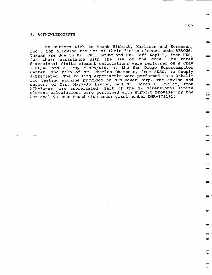
n

8. ACKNOWLEDGMENTS

199

The authors wish to thank Hibbitt, Karlsson and Sorensen,

Inc., for allowing the use of their finite element code ABAQUS.

Thanks are due to Mr. Paul Leung and Mr. Jeff Koplik, from HKS,

for their assistance with the use of the code. The three

dimensional finite element calculations were performed on a Cray

X-MP/48 and a Cray Y-MP8/648, at the San Diego Supercomputer

Center. The help of Mr. Charles Charmman, from SDSC, is deeply

appreciated. The rolling experiments were performed in a 3-ball-

rod testing machine provided by NTN-Bower Corp. The advice and

support of Mrs. Mary-Jo Liston, and Mr. James D. Fidler, from

NTN-Bower, are appreciated. Part of the 2- dimensional finite

element calculations were performed with support provided by the

National Science Foundation under grant number DMR-8721915.

mu

u

n

mw

m

I

J

u

mm

w

baF

w

m

2OO

References

ABAQUS, 1989, "User's Manual - Version 4.8", Hibbitt, Karlsson

and Sorensen, Inc, Providence, R.I.

Archard, J.F., 1959, "The Temperature of Rubbing Surfaces", Wear,

Vol. 2, pp. 438-455.

Bamberger, E.N., Averbach, B.L., and Pearson,

Improved Fracture Toughness Bearings",

AFWAL-TR-83-2022, AFWAL/POSL, WPAFB, Ohio.

P.K., 1982, "

Interim RePOrt,

Barber, J.R., 1967, "The Influence of Thermal Expansion on the

Friction and Wear Process", Wear, Vol. i0, pp. 155-159.

Barber, J.R., 1968, "Thermal Effects in Friction and Wear",

Dissertation, Cambridge University.

Barber, J.R., 1969, "Thermoelastic Instabilities in the Sliding

of Conforming Solids", Proc. Roy. Soc., Series A, Vol. 312,

pp. 381-394.

Barber, J.R., 1971a, "The Solution of Heated Punch Problems by

Point Source Methods", Int. J. Eng. Sci. Vol. 9. pp. 1165-1170.

Barber, J.R., 1971b, "The Effects of Thermal Distortion on

Constriction Resistance", Int. J. Heat Mass Transfer, Vol.

14, pp. 377-393.

Barber, J.R., 1972, "Distortion of the Semi-infinite Solid due to

Transient Surface Heating", Int. Jou. Mech. Sci., Vol. 14,

pp. 377-393.

Barber, J.R., 1973a, "Indentation of the Semi-infinite Elastic

Solid by a Hot Sphere", Int. J. Mech. Sci., Vol. 15., pp.

813-819.

Barber, J.R., 1973b, "Letter to the Editor", Wear, Vol. 26, pp.

425-427.

Barber, J.R. , 1976, "Some Thermoelastic Contact Problems

Involving Frictional Heating", The Quarterly Journal of

Mechanics and Applied Mathematics, Vol. 29, pp. 9.

Barber, J.R., 1980a, "Some Impiications of Dundurs' Theorem for

Thermoelastic Contact and Crack Problems", Journal of

Mechanical Engineering Science, Vol 22., No. 5, pp. 229.

Barber, J.R., 1980b, "The Transient Thermoelastic Contact of a

Sphere Sliding on a Plane", Wear, Vol. 59, pp. 21-29.

u

201 ..

Barber, J.R., and Martin-Moran, C.J., 1982, "Green's Functionsfor Transient Thermoelastic Contact Problems for the Half-

plane", Thermomechanical Effects in Wear, pp. 11-19.

Bastias, P.C., Hahn, G.T., and Rubin, C.A., 1989, "Finite Element

Modelling of Subsurface, Mode II Cracks Under Contact

Loads", Eng. Fracture Mechanics, Vol. 33. pp. 143-152.

Bastias, P.C., 1990, "Analysis of Cyclic Crack Growth Under

Rolling Contact Loading Conditions", Ph.D. Dissertation,

Vanderbilt University.

Bhargava, V., Hahn, G.T., and Rubin, C.A., 1985a, "An Elastic-

Plastic Finite Element Model of Rolling Contact. Part i:

Analysis of Single Contacts", ASME Journal of Applied

Mechanics, Vol. 52, No. i, pp. 67-74.

Bhargava, V., Hahn, G.T., and Rubin, C.A., 1985b, "An Elastic-

Plastic Finite Element Model of Rolling Contact. Part 2:

Analysis of Repeated Contacts", ASME Journal of Applied

Mechanics, Vol. 52, No. 2, pp. 75-82.

Bhargava, V., Hahn, G.T., Ham., G., Kulkarni., S.M., and Rubin,

C.A., 1986, "Influence of Kinematic Hardening on Rolling

Contact Deformation", Proc. 2nd. Int. Symp. on Contact

Mechanics and Rail/Wheel Systems, Kingston, R.I.

Bhargava, V., Hahn, G.T., and Rubin, C.A., 1988a, "Analysis of

Rolling Contact with Kinematic Hardening for Rail Steel

Properties", Wear, Vol. 122, pp. 267-283.

Bhargava, V., Hahn, G.T., and Rubin, C.A., 1990, "Rolling

Contact Deformation, Etching Effects and Failure of High

Strength Bearing Steels", Met. Trans. A., Vol. 21A, pp.

1921-1931.

Bhat, B.N., and Dolan, F.J., 1982, "Past Performance Analysis of

HPOTP Bearings", NASA TM-82470.

Bhat, B.N., and Dolan, F.J., 1983, "Analysis of Cryogenic

Turbopump Bearing Service Life", 24th Structures, Structural

Dynamics and Materials Conference, Lake Tahoe, Nevada

Blok, H., 1937, "Theoretical Study of Temperature Rise at Surface

of Actual Contact Under oiliness Lubricant Conditions",

General Discussion on Lubrication, Inst. Mech. Eng., Vol. 2,

pp. 222-235.

Blok, H., 1963, "The Flash Temperature Concept", Wear, Vol. 6,

pp. 483-494.

m

U

mw

U

m

u

mm

m

mw

mm

mW

m

m

J

W

m

I

m

Bmw

V

J

v

T

==

rr

rr_

E

202

Bower, A.P., 1988, "The Influence of Crack Face Friction and

Trapped Fluid on Surface Initiated Rolling Contact Fatigue

Cracks", ASME J. of Tribology, Vol. II0, 1988, pp. 704-711•

Bower, A.P., Johnson, K.L., and Kalousek, 1986, "A Ratcheting

Limit for Plastic Deformation of a Quarter Space under

Rolling Contact Loads", 2nd. Int. Symposium on Contact


Bower, A.P., and Cheesewright, P.R., "Measurement of ResidualShear Stresses near the Surface of a Rail head"•

Burton, R.A., Nerlikar, V., and Kilaparti, S.R., 1973,

"Thermoelastic Instability in a Seal-like Configuration",

Wear, Vol. 24, pp. 177-188.

Carslaw, H.S., and Jaeger, J.C., 1959, "The Conduction of Heat

in Solids", Oxford University Press, London.

Cheng, Q., Hahn, G.T., Rubin, C.A., and Bhargava, V., 1988, "The

Influence of Residual Stresses on Rolling Contact Mode II

Driving Force in Bearing Raceways", Wear, Vol. 126, pp. 17-

30.

Chiu, Y.P., and Hartnett, M.J., 1983, "A Numerical Solution for

Layered Solid Contact Problems with Application to

Bearings", Journal of Lubrication Technology, Vol. 195, pp.585-590.

Clark, J.C. , 1985, "Fracture of Bearings for High

Applications", Proc. AIAA/SAE/ASME/ASEE 21st

Propulsion Conference.

Stress

Joint

Clayton and Hill, 1961.

Comninou, M., and Dundurs, J., 1979, "On the Barber Boundary

Condition for Thermoelastic Contact" J of App. Mech., Vol

46, pp. 849.

Comninou, M., Dundurs, J., and Barber, J.R., 1981, "Planar Hertz

Contact with Heat Conduction", J. of Appl. Mech., Vol. 48,

pp. 549.

deMul, J.M., Vree, J.M., and Kuypers, J.C., 1987, "The Influence

of Certain Raceway Dent Geometries (3-D) on Contact

Stresses and Rating Fatigue Life of Rolling Bearings", J.

Tribology, 109, 452-461.

Dawson, P.H., 1962, "Effect of Metallic Contact on the Pitting of

Lubricated Rolling Surfaces", J. Mech. Eng. Sci., Vol. 3,

pp. 16-21.

203

Dow, T.A., 1972, "Thermoelastic Instabilities in

Contact", Dissertation, Northwestern University.

Sliding

Dow, T.A., and Burton, R.A., 1972, "Thermoelastic Instability of

Sliding Contact in the Absence of Wear", Wear, Vol. 19., pp.315-328•

Dow, T.A., and Burton, R.A., 1973, "The Role of Wear in the

Initiation of Thermoelastic Instabilities of Rubbing

Contact", ASME Journal of Lubrication Technology, Vol. 95.,

pp. 71-75•

Dow, T.A., and Stockwell, R.D., 1977, "Experimental Verification

of Thermoelastic Instabilities in Sliding Contact", ASME

Journal of Lubrication Technology, Vol. 99, pp. 359-364.

Du, J., Bastias, P.C., Hahn, G.T., and Rubin, C.A., "Three-

Dimensional Finite Element Analysis of Repeated Rolling-

Sliding Contacts in Bearing Steels", To be Submitted to

Wear.

Durkee, D.B., 1978, "Mechanical Aspects of Scuffing Failure of

Concentrated Simple Sliding Contacts", Dissertation,

Northwestern University.

Durkee, D.B., and Cheng, H.S., 1979, "Initial Scuffing Damage in

Simple Sliding Contacts", Proc. Int. Conf. on Wear of

Materials, St. Louis, MO, 1979, American Society of

Mechanical Engineers, New York, pp. 81-88.

Elsharkawy, A.A., and Hamrock, B.J., 1991, "Subsurface Stresses

in Micro-EHL Line Contacts" J Tribology (To be published), • w

Fujita, 1984.

Fujita, K., and Yoshida, A., 1986, Wear, Vol. 51, pp. 365-374.

Ghonem, H., and Kamath, S., 1984, "Experimental Study of Cyclic

Ratcheting Damage in Pearlite Rail Steel", Proc. Pressure

Vessel Conf., San Antonio, TX.

Glover, D., 1982, "A Ball-Rod Rolling Contact Fatigue Tester",

ASTM STP 771, J.J.C. Hoo, Ed., p. 107-124.

Goglia, P.R., Conry, T.F., and Cusano, C., 1984, "The Effects of

Surface Irregularities on the Elastohydrodynamic Lubrication

of Sliding Line Contacts, Part 1 - Single Irregularities and

Part 2 - Wavy Surfaces", J. Tribology, Vol. 106, pp. 104-

119.

Goshima, T., and Keer, L.M., 1990, "Thermoelastic Contact Between

a Rolling Rigid Indenter and a Damaged Elastic Body", J.

ImB

W

D

W

u

m

N

l

m

W

W

=

=

E

p

Fr

204

Tribology, Vol. 112, pp. 382-391.

Groom, J.J., 1983, "Determination of Residual Stresses in Rails",

Final Report to U.S. Dept. of Transportation, Contract DOT-

TSC-1426.

Hahn, G.T., Bhargava, V., Rubin, C.A., Chen, Q., and Kim, K.Y,

1987, "Analysis of Rolling Contact Residual Stresses and

Cyclic Plastic Deformation of SAE 52100 Steel Ball

Bearings" J. Tribology, Vol 109, pp 618-627

Hahn, G.T., Bhargava, V., and Chen, Q., 1990, "The Cyclic Stress

Strain Properties, Hysteresis Loop Shape and Kinematic

Hardening of Two High Strength Bearing Steels", Met. Trans.

A, Vol. 21A, pp. 653-665, 1990.

Hahn, G.T., and Rubin, C.A., "Elastoplastic Analysis of Repeated

Rolling and Sliding Contact", Proc. Int. Symp. on Industrial

Tribology, Evanston, IL, 1990.

Ham, G.L., Rubin, C.A., Hahn, G.T., and Bhargava, V., 1988,

"Elasto-Plastic Finite Element Analysis of Repeated, Two-

Dimensional Rolling Sliding Contacts", Journal of Tribology,

Vol. Ii0, pp. 44-49•

Hamilton, G.M. , and Goodman, L.E. , 1966, "The Stress Field

Created by a Circular Sliding Contact", Journal of Applied

Mechanics, pp. 371-376•

Hamrock, B.J., 1990, "Recent Developments in Elastohydrodynamic

and Micro-e i a st rohydrodynamic Lubrication", Proceedings

International Symposium on Industrial Tribology, August,

Evanston, IL.

Hanson, M.T., and Keer, L.M., 1990, "An Analytical Life

Prediction Model for the Crack Propagation Occurring in

Contact Fatigue Failure", STLE Trans. (To be published).

Hardy, C., Baronet, C.N., and Tordion, G.V., 1971, "The Elasto-

Plastic Indentation of a Half-Space by a Rigid Sphere", Int.

Journal of Num. Methods in Engineering, Vol. 3, pp. 451-462•

Hellier, A.K., Corderoy, D.J.H., and McGirr, M.B., 1986, "A

Study of Subsurface Rail/Wheel Contact Stresses with

Application to Modelling Rail Fatigue", Proc. 2nd. Int.

Symp. on Contact Mechanics and Rail/Wheel Systems, Kinston,

R.I.

Hills, D.A., and Ashelby, D.A., 1982, "The Influence of Residual

Stresses on Contact Load Bearing Capacity", Wear, Vol. 75,

pp. 221-240•

J

205

Hills, D.A., and Sackfield, A., 1983a, "Some Useful Results in

the Classical Hertz Contact Problem", Journal of Strain

Analysis, Vol. 18, No. 2, pp. 101-105.

Hills, D.A., and Sackfield, A., 1983b, "Some Useful Results in

the Tangentially Loaded Hertz Contact Problem", Journal of

Strain Analysis, Vol. 18, No. 2.

Hills, D.A., and Sackfield, A., 1984, "Yield and ShakedownStates in the Contact of Generally Curved Bodies", Journal

of Strain Analysis, Vol. 19, No. i, pp. 9-14.

Hills, D.A., and Barber, J.R., 1986, "Steady Sliding of a

Circular Cylinder over a Dissimilar Thermally Conducting

Half-Plane", Int. J. Mech. Sci., Vol. 28, No. 9, pp. 613-

622.

Hills, D.A., and Sackfield, A., 1986, "The Stress Field Induced

by a Twisting Sphere", ASME Journal of Applied Mechanics,

Vo!. 53, pp. 372-378.

Holm, R., 1948, "Calculation of the Temperature Development in a

Contact Heated in the Contact Surface and Application to the

Problem of the Temperature Rise in a Sliding Contact",

Journal of Physics, Vol. 19, pp. 361-366.

Johns, T.G., and Davies, K.B., 1976, "A Preliminary Description

of Stresses in Railroad Rail" Interim Report to U.S Dept

of Transportation, Contract DOT-TSC-1038.

Johnson, K.L., and Jefferis, J.A., 1963, "Plastic Flow and

Residual Stresses in Rolling and Sliding Contact", Proc.

Inst. Mech. Eng., London, Vol. 177, pp. 54-65.

Johnson, K.L., 1986, "Plastic Flow, Residual Stresses

Shakedown in Rolling Contact", 2nd. Int. Symposium on

Contact Mechanics and Rail/Wheel Systems, Kingston, R.I.

and

Johnson, R.R., Dow, T.A., and Zhang, Y.Y., 1988, "ThermoelasticInstabilities in Elliptic Contact Between Two Sliding

Surfaces", Transactions of the ASME, J. of Tribology, Vol.

Ii0, pp. 80-86.

Kalker, J.J., 1979, "The Computation of Three-Dimensional Rolling

Contact with Dry Friction", Int. Journal of Num. Methods in

Engineering, Vol. 14, pp. 1293-1307.

Kaneta, M., Murakami, Y. and Yatsuzaka, H., 1985a, "Mechanism of

Crack Growth in Lubricated Rolling Contact", ASLE Trans.,

Vol. 28, pp. 407-414.

Kaneta, M., Murakami, Y., and Yatsuzuka, H., 1985b, "Propagation

m

m

w

206

of Surface Crack in Rolling Contact", Proc. JSLE Int.

Tribology Conf., pp. 911-916.

Kaneta, M., Murakami, Y., and Okazaki, T., 1985c, "Mechanism of

Opening/Closure of a Subsurface Crack Due to a Moving

Hertzian Loading", Proc. of the 12th Leeds-Lyon Symp. on

Tribology, pp. 29-38.

Kaneta, M., Suetsugu, M., and Murakami, Y., 1986, "Mechanisms of

Surface Crack Growth in Lubricated Rolling/Sliding Spherical

Contact", ASME Journal of Applied Mechanics, Vol. 53, pp.

354-360.

Kaneta, M., and Murakami, Y., 1987, "Effects of Oil Hydraulic

Presssure on Surface Crack Growth in Rolling/Sliding

Contact", Tribology Int., Vol. 20, pp. 210-217.

Kaneta, M., and Murakami, Y., 1990, "Propagation of Semi-

Elliptical Surface Cracks in Lubricated Rolling/Sliding

Elliptical Contacts", J. Tribology (To be published).

Keer, L.M., and Bryant, M.D., 1983, "A Pitting Model for Rolling

Contact Fatigue", ASME J. of Lubrication Technology, Vol.

105, pp. 198-205.

Keer, L.M., Farris, T.N., and steele, R., 1986, "On some aspects

of Fatigue Crack Growth in Rails induced by Wheel/Rail

Contact Loading", Proc. 2nd. Int. Symp. on Contact Mechanics

and Rail/Wheel Systems, Kingston, R.I.

Kennedy, F.E., and Karpe, S.A., 1982, "Thermocracking of a

mechanical face seal", Thermomechanical Effects in Wear, pp.

21-36.

Korovchinski, M.V. , 1965, "Plane-Contact Problem of

Thermoelasticity During Quasi-Stationary Heat Generation on

the Contact Surfaces", J. of Basic Engineering, pp. 811.

Kuhlmann-Wilsdorf, D., 1985, "Flash Temperatures due to Friction

and Joule Heat at Asperity Contacts", Wear, Vol. 105, pp.

187-198.

Kulkarni, S.M., Rubin, C.A., and Hahn, G.T., 1988, "An Elasto-

Plastic Coupled Temperature Displacement Finite Element

Analysis of Rolling-Sliding Contact", Engineering Science

Preprints of the 25th Annual Technical Meeting, Society of

Engineering Science, University of California at Berkeley.

Kulkarni, S.M., Hahn, G.T., Rubin, C.A., and Bhargava, V., 1990a,

"Elasto-Plastic Finite Element Analysis of Three-Dimensional

Pure Rolling Contact at the Shakedown Limit", Journal Appl.

Mechanics.

w

207 ..

Kulkarni, S.M., Hahn, G.T., Rubin, C.A., and Bhargava, V., 1990b,

"Elasto-Plastic Finite Element Analysis of Three-Dimensional

Pure Rolling Contact above the Shakedown Limit", Submitted

to the Journal of Appl. Mechanics.

Kulkarni, S.M., Hahn, G.T., Rubin, C.A., and Bhargava, V., 1990c,

"Elasto-Plastic Finite Element Analysis of Repeated Three-

Dimensional, Elliptical Rolling Contact with Rail Steel",

Submitted to the Journal of Applied Mechanics.

Kumar, A.M., Kulkarni, S.M., Bhargava, V., Hahn, G.T., and Rubin,

C.A., 1987, "Mechanisms of Rolling Contact Spalling", Final

Report submitted to NASA/MSFC, NAS8-36651.

Ling, F.F., and Mow, V.C., 1965, "Surface Displacement of a

Convecting Elastic Half-Space Under an Arbitrarily

Distributed Fast-Moving Heat Source", J. of Basic

Engineering, pp. 729.

Lorosch, H.K., 1982, "Influence of Load on the Magnitude of the

Life Exponent for Rolling Bearings", ASTM STP 771, J.C. Hoo,

Ed., pp 275-292.

McDowell, D.L., and Moyar, G.J., "A more realistic model of

Nonlinear Material Response: Application to Elasto-Piastic

Rolling Contact", Proc. 2nd. Int. Symp. on Contact Mechanics

and Rail/Wheel Systems, Kingston, R.I.

Martin, G.C., and Hay, W.W., 1972, "The Influence of Wheel-Rail

Contact Forces on the Formation of Rail shells", Paper 72-

WA/RT-8, ASME. _

Maurer, R.E., and Pallini, R.A., 1985, "Computer Aided Selection

of Materials for Cryogenic Turbopump Bearings", 40th

A.S.L.E. Annual Meeting, Las Vegas.

Mendelson, A., and Ghosn, L.J., 1986, "Analysis of Mixed Mode

Crack Propagation Using Boundary Integral Method", NASA

Report 179518.

Merwin, J.E., and Johnson, K.L., 1963, "An Analysis of Plastic

Deformation in Rolllng Contact", Proc. Inst. Mech. Eng.,

London, Vol. 177, pp. 676-690.

Mikic, B.B., 1974, "The Solution of Heated Punch Problems by

Point Source Methods", Int. J. Heat Mass Transfer, Vol. 17,

pp. 205-214.

Mow, V.C., and Cheng, H.S., 1967, "Thermal Stress in an Elastic

Half-Space Associated with an Arbitrarily Distributed Moving

Heat Source", ZAMP, Vol. 18, pp. 501.

W

g

m

mm

m

g

z

J

N

Im

i

i

g

m

w

w208

w

= .

Nagaraj, H.S., Sanborn, D.M., and Winer, W.O., 1978, "Direct

Surface Temperature Measurement by Infrared Radiation in

Elastohydrodynamic Contacts and the Correlation with the

Blok Flash Temperature Theory", Wear, Vol. 49, pp. 43-59.

Nakajima, A., Ichimaru, K., Hirano, F., and Nishimura, M., 1983,

"Effects of Combination of Rolling Direction and Sliding

Direction on Pitting of Rollers", JSLE Int., Vol. 4, pp. 94-

98.

Newman, S.Z., 1986, "FEM Model of 3-D Transient Temperature and

Stress Fields in Welded Plates", Ph.D. Dissertation,

Carnegie-Mellon University.

O'Reagan, S.D., Hahn, G.T., and Rubin, C.A., 1985, "The Driving

Force for Mode II Crack Growth Under Rolling Contact", Wear,

Vol. I01, pp. 333-346.

Orkisz, J., Perlman, A.B., Harris, A., and Orringer, O., 1986,

"Recent progress in the development of a Rail Residual

Stress Calculation Method", Proc. 2nd. Int. Symp. on Contact


Panek, C., and Dundurs, J., 1979, "Thermoelastic Contact Between

Bodies with Wavy Surfaces" Transactions of the ASME, Vol

46, pp. 854.

Ponter, A.R.S., Hearle, A.D. and Johnson, K.L., 1985,

"Application of the Kinematical Shakedown Theorem to Rolling

and Sliding Point Contacts", J. Mech. and Physics of Solids.

Rydholm, G., and Fredriksson, B., 1981, "Shakedown Analysis of

Three-Dimensional Rolling Contact Problems", Linkoping

Studies in Science and Technology, Dissertations, No. 61.

Shao, E., Huang, X., Wang, C., and Cheng, Q., 1987, "A Method of

Detecting Rolling Contact Initiation and the Establishment

of Crack Propagation Curves" ASLE Reprint 87-AM-4E8

Soda, N., and Yamamoto, T, 1982, "Effect of Tangential Traction

and Roughness on Crack Initiation/Propagation During Rolling

Contact", ASLE Transactions, Vol. 25, No. 2, pp. 198-206.

Sovak, S.J., and Cheng, H.S., 1982, "Effect of Contact Geometry

on Initial Scuffing Damage in Simple-Sliding

Elastohydrodynamics Lubrication Contacts", Thermomechanical

Effects in Wear, pp. 145-160.

Tseng, M.L., and Burton, R.A., 1982, "Thermal Stress in a Two-

dimensional (plane stress) Half Space for a Moving Heat

Input", Thermomechanical Effects in Wear, pp. 1-9.

209BIB

Way, S., 1935, "Pitting Due to Rolling Contact", ASME J. of

Applied Mechanics, Vol. 2, pp. A49-A58.

Winer, W.O., and Cheng, H.S., 1980, "Film Thickness, Contact

Stress and Surface Temperatures", in Wear Control Handbook,

Peterson, M.B., and Winer, W.O., Eds., ASME, New York, pp.

81-141.

Xiao, H., Cheng, Q., Shao, E., Wu, D., Chen, Z., Wang, Z., and

Changchun, C., 1990, "The Effect of Shot Peening on Rolling

Contact Fatigue Behavior and Its Crack Initiation and

Propagation in Carburized Steel", J . Tribology (To be

published)

Zumgahr, K., 1987, "Microstructure

Elsevier, Holland.

and Wear of Materials,

J

w

R

I

m

m

BB

U

u

u

g

J

nm

210

w

APPENDIX 1

3-D DISPLACEMENT BOUNDARY CONDITIONS

r-.--

211

Frictionless 3-D contact is simulated by translating a Hertzian pressure

distribution across the surface of a semi-infinite body. This semi-infinite body is

represented by a 3-D finite element mesh with appropriate displacement bound-

ary conditions on the non-surface sides of the mesh. The boundary nodes are elas-

tically displaced for each translating increment using the Boussinesq's solution to

the problem of a concentrated force acting on the surface of a semi-infinite body.

J

For this purpose, the Hertzian pressure distribution is discretized into numerous

concentrated forces. The boundary displacements due to each concentrated force

are calculated and superposed for each increment. This appendix presents the

detailed derivation of the Boussinesq's solution for the case of the concentrated

normal force, and then is extended for the case of the normal plus the tangential

forces acting on the half-space.

There are two ways of solving problems in elasticity. The first way is to

find a set of stresses and strains which satisfy certain equations. This is the First

Boundary Value Problem of Elasticity. The stresses must satisfy the equilibrium

equations and the boundary conditions. The strains must satisfy the compatibility

equations and the stresses must be related to the strains through appropriate

stress-strain relations [See Appendix 2]. Alternately, as for Boussinesq's solution,

it is possible to reduce the above set of equations to three equations, the Navier

equations, involving only the displacements, u i. The problem is then known as the

Second Boundary-Value Problem of Elasticity. The Navier equations in tensor

notation are

m

m

W

U

m

I

g

t

m

I11

m

m

,v2 ,+ (x+,) = -<; (1) U

J

L.

212

=

for simply connected domains bounded by a smooth surface, r where V 2 is the

Laplacian operator, X and _ or G are Lame's constants, and v is the invariant

defined as, v---- u... The solution of the Navier equations appropriate to thet,t

deformation of an elastic body by the concentrated force, Fi°, applied at some

point, (i' can be deduced from the particular integral due to Lord Kelvin,

ui(x)=A f _. [B--j- - (!) i(xj-_j)F(¢)]& (2)

w

-.!

where

A--s u(x+2u)'),+3#

B= X'_-jU"S ,

1 0 1

t

and

is the distance from the field point, xi, to the variable point, (i in r. It is sup-

posed that the body forces F i are distributed over some subregion, r1 of r, includ-

ing the point, _i' and vanish over the rest of the region. The resultant of the body

forces acting on r1 is

_°= f rFedr

Let F i increase in such a way that this integral has a finite limit, F.°_ as rI ap-

213 --nn

proaches 0, to arrive at the notion of the concentrated force, F. ° acting at the1

point, (i" Therefore, the displacements, ui(x), produced at the point x i _ _i' arew

F .0x÷a, , x+_ (_i- _'i)(%-'_y)

,,.(_)_ .-- + F° (a), 8_(:_+2#) r 8_r_,(),+2#) ra

m

g

These expressions satisfy the homogeneous Navier equations at all points of the

region except at the point of application of the force, x i = {i" But if this point is

deleted from t]ae region by enclosing it in a sphere S of small radius a, the above

solution in the remaining region corresponds to the deformation present in a

body, _, with a cavity, S, subjected to the action of forces with the resultant, F. °.1

For the case considered, let F. ° act at the origin, _i=0 and Fl°=F2°=0, and]

Fa°=P, to get

l

m

i

Nm

J

xcex 3

_%=c--T-,_=1,2 (4)r

and

2

u C" x+3/_ xa ,3= tyVT;+7) (s)

),+/_

where C=87r_(X+2_) and r2-_xizi.

rij=XUk,kaij + /_(ui,j+uj, i)

The stresses can be calculated by

g

u

u

m

N

z

g

I

U

iii

214

w

.... !

L

/

/ u3 ,

P

, /

\ /

u2f_=-" Ul /

Figure A.I.I A concentrated vertical force, P, and a tangential

force, T, acting on the surface of a half space.

215 w

The tractions produced by these stresses over the sphere S of radius 1=a, are

determined from

W. _ _r..v.

U J

m

g

where uj = xj/a. Integrating these tractions over the surface of the sphere, r=a,

we obtain the components of the resultant force exerted on S by matter exterior

to S. To solve the problem of deformation of the elastic half-space bounded by a

plane subjected to the action of a concentrated force, it is necessary to account

for the singularity at x i ---- _i" Boussinesq combined the earlier derived equations

(11) and (12) with certain other singular solutions of Navier's equations to get the

dilationless (v=0) solution of Navier's equations, so long as r _ 0, namely

m_

c_

_ (6)r(r+x3)

R

I

U

andM

D

'3=7 (7)

I

where r 2 _--- XiXi, and D = constant.

Now let us calculate the deformation of an elastic half space, X 3 _ 0,

due to a concentrated force, P, applied at the origin, acting in the positive direc-

tion of the x3-axis (see Fig. A.2.1) Since the point of application of the load is a

singular point in the solution of Navier's equations, delete it from x 3 >_ 0 by

mm

R

I

l

==

g

216

describing a hemisphere of small radius 'a'a' and consider the semi-infinite region

bounded by the hemisphere and the xlx2-plane. Construct a solution such that

the resultant of all external stresses acting on the hemisphere is P, and ri3 -----0,

over the rest of the boundary. Adding equations (11) to (13), and (12) to (14) and

applying appropriate boundary conditions, we get equations (15) and (16),

p X3Xo_ # xa

and

2P z3 k+2/z 1

_3=Tj(r-Y + x+--7;) (9)

r--

Rewriting these equations using

E

and

Ebs

X--

where E is the Young's modulus and v is the Poisson's ratio, we get

(l+v)P x3xa xa

_- _-( r_ (1-_.) _), .=1,_ (10)

and

217l

2

(l+v)P.(x3 1u3- '7 + ;) (11)

The same line of reasoning could be used to derive the appropriate

boundary displacements for the case where the half-space is acted upon by a tan-

gential force, T 1.

(l+v)T,zy . . xy . (l+v)Pxz . x

-- _ -(1-2V)r(--_+z) ] (12)

W

B

(l+v)T,1 y2 . .. 1 y2 , (l+v)P, yz .

uy-- _rE [r+_+[1-2v)ir-?-z r(rTzy+_rE [7--il--2v)r(r_z) ] (13)

(l+v)T, yz . y (l+v)P,. .1 z2,

Uz-- _rE [_+(1--2v)_]+_[2[1-v);+_]

The SUBROUTINE DISP in ABAQUS uses the last three equations to

prescribe the elastic displacements on the non-surface boundary nodes for each

translating increment.

(14)

l

M

m

M

m

B

=

31T is related to the normal force P through the

coefficient g.

frictionm

218

=

APPENDIX 2

BOUNDARY CONDITIONS FOR 2-D FRICTIONAL CONTACT

__=

_-_-7

r_

219

Frictional 2-D rolling contact is simulated by translating a Hertzian

thermo-mechanical load across the surface of a semi-infinite body. The thermo-

mechanical load consists of three parts -

2 2

1. normal mechanical pressure, p(x)=po(1 - --'-_) 1/2,W

2. tangential surface traction, due to friction, t(x) ---- vp(x) and

3. thermal load, due to the friction, q(x) = v t(x)

The semi-infinite body is represented by a 2-D plane strain finite ele-

ment mesh with appropriate boundaries. Describing the boundary conditions at

the non-surface boundary nodes, consists of two problems,

1. Prescribing the boundary temperatures due to the translating thermalload and

2. Prescribing the boundary displacements due to the translating

thermo-mechanical load.

m:!

Boundary. Temper atures

Physical visualization of the problem, in conjunction with the work of

Carslaw and Jaeger (1959), implies that the temperature gradients, which give

rise to thermal stresses and distortions, are large only in the vicinity of the con-

tact, extending to depth of a maximum of 0.5w. Hence, the temperatures at the

bottom of the mesh could be fixed at the ambient temperature. In this part of the

appendix, mathematical equations have been developed to reach the above con-

clusion, which extend the work of Carslaw and Jaeger, to predict temperatures in

a half space due to a translating non-uniform heat source. Carslaw and Jaeger

derived the solution, for the temperature distribution in an infinite solid, due to

g

g

m

U

D

i ;

220

w

Figure A.2.1 The thermal load, q(x), translating across the

surface of the half-space at a velocity, V.

k

221

'Q' units of heat/unit length liberated along the z-axis (See Fig. A.2.1), at the

point (x',0,y').

The temperature, T ---- e - eo, at a point (x,0,y) at time 't' isI

T Q exp[ --- 4_"Kt

(___,)2 + (v_¢)24_t ]

D

where, 0° = ambient temperature, K = thermal conductivity, _ _ thermal dif-

fusivity = K/pC, p = density and C _ specific heat capacity . The result

needed, for a half-space, can be obtained by appropriately choosing the heat

source, Q, and integrating the above equation. The variation of the non-uniform

translating heat source, distributed over a width 2w, is given by

z 2

1 _ i/2 (15)W

mi

I

and hence the limits of integration are from -w to w. Also, for temperatures at

the current state, we have the heat source that has been moving for an infinite

time at a velocity 'v' across the half-space. Hence, the limits for the integration

with respect to time are from 0 to oo, with the present time being oo. At an ear-

lier time 't', the center of the heat source was located at -Vt. Now, the heat

source 'Q' is 2qdx'dt heat units/unit length (to account for the semi-infinite solid)

through the point (x'-Vt,0,0). The temperature T' is now given by

W

=

mw

T' qdz'dt exp[ - ( x - z' + Vt )2 + y 2-- 21rKt 4_t ']- (16)

m

m

222

| _

E =

The required result is obtained by integrating the above equation, using equation

(20) with respect to 'x' over the limits -w to w and with respect to time 't' from 0

to oo. Hence,

xl2 co dtlT--f f T': q°2_Kf_ (1 -- _) a/2dx' fo -?exp[-

w

( z- z' + Vt )2 + y 2

4_ct ]

Evaluating the time integral, the above equation becomes

_ZE

zl 2qo w -V(z- z') V )2 211/2} (1 "_) 1/2dx' (17)T-- 2rK f-w e 2_ Ko{_-_[( x- z' + y -

to

= : :=

where Ko(x ) is the modified Bessel function of the second kind of order zero. To

enable Gaussian integration the limits of the integral need to be changed to -1 to

1.

i __o.

2 :

-,_ (_ - _,)qo

T-- 2_rK f l l e 2_ Ko{_[(x-wu)2+y2]l/2}(1 - u2)l/2wdu (18)

For the calculations, v : 0.9 m/s, _ ---_ 1.4E-5 m2/s and the smallest value of the

argument of K ° comes out to be 192.0 and its value tends to zero and e tends to

eo. Hence, the temperatures on the bottom of the mesh are fixed to ambient

values and the effect of these temperatures in calculating the boundary displace-

ments is neglected.

w

223

J

I

B

X_t

i

i

D

u

u

g

g

W

mm

Figure A.2.2 A concentrated vertical force, PV, acting on the

surface of a half-plane.

I

mw

l

m

!

Boundary Displacements

In Appendix B, two methods of solving problems in elasticity were men-

tioned and the second method, namely, the Second Boundary Value Problem of

Elasticity, was used to derive the solution to Boussinesq's problem. Here, for the

2-D plane strain problem, the first method, namely, the First Boundary Value "

Problem of Elasticity will be used, in polar coordinates. The stresses must satisfy

the equilibrium equations as well as the boundary conditions, the strains must

satisfy the compatibility equations and the stresses must be related to the strains,

by Hooke's law. A suitable Airy Stress Function can be found to satisfy the equi-

librium equations, the boundary conditons and the compatibility equations. From

the Airy Stress Function, the stresses are calculated, then strains are found using

Hooke's law and the displacements are obtained from the strain-displacement

relations and the boundary conditions. The derivations of the displacement equa-

tions due to a concentrated vertical and horizontal line load indenting a half-

space are presented in this section.

a] Vertical or Normal line load at the surface of a half-plane : (see Fig.

A.2.2).

The appropriate Airy Stress Function is

PU -_ --r_sine

7r

1) The stresses are given by

1 8u 1 O2U(7 _ Ar --

rr r Or r 2 0_2

a 1 aU

= - a-;(7 = o

2P cos

224,

--0

Then, using Hooke's law, the strains are given by

2Gerr rr 4 + _ - --

2Ger_ = arO = 0

3 - _ P(3 - x) cos 02Ge6a = a0e 4 (arr + a00 ) -- 2r r

(19)

(20)

(2_)

But the strains are related to the displacements by the strain-displacement equa- •

tions, given by

0uT

2G_ = 2G?'r Or

1 O uO 1 OUr

2G% 6 z 2G 7[ r _rr (r) + r "_-}

1 OUO

2cE_o= 2c 7 [W + u ]

(22)

(23)

(24)

Using equations (23) and (26) and integrating, we get

P

2Gu r- 2_(l+_)c°s01nr+F(0) (25)

Along the same lines, using equations (25) and (28), we get

P P

2G u o = _r (1 +x) sin0]nr-F(O)+g(r)+_(3-a)sin0 (26)

Now, using equations (24), (27), (29) and (30), we get

P 2a .#).F(0) + F"(e) + _ (x - 1)sin _ + r _r (._--)=0 (27)

Let,

PA = V(o)+ F"(o) +-

gl"(_ - 1)sin 0 (28)

then

2a ,9(_),-A = r _ t-7-) (29)

225

m

m

MII '

i

R

i

m

m

m

t

m

226

|i!i

The solution of the ordinary differential equation given by Eqn. (32) is

P

F(0) = Cl'COS o -t- C2'sin 0 + A + - l)osin 0

and the solution of the ordinary differential equation given by Eqn. (33) is

g(r) = A + B'r,

where A, B', C 1' and C 2' are constants. The displacements are found to be

2G u r -- ;[(l+,_)cos 01n r-(,_-l)cos 0+(,_-l)0sin 0J-el'sin 0+C2'cos 0

and

P

2Guo---_I(l+,@in oln r-(_-l)0cos o+(3-,@in o]-Cl'COS o-C2'sin o+B'r

E

For plane strain, 2G -- 1+_' _ = 3-4v and hence we have

1:_i +u), , .

ur -- T_'E [4(v-1)cos 01n r+2(1-2v)(cos 0-0sin 0)]+Clsin 0+C2cos 0 (30)

and

Uow/_l+u) ....

[4(1-u)sm 01n r-2(1-2u)ocos 0+4usin 0]+Clcos 0-C2sin o+Br (31)

The constants C1, C 2 and B are calculated using the following boundary

conditions - a) Points on the vertical axis have no lateral displacement, i.e. u 0 =

0 for 0 = 0. From Eqn. (34)

C 1 + Br = 0i.e. C 1 = B = 0

b) For s = 0 and r = d, there is no vertical displacement.

i.e. (Ur)0=0,r= d = 0

From Eqn. (34), we have

(Ur)O= 0 = _[4(v-1)ln r+2(1-2v)]+C 2

Hence,

C2 -- 2_rE [4(u-1)lnr+2(1-2v)]

and we get

_ :

227

I

J

zm

tlX "" r

LW

m

l

m

m

B

i

I

Figure A.2.3 A concentrated horizontal force, PH, acting on the

surface of a half-plane.

m

m

228

/_l+v), . .u r -- -_-_ t4(v-1)cos 01n (r/d)-2(1-2u)Osin 0)]

and

/:_l+v), . .2-_ [4[1--v)sin 01n (r/d)-2(1-2u)Ocos 0+2sin 0]

With Poisson's ratio, v = 0.3, Young's modulus, E = 207E9 Pa and

(I+_)_-=9.9E-132_rE

u r = PvXg.gE-13 [- 2.8 cos e ln (r/d) - 0.8 0sin 0)] (32)

and

u 0 = PvXg.gE-13[ 2.8 sin 01n (r/d) -- 0.8 0cos 0+2sin 01 (33)

These are the equations used in the SUBROUTINE DISP to prescribe the bound-

ary displacements due to the vertical or normal force, PV' by transforming these

equations from polar to cartesian coordinate system, namely,

u x = UrSin 0 + u0cos 0

and

= u cos0--u0sin0uy r

b] Horizontal forc__..._eat th_._esurface of th__._ehal_._._fplane : (see Fig. A.2.3) For

this case the appropriate Airy Stress Function is also

PU = -- rOsinO,

but the definition of 0 is different and from the earlier discussion we get the same

equations (34) and (35). The constants CI, C 2 and B are different and come out

to be :

(Ur)0=_r/2,r=d _---0. We have,

a) For o -- r/2 and r -- d, there is no vertical displacement, i.e.

b) Also, for 0:_r/2 and r : d, there is no lateral displacement i.e.

/

229UB

(uo)o___r/2,r_____d = O.

We have,

4(1-_)ln d+4v-C2+Bd=Oau

c) And, for O = _r/2 and r = d, ('-_'O)9=r/2,r= d = O.

-4(_-1)1n d-4(1-2v)-C2=O

So,

Solving these simultaneously,

C2=-4(v-1)ln d-4(1-2v)

and

1

B=_[4(_- 1)]

The equations now are

/:_1+_')Ur ' _ [4(u-l)cos eln (r/d)-2(1-2u)(cos e+esin 9)+,r(1--2L,)sin e]

and

P(I+,)u¢--' g-7_ [4(1-u)sin 81n (r/d)-2(1-2u)ecos 0-i-4(1-u)sin e

4r

+.(1-2.)cos 1)]

(:+_)Once again, 2_rE--9"995E--13 And,

Ur---PHX9.gE-13[-2.Scos 01n (r/d)-0.S(cos e+esin a)+l.256sin 8] (34)

and

2.8r

uo--PHXg_.gE-la[2.Ssin Oln_(r/d)-O.SOeos e+2.8sin 0+1.256cos 0--7- I (as)

These equations are used in the SUBROUTINE DISP to prescribe the

boundary displacements due to the horizontal force, PH' by transforming these

equations from polar to cartesian coordinate system, namely,

u z -_- ussln 0 -- UrCOS

and

= u sin 9 + uacosUy r

=

u

m

m

lib '

230

L

Z :

5_

w

APPENDIX 3

STRESS-STRAIN CONTOURS FOR 3-D ROLLING CONTACT IN AL

L,.r..,-

J

231

Some of the stress-strain contours calculated from the three

dimensional finite element analyses of rolling contact in

aluminum alloys are presented here. Figure A.3.1 through A.3.6

show the six components of stress when the contact pressure

distribution is in the center of the mesh. Figures A.3.7 through

A.3.16 illustrate the residual stress components and the residual

plastic strain components after one contact sequence. The

miniature schematic drawing by the side of each figure represents

the sectional planes of the mesh on which the corresponding

contours are calculated.

m

mm

i

I

I

m

w

mm

l

U

L_

m

m

I

l

232

_L.

L

I

2

1 -I.00E+09

2 -8.00E+08

3 -6.00E+08

4 -4.00E+08

5 -2.00E+08

6 -1.43E-05

7 +2.00E+08

8 +4.00E+08

9 +6.00E+08

I0 +8.00E+08

ii +I.00E+09

1 -I.00E+09

2 -8.90E+08

3 -7.80E+08

4 -6.70E+08

5 -5.60E+08

6 -4.50E-05

7 -3.40E+08

8 -2.30E+08

9 -1.20E+08

l0 -I.00E+08

ll +I.OOE+09

Figure A.3.1Axial stress (ax) contours when the load is inthe center of the mesh.

233 m

U

Z

1 -2.00E+09

2 -1.70E+09

3 -1.40E+09

4 -I.10E+09

5 -8.00E+08

6 -5.00E+08

7 -2.00E+08

8 +I.OOE+08

9 +4.00E+08

I0 +7.00E+08

Ii +I.00E+09

1 -2.00E+09

2 -1.70E+09

3 -1.40E+09

4 -1.10E+09

5 -8.00E+08

6 -5.00E+08

7 -2.00E+08

8 +I.00E+08

9 +4.00E+08

I0 +7.00E+08

ii +1.00E+09

I

i

u

m

w

mm

m

m

m

m

Figure A.3.2 Circumferential stress (aV) contours when the loadis in the center of the m_sh.

J

U

m

234

L

T ¸

r •

7

Z

I -2.00E+09

2 -1.70E+09

3 -1.40E+09

4 -1.10E+09

5 -8.0OE+08

6 -5.00E+08

7 -2.00E+08

8 +l.00E+08

9 +4.00E+08

l0 +7.00E+08

ll +I.00E+09

1 -2.00E+09

2 -1.70E+09

3 -1.40E+09

4 -1.10E+09

5 -8.00E+08

6 -5.00E+08

7 -2.00E+08

8 +I.00E+08

9 +4.00E+08

I0 +7.00E+08

ii +I.00E+09

w

Figure A.3.3 Radial stress (az) contours when the load is in

the center of the mesh.

235 ..

i

Z

1 -I.00E+08

2 -8.00E+07

3 -6.00E+07

4 -4.00E+07

5 -2.00E+07

6 -1.54E+06

7 +2.00E+07

8 +4.00E+07

9 +6.00E+07

I0 +8.00E+07

ii +I.00E+08

1 -5.00E+07

2 -4.00E+07

3 -3.00E+07

4 -2.00E+07

5 -I.00E+07

6 -7.74E+07

7 +I.00E+07

8 +2.00E+07

9 +3.00E+07

10 +4.00E+07

11 +5.00E+07

mR

i

mmm

W

m

gg

W

I

Figure A.3.4 Shear stress (axy) contours when the load is inthe center of the mesh.

J

mm

iI

236

L

L

[

Z

1 -I. OOE+08

2 -6.00E+07

3 -2.00E+07

4 +2. OOE+07

5 +6.00E+07

6 +I.OOE+08

7 +!.40E+08

8 +1.80E+08

9 +2.20E+08

10 +2.60E+08

11 +3.00E+08

3

1 -I.OOE+07

2 -5.96E+08

3 +I.OOE+07

4 +2.00E+07

5 +3.00E+07

6 +4.00E+07

7 +5.00E+07

8 +6.00E+07

9 +7.00E+07

i0 +8.00E+07

11 +9.00E+07

Figure A.3.5 Shear stress

the center of(ayZ_, contours when the load is inthe mesh.

.---:-

237

m

1 1 -4.00E+08i 2 -3.20E+08_-'------- 3 -2.40E+08

6 5 -8.00E+07

6 -6.19E-065 7 +8.00E+07

8 +1.60E+08

9 +2.40E+08

i0 +3.20E+08

ii +4.00E+08

,I ,tl

6"

t

i1 -3.00E+08

2 -2.40E+08

3 -1.80E+08

4 -1.20E+08

5 -6.00E+07

-4.52E-06

7 +6.00E+07

8 +1.20E+08

9 +1.80E+08

i0 +2.40E+08

II +3.00E+08

m

Eli

IBm

IBm

_4

am

mm

ml

I

imm

roll

lie

I

l

Figure A.3.6 Shear stress (axz) contours when the load is in

the center of the mesh ....

m

im

I

ii

238

%-.

m

/

1 -3.00E+07

2 -2.00E+07

3 -1.80E+07

4 -1.20E+07

5 -6.00E+06

6 -4.47E-07

7 +6.00E+06

8 +1.20E+07

9 +1.80E+07

i0 +2.40E+07

ll +3.00E+07

Figure A.3.7 Axial residual stress (arx) contours.

239 m

U

j

/----X7"

Z

_40" _ 1 -5.00E+07

. , 2 -4.30E+07

_ _ 3 -3.60E+07

-2.20E+078 \_x\_ ,- _ _-l.soz-o7

9 +6.00E+06

i0 +1.30E+07

ii +2.00E+07

W

m

i

U

I

I

u

g

Figure A.3.8 Circumferential residual stress (ory) contours.

I

mm =

mm

240

m

r--

5

1 -2.00E+07

2 -1.60E+07

3 -1.20E+07

4 -8.00E+06

5 -4.00E+06

6 -2.83E-07

7 +4.00E+06

8 +8.00E+06

9 +1.20E+07

I0 +1.60E+07

ii +2.00E+07

Figure A.3.9 Radial residual stress (arz) contours.

w

w

241

g

Z

1 -2.00E+07

2 -1.70E+07

3 -1.40E+07

4 -I.10E+07

5 -8.00E+06

6 -5.00E+06

7 -2.00E+06

8 +I.00E+06

9 +4.00E+06

i0 +7.00E+06

ii +1.00E+07

mm

g

w

m

w

u

Figure A.3.10 Residual shear stress (aryz) contours. _

m i

242

m

w

Z

_5

1 -2.00E+07

2 -1.70E+07

3 -1.40E+07

4 -I.10E+07

5 -8.00E+06

6 -5.00E+06

_I _ 7 -2.00E+06

8 +I.00E+06

9 +4.00E+06

I0 +7.00E+06

Ii +I.00E+07

! .....

Figure A.3.11 Residual shear stress (arxz) contours

w

243

\

i -i. 00E-04

2 -3.00E-05

3 +4.00E-05

4 +i. 10E-04

5 +1.80E-04

6 +2.50E-04

7 +3.20E-04

8 +3.90E-04

9 +4.60E-04

!0 +5.30E-04

ii +6.00E-04!

W

m

I

I

I

mm

I

mm

m

Figure A.3.12 Axial residual plastic strain (£Prx) contours.

I

U

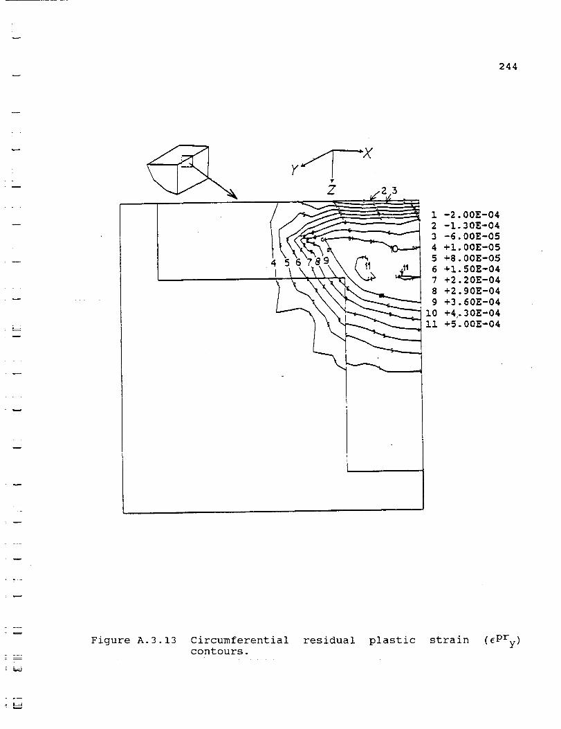
244

w

w

w

w

Z 23

1 -2.00E-04

2 -1.30E-04

3 -6.00E-05

4 +i. 00E-05

I 6 +1.50E-04• 7 +2.20E-04

8 +2.90E-04

9 +3.60E-04

I0 +4.30E-04II +5.00E-04

i

Figure A.3.13 Circumferential

contours.residual plastic strain (£pry)

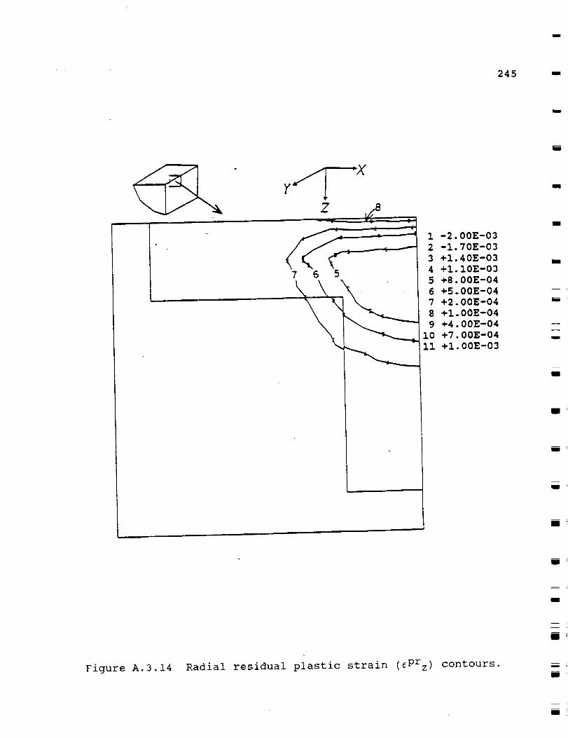
245

Z _8 _ 0

\\5

I -2.00E-03

2 -1.70E-03

3 +1.40E-03

4 +l.10E-03

5 +8.00E-04

6 +5.00E-04

7 +2.00E-04

8 +I.00E-04

9 +4.00E-04

i0 +7.00E-04

ii +I.00E-03

mm

at

i

Figure A.3.14 Radial residual plastic strain (6Prz) contours.

i

g

g

L

246

=

__ _ :

1 -2.00E-04

2 -i. 60E-04

3 -i. 20E-04

4 -8.00E-05

5 -4.00E-05

6 -2.81E-18

7 +4.00E-05

8 +8.00E-05

9 +1.20E-04

10 +1.60E-04

Ii +2.00E-04

Figure A.3.15 Residual shear plastic strain (_Prxy) contours.

247

Z

4

I -I.00E-032 -7.00E-043 +4.00E-04

4 +l. 00E-04

5 +2.00E-046 +5.00E-04

7 +8.00E-04

8 +i. 10E-03

9 +1.40E-03

i0 +1.70E-03

ii +2.00E-03

i__

m_

I

m [

Figure A.3.16Residual shear plastic strain (_Prxz) contours.

m_