c©Copyright 2014

Huy V. Tran

The regularity of Loewner curves

Huy V. Tran

A dissertation submitted in partial fulfillment of therequirements for the degree of

Doctor of Philosophy

University of Washington

2014

Reading Committee:

Steffen Rohde, Chair

Donald E. Marshall

Boris Solomyak

Program Authorized to Offer Degree:Mathematics

University of Washington

Abstract

The regularity of Loewner curves

Huy V. Tran

Chair of the Supervisory Committee:Professor Steffen Rohde

Mathematics

The Loewner differential equation, a classical tool that has attracted recent attention due

to Schramm-Loewner evolution (SLE), provides a unique way of encoding a simple 2-

dimensional curve into a continuous 1-dimensional driving function. In this thesis we study

the curve in three cases according to the regularity of driving function: weakly Holder-1/2,

Holder-1/2 with norm less than 4 and Cα with α ∈ (1/2,∞). In the first case, given the

existence of the curve we show that the standard algorithm simulating the curve converges

in a strong sense. One direct application is for simulating SLE. In the second case, we

give another proof of Marshall, Rohde [26] and Lind[22] in which the curve exists and is a

quasi-arc. A sufficient condition for the rectifiability of the curve is also given. In the final

case, we show that the Loewner curve is in Cα+1/2. The thesis is a combination of three

projects [39], [32] and [21] which are joint work with Joan Lind, Steffen Rohde and Michel

Zinsmeister.

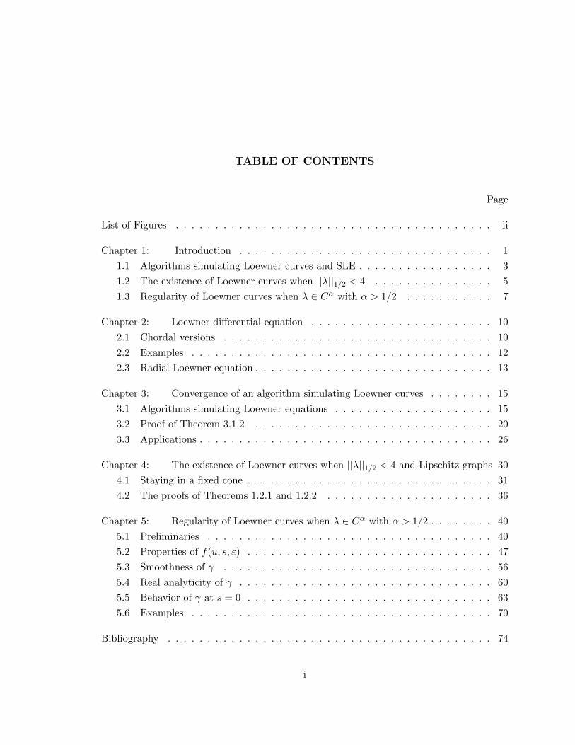
TABLE OF CONTENTS

Page

List of Figures . . . . . . . . . . . . . . . . . . . . . . . . . . . . . . . . . . . . . . . . ii

Chapter 1: Introduction . . . . . . . . . . . . . . . . . . . . . . . . . . . . . . . . 1

1.1 Algorithms simulating Loewner curves and SLE . . . . . . . . . . . . . . . . . 3

1.2 The existence of Loewner curves when ||λ||1/2 < 4 . . . . . . . . . . . . . . . 5

1.3 Regularity of Loewner curves when λ ∈ Cα with α > 1/2 . . . . . . . . . . . 7

Chapter 2: Loewner differential equation . . . . . . . . . . . . . . . . . . . . . . . 10

2.1 Chordal versions . . . . . . . . . . . . . . . . . . . . . . . . . . . . . . . . . . 10

2.2 Examples . . . . . . . . . . . . . . . . . . . . . . . . . . . . . . . . . . . . . . 12

2.3 Radial Loewner equation . . . . . . . . . . . . . . . . . . . . . . . . . . . . . . 13

Chapter 3: Convergence of an algorithm simulating Loewner curves . . . . . . . . 15

3.1 Algorithms simulating Loewner equations . . . . . . . . . . . . . . . . . . . . 15

3.2 Proof of Theorem 3.1.2 . . . . . . . . . . . . . . . . . . . . . . . . . . . . . . 20

3.3 Applications . . . . . . . . . . . . . . . . . . . . . . . . . . . . . . . . . . . . . 26

Chapter 4: The existence of Loewner curves when ||λ||1/2 < 4 and Lipschitz graphs 30

4.1 Staying in a fixed cone . . . . . . . . . . . . . . . . . . . . . . . . . . . . . . . 31

4.2 The proofs of Theorems 1.2.1 and 1.2.2 . . . . . . . . . . . . . . . . . . . . . 36

Chapter 5: Regularity of Loewner curves when λ ∈ Cα with α > 1/2 . . . . . . . . 40

5.1 Preliminaries . . . . . . . . . . . . . . . . . . . . . . . . . . . . . . . . . . . . 40

5.2 Properties of f(u, s, ε) . . . . . . . . . . . . . . . . . . . . . . . . . . . . . . . 47

5.3 Smoothness of γ . . . . . . . . . . . . . . . . . . . . . . . . . . . . . . . . . . 56

5.4 Real analyticity of γ . . . . . . . . . . . . . . . . . . . . . . . . . . . . . . . . 60

5.5 Behavior of γ at s = 0 . . . . . . . . . . . . . . . . . . . . . . . . . . . . . . . 63

5.6 Examples . . . . . . . . . . . . . . . . . . . . . . . . . . . . . . . . . . . . . . 70

Bibliography . . . . . . . . . . . . . . . . . . . . . . . . . . . . . . . . . . . . . . . . . 74

i

LIST OF FIGURES

Figure Number Page

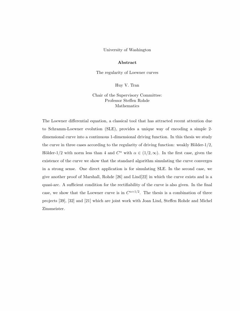
1.1 Illustration for SLE curves. See Figure 1.2 for simulations of the case κ = 8/3and κ = 6 . . . . . . . . . . . . . . . . . . . . . . . . . . . . . . . . . . . . . . 2

1.2 Simulations of SLE8/3 (left) and SLE6 (right) from the same Brownian motionsample with 12800 points . . . . . . . . . . . . . . . . . . . . . . . . . . . . . 4

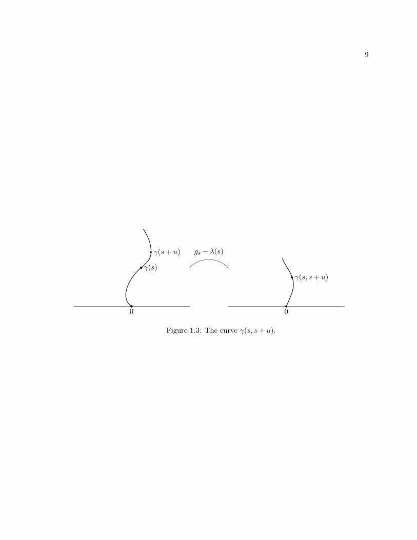
1.3 The curve γ(s, s+ u). . . . . . . . . . . . . . . . . . . . . . . . . . . . . . . . 9

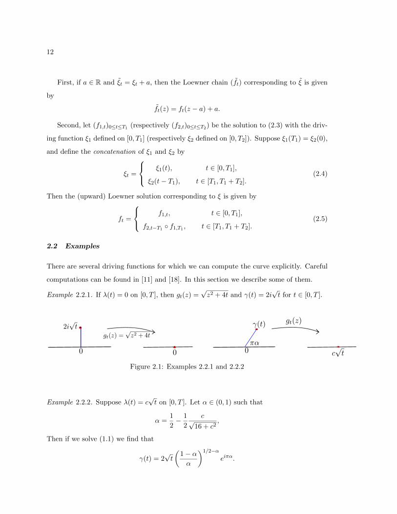
2.1 Examples 2.2.1 and 2.2.2 . . . . . . . . . . . . . . . . . . . . . . . . . . . . . . 12

2.2 Chordal Loewner chain (left) and radial Loewner chain . . . . . . . . . . . . . 14

3.1 At each step k, we compute Gnk , fntk and γntk . The k-th sub-arc of the simu-

lation curve γn is the image of γntk under fntk . . . . . . . . . . . . . . . . . . . 16

4.1 A trajectory of xt + iyt. It never leaves the cone Ac once outside AK . . . . . 34

5.1 Illustration for the proof of Theorem 1.3.4 . . . . . . . . . . . . . . . . . . . . 64

5.2 The conformal maps φ, gt, gt, φt, the comparison curve γ, and λ. . . . . . . . 67

5.3 Conformal maps used in the construction of γ for Example 1. . . . . . . . . . 71

5.4 The curve γ for Example 2. . . . . . . . . . . . . . . . . . . . . . . . . . . . 73

ii

ACKNOWLEDGMENTS

First of all I would like to thank everybody whom I have met, discussed or interact with

during my time as a graduate student. I have received advice, help, inspiration and learned

things from many people to become a better mathematician and person.

I am very thankful to Professor Michel Zinsmeister who met me many years ago in

Vietnam. It was my first time speaking English with a (mathematician) foreigner and I

was amazed how friendly and humorous he is. My interest in complex analysis came from

him and I have became his student since then. I appreciated his hospitality during my time

in France when he brought me to interesting conferences and seminars where I saw many

famous mathematicians that I had known from textbooks.

I wish to thank my advisor, Professor Steffen Rohde, for countless hours teaching and

guiding me. He is like my father, my counselor. Many times I walked into his office with just

one or two questions and a miserable feeling about the progress of my work. After hours of

discussion I left with more questions but gaining more confidence and with the hope that

things would work out as long as I kept working. I always enjoy having discussions with

him.

My coauthors Joan Lind, Steffen Rohde, Michel Zinsmeister all played essential parts

in the research behind this thesis. I owe thanks to Don Marshall, Elliot Paquette, Fredrik

Johansson Viklund, Brent Werness for carefully proofreading many parts in this thesis. If

the reader find any mistakes here, that’s the author’s fault.

During my time as a graduate student I had the privilege of attending the Interaction

between Analysis and Geometry programme at the Institute for Pure and Applied Math-

ematics (IPAM) at UCLA in Los Angeles. My joint work with Joan Lind started when I

was there. I most gratefully acknowledge the support of this institution.

I wish also to thank Professors Zhen-Qing Chen, Mathias Drton, Donald Marshall,

iii

Steffen Rohde, Boris Solomyak for serving on my supervisory committee.

Finally, I would like to thank my family: my father and mother, my wife Linh Tran, for

their continuous, invaluable, and essential support.

iv

DEDICATION

To my parents, my wife Linh Tran, and my son Tien-Minh (Oscar)

v

1

Chapter 1

INTRODUCTION

The chordal Loewner differential equation in the upper half plane H

∂tgt(z) =2

gt(z)− λt, g0(z) = z, (1.1)

which will be reviewed in Chapter 2, provides a one-to-one correspondence between certain

decreasing families of simply connected subdomains H\Kt of the upper half plane, and real-

valued continuous functions λt. Initially developed as a tool to study extremal problems

in complex analysis [24], it has become an important tool in probability theory, based on

Oded Schramm’s insight [33] that Brownian motion arises naturally as the driving function

λt in various settings of random sets Kt.

Consider triples (Ω, a, b) with a simply connected domain Ω and two marked points a, b

on the boundary. Suppose that for each triple (Ω, a, b), we consider a random continuous

curve γ(Ω,a,b) that goes from a to b in Ω. If ∂Ω is not locally connected, we consider a and

b to be prime ends. In this case, the curve γΩ,a,b is the image of a continuous curve going

from -1 to 1 in D under a conformal φ : D→ Ω that sends a and b to -1 and 1 respectively.

Definition 1.0.1. We say that the family of random continuous curves γ(Ω,a,b) is confor-

mally invariant if for any (Ω, a, b) and any conformal map φ : Ω→ C ,

φ γ(Ω,a,b) has the same law as φ(φ(Ω),φ(a),φ(b)).

Definition 1.0.2. We say that the family of random continuous curves γ(Ω,a,b) satisfies

the domain Markov property if for every (Ω, a, b), and every t > 0, the law of the curve

γ[t,∞) conditionally on γ[0, t] is the same as the law of γ(Ωt,γt,b), where Ωt is the connected

component of Ω\γt containing b in its boundary.

In 1999, Schramm introduced a one-parameter family SLEκ with κ ≥ 0 of measures that

satisfy the conformal invariance and Markov domain property. This family of measures

2

is a candidate for the scaling limits of many discrete models in statistical physics. When

translated in the upper half-plane H, the SLEκ is the solution to (1.1) with λt =√κBt,

where Bt is a standard Brownian motion. And thanks to this connection to Brownian

motion, SLE can be studied via standard techniques such as stochastic calculus. The SLEκ

is almost surely a curve1 for all κ ≥ 0 ([31], [17]) and it exhibits phase transitions:

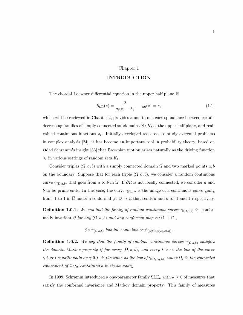
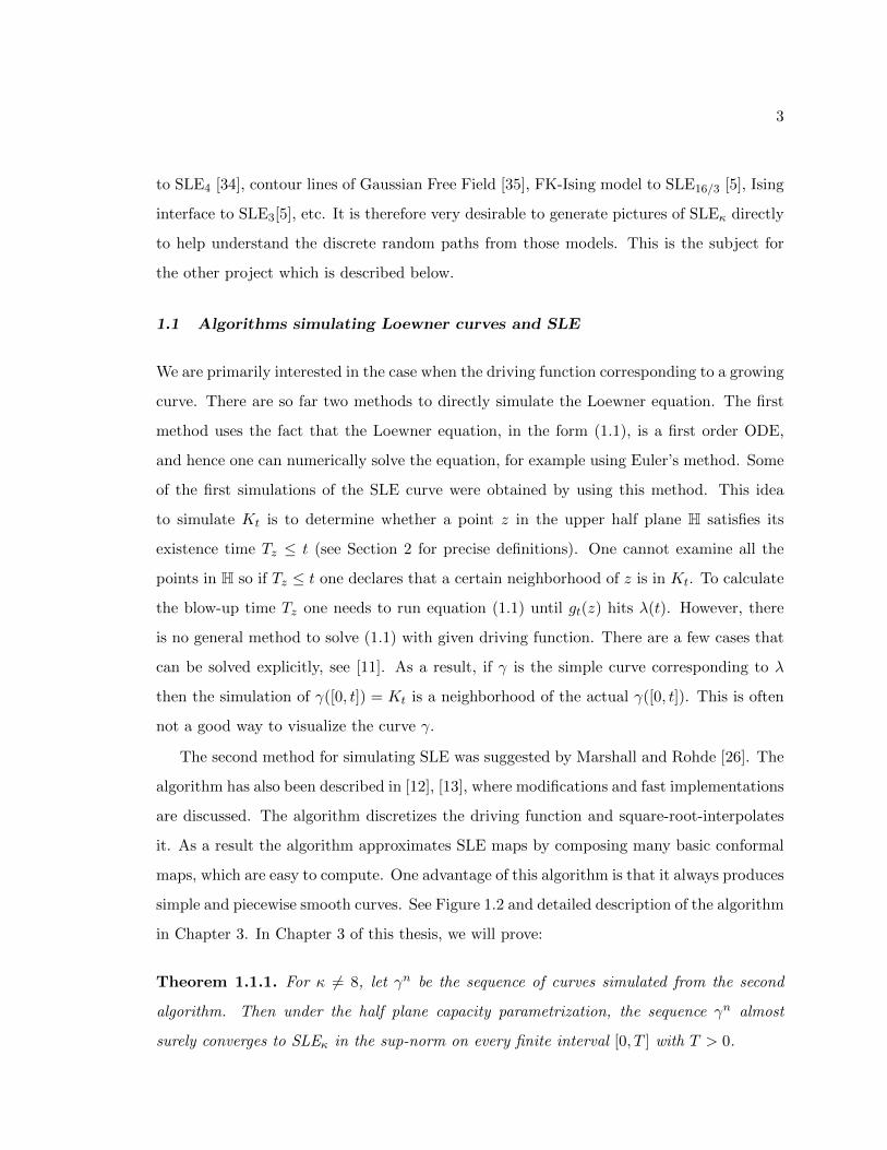
• For κ ∈ [0, 4], SLEκ is almost surely a simple path contained in H ∪ 0.

• For κ ∈ (4, 8), SLEκ is almost surely a non-simple path.

• For κ ≥ 8, SLEκ is almost surely a space-filling curve.

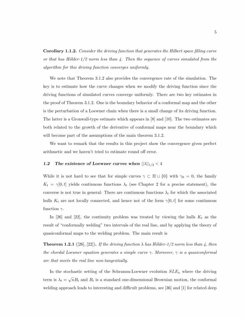
Figure 1.1: Illustration for SLE curves. See Figure 1.2 for simulations of the case κ = 8/3

and κ = 6

Its fractal behavior is also known such as Hausdorff dimension [3], Minkowski dimension

[30], best Holder exponent [9] [23], etc.

There are not many studies of the same questions in the deterministic setting, i.e., the

Loewner equation with general deterministic driving function. Two projects in this thesis

investigate the regularity of the curve given that of the driving function. See Sections 1.2

1.3 in this introductory chapter.

Many models are known to converge to SLE such as interfaces of site percolation on the

triangular lattice to SLE6 [38], loop-erased random walks to SLE2 [17], harmonic explorer

1In other words it is a measure supported on curves.

3

to SLE4 [34], contour lines of Gaussian Free Field [35], FK-Ising model to SLE16/3 [5], Ising

interface to SLE3[5], etc. It is therefore very desirable to generate pictures of SLEκ directly

to help understand the discrete random paths from those models. This is the subject for

the other project which is described below.

1.1 Algorithms simulating Loewner curves and SLE

We are primarily interested in the case when the driving function corresponding to a growing

curve. There are so far two methods to directly simulate the Loewner equation. The first

method uses the fact that the Loewner equation, in the form (1.1), is a first order ODE,

and hence one can numerically solve the equation, for example using Euler’s method. Some

of the first simulations of the SLE curve were obtained by using this method. This idea

to simulate Kt is to determine whether a point z in the upper half plane H satisfies its

existence time Tz ≤ t (see Section 2 for precise definitions). One cannot examine all the

points in H so if Tz ≤ t one declares that a certain neighborhood of z is in Kt. To calculate

the blow-up time Tz one needs to run equation (1.1) until gt(z) hits λ(t). However, there

is no general method to solve (1.1) with given driving function. There are a few cases that

can be solved explicitly, see [11]. As a result, if γ is the simple curve corresponding to λ

then the simulation of γ([0, t]) = Kt is a neighborhood of the actual γ([0, t]). This is often

not a good way to visualize the curve γ.

The second method for simulating SLE was suggested by Marshall and Rohde [26]. The

algorithm has also been described in [12], [13], where modifications and fast implementations

are discussed. The algorithm discretizes the driving function and square-root-interpolates

it. As a result the algorithm approximates SLE maps by composing many basic conformal

maps, which are easy to compute. One advantage of this algorithm is that it always produces

simple and piecewise smooth curves. See Figure 1.2 and detailed description of the algorithm

in Chapter 3. In Chapter 3 of this thesis, we will prove:

Theorem 1.1.1. For κ 6= 8, let γn be the sequence of curves simulated from the second

algorithm. Then under the half plane capacity parametrization, the sequence γn almost

surely converges to SLEκ in the sup-norm on every finite interval [0, T ] with T > 0.

4

−0.5 0 0.50

0.2

0.4

0.6

0.8

1

1.2

1.4

1.6

1.8

−1 −0.8 −0.6 −0.4 −0.2 0 0.2 0.4 0.6 0.80

0.2

0.4

0.6

0.8

1

1.2

1.4

1.6

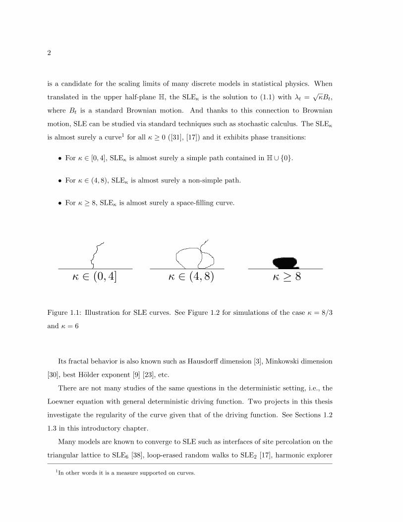
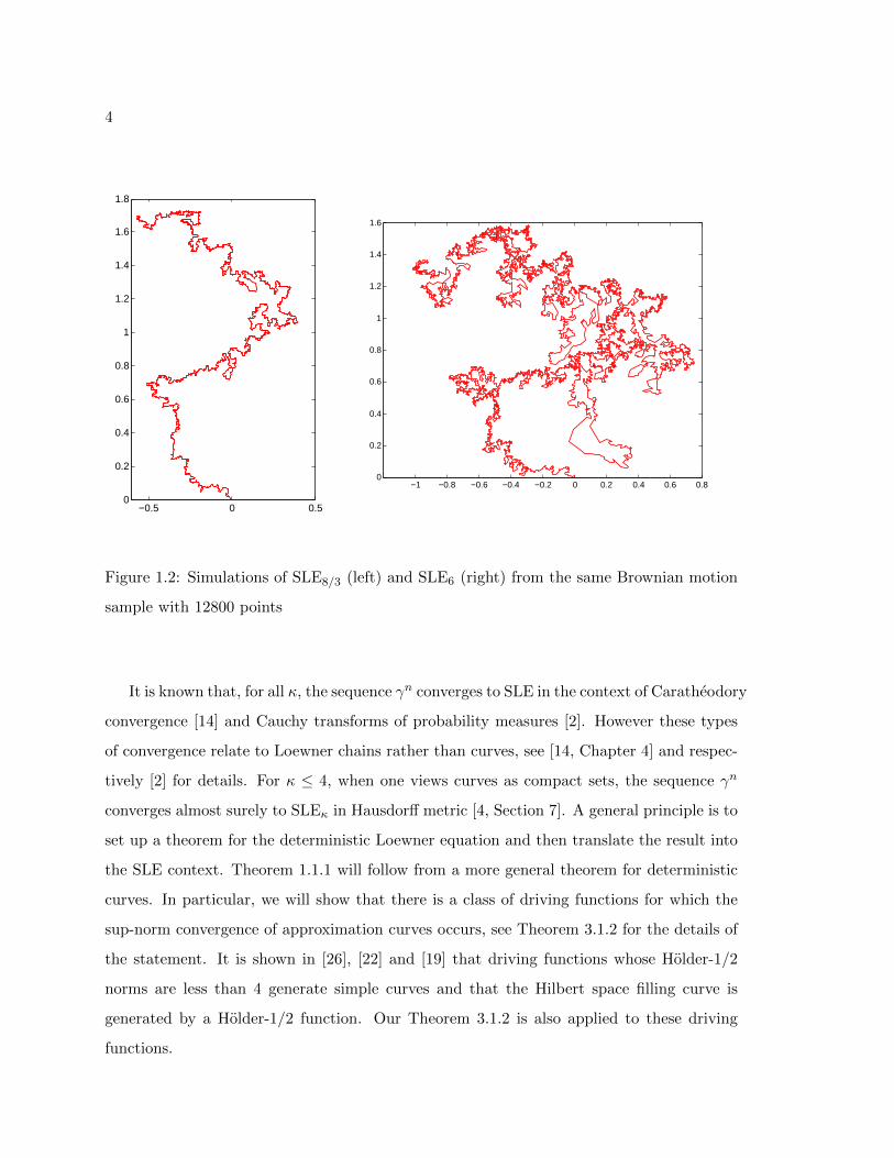
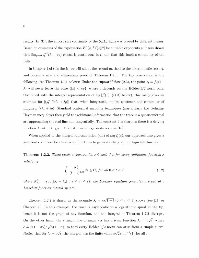
Figure 1.2: Simulations of SLE8/3 (left) and SLE6 (right) from the same Brownian motion

sample with 12800 points

It is known that, for all κ, the sequence γn converges to SLE in the context of Caratheodory

convergence [14] and Cauchy transforms of probability measures [2]. However these types

of convergence relate to Loewner chains rather than curves, see [14, Chapter 4] and respec-

tively [2] for details. For κ ≤ 4, when one views curves as compact sets, the sequence γn

converges almost surely to SLEκ in Hausdorff metric [4, Section 7]. A general principle is to

set up a theorem for the deterministic Loewner equation and then translate the result into

the SLE context. Theorem 1.1.1 will follow from a more general theorem for deterministic

curves. In particular, we will show that there is a class of driving functions for which the

sup-norm convergence of approximation curves occurs, see Theorem 3.1.2 for the details of

the statement. It is shown in [26], [22] and [19] that driving functions whose Holder-1/2

norms are less than 4 generate simple curves and that the Hilbert space filling curve is

generated by a Holder-1/2 function. Our Theorem 3.1.2 is also applied to these driving

functions.

5

Corollary 1.1.2. Consider the driving function that generates the Hilbert space filling curve

or that has Holder-1/2 norm less than 4. Then the sequence of curves simulated from the

algorithm for this driving function converges uniformly.

We note that Theorem 3.1.2 also provides the convergence rate of the simulation. The

key is to estimate how the curve changes when we modify the driving function since the

driving functions of simulated curves converge uniformly. There are two key estimates in

the proof of Theorem 3.1.2. One is the boundary behavior of a conformal map and the other

is the perturbation of a Loewner chain when there is a small change of its driving function.

The latter is a Gronwall-type estimate which appears in [8] and [10]. The two estimates are

both related to the growth of the derivative of conformal maps near the boundary which

will become part of the assumptions of the main theorem 3.1.2.

We want to remark that the results in this project show the convergence given perfect

arithmetic and we haven’t tried to estimate round off error.

1.2 The existence of Loewner curves when ||λ||1/2 < 4

While it is not hard to see that for simple curves γ ⊂ H ∪ 0 with γ0 = 0, the family

Kt = γ[0, t] yields continuous functions λt (see Chapter 2 for a precise statement), the

converse is not true in general: There are continuous functions λt for which the associated

hulls Kt are not locally connected, and hence not of the form γ[0, t] for some continuous

function γ.

In [26] and [22], the continuity problem was treated by viewing the hulls Kt as the

result of “conformally welding” two intervals of the real line, and by applying the theory of

quasiconformal maps to the welding problem. The main result is

Theorem 1.2.1 ([26], [22]). If the driving function λ has Holder-1/2 norm less than 4, then

the chordal Loewner equation generates a simple curve γ. Moreover, γ is a quasiconformal

arc that meets the real line non-tangentially.

In the stochastic setting of the Schramm-Loewner evolution SLEκ where the driving

term is λt =√κBt and Bt is a standard one-dimensional Brownian motion, the conformal

welding approach leads to interesting and difficult problems, see [36] and [1] for related deep

6

results. In [31], the almost sure continuity of the SLEκ hulls was proved by different means:

Based on estimates of the expectation E[|(g−1t )′(z)|p] for suitable exponents p, it was shown

that limy→0 g−1t (λt + iy) exists, is continuous in t, and that this implies continuity of the

hulls.

In Chapter 4 of this thesis, we will adopt the second method to the deterministic setting,

and obtain a new and elementary proof of Theorem 1.2.1. The key observation is the

following (see Theorem 4.1.1 below): Under the “upward” flow (2.3), the point zt = ft(i)−

λt will never leave the cone |x| < cy, where c depends on the Holder-1/2 norm only.

Combined with the integral representation of log |f ′t(z)| ((4.3) below), this easily gives an

estimate for |(g−1t )′(λt + iy)| that, when integrated, implies existence and continuity of

limy→0 g−1t (λt + iy). Standard conformal mapping techniques (particularly the Gehring-

Hayman inequality) then yield the additional information that the trace is a quasiconformal

arc approaching the real line non-tangentially. The constant 4 is sharp as there is a driving

function λ with ||λ||1/2 = 4 but it does not generate a curve [18].

When applied to the integral representation (4.4) of arg f ′t(z), our approach also gives a

sufficient condition for the driving functions to generate the graph of Lipschitz function:

Theorem 1.2.2. There exists a constant C0 > 0 such that for every continuous function λ

satisfying ∫ t

0

Nλs,t

(t− s)3/2ds ≤ C0 for all 0 < t < T (1.2)

where Nλs,t = sup|λr − λs| : s ≤ r ≤ t, the Loewner equation generates a graph of a

Lipschitz function rotated by 90o.

Theorem 1.2.2 is sharp, as the example λt = c√

1− t (0 ≤ t ≤ 1) shows (see [11] or

Chapter 2). In this example, the trace is asymptotic to a logarithmic spiral at the tip,

hence it is not the graph of any function, and the integral in Theorem 1.2.2 diverges.

On the other hand, the straight line of angle πα has driving function λt = c√t, where

c = 2(1 − 2α)/√α(1− α), so that every Holder-1/2 norm can arise from a simple curve.

Notice that for λt = c√t, the integral has the finite value c

√2 sinh−1(1) for all t.

7

1.3 Regularity of Loewner curves when λ ∈ Cα with α > 1/2

It is natural to ask how properties of the Loewner curve γ correspond to properties of the

driving function λ. In Chapter 5 of this paper, we prove the following theorem relating the

regularity of λ to the regularity of γ.

Theorem 1.3.1. Let λ ∈ Cβ[0, T ] for β > 2. Then the Loewner curve γ is Cβ+ 12 (0, T ],

provided that β + 1/2 /∈ N.

See Theorem 5.3.1 for a quantitative version. Theorem 1.3.1 extends the work in [40],

where the result was proven for β ∈ (1/2, 2]. In Section 5.6, we discuss an example where

λ ∈ C3/2 but γ fails to be C2, showing that it is not possible to strengthen Theorem 1.3.1

to say that γ ∈ Cn+1 when λ ∈ Cn+1/2. We also address the analytic case:

Theorem 1.3.2. If λ is real analytic on [0, T ], then γ is also real analytic on (0, T ].

Notice that in both of these theorems, the regularity of γ is on the time interval (0, T ].

With the halfplane-capacity parametrization, it is not possible to extend these results to

t = 0. To see this, consider the example when the driving function is λ(t) ≡ 0. Then

the corresponding Loewner curve is γ(t) = 2i√t. Further, with the halfplane-capacity

parametrization, γ(t) can always be expanded at t = 0 in powers of√t, as we see in the

following theorem.

Theorem 1.3.3. Assume that λ ∈ Cn+α[0, T ] for n ∈ N and α ∈ (0, 1]. Then near t = 0,

γ(t) =

2i√t+ a2t+ i a3t

3/2 + a4t2 + · · ·+ a2nt

n +O(tn+α) if α ≤ 1/2

2i√t+ a2t+ i a3t

3/2 + a4t2 + · · ·+ a2nt

n + i a2n+1tn+1/2 +O(tn+α) if α > 1/2

where the real-valued coefficients am depend on λ(k)(0) for k = 1, · · · , bm2 c.

If we make the simple change of parametrization t = s2, then the smoothness extends

to s = 0.

Theorem 1.3.4. Let Γ(s) = γ(s2) be the reparametrized Loewner curve with driving func-

tion λ. If λ is real analytic on [0, T ], then Γ is real analytic on [0,√T ]. If λ ∈ Cβ[0, T ],

then curve Γ ∈ Cβ+1/2[0,√T ] when β + 1/2 /∈ N.

8

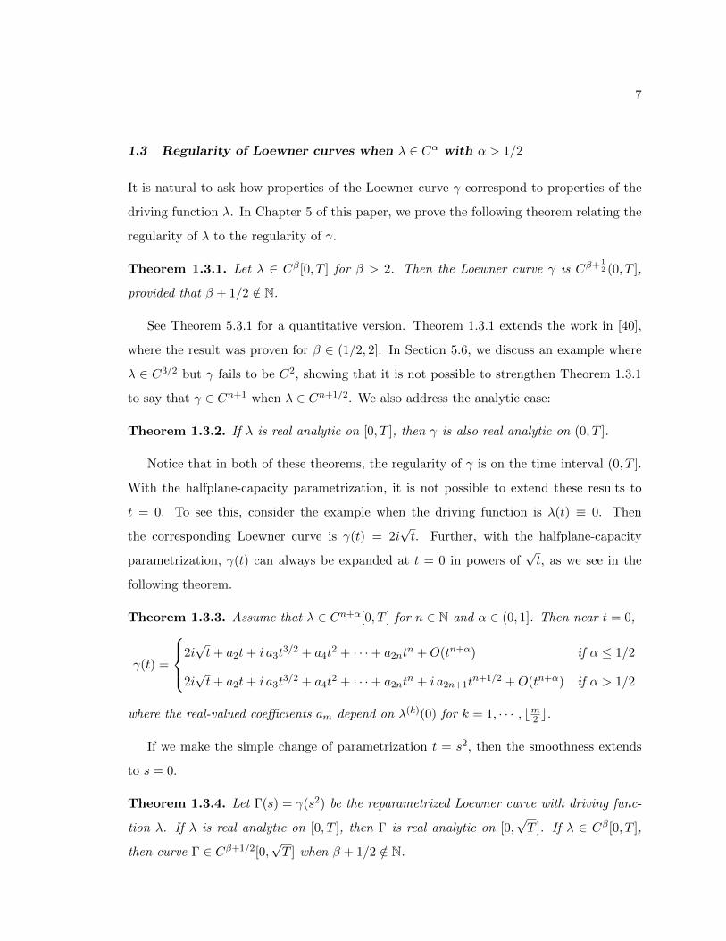
We wish to briefly describe the key tool used in Chapter 5. For s ∈ [0, T ], consider the

simple curve gs(γ(s+u))−λ(s), which we denote by γ(s, s+u), 0 ≤ u ≤ T−s. See Figure 1.3.

The curve γ(s, s+u) corresponds to the time-shifted driving function λs(u) = λ(u+s)−λ(s),

0 ≤ u ≤ T − s. It follows from [40, Theorem 6.2] that under the assumption λ ∈ C2([0, T ]),

the curve γ is in C2 and

γ′′(s) =2γ′(s)

γ(s)2− 4γ′(s)

∫ s

0

∂s[γ(s− u, s)]γ(s− u, s)3

du. (1.3)

In order to understand the higher differentiability of γ, we need to understand γ(s− u, s).

Differentiating this function with respect to u, we obtain

∂u[γ(s− u, s)] = ∂u[gs−u(γ(s))− λ(s− u)] =−2

γ(s− u, s)+ λ′(s− u) for 0 < u ≤ s, (1.4)

and γ(s − u, s)|u=0 = γ(s, s) = 0. We note that the above differential equation does not

hold for u = 0. This is the reason for us to investigate the following ODE:

f ′(u) =−2

f(u)+ λ′(s− u), 0 ≤ u ≤ s, (1.5)

f(0) = iε ∈ H.

The work in this project depends on a deep understanding of the function f(u) = f(u, s, ε)

which is the solution to (1.5). Once we show that f(u, s, ε) converges uniformly to γ(s−u, s)

as ε → 0+, we can use (1.3) to translate information about f into information about the

derivatives of γ.

Remark. Theorem 1.3.1 and Theorem 1.3.2 provide a converse to the results of Earle and

Epstein in [7]. Their results (translated from the radial setting to the chordal setting using

[25]) state that if any parametrization of γ is Cn, then the halfplane-capacity parametriza-

tion of γ is in Cn−1(0, T ) and λ ∈ Cn−1(0, T ). They also prove that if γ is real analytic,

then λ must be real analytic.

Organization. This thesis is split into four chapters after this one. In Chapter 2 we

review Loewner differential equation and give examples. The theorems in Sections 1.1, 1.2

and 1.3 are presented Chapter 3, 4 and 5, respectively.

9

γ(s)

γ(s+ u) gs − λ(s)

0 0

γ(s, s+ u)

Figure 1.3: The curve γ(s, s+ u).

10

Chapter 2

LOEWNER DIFFERENTIAL EQUATION

2.1 Chordal versions

There are many versions of the Loewner equation. The original version is radial Loewner

equation in the unit disk D. In this thesis we only focus on the chordal version in the upper

half plane H. This version is popular because of its simple form, which was introduced by

Schramm [33]. The radial case is introduced in Section 2.3. For more details we refer the

reader to [14].

Let γ : [0, T ] → H ∪ 0 be a simple curve in the upper half-plane H except that

γ0 ≡ γ(0) ∈ R1. For each t ∈ [0, T ], by the Riemann mapping theorem there exists a unique

conformal map gt : H\γ[0, t]→ H satisfying the hydrodynamic normalization:

gt(z) = z +ctz

+ · · · when z →∞.

It can be shown that ct is a nonnegative, strictly increasing, continuous function and c0 = 0

[14]. Hence one can reparametrize γ according to half-plane capacity, which means ct = 2t.

Then for each z ∈ H, the function t 7→ gt(z) satisfies the (downward) chordal Loewner

equation:

∂tgt(z) =2

gt(z)− λt, g0(z) = z, (2.1)

where λ is a continuous, real-valued function and gt(γt) = λt, see [14, Chapter 4].

Conversely, if one starts with a continuous function λ : [0, T ] → R, one can consider the

initial value problem for each z ∈ H:

∂tg(t, z) =2

g(t, z)− λt, g(0, z) = z.

For each z ∈ H there is a maximal interval for which a solution g(t, z) exists. Let Tz =

1In this thesis, when writing functions of variable t, we usually let t be a subscript.

11

sups ∈ [0, T ] : g(t, z) exists on [0, s). It is easy to see that, if Tz < T , then

limt→Tz

g(t, z) = λ(Tz).

Let Ht = z ∈ H : Tz > t and gt(z) = g(t, z). Then one can show that the set Ht is simply

connected subdomain of H and gt(z) is the unique conformal map from Ht onto H with the

following normalization near infinity:

gt(z) = z +2t

z+O

(1

z2

).

The driving function λ of the Loewner chain (gt) is said to generate a curve if there exists

a curve γ such that Ht is the unbounded component of H\γ[0, t] for each t ≥ 0. By [31,

Theorem 4.1], this is equivalent to the existence and continuity in t > 0 of

γt := limy→0+

g−1t (λt + iy). (2.2)

By [15, Proposition 2.19] and [9, Proposition 3.11], a very useful and simple criterion for

this existence and continuity is the convergence to zero of

v(t, ε) :=

∫ ε

0|(g−1

t )′(λt + iy)|dy

as ε→ 0, uniformly in t ∈ [0, T ].

Rather than directly working with the Loewner equation (1.1), it is often easier to work

with the upward Loewner equation:

∂tft(z) =−2

ft(z)− ξt, f0(z) = z, (2.3)

for z ∈ H and real-valued continuous function ξt. Since the imaginary part of ft(z) is strictly

increasing, the solution exists uniquely for all time t ≥ 0. If (gt)0≤t≤T is the solution to

(1.1) with driving function λ and if (ft)0≤t≤T is the solution to (2.3) with ξt = λT−t, then

ft(z) = gT−t(g−1T (z)) and in particular

fT (z) = g−1T (z).

We will frequently use the following two simple properties of the Loewner equation, regard-

ing the translation and concatenation of driving functions:

12

First, if a ∈ R and ξt = ξt + a, then the Loewner chain (ft) corresponding to ξ is given

by

ft(z) = ft(z − a) + a.

Second, let (f1,t)0≤t≤T1 (respectively (f2,t)0≤t≤T2) be the solution to (2.3) with the driv-

ing function ξ1 defined on [0, T1] (respectively ξ2 defined on [0, T2]). Suppose ξ1(T1) = ξ2(0),

and define the concatenation of ξ1 and ξ2 by

ξt =

ξ1(t), t ∈ [0, T1],

ξ2(t− T1), t ∈ [T1, T1 + T2].(2.4)

Then the (upward) Loewner solution corresponding to ξ is given by

ft =

f1,t, t ∈ [0, T1],

f2,t−T1 f1,T1 , t ∈ [T1, T1 + T2].(2.5)

2.2 Examples

There are several driving functions for which we can compute the curve explicitly. Careful

computations can be found in [11] and [18]. In this section we describe some of them.

Example 2.2.1. If λ(t) = 0 on [0, T ], then gt(z) =√z2 + 4t and γ(t) = 2i

√t for t ∈ [0, T ].

Figure 2.1: Examples 2.2.1 and 2.2.2

Example 2.2.2. Suppose λ(t) = c√t on [0, T ]. Let α ∈ (0, 1) such that

α =1

2− 1

2

c√16 + c2

,

Then if we solve (1.1) we find that

γ(t) = 2√t

(1− αα

)1/2−αeiπα.

13

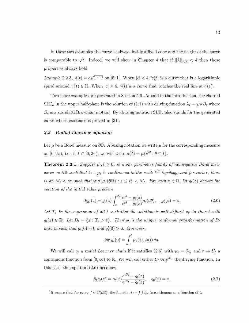
In these two examples the curve is always inside a fixed cone and the height of the curve

is comparable to√t. Indeed, we will show in Chapter 4 that if ||λ||1/2 < 4 then those

properties always hold.

Example 2.2.3. λ(t) = c√

1− t on [0, 1]. When |c| < 4, γ(t) is a curve that is a logarithmic

spiral around γ(1) ∈ H. When |c| ≥ 4, γ(t) is a curve that touches the real line at γ(1).

Two more examples are presented in Section 5.6. As said in the introduction, the chordal

SLEκ in the upper half-plane is the solution of (1.1) with driving function λt =√κBt where

Bt is a standard Brownian motion. By abusing notation SLEκ also stands for the generated

curve whose existence is proved in [31].

2.3 Radial Loewner equation

Let µ be a Borel measure on ∂D. Abusing notation we write µ for the corresponding measure

on [0, 2π), i.e., if I ⊂ [0, 2π), we will write µ(I) = µeiθ : θ ∈ I.

Theorem 2.3.1. Suppose µt, t ≥ 0, is a one parameter family of nonnegative Borel mea-

sures on ∂D such that t 7→ µt is continuous in the weak-* 2 topology, and for each t, there

is an Mt < ∞ such that supµs(∂D) : s ≤ t < Mt. For each z ∈ D, let gt(z) denote the

solution of the initial value problem

∂tgt(z) = gt(z)

∫ 2π

0

eiθ + gt(z)

eiθ − gt(z)µt(dθ), g0(z) = z. (2.6)

Let Tz be the supremum of all t such that the solution is well defined up to time t with

gt(z) ∈ D. Let Dt = z : Tz > t. Then gt is the unique conformal transformation of Dt

onto D such that gt(0) = 0 and g′t(0) > 0. Moreover,

log g′t(0) =

∫ t

0µs([0, 2π)) ds.

We will call gt a radial Loewner chain if it satisfies (2.6) with µt = δUt and t 7→ Ut a

continuous function from [0,∞) to R. We will call either Ut or eiUt the driving function. In

this case, the equation (2.6) becomes

∂tgt(z) = gt(z)eiUt + gt(z)

eiUt − gt(z), g0(z) = z. (2.7)

2It means that for every f ∈ C(∂D), the function t 7→∫fdµt is continuous as a function of t.

14

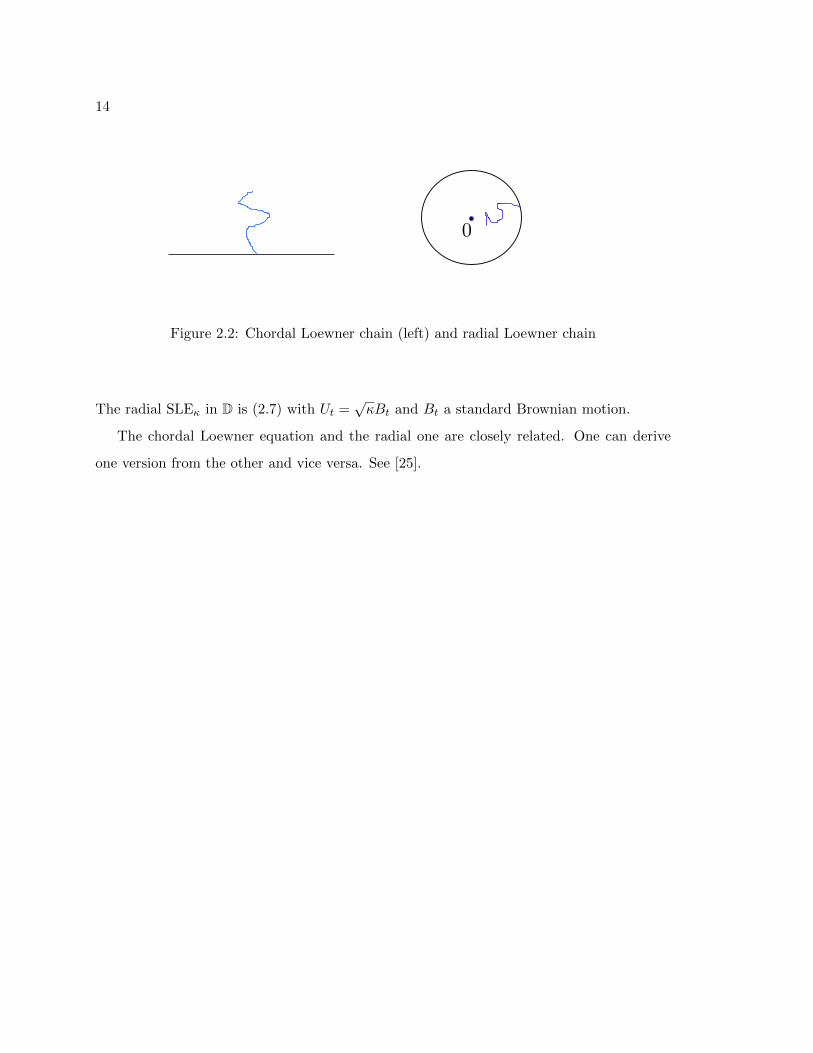
Figure 2.2: Chordal Loewner chain (left) and radial Loewner chain

The radial SLEκ in D is (2.7) with Ut =√κBt and Bt a standard Brownian motion.

The chordal Loewner equation and the radial one are closely related. One can derive

one version from the other and vice versa. See [25].

15

Chapter 3

CONVERGENCE OF AN ALGORITHM SIMULATING LOEWNERCURVES

3.1 Algorithms simulating Loewner equations

We now discuss in more detail the algorithm to simulate Loewner curves. The algorithm

is based on two observations. First, fix s > 0, and let (gt) be the solution of the Loewner

equation with driving function λ(t) = λ(s + t), t ≥ 0. This solution can be obtained by

gs+t g−1s . Indeed

∂tgs+t g−1s (z) =

2

gs+t g−1s (z)− λ(s+ t)

=2

gs+t g−1s (z)− λ(t)

,

and gsg−1s (z) = z. By the uniqueness of solution of the equation (1.1), gt(z) = gs+tg−1

s (z).

If we let Kt be the hull associated with gt then

gs(Ks+t) = Kt and Ks+t = Ks ∪ g−1s (Kt).

So in order to compute Ks+t, one can compute Ks and g−1s , by using the information of λ

on [0, s], and compute Kt by using λ on [s, s+ t].

The second observation is that when λ is of the form c√t+ d, for some real constants c

and d, one can solve for Kt explicitly. In this case, Kt is a segment in the upper half plane

starting at d ∈ R that makes an angle απ with the positive real axis where

α =1

2− 1

2

c√16 + c2

,

and g−1t (z + λ(t)) = (z + 2

√t√

α1−α)1−α(z − 2

√t√

α1−α)α + d. See [11] for a proof.

We now fix a step n ≥ 1. Let tk = kn for 0 ≤ k ≤ n. So t0 = 0, t1, · · · , tn = 1 is a partition

of [0, 1]. We will solve the Loewner equation with driving functions λ(t+ tk) for 0 ≤ t ≤ 1n .

By the remarks above, one should approximate these driving functions by c√t+ d so that

one can solve explicitly the Loewner equation. More specifically, we approximate λ by λn

16

such that they attain the same values at tk’s and that λn is a scaling and translation of√t

on [tk, tk+1] from λ(tk) to λ(tk+1). Hence the function λn is defined as follows:

λn(t) =√n(λ(tk+1)− λ(tk))

√t− tk + λ(tk) on [tk, tk+1].

This driving function always produces a simple curve γn : [0, 1]→ H ∪ λ(0).

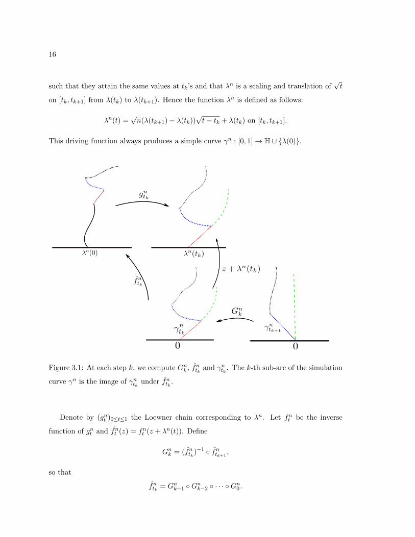
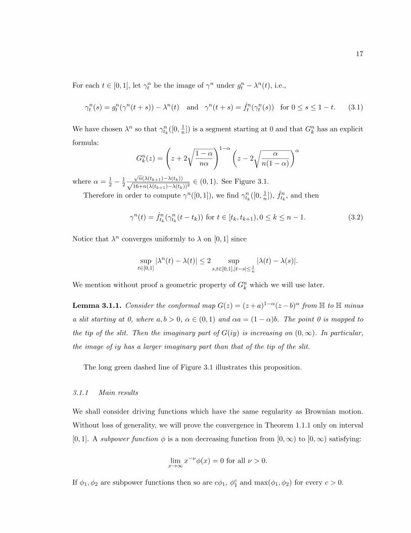
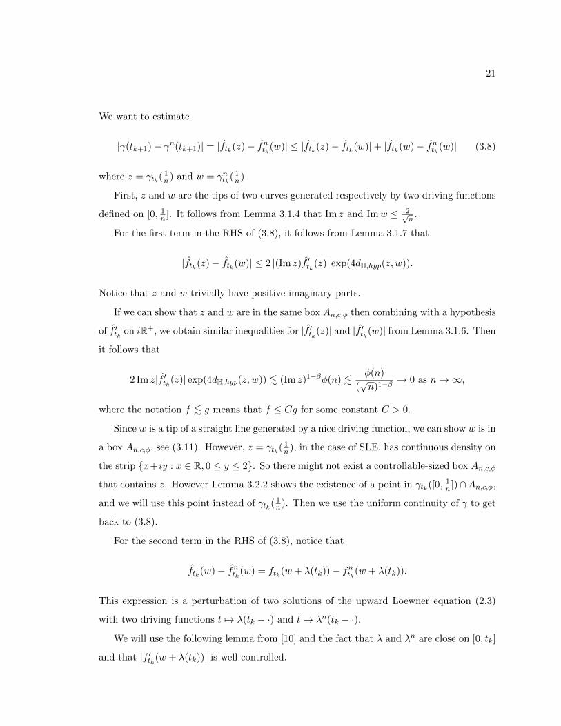
Figure 3.1: At each step k, we compute Gnk , fntk and γntk . The k-th sub-arc of the simulation

curve γn is the image of γntk under fntk .

Denote by (gnt )0≤t≤1 the Loewner chain corresponding to λn. Let fnt be the inverse

function of gnt and fnt (z) = fnt (z + λn(t)). Define

Gnk = (fntk)−1 fntk+1,

so that

fntk = Gnk−1 Gnk−2 · · · Gn0 .

17

For each t ∈ [0, 1], let γnt be the image of γn under gnt − λn(t), i.e.,

γnt (s) = gnt (γn(t+ s))− λn(t) and γn(t+ s) = fnt (γnt (s)) for 0 ≤ s ≤ 1− t. (3.1)

We have chosen λn so that γntk([0, 1n ]) is a segment starting at 0 and that Gnk has an explicit

formula:

Gnk(z) =

(z + 2

√1− αnα

)1−α(z − 2

√α

n(1− α)

)αwhere α = 1

2 −12

√n(λ(tk+1)−λ(tk))√

16+n(λ(tk+1)−λ(tk))2∈ (0, 1). See Figure 3.1.

Therefore in order to compute γn([0, 1]), we find γntk([0, 1n ]), fntk , and then

γn(t) = fntk(γntk(t− tk)) for t ∈ [tk, tk+1), 0 ≤ k ≤ n− 1. (3.2)

Notice that λn converges uniformly to λ on [0, 1] since

supt∈[0,1]

|λn(t)− λ(t)| ≤ 2 sups,t∈[0,1],|t−s|≤ 1

n

|λ(t)− λ(s)|.

We mention without proof a geometric property of Gnk which we will use later.

Lemma 3.1.1. Consider the conformal map G(z) = (z+a)1−α(z− b)α from H to H minus

a slit starting at 0, where a, b > 0, α ∈ (0, 1) and αa = (1− α)b. The point 0 is mapped to

the tip of the slit. Then the imaginary part of G(iy) is increasing on (0,∞). In particular,

the image of iy has a larger imaginary part than that of the tip of the slit.

The long green dashed line of Figure 3.1 illustrates this proposition.

3.1.1 Main results

We shall consider driving functions which have the same regularity as Brownian motion.

Without loss of generality, we will prove the convergence in Theorem 1.1.1 only on interval

[0, 1]. A subpower function φ is a non decreasing function from [0,∞) to [0,∞) satisfying:

limx→∞

x−νφ(x) = 0 for all ν > 0.

If φ1, φ2 are subpower functions then so are cφ1, φc1 and max(φ1, φ2) for every c > 0.

18

The function λ is called weakly Holder-1/2 if there exists a subpower function ϕ such

that

osc(λ; δ) := sup|λ(t)− λ(s)| : s, t ∈ [0, 1], |t− s| ≤ δ ≤√δϕ(1/δ) for all δ > 0. (3.3)

It follows from P.Levy’s theorem that the sample paths of Brownian motion are almost

surely weakly Holder-1/2 with subpower function c√

log(δ), c >√

2, see [29, Theorem

I.2.7].

It is known that if λ is weakly Holder-1/2 and if there exist c0 > 0, y0 > 0 and 0 < β < 1

so that

|f ′t(iy)| ≤ c0y−β for all 0 < y ≤ y0, t ∈ [0, 1], (3.4)

where ft(·) = g−1t (λ(t) + ·), then (gt)0≤t≤1 is generated by a curve, see [9, section 3]. This

is one of the main ideas to show the existence of SLE curves for κ 6= 8 ([31]). We note that

the Loewner chain of SLE8 does not satisfy (3.4).

Our main theorem shows that under these hypotheses the algorithm gives the sup-norm

convergence of the simulation curves.

Theorem 3.1.2. Suppose λ is a weakly Holder-1/2 driving function with a subpower func-

tion ϕ and suppose the condition (3.4) is satisfied. Then the curve γ generated from the

Loewner equation can be approximated by the algorithm; that is, there exists a subpower

function ϕ such that for all n ≥ 1y20

and t ∈ [0, 1],

|γn(t)− γ(t)| ≤ ϕ(n)

n12

(1−√

1+β2

), (3.5)

where γn is the curve generated from the algorithm which is explained in section 3.1. The

function ϕ depends on ϕ, c0 and β.

A related question is the following: under what additional assumptions, does the uniform

convergence of driving functions imply convergence of corresponding curves? A priori the

convergence of curves occurs in the sense of Caratheodory convergence, see [14], and in the

sense of Cauchy transform of probability measures, see [2] for definitions and details. As

said in the introduction, these types of convergence do not directly involve the curves. In

19

[4, Section 7], it is shown that if two driving functions generating simple curves are close

in the sup-norm and if one function has the condition (3.4) then the two generated curves

are close in Hausdorff distance. One really wants two curves to be close in the sup-norm.

Lind, Marshall and Rohde [18] show that if the driving functions have Holder-1/2 norm

less than 4, then the curves converge uniformly. However, the Brownian motion is a.s. not

Holder-1/2. In [37], the authors study sufficient conditions to have uniform convergence of

bidirectional paths (the curves and their time-reversals). The paper by Johansson-Viklund

[8] uses the tip structure modulus to get another criterion for uniform convergence of curves.

In the rest of this chapter, C stands for absolute constant and φ for general subpower

functions; c and ϕ stand for constants and subpower functions that may depend on the

assumptions of Theorem 3.1.2. They can change line by line and are indexed when necessary

to avoid confusion.

Since we are interested in the same type of driving functions as those in [9, section 3],

there are several results from their paper we will use and state here for the convenience of

the reader.

Lemma 3.1.3. [9, Lemma 3.4] Let K be a relatively compact set in H such that H\K is

simply connected. There exists a constant C <∞ such that

hcap(K) ≤ Cdiam(K)height(K),

where height(K) = supIm z : z ∈ K and hcap(K) = limz→∞ z(gK(z) − z) and gK is the

conformal map from H\K to H and sends ∞ to ∞.

Lemma 3.1.4. [40, Lemma 3.1] Suppose γ is the curve generated by a driving function

λ(t) as in (1.1). Then for all z ∈ γ([0, t]),

|Re z| ≤ sup0≤s≤r≤t

|λ(r)− λ(s)|

and

Im z ≤ 2√t.

Lemma 3.1.5. [9, Proposition 3.8] Let (gt) be the Loewner chain corresponding to λ(t)

satisfying (3.3) and (3.4). Then there exists a subpower function ϕ1 such that if 0 ≤ t ≤

20

t+ s ≤ 1 and s ∈ [0, y2]

|γ(t+ s)− γ(t)| ≤ ϕ1(1/y)[v(t+ s, y) + v(t, y)],

where

v(t, y) =

∫ y

0|f ′t(ir)|dr ≤

c0

1− βy1−β, 0 < y < y0,

and that

|γ(t+ s)− γ(t)| ≤ ϕ1(1/y)2

1− βy1−β for 0 ≤ s ≤ y2 ≤ y2

0. (3.6)

Most of the time we will deal with the behavior of conformal maps near the real and

imaginary lines. For every subpower function φ, constant c > 0 and n ∈ N, define

An,c,φ = x+ iy ∈ H : |x| ≤ φ(n)√n

and1√nφ(n)

≤ y ≤ c√n.

Lemma 3.1.6. There exist constants α > 0 and c′ > 0 such that if z1 and z2 are inside the

box An,c,φ, and f is a conformal map on H then

|f ′(z1)| ≤ c′φ(n)α|f ′(iIm z1)| (3.7)

and

dH,hyp(z1, z2) ≤ c′ log φ(n) + c′.

The constants α and c′ depend only on c, not on φ or n. The notation dH,hyp(z1, z2) means

the hyperbolic distance between z1 and z2 in a simply connected domain H.

Proof. The proof is similar to [9, Lemma 3.2].

Lemma 3.1.7. [28, Corollary 1.5] (half plane version) If f is a conformal map of H into

C and if z0, z1 ∈ H then

|f(z1)− f(z2)| ≤ 2 |(Im z1)f ′(z1)| exp(4dH,hyp(z1, z2)).

3.2 Proof of Theorem 3.1.2

3.2.1 Heuristic argument

Let γt be the image of γ under gt − λ(t), i.e.

γt(s) = gt(γ(t+ s))− λ(t) and γ(t+ s) = ft(γt(s)).

21

We want to estimate

|γ(tk+1)− γn(tk+1)| = |ftk(z)− fntk(w)| ≤ |ftk(z)− ftk(w)|+ |ftk(w)− fntk(w)| (3.8)

where z = γtk( 1n) and w = γntk( 1

n).

First, z and w are the tips of two curves generated respectively by two driving functions

defined on [0, 1n ]. It follows from Lemma 3.1.4 that Im z and Imw ≤ 2√

n.

For the first term in the RHS of (3.8), it follows from Lemma 3.1.7 that

|ftk(z)− ftk(w)| ≤ 2 |(Im z)f ′tk(z)| exp(4dH,hyp(z, w)).

Notice that z and w trivially have positive imaginary parts.

If we can show that z and w are in the same box An,c,φ then combining with a hypothesis

of f ′tk on iR+, we obtain similar inequalities for |f ′tk(z)| and |f ′tk(w)| from Lemma 3.1.6. Then

it follows that

2 Im z|f ′tk(z)| exp(4dH,hyp(z, w)) . (Im z)1−βφ(n) .φ(n)

(√n)1−β → 0 as n→∞,

where the notation f . g means that f ≤ Cg for some constant C > 0.

Since w is a tip of a straight line generated by a nice driving function, we can show w is in

a box An,c,φ, see (3.11). However, z = γtk( 1n), in the case of SLE, has continuous density on

the strip x+ iy : x ∈ R, 0 ≤ y ≤ 2. So there might not exist a controllable-sized box An,c,φ

that contains z. However Lemma 3.2.2 shows the existence of a point in γtk([0, 1n ])∩An,c,φ,

and we will use this point instead of γtk( 1n). Then we use the uniform continuity of γ to get

back to (3.8).

For the second term in the RHS of (3.8), notice that

ftk(w)− fntk(w) = ftk(w + λ(tk))− fntk(w + λ(tk)).

This expression is a perturbation of two solutions of the upward Loewner equation (2.3)

with two driving functions t 7→ λ(tk − ·) and t 7→ λn(tk − ·).

We will use the following lemma from [10] and the fact that λ and λn are close on [0, tk]

and that |f ′tk(w + λ(tk))| is well-controlled.

22

Lemma 3.2.1. [10, Lemma 2.3] Let 0 < T < ∞. Suppose that for t ∈ [0, T ], f(1)t and

f(2)t satisfy the upward Loewner equation (2.3) with W

(1)t and W

(2)t , respectively, as driving

terms. Suppose that

ε = sups∈[0,T ]

|W (1)s −W (2)

s |.

Then if u = x+ iy ∈ H, then

|f (1)T (u)− f (2)

T (u)| ≤ ε exp

1

2

[log

IT,y|(f (1)T )′(u)|y

logIT,y|(f (2)

T )′(u)|y

]1/2

+ log logIT,yy

,

where IT,y =√

4T + y2.

Thus if |(f (1)T )′(u)| ≤ cy−β, then

|f (1)T (u)− f (2)

T (u)| . εy−√

(1+β)/2 log(IT,y/y).

If one can show furthermore

ε ≤ φ(n)√n

and y = Imu = Imw ≥ 1

φ(n)√n

then

|f (1)T (u)− f (2)

T (u)| . φ(n)c′′

n12

(1−√

1+β2

)→ 0.

From here, we only have an estimate for |γ(t)− γn(t)| when t = tk. To have an estimate on

the whole interval we notice that

γn([tk+1, tk+2]) = fntk(γntk [1

n,

2

n]) = Gnk(γntk+1

[0,1

n]).

It follows from a property of Gnk (Lemma 3.1.1), that every point in γntk([ 1n ,

2n ]) is in a box

An,c,φ and hence we can apply the same argument for (3.8) with γn(tk+1) being replaced by

any γn(t), tk+1 ≤ t ≤ tk+2.

Now we will go into the details of the proof.

3.2.2 Proof of Theorem 3.1.2

Fix an arbitrary interval I = [tk, tk+2], 0 ≤ k ≤ n− 2. Denote γk = γtk , γnk = γntk .

23

We will estimate |γ(s + tk) − γn(r + tk)| for all r ∈ [ 1n ,

2n ] and with a specific s chosen

later. Combining with the uniform continuity of γ, we will have an estimate for

|γ(r + tk)− γn(r + tk)| with all r ∈ [1

n,

2

n].

From now on, we will choose n so that 1n ≤ y2

0. Denote z = γk(s), w = γnk (r). By the

triangle inequality,

|γ(s+ tk)− γn(r + tk)| = |ftk(z)− fntk(w)| ≤ |ftk(z)− ftk(w)|+ |ftk(w)− fntk(w)|. (3.9)

The first term in the RHS of (3.9). It follows from Lemma 3.1.7 that

|ftk(z)− ftk(w)| ≤ (2Im z)|f ′tk(z)| exp(4dH,hyp(z, w)). (3.10)

The next lemma shows the existence of a point in γk([0,2n ]) ∩An,c,φ.

Lemma 3.2.2. There exists a subpower function φ depending only on ϕ, c0 and β of

Theorem 3.1.2 such that for n ≥ 1 and 0 ≤ k ≤ n − 1, there exists s ∈ [0, 2n ] such that

γk(s) ∈ An,2√2,φ.

Proof. Since η := γk([0,2n ]) is the curve generated by the Loewner equation (1.1) with

driving function λ(tk + .)− λ(tk) on [0, 2n ] and since λ is weakly Holder-1/2, it follows from

Lemma 3.1.4 that

|Re γk(s)| ≤√

2

nϕ(n

2) =:

ϕ2(n)√n

and Im γk(s) ≤2√

2√n

for all s ∈ [0, 2n ].

This implies

diam(η) ≤ height(η) + width(η) ≤ 2√

2√n

+2ϕ2(n)√

n=ϕ3(n)√

n.

It follows from Lemma 3.1.3 that

2

n= hcap(η) ≤ C diam(η) height(η),

so,

height(η) ≥ 1√nϕ4(n)

.

The lemma follows by choosing a highest point and letting φ := ϕ5 := max(ϕ4, ϕ2).

24

With this specific point γk(s), we can use the inequality (3.7) in Lemma 3.1.6. To have

a bound for exp(4dH,hyp(z, w)) one needs to show that w = γnk (r) is also in An,2√

2,ϕ5. By

the same argument in the above lemma, since γnk ([0, 1n ]) and γnk+1([0, 1

n ]) are line segments,

γnk (1

n) and γnk+1(

1

n) ∈ An,2√2,ϕ5

. (3.11)

Lemma 3.2.3. There exists a subpower function φ depending only on ϕ, c0 and β such

that for all n, k and r ∈ [ 1n ,

2n ], γnk (r) is in the box An,2

√2,φ.

Proof. Notice that γnk (r) is the tip of the Loewner curve generated by the driving function

t 7→ λn(t+ tk)− λn(tk), t ∈ [0, r]. It follows from Lemma 3.1.4 that

|Re γnk (r)| ≤ sup|λn(t+ tk)− λn(tk)|, t ∈ [0, r] ≤√

2

nϕ(n

2) =

ϕ2(n)√n. (3.12)

and

Im γnk (r) ≤ 2√r ≤ 2

√2

n.

Now the rest of the proof is to find a lower bound for Im γnk (r). Fix r ∈ [ 1n ,

2n ]. Let

x+ iy := γnk+1(r − 1n), G := (fntk)−1 fntk+1

.

Since γnk+1([0, 1n ]) is a line segment with the tip γnk+1(1/n) in An,2

√2,ϕ5

, by Lemma 3.1.6,

dH,hyp(x+ iy, iy) ≤ C logϕ5(n) + C

and

dH,hyp(x+ iy, iy) = dH\γnk [0, 1n

],hyp(γnk (r), G(iy)) ≥ dH,hyp(γnk (r), G(iy)).

It follows from (3.11) and Lemma 3.1.1 that

Im γnk (r) ≥ ImG(iy)

Cϕ5(n)C≥

Im γnk (1/n)

Cϕ5(n)C≥ 1

C√nϕ5(n)C+1

=1√

nϕ6(n).

So γnk (r) and γk(s) are both in An,2√

2,ϕ7with ϕ7 = max(ϕ5, ϕ6).

We now apply Lemmas 3.1.6, 3.1.7 and the assumption (3.4) and obtain

|ftk(z)− ftk(w)| ≤ (2Im z)|f ′tk(z)| exp(4dH,hyp(z, w))

≤ C(Im z)ϕ7(n)α|f ′tk(iIm z)| exp(C logϕ7(n) + C)

≤ (Im z)1−βCc0ϕ7(n)α exp(C logϕ7(n) + C)

≤ (2√

2√n

)1−βCc0ϕ7(n)α exp(C logϕ7(n) + C) =ϕ8(n)√n

1−β . (3.13)

25

The second term in the RHS of (3.9).

Let u = x+ iy := w + λ(tk). Since λ(tk) = λn(tk),

ftk(w)− fntk(w) = ftk(u)− fntk(u).

Applying Lemma 3.2.1, we get

|ftk(u)− fntk(u)| ≤ ε exp

1

2

[log

Itk,y|f ′tk(u)|y

logItk,y|(fntk)′(u)|

y

]1/2

+ log logItk,yy

,

where Itk,y =√

4tk + y2 and ε = supt∈[0,tk] |λ(t)− λn(t)| ≤ 2ϕ(n)√n

.

Since y = Imu = Imw ∈ [ 1√nϕ7(n)

, 2√

2√n

],

Itk,yy≤ 2√

2√nϕ7(n).

Since f ′tk(u) = f ′tk(w), it follows from (3.4) that

|f ′tk(u)| ≤ c0

yβ≤ c0ϕ7(n)β

√nβ.

Also

|(fntk)′(u)| ≤ C(y−1 + 1) ≤ 2Cϕ7(n)√n,

where the first inequality holds for all hydrodynamic normalized conformal maps of H.

It follows that

|ftk(w)− fntk(w)| ≤ 2ϕ(n)√n

exp

√1 + β

2log(cϕ7(n)

√n) + log log 2

√2nϕ7(n)

=:ϕ9(n)

√n

1−√

1+β2

. (3.14)

End of the proof of Theorem 3.1.2.

It follows from (3.9), (3.13) and (3.14) that

|γ(s+ tk)− γn(r + tk)| ≤ϕ8(n)√n

1−β +ϕ9(n)

(√n)

1−√

1+β2

=:ϕ10(n)

(√n)

1−√

1+β2

for all r ∈ [ 1n ,

2n ].

Using the uniform continuity (3.6) of γ, we obtain

|γ(r)− γn(r)| ≤ ϕ11(n)

(√n)

1−√

1+β2

26

for all r ∈ [tk+1, tk+2] and 0 ≤ k ≤ n− 2, hence for all r ∈ [0, 1].

Proof of Corollary 1.1.2.

Under the assumption that the Holder-1/2 norm is less than 4 or that the curve is the Hilbert

space-filling curve, it was shown in [26], [22] and [19] that the unbounded complements of

the hulls generated by the driving function are John domains. Therefore, it follows from

[28, Chapter 5] that the condition (3.4) is satisfied.

3.3 Applications

3.3.1 Variants of the algorithm

Variant 1. The conclusion of Theorem 3.1.2 still holds for every λn that satisfies:

|λn(tk)− λ(tk)| ≤ϕ(n)√n

(3.15)

and

λn(t) =√n(λn(tk)− λn(tk))

√t− tk + λn(tk) on [tk, tk+1]. (3.16)

Indeed, the main inequality (3.9) has a slightly change

|γ(s+ tk)− γn(r + tk)| = |ftk(z)− fntk(w)| ≤ |ftk(z)− ftk(w + λn(tk)− λ(tk))|

+ |ftk(w + λn(tk))− fntk(w + λn(tk))|. (3.17)

We can see that z and w + λn(tk) − λ(tk) are still in the same box An,c,φ. Hence the

same argument follows.

Variant 2. Lemma 3.1.1 and the property (3.11), hence Lemma 3.2.3, are still true if

instead of square-root-interpolating λn on [tk, tk+1], we consider any function interpolating

between λn(tk) and λn(tk+1) such that when we run the Loewner equation for 0 ≤ t ≤ 1n ,

the resulting γntk has non decreasing imaginary part on [0, 1n ].

In particular, linear-interpolating λn

λn(t) = λn(tk) + n(λn(tk+1)− λn(tk))(t− tk) on [tk, tk+1]

also give the same conclusion as in Theorem 3.1.2 (see [11] for linear driving functions).

27

Variant 3. Instead of using tilted slits on each small interval one can use vertical slits

[13]. In this case, λn is a step function:

λn(t) = λ(tk) for t ∈ [tk, tk+1)

and

γntk(t) = λ(tk) + 2i√t on [0,

1

n).

However γn defined by (3.2) is not a curve. We can do as follows. We compute γn at

discrete points t = t0, t1, · · · , tn. Then connect them with a straight line in that order. As

plotted in [13], it is almost impossible to distinguish this curve and the one from the (main)

algorithm. Indeed, the same proof of Theorem 3.1.2 is carried over for this algorithm and

the same conclusion of this theorem holds.

3.3.2 Speed of convergence to SLEκ

We can estimate the speed of convergence of the algorithm to γκ := SLEκ with κ 6= 8.

Corollary 3.3.1. There exist constants c1, c2, c3, c4 > 0 depending on κ such that

P

||γκ − γm||[0,1],∞ ≤c1(logm)c2

√m

1−√

1+β2

for all m ≥ n

≥ 1− c3

nc4.

In other words, this corollary implies Theorem 1.1.1.

We will apply Theorem 3.1.2 to the case λ(t) =√κBt. It follows from [16, Theorem

3.2.4] that there exist constants c1 (depending on κ) and c2 such that

P

osc(λ;

1

m) ≥ c1

√logm

mfor all m ≥ n

≤ c2

n2. (3.18)

Notice that in Theorem 3.1.2, if ϕ(n) =√

log n in (3.3) then from the proof of this

theorem, the subpower function in (3.5) is of the form c(log n)c′

for some constants c and

c′.

It follows from [9, Proposition 4.2] that there exist constants β′ ∈ (0, 1), c3 and c4 > 0

depending on κ such that

∞∑m=n

22m∑j=1

P|f ′(j−1)2−2m(i2−m)| ≥ 2β

′m≤ c3

2nc4.

28

This implies that

P|f ′(j−1)2−2m(i2−m)| ≤ 2β

′m for all 1 ≤ j ≤ 22m,m ≥ n≥ 1− c3

2nc4.

Thus there exist c5 > 0 and β ∈ (β′, 1) such that

P|f ′t(iy)| ≤ c5

yβfor all 0 ≤ y ≤ 2−n, t ∈ [0, 1]

≥ 1− c3

2nc4,

or

P|f ′t(iy)| ≤ c5

yβfor all 0 ≤ y ≤ 1√

n, t ∈ [0, 1]

≥ 1− c3

nc4/2. (3.19)

Combining (3.18), (3.19) and Theorem 3.1.2, we get

P

||γκ − γm||[0,1],∞ ≤c6(logm)c7

√m

1−√

1+β2

for all m ≥ n

≥ 1−( c2

n2+

c3

nc4/2

)which proves Corollary 3.3.1.

3.3.3 Random walk algorithm to simulate SLE curves

This algorithm [13, Section 2] is based on the Donsker’s invariance theorem: a scaling limit

of simple random walk converges in distribution to the Brownian motion.

For fix κ ≥ 0. We choose a ∈ (0, 12 ] such that

κ =4(1− 2a)2

a(1− a).

Let f1(z) = (z+ 1− a)1−a(z− a)a, f2(z) = (z+ a)a(z− (1− a))1−a. For every i ≥ 1, choose

φi = f1 or φi = f2 with equal probability. Then we compute inductively Fn = Fn−1 φn

with F0 = id. The map Fn is conformal from H to H minus a slit curve. After rescaling

and translating so that this slit curve has the half plane capacity 1, we get a simple curve

γn. More explicitly, γn is generated by λn whose formula is

λn(tk) =√κSk√n

for all tk,

and λn(t) =√n(λn(tk+1)− λn(tk))

√t− tk + λn(tk) on [tk, tk+1],

where Sk = X1 + · · ·+Xk, X′is are iid and P(Xi = 1) = P(Xi = −1) = 1

2 .

29

By Donsker’s invariance theorem, λnd→√κB|[0,1] on C([0, 1], ||.||∞) . So H\γn([0, 1])

d→

H\γκ([0, 1]) in the context of Caratheodory kernel convergence [14] and Cauchy transforms

of probability measures [2]. Kennedy [13] raised a question whether γn converges in distri-

bution to γκ.

We now show that γn converges in distribution to γκ under the sup-norm of C([0, 1])

when κ 6= 8. Indeed, it follows from [16, Theorem 7.1.1] that for each n, we can couple λn

and the Brownian motion in the same probability space such that

P max0≤j≤n

|λn(tj)−√κBtj | ≥

C√κ log n√n

≤ Cn−3 (3.20)

for some universal constant C > 0.

Hence from (3.18), (3.19), (3.20) and the discussion of Variant 1, there exist constants c8

and c9 depending on κ such that

P

||γn − γκ||[0,1],∞ ≤c8(log n)c9

√n

1−√

1+β2

≥ 1− c2

n2− c3

nc4/2− C

n3.

This implies that γn converges in distribution to γκ.

30

Chapter 4

THE EXISTENCE OF LOEWNER CURVES WHEN ||λ||1/2 < 4 ANDLIPSCHITZ GRAPHS

This chapter presents joint work with Steffen Rohde and Michel Zinsmeister.

The following notation will be used throughout the rest of the chapter: If z ∈ H and

ft(z) the solution to (2.3), we define xt := xt(z, ξ) and yt := yt(z, ξ) by

xt + iyt := zt := ft(z)− ξt.

It follows that

∂t(xt + ξt) =−2xtx2t + y2

t

(4.1)

and

∂tyt =2yt

x2t + y2

t

. (4.2)

The following expressions for |f ′t(z)| and arg f ′t(z) in terms of xt and yt will be used to prove

Theorems 1.2.1 and 1.2.2. Since

f ′t(z) = elog f ′t(z) = e∫ t0 ∂s log f ′s(z) ds

and

∂s log f ′s(z) =∂sf′s(z)

f ′s(z)=

2

(fs(z)− ξ(s))2,

we have

|f ′t(z)| = exp

(2

∫ t

0

x2s − y2

s

(x2s + y2

s)2ds

)= exp

(∫ t

0

x2s − y2

s

x2s + y2

s

· 2ds

x2s + y2

s

)(4.3)

and

arg f ′t(z) = −4

∫ t

0

xsys(x2s + y2

s)2ds. (4.4)

Finally, we will frequently use the following simple estimate for the oscillation of xt for

general driving functions.

31

Lemma 4.0.2. Let ξ be an arbitrary continuous function.

a) If xs ≥ 0 for all 0 ≤ s ≤ t, then xt ≤ x0 + ξ0 − ξt.

b) In general, |xt| ≤ |x0|+M ξ0,t where M ξ

0,t = sup|ξr − ξt| : r ∈ [0, t].

Proof. Since xs ≥ 0, the sum xt+ ξt is nonincreasing by (4.1), and part a) follows. To prove

b), by symmetry we may assume that x0 ≥ 0, and we may also assume |xt| > x0, else b) is

trivial. Let S = sup0 ≤ s < t : |xs| ≤ x0 so that |xS | = x0.

If xt ≥ 0 then xt > x0 and x0 = xS < xs for S < s ≤ t. Applying a) with z replaced by

xS + iyS and ξ replaced by ξ(·+ S) we get

xt ≤ xS + ξS − ξt = x0 + ξS − ξt.

If xt < 0 then xt < −x0 and xs < xS = −x0 for S < s ≤ t. Now replacing z by

−(xS + iyS) and ξ by −ξ(·+ S), the claim follows again from a).

4.1 Staying in a fixed cone

In this section, we restrict our attention to the upward Loewner equation (2.3) with driving

function ξ whose Holder-1/2 norm satisfies

σ := ||ξ|| 12

= sups 6=t

|ξ(t)− ξ(s)||t− s|1/2

< 4.

Denote Ac the cone x + iy : |x| ≤ cy and Ac(v) = v + Ac for v ∈ R. The main result of

this section is

Theorem 4.1.1. There is a constant cσ such that, if z0 = iy, then zt = ft(z0 + ξ0) − ξt

stays in the cone Acσ for all t. Moreover,√4t

1 + c2σ

+ y2 ≤ yt ≤√

4t+ y2 (4.5)

for all t ≥ 0, and cσ ≤ σ/√

4− σ2 for σ < 2.

This theorem easily implies the Holder continuity of ft, Corollary 4.1.5 below. The intuition

behind the proof of Theorem 4.1.1 is as follows. To first order, ∆zt = −2zt

∆t−∆ξ. Therefore,

32

the larger xt/yt is, the stronger 2zt

∆t pushes towards the middle of the cone, and dominates

∆ξ if the Holder-1/2 norm is small.

We will first show that an upper bound on the growth rate of xt implies a lower bound on

yt that is comparable to the optimal upper bound yt ≤√

4t+ y20.

Lemma 4.1.2. If |xt| < M√t for all t ≥ Cy2

0 with some M < 2 and C > 0, then

y2t ≥ Lt (4.6)

for all t ≥ 0, where L = min(1/C, 4−M2) > 0.

Proof. Since L ≤ 1/C we have Lt ≤ t/C ≤ y20 < y2

t for 0 < t ≤ t0 := Cy20. If (4.6) were not

true, there would be a minimal s > t0 such that y2s = Ls and y2

t ≥ Lt on [0, s]. It follows

from (4.2) that

∂t y2t =

4y2t

x2t + y2

t

≥ 4Lt

M2t+ Lt=

4L

M2 + L≥ L

for all t0 ≤ t ≤ s, which implies y2s − y2

t0 ≥ L(s− t0). This contradicts the fact

y2s − y2

t0 = Ls− y2t0 < L(s− t0).

If σ < 2, then the assumption |xt| < M√t of the Lemma is satisfied with M = σ by

Lemma 4.0.2 and arbitrarily small C, and Theorem 4.1.1 follows easily. The reader who is

only interested in a short proof of Theorem 1.2.1 for small Holder-1/2 norm may thus skip

ahead to Corollary 4.1.5. To deal with the case 2 ≤ σ < 4, we will show that the trivial

bound |xt| ≤ σ√t can be improved to an estimate |xt| < M

√t for some M < 2 and t large

enough, if we assume that zt stays outside a cone. As a first step, we will show

Lemma 4.1.3. Let K and M be finite positive constants. If

Kyt ≤ xt ≤M√t for all t ∈ [t0, T ],

then

xt ≤(σ − 4K2

K2 + 1

1

M

)√t+ C for all t ∈ [t0, T ],

where C = (M + 4K2/(M(K2 + 1)))√t0.

33

Proof. It follows from the differential equation (4.1) for xt + ξt that

xt + ξt − xt0 − ξt0 =

∫ t

t0

−2xsx2s + y2

s

ds =

∫ t

t0

−2(xsys )2

(xsys )2 + 1

1

xsds

≤ −2K2

K2 + 1

∫ t

t0

1

xsds,

so that

xt ≤ xt0 −2K2

K2 + 1

∫ t

t0

1

xsds+ σ

√t ≤M

√t0 −

2K2

K2 + 1

∫ t

t0

1

M√sds+ σ

√t

=

(σ − 4K2

(K2 + 1)M

)√t+

(M +

4K2

(K2 + 1)M

)√t0.

Lemma 4.1.4. For every σ < 4 and σ′ > σ/2 there are K > 0 and C > 0 such that, if

x0 = Ky0 and if xt ≥ Kyt for all t ≥ 0, then |xt| ≤ σ′√t for all t ≥ Cy2

0.

Proof. Let M0 = σ, and K = σ/√

16− σ2. Recursively define

Mn+1 = σ − 4K2

(K2 + 1)Mn

and notice that Mn → σ/2 as n → ∞. Hence there is N such that MN < σ′. Because

xt ≤ x0 + σ√t, for every M ′0 > σ there is C0 such that xt ≤ M ′0

√t for all t ∈ [C0y

20, T ].

It follows from Lemma 4.1.3 that for every M ′1 > M1 there is C1 such that xt ≤ M ′1√t

for all t ∈ [C1y20, T ]. Similarly, by continuity and N applications of Lemma 4.1.3, for every

M ′N > MN there is CN such that xt ≤ M ′N√t for all t ∈ [CNy

20, T ]. The lemma follows by

choosing M ′N = σ′ and setting C = CN .

We are now ready to give the

Proof of Theorem 4.1.1. If σ < 2, we simply apply Lemma 4.1.2 with arbitrarily small C

and find that|xt|yt≤ σ√t

L√t

=σ√

4− σ2

for all t so that we can take cσ = σ/√

4− σ2. In general, fix σ′ ∈ (σ/2, 2) and let K and

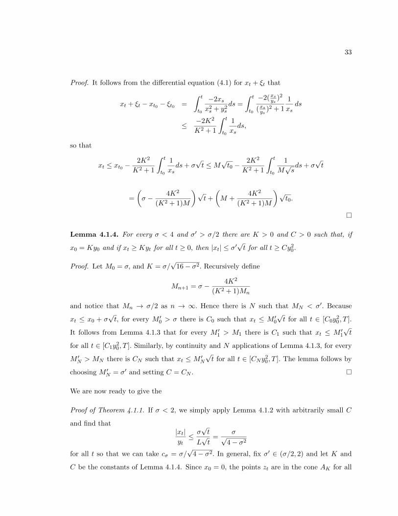
C be the constants of Lemma 4.1.4. Since x0 = 0, the points zt are in the cone AK for all

34

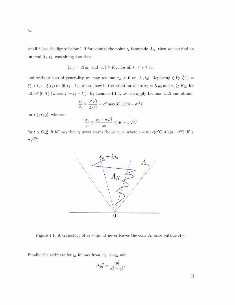
small t (see the figure below.) If for some t, the point zt is outside AK , then we can find an

interval [t1, t2] containing t so that

|xt1 | = Kyt1 and |xs| ≥ Kys for all t1 ≤ s ≤ t2,

and without loss of generality we may assume xs > 0 on [t1, t2]. Replacing ξ by ξ(·) =

ξ(·+ t1)− ξ(t1) on [0, t2− t1], we are now in the situation where x0 = Ky0 and xt ≥ Kyt for

all t ∈ [0, T ] (where T = t2 − t1). By Lemma 4.1.4, we can apply Lemma 4.1.2 and obtain

xtyt≤ σ′

√t

L√t

= σ′max(C, 1/(4− σ′2))

for t ≥ Cy20, whereas

xtyt≤ x0 + σ

√t

y0≤ K + σ

√C

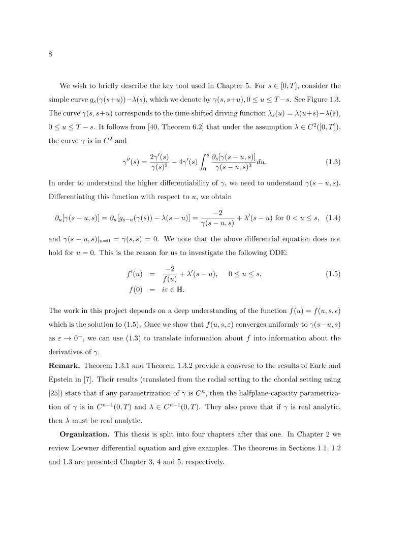
for t ≤ Cy20. It follows that zt never leaves the cone Ac where c = max(σ′C, σ′/(4−σ′2),K+

σ√C).

Figure 4.1: A trajectory of xt + iyt. It never leaves the cone Ac once outside AK .

Finally, the estimate for yt follows from |xt| ≤ cyt and

∂ty2t =

4y2t

x2t + y2

t

.

35

A simple consequence of Theorem 4.1.1 is the Holder continuity in bounded subsets of the

upper half plane of the solutions ft to the upward Loewner equation (2.3) with driving

functions satisfying σ = ||ξ|| 12< 4:

Corollary 4.1.5. If σ = ||ξ|| 12< 4, then

|f ′t(ξ0 + iy)| ≤ (4t+ y2)1−α2 yα−1

for every y > 0 and t ∈ [0, T ], where α is a constant in (0, 1] depending on σ only.

Proof. By (4.2) and (4.3), Theorem 4.1.1 implies that

|f ′t(ξ0 + iy)| ≤ exp

(∫ t

0

c2 − 1

c2 + 1

2ds

x2s + y2

s

)=

(yty

) c2−1

c2+1

≤ (4t+ y2)1−α2 yα−1,

where c = cσ and α = min1− c2−1c2+1

, 1 ∈ (0, 1].

Remark 4.1.6. The proof of Theorem 4.1.1 can easily be modified to give the following

statement: For every 0 < c1 < c2 there is σ0 such that, if z0 ∈ Ac1 and σ ≤ σ0, then

zt ∈ Ac2 for all t. Then (4.5) holds with cσ replaced by c2.

Corollary 4.1.7. There is a constant σ0 such that the following is true: If ||ξ|| 12≤ σ0, if

0 ≤ c ≤ 1 and z is in the cone Ac(ξ0), and if∫ T

0

M ξ0,s

s3/2ds <∞,

then

| arg f ′T (z)| ≤ 8c+ 4

∫ T

0

M ξ0,s

s3/2ds.

Proof. Let σ0 be the constant from Remark 4.1.6 with c1 = 1 and c2 =√

3. Then if z0 ∈ Ac

and c ≤ 1, we have zt ∈ Ac2 and yt ≥√y2

0 + t for all t by (4.5). By (4.4) and Lemma 4.0.2,

| arg f ′T (z)| ≤ 4

∫ T

0

|xs|y3s

ds

≤ 4

∫ T

0

cy0 +M ξ0,s

(y20 + s)3/2

ds

= 8cy0

(1

y0− 1√

y20 + T

)+ 4

∫ T

0

M ξ0,s

s3/2ds

≤ 8c+ 4

∫ T

0

M ξ0,s

s3/2ds.

36

4.2 The proofs of Theorems 1.2.1 and 1.2.2

Throughout this section, we maintain our notation σ = ||λ|| 12, and denote by α = ασ the

constant of Corollary 4.1.5. As explained in Chapter 2, in order to show that the Loewner

equation generates a curve it suffices to show that

v(t, ε) :=

∫ ε

0|(g−1

t )′(λt + iy)|dy

goes to zero as ε→ 0, uniformly in t ∈ [0, T ]. In our setting, this follows easily from Corollary

4.1.5:

Lemma 4.2.1. Suppose that λ : [0, T ] → R is Holder-1/2 continuous with σ < 4 and (gt)

is the solution to (1.1). Then for every ε > 0 and 0 ≤ t ≤ T ,∫ ε

0|(g−1

t )′(λt + iy)| dy ≤ (4t+ ε2)1−α2

αεα.

Proof. Fix 0 ≤ t ≤ T and ε > 0. Let ξ(s) = λ(t − s) for 0 ≤ s ≤ t. Let (fs)0≤s≤t be the

solution to (2.3) with the driving function ξ, so that g−1t = ft. Hence by Corollary 4.1.5,

|(g−1t )′(λt + iy)| = |f ′t(ξ0 + iy)| ≤ (4t+ y2)

1−α2 yα−1, (4.7)

and the lemma follows by integration.

Remark 4.2.2. By Proposition 3.9 of [9], we get a quantitative estimate for the modulus

of continuity of the trace γt := limy→0+ g−1t (λt + iy), namely γ is Holder continuous with

exponent α/2.

To complete the proof of Theorem 1.2.1, it only remains to show that γ is a simple curve

and satisfies the Ahlfors geometric characterization of quasiconformal arcs

|γt − γs| ≤M |γt − γr| (4.8)

for some constant M = Mγ and all 0 ≤ r ≤ s ≤ t ≤ T. The key idea is to use the Gehring-

Hayman inequality [28, p.72], which says that among all curves in a simply connected plane

domain with two fixed end points, the hyperbolic geodesic minimizes the euclidean length,

up to a universal multiplicative constant.

37

Lemma 4.2.3. If σ < 4, then γ is a simple curve that stays inside the cone Acσ(λ0) and

satisfies (4.8).

Proof. Again consider the upward Loewner equation (2.3) with the driving function ξ(s) =

λ(t−s) for s ∈ [0, t], for fixed t ∈ [0, T ]. It follows from Theorem 4.1.1 that for z = ξ0 + iε =

λt + iε

|xt| ≤ cσyt

and √4

1 + c2σ

t+ ε2 ≤ y2t ≤

√4t+ ε2.

Since γt = limε→0+(g−1t )(λt + iε) = limε→0+(xt + iyt + ξt), it follows that

2√t√

1 + c2σ

≤ Im γt ≤ 2√t, (4.9)

and

|Re γt − λ0| ≤ cσIm γt ≤ 2cσ√t. (4.10)

This implies that the curve γ is contained in the cone Acσ(λ0) and meets the real line

non-tangentially. It also implies that γ(0, T ] ∩ R = ∅, which easily implies that γ is simple

(Lemma 4.34 in [14]): Just notice that, if γt = γ′t for some t < t′, then gt(γ(t, T ]) intersects

the real line at λt, but that the curve gt(γ[t, T ]) has driving function λ(t) = λ(t+ t′) so that

gt(γ(t, T ]) ∩ R = ∅ by the above.

To prove (4.8), fix 0 ≤ r ≤ s ≤ t ≤ T, denote γr, γs, γt by u, v, w, and their images

under gr by u′ = λ(r), v′, w′. We may assume that the line segment (u,w) is contained in

Hr = H \ γ[0, r] (else replace u by the point u that is closest to w on (u,w) ∩ γ[0, r], and

replace r by r = γ−1(u)). By (4.9),

Im v′ ≤ 2√s− r ≤ 2

√t− r ≤

√1 + c2

σ Imw′,

so that the hyperbolic geodesic geoH(u′, v′) from u′ to v′ in H is within bounded hyperbolic

distance from geoH(u′, w′). In particular, there is a point z′ = gr(z) on geoH(u′, w′) of

bounded hyperbolic distance from v′ (where all bounds depend on cσ only). Denoting ` the

euclidean length, it follows from the Koebe distortion theorem that

|v − w| ≤ |v − z|+ |z − w| ≤ Cdist(z, ∂Hr) + `(geoHr(z, w)) ≤ C`(geoHr(u,w)),

38

since z ∈ geoHr(u, v). Since the line segment (u,w) is contained in Hr, the Gehring-Hayman

inequality implies `(geoHr(u,w)) ≤ C ′|u − w| and (4.8) follows. This finishes the proof of

Lemma 4.2.3 and of Theorem 1.2.1.

Proof of Theorem 1.2.2. Since we did not assume a priori that λ generates a curve, we first

observe that

||λ|| 12≤ 3C0. (4.11)

Indeed, since |λ(t2)−λ(t1)| ≤ 2Nλs,t2 for 0 < s ≤ t1 < t2 ≤ T , it is not hard to see that λ has

a finite Holder-1/2 norm on every interval [t1, t2] inside (0, T ]. Next, for t1 ≤ s ≤ r ≤ t ≤ t2

we have |λt − λs| ≤ Nλr,t + ||λ||1/2

√r − s. Integrating both sides of this inequality from s to

t with respect to r, dividing by (t − s)3/2 and estimating the integral involving Nλ by C0,

(4.11) easily follows by choosing s and t appropriately.

If C0 <43 , Theorem 1.2.1 applies and λ generates a curve γ. We will show that, if C0 is

small enough, then for every pair of points γ(t1), γ(t2) on γ with 0 ≤ t1 < t2 ≤ T we have

| arg(γ(t2)− γ(t1))− π

2| ≤ C <

π

2, (4.12)

where C depends on C0 and σ = ||λ|| 12

only. This implies that γ is the graph of a Lipschitz

function.

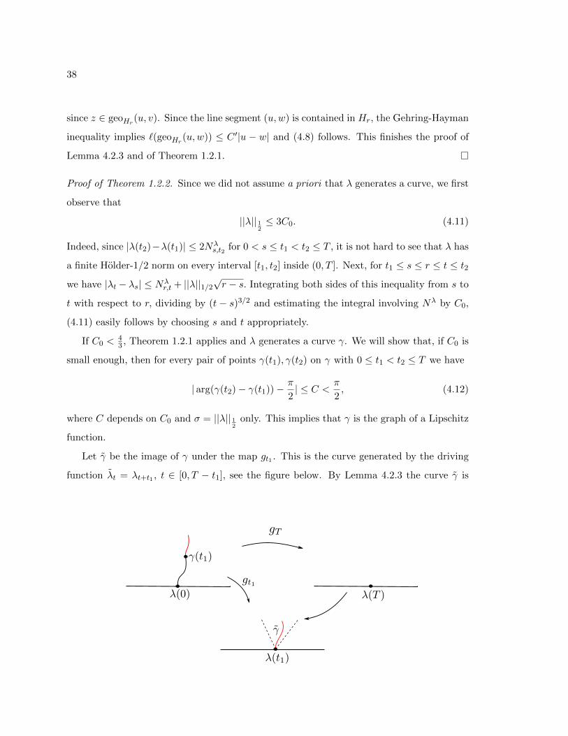
Let γ be the image of γ under the map gt1 . This is the curve generated by the driving

function λt = λt+t1 , t ∈ [0, T − t1], see the figure below. By Lemma 4.2.3 the curve γ is

39

in the cone Ac(λt1), where c = cσ is defined in Section 4.1. With w = gt1(γt2) − λt1 we

therefore have

| arg(γt2 − γt1)− π

2| = | arg(w

∫ 1

0(g−1t1

)′(λt1 + sw)ds)− π

2|

≤ arctan c+ supz∈Ac(λt1 )

| arg(g−1t1

)′(z)|.

Applying Corollary 4.1.7 to the driving function ξt = λt1−t with t ∈ [0, t1], assuming C0 is

small enough such that 3C0 < σ0 and c3C0 ≤ 1, we get

supz∈Ac(λt1 )

| arg(g−1t1

)′(z)| ≤ 8c+ 4

∫ t1

0

M ξ0,s

s3/2ds

= 8c+ 4

∫ t1

0

Nλs,t1

(t1 − s)3/2ds.

Thus

| arg(γt2 − γt1)− π

2| ≤ arctan c+ 8c+ 4C0.

If C0 → 0, then σ → 0 by (4.11) and therefore c→ 0 by Theorem 4.1.1. Thus (4.12) follows

if C0 is sufficiently small, and the theorem is proved.

40

Chapter 5

REGULARITY OF LOEWNER CURVES WHEN λ ∈ Cα WITH α > 1/2

This chapter presents joint work with Joan Lind. It is organized as follows: Section 5.1

includes initial properties of f(u, s, ε) and some lemmas regarding solutions to a particular

class of ODEs. These lemmas will be useful in analyzing f and its partial derivatives,

and this is the content of Section 5.2. In Section 5.3, we state and prove a quantitative

version of Theorem 1.3.1. Theorem 1.3.2 is proved is Section 5.4, and Theorem 1.3.4 in

Section 5.5.1. In Section 5.5.2, we prove Theorem 1.3.3 by constructing a nice curve that

well-approximates a given Loewner curve at its base. We conclude in Section 5.6 with two

examples.

5.1 Preliminaries

5.1.1 Notation

Let H = z ∈ C : Im z > 0. Let I be an interval on the real line. The space C0(I) consists

of all continuous functions on I and ||φ||∞,I = supt∈I |φ(t)| for φ ∈ C0(I).

Let α ∈ (0, 1). The function φ is in Cα if ||φ||∞,I <∞ and

||φ||Cα := sups,t∈I,s 6=t

|φ(t)− φ(s)||t− s|α

<∞.

Let n ∈ N, M > 0 and α ∈ [0, 1]. The function φ is in Cn,α(I;M) if φ′, · · · , φ(n) exist and

are continuous and the following two conditions hold:

||φ(k)||∞,I ≤M for all 0 ≤ k ≤ n,

and ||φ(n)||Cα := sups,t∈I,s 6=t

|φ(n)(t)− φ(n)(s)||t− s|α

≤M.

In particular, the nth derivative of functions in Cn,1 are Lipschitz. A function φ is in Cn if

φ ∈ Cn,0(I;M) for some M .

41

We say that φ is weakly C1(I) if φ is in Cα(I) for all 0 < α < 1, and that φ is weakly

Cn,1(I) if φ ∈ Cn and φ(n) is weakly C1. The following proposition will be needed in Section

5.5.1.

Proposition 5.1.1. If a function φ belongs to Cn,α(I;M) then there exists c = c(n,M)

such that for all t0, t+ t0 ∈ I,

|φ(t+ t0)−n∑k=0

1

k!tkφ(k)(t0)| ≤ ctn+α.

The proof follows from the integral form of the remainder of Taylor series.

In this chapter we use C for a universal constant, and c for a constant depending on M,n, T .

When constants depend on other factors, we will state this explicitly.

5.1.2 Loewner equation

It was shown that if λ ∈ C1/2[0, T ] with ||λ||C1/2 < 4 then λ generates a simple quasi-

arc γ (previous chapter and [26], [22]). Since we work with λ ∈ Cβ for β > 2, we are

guaranteed that the corresponding Loewner curve is a simple curve. Further, we can make

the assumption that ||λ||C1/2 ≤ 1 in this chapter. Indeed if λ ∈ Cβ, β > 1/2 then on small

intervals ||λ||C1/2 ≤ 1. We can apply Theorems 1.3.1 and 1.3.2 on these small intervals,

then use the concatenation property of Loewner equation to derive the regularity of γ on

[0, T ]. Henceforth, we assume ||λ||C1/2 ≤ 1.

We think of (1.5) as a variant of the backward Loewner equation (with ξ(u) = λ(s− u)

and f(u) = hu(iε) − ξ(u)), and our first goal is to understand some basic properties of its

solution f(u) = f(u, s, ε), when (u, s) ∈ D := (u, s) : 0 ≤ u ≤ s ≤ T. Further properties

of f(u, s, ε) are in Section 5.2.

Lemma 5.1.2. Let λ ∈ C1([0, T ];M), and let 0 ≤ s ≤ T and ε > 0. Then the ODE

f ′(u) =−2

f(u)+ λ′(s− u), 0 ≤ u ≤ s,

f(0) = iε ∈ H.

has a unique solution f(u) = f(u, s, ε), with 0 ≤ u ≤ s, satisfying the following properties:

(i) Im f is increasing in u.

42

(ii) For all (u, s) ∈ D = (u, s) : 0 ≤ u ≤ s ≤ T

√3u+ ε2 ≤ Im f(u, s, ε) ≤

√4u+ ε2

and |Re f(u, s, ε)| ≤√u ≤ 1√

3Im f(u, s, ε).

(iii) For every δ > 0, there is ε(δ) > 0 such that

|f(u, s, ε1)− f(u, s, ε2)| ≤ δ for all (u, s) ∈ D and ε1, ε2 ≤ ε(δ).

In particular, f(u, s, ε) converges uniformly as ε → 0+ to a limit denoted by f(u, s). This

limit is the family of curves γ(s− u, s) generated by λs, 0 ≤ s ≤ T .

(iv) Suppose λ ∈ Cn([0, T ];M), and let l+ k ≤ n and k ≤ n− 1. Then ∂lu∂ks f exists and

is continuous in (u, s) ∈ D for all ε > 0.

(v) If λ ∈ Cn([0, T ];M) and 1 ≤ k ≤ n − 1, then ∂ks f(0, s, ε) = 0 for all s ∈ [0, T ] and

ε > 0.

Proof. The equation (1.5) is of the form:

f ′(u) = G(f(u), u, s),

where G(z, u, s) = −2z + λ′(s− u) is jointly continuous in z, u, s, and Lipschitz in z variable

whenever Im z ≥ C > 0. So the solution exists on some interval containing 0. To show

that the solution to (1.5) exists on the whole interval [0, s], it suffices to show that (i)

always holds. The idea of (i)− (iii) comes from [32], which contains a study of the Loewner

equation when ||λ||C1/2 < 4. For the convenience of the reader, we will present the proof

here.

Let x = x(u), y = y(u) be real and imaginary parts of f(u). It follows from (1.5) that

(x+ λ(s− ·))′ =−2x

x2 + y2, (5.1)

y′ =2y

x2 + y2. (5.2)

In particular, y is increasing and (y2)′ ≤ 4. The former shows (i), and the latter shows that

y ≤√

4u+ ε2.

43

Now we will show that |x(u)| ≤√u, for 0 ≤ u ≤ s. Suppose 0 ≤ x(u) and let u0 = supv ∈

[0, u] : x(v) ≤ 0. So

∂v(x(v) + λ(s− v)) ≤ 0 for u0 ≤ v ≤ u,

and

x(u) + λ(s− u) ≤ x(u0) + λ(s− u0) = λ(s− u0).

Hence

x(u) ≤ λ(s− u0)− λ(s− u) ≤√|u0 − u| ≤

√u,

where the very last inequality follows since ||λ||1/2 ≤ 1. The same argument applies when

x(u) ≤ 0, proving that |x(u)| ≤√u.

Next we will show y(u) >√

3u for 0 ≤ u ≤ s. Suppose this is not the case. Then since

y(0) = ε > 0, there exists u0 ∈ (0, s] such that y(u0) =√

3u0 and y(u) ≥√

3u for u ∈ [0, u0].

It follows from (5.2) that

(y2)′ =4y2

x2 + y2≥ 12u

u+ 3u= 3 for 0 ≤ u ≤ u0.

So y(u0) ≥√

3u0 + ε2 >√

3u0. This is a contradiction. Therefore y(u) >√

3u and

(y2)′ ≥ 3. These show (ii).

To show (iii), differentiate (1.5) with respect to ε to obtain

∂u(∂εf) = ∂ε∂uf =2∂εf

f2.

Since ∂εf(0, s, ε) = i,

∂εf(u, s, ε) = i exp

∫ u

0

2

f2(v, s, ε)dv.

This implies

|∂εf(u, s, ε)| = exp

∫ u

0Re

2

f2(v, s, ε)dv

= exp

∫ u

0

2(x2(v)− y2(v))

(x2(v) + y2(v))2dv ≤ 1.

The last inequality comes from (ii). It follows that

|f(u, s, ε)− f(u, s, ε′)| ≤ |ε− ε′|, for all 0 ≤ u ≤ s ≤ T,

44

and f(u, s, ε) converges uniformly in D to a limit, denoted by f(u, s), as ε→ 0+.

Intuitively the limit f(u, s) is equal to γ(s− u, s) since f(u, s, ε) satisfies the same ODE

as γ(s−u, s) does, and limε→0+ f(0, s, ε) = γ(s−u, s)|u=0 = 0. Indeed, from (1.4) and (1.5)

we can show that

|f(u, s, ε)− γ(s− u, s)| = |f(u0, s, ε)− γ(s− u0, s)| exp

∫ u

u0

Re2 dv

f(v, s, ε)γ(s− v, s), (5.3)

with 0 < u0 ≤ u ≤ s ≤ T and ε > 0. Since γ(s − v, s) is the tip of a Loewner curve

generated by a driving function whose Holder-1/2 norm is less than 1, then by [40, Lemma

3.1], it satisfies

|Re γ(s− v, s)| ≤ Im γ(s− v, s).

This implies that

Re2

f(v, s, ε)γ(s− v, s)≤ 0.

Let u0 → 0+ and then ε→ 0+ in (5.3) we get f(u, s) = γ(s− u, s).

Statement (iv) follows from the standard ODE theory (see [6], for instance) and the fact

that G is Cn−1 in (u, s).

We show (v) by induction. For the base case,

∂sf(0, s, ε) = limδ→0

f(0, s+ δ, ε)− f(0, s, ε)

δ= lim

δ→0

ε− εδ

= 0.

Now supppose ∂ks f(0, s, ε) = 0 for all s ∈ [0, T ]. Then

∂k+1s f(0, s, ε) = lim

δ→0

∂ks f(0, s+ δ, ε)− ∂ks f(0, s, ε)

δ= 0.

Remark. For convenience, in this paper we only consider ε ∈ (0, 1]. In this case,

√3u ≤ |f(u, s, ε)| ≤

√Cu+ ε2 ≤ C

√u+ Cε ≤ c(T ) for all 0 ≤ u, s ≤ T.

Later in Lemma 5.2.2 we will show that ∂ns f exists and is continuous in (u, s).

45

5.1.3 ODE lemmas

The next lemma is one of the key tools to investigate the regularity of f(u, s, ε).

Lemma 5.1.3. Consider a complex-valued function X satisfying the initial value problem

X ′(u) = P (u)X(u) +Q(u), X(0) = 0.

Suppose |P (u)| ≤ −CReP (u) and |Q(u)| ≤M1 for 0 ≤ u ≤ u0. Then

|X(u)| ≤ (C + 1)M1u for 0 ≤ u ≤ u0.

Proof. Solving the equation, one obtains

X(u) = R(u) + e−µ(u)

∫ u

0eµ(v)P (v)R(v) dv,

where µ(u) = −∫ u

0 P (v) dv and R(u) =∫ u

0 Q(v) dv. Since |R(u)| ≤M1u,

|X(u)| ≤ M1u+M1u|e−µ(u)|∫ u

0|eµ(v)| · |P (v)| dv

≤ M1u+M1ue−Re µ(u)

∫ u

0e∫ v0 −Re P (w)dwC(−ReP (v)) dv

= M1u+ CM1ue−Re µ(u)

(e−

∫ u0 Re P (v) dv − 1

)= M1u+ CM1ue

−Re µ(u)(eRe µ(u) − 1

)≤ (C + 1)M1u.

In some cases, we will need a more general version of Lemma 5.1.3.

Lemma 5.1.4. Let Y be a solution to

Y ′(u) = P (u)Y (u)− P (u)Q(u) +R(u), Y (0) = Q(0)

with |P | ≤ −CReP and |Q(v) − Q(0)| ≤ ω(v) on [0, u0], where ω is a non-decreasing

function.

(i) If |R| ≤M2uβ−1, then

|Y (u)−Q(u)| ≤ (C + 1)ω(u) + (C + 1)M2

βuβ.

46

(ii) If Y (0) = Q(0) = 0 and |R| ≤M2, then

|Y (u)| ≤ Cω(u) + (C + 1)M2u.

(iii) More generally,

|Y (u)−Q(u)| ≤ (C + 1)ω(u) + (C + 1)

∫ u

0|R(v)| dv.

Proof. Let µ(u) =∫ u

0 −P (v) dv and S(u) =∫ u

0 R(v) dv. We have

Y (u) = e−µ(u)Y (0) + e−µ(u)

∫ u

0eµ(v)(−PQ+R) dv

= Q(0) + e−µ(u)

∫ u

0eµ(v)(−P )[Q−Q(0)] dv + e−µ(u)

∫ u

0eµ(v)Rdv

= Q(0) + e−µ(u)

∫ u

0eµ(v)(−P )[Q−Q(0)] dv + S(u)− e−µ(u)

∫ u

0eµ(v)(−P )S dv,

where the last equality follows from an integration by parts. Therefore under the first

assumption, |S(u)| ≤M2uβ/β and

|Y (u)−Q(u)| ≤ |Q(0)−Q(u)|+ e−Re µ(u)

∫ u

0eRe µ(v)C(−ReP )ω(v) dv + |S(u)|

+e−Re µ(u)

∫ u

0eRe µ(v)C(−ReP )

M2

βuβ dv

≤ ω(u) + Cω(u) +M2

βuβ + C

M2

βuβ.

Under the second assumption,

|Y (u)| ≤ e−Re µ(u)

∫ u

0eRe µ(v)C(−ReP )ω(v) dv + |S(u)|

+e−Re µ(u)

∫ u

0eRe µ(v)C(−ReP )M2u dv

≤ Cω(u) +M2u+ CM2u.

47

5.2 Properties of f(u, s, ε)

In this section, we will prove all important properties of f(u, s, ε), which are listed in the

summary after Lemma 5.2.6. Then we let ε→ 0+ to get properties of f(u, s) = γ(s− u, s).

The next two lemmas concern the s-derivatives of f .

Lemma 5.2.1. Suppose λ ∈ Cn([0, T ];M) with n ≥ 2. For every 1 ≤ k ≤ n − 1, there

exists a function Qk = Qk(u, s, ε) such that

∂u(∂ks f) =2

f2∂ks f +Qk.

with (u, s) ∈ D, and ε ∈ (0, 1]. Moreover there exists constant c = c(M,n, T ) > 0 so that

|∂ks f(u, s, ε)| ≤ cu.

Proof. We will prove the lemma by induction. Let k = 1 and n ≥ 2. Fix s ∈ [0, T ] and

ε ∈ (0, 1), and let X(u) = ∂sf(u, s, ε). Then

X ′(u) = ∂u∂sf(u, s, ε) = ∂s∂uf(u, s, ε) =2

f2(u, s, ε)∂sf(u, s, ε) + λ′′(s− u)

=2

f2(u, s, ε)X(u) + λ′′(s− u),

and X(0) = ∂sf(0, s, ε) = 0. Let Ps = Ps(u, ε) = 2f2(u,s,ε)

and Q1(u, s, ε) = λ′′(s − u).

Clearly, |Q1| ≤ M . We will show that Ps(·, ε) satisfies the property of P in Lemma 5.1.3.

Indeed, let f(u, s, ε) = x+ iy. It follows from Lemma 5.1.2(ii) that there exists a constant

C > 0 such that

|Ps(u, ε)| =2

x2 + y2≤ −C 2(x2 − y2)

(x2 + y2)2= −C RePs(u, ε).

Applying Lemma 5.1.3, we obtain

|∂sf(u, s, ε)| ≤ cu

completing the base case.

Now suppose the lemma holds for 1 ≤ k− 1 ≤ n− 2 and ∂u(∂k−1s f) = Ps∂

k−1s f +Qk−1.

Then

∂u∂ks f = ∂s(∂u∂

ks f) = Ps∂

ks f +Qk,

48

with Qk = ∂sQk−1 −4

f3(∂sf)(∂k−1

s f). One can show by induction that

Qk = λ(k+1)(s− u) +Rk

with Rk(u, s, ε) =∑

terms, where the number of terms is no more than k − 1 and each

term has the form

c

fm

m−1∏j=1

∂mjs f,

for some 3 ≤ m ≤ k + 1, and 1 ≤ mj ≤ k − 1. This term is by induction no bigger than

c

um/2um−1 = cum/2−1 ≤ c(M,k, T )

√u.

So |Qk| is bounded by a constant c = c(M,k, T ), and hence Lemma 5.1.3 implies that

|∂ks f | ≤ cu.

Remark. R1 = 0 and Rk satisfies a recursive formula:

Rk+1(u, s, ε) = ∂sRk(u, s, ε)−4

f(u, s, ε)3(∂sf(u, s, ε))(∂ks f(u, s, ε)).

We have shown that for 1 ≤ k ≤ n− 1,

|Rk| ≤ c(M,k, T )√u.

Since Rn is only related to ∂ks f for 0 ≤ k ≤ n− 1, we have the same inequality:

|Rn| ≤ c(M,n, T )√u.

Lemma 5.2.2. Suppose λ ∈ Cn([0, T ];M) then ∂ns f(u, s, ε) exists and if λ ∈ Cn,α([0, T ];M)

then

|∂ns f(u, s, ε)| ≤ cuα,

where c = c(M,n, T ).

Remark. If λ ∈ Cn([0, T ];M) then

|∂ns f(u, s, ε)| ≤ c osc(λ(n), u, [0, s]) ≤ cM.

49

Proof. It follows from the proof of the previous lemma that

∂u(∂n−1s f) = Ps∂

n−1s f +Qn−1

= Ps∂n−1s f + λ(n)(s− u) +Rn−1.

So

∂uX = PsX +Q, X|u=0 = λ(n−1)(s),

where X = ∂n−1s f + λ(n−1)(s− u) and Q = −Psλ(n−1)(s− u) +Rn−1. Since Q is C1 jointly

in (u, s), ∂sX exists and satisfies

∂u(∂sX) = Ps∂sX − Psλ(n)(s− u) +Rn.

and ∂sX|u=0 = λ(n)(s). Hence ∂ns f exists and is continuous in (u, s). Since |Rn| ≤

c(M,n, T ), apply Lemma 5.1.4 (i) with ω ≡Muα, M2 = c, and β = 1 to obtain

|∂ns f | = |∂sX − λ(n)(s− u)| ≤ (C + 1)Muα + cu ≤ cuα.

The next three lemmas concern the oscillation of ∂ks f in the variable s. In the proofs,

we omit ε from the formulas at times (for ease of reading), but we remind the reader that

the functions f, Ps, Qk, Rk do depend on three variables u, s, ε.

Lemma 5.2.3. Suppose λ ∈ C1,α([0, T ];M) with α ∈ (0, 1]. Then

|f(u, s+ δ, ε)− f(u, s, ε)| ≤ cmin(uδα, δuα),

|∂sf(u, s+ δ, ε)− ∂sf(u, s, ε)| ≤ c(1 +ε

α) min(uα, δα)

for 0 ≤ u ≤ s ≤ s+ δ ≤ T and ε > 0.

Proof. Since |∂sf(u, s, ε)| ≤ cuα (by Lemma 5.2.2),

|f(u, s+ δ, ε)− f(u, s, ε)| ≤ cδuα.

Omitting the parameter ε for convenience, we have

∂u[f(u, s+ δ)− f(u, s)] =2

f(u, s)f(u, s+ δ)[f(u, s+ δ)− f(u, s)] +λ′(s+ δ−u)−λ′(s−u),

50

and f(0, s+ δ)− f(0, s) = 0. We see that P :=2

f(u, s)f(u, s+ δ)satisfies

|P (u)| ≤ −CReP (u)

and that Q = λ′(s+ δ−u)−λ′(s−u) is bounded by Mδα. Therefore, Lemma 5.1.3 implies

|f(u, s+ δ)− f(u, s)| ≤ CMuδα.

It remains to prove the last inequality. We have

∂u[∂sf(u, s+ δ) + λ′(s+ δ − u)] = Ps+δ∂sf(u, s+ δ),

and

∂u[∂sf(u, s) + λ′(s− u)] = Ps∂sf(u, s).

So

∂u[∂sf(u, s+ δ) + λ′(s+ δ − u)− ∂sf(u, s)− λ′(s− u)]

= Ps+δ[∂sf(u, s+ δ) + λ′(s+ δ − u)− ∂sf(u, s)− λ′(s− u)]

− Ps+δ(λ′(s+ δ − u)− λ′(s− u)

)+ (Ps+δ − Ps)∂sf(u, s).

We will apply Lemma 5.1.4 with Q(u) = λ′(s + δ − u) − λ′(s − u) and R(u) = (Ps+δ −

Ps)∂sf(u, s). Note

|λ′(s+ δ − u)− λ′(s− u)− λ′(s+ δ) + λ′(s)| ≤ 2M min(uα, δα).

Further

|Ps+δ − Ps| · |∂sf(u, s)| ≤ c|f(u, s+ δ)− f(u, s)| · |f(u, s) + f(u, s+ δ)|u2

uα

≤ cuδα√Cu+ ε2

u2uα

≤ cδαuα−1/2 + cδαεuα−1,

and so ∫ u

0|R(v)| dv ≤

∫ u

0

(cδαvα−1/2 + cδαεvα−1

)dv ≤ cδαuα+1/2 + cδα

ε

αuα.

51

Therefore, by Lemma 5.1.4 (iii) with ω ≡ 2M min(uα, δα),

|∂sf(u, s+ δ)− ∂sf(u, s)| ≤ CM min(uα, δα) + cδαuα+1/2 + cδαε

αuα

≤ c(1 +ε

α) min(uα, δα).

Lemma 5.2.4. Suppose λ ∈ Cn,α([0, T ];M) with n ≥ 2 and α ∈ (0, 1]. Then

|Rk(u, s+ δ, ε)−Rk(u, s, ε)| ≤ cδ√u when 1 ≤ k ≤ n− 1,

and

|∂ks f(u, s+ δ, ε)− ∂ks f(u, s, ε)| ≤ cuδ when 1 ≤ k ≤ n− 2,

and

|∂n−1s f(u, s+ δ, ε)− ∂n−1

s f(u, s, ε)| ≤ cmin(uαδ, uδα).

Proof. From the Remark following Lemma 5.2.1, we know that R1 = 0, Rk satisfies the

recursive formula:

Rk+1 = ∂sRk −4

f3(∂sf)(∂ks f),

and |Rk| ≤ c√u for 1 ≤ k ≤ n. Therefore, for k + 1 ≤ n, Lemma 5.2.1 implies that

|∂sRk| ≤ |Rk+1|+4

|f |3|∂sf | · |∂ks f |

≤ c√u.

Thus

|Rk(u, s+ δ, ε)−Rk(u, s, ε)| ≤∫ s+δ

s|∂sRk(u, r, ε)|dr ≤ cδ

√u,

proving the first statement.

When 1 ≤ k ≤ n− 2, Lemma 5.2.1 implies that

|∂ks f(u, s+ δ, ε)− ∂ks f(u, s, ε)| ≤∫ s+δ

s|∂k+1s f(u, r, ε)|dr ≤ cuδ,

proving the second statement. From Lemma 5.2.2

|∂n−1s f(u, s+ δ, ε)− ∂n−1

s f(u, s, ε)| ≤∫ s+δ

s|∂ns f(u, r, ε)|dr ≤ cuαδ.

52

To prove the third statement, it remains to show

|∂n−1s f(u, s+ δ, ε)− ∂n−1

s f(u, s, ε)| ≤ cδαu. (5.4)

Omitting the parameter ε, we have

∂u[∂n−1s f(u, s+ δ)− ∂n−1

s f(u, s)] = Ps+δ[∂n−1s f(u, s+ δ)− ∂n−1

s f(u, s)]

+ (λ(n)(s+ δ − u)− λ(n)(s− u))

+ (Ps+δ − Ps)∂n−1s f(u, s)

+Rn−1(u, s+ δ)−Rn−1(u, s).

Since

|λ(n)(s+ δ − u)− λ(n)(s− u)| ≤Mδα,

and

|Ps+δ − Ps| · |∂n−1s f(u, s)| ≤ cδuC

u2u ≤ cδ ≤ cδα,

and

|Rn−1(u, s+ δ)−Rn−1(u, s)| ≤ cδ√u ≤ cδα,

we apply Lemma 5.1.3 with M1 = cδα to prove (5.4).

Lemma 5.2.5. Suppose λ ∈ Cn,α([0, T ];M) with n ≥ 2 and α ∈ (0, 1]. There exists

c = c(M,n, T ) so that

|Rn+1(u, s, ε)| ≤ cuα−1/2,

|Rn(u, s+ δ, ε)−Rn(u, s, ε)| ≤ cuα−1/2δ,

|∂ns f(u, s+ δ, ε)− ∂ns f(u, s, ε)| ≤ c(1 +ε

α) min(uα, δα).

Proof. Let’s note that

Rn =∑ c

fm

m−1∏j=1

∂mjs f

with 3 ≤ m ≤ n+ 1, 1 ≤ mj ≤ n− 1, and the number of terms in the sum is no more than

n− 1. Since ∂ns f exists, so does Rn+1:

Rn+1 =∑ c

fm

m−1∏j=1

∂mjs f,

53

with 3 ≤ m ≤ n+ 2 and 1 ≤ mj ≤ n. We can check that in each product, there is at most

one mj = n. Hence

|Rn+1| ≤ cnum−2uα

um/2≤ cuα+m/2−2 ≤ c(M,n, T )uα−1/2,

and

|∂sRn| ≤ |Rn+1|+4

|f |3|∂sf | · |∂ns f | ≤ cuα−1/2.

This implies that

|Rn(u, s+ δ)−Rn(u, s)| ≤ cuα−1/2δ.

It remains to prove the last statement. Now we have

∂u(∂ns f(u, s+ δ) + λ(n)(s+ δ − u)) = Ps+δ∂ns f(u, s+ δ) +Rn(u, s+ δ),

and

∂u(∂ns f(u, s) + λ(n)(s− u)) = Ps∂ns f(u, s) +Rn(u, s).

Let

Y (u) = ∂ns f(u, s+ δ) + λ(n)(s+ δ − u)− ∂ns f(u, s)− λ(n)(s− u) and

Q(u) = λ(n)(s+ δ − u)− λ(n)(s− u).

Then

∂uY = Ps+δY − Ps+δQ+ (Ps+δ − Ps)∂ns f(u, s) +Rn(u, s+ δ)−Rn(u, s).

We see that

|Q(u)−Q(0)| ≤ cmin(uα, δα),

and

|(Ps+δ − Ps)∂ns f(u, s)| ≤ cuδ√Cu+ ε2

u2uα ≤ cδuα−1/2 + cεδuα−1.

By Lemma 5.1.4 (iii) with |R(u)| ≤ cδuα−1/2 + cεδuα−1,

|∂ns f(u, s+ δ, ε)− ∂ns f(u, s, ε)| = |Y −Q| ≤ cmin(uα, δα) + cδuα+1/2 +cεδ

αuα.

54

Lemma 5.2.6. (Boundedness of mixed u and s derivatives.) Suppose λ ∈ Cn([0, T ];M).

Let s0 ∈ (0, T ) and D0 = (u, s) ∈ D : s0 ≤ u. There exists L0 = L0(M,n, T, s0) such that

for all l + k ≤ n,

|∂lu∂ks f(u, s, ε)| ≤ L0.

In other words, f ∈ Cn(D0;L0) for every ε ∈ (0, 1].

Proof. The case l = 0 and k ≤ n is proven by Lemmas 5.2.1 and 5.2.2. Consider k = 0 and

1 ≤ l ≤ n. We have

∂uf =−2

f+ λ′(s− u).

This implies that when u0 ≤ u,

|∂uf | ≤2

C√u

+M ≤ L0.

We can show by induction in l that

∂luf =2

f2∂l−1u f + (−1)l−1λ(l)(s− u) + Rl,

where Rl is the sum of a finite number (depending on l) of terms of the form

c

fm

m−1∏j=1

∂mju f

with 3 ≤ m ≤ l − 1 and 1 ≤ mj ≤ l − 2. Hence by induction |∂luf | ≤ L0 for s0 ≤ u ≤ T .

The other cases 1 ≤ k ≤ n− 1 are proved similarly.

Summary. We have proved the following properties of f(u, s, ε):

• C√u+ ε2 ≤ |f(u, s, ε)| ≤ C ′

√u+ C ′ε.

• |∂ks f(u, s, ε)| ≤ cu for 1 ≤ k ≤ n− 1.

• |∂ns f(u, s, ε)| ≤ cuα.

• |∂ks f(u, s+ δ, ε)− ∂ks f(u, s, ε)| ≤ cuδ for 1 ≤ k ≤ n− 2.

55

• |∂n−1s f(u, s+ δ, ε)− ∂n−1

s f(u, s, ε)| ≤ cmin(uδα, uαδ) if 0 ≤ n− 1.

• |∂ns f(u, s+ δ, ε)− ∂ns f(u, s, ε)| ≤ c(1 + εα) min(uα, δα) for 1 ≤ n.

• For every 0 < s0 < T , there exists L0 = L0(M,n, T, s0) such that for all l + k ≤ n,

|∂lu∂ks f(u, s, ε)| ≤ L0.

We emphasize that c depends only on M,n, T , not on α and ε. We know from Lemma

5.1.2 that f(u, s, ε) converges uniformly in D to f(u, s) as ε→ 0+. For all l+k = n, it follows

from the proof of previous lemmas that ∂lu∂ks f(u, s, ε) can be expressed in terms of lower

derivatives in u and s of f(u, s, ε). Therefore in D0 = (u, s) ∈ D : 0 < s0 ≤ u ≤ s ≤ T,

∂lu∂ks f(u, s, ε) converges uniformly. This implies that f(u, s) is in Cn(D0) and satisfies

• C√u ≤ |f(u, s)| ≤ C ′

√u.

• |∂ks f(u, s)| ≤ cu for 1 ≤ k ≤ n− 1.

• |∂ns f(u, s)| ≤ cuα.

• |∂ks f(u, s+ δ)− ∂ks f(u, s)| ≤ cuδ for 1 ≤ k ≤ n− 2.

• |∂n−1s f(u, s+ δ)− ∂n−1

s f(u, s)| ≤ cmin(uδα, uαδ) if 0 ≤ n− 1.

• |∂ns f(u, s+ δ)− ∂ns f(u, s)| ≤ cmin(uα, δα) for 1 ≤ n.

• For every 0 < s0 < T , there exists L0 = L0(M,n, T, s0) such that for all l + k ≤ n,

|∂lu∂ks f(u, s)| ≤ L0.

Corollary 5.2.7. If λ is in Cn,α[0, T ] with n ≥ 2 and α ∈ (0, 1] then γ is in Cn(0, T ].

Proof. The previous arguments imply that γ(s−u, s) ∈ Cn(D0) for every s0 ∈ (0, T ). Hence

s 7→ γ(0, s) ∈ Cn(0, T ]. Since γ(s) = γ(0, s) + λ(0), the curve γ is in Cn(0, T ].

56

5.3 Smoothness of γ

The goal of this section is to prove the following:

Theorem 5.3.1. Suppose λ ∈ Cn,α([0, T ];M) with n ≥ 2 and α ∈ (0, 1].

(i) If α < 1/2 then γ ∈ Cn,α+1/2(0, T ]. And for every 0 < s0 < T , there exists c0 =

c0(M,n, T, s0) such that γ ∈ Cn([s0, T ]; c0) and

|γ(n)(s+ δ)− γ(n)(s)| ≤ c0

1− 2αδα+1/2,

(ii) If α = 1/2 then γ is weakly in Cn,1(0, T ]. For every 0 < s0 < T , there exists

c0 = c0(M,n, T, s0) such that γ ∈ Cn([s0, T ]; c0) and

|γ(n)(s+ δ)− γ(n)(s)| ≤ c0δ(

1 + log+ s

δ

).

(iii) If α ∈ (12 , 1] then γ ∈ Cn+1,α−1/2(0, T ]. And there exists c0 = c0(M,n, T, s0) such

that

|γ(n+1)(s+ δ)− γ(n+1)(s)| ≤ c0

2α− 1δα−1/2.

Proof. Assume that λ ∈ Cn,α([0, T ];M) with n ≥ 2 and α ∈ (0, 1]. Fix s0 ∈ (0, T ) and let

D0 = (u, s) ∈ D : 0 < s0 ≤ u ≤ s ≤ T. Recall from [40] that

γ′′(s) =2γ′(s)

γ(s)2− 4γ′(s)

∫ s

0

∂s[f(u, s)]

f(u, s)3du.

We need to show

F (s) :=

∫ s

0

∂sf(u, s)

f(u, s)3du is

in Cn−2 and F (n−2) ∈ Cα+1/2 when α ∈ (0, 1/2)

in Cn−2 and F (n−2) weakly in C1 when α = 1/2

in Cn−1 and F (n−1) ∈ Cα−1/2 when α ∈ (1/2, 1]

.

Let F1(u, s) =∂sf(u, s)

f(u, s)3and R1(u, s) = 0. We define Fk and Rk recursively as follows:

Rk = ∂sRk−1 −3(∂sf)(∂k−1

s f)

f4,

Fk = ∂sFk−1 =∂ks f

f3+ Rk.

57

Let Fk(s) = Fk(s, s). Then formally

F (n−2)(s) = F(n−3)1 (s)+F

(n−4)2 (s)+ · · · Fn−2(s)+

∫ s

0

[∂n−1s f(u, s)

f3(u, s)+ Rn−1(u, s)

]du, (5.5)

and

F (n−1)(s) = F(n−2)1 (s) + F

(n−3)2 (s) + · · · Fn−1(s) +

∫ s

0

[∂ns f(u, s)

f3(u, s)+ Rn(u, s)

]du. (5.6)

We notice that

Rk =∑ c

fm

m−2∏j=1

(∂mjs f), (5.7)

where there are at most k−1 terms for the sum, 4 ≤ m ≤ k+2, and 1 ≤ mj ≤ k−1. Further,

when k ≥ 3 each product contains at most one mj = k− 1. Therefore, Rk ∈ Cn−(k−1)(D0),

Fk ∈ Cn−k(D0) and Fk ∈ Cn−k[s0, T ]. The representation of Rk in (5.7) also implies that

|Rk(u, s)| ≤ c for 1 ≤ k ≤ n, (5.8)

and |Rn+1(u, s)| ≤ c

u1/2if α ≥ 1

2. (5.9)

Hence equation (5.5) holds for all α ∈ (0, 1] and equation (5.6) holds when α ∈ (1/2, 1].

Let

Ik(s) :=

∫ s

0

∂ks f(u, s)

f(u, s)3du and IRk(s) =

∫ s

0Rk(u, s) du.

Theorem 5.3.1 will be proven once we show that

• In−1 + IRn−1 ∈ Cα+1/2[s0, T ] for α ∈ (0, 1/2),

• In−1 + IRn−1 is weakly C1[s0, T ] for α = 1/2, and

• In + IRn ∈ Cα−1/2[s0, T ] for α ∈ (1/2, 1],

along with the needed bounds on |Ik(s+ δ)− Ik(s)| and |IRk(s+ δ)− IRk(s)|. This is the

content of the next three lemmas.

58

Lemma 5.3.2. Suppose λ ∈ Cn,α([0, T ];M), with n ≥ 2 and α ∈ (0, 12 ]. Then there exists

c = c(M,n, T ) such that for all 0 < s0 ≤ s ≤ s+ δ ≤ T ,

|IRk(s+ δ)− IRk(s)| ≤ cδ for all 1 ≤ k ≤ n− 1 and

|IRn(s+ δ)− IRn(s)| ≤ cδ if α ≥ 1

2.

Proof. It follows from the definition of Rk and formula (5.8) that for 1 ≤ k ≤ n− 1,

|Rk(u, s+ δ)− Rk(u, s)| ≤∫ s+δ

s|∂vRk(u, v)| dv ≤ cδ.

Similarly if α ≥ 12 equation (5.9) implies

|Rn(u, s+ δ)− Rn(u, s)| ≤ cδ

u1/2.

Integrating completes the lemma.

Lemma 5.3.3. Suppose λ ∈ Cn,α([0, T ];M), with n ≥ 2 and α ∈ (0, 12 ]. Then In−1 ∈

Cα+1/2[s0, T ] when α ∈ (0, 1/2) and In−1 is weakly C1[s0, T ] when α = 1/2. In particular,

there exists c = c(M,n, T ) such that for all 0 < s0 ≤ s ≤ s+ δ ≤ T ,

|In−1(s+ δ)− In−1(s)| ≤

c( 11−2α + 1)δα+1/2 + c(1 + 1√

s0)δ when 0 < α < 1

2

c(1 + log+ sδ + 1√

s0)δ when α = 1

2

.

Proof. We decompose In−1(s+ δ)− In−1(s) into the sum of four integrals and bound each

integral.

In−1(s+ δ)− In−1(s) =

∫ δ∧s

0

∂n−1s f(u, s+ δ)− ∂n−1

s f(u, s)

f(u, s+ δ)3du

+

∫ s

δ∧s

∂n−1s f(u, s+ δ)− ∂n−1

s f(u, s)

f(u, s+ δ)3du

+

∫ s

0

∂n−1s f(u, s)(f(u, s)3 − f(u, s+ δ)3)

f(u, s)3f(u, s+ δ)3du

+

∫ s+δ

s

∂n−1s f(u, s+ δ)

f(u, s+ δ)3du.

The first integral:∣∣∣∣∫ δ∧s

0

∂n−1s f(u, s+ δ)− ∂n−1

s f(u, s)

f(u, s+ δ)3du

∣∣∣∣ ≤ ∫ δ∧s

0

cuδα

u3/2du

= cδα√δ ∧ s ≤ cδα+1/2.

59

The second integral, when 0 < α < 1/2:∣∣∣∣∫ s

δ∧s

∂n−1s f(u, s+ δ)− ∂n−1

s f(u, s)

f(u, s+ δ)3du

∣∣∣∣ ≤ ∫ s

δ∧s

cuαδ

u3/2du

≤ cδ

1− 2α(δα−1/2 − sα−1/2)

≤ c

1− 2αδα+1/2.

In the case α = 1/2, the second integral is bounded by∫ s

δ∧scδu−1 du = cδ log

s

s ∧ δ= cδ log+ s

δ.

The third integral:∣∣∣∣∫ s

0

∂n−1s f(u, s)(f(u, s)3 − f(u, s+ δ)3)

f(u, s)3f(u, s+ δ)3)du

∣∣∣∣ ≤ ∫ s

0

cu(uδu)

u3du

= cδs ≤ cδ.

The last integral:∣∣∣∣∫ s+δ

s

∂n−1s f(u, s+ δ)

f(u, s+ δ)3du

∣∣∣∣ ≤ ∫ s+δ

s

cu

u3/2du = c(

√s+ δ −

√s)

=cδ√

s+ δ +√s≤ c√s0δ.

Lemma 5.3.4. Suppose λ ∈ Cn,α([0, T ];M) with n ≥ 2 and α ∈ (12 , 1]. Then In ∈

Cα−1/2[s0, T ], and there exists c = c(M,T, n) such that for all 0 ≤ s ≤ s+ δ ≤ T

|In(s+ δ)− In(s)| ≤ c

2α− 1δα−1/2.

Proof. We proceed in a manner similar to the previous proof.

In(s+ δ)− In(s) =

∫ δ∧s

0

∂ns f(u, s+ δ)− ∂ns f(u, s)

f(u, s+ δ)3du

+

∫ s

δ∧s

∂ns f(u, s+ δ)− ∂ns f(u, s)

f(u, s+ δ)3du

+

∫ s

0

∂ns f(u, s)(f(u, s)3 − f(u, s+ δ)3)

f(u, s)3f(u, s+ δ)3du

+

∫ s+δ

s

∂ns f(u, s+ δ)

f(u, s+ δ)3du.

60

The first integral:∣∣∣∣∫ δ∧s

0

∂ns f(u, s+ δ)− ∂ns f(u, s)

f(u, s+ δ)3du

∣∣∣∣ ≤ ∫ δ∧s

0

cmin(uα, δα)

u3/2du

≤ c

∫ δ∧s

0uα−3/2 du ≤ c

2α− 1δα−1/2.

The second integral:∣∣∣∣∫ s

δ∧s

∂ns f(u, s+ δ)− ∂ns f(u, s)

f(u, s+ δ)3du

∣∣∣∣ ≤ ∫ s

s∧δ

cmin(uα, δα)

u3/2du

≤∫ s

s∧δ

cδα

u3/2du ≤ cδα(δ−1/2 − s−1/2) ≤ cδα−1/2.

The third integral:∣∣∣∣∫ s

0

∂ns f(u, s)(f(u, s)3 − f(u, s+ δ)3)

f(u, s)3f(u, s+ δ)3du

∣∣∣∣ ≤ ∫ s

0cuα

u2δ

u3du

=

∫ s

0cδuα−1 du =

cδ

αsα ≤ cδα−1/2.

The last integral:∣∣∣∣∫ s+δ

s

∂ns f(u, s+ δ)

f(u, s+ δ)3du

∣∣∣∣ ≤ ∫ s+δ

s

cuα

u3/2du =

c

2α− 1((s+ δ)α−1/2 − sα−1/2)

≤ c

2α− 1δα−1/2.

5.4 Real analyticity of γ

In this section we prove Theorem 1.3.2. There exists δ > 0 such that λ can be extended

(complex) analytically to E = z ∈ C : d(z, [0, T ]) ≤ δ. Notice that f(s, s) = γ(0, s) =

γ(s) − λ(0) and f(u, s, ε) converges uniformly to f(u, s) on D = (u, s) : 0 < u ≤ s, 0 <

s ≤ T. So it suffices to show that f(u, s, ε) can be extended analytically in the same

neighborhood of D (in C × C) for all ε. Recall that G(z, u, s) = −2z + λ′(s − u) is analytic

in (z, u, s), hence by the dependence of solutions of ODE on parameters (see [6, Theorem

8.1]) the function f(·, s, ε) in (1.5) exists and is analytic in a neighborhood of u = 0 for each

ε ∈ (0, 1] and s ∈ E. The main difficulty is to show this neighborhood is the same for all ε

and s.

61

The outline of this section is as follows: First we show in Lemma 5.4.1 that the equation

(1.5) still has solution when s is in the domain

E1 = t : 0 < Re t < T + δ1, |Im t| < δ1

with δ1 small enough and not depending on ε. Then in Lemma 5.4.2 we show that one can

take complex u-derivatives in (1.5), which means the solutions are extended analytically.

Finally by [6, Theorem 8.3] the solutions are analytic in (u, s) on the same domain for all ε.

Let M be an upper bound for the sup-norms of λ′ and λ′′ on E. As a first step, we will

show the following:

Lemma 5.4.1. There exists δ1 ∈ (0, δ) depending on δ,M and T such that for every s ∈ E1

and ε ∈ (0, 1], the solution to the equation

∂uf(u, s, ε) =−2

f(u, s, ε)+ λ′(s− u), u ≥ 0,

f(0, s, ε) = iε,

exists uniquely for u ∈ [0,Re s+ δ1]. Moreover,

max(√

2u,ε

2) ≤ Im f(u, s, ε) for 0 ≤ u ≤ Re s+ δ1.

Proof. The solution f(u, s, ε) exists on a neighborhood of u = 0, and it continues to exists as

long as it stays above the real line. The uniqueness of this solution comes from standard ODE

techniques. To establish the results of the lemma, we will compare f(u, s, ε) to f(u, s0, ε)

where s0 = Re s and

∂uf(u, s0, ε) =−2

f(u, s0, ε)+ λ′(s0 − u), u ≥ 0,

f(0, s0, ε) = iε.

It follows from Lemma 5.1.2 (i, ii) that

√3u+ ε2 ≤ Im f(u, s0, ε)

and |Re f(u, s0, ε)| ≤√u for 0 ≤ u ≤ s0 + δ1,

62

where δ1 < δ will be specified momentarily. By following the same argument in Lemma

5.2.3, we get a bound for the difference of f(u, s, ε) and f(u, s0, ε):

|f(u, s, ε)− f(u, s0, ε)| ≤ CMu|s− s0| ≤ CMuδ1

whenever 0 ≤ u ≤ S with

S = inf0 ≤ v ≤ u0 + δ1 : Im f(v, s, ε) <ε

3or|Re f(v, s, ε)|Im f(v, s, ε)

> C1,

where C1 is a constant in (0, 1) and close to 1. It follows that

Im f(u, s, ε) ≥ Im f(u, s0, ε)− CMuδ1 ≥√

3u+ ε2 − CMuδ1,

and

|Re f(u, s, ε)| ≤ |Re f(u, s0, ε)|+ CMuδ1 ≤√u+ CMuδ1.

By choosing δ1 small enough, Im f(u, s, ε) ≥ max(√

2u, ε/2) and

|Re f(u, s, ε)|Im f(u, s, ε)

< C1

for all 0 ≤ u ≤ S. It follows that S = u0 + δ1 and the lemma follows.

Now we will show that

Lemma 5.4.2. For every ε ∈ (0, 1], s ∈ E1 and 0 < u < Re s + δ1, there exist r =

r(u,M, δ, T ) ∈ (0, δ−δ1) and an analytic extension of f(·, s, ε) on Bu = z ∈ C : |z−u| < r

such that

∂uf(u, s, ε) =−2

f(u, s, ε)+ λ′(s− u).

Proof. We will use the Picard iteration to show that the equation

g′(u) = − 2

g(u)+ λ′(s− u), (5.10)

g(u) = f(u, s, ε)

has a solution on Bu = z ∈ C : |z − u| < r, where r will be specified later. Indeed for

|u− u| < r define g0(u) = f(u, s, ε) and

gn+1(u) = f(u, s, ε) +

∫ u

u

−2

gn(v)+ λ′(s− v) dv.

63

We will show by induction on n that gn is well-defined and analytic in Bu and

Im gn(u) ≥√u.

The base case n = 0 is clear because of Lemma 5.4.1. Suppose the claim holds for n. The

function gn+1 is well-defined and analytic in Bu since 1gn

is analytic in a simply connected

domain. Now

Im gn+1(u) ≥ Im f(u, s, ε)− |u− u|maxv∈Bu

(2

|gn(v)|+ |λ′(s− v)|

)≥√

2u− r( 2√u

+M).

The claim holds for n + 1 by choosing r small enough depending on u,M and T . We also

require that r is small enough so that 2r/u < 1. Then the sequence gn converges uniformly

in Bu since

|gn+1(u)− gn(u)| ≤ |u− u|maxv∈Bu

2|gn(v)− gn−1(v)||gn(v)gn−1(v)|

≤ 2r

u||gn − gn−1||Bu,∞.

Let g be the limit. Then this function is analytic and satisfies the differential equation

(5.10). In particular g(u) and f(u, u, ε) solve same initial value problem. Hence they are

equal when u is real. In order words, f(·, s, ε) is extended analytically on Bu.

Proof of Theorem 1.3.2. By [6, Theorem 8.3], for every ε ∈ (0, 1] the function f(u, s, ε)

is analytic in the domain (u, s) : s ∈ E1, u ∈ Bu for some u ∈ (0,Re s + δ1). It follows

that f(u, s) is also analytic in the same domain which contains (s, s) : 0 < s ≤ T. Hence

f(s, s) and γ(s) is real analytic on (0, T ].

5.5 Behavior of γ at s = 0

In this section we analyze the behavior of γ at its base, proving Theorem 1.3.4 and Theorem

1.3.3.

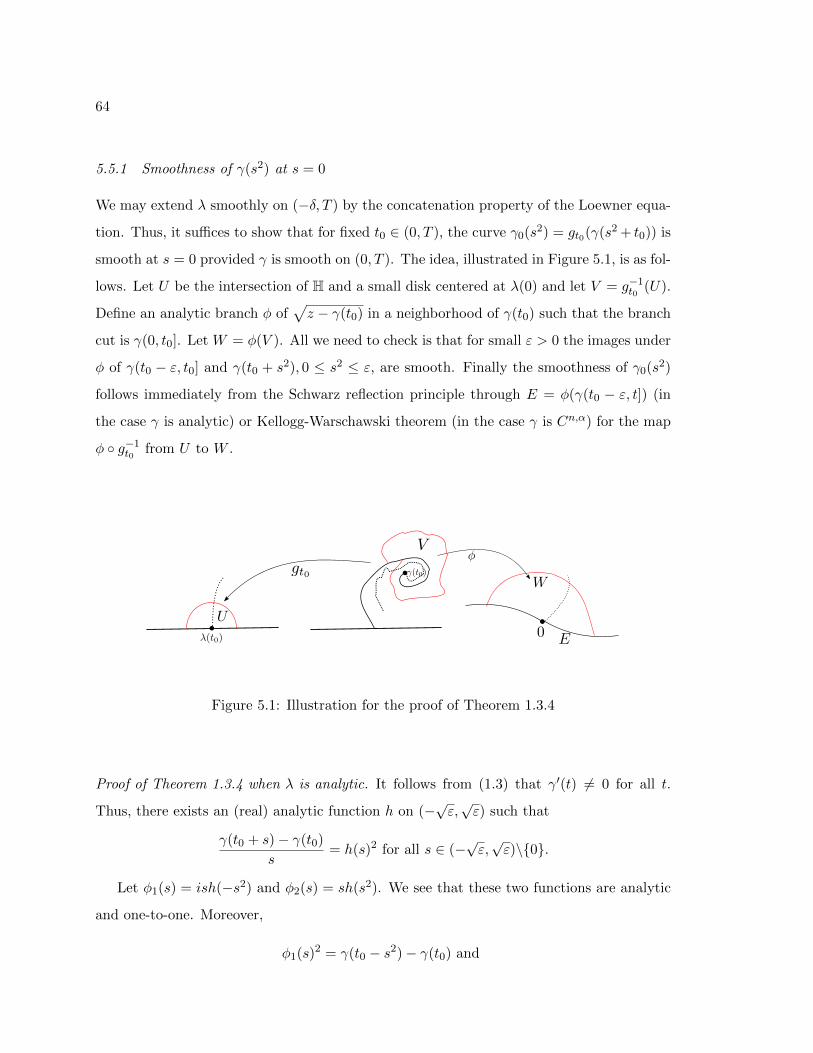
64

5.5.1 Smoothness of γ(s2) at s = 0

We may extend λ smoothly on (−δ, T ) by the concatenation property of the Loewner equa-

tion. Thus, it suffices to show that for fixed t0 ∈ (0, T ), the curve γ0(s2) = gt0(γ(s2 + t0)) is

smooth at s = 0 provided γ is smooth on (0, T ). The idea, illustrated in Figure 5.1, is as fol-

lows. Let U be the intersection of H and a small disk centered at λ(0) and let V = g−1t0

(U).

Define an analytic branch φ of√z − γ(t0) in a neighborhood of γ(t0) such that the branch

cut is γ(0, t0]. Let W = φ(V ). All we need to check is that for small ε > 0 the images under

φ of γ(t0 − ε, t0] and γ(t0 + s2), 0 ≤ s2 ≤ ε, are smooth. Finally the smoothness of γ0(s2)

follows immediately from the Schwarz reflection principle through E = φ(γ(t0 − ε, t]) (in

the case γ is analytic) or Kellogg-Warschawski theorem (in the case γ is Cn,α) for the map

φ g−1t0

from U to W .

Figure 5.1: Illustration for the proof of Theorem 1.3.4

Proof of Theorem 1.3.4 when λ is analytic. It follows from (1.3) that γ′(t) 6= 0 for all t.

Thus, there exists an (real) analytic function h on (−√ε,√ε) such that

γ(t0 + s)− γ(t0)

s= h(s)2 for all s ∈ (−

√ε,√ε)\0.

Let φ1(s) = ish(−s2) and φ2(s) = sh(s2). We see that these two functions are analytic

and one-to-one. Moreover,

φ1(s)2 = γ(t0 − s2)− γ(t0) and

65

φ2(s)2 = γ(t0 + s2)− γ(t0).

Therefore the boundary E of W , which is parametrized by φ1(s) near 0, and φ(γ(t0 + s2))

are analytic. Since the latter map is the image of γ0(s2) under φ g−1t0

, it follows from the

Schwarz reflection principle that γ0(s2) is analytic at 0.

Proof of Theorem 1.3.4 when λ is Cβ. By Theorem 1.3.4, γ ∈ Cn,α(0, T ] for appropriate

α ∈ (0, 1). It is not obvious that the function h in the previous case is Cn,α. Indeed one

can find an example of function γ ∈ Cn,α but h is not. Now let

H(s) =γ(t0 + s)− γ(t0)

sfor s ∈ (−

√ε,√ε)\0, and H(0) = γ′(t0).

We claim that H ∈ Cn−1,α(−√ε,√ε). Indeed

H(n)(s) =n!

sn+1

n∑k=0

(−1)k

k!skγ(k)(t0 + s)− (−1)nn!

sn+1γ(t0) for s 6= 0.

Apply Proposition 5.1.1 for functions γ, γ′, · · · , γ(n) to get |H(n)(s)| ≤ csα−1 which implies

the claim.

Since infs∈(−√ε,√ε) |H(s)| > 0, it follows from the claim that the function s 7→

√H(−s2)

is Cn−1,α(−√ε,√ε) for any well-defined square-root function. Let φ1(s) be a parametriza-

tion near 0 of E such that φ1(s)2 = γ(t0 − s2) − γ(t0) and φ1(s) = s√H(−s2) for

s ∈ (−√ε,√ε). Since φ′1(s) =

γ′(t0 − s2)√H(−s2)

, the function φ1 is Cn,α(−√ε,√ε). The same

argument shows that the function φ(γ(t0 + s2)) is Cn,α[0,√ε). Combined with the last two

statements, the Kellogg-Warschawski theorem [28, Theorem 3.6] implies that the function

γ0(s2) is Cn,α[0,√ε).

Remark. The proof also shows that if λ ∈ Cn,α([0, T ];M) then Γ ∈ Cn,α+1/2([0, T ]; c)

with c = c(T,M, n, α).

5.5.2 Expansion of γ at s = 0

The goal of this section is to prove Theorem 1.3.3, which illuminates why the s2 parametriza-

tion is a natural parametrization at the base of a Loewner curve γ. To accomplish this,

we create a comparison curve γ that closely approximates γ near its base and is “nice” at

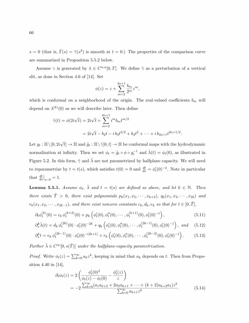
66

s = 0 (that is, Γ(s) = γ(s2) is smooth at t = 0.) The properties of the comparison curve

are summarized in Proposition 5.5.2 below.

Assume γ is generated by λ ∈ Cn,α[0, T ]. We define γ as a perturbation of a vertical

slit, as done in Section 4.6 of [14]. Set

φ(z) = z +

4n+1∑m=2

bm2m

zm,

which is conformal on a neighborhood of the origin. The real-valued coefficients bm will

depend on λ(k)(0) as we will describe later. Then define

γ(t) = φ(2i√t) = 2i

√t+

4n+1∑m=2

imbmtm/2

= 2i√t− b2t− i b3t3/2 + b4t

2 + · · ·+ i b4n+1t2n+1/2.

Let gt : H\ [0, 2i√t]→ H and gt : H\ γ[0, t]→ H be conformal maps with the hydrodynamic

normalization at infinity. Then we set φt = gt φ g−1t and λ(t) = φt(0), as illustrated in

Figure 5.2. In this form, γ and λ are not parametrized by halfplane capacity. We will need

to reparametrize by t = t(s), which satisfies t(0) = 0 and dtds = φ′t(0)−2. Note in particular

that dtds

∣∣s=0

= 1.

Lemma 5.5.1. Assume φt, λ and t = t(s) are defined as above, and let k ∈ N. Then

there exists T > 0, there exist polynomials pk(x1, x2, · · · , xk+2), qk(x1, x2, · · · , x2k) and

rk(x1, x2, · · · , x2k−1), and there exist nonzero constants ck, dk, ek so that for t ∈ [0, T ],

∂tφ(k)t (0) = ck φ

(k+2)t (0) + pk

(φ′t(0), φ′′t (0), · · · , φ(k+1)

t (0), φ′t(0)−1), (5.11)

∂ks λ(t) = dk φ(2k)t (0) · φ′t(0)−2k + qk

(φ′t(0), φ′′t (0), · · · , φ(2k−1)

t (0), φ′t(0)−1), and (5.12)

∂ks t = ek φ(2k−1)t (0) · φ′t(0)−(2k+1) + rk

(φ′t(0), φ′′t (0), · · · , φ(2k−2)

t (0), φ′t(0)−1). (5.13)

Further λ ∈ C∞[0, s(T )] under the halfplane-capacity parametrization.

Proof. Write φt(z) =∑∞

k=0 akzk, keeping in mind that ak depends on t. Then from Propo-

sition 4.40 in [14],

∂tφt(z) = 2

(φ′t(0)2

φt(z)− φt(0)− φ′t(z)

z

)= −2

∑∞k=0(a1ak+2 + 2a2ak+1 + · · ·+ (k + 2)ak+2a1)zk∑∞

k=0 ak+1zk. (5.14)

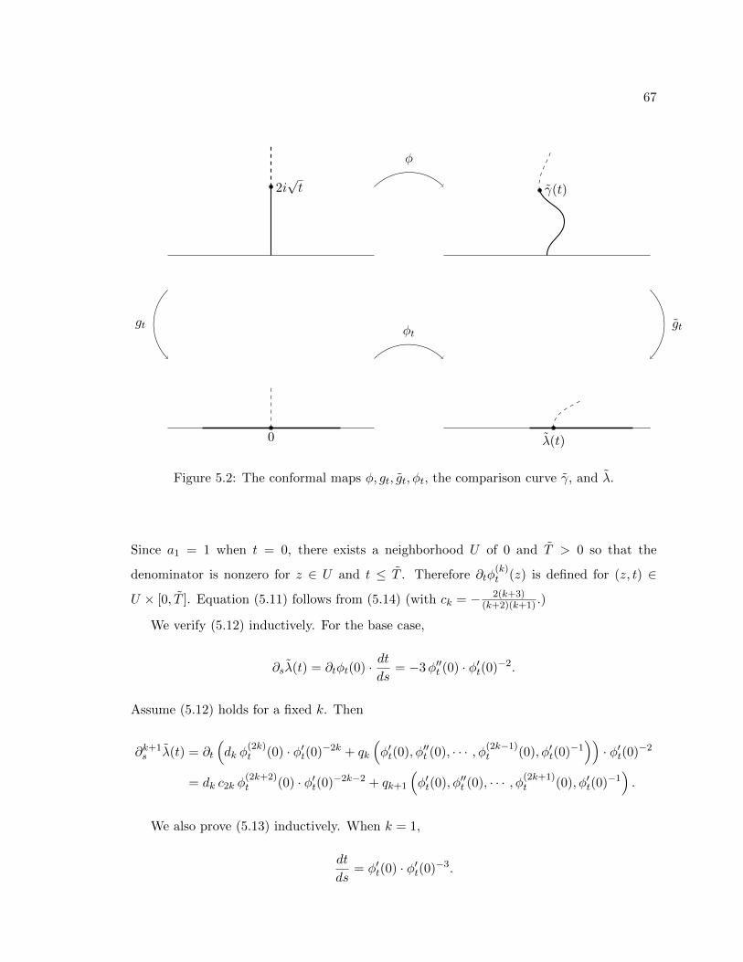
67

2i√t

φ

φtgt gt

γ(t)

0 λ(t)

Figure 5.2: The conformal maps φ, gt, gt, φt, the comparison curve γ, and λ.

Since a1 = 1 when t = 0, there exists a neighborhood U of 0 and T > 0 so that the

denominator is nonzero for z ∈ U and t ≤ T . Therefore ∂tφ(k)t (z) is defined for (z, t) ∈

U × [0, T ]. Equation (5.11) follows from (5.14) (with ck = − 2(k+3)(k+2)(k+1) .)

We verify (5.12) inductively. For the base case,

∂sλ(t) = ∂tφt(0) · dtds

= −3φ′′t (0) · φ′t(0)−2.

Assume (5.12) holds for a fixed k. Then

∂k+1s λ(t) = ∂t

(dk φ

(2k)t (0) · φ′t(0)−2k + qk

(φ′t(0), φ′′t (0), · · · , φ(2k−1)

t (0), φ′t(0)−1))· φ′t(0)−2

= dk c2k φ(2k+2)t (0) · φ′t(0)−2k−2 + qk+1

(φ′t(0), φ′′t (0), · · · , φ(2k+1)

t (0), φ′t(0)−1).

We also prove (5.13) inductively. When k = 1,

dt

ds= φ′t(0) · φ′t(0)−3.

68

If (5.13) holds for fixed k, then

∂k+1s t =

d

dt

(ek φ

(2k−1)t (0) · φ′t(0)−(2k+1) + rk

(φ′t(0), φ′′t (0), · · · , φ(2k−2)

t (0), φ′t(0)−1))· φ′t(0)−2

= ek c2k−1 φ(2k+1)t (0) · φ′t(0)−(2k+3) + rk+1

(φ′t(0), φ′′t (0), · · · , φ(2k)

t (0), φ′t(0)−1).

The last assertion follows from (5.12).

We are now ready to recursively define the coefficients of φ. The coefficient bm will

depend on λ(k)(0) for k = 1, · · · , bm2 c ∧ n. For even values of m, our choice of bm will

ensure that ∂ks λ(0) = λ(k)(0) for k ≤ n. For odd values of m, we choose bm so that the

t-parametrization of γ is close to the halfplane-capacity parametrization.

• Set b2 = −23λ′(0). Since ∂sλ(0) = −3

2b2, this implies that ∂sλ(0) = λ′(0).

• Set b3 =b228

. This implies that d2tds2

∣∣s=0

= 2b3 − b22/4 = 0.

• Assume that b2, b3, · · · , b2k−1 have been defined. Then by Lemma 5.5.1,

∂ks λ(0) = dk(2k)!

22kb2k + qk

(1,

1

2b2, · · · ,

(2k − 1)!

22k−1b2k−1, 1

).

If k ≤ n, define b2k so that ∂ks λ(0) = λ(k)(0). If k > n, we may define b2k however we

like; for instance, we choose b2k so that ∂ks λ(0) = 0.

• Assume that b2, b3, · · · , b2k have been defined. Then by Lemma 5.5.1,

dk+1t

dsk+1

∣∣∣∣s=0

= ek+1(2k + 1)!

22k+1b2k+1 + rk+1

(1,

1

2b2, · · · ,

(2k)!

22kb2k, 1

).

Define b2k+1 so that this quantity is zero.

This construction ensures that ∂ks λ(0) = λ(k)(0) for k ≤ n and that t = s + O(s2n+2).

The first fact, together with by Theorem 3.3 in [40], implies that |γ(s)− γ(t(s))| = O(sn+α)

for s near 0. The second fact implies that under the halfplane-capacity parametrization

γ(t(s)) will have the same coefficients as γ(t) for the terms with exponents at most n+ 1/2.

Together, this provides precise information about the expansion of γ(s) near s = 0. In

summary, we have proved the following, which establishes Theorem 1.3.3.

69

Proposition 5.5.2. Assume that λ ∈ Cn,α[0, T ] generates the curve γ. Then there exists

λ ∈ C∞[0, S] that generates a (half-plane capacity parametrized) curve γ ∈ C∞(0, S] with

the following properties:

• λ(k)(0) = λ(k)(0) for 1 ≤ k ≤ n.

• Γ(s) = γ(s2) is in C∞[0,√S].

• Γ(m)(0) depends on λ(k)(0) for m ≤ 2n+ 1 and k = 1, · · · , bm2 c.

• |γ(s)− γ(s)| = O(sn+α).

In particular near s = 0, the curve γ has the form

γ(s) =

2i√s+ a2s+ i a3s

3/2 + a4s2 + · · ·+ a2ns

n +O(sn+α) if α ≤ 1/2

2i√s+ a2s+ i a3s

3/2 + a4s2 + · · ·+ a2ns

n + i a2n+1sn+1/2 +O(sn+α) if α > 1/2

where the real-valued coefficients am depend on λ(k)(0) for k = 1, · · · , bm2 c.

We note the equations for the first few coefficients:

a2 =2

3λ′(0)

a3 = − 1

18λ′(0)2

a4 =4

15λ′′(0) +

1

135λ′(0)3

a5 = − 1

15λ′′(0)λ′(0) +

1

2160λ′(0)4

Coefficients a2, a3, a4 were discovered in [20] by comparison with specific example curves

(such as those generated by c√τ − t.)

Along with the tools developed in Sections 5.2 and 5.3, Proposition 5.5.2 could be used

to show that if Γ(s) = γ(s2), then Γ(k)(0) exists and equals Γ(k)(0) for k = 1, · · · , n+ 1.

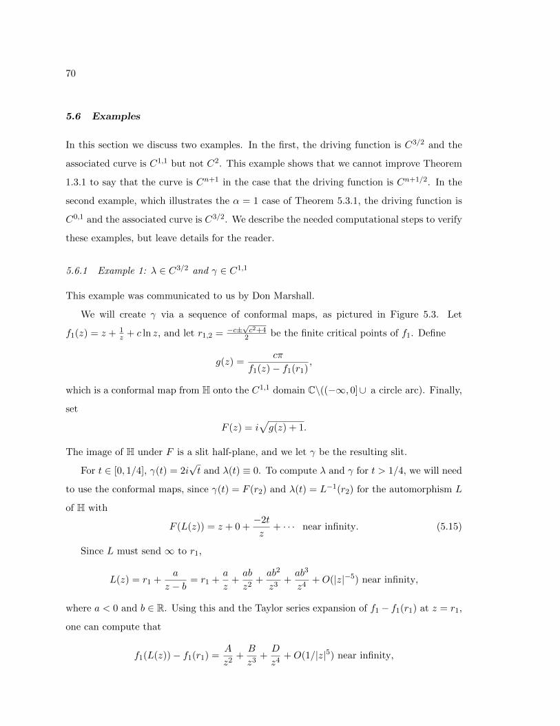
70

5.6 Examples

In this section we discuss two examples. In the first, the driving function is C3/2 and the

associated curve is C1,1 but not C2. This example shows that we cannot improve Theorem

1.3.1 to say that the curve is Cn+1 in the case that the driving function is Cn+1/2. In the

second example, which illustrates the α = 1 case of Theorem 5.3.1, the driving function is

C0,1 and the associated curve is C3/2. We describe the needed computational steps to verify

these examples, but leave details for the reader.

5.6.1 Example 1: λ ∈ C3/2 and γ ∈ C1,1

This example was communicated to us by Don Marshall.

We will create γ via a sequence of conformal maps, as pictured in Figure 5.3. Let

f1(z) = z + 1z + c ln z, and let r1,2 = −c±

√c2+4

2 be the finite critical points of f1. Define

g(z) =cπ

f1(z)− f1(r1),

which is a conformal map from H onto the C1,1 domain C\((−∞, 0]∪ a circle arc). Finally,

set

F (z) = i√g(z) + 1.

The image of H under F is a slit half-plane, and we let γ be the resulting slit.

For t ∈ [0, 1/4], γ(t) = 2i√t and λ(t) ≡ 0. To compute λ and γ for t > 1/4, we will need

to use the conformal maps, since γ(t) = F (r2) and λ(t) = L−1(r2) for the automorphism L

of H with

F (L(z)) = z + 0 +−2t

z+ · · · near infinity. (5.15)

Since L must send ∞ to r1,

L(z) = r1 +a

z − b= r1 +

a

z+ab

z2+ab2

z3+ab3

z4+O(|z|−5) near infinity,

where a < 0 and b ∈ R. Using this and the Taylor series expansion of f1 − f1(r1) at z = r1,

one can compute that

f1(L(z))− f1(r1) =A

z2+B

z3+D

z4+O(1/|z|5) near infinity,

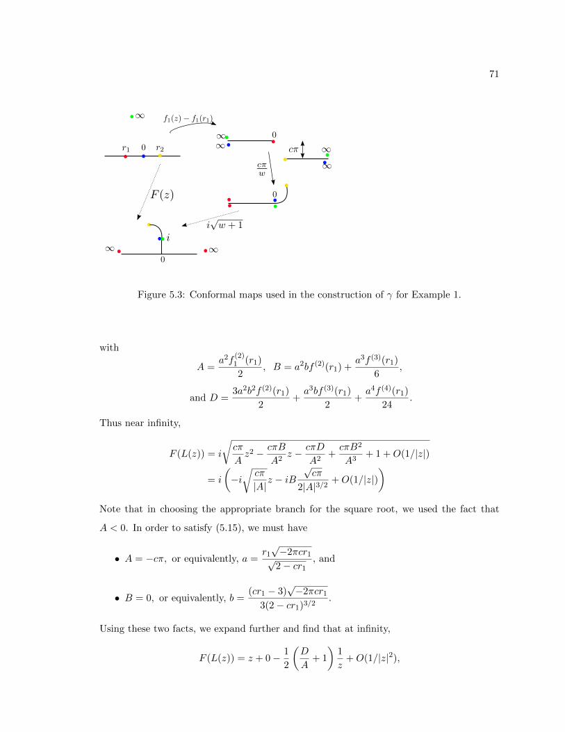
71

Figure 5.3: Conformal maps used in the construction of γ for Example 1.

with

A =a2f

(2)1 (r1)

2, B = a2bf (2)(r1) +

a3f (3)(r1)

6,

and D =3a2b2f (2)(r1)

2+a3bf (3)(r1)

2+a4f (4)(r1)

24.

Thus near infinity,

F (L(z)) = i

√cπ

Az2 − cπB

A2z − cπD

A2+cπB2

A3+ 1 +O(1/|z|)

= i

(−i√cπ

|A|z − iB

√cπ

2|A|3/2+O(1/|z|)

)Note that in choosing the appropriate branch for the square root, we used the fact that

A < 0. In order to satisfy (5.15), we must have

• A = −cπ, or equivalently, a =r1√−2πcr1√

2− cr1, and

• B = 0, or equivalently, b =(cr1 − 3)

√−2πcr1

3(2− cr1)3/2.

Using these two facts, we expand further and find that at infinity,

F (L(z)) = z + 0− 1

2

(D

A+ 1

)1

z+O(1/|z|2),

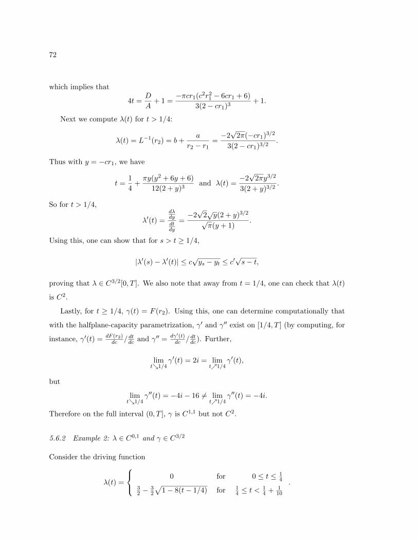
72

which implies that

4t =D

A+ 1 =

−πcr1(c2r21 − 6cr1 + 6)

3(2− cr1)3+ 1.

Next we compute λ(t) for t > 1/4:

λ(t) = L−1(r2) = b+a

r2 − r1=−2√

2π(−cr1)3/2

3(2− cr1)3/2.

Thus with y = −cr1, we have

t =1

4+πy(y2 + 6y + 6)

12(2 + y)3and λ(t) =

−2√

2πy3/2

3(2 + y)3/2.

So for t > 1/4,

λ′(t) =

dλdy

dtdy

=−2√

2√y(2 + y)3/2

√π(y + 1)

.

Using this, one can show that for s > t ≥ 1/4,

|λ′(s)− λ′(t)| ≤ c√ys − yt ≤ c′

√s− t,

proving that λ ∈ C3/2[0, T ]. We also note that away from t = 1/4, one can check that λ(t)

is C2.

Lastly, for t ≥ 1/4, γ(t) = F (r2). Using this, one can determine computationally that

with the halfplane-capacity parametrization, γ′ and γ′′ exist on [1/4, T ] (by computing, for

instance, γ′(t) = dF (r2)dc / dtdc and γ′′ = dγ′(t)

dc / dtdc). Further,

limt1/4

γ′(t) = 2i = limt1/4

γ′(t),

but

limt1/4

γ′′(t) = −4i− 16 6= limt1/4

γ′′(t) = −4i.

Therefore on the full interval (0, T ], γ is C1,1 but not C2.

5.6.2 Example 2: λ ∈ C0,1 and γ ∈ C3/2

Consider the driving function

λ(t) =

0 for 0 ≤ t ≤ 14

32 −

32

√1− 8(t− 1/4) for 1

4 ≤ t <14 + 1

10

.

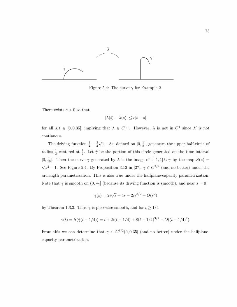
73

γ

S

γ

Figure 5.4: The curve γ for Example 2.

There exists c > 0 so that

|λ(t)− λ(s)| ≤ c|t− s|

for all s, t ∈ [0, 0.35], implying that λ ∈ C0,1. However, λ is not in C1 since λ′ is not

continuous.

The driving function 32 −

32

√1− 8s, defined on [0, 1

8 ], generates the upper half-circle of

radius 12 centered at 1

2 . Let γ be the portion of this circle generated on the time interval

[0, 110 ]. Then the curve γ generated by λ is the image of [−1, 1] ∪ γ by the map S(z) =

√z2 − 1. See Figure 5.4. By Proposition 3.12 in [27], γ ∈ C3/2 (and no better) under the

arclength parametrization. This is also true under the halfplane-capacity parametrization.

Note that γ is smooth on (0, 110 ] (because its driving function is smooth), and near s = 0

γ(s) = 2i√s+ 4s− 2is3/2 +O(s2)

by Theorem 1.3.3. Thus γ is piecewise smooth, and for t ≥ 1/4

γ(t) = S(γ(t− 1/4)) = i+ 2i(t− 1/4) + 8(t− 1/4)3/2 +O((t− 1/4)2).

From this we can determine that γ ∈ C3/2(0, 0.35] (and no better) under the halfplane-

capacity parametrization.

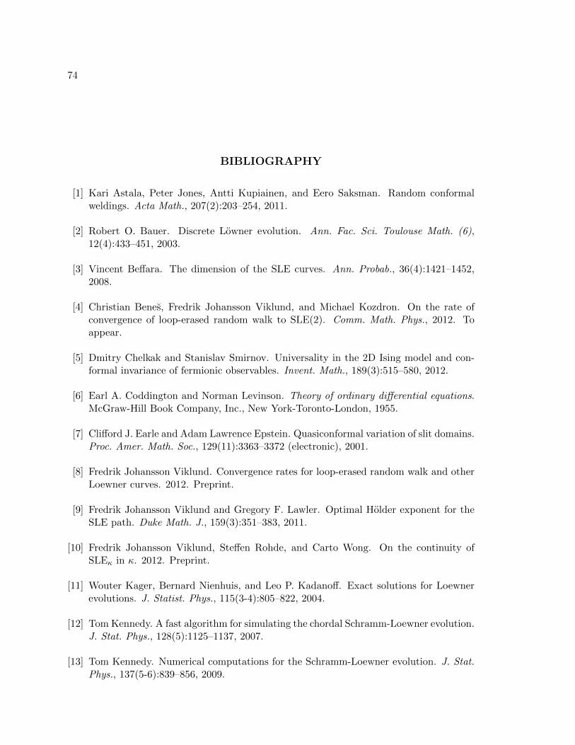
74

BIBLIOGRAPHY

[1] Kari Astala, Peter Jones, Antti Kupiainen, and Eero Saksman. Random conformalweldings. Acta Math., 207(2):203–254, 2011.

[2] Robert O. Bauer. Discrete Lowner evolution. Ann. Fac. Sci. Toulouse Math. (6),12(4):433–451, 2003.

[3] Vincent Beffara. The dimension of the SLE curves. Ann. Probab., 36(4):1421–1452,2008.

[4] Christian Benes, Fredrik Johansson Viklund, and Michael Kozdron. On the rate ofconvergence of loop-erased random walk to SLE(2). Comm. Math. Phys., 2012. Toappear.

[5] Dmitry Chelkak and Stanislav Smirnov. Universality in the 2D Ising model and con-formal invariance of fermionic observables. Invent. Math., 189(3):515–580, 2012.

[6] Earl A. Coddington and Norman Levinson. Theory of ordinary differential equations.McGraw-Hill Book Company, Inc., New York-Toronto-London, 1955.

[7] Clifford J. Earle and Adam Lawrence Epstein. Quasiconformal variation of slit domains.Proc. Amer. Math. Soc., 129(11):3363–3372 (electronic), 2001.

[8] Fredrik Johansson Viklund. Convergence rates for loop-erased random walk and otherLoewner curves. 2012. Preprint.

[9] Fredrik Johansson Viklund and Gregory F. Lawler. Optimal Holder exponent for theSLE path. Duke Math. J., 159(3):351–383, 2011.

[10] Fredrik Johansson Viklund, Steffen Rohde, and Carto Wong. On the continuity ofSLEκ in κ. 2012. Preprint.

[11] Wouter Kager, Bernard Nienhuis, and Leo P. Kadanoff. Exact solutions for Loewnerevolutions. J. Statist. Phys., 115(3-4):805–822, 2004.

[12] Tom Kennedy. A fast algorithm for simulating the chordal Schramm-Loewner evolution.J. Stat. Phys., 128(5):1125–1137, 2007.

[13] Tom Kennedy. Numerical computations for the Schramm-Loewner evolution. J. Stat.Phys., 137(5-6):839–856, 2009.

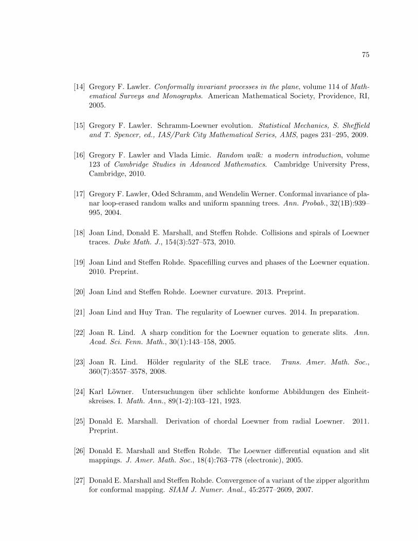
75

[14] Gregory F. Lawler. Conformally invariant processes in the plane, volume 114 of Math-ematical Surveys and Monographs. American Mathematical Society, Providence, RI,2005.

[15] Gregory F. Lawler. Schramm-Loewner evolution. Statistical Mechanics, S. Sheffieldand T. Spencer, ed., IAS/Park City Mathematical Series, AMS, pages 231–295, 2009.

[16] Gregory F. Lawler and Vlada Limic. Random walk: a modern introduction, volume123 of Cambridge Studies in Advanced Mathematics. Cambridge University Press,Cambridge, 2010.

[17] Gregory F. Lawler, Oded Schramm, and Wendelin Werner. Conformal invariance of pla-nar loop-erased random walks and uniform spanning trees. Ann. Probab., 32(1B):939–995, 2004.

[18] Joan Lind, Donald E. Marshall, and Steffen Rohde. Collisions and spirals of Loewnertraces. Duke Math. J., 154(3):527–573, 2010.

[19] Joan Lind and Steffen Rohde. Spacefilling curves and phases of the Loewner equation.2010. Preprint.

[20] Joan Lind and Steffen Rohde. Loewner curvature. 2013. Preprint.

[21] Joan Lind and Huy Tran. The regularity of Loewner curves. 2014. In preparation.

[22] Joan R. Lind. A sharp condition for the Loewner equation to generate slits. Ann.Acad. Sci. Fenn. Math., 30(1):143–158, 2005.

[23] Joan R. Lind. Holder regularity of the SLE trace. Trans. Amer. Math. Soc.,360(7):3557–3578, 2008.

[24] Karl Lowner. Untersuchungen uber schlichte konforme Abbildungen des Einheit-skreises. I. Math. Ann., 89(1-2):103–121, 1923.

[25] Donald E. Marshall. Derivation of chordal Loewner from radial Loewner. 2011.Preprint.

[26] Donald E. Marshall and Steffen Rohde. The Loewner differential equation and slitmappings. J. Amer. Math. Soc., 18(4):763–778 (electronic), 2005.

[27] Donald E. Marshall and Steffen Rohde. Convergence of a variant of the zipper algorithmfor conformal mapping. SIAM J. Numer. Anal., 45:2577–2609, 2007.

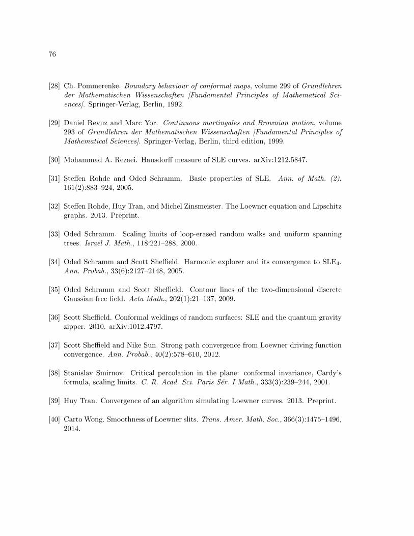
76

[28] Ch. Pommerenke. Boundary behaviour of conformal maps, volume 299 of Grundlehrender Mathematischen Wissenschaften [Fundamental Principles of Mathematical Sci-ences]. Springer-Verlag, Berlin, 1992.

[29] Daniel Revuz and Marc Yor. Continuous martingales and Brownian motion, volume293 of Grundlehren der Mathematischen Wissenschaften [Fundamental Principles ofMathematical Sciences]. Springer-Verlag, Berlin, third edition, 1999.

[30] Mohammad A. Rezaei. Hausdorff measure of SLE curves. arXiv:1212.5847.

[31] Steffen Rohde and Oded Schramm. Basic properties of SLE. Ann. of Math. (2),161(2):883–924, 2005.

[32] Steffen Rohde, Huy Tran, and Michel Zinsmeister. The Loewner equation and Lipschitzgraphs. 2013. Preprint.

[33] Oded Schramm. Scaling limits of loop-erased random walks and uniform spanningtrees. Israel J. Math., 118:221–288, 2000.

[34] Oded Schramm and Scott Sheffield. Harmonic explorer and its convergence to SLE4.Ann. Probab., 33(6):2127–2148, 2005.

[35] Oded Schramm and Scott Sheffield. Contour lines of the two-dimensional discreteGaussian free field. Acta Math., 202(1):21–137, 2009.

[36] Scott Sheffield. Conformal weldings of random surfaces: SLE and the quantum gravityzipper. 2010. arXiv:1012.4797.

[37] Scott Sheffield and Nike Sun. Strong path convergence from Loewner driving functionconvergence. Ann. Probab., 40(2):578–610, 2012.

[38] Stanislav Smirnov. Critical percolation in the plane: conformal invariance, Cardy’sformula, scaling limits. C. R. Acad. Sci. Paris Ser. I Math., 333(3):239–244, 2001.

[39] Huy Tran. Convergence of an algorithm simulating Loewner curves. 2013. Preprint.

[40] Carto Wong. Smoothness of Loewner slits. Trans. Amer. Math. Soc., 366(3):1475–1496,2014.