c© 2016 Matthew L.S. Zappulla

GRADE EFFECTS ON THERMAL-MECHANICAL BEHAVIOR DURINGTHE INITIAL SOLIDIFICATION OF STEEL

BY

MATTHEW L.S. ZAPPULLA

THESIS

Submitted in partial fulfillment of the requirementsfor the degree of Master of Science in Mechanical Engineering

in the Graduate College of theUniversity of Illinois at Urbana-Champaign, 2016

Urbana, Illinois

Adviser:

Professor Brian G. Thomas

Abstract

This work takes initial steps towards the ultimate goal of fundamental understand-

ing of how cracks and depressions form during continuous casting of steel, and

demonstrates a tool towards troubleshooting and preventing them. Mathematical

models are developed and applied to examine thermal and mechanical behavior

in the mold region of the continuous casting process. First, the models are used

to study the effect of changes in steel grade early in the process for uniform so-

lidification. Next, a thermal resistor model was developed of the interfacial gap,

and finally, these two models are combined for a preliminary coupled analysis of

a depression.

The effect of different steel grade on the relevant behavior is captured accord-

ing to the phase fractions and the properties of each phase. The model is validated

using analytical solutions, and applied to explore the behavior of four different

steel grades: Ultra-Low Carbon (0.003 %C), Low Carbon (0.04 %C), Peritectic

(0.13 %C), and High Carbon (0.47 %C), simulating 30 s dwell times. Mesh re-

finement for capturing solidification details was examined and element sizes of

0.1 mm or smaller may be required to properly study solidification phenomena.

All steel grades were found to follow the same general solidification behavior of

compression at the surface increasing with time, and tension towards the solidifica-

tion front. The initial solidification rate increases with carbon content. Thermal

strain dominates the mechanical behavior. More stress and inelastic strain are

generated in the high carbon steels, because they are mainly composed of high-

strength austenite. Stress in the δ-ferrite phase is always very small, owing to the

low strength of this phase. This simple model can help in the calculation of taper

ii

profiles for different steel grades and maintain the desired contact with the mold.

While fixed linear taper practices are common in industry, this work demonstrates

that the desired profile of the shell is actually parabolic.

A thermal resistor model was developed to examine heat transfer phenomena

within the interfacial gap during continuous casting. Results show that increasing

slag layer thickness decreases heat flux across the gap. In addition, decreasing

solidification temperature of the mold flux, for a fixed gap size, leads to more

high-conductivity liquid present in the gap, so the heat flux rises. Finally, this

work demonstrates an example of combining the realistic thermal-resistor model

of the gap together with the thermal-mechanical model to show the different local

behavior that can occur at a depression. Differences in flux layer thickness at

the depression cause a drop in heat flux, higher surface temperatures, and a drop

in shell thickness, which can result in necking phenomena in the solid shell as

the stress from the shrinkage of the surrounding material concentrates in thinned

shell regions.

This work is the first step in demonstrating a transient 3-D model of thermal-

mechanical behavior to examine the formation of cracks and depressions - where

the correct behavior can be verified in a simplified case where an analytical solu-

tion exists, while allowing for extensions to higher dimensional modeling work in

the future.

iii

For R.L.Z. & L.B.P.Z.

You taught me to always have a plan.

iv

Acknowledgments

I would like to thank my advisor Professor Brian G. Thomas for his unflinching

support and guidance through the past 4 years of work, thank you for always

asking the right questions at the right times.

All the students of the CCC: Kenny Swartz, Eric Badger, Aravind Murali, Bren-

dan Joyce, Gavin Hamilton, Pete Srisuk, Ramnik Singh, Seong-Mook Cho, Prathiba

Divuuri, Adnan Akhtar, Hyung-Jin Lee, Hyunjin Yang, Kun Xu, Kai Jin, Nathan

Seymour, Yonghui Li, Xialou Yan, A.S.M. Jonayat

Particular mention to Dr. Lance C. Hibbeler, Dr. Bryan Petrus, Dr. Rui Liu,

and Dr. Joydeep Sengupta for many shared pints of advice; as well as Dr. Seid

Koric for his helpful support with HPC and when ABAQUS just doesn’t want to

work.

I also gratefully acknowledge the financial support by the member companies

of the Continuous Casting Consortium at the University of Illinois at Urbana-

Champaign, whos current members include: ANSYS-Fluent, Baosteel, Nucor,

Magnesita Refractories, Arcelor-Mittal, SSAB, Postech/Posco, AK Steel, ABB,

Nippon Steel and Sumitomo Metals Corp., JFE Steel, Severstal, and Tata Steel.

This work was also supported by the National Science Foundation (Grant Num-

ber: CMMI-1300907), as well as part of the Blue Waters sustained-petascale com-

puting project, which is supported by the National Science Foundation (awards

OCI-0725070 and ACI-1238993) and the state of Illinois. Blue Waters is a joint

effort of the University of Illinois at Urbana-Champaign and its National Center

for Supercomputing Applications.

v

This work would also not have been possible without the support of all my

friends, you truly helped me keep my sanity.

vi

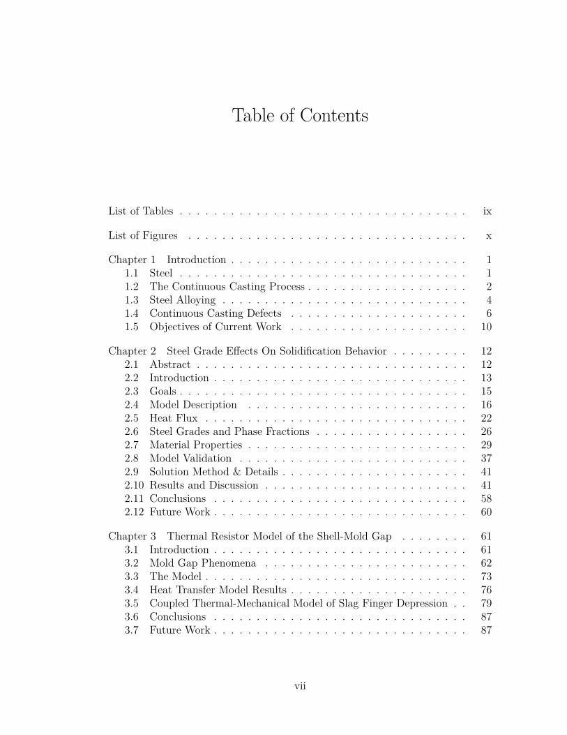
Table of Contents

List of Tables . . . . . . . . . . . . . . . . . . . . . . . . . . . . . . . . . . ix

List of Figures . . . . . . . . . . . . . . . . . . . . . . . . . . . . . . . . . x

Chapter 1 Introduction . . . . . . . . . . . . . . . . . . . . . . . . . . . . 11.1 Steel . . . . . . . . . . . . . . . . . . . . . . . . . . . . . . . . . . 11.2 The Continuous Casting Process . . . . . . . . . . . . . . . . . . . 21.3 Steel Alloying . . . . . . . . . . . . . . . . . . . . . . . . . . . . . 41.4 Continuous Casting Defects . . . . . . . . . . . . . . . . . . . . . 61.5 Objectives of Current Work . . . . . . . . . . . . . . . . . . . . . 10

Chapter 2 Steel Grade Effects On Solidification Behavior . . . . . . . . . 122.1 Abstract . . . . . . . . . . . . . . . . . . . . . . . . . . . . . . . . 122.2 Introduction . . . . . . . . . . . . . . . . . . . . . . . . . . . . . . 132.3 Goals . . . . . . . . . . . . . . . . . . . . . . . . . . . . . . . . . . 152.4 Model Description . . . . . . . . . . . . . . . . . . . . . . . . . . 162.5 Heat Flux . . . . . . . . . . . . . . . . . . . . . . . . . . . . . . . 222.6 Steel Grades and Phase Fractions . . . . . . . . . . . . . . . . . . 262.7 Material Properties . . . . . . . . . . . . . . . . . . . . . . . . . . 292.8 Model Validation . . . . . . . . . . . . . . . . . . . . . . . . . . . 372.9 Solution Method & Details . . . . . . . . . . . . . . . . . . . . . . 412.10 Results and Discussion . . . . . . . . . . . . . . . . . . . . . . . . 412.11 Conclusions . . . . . . . . . . . . . . . . . . . . . . . . . . . . . . 582.12 Future Work . . . . . . . . . . . . . . . . . . . . . . . . . . . . . . 60

Chapter 3 Thermal Resistor Model of the Shell-Mold Gap . . . . . . . . 613.1 Introduction . . . . . . . . . . . . . . . . . . . . . . . . . . . . . . 613.2 Mold Gap Phenomena . . . . . . . . . . . . . . . . . . . . . . . . 623.3 The Model . . . . . . . . . . . . . . . . . . . . . . . . . . . . . . . 733.4 Heat Transfer Model Results . . . . . . . . . . . . . . . . . . . . . 763.5 Coupled Thermal-Mechanical Model of Slag Finger Depression . . 793.6 Conclusions . . . . . . . . . . . . . . . . . . . . . . . . . . . . . . 873.7 Future Work . . . . . . . . . . . . . . . . . . . . . . . . . . . . . . 87

vii

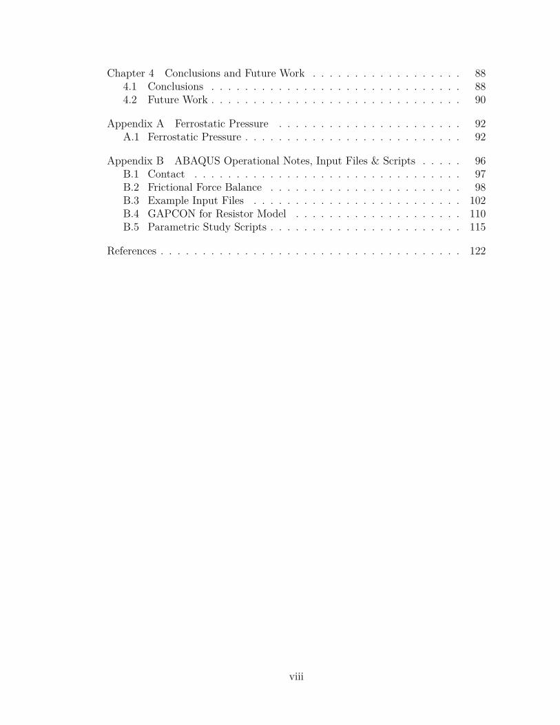
Chapter 4 Conclusions and Future Work . . . . . . . . . . . . . . . . . . 884.1 Conclusions . . . . . . . . . . . . . . . . . . . . . . . . . . . . . . 884.2 Future Work . . . . . . . . . . . . . . . . . . . . . . . . . . . . . . 90

Appendix A Ferrostatic Pressure . . . . . . . . . . . . . . . . . . . . . . 92A.1 Ferrostatic Pressure . . . . . . . . . . . . . . . . . . . . . . . . . . 92

Appendix B ABAQUS Operational Notes, Input Files & Scripts . . . . . 96B.1 Contact . . . . . . . . . . . . . . . . . . . . . . . . . . . . . . . . 97B.2 Frictional Force Balance . . . . . . . . . . . . . . . . . . . . . . . 98B.3 Example Input Files . . . . . . . . . . . . . . . . . . . . . . . . . 102B.4 GAPCON for Resistor Model . . . . . . . . . . . . . . . . . . . . 110B.5 Parametric Study Scripts . . . . . . . . . . . . . . . . . . . . . . . 115

References . . . . . . . . . . . . . . . . . . . . . . . . . . . . . . . . . . . . 122

viii

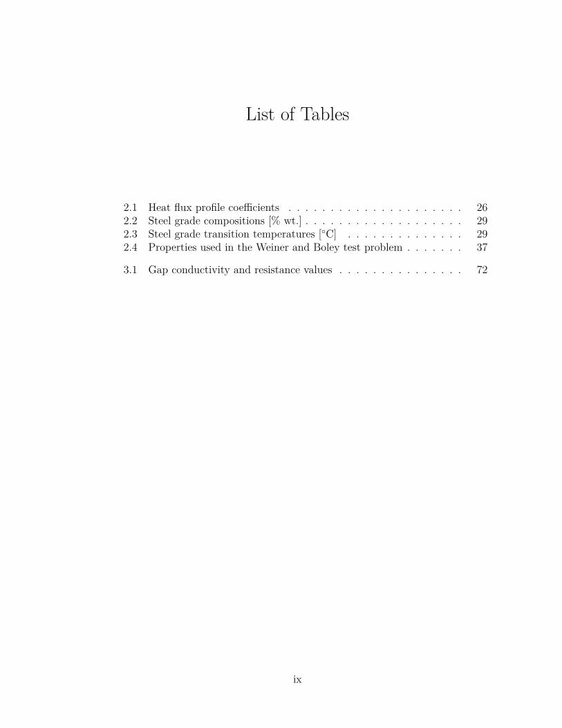
List of Tables

2.1 Heat flux profile coefficients . . . . . . . . . . . . . . . . . . . . . 262.2 Steel grade compositions [% wt.] . . . . . . . . . . . . . . . . . . . 292.3 Steel grade transition temperatures [◦C] . . . . . . . . . . . . . . 292.4 Properties used in the Weiner and Boley test problem . . . . . . . 37

3.1 Gap conductivity and resistance values . . . . . . . . . . . . . . . 72

ix

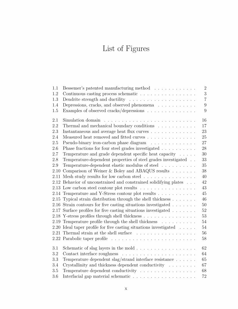
List of Figures

1.1 Bessemer’s patented manufacturing method . . . . . . . . . . . . 21.2 Continuous casting process schematic . . . . . . . . . . . . . . . . 31.3 Dendrite strength and ductility . . . . . . . . . . . . . . . . . . . 71.4 Depressions, cracks, and observed phenomena . . . . . . . . . . . 91.5 Examples of observed cracks/depressions . . . . . . . . . . . . . . 9

2.1 Simulation domain . . . . . . . . . . . . . . . . . . . . . . . . . . 162.2 Thermal and mechanical boundary conditions . . . . . . . . . . . 172.3 Instantaneous and average heat flux curves . . . . . . . . . . . . . 232.4 Measured heat removed and fitted curves . . . . . . . . . . . . . . 252.5 Pseudo-binary iron-carbon phase diagram . . . . . . . . . . . . . 272.6 Phase fractions for four steel grades investigated . . . . . . . . . . 282.7 Temperature and grade dependent specific heat capacity . . . . . 302.8 Temperature-dependent properties of steel grades investigated . . 332.9 Temperature-dependent elastic modulus of steel . . . . . . . . . . 352.10 Comparison of Weiner & Boley and ABAQUS results . . . . . . . 382.11 Mesh study results for low carbon steel . . . . . . . . . . . . . . . 402.12 Behavior of unconstrained and constrained solidifying plates . . . 422.13 Low carbon steel contour plot results . . . . . . . . . . . . . . . . 432.14 Temperature and Y-Stress contour plot results . . . . . . . . . . . 452.15 Typical strain distribution through the shell thickness . . . . . . . 462.16 Strain contours for five casting situations investigated . . . . . . . 502.17 Surface profiles for five casting situations investigated . . . . . . . 522.18 Y-stress profiles through shell thickness . . . . . . . . . . . . . . . 532.19 Temperature profile through the shell thickness . . . . . . . . . . 542.20 Ideal taper profile for five casting situations investigated . . . . . 542.21 Thermal strain at the shell surface . . . . . . . . . . . . . . . . . 562.22 Parabolic taper profile . . . . . . . . . . . . . . . . . . . . . . . . 58

3.1 Schematic of slag layers in the mold . . . . . . . . . . . . . . . . . 623.2 Contact interface roughness . . . . . . . . . . . . . . . . . . . . . 643.3 Temperature dependent slag/strand interface resistance . . . . . . 653.4 Crystallinity and thickness dependent conductivity . . . . . . . . 673.5 Temperature dependent conductivity . . . . . . . . . . . . . . . . 683.6 Interfacial gap material schematic . . . . . . . . . . . . . . . . . . 72

x

3.7 Interfacial gap resistor schematic . . . . . . . . . . . . . . . . . . 733.8 Calculation flowchart for resistor model . . . . . . . . . . . . . . . 753.9 Projected and actual heat flux . . . . . . . . . . . . . . . . . . . . 763.10 Flux layer thickness variation . . . . . . . . . . . . . . . . . . . . 773.11 Effect of solidification temperature variation . . . . . . . . . . . . 783.12 Time varying flux thickness . . . . . . . . . . . . . . . . . . . . . 783.13 Slag finger domain . . . . . . . . . . . . . . . . . . . . . . . . . . 803.14 Slag finger mesh . . . . . . . . . . . . . . . . . . . . . . . . . . . . 803.15 Slag finger thermal boundary conditions . . . . . . . . . . . . . . 813.16 Slag finger model implementation . . . . . . . . . . . . . . . . . . 813.17 Slag finger mechanical boundary conditions . . . . . . . . . . . . . 823.18 Slag finger model results . . . . . . . . . . . . . . . . . . . . . . . 833.19 Slag finger model deformed shape . . . . . . . . . . . . . . . . . . 843.20 Y-heat flux contour plot showing distorted elements . . . . . . . . 843.21 Slag finger temperature results . . . . . . . . . . . . . . . . . . . . 853.22 Slag finger liquid fraction contour . . . . . . . . . . . . . . . . . . 863.23 Slag finger thermal boundary conditions . . . . . . . . . . . . . . 86

A.1 Ferrostatic pressure applied pulling on domain . . . . . . . . . . . 93A.2 Ferrostatic pressure applied pushing on domain . . . . . . . . . . 94A.3 Results of varied ferrostatic pressure application . . . . . . . . . . 95

B.1 Internal force balance at 10 s . . . . . . . . . . . . . . . . . . . . . 99B.2 External force balance at 10 s . . . . . . . . . . . . . . . . . . . . 100

xi

Chapter 1

Introduction

1.1 Steel

Steel by definition is a metal alloy that is composed primarily of Iron and Carbon;

yet for it’s seeming simplicity, steel is one of the most versatile and fundamental

building blocks of the modern world.

Steelmaking has evolved over the course of hundreds of years from the black-

smiths of the middle ages [1] to the Bessemer process [2]. The process patented

by Bessemer in the mid 1800’s, shown in Figure 1.1, is quite similar to the method

employed in modern strip casting. However, at the time of the patent it proved

very difficult to control and the quality of the final products was far inferior to

other methods [3] which slowed it’s adoption.

The introduction of mold oscillation in the 1930’s by Siegfried Junghans brought

about the start of a functionally continuous process. Further developments in the

1950’s and 60’s saw the development of modern continuous casting [4] including

the successful operation of the worlds first production scale continuous casting ma-

chines [3]. In the beginning only vertical casters were constructed, this presented

issues due to the long time period required for complete solidification. Intro-

duction of the arc-type machine alleviated this difficulty, and continuous casting

quickly began to spread, and by the 1990’s was the production method for the

majority of the world’s total crude steel.

Steel offers one of the most efficient cost-to-weight ratios of any manufacturing

material and it’s strength is unparalleled. It is found everywhere from construction

equipment to construction material, infrastructure to transportation, and even

1

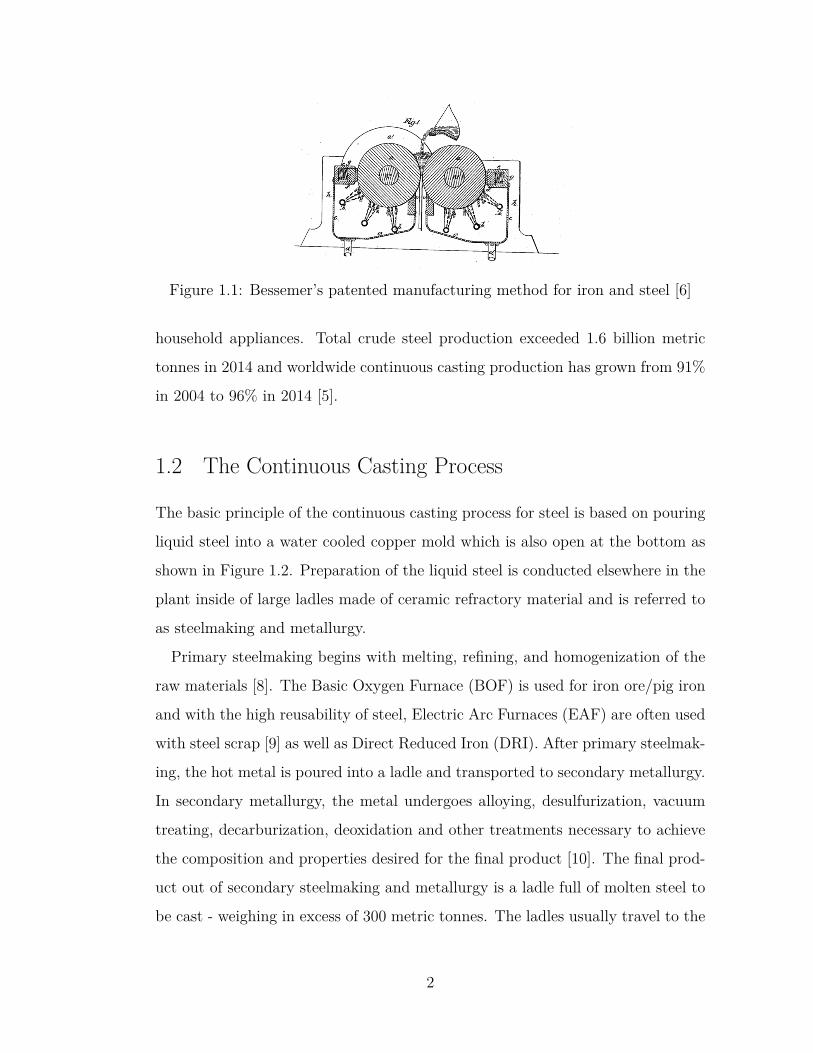
Figure 1.1: Bessemer’s patented manufacturing method for iron and steel [6]

household appliances. Total crude steel production exceeded 1.6 billion metric

tonnes in 2014 and worldwide continuous casting production has grown from 91%

in 2004 to 96% in 2014 [5].

1.2 The Continuous Casting Process

The basic principle of the continuous casting process for steel is based on pouring

liquid steel into a water cooled copper mold which is also open at the bottom as

shown in Figure 1.2. Preparation of the liquid steel is conducted elsewhere in the

plant inside of large ladles made of ceramic refractory material and is referred to

as steelmaking and metallurgy.

Primary steelmaking begins with melting, refining, and homogenization of the

raw materials [8]. The Basic Oxygen Furnace (BOF) is used for iron ore/pig iron

and with the high reusability of steel, Electric Arc Furnaces (EAF) are often used

with steel scrap [9] as well as Direct Reduced Iron (DRI). After primary steelmak-

ing, the hot metal is poured into a ladle and transported to secondary metallurgy.

In secondary metallurgy, the metal undergoes alloying, desulfurization, vacuum

treating, decarburization, deoxidation and other treatments necessary to achieve

the composition and properties desired for the final product [10]. The final prod-

uct out of secondary steelmaking and metallurgy is a ladle full of molten steel to

be cast - weighing in excess of 300 metric tonnes. The ladles usually travel to the

2

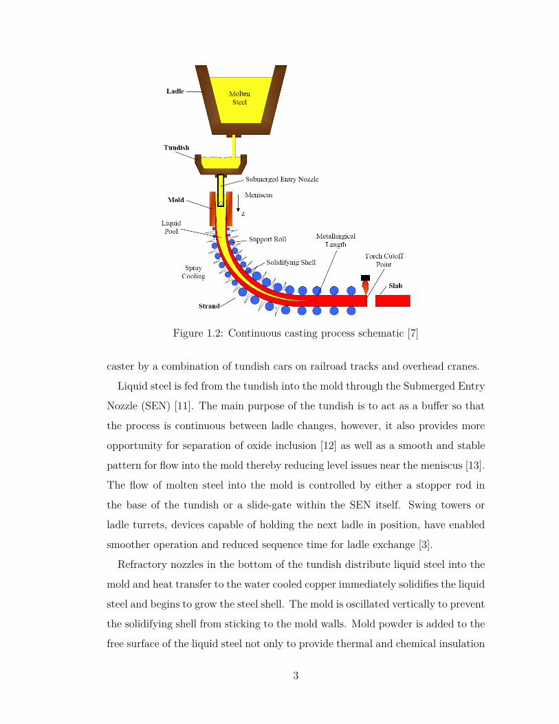
Figure 1.2: Continuous casting process schematic [7]

caster by a combination of tundish cars on railroad tracks and overhead cranes.

Liquid steel is fed from the tundish into the mold through the Submerged Entry

Nozzle (SEN) [11]. The main purpose of the tundish is to act as a buffer so that

the process is continuous between ladle changes, however, it also provides more

opportunity for separation of oxide inclusion [12] as well as a smooth and stable

pattern for flow into the mold thereby reducing level issues near the meniscus [13].

The flow of molten steel into the mold is controlled by either a stopper rod in

the base of the tundish or a slide-gate within the SEN itself. Swing towers or

ladle turrets, devices capable of holding the next ladle in position, have enabled

smoother operation and reduced sequence time for ladle exchange [3].

Refractory nozzles in the bottom of the tundish distribute liquid steel into the

mold and heat transfer to the water cooled copper immediately solidifies the liquid

steel and begins to grow the steel shell. The mold is oscillated vertically to prevent

the solidifying shell from sticking to the mold walls. Mold powder is added to the

free surface of the liquid steel not only to provide thermal and chemical insulation

3

from the environment, but also as lubricant in the interface between the solidifying

shell and the mold.

To start up the caster, a dummy bar is used to ’plug’ the mold from the bottom

to allow the initial steel to solidify and support the process above. The bar

is withdrawn from the machine, disconnected, and process is then capable of

continuous operation. As soon as the solidified shell is sufficiently thick to contain

the liquid steel, the strand is withdrawn from the mould at a rate referred to as the

casting speed VC using drive rollers and is further cooled by water sprays of the

secondary cooling system. The hot solidified skin of the shell cannot withstand

the pressure exerted by the liquid steel (ferrostatic pressure) within the shell above

and would bulge outwards if not constrained. Therefore, it is necessary to support

the continuously solidifying shell using support rolls below the mold.

The thickness of the shell increases with distance from the meniscus down the

length of the mold. The strand becomes completely solid after passing several

meters down the machine where the two sides of the growing shell meet. The

distance from the meniscus to this location is referred to as the metallurgical

length and varies from caster to caster as well as a variety of casting conditions.

The final cast product is cut to length by an oxy-acetelyne torch that travels with

the strand at the casting speed, or in some cases with a pendulum shear.

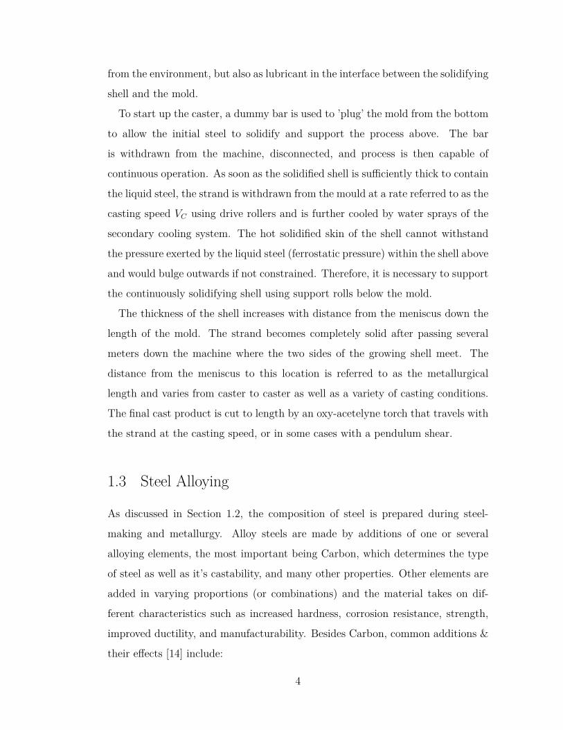
1.3 Steel Alloying

As discussed in Section 1.2, the composition of steel is prepared during steel-

making and metallurgy. Alloy steels are made by additions of one or several

alloying elements, the most important being Carbon, which determines the type

of steel as well as it’s castability, and many other properties. Other elements are

added in varying proportions (or combinations) and the material takes on dif-

ferent characteristics such as increased hardness, corrosion resistance, strength,

improved ductility, and manufacturability. Besides Carbon, common additions &

their effects [14] include:

4

Aluminum: Used as deoxidizer, restricts grain growth, helpful in nitriding

Chromium: Increased hardenability, toughness; and corrosion and wear resistance

Cobalt: Used in making cutting tools; improved hot hardness in ferrite

Manganese: Counteracts sulfur embrittlement, increased surface hardness & shock resistance

Molybdenum: Increases strength, resistance to shock and heat, higher creep strength

Nickel: Low temperature strength in pearlite and ferrite, Improves corrosion resistance

Phosphorus: Strengthen low C steels and can improve machinability

Silicon: Improved electrical properties, oxidation resistance, strengthen low alloy steels

Tungsten: Adds hardness, improves grain structure, and heat resistance

Vanadium: Grain refiner in austenite, increased strength, toughness and shock resistance

Other trace elements are always present in small amounts, and are often unin-

tended “residuals”; these include: Sulfur, Phosphorus, Silicon, Oxygen, Nitrogen,

Copper, Tin, Antimony, Bismuth, and a host of others.

For all of the ambient temperature benefits and performance gains that these

alloys provide to final steel products, addition of them to the steelmaking pro-

cess increases the complexity and makes it difficult to troubleshoot intermittent

problems, such as depressions and cracks during the continuous casting process.

Each company has their own offering of steel grades to meet the needs of cus-

tomer and industry demand, and decisions for grades to be cast are usually made

far in advance of the actual casting. Recent years have seen the appearance of

TRIP (TRansformation Induced Plasticity), TWIP (TWinning Induced Plastic-

ity), and AHSS (Advanced High Strength Steel) grades [15] in the market and

with their increased durability and strength, come a host of difficulties upstream

as their properties are not always fully understood. Due to this lack of fundamen-

tal knowledge, understanding the basic behavior of steel solidification as well as

observed trends is crucial to making decisions about casting conditions, especially

when it comes to new grades.

5

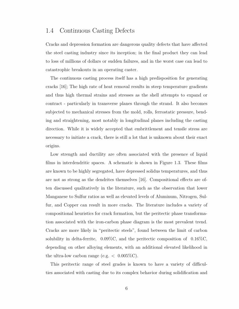
1.4 Continuous Casting Defects

Cracks and depression formation are dangerous quality defects that have affected

the steel casting industry since its inception; in the final product they can lead

to loss of millions of dollars or sudden failures, and in the worst case can lead to

catastrophic breakouts in an operating caster.

The continuous casting process itself has a high predisposition for generating

cracks [16]; The high rate of heat removal results in steep temperature gradients

and thus high thermal strains and stresses as the shell attempts to expand or

contract - particularly in transverse planes through the strand. It also becomes

subjected to mechanical stresses from the mold, rolls, ferrostatic pressure, bend-

ing and straightening, most notably in longitudinal planes including the casting

direction. While it is widely accepted that embrittlement and tensile stress are

necessary to initiate a crack, there is still a lot that is unknown about their exact

origins.

Low strength and ductility are often associated with the presence of liquid

films in interdendritic spaces. A schematic is shown in Figure 1.3. These films

are known to be highly segregated, have depressed solidus temperatures, and thus

are not as strong as the dendrites themselves [16]. Compositional effects are of-

ten discussed qualitatively in the literature, such as the observation that lower

Manganese to Sulfur ratios as well as elevated levels of Aluminum, Nitrogen, Sul-

fur, and Copper can result in more cracks. The literature includes a variety of

compositional heuristics for crack formation, but the peritectic phase transforma-

tion associated with the iron-carbon phase diagram is the most prevalent trend.

Cracks are more likely in “peritectic steels”, found between the limit of carbon

solubility in delta-ferrite, 0.09%C, and the peritectic composition of 0.16%C,

depending on other alloying elements, with an additional elevated likelihood in

the ultra-low carbon range (e.g. < 0.005%C).

This peritectic range of steel grades is known to have a variety of difficul-

ties associated with casting due to its complex behavior during solidification and

6

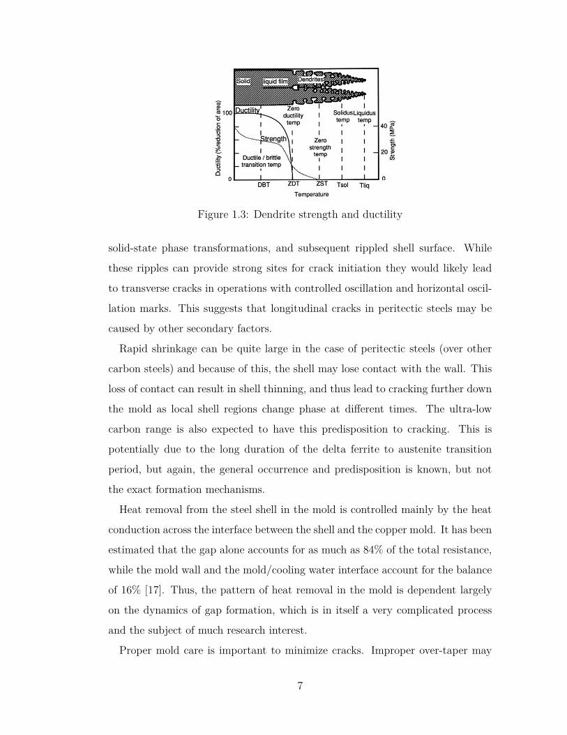
Figure 1.3: Dendrite strength and ductility

solid-state phase transformations, and subsequent rippled shell surface. While

these ripples can provide strong sites for crack initiation they would likely lead

to transverse cracks in operations with controlled oscillation and horizontal oscil-

lation marks. This suggests that longitudinal cracks in peritectic steels may be

caused by other secondary factors.

Rapid shrinkage can be quite large in the case of peritectic steels (over other

carbon steels) and because of this, the shell may lose contact with the wall. This

loss of contact can result in shell thinning, and thus lead to cracking further down

the mold as local shell regions change phase at different times. The ultra-low

carbon range is also expected to have this predisposition to cracking. This is

potentially due to the long duration of the delta ferrite to austenite transition

period, but again, the general occurrence and predisposition is known, but not

the exact formation mechanisms.

Heat removal from the steel shell in the mold is controlled mainly by the heat

conduction across the interface between the shell and the copper mold. It has been

estimated that the gap alone accounts for as much as 84% of the total resistance,

while the mold wall and the mold/cooling water interface account for the balance

of 16% [17]. Thus, the pattern of heat removal in the mold is dependent largely

on the dynamics of gap formation, which is in itself a very complicated process

and the subject of much research interest.

Proper mold care is important to minimize cracks. Improper over-taper may

7

push on the weak shell and distort it, this is more common towards mold exit.

Improper under-taper (usually occuring towards the middle of the mold) or im-

proper sub mold support can allow the strand to move around or bulge from

ferrostatic pressure. Irregular mold oscillation can result in deeper oscillation

marks or potentially slag getting stuck between the mold and shell. Mold wear is

known to change the taper over the life of the mold and if this is not accounted for

unintended bad taper practices may occur. Each of these mechanical mold issues

also mean deviation from uniform heat transfer, this can cause local reheating

and weakening of the shell. This reheating is significant for a number of reasons

not just related to the strength of the material. If the temperature change is

significant enough a phase transformation may take place, meaning not only a

thinner shell is present, but in the case of reheating from austenite, the potential

appearance of a weak delta ferrite phase surrounded by colder and much stronger

austenite.

Much of the contemporary literature is concerned with the micro-scale and

compositional phenomena related to cracking. This is good on a fundamental

level and a complete understanding will expand the tools we have to fix such

issues, however, it does leave many unanswered questions. We know compositional

differences are known to have a strong effect on crack susceptibility, but we know

little about the differences in cause: Is the physical mechanism that is responsible

for peritectic cracking, the same as that of the ultra-low carbon steel? Cracks are

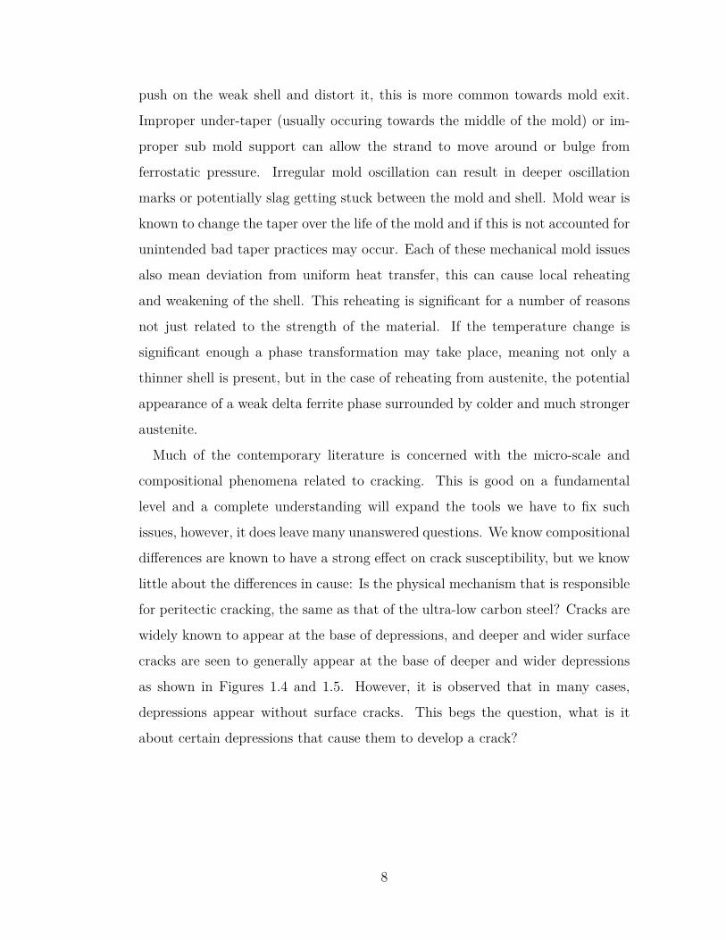
widely known to appear at the base of depressions, and deeper and wider surface

cracks are seen to generally appear at the base of deeper and wider depressions

as shown in Figures 1.4 and 1.5. However, it is observed that in many cases,

depressions appear without surface cracks. This begs the question, what is it

about certain depressions that cause them to develop a crack?

8

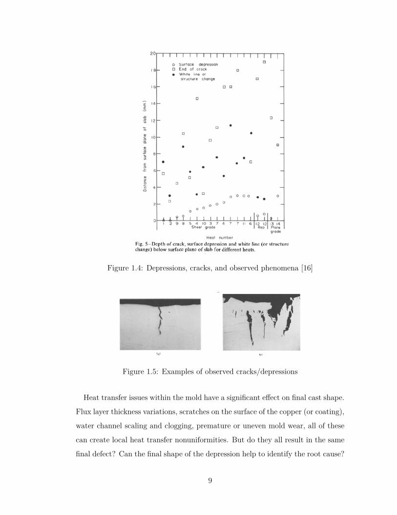
Figure 1.4: Depressions, cracks, and observed phenomena [16]

Figure 1.5: Examples of observed cracks/depressions

Heat transfer issues within the mold have a significant effect on final cast shape.

Flux layer thickness variations, scratches on the surface of the copper (or coating),

water channel scaling and clogging, premature or uneven mold wear, all of these

can create local heat transfer nonuniformities. But do they all result in the same

final defect? Can the final shape of the depression help to identify the root cause?

9

How large can a mold scratch be before we begin to see indications on the slab?

How do flux thickness variations translate to the final shell?

Cracks and depressions are still one of the most costly defects in continuous

casting, many times resulting in resurfacing, scarfing, downgrading, or complete

scrapping. As technology has increased so too has our ability to limit and confine

our defects to smaller sizes, and less detrimental areas. However, cracks remain

an issue at many casters and while general causes are known, little is known

(and proven) on the process of formation. Much of the knowledge that does

exist is empirical, and there is quite a bit still unknown about the fundamental

mechanisms; as such more work is needed on the steps that can be taken when

troubleshooting a caster that is producing a high amounts of them.

1.5 Objectives of Current Work

While the continuous casting process, and steelmaking in general, is one of the old-

est processes of the industrialized world, it is clear that its complexities are vast.

As industrial experience and research budgets increase in continuous casting, im-

provements are seen across the board. Previous advances have mainly come from

trials at operating steel plants. But, as the process improves, and defects become

more intermittent, this “trial and error” approach becomes more expensive. With

continuous casting production measured in the billions of metric tonnes per year,

any small improvement in the process leads to increases in throughput, efficiency,

and cost savings.

Modeling, more specifically computational modeling, allows engineers to take

a unique real world situation, make assumptions, and distill it into its most rele-

vant and basic parameters. Computational modeling affects our lives daily from

weather forecasts to traffic patterns and power grid operations. By making these

simplifications we can study and begin to understand the phenomena and be-

havior in different situations that might otherwise be extremely expensive or un-

realistic to duplicate in the real world. Continuous casting research stands to

10

benefit greatly from computational modeling as the real process environment is

so hazardous that conventional experimental techniques are often inadequate and

dangerous at the temperatures and conditions that are present at an operating

caster.

This work aims to take initial steps towards the ultimate goal of fundamental

understanding of crack formation and to evaluate the differences of how stress and

strain develop between steel grades. This will provide knowledge towards better

understanding of how cracks and depressions form, and assist in troubleshooting

and preventing them, and within these tools and understanding, examining the

effect of steel grade on that behavior.

This thesis is divided into 3 chapters which follow this introduction. First, a

mathematical model is presented and applied to examine the thermal-mechanical

solidification behavior of 4 different steel grades utilizing grade- and temperature-

dependent properties. This model is used to explore the behaviors that result from

the different phase transformation histories in commercially cast steels, with uni-

form solidification of a plate as a starting point. Then, a temperature-dependent

thermal resistor model of the interfacial gap is proposed and demonstrated to

allow for coupled thermal and stress modeling. In addition it introduces the op-

portunity to alter the heat flux profile throughout the entire mold. In this way

we can examine the effect of uniform and nonuniform flux thickness variations

Imposed air gaps, slag fingers, and a variety of other potential mold scenarios.

Finally, the coupled thermal stress model is used to simulate a flux layer thick-

ness variation and the formation of a depression during continuous casting in the

model.

11

Chapter 2

Steel Grade Effects On Solidification Behavior

2.1 Abstract

A mathematical model has been developed, using ABAQUS finite element soft-

ware [18], to study the effect of grade on temperature, stress, strain, and shell

development early in the solidification process of continuously cast steels and

use it to help design continuous casting taper profiles for different steels. This

work investigates the effect of grade on thermal-mechanical behavior during ini-

tial solidification of steels during continuous casting of a wide strand. The em-

ployed finite-element model uses an efficient algorithm to integrate the nonlinear

temperature- and phase-dependent elastic-viscoplastic constitutive equations [19].

The model is validated using an analytical solution, and a mesh convergence study

is performed. Four steel grades are simulated for 30 s of casting without friction:

Ultra-Low Carbon (0.003%C), Low Carbon (0.04%C), Peritectic (0.13%C), and

High Carbon (0.47%C). All grades show the same general behavior. Initially, fast

cooling causes tensile stress and inelastic strain near the surface of the shell, with

slight complementary compression beneath the surface, especially with lower car-

bon content. As the cooling rate decreases with time, the surface quickly reverses

into compression, with a tensile region developing towards the solidification front.

Higher stress and inelastic strain are generated in the high carbon steels, because

they contain more high-strength austenite. Stress in the δ-ferrite phase near the

solidification is always very small, owing to the low strength of this phase. The

total strain remains uniform through the thickness, and becomes increasingly neg-

ative at a decreasing rate as the dwell time increases. After a great amount of

12

shrinkage in the first few seconds, the shell shrinks at a decreasing rate, which

was used to calculate grade-specific ideal taper profiles. All grades follow a simi-

lar, roughly parabolic shape, except for the peritectic, which was either larger or

smaller, depending on the heat transfer.

2.2 Introduction

The surface quality of cast metal products depends significantly on initial solidifi-

cation behavior. In casting processes, such as continuous casting, die casting and

ingot casting, defects such as cracks, segregation, porosity, and microstructural

or grain defects that appear in the newly-solidified shell may evolve and lead to

problems in the final product, even after many subsequent processing steps.

Steel composition strongly affects the surface quality of continuously cast steels,

especially for grades involving the peritectic transformation. In addition, each

steel grade has slightly different shell growth, shrinkage, and thermal-mechanical

characteristics. Fundamental understanding of these phenomena is especially re-

quired when developing and solving problems in new steel grades, such as Ad-

vanced High Strength Steels (AHSS). The extreme environment of steel casting

processes makes experimentation difficult. Thus, modeling is an important tool

in the development of this understanding.

The thermal and mechanical behavior of the solidifying shell is explored in this

work using a computational model. Four steel grades are studied to explore the

typical behavior of four different types of phase transformation histories in the

iron-rich side of the Fe − Fe3C phase diagram: ultra-low carbon (ULC) with

0.003 wt. %C, low carbon (LC) with 0.045 wt. %C, peritectic (P) with 0.13 wt.

%C, and high-carbon (HC) with 0.47 wt. %C.

13

2.2.1 Literature Review

In preparation for this work, a literature review was conducted to examine the

state-of-the-art and identify potential gaps in knowledge. Previous studies have

often focused on the effect of steel grade on micro-scale behavior such as the

formation of dendrites during solidification [20–24], segregation [20, 25–30], the

columnar-to-equiaxed transition [22, 29, 31–33], and damage criteria for hot tear

crack formation [34–37]. Other studies have examined macroscopic scale behavior,

such as shell growth [38–40], shell shrinkage [41, 42], solidification force [43, 44],

stress development [45,46], hot ductility [26,47–49], and strain to failure [50].

Small differences in steel composition can greatly change evolution of the phase

fractions during solidification [26, 51], and consequent changes in the material

properties and behaviors. Specifically, ultra-low carbon steels and peritectic steels

experience much greater mechanical deformation during solidification than do low-

and medium carbon steels, which consequently causes lower and less-uniform heat

transfer [52], and greater crack susceptibility for peritectics [39,53,54]. Identifying

phase fraction histories is a useful step in predicting these phenomena. Tools to

study the equilibrium phases of steels have used experimental methods involving

slow cooling rates, such as Differential Scanning Calorimetry [55, 56], as well as

steel-composition-dependent phase diagrams [30, 57], and applying free-energy-

based models, such as Thermocalc and Factsage to steel [58–60]. Some tools,

such as IDS, model species diffusion to incorporate non-equilibrium kinetic effects

in finding the phase fractions [27].

Steel properties at high temperature are difficult to measure; only a few papers

have measured thermal properties [61,62] or mechanical testing in the appropriate

regime of low-strain (< 2 %), and low-strain-rate (10−5 to 10−2 %/s), which

include tensile tests on austenite and ferrite [48, 63] and creep tests above 800◦C

[40].

Previous macro-scale thermal-mechanical modeling work [41,46,64–73] has been

conducted using temperature-dependent constitutive and material properties in-

14

cluding studies for billets [41,67–71], slabs [41,72], as well as work towards better

taper prediction [41,46,66,67,71–73].

Other models have used phase field modeling which include studies on hot tear

sensitivity [51, 74] and microstructure evolution [75, 76]. Only a few previous

models have investigated the effect of steel grade on initial solidification, such as

the deformed shape of solidifying droplets [77] or continuously-cast shells [65].

The current work models the macroscale thermal-mechanical behavior during

the initial solidification of a steel casting process; it presents validation using

an analytical solution, and then applies the model to explore the fundamental

differences between steel grades, in the context of a typical continuous steel casting

process.

2.3 Goals

While the literature supplies useful tools for understanding some of the expected

behavior, these previous models have been applied to varying steel grades but in

a limited manner and not with differences in grade behavior being the primary

focus. This work demonstrates the methodology necessary to model and capture

the relevant behavior in a solidification problem; it also explores the basic property

differences between steel grades, presents validation using analytical solutions, and

a simulation of a continuous thin slab steel casting process where the shrinkage

and solidification behavior of each grade is explored. In addition, we show a

comparison of stress and strain profiles for each grade with the same interfacial

heat flux profile.

As peritectic steel grades are widely accepted to be highly complex and are the

subject of significant study in the literature [53,78–80] as well as current industrial

interest, this work includes one to study general behavior, with the understanding

it is not all encompassing and the intent that further study be included in the

future. The peritectic grade in this work is also examined using a lower applied

heat flux to simulate more appropriate casting conditions.

15

With the information this model provides, better choices can be made for taper

profiles and casting conditions when attempting to cast grades where complete

information may not exist. In addition, it is the first step in demonstrating a

transient 3-D model of thermal-mechanical behavior where the correct behavior

can be verified in a simplified case where an analytical solution exists, while

allowing for extensions to higher dimensional modeling work.

2.4 Model Description

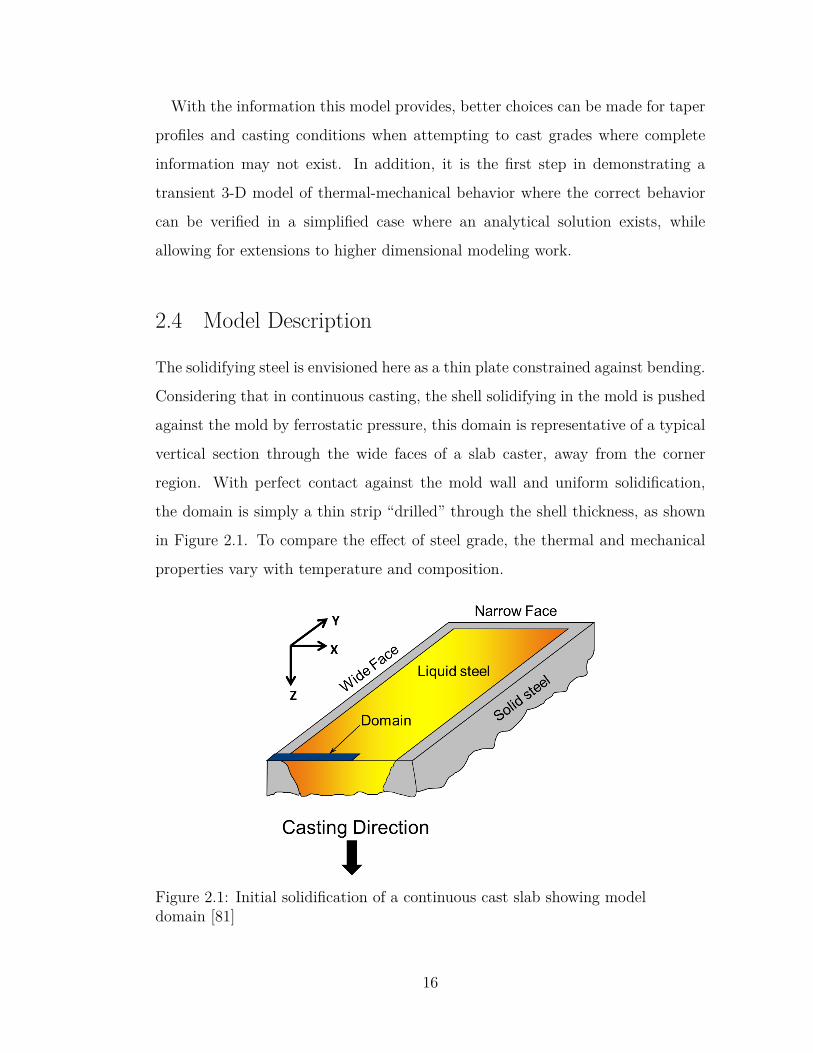
The solidifying steel is envisioned here as a thin plate constrained against bending.

Considering that in continuous casting, the shell solidifying in the mold is pushed

against the mold by ferrostatic pressure, this domain is representative of a typical

vertical section through the wide faces of a slab caster, away from the corner

region. With perfect contact against the mold wall and uniform solidification,

the domain is simply a thin strip “drilled” through the shell thickness, as shown

in Figure 2.1. To compare the effect of steel grade, the thermal and mechanical

properties vary with temperature and composition.

Figure 2.1: Initial solidification of a continuous cast slab showing modeldomain [81]

16

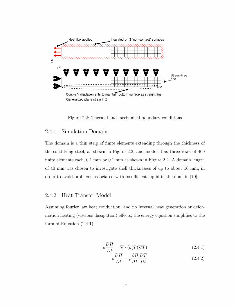
Figure 2.2: Thermal and mechanical boundary conditions

2.4.1 Simulation Domain

The domain is a thin strip of finite elements extending through the thickness of

the solidifying steel, as shown in Figure 2.2, and modeled as three rows of 400

finite elements each, 0.1 mm by 0.1 mm as shown in Figure 2.2. A domain length

of 40 mm was chosen to investigate shell thicknesses of up to about 16 mm, in

order to avoid problems associated with insufficient liquid in the domain [70].

2.4.2 Heat Transfer Model

Assuming fourier law heat conduction, and no internal heat generation or defor-

mation heating (viscious dissipation) effects, the energy equation simplifies to the

form of Equation (2.4.1).

ρDH

Dt= ∇ · (k(T )∇T ) (2.4.1)

ρDH

Dt= ρ

∂H

∂T

DT

Dt(2.4.2)

17

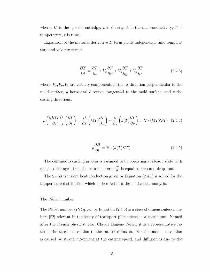
where, H is the specific enthalpy, ρ is density, k is thermal conductivity, T is

temperature, t is time.

Expansion of the material derivative D term yields independent time tempera-

ture and velocity terms:

DT

Dt= ∂T

∂t+ Vx

∂T

∂x+ Vy

∂T

∂y+ Vz

∂T

∂z(2.4.3)

where, Vx, Vy, Vz are velocity components in the: x direction perpendicular to the

mold surface, y horizontal direction tangential to the mold surface, and z the

casting directions.

ρ

(∂H(T )∂T

)(∂T

∂t

)= ∂

∂x

(k(T )∂T

∂x

)+ ∂

∂y

(k(T )∂T

∂y

)= ∇ · (k(T )∇T ) (2.4.4)

ρ∂H

∂t= ∇ · (k(T )∇T ) (2.4.5)

The continuous casting process is assumed to be operating at steady state with

no speed changes, thus the transient term ∂T∂t

is equal to zero and drops out.

The 2−D transient heat conduction given by Equation (2.4.1) is solved for the

temperature distribution which is then fed into the mechanical analysis.

The Péclet number

The Péclet number (Pe) given by Equation (2.4.6) is a class of dimensionless num-

bers [82] relevant in the study of transport phenomena in a continuum. Named

after the French physicist Jean Claude Eugène Péclet, it is a representative ra-

tio of the rate of advection to the rate of diffusion. For this model, advection

is caused by strand movement at the casting speed, and diffusion is due to the

18

thermal diffusivity of the steel given by Equation (2.4.7).

Pe = Lu

α(2.4.6)

where α is thermal diffusivity, L is a characteristic length, u is characteristic

velocity,

α = k

ρcp(2.4.7)

thus,

Pe = Lukρcp

(2.4.8)

Substituting Equation (2.4.8) with casting parameters, it becomes:

Pe = LVCkρcp

(2.4.9)

Where L is the distance below the meniscus taken below as mold exit, Vc is the

casting speed, k is the thermal conductivity, ρ is the mass density, and Cp is the

specific heat capacity.

VC = 3m min−1 L = 1m

k = 33W m−1 K ρ = 7500kg m−3

Cp = 661J kg−1 K Hf = 272kJ kg−1

∆T = 500◦C

19

The assumption of advection domination can be seen, even for very short times.

Even for casting speeds as low as 1 m min−1 by 0.25 seconds, advection is already

3 orders of magnitude greater than conduction by mold exit. This time below

meniscus directly translates to the distance below meniscus as a result of the

constant casting speed.

Pe = LVc(kρcp

) = 1(m)× 3(m/min)33(w/m×K)

7500(kg/m3)×661(J/kg×K)

= 7.5× 103 (2.4.10)

With negligible heat conduction in the casting direction, a Lagrangian domain

may be used to analyze the heat transfer in the solidifying shell. This approxi-

mation essentially transforms the physical z - direction into a temporal quantity,

which is valid while the process remains at steady state.

2.4.3 Stress Model

During initial solidification the thermal-mechanical strains are on the order of

only a few percent. Thus, the small strain assumption was adopted for this work.

This assumption is supported by previous solidification model results [83].

∇ · σ + b = 0 (2.4.11)

The general governing equation for the static problem is given by the force

equilibrium balance in Equation (2.4.11), where σ is the second order Cauchy

stress tensor, and b is an applied traction.

The out-of-plane (z-direction) stress is characterized by a state of generalized

plane strain, where slices are constrained to remain planar by continuity. The

lower edge is also constrained to remain planar using an ABAQUS assembly EQN

defined in the input file, shown in Appendix B.3.2.

20

2.4.4 Liquid Treatment

Solidification problems present a unique challenge when it comes to handling the

liquid. Liquid that is modeled as too weak (very small yield strength if considered

to act like a Bingham plastic [84]) or the presence of too much of it in the domain

(not taking full advantage of symmetry or areas of interest) can be difficult to

converge if at all. Conversely, liquid that is modeled as too strong (with a high

yield strength) will converge but may yield non-physical behavior such as not

allowing the solid to shrink as it would naturally.

For this work the liquid region was treated as a perfectly plastic solid [85].

The yield strength for the liquid was chosen to be σyield = 10 kPa. This value

was chosen to provide a minimum strength needed to aid in convergence without

adding inappropriate strength to the liquid based on studies conducted varying

this parameter. This behavior is applied any time the mass fraction of the liquid

is greater than zero.

2.4.5 Model Setup

The initial temperature of the domain for each case is set 5◦C above the grade’s

liquidus temperature to facilitate comparison between them. This superheat rep-

resents a steady fluid flow in the meniscus region and is in line with predicted

meniscus temperature profiles reported in the literature [86].

While fluid flow within the liquid pool may create a non-uniform superheat

distribution in the melt, the effect is minor when the pouring temperature is close

to liquidus temperature; and thus is ignored in this work, which treats superheat

in the liquid with simple conduction [64].

Contact with the mold (and resultant frictional effects) have been neglected and

the model does not include applied ferrostatic pressure, so in the stress equilibrium

equation for this work b = 0. Instead the contact interface has been constrained

against rigid body motion as shown in Figure 2.2.

To ensure that an accurate solution was being obtained, a mesh resolution study

21

was conducted to select the mesh refinement level and 400 elements through the

thickness were used. Details of this study can be found in Section 2.8.2.

2.5 Heat Flux

In a continuous caster, the instantaneous rate of heat leaving the surface of the

solidifying steel shell (heat flux), q̇Inst MW m−2, can be estimated as a function of

time down the mold, t, by thermocouples embedded in the mold wall. In addition,

the average heat flux leaving the mold q̇Avg MW m−2 can be found by measuring

the rise in temperature and flow rate of the cooling water, and knowing the surface

area of the mold in contact with the steel. This average can be converted to the

total heat removed, Q̄Tot MW m−2, during the “dwell time”, tdwell, spent by the

steel in the mold:

Q̄Tot = q̇Avg × tdwell (2.5.1)

where,

tdwell = zdwellVc

(2.5.2)

zdwell is working mold length, and Vc is casting speed, assumed to be constant.

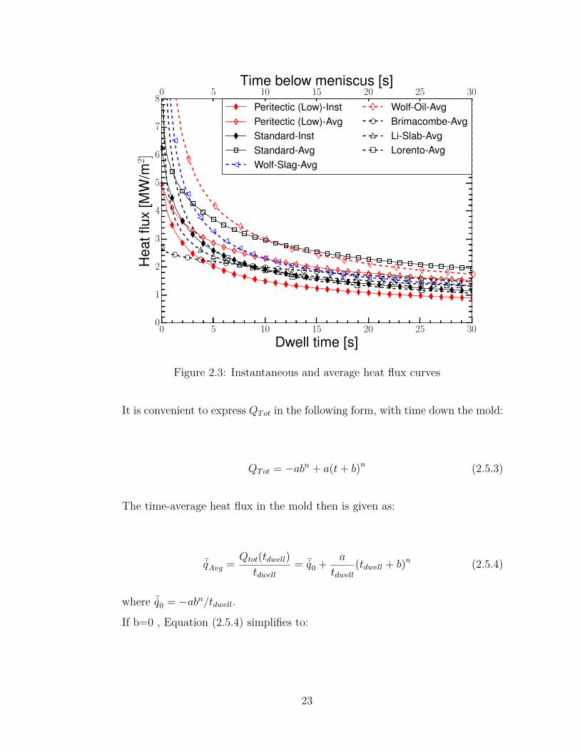
Measurements of total mold heat removal, Q̄Tot , from previous work [68, 69, 69,

87–92] are plotted vs dwell time in Figure 2.3.

22

0 5 10 15 20 25 30

Dwell time [s]0

1

2

3

4

5

6

7

8

Hea

tflux

[MW

/m2 ]

Peritectic (Low)-InstPeritectic (Low)-AvgStandard-InstStandard-AvgWolf-Slag-Avg

Wolf-Oil-AvgBrimacombe-AvgLi-Slab-AvgLorento-Avg

0 5 10 15 20 25 30Time below meniscus [s]

Figure 2.3: Instantaneous and average heat flux curves

It is convenient to express QTot in the following form, with time down the mold:

QTot = −abn + a(t+ b)n (2.5.3)

The time-average heat flux in the mold then is given as:

¯̇qAvg = Qtot(tdwell)tdwell

= ¯̇q0 + a

tdwell(tdwell + b)n (2.5.4)

where ¯̇q0 = −abn/tdwell.

If b=0 , Equation (2.5.4) simplifies to:

23

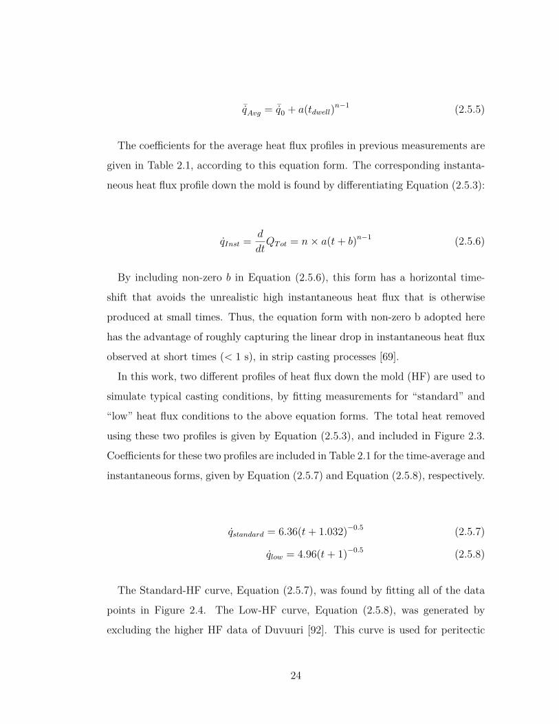
¯̇qAvg = ¯̇q0 + a(tdwell)n−1 (2.5.5)

The coefficients for the average heat flux profiles in previous measurements are

given in Table 2.1, according to this equation form. The corresponding instanta-

neous heat flux profile down the mold is found by differentiating Equation (2.5.3):

q̇Inst = d

dtQTot = n× a(t+ b)n−1 (2.5.6)

By including non-zero b in Equation (2.5.6), this form has a horizontal time-

shift that avoids the unrealistic high instantaneous heat flux that is otherwise

produced at small times. Thus, the equation form with non-zero b adopted here

has the advantage of roughly capturing the linear drop in instantaneous heat flux

observed at short times (< 1 s), in strip casting processes [69].

In this work, two different profiles of heat flux down the mold (HF) are used to

simulate typical casting conditions, by fitting measurements for “standard” and

“low” heat flux conditions to the above equation forms. The total heat removed

using these two profiles is given by Equation (2.5.3), and included in Figure 2.3.

Coefficients for these two profiles are included in Table 2.1 for the time-average and

instantaneous forms, given by Equation (2.5.7) and Equation (2.5.8), respectively.

q̇standard = 6.36(t+ 1.032)−0.5 (2.5.7)

q̇low = 4.96(t+ 1)−0.5 (2.5.8)

The Standard-HF curve, Equation (2.5.7), was found by fitting all of the data

points in Figure 2.4. The Low-HF curve, Equation (2.5.8), was generated by

excluding the higher HF data of Duvuuri [92]. This curve is used for peritectic

24

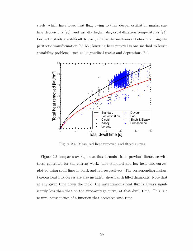
steels, which have lower heat flux, owing to their deeper oscillation marks, sur-

face depressions [93], and usually higher slag crystallization temperatures [94].

Peritectic steels are difficult to cast, due to the mechanical behavior during the

peritectic transformation [53, 55]; lowering heat removal is one method to lessen

castability problems, such as longitudinal cracks and depressions [54].

0 5 10 15 20 25 30

Total dwell time [s]0

10

20

30

40

50

60

Tota

lhea

trem

oved

[MJ/

m2 ]

StandardPeritectic (Low)CicuttiKapajLorento

DuvuuriParkSingh & BlazekBrimacombe

Figure 2.4: Measured heat removed and fitted curves

Figure 2.3 compares average heat flux formulas from previous literature with

those generated for the current work. The standard and low heat flux curves,

plotted using solid lines in black and red respectively. The corresponding instan-

taneous heat flux curves are also included, shown with filled diamonds. Note that

at any given time down the mold, the instantaneous heat flux is always signif-

icantly less than that on the time-average curve, at that dwell time. This is a

natural consequence of a function that decreases with time.

25

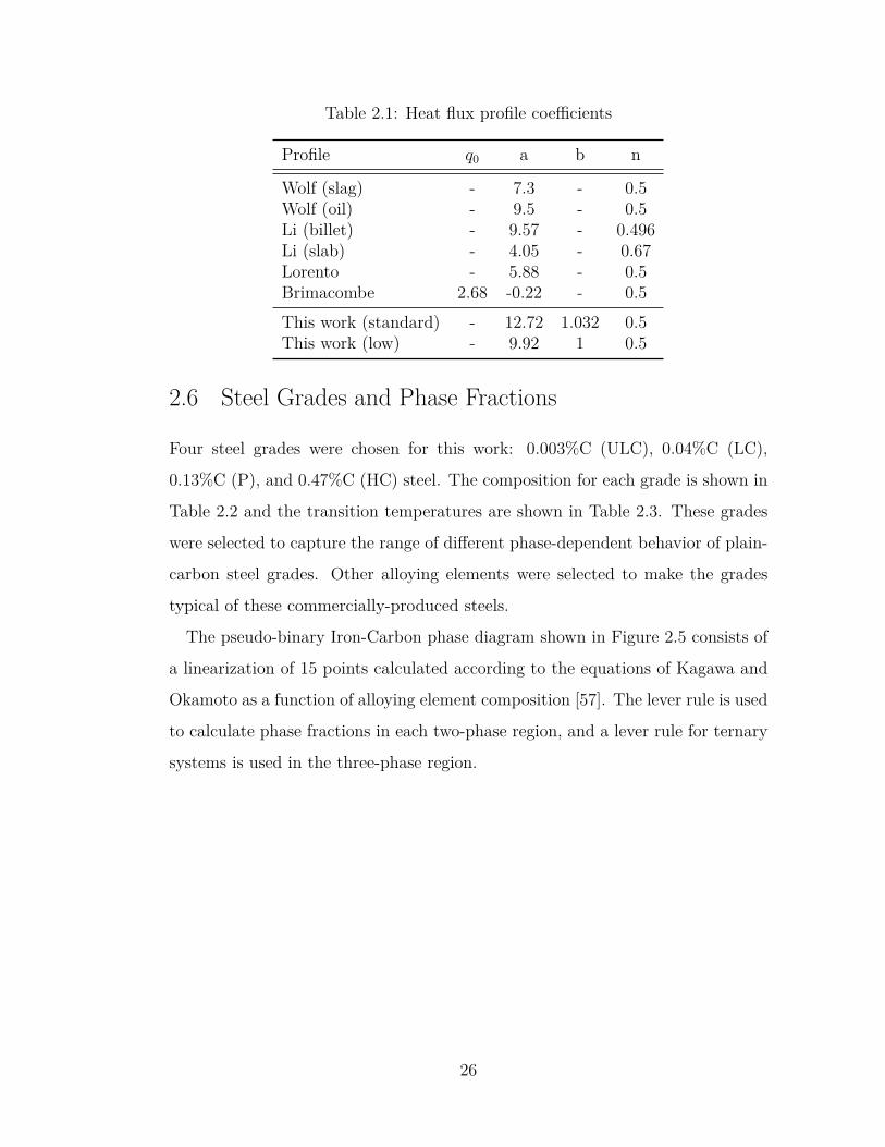
Table 2.1: Heat flux profile coefficients

Profile q0 a b n

Wolf (slag) - 7.3 - 0.5Wolf (oil) - 9.5 - 0.5Li (billet) - 9.57 - 0.496Li (slab) - 4.05 - 0.67Lorento - 5.88 - 0.5Brimacombe 2.68 -0.22 - 0.5This work (standard) - 12.72 1.032 0.5This work (low) - 9.92 1 0.5

2.6 Steel Grades and Phase Fractions

Four steel grades were chosen for this work: 0.003%C (ULC), 0.04%C (LC),

0.13%C (P), and 0.47%C (HC) steel. The composition for each grade is shown in

Table 2.2 and the transition temperatures are shown in Table 2.3. These grades

were selected to capture the range of different phase-dependent behavior of plain-

carbon steel grades. Other alloying elements were selected to make the grades

typical of these commercially-produced steels.

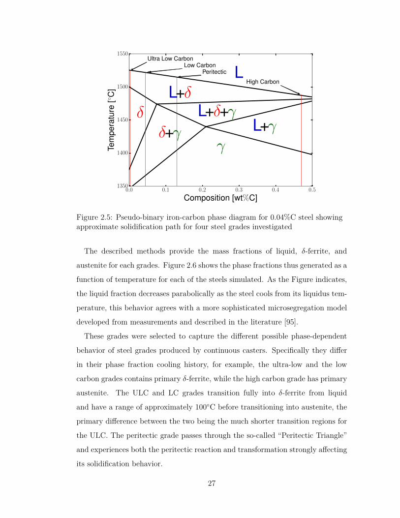
The pseudo-binary Iron-Carbon phase diagram shown in Figure 2.5 consists of

a linearization of 15 points calculated according to the equations of Kagawa and

Okamoto as a function of alloying element composition [57]. The lever rule is used

to calculate phase fractions in each two-phase region, and a lever rule for ternary

systems is used in the three-phase region.

26

0.0 0.1 0.2 0.3 0.4 0.5

Composition [wt%C]

1350

1400

1450

1500

1550

Tem

pera

ture

[◦C

]

L

δ

γδ+γ

L+δ+γL+δ

L+γ

Ultra Low CarbonLow Carbon

Peritectic

High Carbon

Figure 2.5: Pseudo-binary iron-carbon phase diagram for 0.04%C steel showingapproximate solidification path for four steel grades investigated

The described methods provide the mass fractions of liquid, δ-ferrite, and

austenite for each grades. Figure 2.6 shows the phase fractions thus generated as a

function of temperature for each of the steels simulated. As the Figure indicates,

the liquid fraction decreases parabolically as the steel cools from its liquidus tem-

perature, this behavior agrees with a more sophisticated microsegregation model

developed from measurements and described in the literature [95].

These grades were selected to capture the different possible phase-dependent

behavior of steel grades produced by continuous casters. Specifically they differ

in their phase fraction cooling history, for example, the ultra-low and the low

carbon grades contains primary δ-ferrite, while the high carbon grade has primary

austenite. The ULC and LC grades transition fully into δ-ferrite from liquid

and have a range of approximately 100◦C before transitioning into austenite, the

primary difference between the two being the much shorter transition regions for

the ULC. The peritectic grade passes through the so-called “Peritectic Triangle”

and experiences both the peritectic reaction and transformation strongly affecting

its solidification behavior.

27

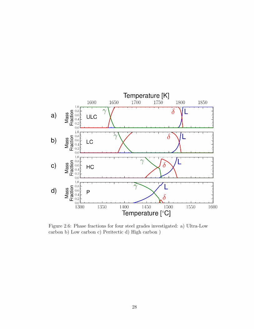
Figure 2.6: Phase fractions for four steel grades investigated: a) Ultra-Lowcarbon b) Low carbon c) Peritectic d) High carbon )

28

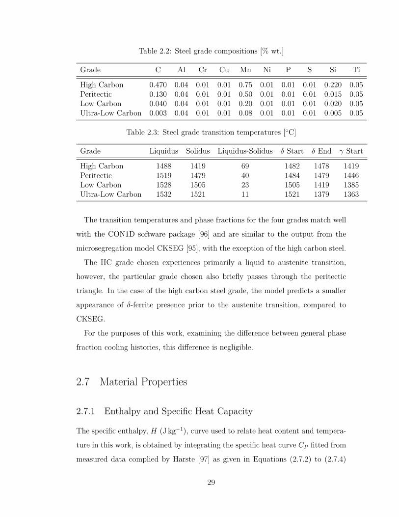
Table 2.2: Steel grade compositions [% wt.]

Grade C Al Cr Cu Mn Ni P S Si Ti

High Carbon 0.470 0.04 0.01 0.01 0.75 0.01 0.01 0.01 0.220 0.05Peritectic 0.130 0.04 0.01 0.01 0.50 0.01 0.01 0.01 0.015 0.05Low Carbon 0.040 0.04 0.01 0.01 0.20 0.01 0.01 0.01 0.020 0.05Ultra-Low Carbon 0.003 0.04 0.01 0.01 0.08 0.01 0.01 0.01 0.005 0.05

Table 2.3: Steel grade transition temperatures [◦C]

Grade Liquidus Solidus Liquidus-Solidus δ Start δ End γ Start

High Carbon 1488 1419 69 1482 1478 1419Peritectic 1519 1479 40 1484 1479 1446Low Carbon 1528 1505 23 1505 1419 1385Ultra-Low Carbon 1532 1521 11 1521 1379 1363

The transition temperatures and phase fractions for the four grades match well

with the CON1D software package [96] and are similar to the output from the

microsegregation model CKSEG [95], with the exception of the high carbon steel.

The HC grade chosen experiences primarily a liquid to austenite transition,

however, the particular grade chosen also briefly passes through the peritectic

triangle. In the case of the high carbon steel grade, the model predicts a smaller

appearance of δ-ferrite presence prior to the austenite transition, compared to

CKSEG.

For the purposes of this work, examining the difference between general phase

fraction cooling histories, this difference is negligible.

2.7 Material Properties

2.7.1 Enthalpy and Specific Heat Capacity

The specific enthalpy, H (J kg−1), curve used to relate heat content and tempera-

ture in this work, is obtained by integrating the specific heat curve CP fitted from

measured data complied by Harste [97] as given in Equations (2.7.2) to (2.7.4)

29

1000 1100 1200 1300 1400 1500 1600

Temperature [◦C]0

5000

10000

15000

20000

25000

30000

35000

40000

Spe

cific

Hea

t[kJ

kgK

]

Ultra-Low Carbon (0.003 %)Low Carbon (0.03 %)Peritectic (0.13 %)High Carbon (0.47 %)

1300 1400 1500 1600 1700 1800Temperature [K]

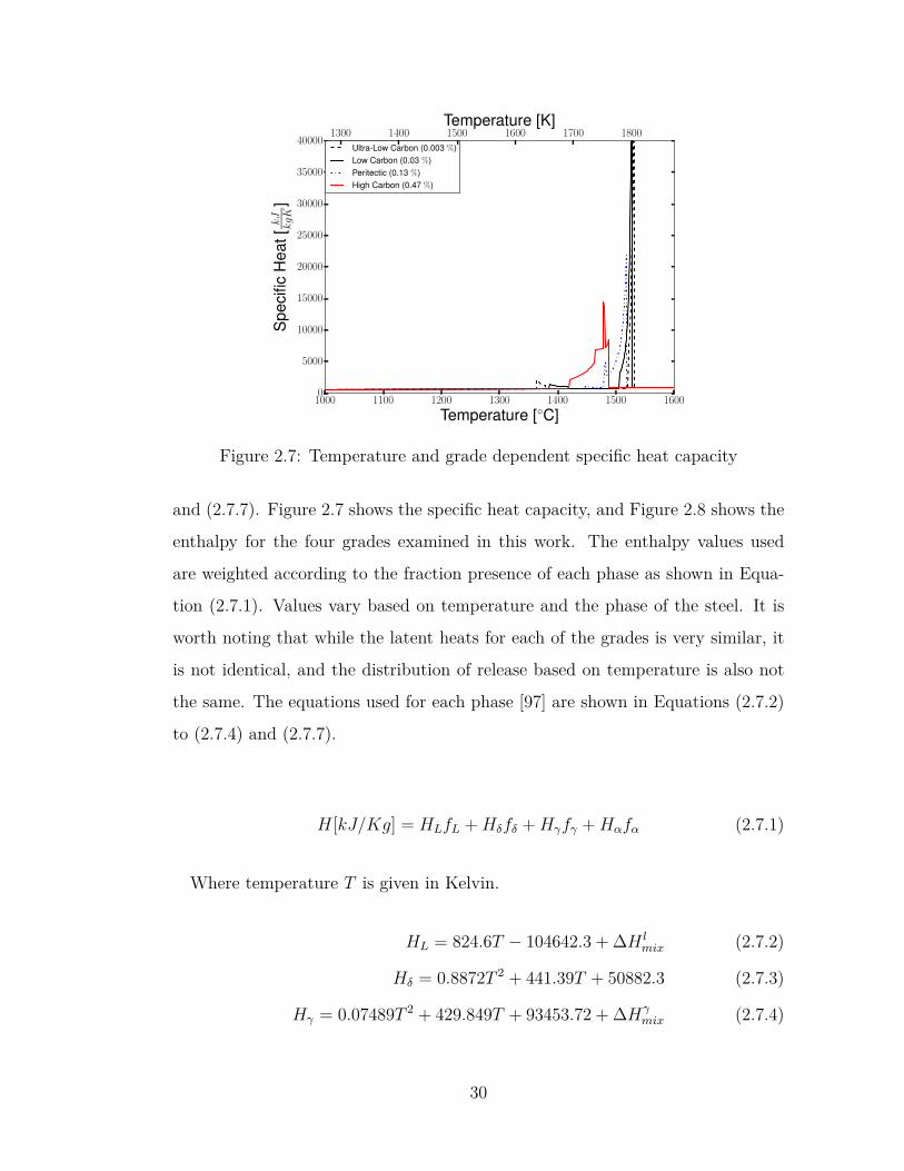
Figure 2.7: Temperature and grade dependent specific heat capacity

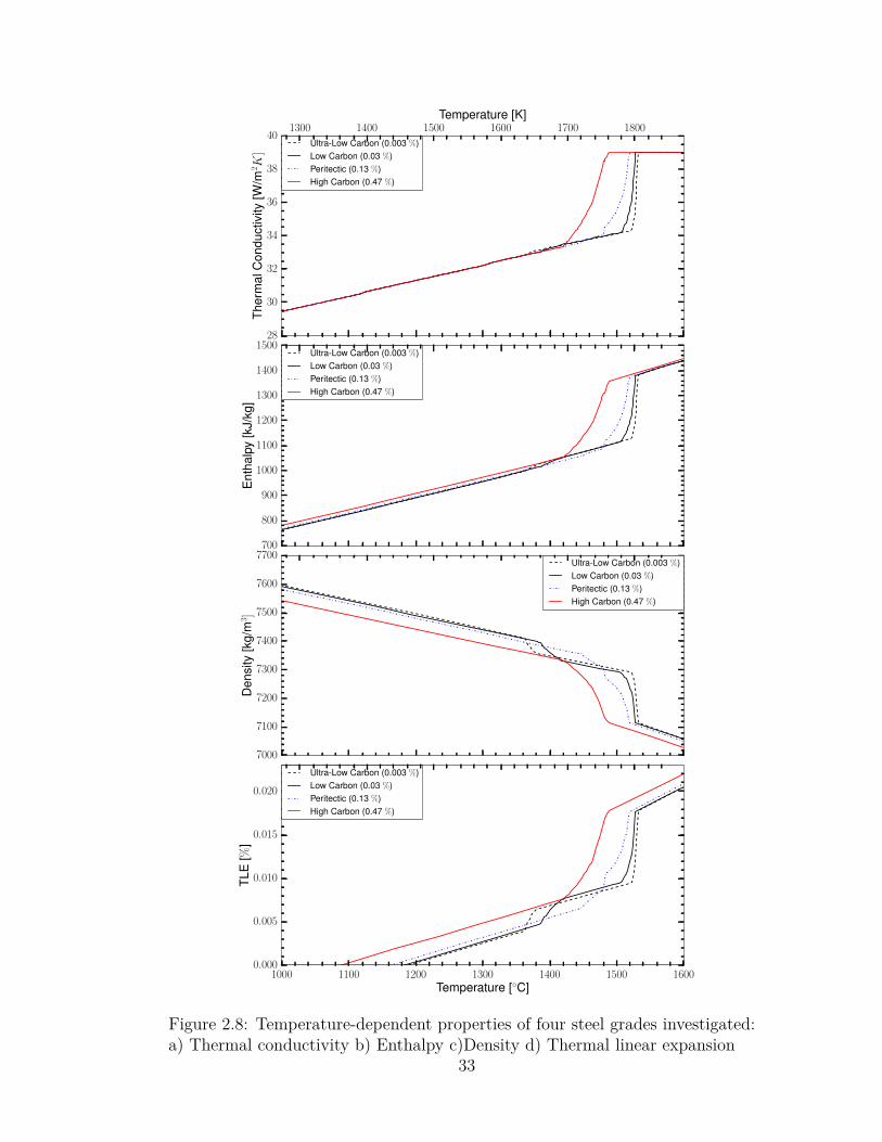
and (2.7.7). Figure 2.7 shows the specific heat capacity, and Figure 2.8 shows the

enthalpy for the four grades examined in this work. The enthalpy values used

are weighted according to the fraction presence of each phase as shown in Equa-

tion (2.7.1). Values vary based on temperature and the phase of the steel. It is

worth noting that while the latent heats for each of the grades is very similar, it

is not identical, and the distribution of release based on temperature is also not

the same. The equations used for each phase [97] are shown in Equations (2.7.2)

to (2.7.4) and (2.7.7).

H[kJ/Kg] = HLfL +Hδfδ +Hγfγ +Hαfα (2.7.1)

Where temperature T is given in Kelvin.

HL = 824.6T − 104642.3 + ∆H lmix (2.7.2)

Hδ = 0.8872T 2 + 441.39T + 50882.3 (2.7.3)

Hγ = 0.07489T 2 + 429.849T + 93453.72 + ∆Hγmix (2.7.4)

30

where,

∆H lmix = 18125(%C) + 1966120 (%C)2

43.839(%C) + 1201.1 (2.7.5)

∆Hγmix = 36601(%C) + 1907930 (%C)2

43.839(%C) + 1201.1 (2.7.6)

Hα =

5188T−1 − 86 + 0.505T

−6.55× 10−5T 2 + 1.5× 10−7T 3 T ≤ 800

5188T−1 − 86 + 0.505T

−6.55× 10−5T 2 + 1.5× 10−7T 3 800 < T ≤ 1000

5188T−1 − 86 + 0.505T

−6.55× 10−5T 2 + 1.5× 10−7T 3 1000 < T ≤ 1042

5188T−1 − 86 + 0.505T

−6.55× 10−5T 2 + 1.5× 10−7T 3 1042 < T ≤ 1060

−10.068T + 2.9934× 10−3T 2

−5.21766× 106T−1 + 12.822 1060 < T ≤ 1184

(2.7.7)

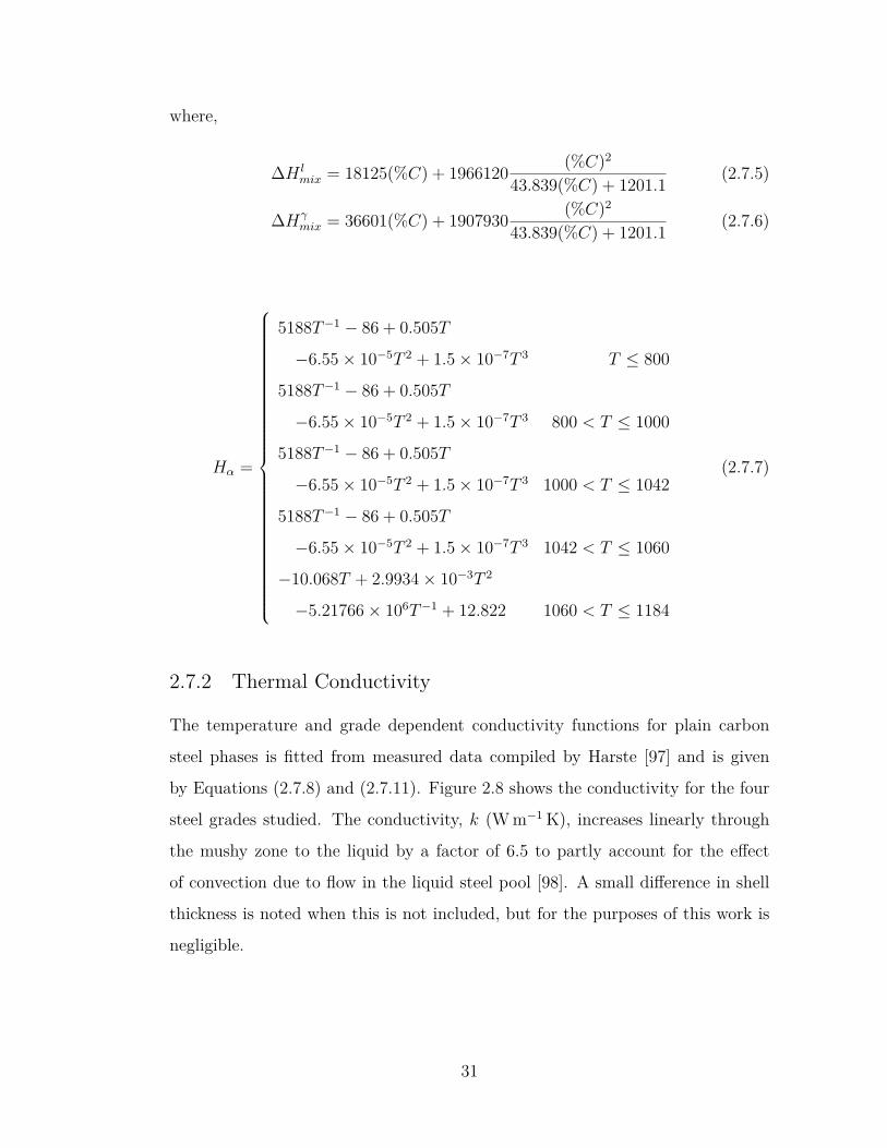
2.7.2 Thermal Conductivity

The temperature and grade dependent conductivity functions for plain carbon

steel phases is fitted from measured data compiled by Harste [97] and is given

by Equations (2.7.8) and (2.7.11). Figure 2.8 shows the conductivity for the four

steel grades studied. The conductivity, k (W m−1 K), increases linearly through

the mushy zone to the liquid by a factor of 6.5 to partly account for the effect

of convection due to flow in the liquid steel pool [98]. A small difference in shell

thickness is noted when this is not included, but for the purposes of this work is

negligible.

31

kl = 39.0 (2.7.8)

kδ = (21.6 + 0.00835T )(1− F1(C%F2)) (2.7.9)

kγ = 20.14 + 0.00931T (2.7.10)

where,

F1 = 0.425− 0.0004385T (2.7.11)

F2 = 0.209− 0.00109T (2.7.12)

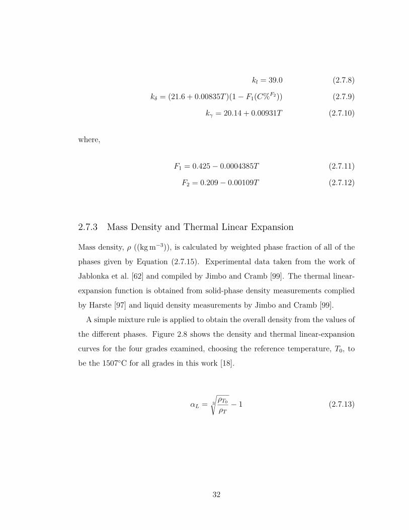
2.7.3 Mass Density and Thermal Linear Expansion

Mass density, ρ ((kg m−3)), is calculated by weighted phase fraction of all of the

phases given by Equation (2.7.15). Experimental data taken from the work of

Jablonka et al. [62] and compiled by Jimbo and Cramb [99]. The thermal linear-

expansion function is obtained from solid-phase density measurements complied

by Harste [97] and liquid density measurements by Jimbo and Cramb [99].

A simple mixture rule is applied to obtain the overall density from the values of

the different phases. Figure 2.8 shows the density and thermal linear-expansion

curves for the four grades examined, choosing the reference temperature, T0, to

be the 1507◦C for all grades in this work [18].

αL = 3

√ρT0

ρT− 1 (2.7.13)

32

28

30

32

34

36

38

40

Ther

mal

Con

duct

ivity

[W/m

2 K]

Ultra-Low Carbon (0.003 %)Low Carbon (0.03 %)Peritectic (0.13 %)High Carbon (0.47 %)

1300 1400 1500 1600 1700 1800Temperature [K]

700

800

900

1000

1100

1200

1300

1400

1500

Ent

halp

y[k

J/kg

]

Ultra-Low Carbon (0.003 %)Low Carbon (0.03 %)Peritectic (0.13 %)High Carbon (0.47 %)

7000

7100

7200

7300

7400

7500

7600

7700

Den

sity

[kg/

m3 ]

Ultra-Low Carbon (0.003 %)Low Carbon (0.03 %)Peritectic (0.13 %)High Carbon (0.47 %)

1000 1100 1200 1300 1400 1500 1600Temperature [◦C]

0.000

0.005

0.010

0.015

0.020

TLE

[%]

Ultra-Low Carbon (0.003 %)Low Carbon (0.03 %)Peritectic (0.13 %)High Carbon (0.47 %)

Figure 2.8: Temperature-dependent properties of four steel grades investigated:a) Thermal conductivity b) Enthalpy c)Density d) Thermal linear expansion

33

ρl = 7100− 73.2CC − (0.828− 0.0874CC)(T − 1550) (2.7.14a)

ρδ = 100(8011− 0.47T )(100− CC)(1 + 0.013CC)3 (2.7.14b)

ργ = 100(8106− 0.51T )(100− CC)(1 + 0.008CC)3 (2.7.14c)

ρα = 7881− 0.324T − 3× 10−5T 2 (2.7.14d)

ρT [kg m−3] = ρlfl + ρδfδ + ργfγ + ραfα (2.7.15)

Where αL is the Thermal Linear Expansion coefficient and the density ρT0 is

the density at the reference temperature T0. For this work ρT0 is taken to be 7400

kg m−3 .

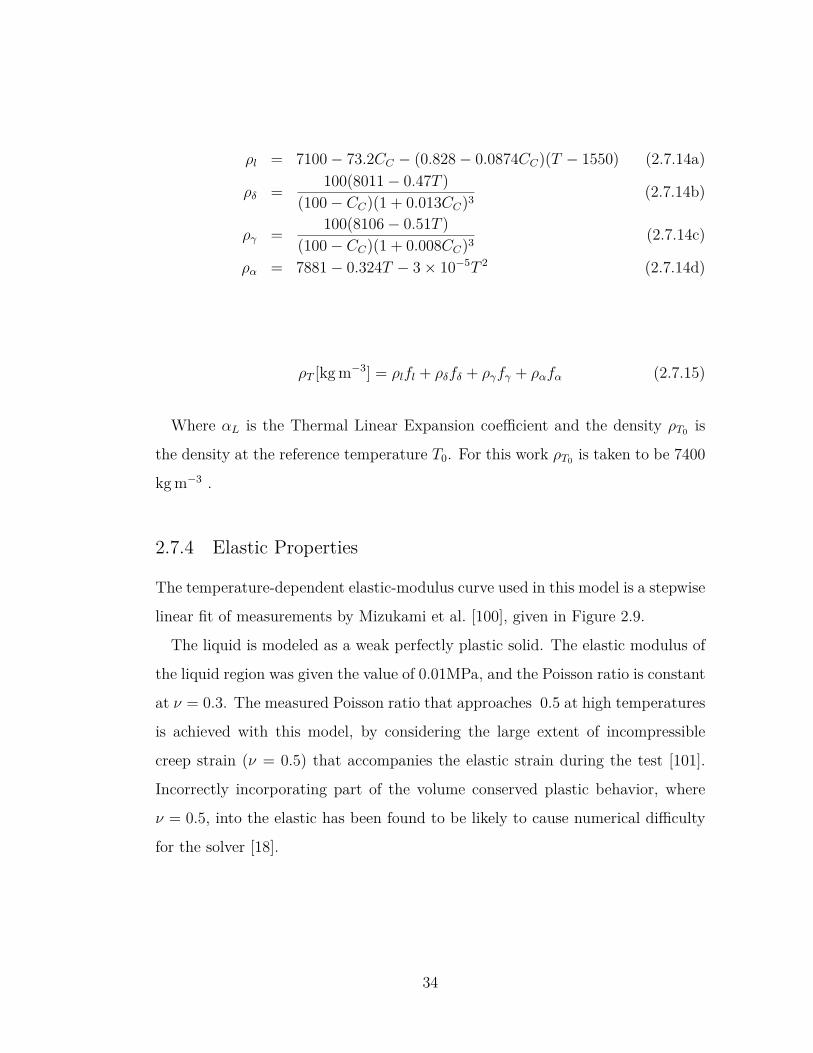
2.7.4 Elastic Properties

The temperature-dependent elastic-modulus curve used in this model is a stepwise

linear fit of measurements by Mizukami et al. [100], given in Figure 2.9.

The liquid is modeled as a weak perfectly plastic solid. The elastic modulus of

the liquid region was given the value of 0.01MPa, and the Poisson ratio is constant

at ν = 0.3. The measured Poisson ratio that approaches 0.5 at high temperatures

is achieved with this model, by considering the large extent of incompressible

creep strain (ν = 0.5) that accompanies the elastic strain during the test [101].

Incorrectly incorporating part of the volume conserved plastic behavior, where

ν = 0.5, into the elastic has been found to be likely to cause numerical difficulty

for the solver [18].

34

Figure 2.9: Temperature-dependent elastic modulus of steel

2.7.5 Constitutive Models

Two constitutive models relating the stress-strain relationship are utilized in this

work. These equations were developed to match tensile-test measurements of

Wray [102] and creep-test data of Suzuki et al [47]. The details of these two

models can be found in [103] and [104] respectively.

The ferrite and austenite phases are not of comparable strength. Ferrite is

approximately an order of magnitude weaker than austenite of the same temper-

ature, because of this a weighted mixture rule is not appropriate in regions with

the much weaker phase when the softer material dominates the net mechanical

behavior. In previous works where these two constitutive equations were utilized,

Equation (2.7.17) was in effect when there was less than 10% of either ferrite

phase, otherwise Equation (2.7.16) was used. This work also uses this method.

Improving upon this transition method is left for future work.

Two different constitutive equations are used to model the behavior of solidify-

ing steel. Equation (2.7.16) is the Zhu Modified Power law [103] and is used for

35

ferrite.

ε̇in−δ[1/s] = 0.1Fδ|Fδ|n−1 (2.7.16)

where,

Fδ = Cσ

fC(T (K)300 )−5.52(1 + 1000|εin|)m

fC = 1.3678× 104C−5.56×10−2

C

m = −9.4156× 10−5T (K) + 0.349501

n = (1.617× 10−4T (K)− 0.06166)−1

C represents the sign on the 3 dimensional stress tensor [105], and CC is the

wt.% carbon.

Equation Equation (2.7.17) is the Kozlowski model III [104] which is used for

austenite.

ε̇in−γ[1/s] = fC |Fγ|f3−1Fγexp(−4.465× 104

T (K) ) (2.7.17)

where,

Fγ = Cσ − f1εin|εin|f2−1

f1 = 130.5− 5.128× 10−3T (K)

f2 = −0.6289 + 1.114× 10−3T (K)

f3 = 8.132− 1.54× 10−3T (K)

fC = 4.655× 104 + 7.14× 104CC + 1.2× 105C2C

36

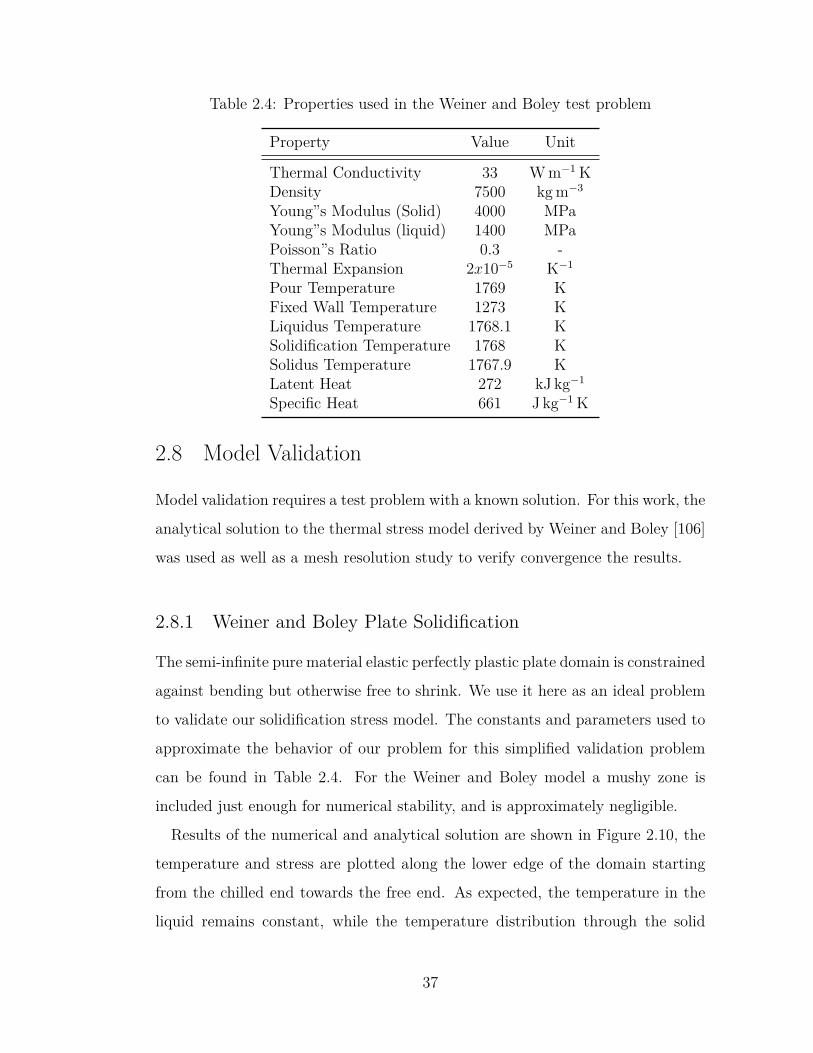
Table 2.4: Properties used in the Weiner and Boley test problem

Property Value Unit

Thermal Conductivity 33 W m−1 KDensity 7500 kg m−3

Young”s Modulus (Solid) 4000 MPaYoung”s Modulus (liquid) 1400 MPaPoisson”s Ratio 0.3 -Thermal Expansion 2x10−5 K−1

Pour Temperature 1769 KFixed Wall Temperature 1273 KLiquidus Temperature 1768.1 KSolidification Temperature 1768 KSolidus Temperature 1767.9 KLatent Heat 272 kJ kg−1

Specific Heat 661 J kg−1 K

2.8 Model Validation

Model validation requires a test problem with a known solution. For this work, the

analytical solution to the thermal stress model derived by Weiner and Boley [106]

was used as well as a mesh resolution study to verify convergence the results.

2.8.1 Weiner and Boley Plate Solidification

The semi-infinite pure material elastic perfectly plastic plate domain is constrained

against bending but otherwise free to shrink. We use it here as an ideal problem

to validate our solidification stress model. The constants and parameters used to

approximate the behavior of our problem for this simplified validation problem

can be found in Table 2.4. For the Weiner and Boley model a mushy zone is

included just enough for numerical stability, and is approximately negligible.

Results of the numerical and analytical solution are shown in Figure 2.10, the

temperature and stress are plotted along the lower edge of the domain starting

from the chilled end towards the free end. As expected, the temperature in the

liquid remains constant, while the temperature distribution through the solid

37

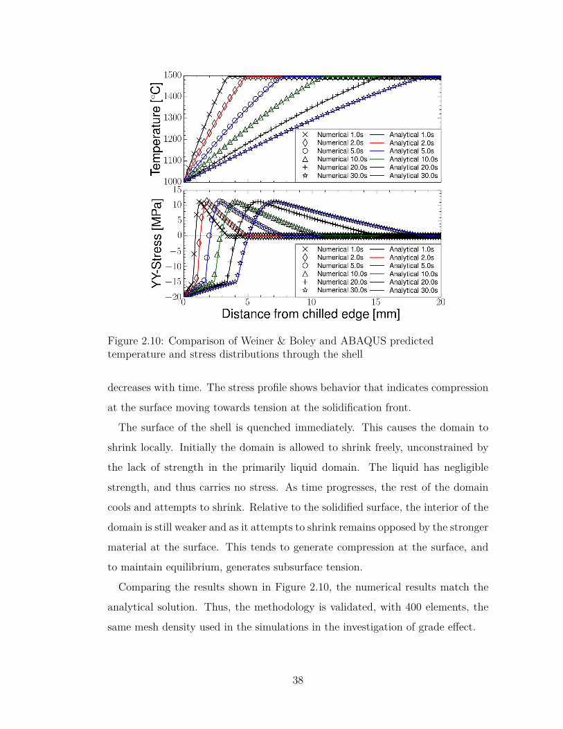
Figure 2.10: Comparison of Weiner & Boley and ABAQUS predictedtemperature and stress distributions through the shell

decreases with time. The stress profile shows behavior that indicates compression

at the surface moving towards tension at the solidification front.

The surface of the shell is quenched immediately. This causes the domain to

shrink locally. Initially the domain is allowed to shrink freely, unconstrained by

the lack of strength in the primarily liquid domain. The liquid has negligible

strength, and thus carries no stress. As time progresses, the rest of the domain

cools and attempts to shrink. Relative to the solidified surface, the interior of the

domain is still weaker and as it attempts to shrink remains opposed by the stronger

material at the surface. This tends to generate compression at the surface, and

to maintain equilibrium, generates subsurface tension.

Comparing the results shown in Figure 2.10, the numerical results match the

analytical solution. Thus, the methodology is validated, with 400 elements, the

same mesh density used in the simulations in the investigation of grade effect.

38

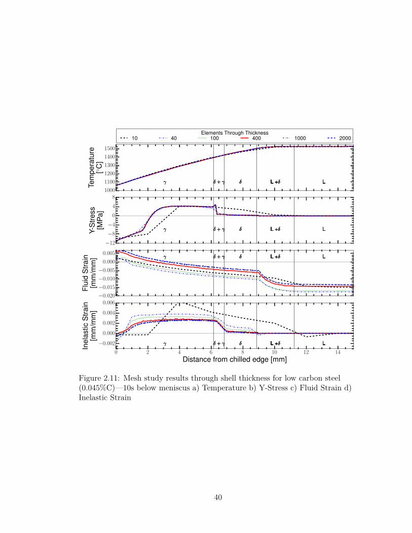
2.8.2 Mesh Resolution

A mesh study was conducted to verify that the model was converging to a proper

solution, changing only the number of elements through the solidification direction

(x). The domain width was chosen to maintain 3 elements through the thickness

and an aspect ratio of 1. (i.e. the 10-elements case has 4mm square elements,

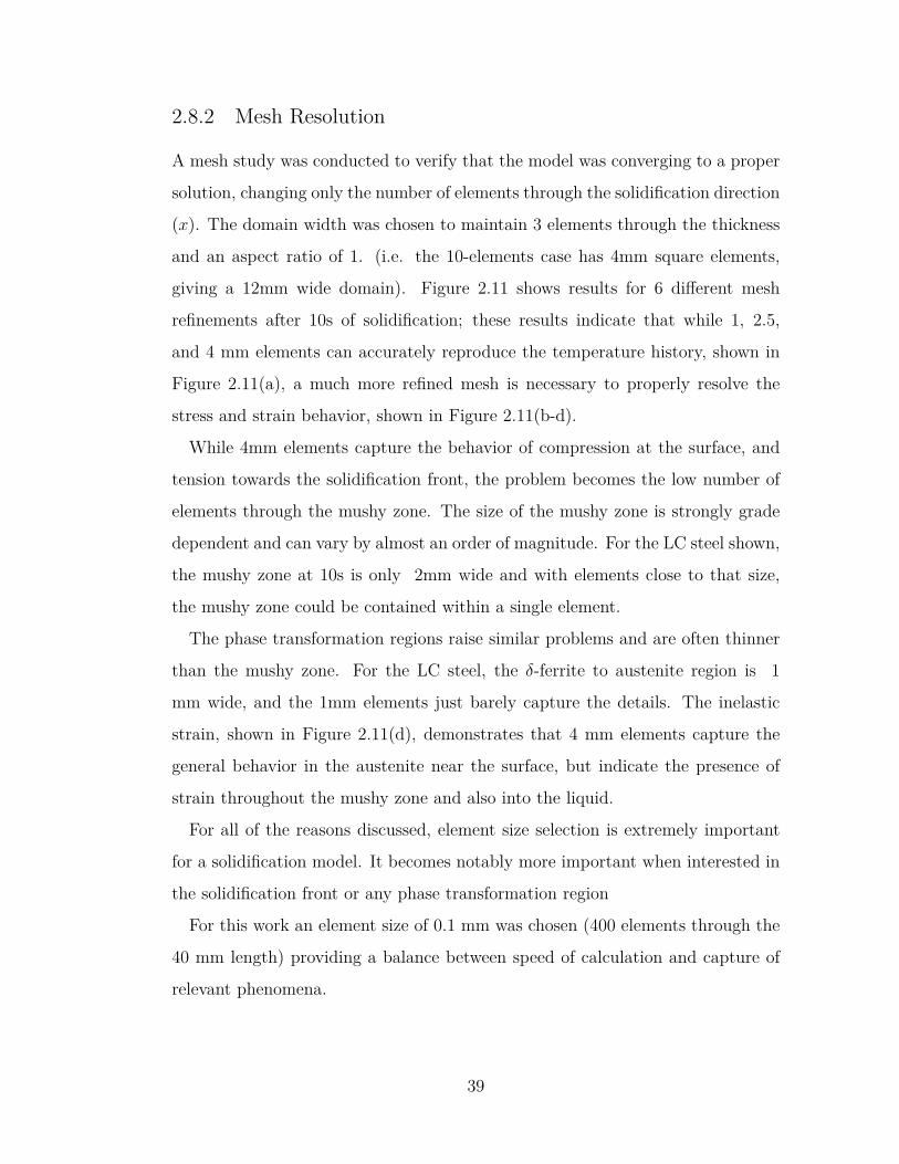
giving a 12mm wide domain). Figure 2.11 shows results for 6 different mesh

refinements after 10s of solidification; these results indicate that while 1, 2.5,

and 4 mm elements can accurately reproduce the temperature history, shown in

Figure 2.11(a), a much more refined mesh is necessary to properly resolve the

stress and strain behavior, shown in Figure 2.11(b-d).

While 4mm elements capture the behavior of compression at the surface, and

tension towards the solidification front, the problem becomes the low number of

elements through the mushy zone. The size of the mushy zone is strongly grade

dependent and can vary by almost an order of magnitude. For the LC steel shown,

the mushy zone at 10s is only 2mm wide and with elements close to that size,

the mushy zone could be contained within a single element.

The phase transformation regions raise similar problems and are often thinner

than the mushy zone. For the LC steel, the δ-ferrite to austenite region is 1

mm wide, and the 1mm elements just barely capture the details. The inelastic

strain, shown in Figure 2.11(d), demonstrates that 4 mm elements capture the

general behavior in the austenite near the surface, but indicate the presence of

strain throughout the mushy zone and also into the liquid.

For all of the reasons discussed, element size selection is extremely important

for a solidification model. It becomes notably more important when interested in

the solidification front or any phase transformation region

For this work an element size of 0.1 mm was chosen (400 elements through the

40 mm length) providing a balance between speed of calculation and capture of

relevant phenomena.

39

1000

1100

1200

1300

1400

1500

Tem

pera

ture

[◦C

]

γ δ + γ δ L +δ Lγ δ + γ δ L +δ Lγ δ + γ δ L +δ Lγ δ + γ δ L +δ L

Elements Through Thickness10 40 100 400 1000 2000

−12

−8

−4

0

4

8

Y-S

tress

[MP

a]

γ δ + γ δ L +δ Lγ δ + γ δ L +δ Lγ δ + γ δ L +δ Lγ δ + γ δ L +δ L

−0.020

−0.015

−0.010

−0.005

0.000

0.005

Flui

dS

train

[mm

/mm

] γ δ + γ δ L +δ Lγ δ + γ δ L +δ Lγ δ + γ δ L +δ Lγ δ + γ δ L +δ L

0 2 4 6 8 10 12 14

Distance from chilled edge [mm]

−0.002

0.000

0.002

0.004

0.006

Inel

astic

Stra

in[m

m/m

m]

γ δ + γ δ L +δ Lγ δ + γ δ L +δ Lγ δ + γ δ L +δ Lγ δ + γ δ L +δ L

Figure 2.11: Mesh study results through shell thickness for low carbon steel(0.045%C)—10s below meniscus a) Temperature b) Y-Stress c) Fluid Strain d)Inelastic Strain

40

2.9 Solution Method & Details

The governing equations are solved incrementally using the finite-element method

[107] in ABAQUS/Standard [108] (implicit). Analysis was performed in two sepa-

rate steps consisting of the 30s heat transfer analysis, followed by the 30s mechan-

ical analysis, with the heat transfer solution as input for each time increment of

the mechanical step. While this neglects the nonlinear coupling between the me-

chanical and thermal solutions, the “one-way coupled” method, has been shown to

be reasonable in regions of uniform heat transfer [109] and is appropriate for our

simplified case. Details of the numerical method are provided elsewhere [64,105].

DCC2D4 4-node linear diffusive heat transfer elements were used for the thermal

problem and CPEG4H 4-node bilinear quadrilateral elements for the stress. The

time step size was allowed to vary from 0.00001s to 1s, controlled by ABAQUS,

with a maximum temperature change per increment of 10◦C. Output was re-

quested at 0.05s intervals. Each grade simulation required about one hr wall-clock

time on one core of a Dell Precision T7600 workstation with 2 Intel Xeon 1.8GHz

quad-core processors and 64GB of DDR3 SDRAM. The Peritectic and Ultra-Low

Carbon grades took slightly longer than the others due to the abrupt changes in

phase fraction visible in Figure 2.6

2.10 Results and Discussion

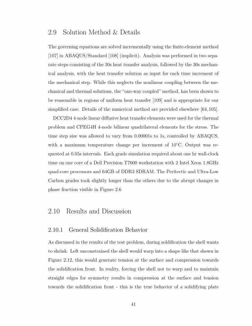
2.10.1 General Solidification Behavior

As discussed in the results of the test problem, during soldification the shell wants

to shrink. Left unconstrained the shell would warp into a shape like that shown in

Figure 2.12, this would generate tension at the surface and compression towards

the solidification front. In reality, forcing the shell not to warp and to maintain

straight edges for symmetry results in compression at the surface and tension

towards the solidification front - this is the true behavior of a solidifying plate

41

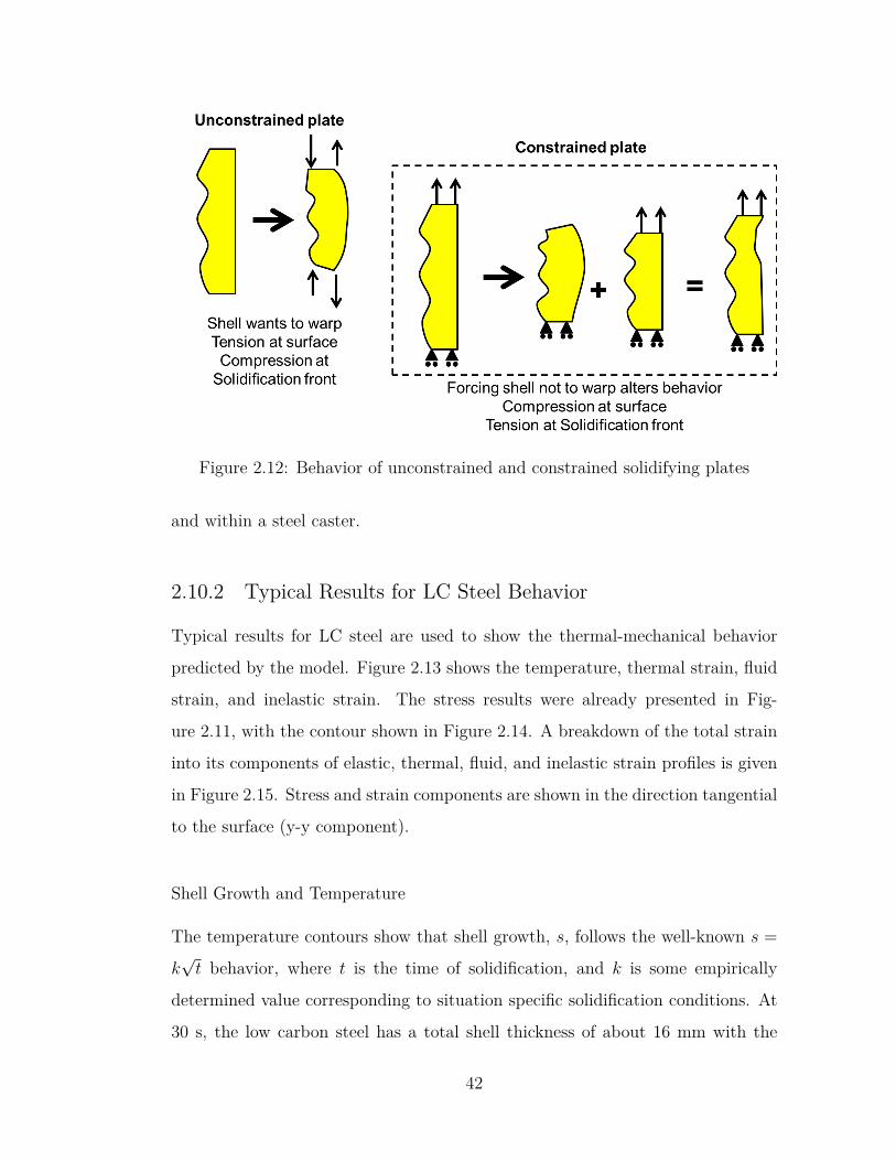
Figure 2.12: Behavior of unconstrained and constrained solidifying plates

and within a steel caster.

2.10.2 Typical Results for LC Steel Behavior

Typical results for LC steel are used to show the thermal-mechanical behavior

predicted by the model. Figure 2.13 shows the temperature, thermal strain, fluid

strain, and inelastic strain. The stress results were already presented in Fig-

ure 2.11, with the contour shown in Figure 2.14. A breakdown of the total strain

into its components of elastic, thermal, fluid, and inelastic strain profiles is given

in Figure 2.15. Stress and strain components are shown in the direction tangential

to the surface (y-y component).

Shell Growth and Temperature

The temperature contours show that shell growth, s, follows the well-known s =

k√t behavior, where t is the time of solidification, and k is some empirically

determined value corresponding to situation specific solidification conditions. At

30 s, the low carbon steel has a total shell thickness of about 16 mm with the

42

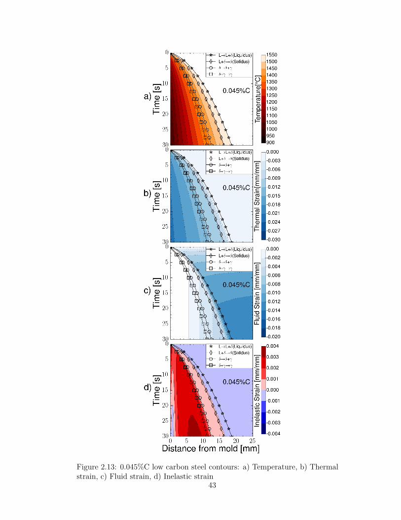
Figure 2.13: 0.045%C low carbon steel contours: a) Temperature, b) Thermalstrain, c) Fluid strain, d) Inelastic strain

43

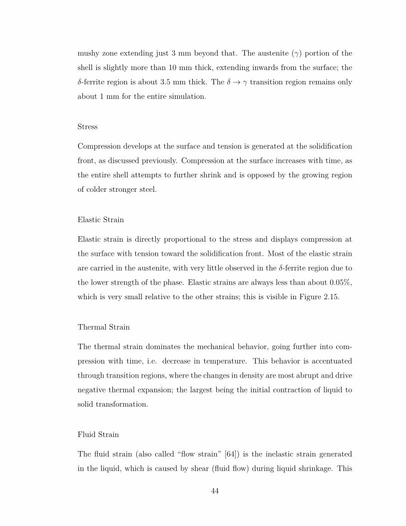
mushy zone extending just 3 mm beyond that. The austenite (γ) portion of the

shell is slightly more than 10 mm thick, extending inwards from the surface; the

δ-ferrite region is about 3.5 mm thick. The δ → γ transition region remains only

about 1 mm for the entire simulation.

Stress

Compression develops at the surface and tension is generated at the solidification

front, as discussed previously. Compression at the surface increases with time, as

the entire shell attempts to further shrink and is opposed by the growing region

of colder stronger steel.

Elastic Strain

Elastic strain is directly proportional to the stress and displays compression at

the surface with tension toward the solidification front. Most of the elastic strain

are carried in the austenite, with very little observed in the δ-ferrite region due to

the lower strength of the phase. Elastic strains are always less than about 0.05%,

which is very small relative to the other strains; this is visible in Figure 2.15.

Thermal Strain

The thermal strain dominates the mechanical behavior, going further into com-

pression with time, i.e. decrease in temperature. This behavior is accentuated

through transition regions, where the changes in density are most abrupt and drive

negative thermal expansion; the largest being the initial contraction of liquid to

solid transformation.

Fluid Strain

The fluid strain (also called “flow strain” [64]) is the inelastic strain generated

in the liquid, which is caused by shear (fluid flow) during liquid shrinkage. This

44

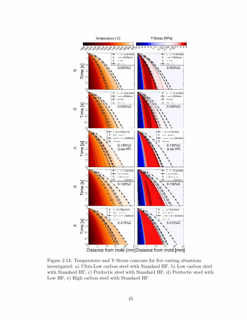
Figure 2.14: Temperature and Y-Stress contours for five casting situationsinvestigated: a) Ultra-Low carbon steel with Standard HF, b) Low carbon steelwith Standard HF, c) Peritectic steel with Standard HF, d) Peritectic steel withLow HF, e) High carbon steel with Standard HF

45

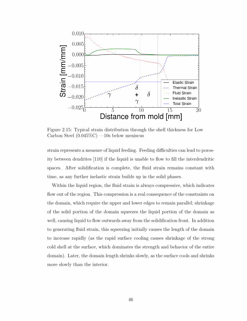
Figure 2.15: Typical strain distribution through the shell thickness for LowCarbon Steel (0.045%C) —10s below meniscus

strain represents a measure of liquid feeding. Feeding difficulties can lead to poros-

ity between dendrites [110] if the liquid is unable to flow to fill the interdendritic

spaces. After solidification is complete, the fluid strain remains constant with

time, as any further inelastic strain builds up in the solid phases.

Within the liquid region, the fluid strain is always compressive, which indicates

flow out of the region. This compression is a real consequence of the constraints on

the domain, which require the upper and lower edges to remain parallel; shrinkage

of the solid portion of the domain squeezes the liquid portion of the domain as

well, causing liquid to flow outwards away from the solidification front. In addition

to generating fluid strain, this squeezing initially causes the length of the domain

to increase rapidly (as the rapid surface cooling causes shrinkage of the strong

cold shell at the surface, which dominates the strength and behavior of the entire

domain). Later, the domain length shrinks slowly, as the surface cools and shrinks

more slowly than the interior.

46

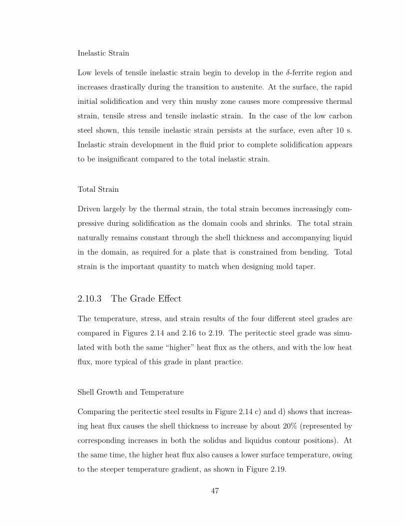
Inelastic Strain

Low levels of tensile inelastic strain begin to develop in the δ-ferrite region and

increases drastically during the transition to austenite. At the surface, the rapid

initial solidification and very thin mushy zone causes more compressive thermal

strain, tensile stress and tensile inelastic strain. In the case of the low carbon

steel shown, this tensile inelastic strain persists at the surface, even after 10 s.

Inelastic strain development in the fluid prior to complete solidification appears

to be insignificant compared to the total inelastic strain.

Total Strain

Driven largely by the thermal strain, the total strain becomes increasingly com-

pressive during solidification as the domain cools and shrinks. The total strain

naturally remains constant through the shell thickness and accompanying liquid

in the domain, as required for a plate that is constrained from bending. Total

strain is the important quantity to match when designing mold taper.

2.10.3 The Grade Effect

The temperature, stress, and strain results of the four different steel grades are

compared in Figures 2.14 and 2.16 to 2.19. The peritectic steel grade was simu-

lated with both the same “higher” heat flux as the others, and with the low heat

flux, more typical of this grade in plant practice.

Shell Growth and Temperature

Comparing the peritectic steel results in Figure 2.14 c) and d) shows that increas-

ing heat flux causes the shell thickness to increase by about 20% (represented by

corresponding increases in both the solidus and liquidus contour positions). At

the same time, the higher heat flux also causes a lower surface temperature, owing

to the steeper temperature gradient, as shown in Figure 2.19.

47

Increasing carbon content causes increased thickness of the mushy zone, ac-

cording to the increasing temperature range between the liquidus and solidus

temperatures, as shown in the left side of Figure 2.14. With the same superheat,

the liquid temperature decreases with increasing carbon content, as shown in the

top right of Figure 2.19, so the temperature profiles of the four grades become

correspondingly lower.

The effect of steel grade on shell thickness is complicated, because it depends

on the thermal properties, the heat flux, and the definition of shell thickness.

Except for the peritectic steel, increasing the carbon content increases the liquidus

thickness and decreases the solidus thickness, due to the increase in mushy zone

thickness.

Stress

For all four steels, the general stress profile of compression at the surface increas-

ing to tension near the solidification and down to zero in the liquid, as shown in

Figure 2.18. At early times in ULC and LC steels, however, a brief tensile peak

appears at the surface, due to the rapid cooling and shrinkage, as shown in Fig-

ure 2.18(b). This generates a corresponding very mild compression region inside

the δ-ferrite for a brief period, which can be seen in the top left of Figure 15 (a-b)

stress frames. As time increases beyond 2 s, surface stress becomes compressive

in all steel grades. As the steel continues to cool and strengthen, the magnitude

of this surface compression increases. For the same reason, decreasing the heat

flux (in the peritectic steel) causes higher temperatures and lower absolute stress

levels, both at the surface and in the interior.

Figure 2.14 shows low stress in the δ-ferrite whenever that phase appears, which

is due to its low strength and inability to carry any significant load. Moving

towards the left, a sharp increase in strength from δ-ferrite to austenite is observed,

which is accompanied by a pointed peak. Although this peak is not a numerical

error, it is an artifact that disappears when the phase transition occurs over a

48

wide temperature range. Naturally, this peak is missing from high carbon steel,

which has no delta phase, so its stress transition is smooth across the austenite

near the solidification front.

The sharp increase in strength from δ-ferrite to austenite causes a pointed peak

to appear in the stress profile. Although this peak is not a numerical error, it is

an artifact that disappears when the phase transition occurs over a temperature

range. Naturally, this peak is missing from high carbon steel, which has no δ

phase, so the stress peak is smooth.

Strain Results

Contours of the thermal, fluid, and inelastic strain components are compared for

the four steels in Figure 2.16. The dominant component, thermal strain, increases

in magnitude as temperature decreases. Thus, the greatest magnitude thermal

strain is found at the surface, where it increases with decreasing carbon content.

The fluid strain evolution in all grades is similar to that discussed for LC steel

previously. Fluid strain is always negative, indicating shrinkage. The greatest

magnitude fluid strain is observed in the peritectic steel at standard heat flux,

owing to the greater shrinkage of this grade for the higher heat flux.

The inelastic strain results in Figure 2.17 show that the initial tensile inelastic

strain peak decreases in magnitude with increasing carbon content. This increased

tensile peak results in the lower-carbon steel grades (below 0.13 %C) remaining in

tension at the surface, even after 30 s when the higher carbon grades have become

compressive, this agrees with previous results [111]. This persistent tension is

likely caused by the rapid shrinkage as a result of the narrow mushy zone in both

the ULC and LC steels.

49

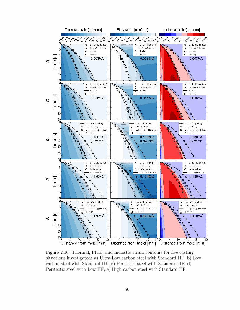
Figure 2.16: Thermal, Fluid, and Inelastic strain contours for five castingsituations investigated: a) Ultra-Low carbon steel with Standard HF, b) Lowcarbon steel with Standard HF, c) Peritectic steel with Standard HF, d)Peritectic steel with Low HF, e) High carbon steel with Standard HF

50

Elastic The elastic strain is seen to peak at the austenite repacking transition

of BCC to FCC. The transition manifests itself with an abrupt increase in Elastic

strain at the 10%δ-90%austenite temp (corresponding an increase in strength of

the region when it transforms from δ-BCC to austenite-FCC), followed directly

by a drop to almost a strain-less condition ending with a slight increase back to

positive strain at only a fraction of its previous (BCC) strain. It appears that

high carbon steels have slightly lower elastic strain before this transition peak

than the other grades, additionally it would seem that the Ultra-low carbon steel

exhibits the highest relative elastic strain before and after this transition.

Inelastic Strain It can be observed that in all steel grades there is an initial

period with development of negative inelastic strain. This effect becomes more

apparent in the higher carbon content steels. This development occurs only within

the δ-ferrite phase and quickly dissipates after 3 seconds. As we near the end of

the simulation we observe that the inelastic strain at the surface has continued

to decrease from its initial values, however, while the P, LC, and ULC appear to

become negative the high carbon remains positive. It was observed however that

qualitatively they are all moving in the negative direction.

2.10.4 Taper Practices

Strand solidification during continuous casting results in a shrinking cross-section

down the caster. To accommodate this shrinkage and maintain support of the

shell, a taper is applied to the mold on both the wide and narrow face coppers.

Linear taper practices apply a fixed angle to the flat narrow face mold copper.

While taper (and width) changes are sometimes conducted during casting, applied

taper for a given heat is decided apriori based on the casting conditions and the

grade being cast.

As mentioned before, differences in taper from the ideal shrinkage of the strand

(under or over taper) can results in a variety of quality problems, for these reasons

51

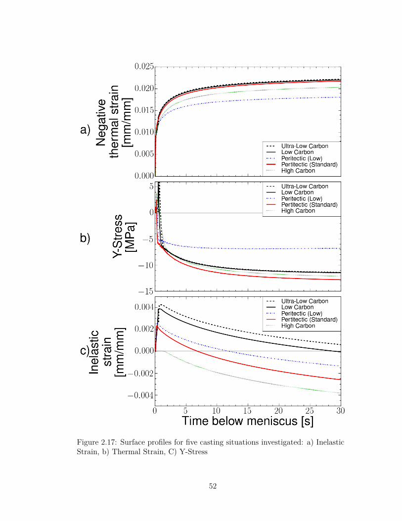
Figure 2.17: Surface profiles for five casting situations investigated: a) InelasticStrain, b) Thermal Strain, C) Y-Stress

52

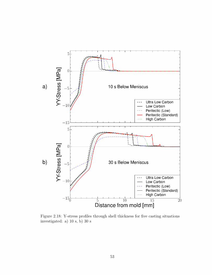
Figure 2.18: Y-stress profiles through shell thickness for five casting situationsinvestigated: a) 10 s, b) 30 s

53

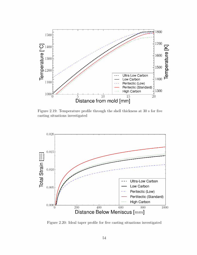
Figure 2.19: Temperature profile through the shell thickness at 30 s for fivecasting situations investigated

Figure 2.20: Ideal taper profile for five casting situations investigated

54

it is important the applied taper is closest to the ideal shrinkage for a given grade

and casting condition. As shown in Figure 2.20 the ideal shrinkage profile for

all of the steel grades is parabolic. The large initial shrinkage is a result of the

sudden change in density as the crystal structure transitions from BCC to FCC.

The majority of the shell shrinkage occurs during this transition period, after

this this point the shell continues to shrink but the change is much smaller in

magnitude.

While ferrostatic pressure aids in maintaining surface contact between the so-

lidifying shell and the narrow face copper, applying a linear taper profile to an

ideally parabolic shrinkage profile is likely to result in under taper, allow a gap

to form, and potential bulging of the shell.

The peritectic grade simulated with both Low and Standard HF demonstrate

that cooling rate has a strong effect on the final taper, increasing total strain by

almost 50% with increased HF.

The ideal shrinkage profiles presented give a good starting point for general

understanding of taper trends; however it does not provide all of the information

required for proper taper selection.

In an operating caster mold distortion affects the operating shape of the copper.

In a distorted mold, thermal expansion tends to cause the narrow face coppers to

try and bow in towards the strand center-line. This results in a different realized

taper than what is applied or indicated by sensors such as inclinometers. De-

pending on the water box support and bolt pattern, this can cause unpredictable

results including premature mold wear and non-uniform changes in taper down

the caster. Detailed discussion of mold distortion can be found elsewhere [112]

Taper based on TLE

Prior works have suggested that a basic taper practice should begin by looking at

the expected TLE profile for a given grade. While this is a good starting point,

it does generally result in an overestimation of the total shrinkage of the strand.

55

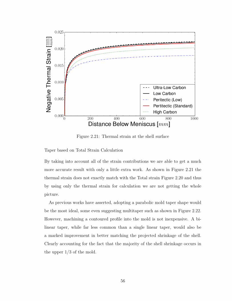
Figure 2.21: Thermal strain at the shell surface

Taper based on Total Strain Calculation

By taking into account all of the strain contributions we are able to get a much

more accurate result with only a little extra work. As shown in Figure 2.21 the

thermal strain does not exactly match with the Total strain Figure 2.20 and thus

by using only the thermal strain for calculation we are not getting the whole

picture.

As previous works have asserted, adopting a parabolic mold taper shape would

be the most ideal, some even suggesting multitaper such as shown in Figure 2.22.

However, machining a contoured profile into the mold is not inexpensive. A bi-

linear taper, while far less common than a single linear taper, would also be

a marked improvement in better matching the projected shrinkage of the shell.

Clearly accounting for the fact that the majority of the shell shrinkage occurs in

the upper 1/3 of the mold.

56

Grade Based Taper Practice

The results of this work have implications for optimal taper practice. Solidifi-

cation and cooling result in shrinking of the steel shell; this shrinkage should

be accommodated in order to maintain contact between the edges of the shell

and the mold walls without an excessive air gap. This is accomplished in con-

tinuous casting by applying a taper to the mold walls that roughly matches this

shrinkage represented by the total strain. Proper taper practice is important to

mold operation to ensure safe, uniform heat transfer between the mold and shell,

and to reduce the likelihood of surface defects and breakouts. Insufficient taper

causes insufficient and non-uniform heat transfer between the strand and the mold

across the gap, which can lead to corner rotation, shell thinning, and narrow face

bulging [113]. Excessive taper can lead to many problems such as excessive mold

wear, gutter, or even buckling of the shell. Both taper problems can cause gutter,

longitudinal cracks, and breakouts.

As shown in Figure 2.20 the ideal taper profile for all of the steel grades is

parabolic, according to total shrinkage, which is indicated by the total y-y strain

decreasing with time down the mold. This shrinkage is controlled mainly by

the drop in surface temperature, because the shell at the surface is coldest and

strongest. The majority of the shell shrinkage occurs during this transition period

while the shell is about 5 mm thick. After this this point the shell continues to

shrink but the change is much smaller in magnitude as it is opposed by the

increasing thickness and strength of the shell.

For the same heat flux, the peritectic steel experiences the greatest shrinkage

and ideal taper, while the other three steels have similar, but lower profiles. This

is because the large shrinkage that accompanies the δ-ferrite to austenite phase

transformation occurs in the solid at high temperature in the peritectic steel, while

the shell is still hot and weak, and unable to resist the shrinkage. However, with

decreased heat flux, that is typical of the real commercial process, the peritectic

steel experiences about 30% less shrinkage and ideal taper. The great dependence

57

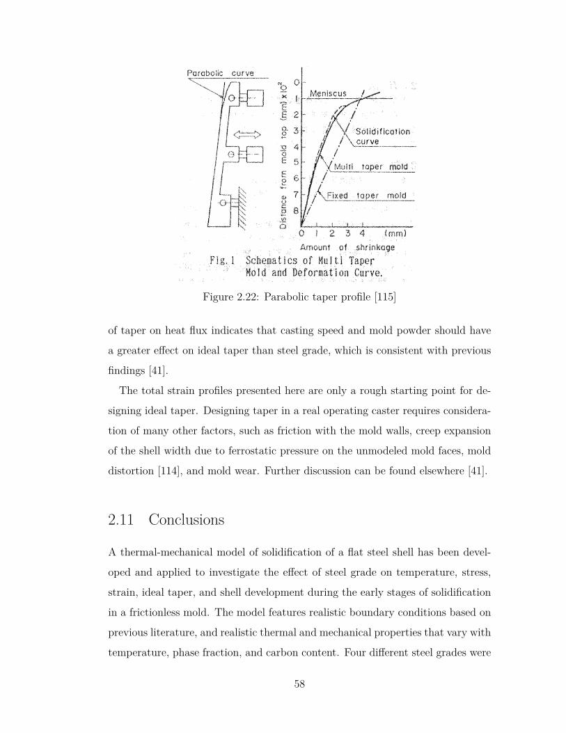
Figure 2.22: Parabolic taper profile [115]

of taper on heat flux indicates that casting speed and mold powder should have

a greater effect on ideal taper than steel grade, which is consistent with previous

findings [41].

The total strain profiles presented here are only a rough starting point for de-

signing ideal taper. Designing taper in a real operating caster requires considera-

tion of many other factors, such as friction with the mold walls, creep expansion

of the shell width due to ferrostatic pressure on the unmodeled mold faces, mold

distortion [114], and mold wear. Further discussion can be found elsewhere [41].

2.11 Conclusions

A thermal-mechanical model of solidification of a flat steel shell has been devel-

oped and applied to investigate the effect of steel grade on temperature, stress,

strain, ideal taper, and shell development during the early stages of solidification

in a frictionless mold. The model features realistic boundary conditions based on

previous literature, and realistic thermal and mechanical properties that vary with

temperature, phase fraction, and carbon content. Four different steel grades were

58

investigated: Ultra-Low Carbon (0.003 %C), Low Carbon (0.04 %C), Peritectic

(0.13 %C), and High Carbon (0.47 %C), simulating 30 s dwell times.

Mesh refinement for capturing solidification details was examined and element

sizes of 0.1 mm or smaller may be required to properly study solidification phenom-

ena. Proper treatment of the liquid in the stress model can alleviate convergence

problems and avoid non-physical results.

• All steel grades were found to follow the same general solidification behavior

of compression at the surface increasing with time, and tension towards the

solidification front

• Initial solidification rate increases with carbon content

• Thermal strain dominates the mechanical behavior. Initially, fast cooling

causes tensile stress and inelastic strain at the surface of the shell, with

slight complementary compression beneath the surface, especially with lower

carbon content

• As the cooling rate decreases, the surface then reverses into compression,

with a tensile region developing subsurface . Stress decreases towards zero

(the ferrostatic pressure) at the solidification front.

• More stress and inelastic strain are generated in the high carbon steels,

because they are mainly composed of high-strength austenite

• Stress in the δ-ferrite phase is always very small, owing to the low strength

of this phase

This simple model can help in the calculation of taper profiles for different steel

grades and maintain the desired contact. While fixed linear taper practices are

common in industry, it is clear that the desired profile of the shell is parabolic,

which agrees with previous work [115].

59

2.12 Future Work

This work is the first step in development, validation, and application of a com-

prehensive transient 3-D model of thermal-mechanical behavior during continuous

casting of steel slabs, including corner effects and non-uniform heat flux around

the mold perimeter. In this modeling approach, the properties of different steel

grades depend mainly on the phase fraction histories. This enables predictions of

any steel grade knowing only the phase fraction histories, so extensive experimen-

tal testing is not required. Validation of this approach with measurements would

be helpful, and is intended as future work.

60

Chapter 3

Thermal Resistor Model of the Shell-Mold Gap

3.1 Introduction

In continuous casting, as the liquid steel solidifies against the four walls of the

water-cooled copper mold, the solidifying shell ideally does not come into direct

contact with the mold copper. Mold powder is added to the free surface of the

liquid steel, melts and flows between the steel shell and the mold wall to act

as a lubricant. The re-solidified mold powder, or ’slag’, adjacent to the mold

wall cools and greatly increases in viscosity, thus acting like a solid. It is thicker

near and just above the meniscus, where it is called the ’slag rim’. Depending on

temperature, cooling rate, and cooling history, this slag layer may have a structure

that is glassy, crystalline, or a combination as shown in Figure 3.1. As long as the

interface temperature remains above its crystallization temperature, the slag layer

will remain liquid and provide lubrication for the shell as it moves downward. If

the interface temperature is at or below the crystallization temperature, liquid

and solid layers may be present, and if the conditions allow, an air gap may form

within the gap.

As the shell travels down the mold and solidifies it shrinks due to phase changes

and thermal contraction. If the taper calculation is not adequate, an air gap may

form in the space between the shell and the mold. The gap may also be affected

by mold distortion warping the copper out of it’s expected shape. The size of

the gap is particularly important when exploring positions near the corner where

geometry effects and shell strength outweigh ferrostatic pressure.

It has been estimated that the gap alone accounts for as much as 84% of the

61

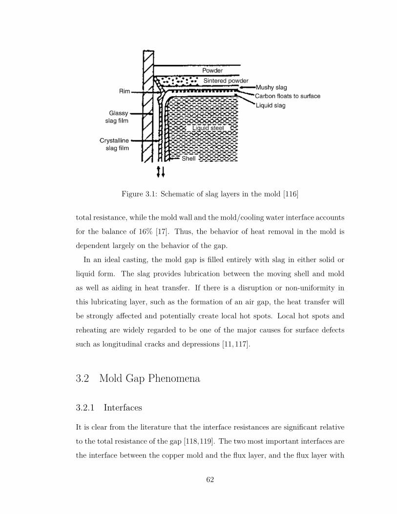
Figure 3.1: Schematic of slag layers in the mold [116]

total resistance, while the mold wall and the mold/cooling water interface accounts

for the balance of 16% [17]. Thus, the behavior of heat removal in the mold is

dependent largely on the behavior of the gap.

In an ideal casting, the mold gap is filled entirely with slag in either solid or

liquid form. The slag provides lubrication between the moving shell and mold

as well as aiding in heat transfer. If there is a disruption or non-uniformity in

this lubricating layer, such as the formation of an air gap, the heat transfer will

be strongly affected and potentially create local hot spots. Local hot spots and

reheating are widely regarded to be one of the major causes for surface defects

such as longitudinal cracks and depressions [11,117].

3.2 Mold Gap Phenomena

3.2.1 Interfaces

It is clear from the literature that the interface resistances are significant relative

to the total resistance of the gap [118,119]. The two most important interfaces are

the interface between the copper mold and the flux layer, and the flux layer with

62

the shell. The Mold-Flux interface is the interaction between the copper mold

surface and the solid layer of flux it is in contact with. The Flux-Shell interface is

the interaction between the liquid or solid layer of flux. In the upper part of the

mold this is almost always a liquid layer, however depending on conditions, this

layer may have become fully solid by mold exit.

The Mold/Flux Interface

This interfacial resistance is largely a property of the particular mold powder

as the surface roughness is related to its crystallization behavior as well as its

transition temperatures [85]. The mold/slag interfacial resistance increases with

crystallinity of the flux due to increased density of solid phase in the form of surface

roughness on mold side (equivalent to air gap) also increases with thickness of the

slag layer [119]. Prior works have treated this interface as temperature or thickness

dependent, reducing the resistance with distance from the meniscus [120] or with

increasing thickness [119]. However, for this work, a fixed value of hMold = 2500

W m−2 K was used for this Mold/Slag interfacial heat transfer coefficient which

is in line with reported values [119]. The value of mold flux interface thermal

resistance is given by Equation (3.2.1). Because the resistance value for this

interface is fixed, calculation of the interface temperature, Tmc, is trivial according

to Equation (3.2.2).

RMold = 1hMold

(3.2.1)

Tmc = Tmold + (Tshell − Tmold)Rcontact

Rtotal

(3.2.2)

The Flux/Shell Interface

Similar to the Mold/Slag interface, the slag strand interface resistance increases

greatly as the temperature drops below the slag crystallization temperature. Non-

63

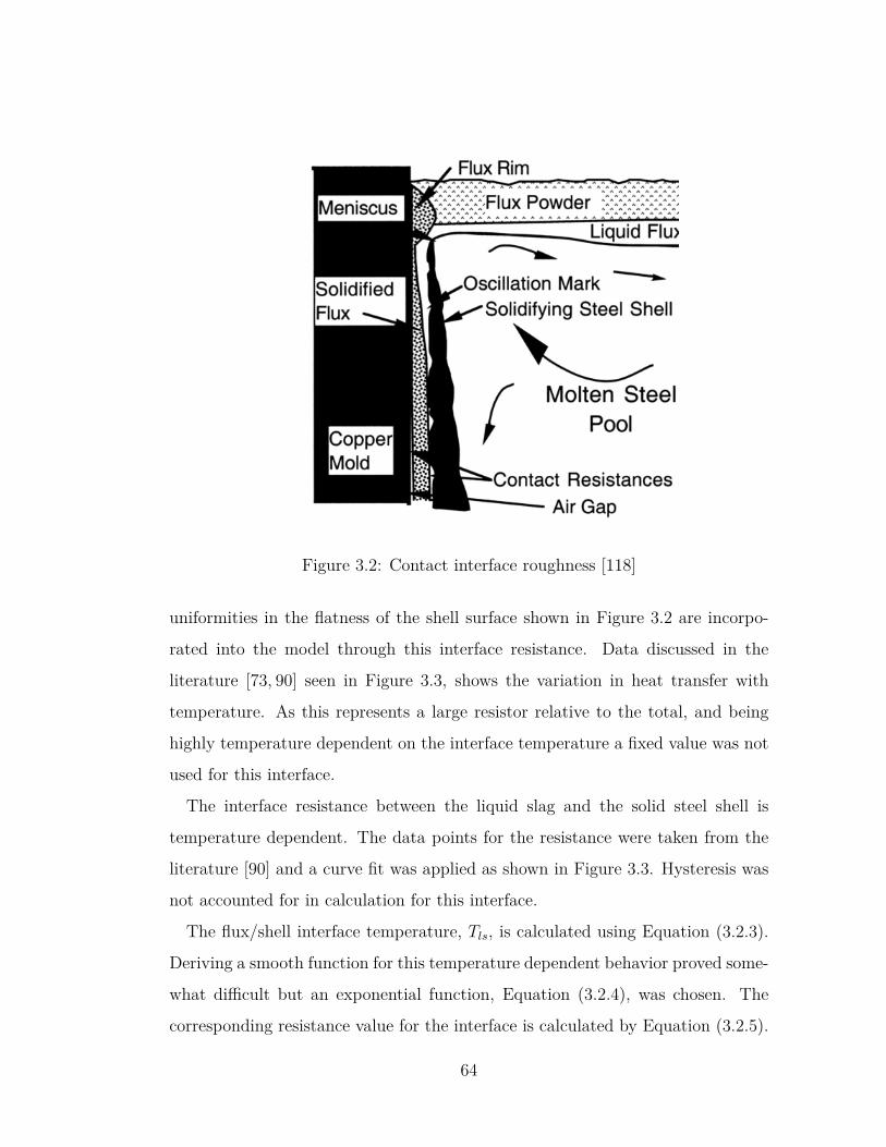
Figure 3.2: Contact interface roughness [118]

uniformities in the flatness of the shell surface shown in Figure 3.2 are incorpo-

rated into the model through this interface resistance. Data discussed in the

literature [73, 90] seen in Figure 3.3, shows the variation in heat transfer with

temperature. As this represents a large resistor relative to the total, and being

highly temperature dependent on the interface temperature a fixed value was not

used for this interface.

The interface resistance between the liquid slag and the solid steel shell is

temperature dependent. The data points for the resistance were taken from the

literature [90] and a curve fit was applied as shown in Figure 3.3. Hysteresis was

not accounted for in calculation for this interface.

The flux/shell interface temperature, Tls, is calculated using Equation (3.2.3).

Deriving a smooth function for this temperature dependent behavior proved some-

what difficult but an exponential function, Equation (3.2.4), was chosen. The

corresponding resistance value for the interface is calculated by Equation (3.2.5).

64

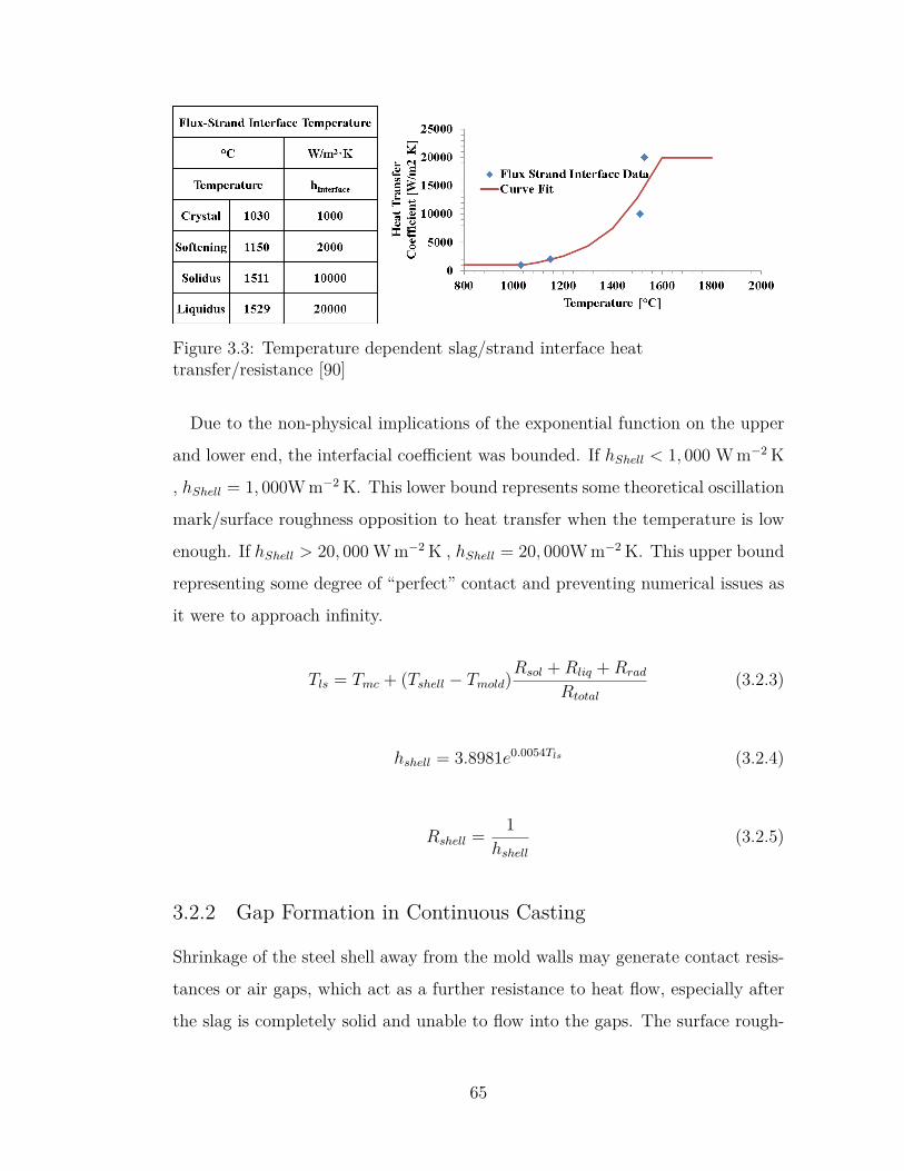
Figure 3.3: Temperature dependent slag/strand interface heattransfer/resistance [90]

Due to the non-physical implications of the exponential function on the upper

and lower end, the interfacial coefficient was bounded. If hShell < 1, 000 W m−2 K

, hShell = 1, 000W m−2 K. This lower bound represents some theoretical oscillation

mark/surface roughness opposition to heat transfer when the temperature is low

enough. If hShell > 20, 000 W m−2 K , hShell = 20, 000W m−2 K. This upper bound

representing some degree of “perfect” contact and preventing numerical issues as

it were to approach infinity.

Tls = Tmc + (Tshell − Tmold)Rsol +Rliq +Rrad

Rtotal

(3.2.3)

hshell = 3.8981e0.0054Tls (3.2.4)

Rshell = 1hshell

(3.2.5)

3.2.2 Gap Formation in Continuous Casting

Shrinkage of the steel shell away from the mold walls may generate contact resis-

tances or air gaps, which act as a further resistance to heat flow, especially after

the slag is completely solid and unable to flow into the gaps. The surface rough-

65

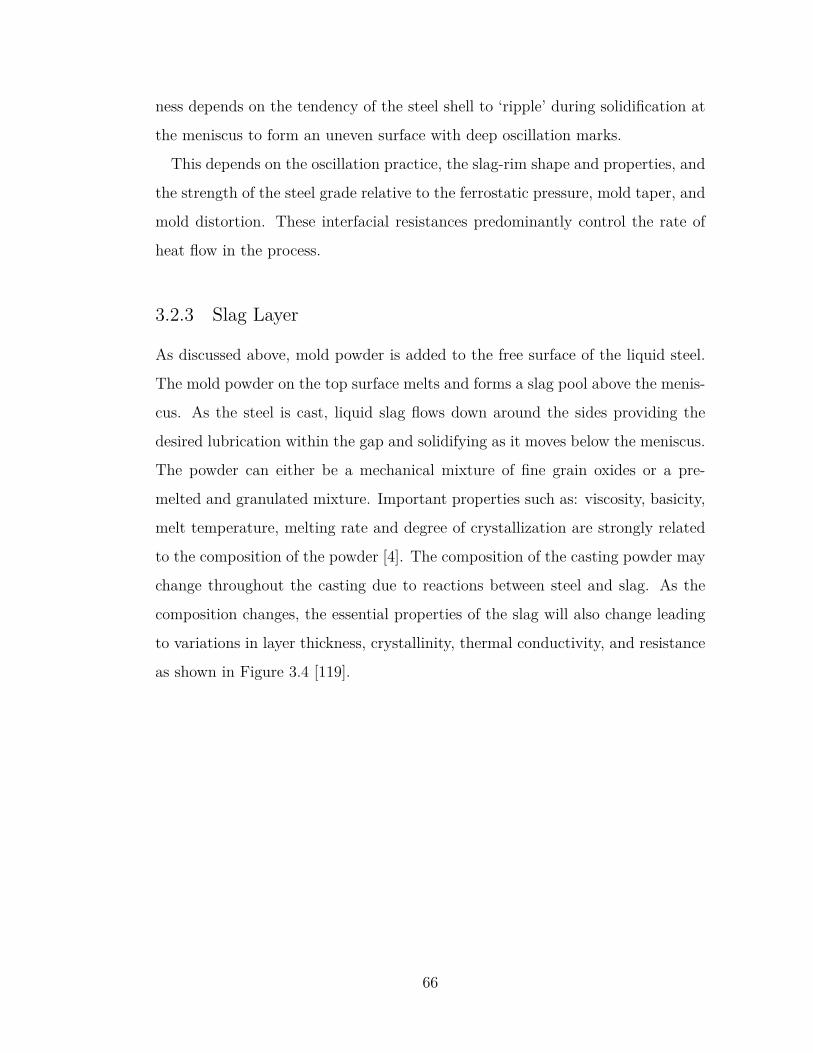
ness depends on the tendency of the steel shell to ‘ripple’ during solidification at

the meniscus to form an uneven surface with deep oscillation marks.

This depends on the oscillation practice, the slag-rim shape and properties, and

the strength of the steel grade relative to the ferrostatic pressure, mold taper, and

mold distortion. These interfacial resistances predominantly control the rate of

heat flow in the process.

3.2.3 Slag Layer

As discussed above, mold powder is added to the free surface of the liquid steel.

The mold powder on the top surface melts and forms a slag pool above the menis-

cus. As the steel is cast, liquid slag flows down around the sides providing the

desired lubrication within the gap and solidifying as it moves below the meniscus.

The powder can either be a mechanical mixture of fine grain oxides or a pre-

melted and granulated mixture. Important properties such as: viscosity, basicity,

melt temperature, melting rate and degree of crystallization are strongly related

to the composition of the powder [4]. The composition of the casting powder may

change throughout the casting due to reactions between steel and slag. As the

composition changes, the essential properties of the slag will also change leading

to variations in layer thickness, crystallinity, thermal conductivity, and resistance

as shown in Figure 3.4 [119].

66

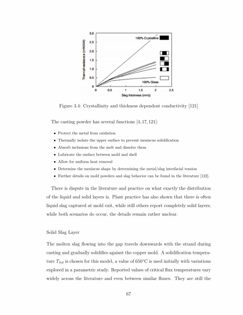
Figure 3.4: Crystallinity and thickness dependent conductivity [121]

The casting powder has several functions [4, 17,121]:

• Protect the metal from oxidation

• Thermally isolate the upper surface to prevent meniscus solidification

• Absorb inclusions from the melt and dissolve them

• Lubricate the surface between mold and shell

• Allow for uniform heat removal

• Determine the meniscus shape by determining the metal/slag interfacial tension

• Further details on mold powders and slag behavior can be found in the literature [122].

There is dispute in the literature and practice on what exactly the distribution

of the liquid and solid layers is. Plant practice has also shown that there is often

liquid slag captured at mold exit, while still others report completely solid layers;

while both scenarios do occur, the details remain rather unclear.

Solid Slag Layer

The molten slag flowing into the gap travels downwards with the strand during

casting and gradually solidifies against the copper mold. A solidification tempera-

ture TSol is chosen for this model, a value of 650◦C is used initially with variations

explored in a parametric study. Reported values of critical flux temperatures vary

widely across the literature and even between similar fluxes. They are still the

67

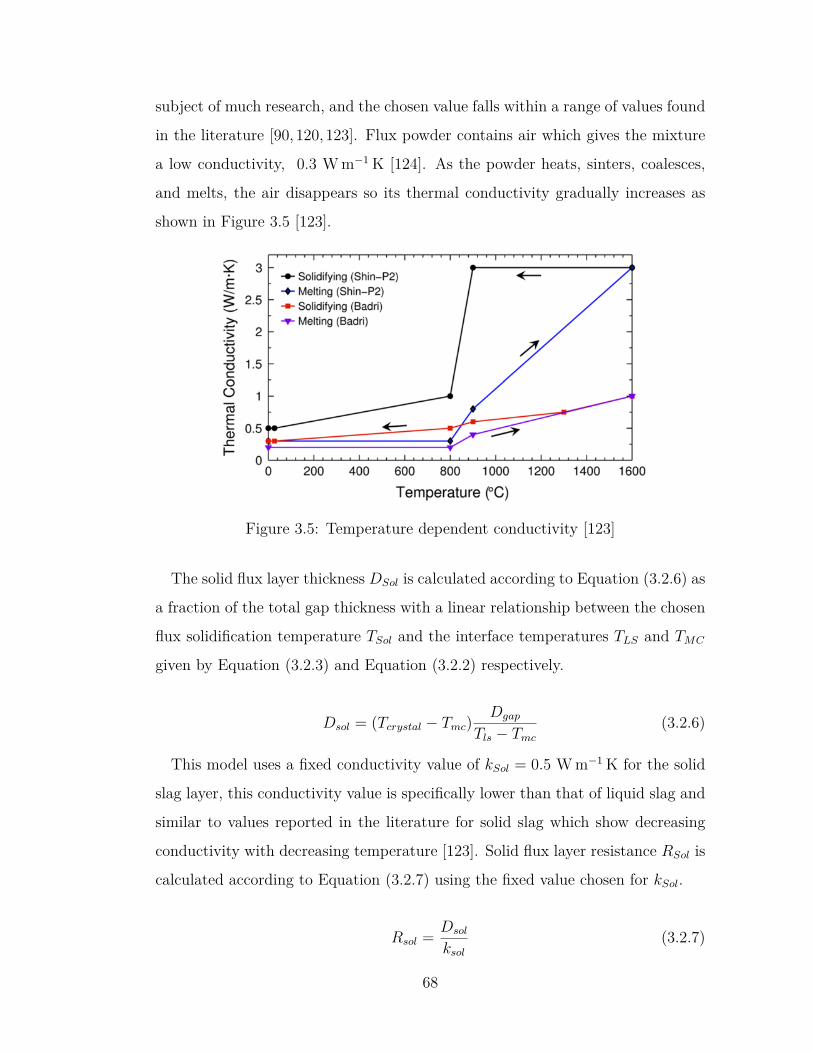
subject of much research, and the chosen value falls within a range of values found

in the literature [90, 120, 123]. Flux powder contains air which gives the mixture

a low conductivity, 0.3 W m−1 K [124]. As the powder heats, sinters, coalesces,

and melts, the air disappears so its thermal conductivity gradually increases as

shown in Figure 3.5 [123].

Figure 3.5: Temperature dependent conductivity [123]

The solid flux layer thickness DSol is calculated according to Equation (3.2.6) as

a fraction of the total gap thickness with a linear relationship between the chosen

flux solidification temperature TSol and the interface temperatures TLS and TMC

given by Equation (3.2.3) and Equation (3.2.2) respectively.

Dsol = (Tcrystal − Tmc)Dgap

Tls − Tmc(3.2.6)

This model uses a fixed conductivity value of kSol = 0.5 W m−1 K for the solid

slag layer, this conductivity value is specifically lower than that of liquid slag and

similar to values reported in the literature for solid slag which show decreasing

conductivity with decreasing temperature [123]. Solid flux layer resistance RSol is

calculated according to Equation (3.2.7) using the fixed value chosen for kSol.

Rsol = Dsol

ksol(3.2.7)

68

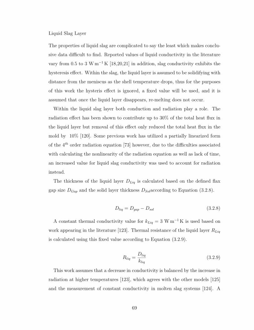
Liquid Slag Layer

The properties of liquid slag are complicated to say the least which makes conclu-

sive data difficult to find. Reported values of liquid conductivity in the literature

vary from 0.5 to 3 W m−1 K [18,20,21] in addition, slag conductivity exhibits the

hysteresis effect. Within the slag, the liquid layer is assumed to be solidifying with

distance from the meniscus as the shell temperature drops, thus for the purposes

of this work the hysteris effect is ignored, a fixed value will be used, and it is

assumed that once the liquid layer disappears, re-melting does not occur.

Within the liquid slag layer both conduction and radiation play a role. The

radiation effect has been shown to contribute up to 30% of the total heat flux in

the liquid layer but removal of this effect only reduced the total heat flux in the

mold by 10% [120]. Some previous work has utilized a partially linearized form

of the 4th order radiation equation [73] however, due to the difficulties associated

with calculating the nonlinearity of the radiation equation as well as lack of time,

an increased value for liquid slag conductivity was used to account for radiation

instead.

The thickness of the liquid layer DLiq is calculated based on the defined flax

gap size DGap and the solid layer thickness DSolaccording to Equation (3.2.8).

Dliq = Dgap −Dsol (3.2.8)

A constant thermal conductivity value for kLiq = 3 W m−1 K is used based on

work appearing in the literature [123]. Thermal resistance of the liquid layer RLiq

is calculated using this fixed value according to Equation (3.2.9).

Rliq = Dliq

kliq(3.2.9)

This work assumes that a decrease in conductivity is balanced by the increase in

radiation at higher temperatures [123], which agrees with the other models [125]

and the measurement of constant conductivity in molten slag systems [124]. A

69

minimum threshold value for liquid layer thickness is chosen to ease numerical dif-

ficulties and prevent wildly large values for heat transfer coefficient. This thickness

DLiquidThresh is chosen to be 0.01mm for this work which represents a maximum

h value to be 20, 000 W m−2 K, values used in the literature have been in this

range [73].

3.2.4 The Air Gap

As discussed previously, if conditions within the mold allow for it, an air gap

can form. The size of the air gap is an output of the stress model in the form

of displacement of the shell surface nodes from the mold. This model includes

time dependent ferrostatic pressure applied as a traction pulling the shell towards

the mold surface. To help the numerical solution a minimum threshold value

DAirThresh = 0.001 mm is adopted to prevent non-physical behavior associated

with very small gaps (displacements). The details of the ferrostatic pressure

method are the same as that described in Appendix A.1.

Additionally, if there is a liquid layer of slag present in the gap above the chosen

TSol temperature, the air gap is given to be filled with liquid slag. This condition

is based on the assumption that liquid slag from above the gap location would

flow downwards to fill in this gap.

The thermal conductivity of the air gap is dependent on composition of the gas

[126]. Prior work has values assumed for air [90] as well as a 20% hydrogen mixture

[126] using the binary conductivity mixture rules [127]. For this work a fixed value

for conductivity kAir = 0.06 W m−1 K is used for the air gap [85]. This value is

consistent with low temperature values for a high hydrogen environment found in

the literature [126]. A temperature dependent conductivity value is left for future

work. The thermal resistance of the air gap is given by Equation (3.2.10).

RAir = DAir

0.06 (3.2.10)

70

3.2.5 Total Gap Heat Transfer

The heat transfer model is dependent on the 5 resistant components in the gap

described above: the mold/slag interface, the air gap, the solid slag layer, the liq-

uid slag layer, and the slag/steel interface. Combining Equations (3.2.1), (3.2.5),

(3.2.7), (3.2.9) and (3.2.10) into Equation (3.2.11) yields Equation (3.2.12) and

an effective thermal resistor model represented by Figures 3.6 and 3.7.

Heat conduction depends on the thermal resistances and time-averaged thick-

ness profiles down the mold of the different layers of materials contained in the

gap. For the purposes of this model, we are concerned primarily with the bulk

behavior of the solidifying shell. as such a number of simplifications will be made:

In addition to those discussed above, some simplifying assumptions were made

for this model:

• The potential buildup of scale, and/or resulting blockage, within the water

channels was neglected, thus we will assume that the mold is operating at

steady state with constant temperature TMold = 150◦C

• The distribution of liquid and solid slag will be assumed linear between the

interface temperatures

• As mold slags are mixtures they do not have a singular transition tempera-

ture. While there is some debate on the minimum percentage of liquid slag

that would fill in an air gap, for the purposes of this work, 60% liquid slag

will be assumed to fill in an air gap.

• The latent heat evolved by liquid-slag solidification is less than 3% of the

heat transferred across the gap, so it is neglected in this model. [96]

• Oscillation marks and prescribed surface shape non-uniformity are neglected

• Interface resistances are not dependent on flux layer thickness

71

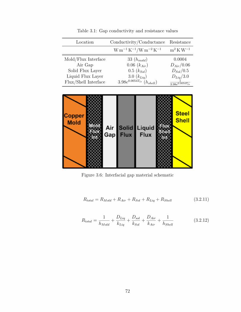
Table 3.1: Gap conductivity and resistance values

Location Conductivity/Conductance ResistanceW m−1 K−1/W m−2 K−1 m2 K W−1

Mold/Flux Interface 33 (hmold) 0.0004Air Gap 0.06 (kAir) DAir/0.06

Solid Flux Layer 0.5 (kSol) DSol/0.5Liquid Flux Layer 3.0 (kLiq) DLiq/3.0Flux/Shell Interface 3.98e0.0054Tls (hshell) 1

3.98e0.0054Tls

Figure 3.6: Interfacial gap material schematic

Rtotal = RMold +RAir +RSol +RLiq +RShell (3.2.11)

Rtotal = 1hMold

+ DLiq

kLiq+ Dsol

kSol+ DAir

kAir+ 1hShell

(3.2.12)

72

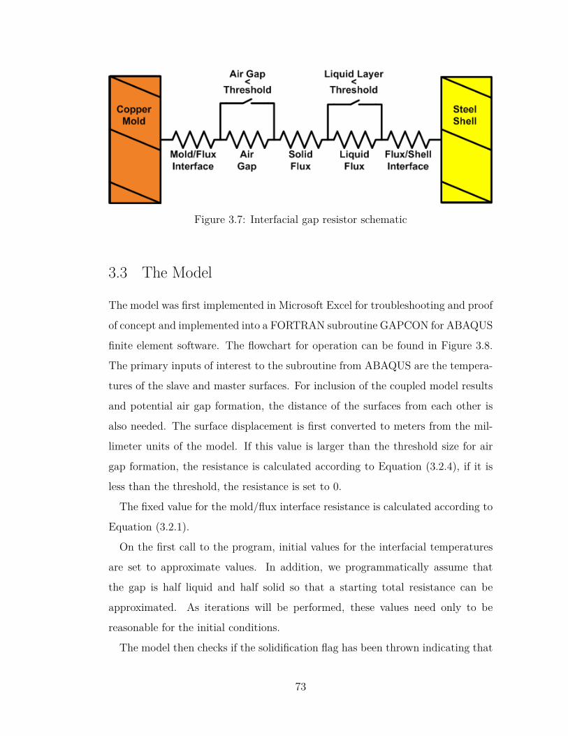
Figure 3.7: Interfacial gap resistor schematic

3.3 The Model

The model was first implemented in Microsoft Excel for troubleshooting and proof

of concept and implemented into a FORTRAN subroutine GAPCON for ABAQUS

finite element software. The flowchart for operation can be found in Figure 3.8.

The primary inputs of interest to the subroutine from ABAQUS are the tempera-

tures of the slave and master surfaces. For inclusion of the coupled model results

and potential air gap formation, the distance of the surfaces from each other is

also needed. The surface displacement is first converted to meters from the mil-

limeter units of the model. If this value is larger than the threshold size for air

gap formation, the resistance is calculated according to Equation (3.2.4), if it is

less than the threshold, the resistance is set to 0.

The fixed value for the mold/flux interface resistance is calculated according to

Equation (3.2.1).

On the first call to the program, initial values for the interfacial temperatures

are set to approximate values. In addition, we programmatically assume that

the gap is half liquid and half solid so that a starting total resistance can be

approximated. As iterations will be performed, these values need only to be

reasonable for the initial conditions.

The model then checks if the solidification flag has been thrown indicating that

73

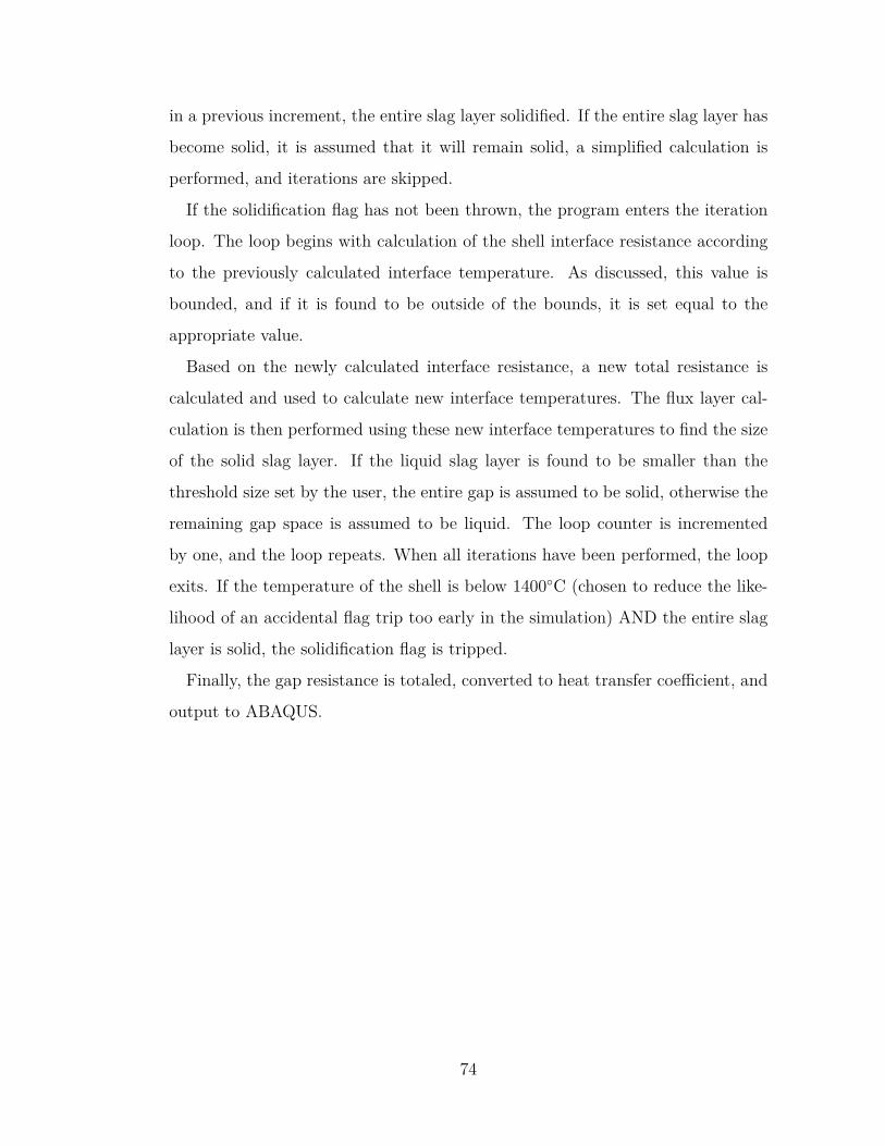
in a previous increment, the entire slag layer solidified. If the entire slag layer has

become solid, it is assumed that it will remain solid, a simplified calculation is

performed, and iterations are skipped.

If the solidification flag has not been thrown, the program enters the iteration

loop. The loop begins with calculation of the shell interface resistance according

to the previously calculated interface temperature. As discussed, this value is

bounded, and if it is found to be outside of the bounds, it is set equal to the

appropriate value.

Based on the newly calculated interface resistance, a new total resistance is

calculated and used to calculate new interface temperatures. The flux layer cal-

culation is then performed using these new interface temperatures to find the size

of the solid slag layer. If the liquid slag layer is found to be smaller than the

threshold size set by the user, the entire gap is assumed to be solid, otherwise the

remaining gap space is assumed to be liquid. The loop counter is incremented

by one, and the loop repeats. When all iterations have been performed, the loop

exits. If the temperature of the shell is below 1400◦C (chosen to reduce the like-

lihood of an accidental flag trip too early in the simulation) AND the entire slag

layer is solid, the solidification flag is tripped.

Finally, the gap resistance is totaled, converted to heat transfer coefficient, and

output to ABAQUS.

74

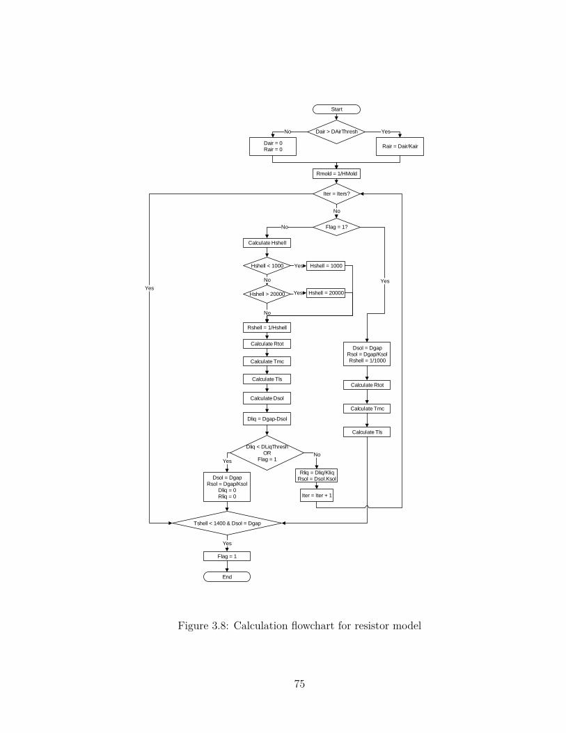
Dair > DAirThresh

Flag = 1?

Iter = Iters?

Iter = Iter + 1

Flag = 1

Start

End

Calculate Rtot

Calculate Hshell

Calculate Tls

Calculate Tmc

Yes

Dsol = DgapRsol = Dgap/Ksol

Dliq = 0Rliq = 0

Yes

Dair = 0Rair = 0

Rair = Dair/Kair

YesNo

Rmold = 1/HMold

Dsol = DgapRsol = Dgap/KsolRshell = 1/1000

Tshell < 1400 & Dsol = Dgap

Yes

Hshell = 1000

Hshell = 20000

Rshell = 1/Hshell

Calculate Dsol

Dliq = Dgap-Dsol

Dliq < DLiqThreshOR

Flag = 1

Rliq = Dliq/KliqRsol = Dsol.Ksol

No

No

No

Calculate Rtot

Calculate Tls

Calculate Tmc

Yes

Hshell < 1000

Hshell > 20000

Yes

No

Yes

No

Figure 3.8: Calculation flowchart for resistor model

75

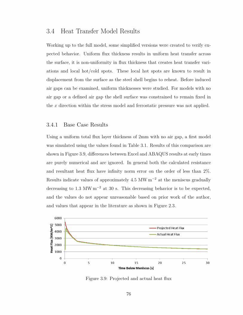
3.4 Heat Transfer Model Results

Working up to the full model, some simplified versions were created to verify ex-

pected behavior. Uniform flux thickness results in uniform heat transfer across

the surface, it is non-uniformity in flux thickness that creates heat transfer vari-

ations and local hot/cold spots. These local hot spots are known to result in

displacement from the surface as the steel shell begins to reheat. Before induced

air gaps can be examined, uniform thicknesses were studied. For models with no

air gap or a defined air gap the shell surface was constrained to remain fixed in

the x direction within the stress model and ferrostatic pressure was not applied.

3.4.1 Base Case Results

Using a uniform total flux layer thickness of 2mm with no air gap, a first model

was simulated using the values found in Table 3.1. Results of this comparison are

shown in Figure 3.9, differences between Excel and ABAQUS results at early times

are purely numerical and are ignored. In general both the calculated resistance

and resultant heat flux have infinity norm error on the order of less than 2%.

Results indicate values of approximately 4.5 MW m−2 at the meniscus gradually

decreasing to 1.3 MW m−2 at 30 s. This decreasing behavior is to be expected,

and the values do not appear unreasonable based on prior work of the author,

and values that appear in the literature as shown in Figure 2.3.

Figure 3.9: Projected and actual heat flux

76

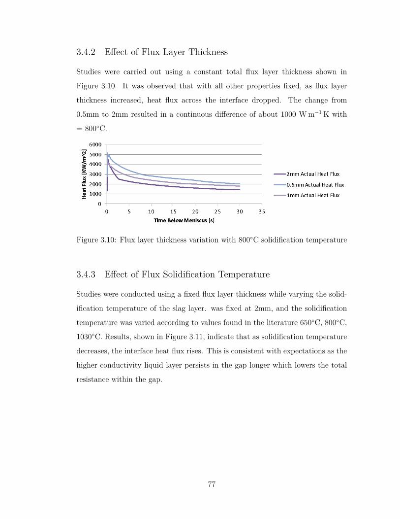
3.4.2 Effect of Flux Layer Thickness

Studies were carried out using a constant total flux layer thickness shown in

Figure 3.10. It was observed that with all other properties fixed, as flux layer

thickness increased, heat flux across the interface dropped. The change from

0.5mm to 2mm resulted in a continuous difference of about 1000 W m−1 K with

= 800◦C.

Figure 3.10: Flux layer thickness variation with 800◦C solidification temperature

3.4.3 Effect of Flux Solidification Temperature

Studies were conducted using a fixed flux layer thickness while varying the solid-

ification temperature of the slag layer. was fixed at 2mm, and the solidification

temperature was varied according to values found in the literature 650◦C, 800◦C,

1030◦C. Results, shown in Figure 3.11, indicate that as solidification temperature

decreases, the interface heat flux rises. This is consistent with expectations as the

higher conductivity liquid layer persists in the gap longer which lowers the total

resistance within the gap.

77

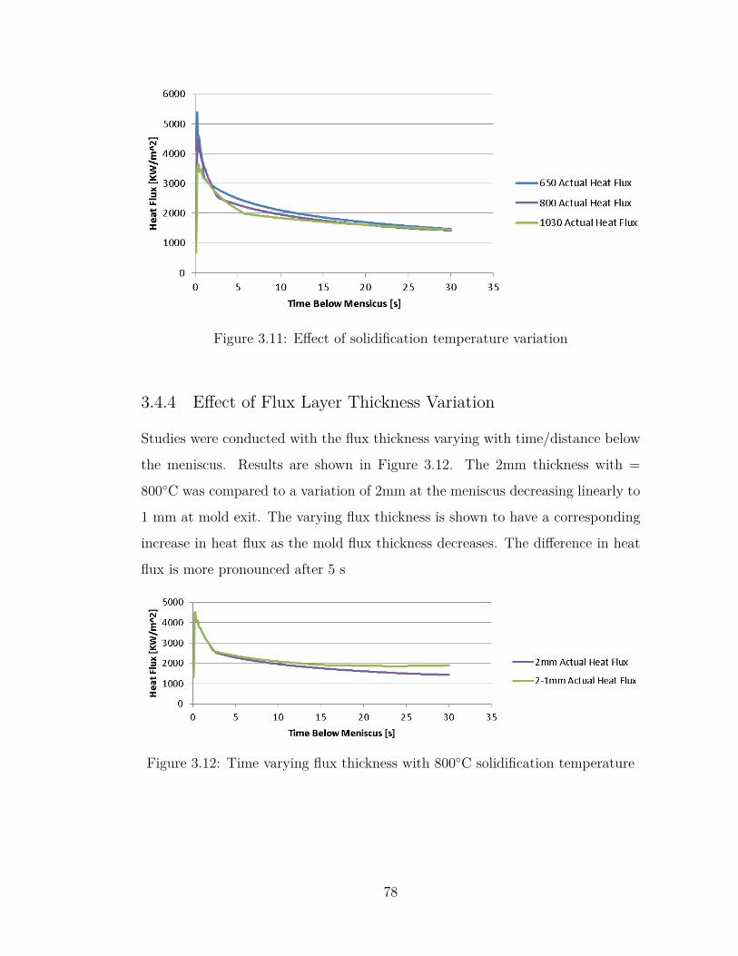
Figure 3.11: Effect of solidification temperature variation

3.4.4 Effect of Flux Layer Thickness Variation

Studies were conducted with the flux thickness varying with time/distance below

the meniscus. Results are shown in Figure 3.12. The 2mm thickness with =

800◦C was compared to a variation of 2mm at the meniscus decreasing linearly to

1 mm at mold exit. The varying flux thickness is shown to have a corresponding

increase in heat flux as the mold flux thickness decreases. The difference in heat

flux is more pronounced after 5 s

Figure 3.12: Time varying flux thickness with 800◦C solidification temperature

78

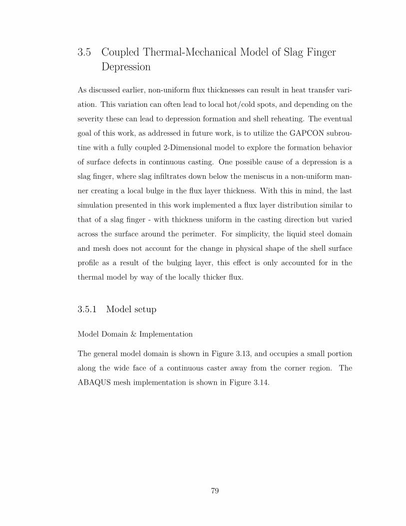
3.5 Coupled Thermal-Mechanical Model of Slag FingerDepression

As discussed earlier, non-uniform flux thicknesses can result in heat transfer vari-

ation. This variation can often lead to local hot/cold spots, and depending on the

severity these can lead to depression formation and shell reheating. The eventual

goal of this work, as addressed in future work, is to utilize the GAPCON subrou-

tine with a fully coupled 2-Dimensional model to explore the formation behavior

of surface defects in continuous casting. One possible cause of a depression is a

slag finger, where slag infiltrates down below the meniscus in a non-uniform man-

ner creating a local bulge in the flux layer thickness. With this in mind, the last

simulation presented in this work implemented a flux layer distribution similar to

that of a slag finger - with thickness uniform in the casting direction but varied

across the surface around the perimeter. For simplicity, the liquid steel domain

and mesh does not account for the change in physical shape of the shell surface

profile as a result of the bulging layer, this effect is only accounted for in the

thermal model by way of the locally thicker flux.

3.5.1 Model setup

Model Domain & Implementation

The general model domain is shown in Figure 3.13, and occupies a small portion

along the wide face of a continuous caster away from the corner region. The

ABAQUS mesh implementation is shown in Figure 3.14.

79

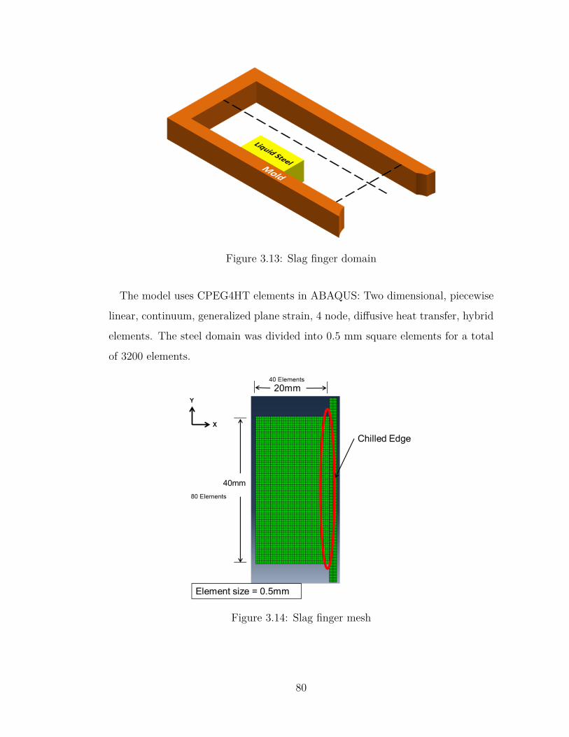
Figure 3.13: Slag finger domain

The model uses CPEG4HT elements in ABAQUS: Two dimensional, piecewise

linear, continuum, generalized plane strain, 4 node, diffusive heat transfer, hybrid

elements. The steel domain was divided into 0.5 mm square elements for a total

of 3200 elements.

Figure 3.14: Slag finger mesh

80

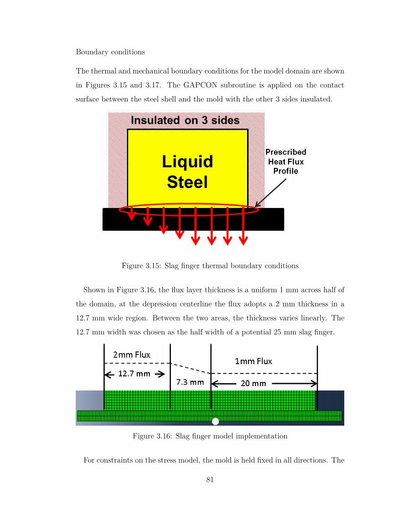
Boundary conditions

The thermal and mechanical boundary conditions for the model domain are shown

in Figures 3.15 and 3.17. The GAPCON subroutine is applied on the contact

surface between the steel shell and the mold with the other 3 sides insulated.

Figure 3.15: Slag finger thermal boundary conditions

Shown in Figure 3.16, the flux layer thickness is a uniform 1 mm across half of

the domain, at the depression centerline the flux adopts a 2 mm thickness in a

12.7 mm wide region. Between the two areas, the thickness varies linearly. The

12.7 mm width was chosen as the half width of a potential 25 mm slag finger.

Figure 3.16: Slag finger model implementation

For constraints on the stress model, the mold is held fixed in all directions. The

81

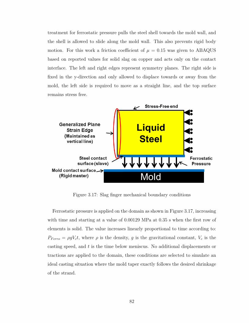
treatment for ferrostatic pressure pulls the steel shell towards the mold wall, and

the shell is allowed to slide along the mold wall. This also prevents rigid body

motion. For this work a friction coefficient of µ = 0.15 was given to ABAQUS

based on reported values for solid slag on copper and acts only on the contact

interface. The left and right edges represent symmetry planes. The right side is

fixed in the y-direction and only allowed to displace towards or away from the

mold, the left side is required to move as a straight line, and the top surface

remains stress free.

Figure 3.17: Slag finger mechanical boundary conditions

Ferrostatic pressure is applied on the domain as shown in Figure 3.17, increasing

with time and starting at a value of 0.00129 MPa at 0.35 s when the first row of

elements is solid. The value increases linearly proportional to time according to:

PFerro = ρgVct, where ρ is the density, g is the gravitational constant, Vc is the

casting speed, and t is the time below meniscus. No additional displacements or

tractions are applied to the domain, these conditions are selected to simulate an

ideal casting situation where the mold taper exactly follows the desired shrinkage

of the strand.

82

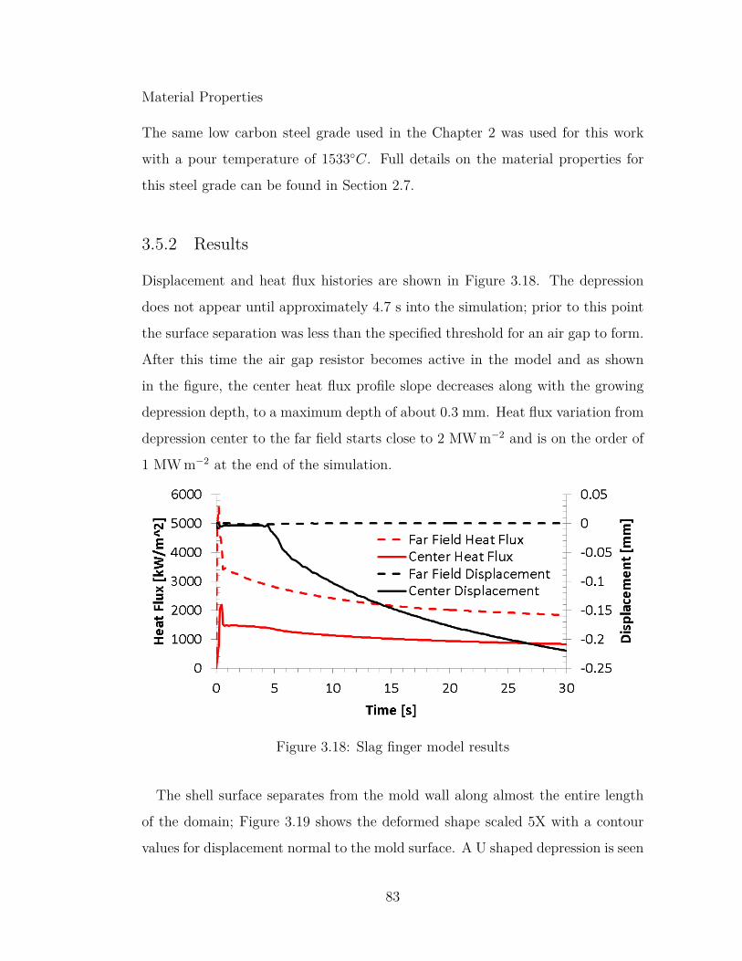
Material Properties

The same low carbon steel grade used in the Chapter 2 was used for this work

with a pour temperature of 1533◦C. Full details on the material properties for

this steel grade can be found in Section 2.7.

3.5.2 Results

Displacement and heat flux histories are shown in Figure 3.18. The depression

does not appear until approximately 4.7 s into the simulation; prior to this point

the surface separation was less than the specified threshold for an air gap to form.

After this time the air gap resistor becomes active in the model and as shown

in the figure, the center heat flux profile slope decreases along with the growing

depression depth, to a maximum depth of about 0.3 mm. Heat flux variation from

depression center to the far field starts close to 2 MW m−2 and is on the order of

1 MW m−2 at the end of the simulation.

Figure 3.18: Slag finger model results

The shell surface separates from the mold wall along almost the entire length

of the domain; Figure 3.19 shows the deformed shape scaled 5X with a contour

values for displacement normal to the mold surface. A U shaped depression is seen

83

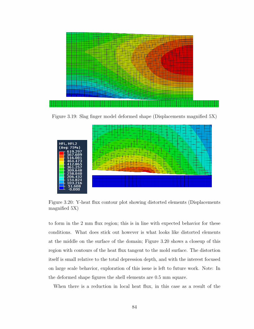
Figure 3.19: Slag finger model deformed shape (Displacements magnified 5X)

Figure 3.20: Y-heat flux contour plot showing distorted elements (Displacementsmagnified 5X)

to form in the 2 mm flux region; this is in line with expected behavior for these

conditions. What does stick out however is what looks like distorted elements

at the middle on the surface of the domain; Figure 3.20 shows a closeup of this

region with contours of the heat flux tangent to the mold surface. The distortion

itself is small relative to the total depression depth, and with the interest focused

on large scale behavior, exploration of this issue is left to future work. Note: In

the deformed shape figures the shell elements are 0.5 mm square.

When there is a reduction in local heat flux, in this case as a result of the

84

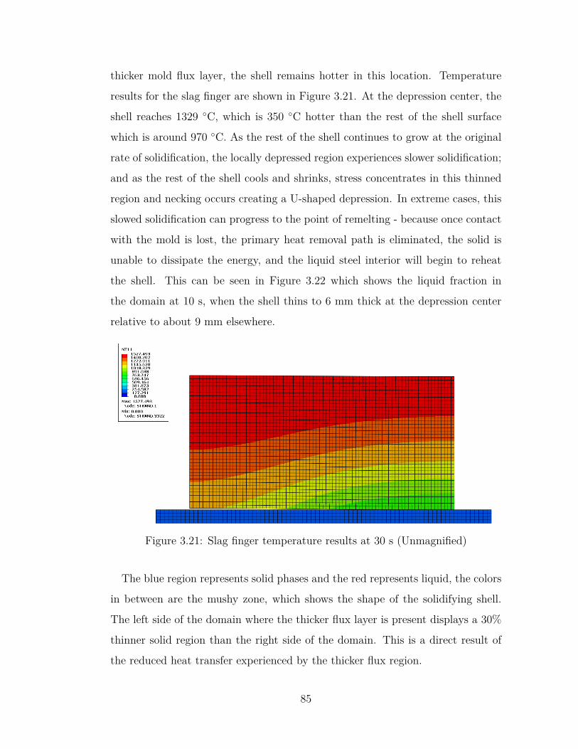
thicker mold flux layer, the shell remains hotter in this location. Temperature

results for the slag finger are shown in Figure 3.21. At the depression center, the

shell reaches 1329 ◦C, which is 350 ◦C hotter than the rest of the shell surface

which is around 970 ◦C. As the rest of the shell continues to grow at the original

rate of solidification, the locally depressed region experiences slower solidification;

and as the rest of the shell cools and shrinks, stress concentrates in this thinned

region and necking occurs creating a U-shaped depression. In extreme cases, this

slowed solidification can progress to the point of remelting - because once contact

with the mold is lost, the primary heat removal path is eliminated, the solid is

unable to dissipate the energy, and the liquid steel interior will begin to reheat

the shell. This can be seen in Figure 3.22 which shows the liquid fraction in

the domain at 10 s, when the shell thins to 6 mm thick at the depression center

relative to about 9 mm elsewhere.

Figure 3.21: Slag finger temperature results at 30 s (Unmagnified)

The blue region represents solid phases and the red represents liquid, the colors

in between are the mushy zone, which shows the shape of the solidifying shell.

The left side of the domain where the thicker flux layer is present displays a 30%

thinner solid region than the right side of the domain. This is a direct result of

the reduced heat transfer experienced by the thicker flux region.

85

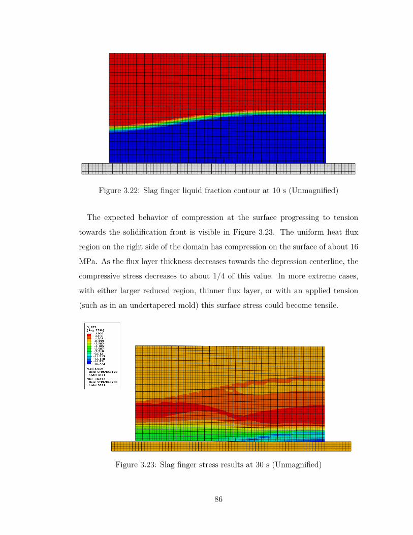
Figure 3.22: Slag finger liquid fraction contour at 10 s (Unmagnified)

The expected behavior of compression at the surface progressing to tension

towards the solidification front is visible in Figure 3.23. The uniform heat flux

region on the right side of the domain has compression on the surface of about 16

MPa. As the flux layer thickness decreases towards the depression centerline, the

compressive stress decreases to about 1/4 of this value. In more extreme cases,

with either larger reduced region, thinner flux layer, or with an applied tension

(such as in an undertapered mold) this surface stress could become tensile.

Figure 3.23: Slag finger stress results at 30 s (Unmagnified)

86

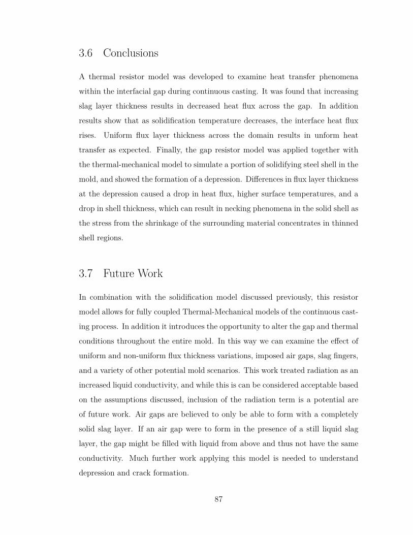
3.6 Conclusions

A thermal resistor model was developed to examine heat transfer phenomena

within the interfacial gap during continuous casting. It was found that increasing

slag layer thickness results in decreased heat flux across the gap. In addition

results show that as solidification temperature decreases, the interface heat flux

rises. Uniform flux layer thickness across the domain results in unform heat

transfer as expected. Finally, the gap resistor model was applied together with

the thermal-mechanical model to simulate a portion of solidifying steel shell in the

mold, and showed the formation of a depression. Differences in flux layer thickness

at the depression caused a drop in heat flux, higher surface temperatures, and a

drop in shell thickness, which can result in necking phenomena in the solid shell as

the stress from the shrinkage of the surrounding material concentrates in thinned

shell regions.

3.7 Future Work

In combination with the solidification model discussed previously, this resistor

model allows for fully coupled Thermal-Mechanical models of the continuous cast-

ing process. In addition it introduces the opportunity to alter the gap and thermal

conditions throughout the entire mold. In this way we can examine the effect of

uniform and non-uniform flux thickness variations, imposed air gaps, slag fingers,

and a variety of other potential mold scenarios. This work treated radiation as an

increased liquid conductivity, and while this is can be considered acceptable based

on the assumptions discussed, inclusion of the radiation term is a potential are

of future work. Air gaps are believed to only be able to form with a completely

solid slag layer. If an air gap were to form in the presence of a still liquid slag

layer, the gap might be filled with liquid from above and thus not have the same

conductivity. Much further work applying this model is needed to understand

depression and crack formation.

87

Chapter 4

Conclusions and Future Work

4.1 Conclusions

This work has developed and demonstrated 3 mathematical models in an effort

to examine thermal and mechanical behavior in the mold region of the continu-

ous casting process. A semi-one-dimensional model has been developed to study

the effect of changes in steel grade early in the solidification process. General

behavior has been discussed and explored, and similarities and differences have

been noted. A thermal resistor model of the interfacial gap was developed to

enable future coupled modeling work to extend this model into defect formation

such as longitudinal cracks. Finally, these models have been combined into a two-

dimensional model to explore depression formation and the effects of heat transfer

variation across the surface of the mold.

Four different steel grades were investigated: Ultra-Low Carbon (0.003 %C),

Low Carbon (0.04 %C), Peritectic (0.13 %C), and High Carbon (0.47 %C), sim-

ulating 30 s dwell times. Mesh refinement for capturing solidification details was

examined and element sizes of 0.1 mm or smaller may be required to properly

study solidification phenomena. All steel grades were found to follow the same

general solidification behavior of compression at the surface increasing with time,

and tension towards the solidification front. The initial solidification rate increases

with carbon content. Thermal strain dominates the mechanical behavior. More

stress and inelastic strain are generated in the high carbon steels, because they

are mainly composed of high-strength austenite. Stress in the δ-ferrite phase is

always very small, owing to the low strength of this phase. This simple model can

88

help in the calculation of taper profiles for different steel grades and maintain the

desired contact with the mold. While fixed linear taper practices are common in

industry, this work demonstrates that the desired profile of the shell is actually

parabolic.

A thermal resistor model was developed to examine heat transfer phenomena

within the interfacial gap during continuous casting. It was found that increasing

slag layer thickness results in decreased heat flux across the gap. In addition

results show that as solidification temperature decreases, the interface heat flux

rises. Uniform flux layer thickness across the domain results in unform heat

transfer as expected.

Finally, this work has demonstrated an example of combining the realistic

thermal-resistor model of the gap together with the thermal-mechanical model

to show the different local behavior that can occur at a depression. Differences in

flux layer thickness at the depression caused a drop in heat flux, higher surface

temperatures, and a drop in shell thickness, which can result in necking phenom-

ena in the solid shell as the stress from the shrinkage of the surrounding material

concentrates in thinned shell regions.

This work demonstrates the methodology necessary to model and capture the

relevant behavior in a solidification problem; it also explores the basic property

differences between steel grades according to the phase fractions and the properties

of each phase, presents validation using analytical solutions, and a simulation of

a continuous thin slab steel casting process where the shrinkage and solidification

behavior of each grade is explored.

The increasing pressure and demands of the industry mean that new tools

will always need to be developed to help expand and extrapolate our existing

knowledge to keep up the pace. Increases in throughput are always a goal of

manufacturers as long as it can be done effectively, without a loss of quality, and

(especially in the case of steel plant operations) safely. With the information these

models provide, better decisions, safer operating practices, and higher casting

speeds can be realized.

89

In addition, it is the first step in demonstrating a transient 3-D model of

thermal-mechanical behavior to examine the formation of cracks and depressions -

where the correct behavior can be verified in a simplified case where an analytical

solution exists, while allowing for extensions to higher dimensional modeling work

in the future.

4.2 Future Work

The models developed in this work already provide a useful predictive tool and

extensions of them will only increase their utility. The macroscopic models of

thermal-mechanical behavior presented here should be combined together and

applied to the entire strand. Next, more microscale behavior should be imple-

mented, such as anisotropic behavior, cooling rate dependency. Then, in order to

predict crack formation, damage criteria should be included. The detailed model

used to investigate a single depression should be extended to investigate differ-

ent cases, including grade variation, in order to identify the mechanisms for how

individual depression-shaped defects are formed.

As mentioned previously, the complexities of the interfacial gap region make it

quite difficult to study and model. In reality many of the conductivities and resis-

tances are cooling rate based in addition to temperature dependency; furthermore

the flux layer may be squeezed around and redistribute itself within the mold -

implement better model for slag behavior in the gap by including for example the

effect of flow due to squeezing when shell is forced against the mold, such as when

taper is too high.

In the future a full quarter symmetry model of a slab may be used to examine

the large scale behavior especially in the corner region, in addition, allowing the

mold surface to distort within the model or including an already deformed mold

shape may allows for study of asymmetries that otherwise may not have been

seen.

The models developed in this work provide a useful starting point for exam-

90

ining continuous casting solidification. However, there is still a large gap in the

ability to predict the formation of cracks and depressions, and missing knowledge

regarding the crack sensitivity of peritectic steels. Breakouts at operating casters

are extremely expensive and dangerous. Finding ways to understand and solve

the root causes behind cracks and depressions, as well as the complexities of peri-

tectics and newer grades, will lead to reductions in breakouts which will both save

money and operational downtime, but more importantly keep employees safe.

91

Appendix A

Ferrostatic Pressure

A.1 Ferrostatic Pressure

In continuous casting, ferrostatic pressure is generally accepted as the primary

force holding the solidfying shell in contact with the copper mold. This in con-

trast to the behavior of a pool of solidifying metal on a chilled surface and its

tendency to freeze and bow upwards [128]. The ferrostatic pressure load is di-

rectly proportional to the depth below the meniscus, with the largest pressure

experienced at the metallurgical length. The exact load may vary slightly from

grade to grade with changes in density of the liquid steel, but it is on the order

of magnitude of about 0.03 MPa.

Ferrostatic pressure is the continuous casting analog of hydrostatic pressure.

From the top of the meniscus to the metallurgical length, the solidification front

experiences this pressure as a result of the liquid steel pool above it. This fer-

rostatic pressure helps keep the solidifying shell in good contact with the mold

copper, however the presence of ferrostatic pressure is not always enough to resist

the shells attempts to pull away from the mold, especially in situations where

there is local shell thinning or a drop in heat transfer.

This study demonstrates that in the general absence of ferrostatic pressure,

the tendency for depression formation induced by a reduced heat transfer region

is indeed substantially greater. This study also shows that application of the

ferrostatic pressure as a traction on the liquid is feasible if setup correctly. It has

also demonstrated that the difference between the pulling and pushing application

is negligible for this model.

92

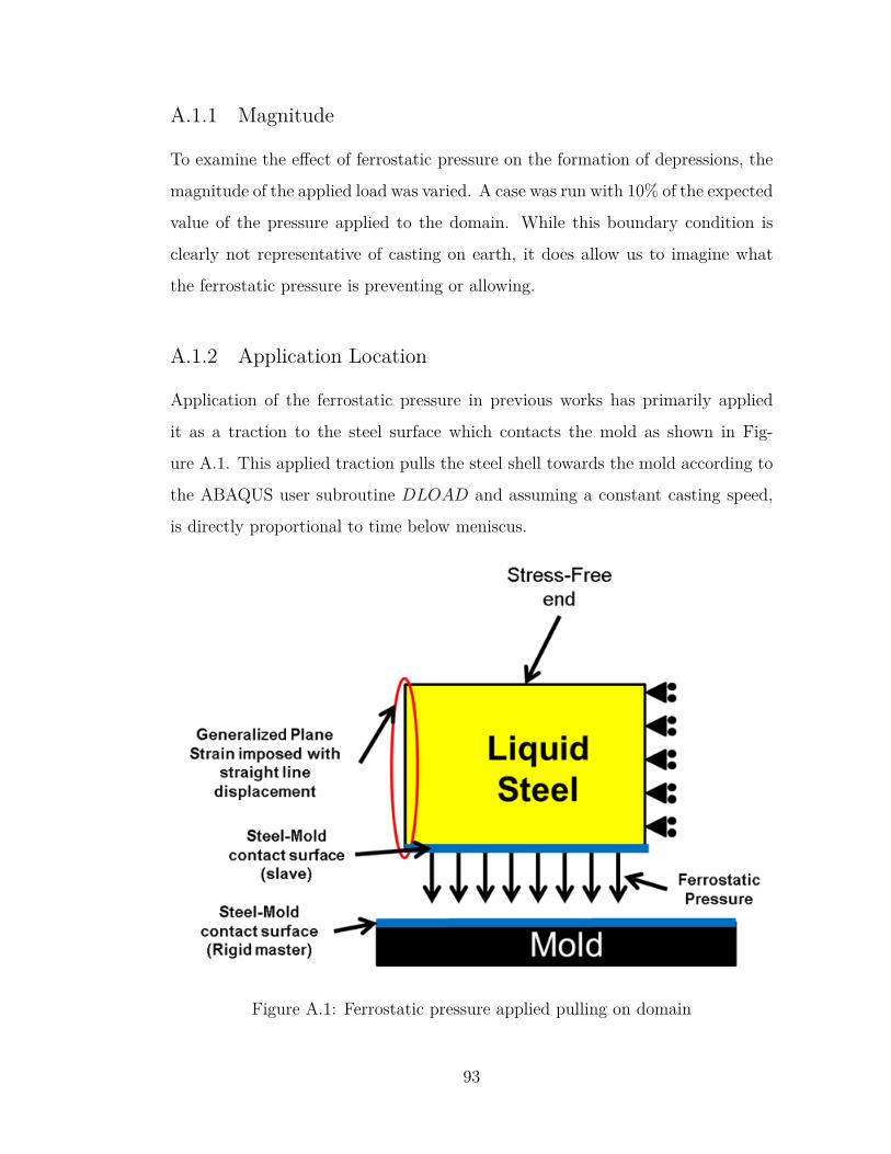
A.1.1 Magnitude

To examine the effect of ferrostatic pressure on the formation of depressions, the

magnitude of the applied load was varied. A case was run with 10% of the expected

value of the pressure applied to the domain. While this boundary condition is

clearly not representative of casting on earth, it does allow us to imagine what

the ferrostatic pressure is preventing or allowing.

A.1.2 Application Location

Application of the ferrostatic pressure in previous works has primarily applied

it as a traction to the steel surface which contacts the mold as shown in Fig-

ure A.1. This applied traction pulls the steel shell towards the mold according to

the ABAQUS user subroutine DLOAD and assuming a constant casting speed,

is directly proportional to time below meniscus.

Figure A.1: Ferrostatic pressure applied pulling on domain

93

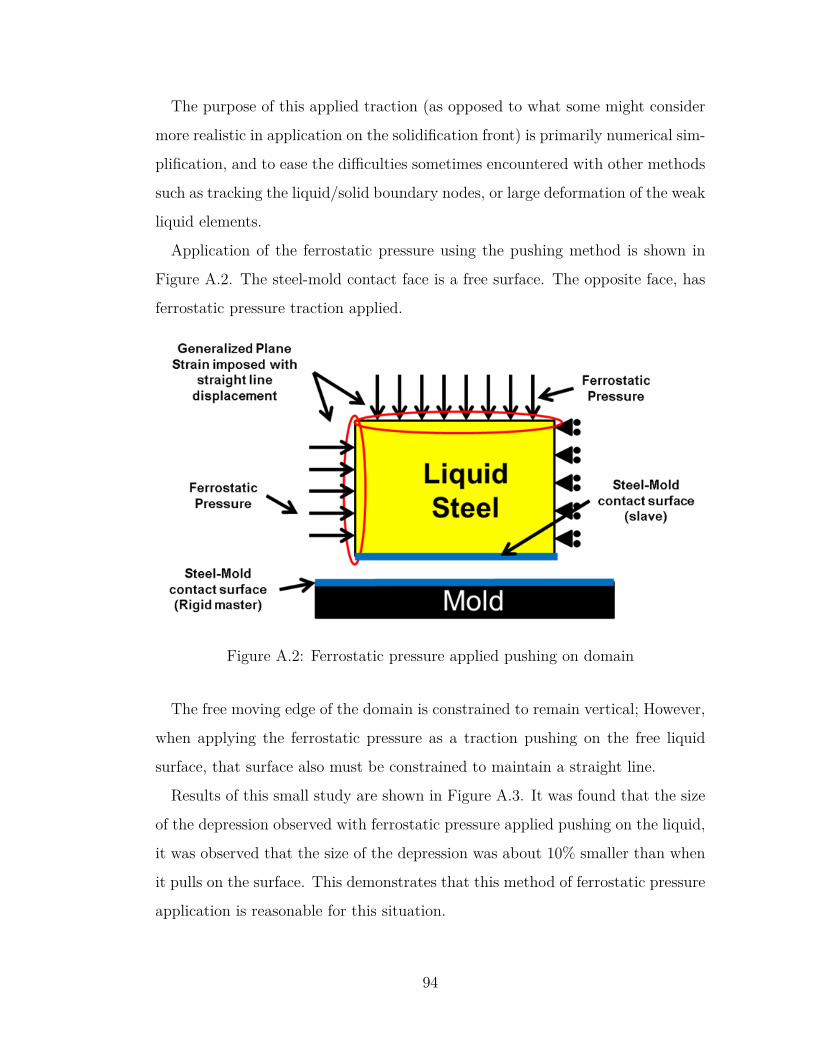
The purpose of this applied traction (as opposed to what some might consider

more realistic in application on the solidification front) is primarily numerical sim-

plification, and to ease the difficulties sometimes encountered with other methods

such as tracking the liquid/solid boundary nodes, or large deformation of the weak

liquid elements.

Application of the ferrostatic pressure using the pushing method is shown in

Figure A.2. The steel-mold contact face is a free surface. The opposite face, has

ferrostatic pressure traction applied.

Figure A.2: Ferrostatic pressure applied pushing on domain

The free moving edge of the domain is constrained to remain vertical; However,

when applying the ferrostatic pressure as a traction pushing on the free liquid

surface, that surface also must be constrained to maintain a straight line.

Results of this small study are shown in Figure A.3. It was found that the size

of the depression observed with ferrostatic pressure applied pushing on the liquid,

it was observed that the size of the depression was about 10% smaller than when

it pulls on the surface. This demonstrates that this method of ferrostatic pressure

application is reasonable for this situation.

94

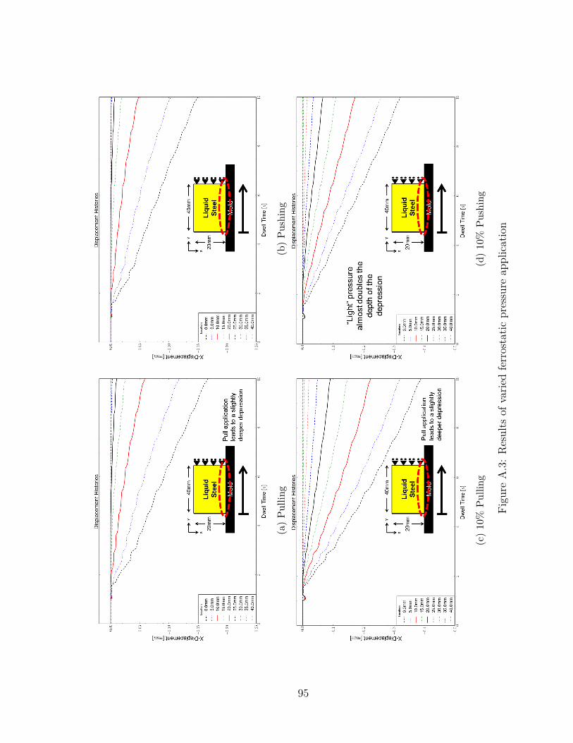
(a)Pu

lling

(b)Pu

shing

(c)10

%Pu

lling

(d)10

%Pu

shing

Figu

reA.3:Results

ofvarie

dferrostatic

pressure

application

95

Appendix B

ABAQUS Operational Notes, Input Files &Scripts

During the course of this work, the author has spent considerable time trou-

bleshooting and exploring solidification modeling using ABAQUS commercial fi-

nite element software. This appendix contains some notes and recommendations

for its successful operations, as well as example input files for the work conducted.

The importance of reading and understanding the documentation cannot be em-

phasized enough, for convenience portions of this chapter contain large excerpts

(some summarized) from the ABAQUS documentation collection.

There is also a section containing the following codes: ABAQUS input files, the

GAPCON subroutine written in FORTRAN, and examples of Python script files

that can be used to run batch jobs for parametric studies, subject to the following

copyright:

Copyright (c) <2016> <Matthew L.S. Zappulla> Permission is hereby granted, free of charge, to any person obtaining

a copy of this software and associated documentation files (the "Software"), to deal in the Software without restriction,

including without limitation the rights to use, copy, modify, merge, publish, distribute, sublicense, and/or sell copies of the

Software, and to permit persons to whom the Software is furnished to do so, subject to the following conditions: The above

copyright notice and this permission notice shall be included in all copies or substantial portions of the Software. THE

SOFTWARE IS PROVIDED "AS IS", WITHOUT WARRANTY OF ANY KIND, EXPRESS OR IMPLIED, INCLUDING

BUT NOT LIMITED TO THE WARRANTIES OF MERCHANTABILITY, FITNESS FOR A PARTICULAR PURPOSE

AND NONINFRINGEMENT. IN NO EVENT SHALL THE AUTHORS OR COPYRIGHT HOLDERS BE LIABLE FOR ANY

CLAIM, DAMAGES OR OTHER LIABILITY, WHETHER IN AN ACTION OF CONTRACT, TORT OR OTHERWISE,

ARISING FROM, OUT OF OR IN CONNECTION WITH THE SOFTWARE OR THE USE OR OTHER DEALINGS IN

THE SOFTWARE.

96

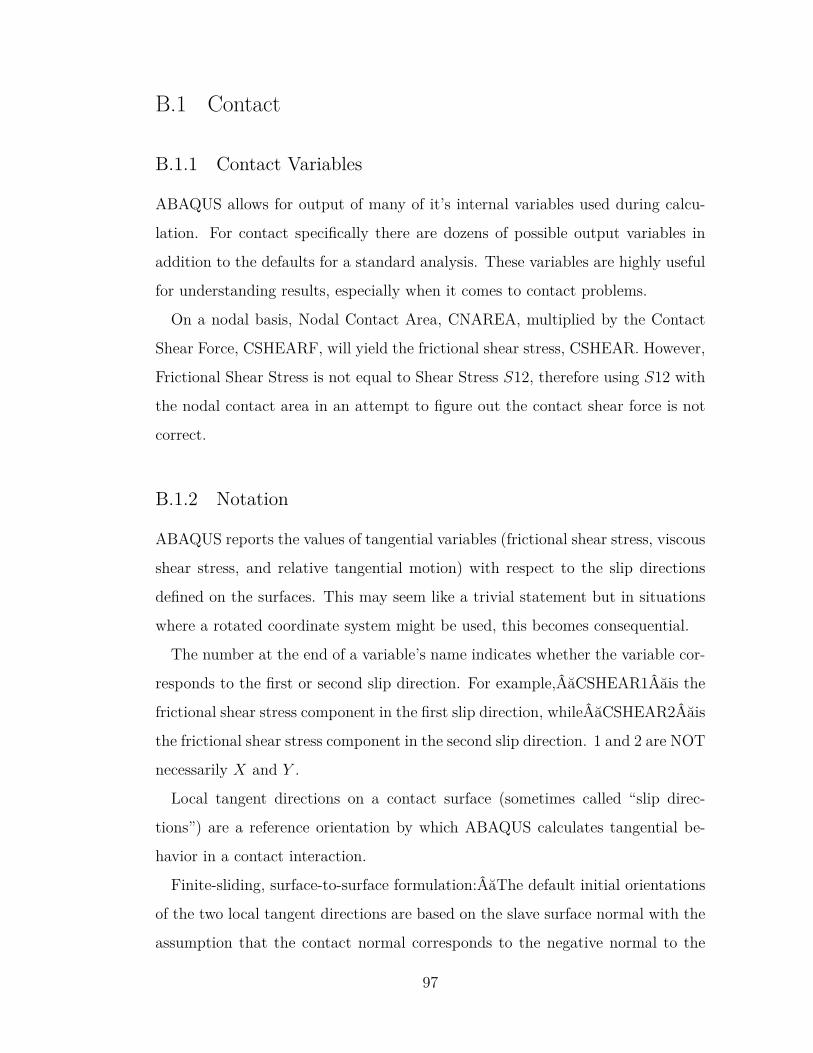
B.1 Contact

B.1.1 Contact Variables

ABAQUS allows for output of many of it’s internal variables used during calcu-

lation. For contact specifically there are dozens of possible output variables in

addition to the defaults for a standard analysis. These variables are highly useful

for understanding results, especially when it comes to contact problems.

On a nodal basis, Nodal Contact Area, CNAREA, multiplied by the Contact

Shear Force, CSHEARF, will yield the frictional shear stress, CSHEAR. However,

Frictional Shear Stress is not equal to Shear Stress S12, therefore using S12 with

the nodal contact area in an attempt to figure out the contact shear force is not

correct.

B.1.2 Notation

ABAQUS reports the values of tangential variables (frictional shear stress, viscous

shear stress, and relative tangential motion) with respect to the slip directions

defined on the surfaces. This may seem like a trivial statement but in situations

where a rotated coordinate system might be used, this becomes consequential.

The number at the end of a variable’s name indicates whether the variable cor-

responds to the first or second slip direction. For example,ÂăCSHEAR1Âăis the

frictional shear stress component in the first slip direction, whileÂăCSHEAR2Âăis

the frictional shear stress component in the second slip direction. 1 and 2 are NOT

necessarily X and Y .

Local tangent directions on a contact surface (sometimes called “slip direc-

tions”) are a reference orientation by which ABAQUS calculates tangential be-

havior in a contact interaction.

Finite-sliding, surface-to-surface formulation:ÂăThe default initial orientations

of the two local tangent directions are based on the slave surface normal with the

assumption that the contact normal corresponds to the negative normal to the

97

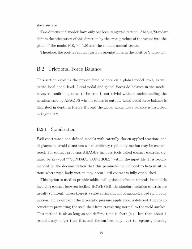
slave surface.

Two-dimensional models have only one local tangent direction. Abaqus/Standard

defines the orientation of this direction by the cross product of the vector into the

plane of the model (0.0, 0.0, 1.0) and the contact normal vector.

Therefore, the positive contact variable orientation is in the positive Y direction.

B.2 Frictional Force Balance

This section explains the proper force balance on a global model level, as well

as the local nodal level. Local nodal and global forces do balance in the model,

however, confirming these to be true is not trivial without understanding the

notation used by ABAQUS when it comes to output. Local nodal force balance is

described in depth in Figure B.1 and the global model force balance is described

in Figure B.2.

B.2.1 Stabilization

Well constrained and defined models with carefully chosen applied tractions and

displacments avoid situations where arbitrary rigid body motion may be encoun-

tered. For contact problems ABAQUS includes tools called contact controls, sig-

nified by keyword “*CONTACT CONTROLS” within the input file. It is recom-

mended by the documentation that this parameter be included to help in situa-

tions where rigid body motion may occur until contact is fully established.

This option is used to provide additional optional solution controls for models

involving contact between bodies. HOWEVER, the standard solution controls are

usually sufficient, unless there is a substantial amount of unconstrained rigid body

motion. For example: if the ferrostatic pressure application is deferred, there is no

constraint preventing the steel shell from translating normal to the mold surface.

This method is ok as long as the defferal time is short (e.g. less than about 1

second), any longer than this, and the surfaces may start to separate, creating

98

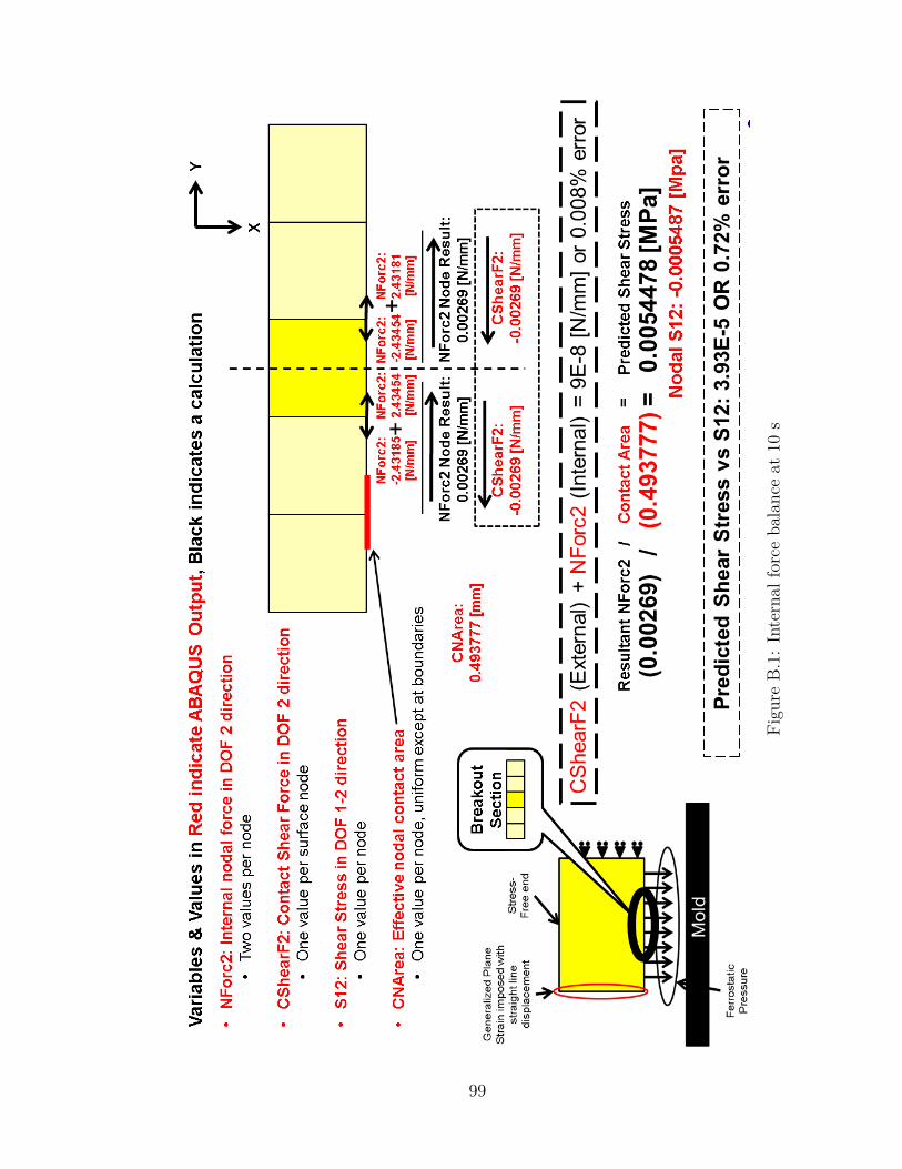
Figu

reB.1:

Internal

forceba

lanceat

10s

99

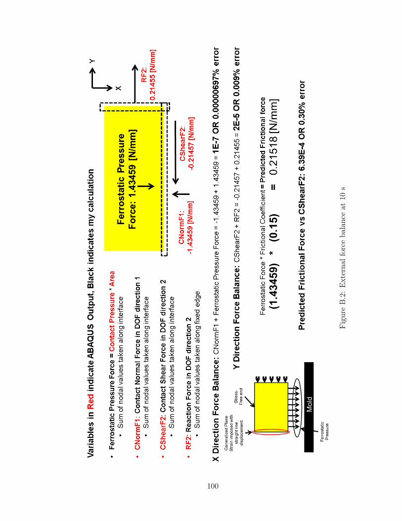
Figu

reB.2:

External

forceba

lanceat

10s

100

not only a non physical situation, but when the traction is finally applied on the

surface, the contact interaction will change abruptly.

It works by activating damping in the normal and tangential directions based

on the stiffness of the underlying mesh and the time step size. If no value is

assigned to this parameter, ABAQUS calculates the damping coefficient auto-

matically. If a numerical value is assigned to this parameter, ABAQUS multiplies

the automatically calculated damping coefficient by this value.

Used improperly this is dangerous In solidification contact problems, this pa-

rameter can be disastrous. For example: Non physical small displacements of

contact surfaces can occur and lead to depression formation in the presence of

completely uniform heat transfer. The lower the amount of stabilization applied

the better.

Heed the warning in the documentation: Warning: These controls are intended

for experienced analysts and should be used with care. Using nondefault values

of these controls may greatly increase the computational time of the analysis or

produce inaccurate results.

Abaqus/Standard offers contact stabilization to help automatically control rigid

body motion in static problems before contact closure and friction restrain such

motion.

It is recommended that you first try to stabilize rigid body motion through

modeling techniques (modifying geometry, imposing boundary conditions, etc.).

The automatic stabilization capability is meant to be used in cases in which it

is clear that contact will be established, but the exact positioning of multiple

bodies is difficult during modeling. It is not meant to simulate general rigid body

dynamics; nor is it meant for contact chattering situations or to resolve initially

tight clearances between mating surfaces.

Although the automatically calculated damping coefficient typically provides

enough damping to eliminate the rigid body modes without having a major effect

on the solution, there is no guarantee that the value is optimal or even suitable.

There are several ways to carry out such checks. The simplest method is to

101

consider the ratio between the energy dissipated by viscous damping and a more

general energy measure for the model, such as the elastic strain energy. These

quantities can be obtained as output variables ALLSD and ALLSE, respectively.

More detailed information can be obtained by comparing the contact damping

stresses CDSTRESS (with the individual components CDPRESS, CDSHEAR1,

and CDSHEAR2) to the true contact stresses CSTRESS (with the individual

components CPRESS, CSHEAR1, and CSHEAR2).

If the contact damping stresses are too high, you should decrease the damping.

The comparison should be made after contact is firmly established; the contact

damping stresses will always be relatively high when contact is not yet or only

partially established.

The easiest way to increase or decrease the amount of damping is to specify

a factor by which the automatically calculated damping coefficient will be mul-

tiplied. Typically, you should initially consider changing the default damping by

(at least) an order of magnitude; if that addresses the problem sufficiently, you

can do some subsequent fine-tuning. In some cases a larger or smaller factor may

be needed; this is not a problem as long as a converged solution is obtained and

the dissipated energy and contact damping stresses are sufficiently small. How-

ever, this is a relative statement, and “sufficiently small” depends directly on the

problem being modeled.

It is also possible to specify the damping coefficient directly. Direct specification

of the damping value is not easy and may require some trial and error.

B.3 Example Input Files

B.3.1 Example Heat Transfer Input Files

**################################################################################*

** #*

** BASIC INPUT FILE TEMPLATE FOR 1D SOLIDIFICATION STRESS PROBLEM #*

102

** #*

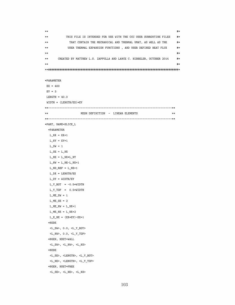
** THIS FILE IS INTENDED FOR USE WITH THE CCC USER SUBROUTINE FILES #*

** THAT CONTAIN THE MECHANICAL AND THERMAL UMAT, AS WELL AS THE #*

** USER THERMAL EXPANSION FUNCTIONS , AND USER DEFINED HEAT FLUX #*

** #*

** CREATED BY MATTHEW L.S. ZAPPULLA AND LANCE C. HIBBELER, OCTOBER 2014 #*

** #*

**################################################################################*

*PARAMETER

EX = 400

EY = 3

LENGTH = 40.0

WIDTH = (LENGTH/EX)*EY

**----------------------------------------------------------------------------**

** MESH DEFINITION - LINEAR ELEMENTS **

**----------------------------------------------------------------------------**

*PART, NAME=SLICE_L

*PARAMETER

L_NX = EX+1

L_NY = EY+1

L_SW = 1

L_SE = L_NX

L_NE = L_NX*L_NY

L_NW = L_NE-L_NX+1

L_ND_REF = L_NE+1

L_DX = LENGTH/EX

L_DY = WIDTH/EY

L_Y_BOT = -0.5*WIDTH

L_Y_TOP = 0.5*WIDTH

L_ME_SW = 1

L_ME_SE = 2

L_ME_NW = L_NX+1

L_ME_NE = L_NX+2

L_E_NE = (EX*EY)-EX+1

*NODE

<L_SW>, 0.0, <L_Y_BOT>

<L_NW>, 0.0, <L_Y_TOP>

*NGEN, NSET=WALL

<L_SW>, <L_NW>, <L_NX>

*NODE

<L_SE>, <LENGTH>, <L_Y_BOT>

<L_NE>, <LENGTH>, <L_Y_TOP>

*NGEN, NSET=FREE

<L_SE>, <L_NE>, <L_NX>

103

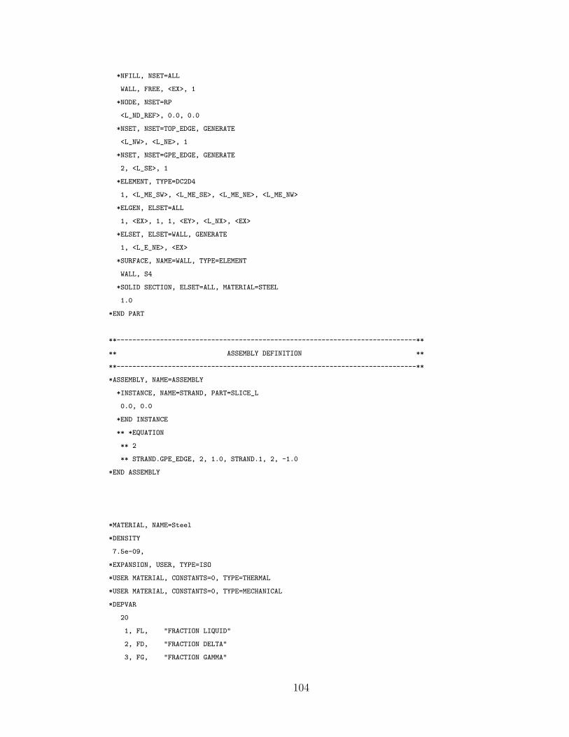
*NFILL, NSET=ALL

WALL, FREE, <EX>, 1

*NODE, NSET=RP

<L_ND_REF>, 0.0, 0.0

*NSET, NSET=TOP_EDGE, GENERATE

<L_NW>, <L_NE>, 1

*NSET, NSET=GPE_EDGE, GENERATE

2, <L_SE>, 1

*ELEMENT, TYPE=DC2D4

1, <L_ME_SW>, <L_ME_SE>, <L_ME_NE>, <L_ME_NW>

*ELGEN, ELSET=ALL

1, <EX>, 1, 1, <EY>, <L_NX>, <EX>

*ELSET, ELSET=WALL, GENERATE

1, <L_E_NE>, <EX>

*SURFACE, NAME=WALL, TYPE=ELEMENT

WALL, S4

*SOLID SECTION, ELSET=ALL, MATERIAL=STEEL

1.0

*END PART

**----------------------------------------------------------------------------**

** ASSEMBLY DEFINITION **

**----------------------------------------------------------------------------**

*ASSEMBLY, NAME=ASSEMBLY

*INSTANCE, NAME=STRAND, PART=SLICE_L

0.0, 0.0

*END INSTANCE

** *EQUATION

** 2

** STRAND.GPE_EDGE, 2, 1.0, STRAND.1, 2, -1.0

*END ASSEMBLY

*MATERIAL, NAME=Steel

*DENSITY

7.5e-09,

*EXPANSION, USER, TYPE=ISO

*USER MATERIAL, CONSTANTS=0, TYPE=THERMAL

*USER MATERIAL, CONSTANTS=0, TYPE=MECHANICAL

*DEPVAR

20

1, FL, "FRACTION LIQUID"

2, FD, "FRACTION DELTA"

3, FG, "FRACTION GAMMA"

104

4, FA, "FRACTION ALPHA"

5, EE11, "ELASTIC STRAIN 11"

6, EE22, "ELASTIC STRAIN 22"

7, EE33, "ELASTIC STRAIN 33"

8, EE12, "ELASTIC STRAIN 12"

9, EEBAR, "EFFECTIVE ELASTIC STRAIN"

10, EP11, "PLASTIC STRAIN 11"

11, EP22, "PLASTIC STRAIN 22"

12, EP33, "PLASTIC STRAIN 33"

13, EP12, "PLASTIC STRAIN 12"

14, EPBAR, "EFFECTIVE PLASTIC STRAIN"

15, EPDOT, "EFFECTIVE PLASTIC STRAIN RATE"

16, EF11, "FLUID STRAIN 11"

17, EF22, "FLUID STRAIN 22"

18, EF33, "FLUID STRAIN 33"

19, EF12, "FLUID STRAIN 12"

20, EFBAR, "EFFECTIVE FLUID STRAIN"

*PHYSICAL CONSTANTS, ABSOLUTE ZERO=-273.15, STEFAN BOLTZMANN=56.704e-09

**

***********************************************************************

** PREDEFINED FIELDS *

***********************************************************************

**

*Initial Conditions, type=TEMPERATURE

STRAND.ALL, 1543.0

*Initial Conditions, type=solution, user

**

**********************************************************************

** STEP DEFINITION *

**********************************************************************

**

*Step, name=ANALYSIS, inc=1000000

*HEAT TRANSFER, DELTMX = 0.5

1e-08, 30.0, 1e-30, 0.01

*CONTROLS, ANALYSIS=DISCONTINUOUS

*CONTROLS, PARAMETERS=TIME INCREMENTATION

10, , ,20,8,5, ,20, , , , ,

0.24,0.4,0.5, , ,0.2, ,

**

**

**************************************************************************

** LOADS *

**************************************************************************

*Dsflux

STRAND.WALL, SNU, 1.0

105

**

**************************************************************************

** OUTPUT *

**************************************************************************

*RESTART, WRITE, OVERLAY, NUMBER INTERVAL=250

*OUTPUT, FIELD, TIME INTERVAL=0.01

*NODE OUTPUT, NSET=STRAND.ALL

NT, UT

*ELEMENT OUTPUT, ELSET=STRAND.ALL

HFL, S, E, THE, EE, SDV

*OUTPUT, DIAGNOSTICS=NO

*END STEP

B.3.2 Example Stress Input Files

**################################################################################*

** #*

** BASIC INPUT FILE TEMPLATE FOR 1D SOLIDIFICATION STRESS PROBLEM #*

** #*

** THIS FILE IS INTENDED FOR USE WITH THE CCC USER SUBROUTINE FILES #*

** THAT CONTAIN THE MECHANICAL AND THERMAL UMAT, AS WELL AS THE #*

** USER THERMAL EXPANSION FUNCTIONS , AND USER DEFINED HEAT FLUX #*

** #*

** CREATED BY MATTHEW L.S. ZAPPULLA AND LANCE C. HIBBELER, OCTOBER 2014 #*

** #*

**################################################################################*

*PARAMETER

EX = 400

EY = 3

LENGTH = 40.0

WIDTH = (LENGTH/EX)*EY

**----------------------------------------------------------------------------**

** MESH DEFINITION - LINEAR ELEMENTS **

**----------------------------------------------------------------------------**

*PART, NAME=SLICE_L

*PARAMETER

L_NX = EX+1

L_NY = EY+1

L_SW = 1

L_SE = L_NX

106

L_NE = L_NX*L_NY

L_NW = L_NE-L_NX+1

L_ND_REF = L_NE+1

L_DX = LENGTH/EX

L_DY = WIDTH/EY

L_Y_BOT = -0.5*WIDTH

L_Y_TOP = 0.5*WIDTH

L_ME_SW = 1

L_ME_SE = 2

L_ME_NW = L_NX+1

L_ME_NE = L_NX+2

L_E_NE = (EX*EY)-EX+1

*NODE

<L_SW>, 0.0, <L_Y_BOT>

<L_NW>, 0.0, <L_Y_TOP>

*NGEN, NSET=WALL

<L_SW>, <L_NW>, <L_NX>

*NODE

<L_SE>, <LENGTH>, <L_Y_BOT>

<L_NE>, <LENGTH>, <L_Y_TOP>

*NGEN, NSET=FREE

<L_SE>, <L_NE>, <L_NX>

*NFILL, NSET=ALL

WALL, FREE, <EX>, 1

*NODE, NSET=RP

<L_ND_REF>, 0.0, 0.0

*NSET, NSET=TOP_EDGE, GENERATE

<L_NW>, <L_NE>, 1

*NSET, NSET=GPE_EDGE, GENERATE

2, <L_SE>, 1

*ELEMENT, TYPE=CPEG4H

1, <L_ME_SW>, <L_ME_SE>, <L_ME_NE>, <L_ME_NW>

*ELGEN, ELSET=ALL

1, <EX>, 1, 1, <EY>, <L_NX>, <EX>

*ELSET, ELSET=WALL, GENERATE

1, <L_E_NE>, <EX>

*SURFACE, NAME=WALL, TYPE=ELEMENT

WALL, S4

*SOLID SECTION, ELSET=ALL, MATERIAL=STEEL, REF NODE=RP

1.0

*END PART

**----------------------------------------------------------------------------**

** ASSEMBLY DEFINITION **

**----------------------------------------------------------------------------**

107

*ASSEMBLY, NAME=ASSEMBLY

*INSTANCE, NAME=STRAND, PART=SLICE_L

0.0, 0.0

*END INSTANCE

*EQUATION

2

STRAND.GPE_EDGE, 2, 1.0, STRAND.1, 2, -1.0

*END ASSEMBLY

*MATERIAL, NAME=Steel

*DENSITY

7.5e-09,

*EXPANSION, USER, TYPE=ISO

*USER MATERIAL, CONSTANTS=0, TYPE=THERMAL

*USER MATERIAL, CONSTANTS=0, TYPE=MECHANICAL

*DEPVAR

20

1, FL, "FRACTION LIQUID"

2, FD, "FRACTION DELTA"

3, FG, "FRACTION GAMMA"

4, FA, "FRACTION ALPHA"

5, EE11, "ELASTIC STRAIN 11"

6, EE22, "ELASTIC STRAIN 22"

7, EE33, "ELASTIC STRAIN 33"

8, EE12, "ELASTIC STRAIN 12"

9, EEBAR, "EFFECTIVE ELASTIC STRAIN"

10, EP11, "PLASTIC STRAIN 11"

11, EP22, "PLASTIC STRAIN 22"

12, EP33, "PLASTIC STRAIN 33"

13, EP12, "PLASTIC STRAIN 12"

14, EPBAR, "EFFECTIVE PLASTIC STRAIN"

15, EPDOT, "EFFECTIVE PLASTIC STRAIN RATE"

16, EF11, "FLUID STRAIN 11"

17, EF22, "FLUID STRAIN 22"

18, EF33, "FLUID STRAIN 33"

19, EF12, "FLUID STRAIN 12"

20, EFBAR, "EFFECTIVE FLUID STRAIN"

*PHYSICAL CONSTANTS, ABSOLUTE ZERO=-273.15, STEFAN BOLTZMANN=56.704e-09

**

***********************************************************************

** PREDEFINED FIELDS *

***********************************************************************

**

*Initial Conditions, type=TEMPERATURE

108

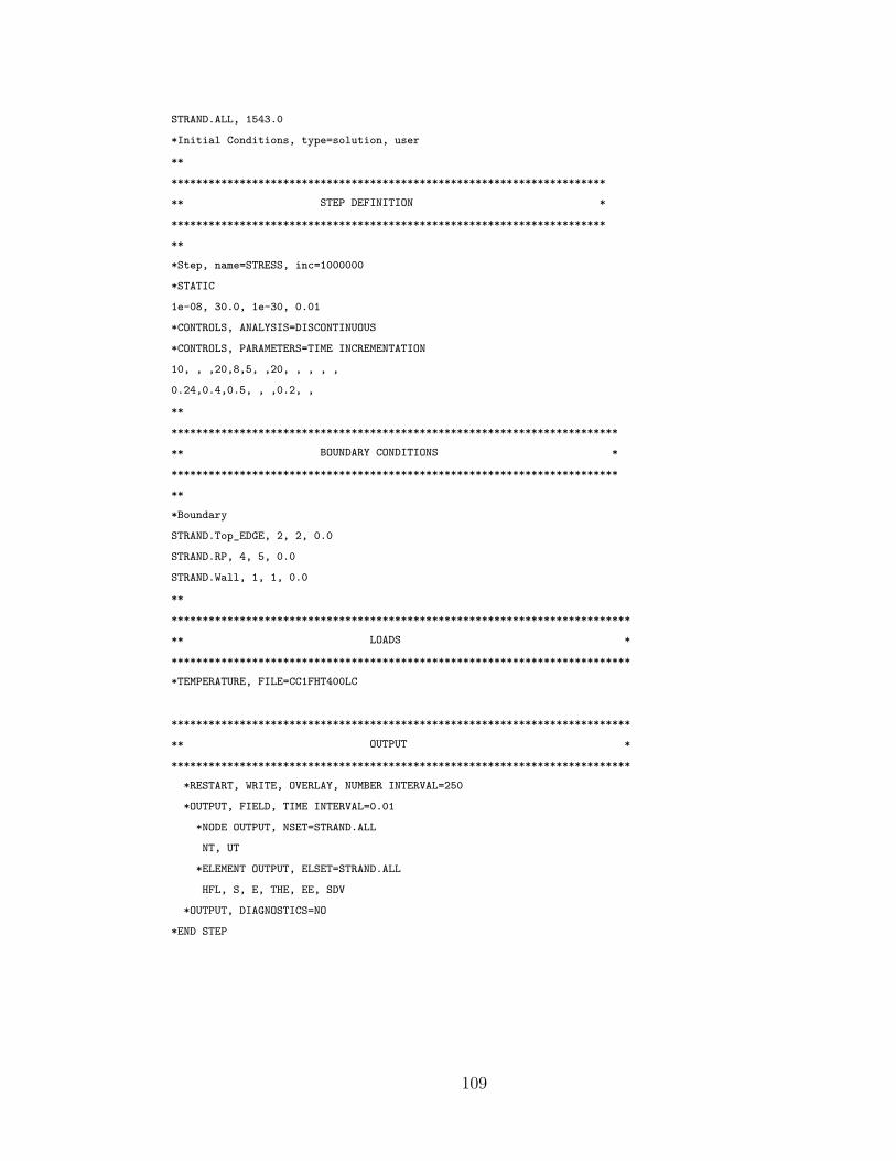
STRAND.ALL, 1543.0

*Initial Conditions, type=solution, user

**

**********************************************************************

** STEP DEFINITION *

**********************************************************************

**

*Step, name=STRESS, inc=1000000

*STATIC

1e-08, 30.0, 1e-30, 0.01

*CONTROLS, ANALYSIS=DISCONTINUOUS

*CONTROLS, PARAMETERS=TIME INCREMENTATION

10, , ,20,8,5, ,20, , , , ,

0.24,0.4,0.5, , ,0.2, ,

**

************************************************************************

** BOUNDARY CONDITIONS *

************************************************************************

**

*Boundary

STRAND.Top_EDGE, 2, 2, 0.0

STRAND.RP, 4, 5, 0.0

STRAND.Wall, 1, 1, 0.0

**

**************************************************************************

** LOADS *

**************************************************************************

*TEMPERATURE, FILE=CC1FHT400LC

**************************************************************************

** OUTPUT *

**************************************************************************

*RESTART, WRITE, OVERLAY, NUMBER INTERVAL=250

*OUTPUT, FIELD, TIME INTERVAL=0.01

*NODE OUTPUT, NSET=STRAND.ALL

NT, UT

*ELEMENT OUTPUT, ELSET=STRAND.ALL

HFL, S, E, THE, EE, SDV

*OUTPUT, DIAGNOSTICS=NO

*END STEP

109

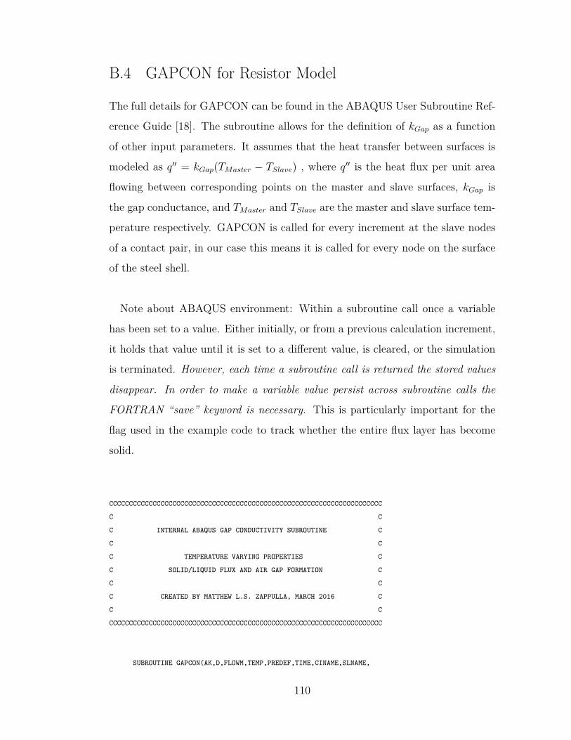
B.4 GAPCON for Resistor Model

The full details for GAPCON can be found in the ABAQUS User Subroutine Ref-

erence Guide [18]. The subroutine allows for the definition of kGap as a function

of other input parameters. It assumes that the heat transfer between surfaces is

modeled as q′′ = kGap(TMaster − TSlave) , where q′′ is the heat flux per unit area

flowing between corresponding points on the master and slave surfaces, kGap is

the gap conductance, and TMaster and TSlave are the master and slave surface tem-

perature respectively. GAPCON is called for every increment at the slave nodes

of a contact pair, in our case this means it is called for every node on the surface

of the steel shell.

Note about ABAQUS environment: Within a subroutine call once a variable

has been set to a value. Either initially, or from a previous calculation increment,

it holds that value until it is set to a different value, is cleared, or the simulation

is terminated. However, each time a subroutine call is returned the stored values

disappear. In order to make a variable value persist across subroutine calls the

FORTRAN “save” keyword is necessary. This is particularly important for the

flag used in the example code to track whether the entire flux layer has become

solid.

CCCCCCCCCCCCCCCCCCCCCCCCCCCCCCCCCCCCCCCCCCCCCCCCCCCCCCCCCCCCCCCCCCCCC

C C

C INTERNAL ABAQUS GAP CONDUCTIVITY SUBROUTINE C

C C

C TEMPERATURE VARYING PROPERTIES C

C SOLID/LIQUID FLUX AND AIR GAP FORMATION C

C C

C CREATED BY MATTHEW L.S. ZAPPULLA, MARCH 2016 C

C C

CCCCCCCCCCCCCCCCCCCCCCCCCCCCCCCCCCCCCCCCCCCCCCCCCCCCCCCCCCCCCCCCCCCCC

SUBROUTINE GAPCON(AK,D,FLOWM,TEMP,PREDEF,TIME,CINAME,SLNAME,

110

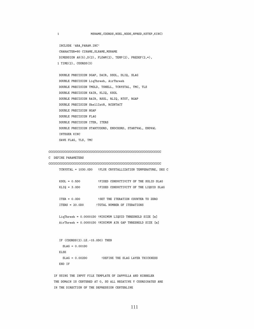
1 MSNAME,COORDS,NOEL,NODE,NPRED,KSTEP,KINC)

INCLUDE ’ABA_PARAM.INC’

CHARACTER*80 CINAME,SLNAME,MSNAME

DIMENSION AK(5),D(2), FLOWM(2), TEMP(2), PREDEF(2,*),

1 TIME(2), COORDS(3)

DOUBLE PRECISION DGAP, DAIR, DSOL, DLIQ, SLAG

DOUBLE PRECISION LiqThresh, AirThresh

DOUBLE PRECISION TMOLD, TSHELL, TCRYSTAL, TMC, TLS

DOUBLE PRECISION KAIR, KLIQ, KSOL

DOUBLE PRECISION RAIR, RSOL, RLIQ, RTOT, RGAP

DOUBLE PRECISION ShellIntR, RCONTACT

DOUBLE PRECISION HGAP

DOUBLE PRECISION FLAG

DOUBLE PRECISION ITER, ITERS

DOUBLE PRECISION STARTCOORD, ENDCOORD, STARTVAL, ENDVAL

INTEGER KINC

SAVE FLAG, TLS, TMC

CCCCCCCCCCCCCCCCCCCCCCCCCCCCCCCCCCCCCCCCCCCCCCCCCCCCCCCCCCCCCCCC

C DEFINE PARAMETERS

CCCCCCCCCCCCCCCCCCCCCCCCCCCCCCCCCCCCCCCCCCCCCCCCCCCCCCCCCCCCCCCC

TCRYSTAL = 1030.0D0 !FLUX CRYSTALLIZATION TEMPERATURE, DEG C

KSOL = 0.5D0 !FIXED CONDUCTIVITY OF THE SOLID SLAG

KLIQ = 3.0D0 !FIXED CONDUCTIVITY OF THE LIQUID SLAG

ITER = 0.0D0 !SET THE ITERATION COUNTER TO ZERO

ITERS = 20.0D0 !TOTAL NUMBER OF ITERATIONS

LiqThresh = 0.00001D0 !MINIMUM LIQUID THRESHOLD SIZE [m]

AirThresh = 0.00001D0 !MINIMUM AIR GAP THRESHOLD SIZE [m]

IF (COORDS(2).LE.-15.0D0) THEN

SLAG = 0.001D0

ELSE

SLAG = 0.002D0 !DEFINE THE SLAG LAYER THICKNESS

END IF

IF USING THE INPUT FILE TEMPLATE OF ZAPPULLA AND HIBBELER

THE DOMAIN IS CENTERED AT 0, SO ALL NEGATIVE Y COORDINATES ARE

IN THE DIRECTION OF THE DEPRESSION CENTERLINE

111

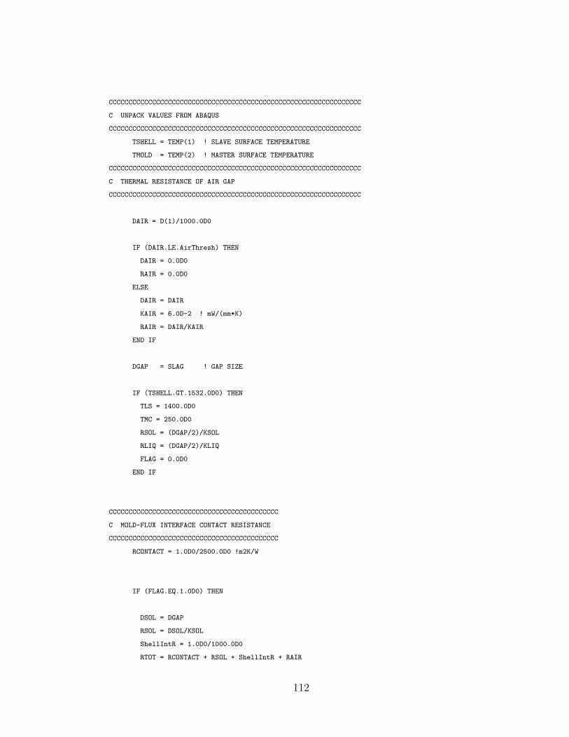
CCCCCCCCCCCCCCCCCCCCCCCCCCCCCCCCCCCCCCCCCCCCCCCCCCCCCCCCCCCCCCCC

C UNPACK VALUES FROM ABAQUS

CCCCCCCCCCCCCCCCCCCCCCCCCCCCCCCCCCCCCCCCCCCCCCCCCCCCCCCCCCCCCCCC

TSHELL = TEMP(1) ! SLAVE SURFACE TEMPERATURE

TMOLD = TEMP(2) ! MASTER SURFACE TEMPERATURE

CCCCCCCCCCCCCCCCCCCCCCCCCCCCCCCCCCCCCCCCCCCCCCCCCCCCCCCCCCCCCCCC

C THERMAL RESISTANCE OF AIR GAP

CCCCCCCCCCCCCCCCCCCCCCCCCCCCCCCCCCCCCCCCCCCCCCCCCCCCCCCCCCCCCCCC

DAIR = D(1)/1000.0D0

IF (DAIR.LE.AirThresh) THEN

DAIR = 0.0D0

RAIR = 0.0D0

ELSE

DAIR = DAIR

KAIR = 6.0D-2 ! mW/(mm*K)

RAIR = DAIR/KAIR

END IF

DGAP = SLAG ! GAP SIZE

IF (TSHELL.GT.1532.0D0) THEN

TLS = 1400.0D0

TMC = 250.0D0

RSOL = (DGAP/2)/KSOL

RLIQ = (DGAP/2)/KLIQ

FLAG = 0.0D0

END IF

CCCCCCCCCCCCCCCCCCCCCCCCCCCCCCCCCCCCCCCCCCC

C MOLD-FLUX INTERFACE CONTACT RESISTANCE

CCCCCCCCCCCCCCCCCCCCCCCCCCCCCCCCCCCCCCCCCCC

RCONTACT = 1.0D0/2500.0D0 !m2K/W

IF (FLAG.EQ.1.0D0) THEN

DSOL = DGAP

RSOL = DSOL/KSOL

ShellIntR = 1.0D0/1000.0D0

RTOT = RCONTACT + RSOL + ShellIntR + RAIR

112

TMC = TMOLD+(TSHELL-TMOLD)*(RCONTACT/RTOT)

TLS = (TMC+(TSHELL-TMOLD)*((RSOL+RAIR)/RTOT))

GOTO 1738

END IF

CCCCCCCCCCCCCCCCCCCCCCCCCCCCCCCCCCCCCCCCCCCCCCCCCCCCCCCCCCCCCCCC

CCCCCCCCCCCCCCCCCCCCCCCCCCCCCCCCCCCCCCCCCCCCCCCCCCCCCCCCCCCCCCCC

C START OF THE GAP LAYER ITERATION LOOP

CCCCCCCCCCCCCCCCCCCCCCCCCCCCCCCCCCCCCCCCCCCCCCCCCCCCCCCCCCCCCCCC

CCCCCCCCCCCCCCCCCCCCCCCCCCCCCCCCCCCCCCCCCCCCCCCCCCCCCCCCCCCCCCCC

DO WHILE(ITER.LT.ITERS)

CCCCCCCCCCCCCCCCCCCCCCCCCCCCCCC

C SHELL INTERFACE RESISTANCE

CCCCCCCCCCCCCCCCCCCCCCCCCCCCCCC

ShellIntR = (3.8981D0*DEXP(0.0054D0*TLS))

IF (ShellIntR.LT.1000.0D0) THEN

ShellIntR = 1000.0D0

END IF

IF (ShellIntR.GT.20000.0D0) THEN

ShellIntR = 20000.0D0

END IF

ShellIntR = 1.0D0/ShellIntR

CCCCCCCCCCCCCCCCCCCCCC

C TOTAL RESISTANCE

CCCCCCCCCCCCCCCCCCCCCC

RTOT = RCONTACT + RLIQ + RSOL + ShellIntR + RAIR

CCCCCCCCCCCCCCCCCCCCCCCCCCCCCCC

C TEMPERATURES THROUGH GAP

CCCCCCCCCCCCCCCCCCCCCCCCCCCCCCCC

TMC = TMOLD+(TSHELL-TMOLD)*(RCONTACT/RTOT)

TLS = (Tmc+(TSHELL-TMOLD)*((RSOL+RLIQ+RAIR)/RTOT))

CCCCCCCCCCCCCCCCCCCCCCCCCCCCCCCCCCCCCCCCCCC

C DIVIDE GAP INTO LIQUID AND SOLID PARTS

CCCCCCCCCCCCCCCCCCCCCCCCCCCCCCCCCCCCCCCCCCCC

DSOL = (TCRYSTAL-TMC)*DGAP/(TLS-TMC)

DLIQ = DGAP-DSOL

113

IF ((DLIQ.LT.LiqThresh).OR.(FLAG.EQ.1.0D0)) THEN

DSOL = DGAP

DLIQ = 0.0D0

RLIQ = 0.0D0

RSOL = DSOL/KSOL

ELSE

RLIQ = DLIQ/KLIQ

RSOL = DSOL/KSOL

END IF

ITER = ITER + 1.0D0

END DO

CCCCCCCCCCCCCCCCCCCCCCCCCCCCCCCCCCCCCCCCCCCCCCCCCCCCCCCCCCCCCCCC

CCCCCCCCCCCCCCCCCCCCCCCCCCCCCCCCCCCCCCCCCCCCCCCCCCCCCCCCCCCCCCCC

C

C END OF THE GAP LAYER ITERATION LOOP

C

CCCCCCCCCCCCCCCCCCCCCCCCCCCCCCCCCCCCCCCCCCCCCCCCCCCCCCCCCCCCCCCC

CCCCCCCCCCCCCCCCCCCCCCCCCCCCCCCCCCCCCCCCCCCCCCCCCCCCCCCCCCCCCCCC

1738 IF ((TSHELL.LT.1400.0D0).AND.(DSOL.EQ.DGAP)) THEN

FLAG = 1.0D0

END IF

CCCCCCCCCCCCCCCCCCCCCCCCCCCCCCCCC

C GAP HEAT TRANSFER COEFFICIENT

CCCCCCCCCCCCCCCCCCCCCCCCCCCCCCCCC

RGAP = RTOT

HGAP = 1.0D0/RGAP

CCCCCCCCCCCCCCCCCCCCCCCCCCCCCCCCCCCC

C PACK VALUES AND RETURN TO ABAQUS

CCCCCCCCCCCCCCCCCCCCCCCCCCCCCCCCCCCC

AK(1) = HGAP/100.0D0 ! GAP CONDUCTANCE, mW/(mm^2*K)

AK(2) = 0.0D0 ! DERIV WRT GAP SIZE

AK(3) = 0.0D0 ! DERIV WRT PRESSURE

AK(4) = 0.0D0 ! DERIV WRT SLAVE SURFACE TEMPERATURE

AK(5) = 0.0D0 ! DERIV WRT MASTER SURFACE TEMPERATURE

RETURN

END SUBROUTINE GAPCON

CCCCCCCCCCCCCCCCCCCCCCCCCCCCCCCCCCCCCCCCCCCCCCCCCCCCCCCCCCCCCCCC

114

CCCCCCCCCCCCCCCCCCCCCCCCCCCCCCCCCCCCCCCCCCCCCCCCCCCCCCCCCCCCCCCC

B.5 Parametric Study Scripts

B.5.1 Discrete Set Parametric Study Script

###################################################################################

# PARAMETRIC STUDY PYTHON SCRIPT #

# WRITTEN BY MATTHEW L.S. ZAPPULLA OCTOBER 7, 2014 #

###################################################################################

Copyright (c) <2016> <Matthew L.S. Zappulla>

###################################################################################

Permission is hereby granted, free of charge, to any person obtaining a copy of

this software and associated documentation files (the "Software"), to deal in the

Software without restriction, including without limitation the rights to use, copy,

modify, merge, publish, distribute, sublicense, and/or sell copies of the Software,

and to permit persons to whom the Software is furnished to do so, subject to the

following conditions:

The above copyright notice and this permission notice shall be included in all copies

or substantial portions of the Software.

THE SOFTWARE IS PROVIDED "AS IS", WITHOUT WARRANTY OF ANY KIND, EXPRESS OR IMPLIED,

INCLUDING BUT NOT LIMITED TO THE WARRANTIES OF MERCHANTABILITY, FITNESS FOR A

PARTICULAR PURPOSE AND NONINFRINGEMENT. IN NO EVENT SHALL THE AUTHORS OR COPYRIGHT

HOLDERS BE LIABLE FOR ANY CLAIM, DAMAGES OR OTHER LIABILITY, WHETHER IN AN ACTION

OF CONTRACT, TORT OR OTHERWISE, ARISING FROM, OUT OF OR IN CONNECTION WITH THE

SOFTWARE OR THE USE OR OTHER DEALINGS IN THE SOFTWARE.

###################################################################################

###################################################################################

# #

# EXECUTE BY GIVING THE COMMAND: ABAQUS SCRIPT=THISFILENAMEWITHOUTEXTENSION #

# #

# BE VERY CAREFUL SETTING UP YOUR INPUT TEMPLATE, COMMENT LINES ARE DANGEROUS #

###################################################################################

# #

# IF NEED BE MULTIPLE CPUS CAN BE SPECIFIED IN THE execOptions area below #

115

# i.e. execOptions=’ USER=umatfile CPUS=numberofcores’ #

# #

###################################################################################

# #

# SETTING UP A MESH PARAMETER PARAMETRIC STUDY #

# #

# MESH STUDIES REQUIRE THAT YOUR MESH GENERATION BE PARAMETER BASED #

# THIS WILL USUALLY REQUIRE NODE GENERATION AND ELEMENT GENERATION #

# #

###################################################################################

# #

# FOR SPECIFIC VALUE EVALUATION (AS OPPOSED TO GENERATING A SAMPLE SET IN A RANGE)#

# parstudyfunction.sample(VALUES, par=parametername, values=(5,11,17,77)) #

# #

# #

# "MESH" KEYWORD WILL CREATE A STUDY FOR ALL POSSIBLE COMBINATIONS #

# #

###################################################################################

## MAIN STUDY SETTINGS

###################################################################################

###################################################################################

#

# THE GENERATED FILES WILL BE: templateinpname_prefix_studyname_C#

# WHERE C# REPRESENTS THE SPECIFIC CASE NUMBER AND IS NOT USER DEFINEABLE

#

# AFTER EXECUTION studyname.var CONTAINS THE DESIGN LIST WITH PARAMETER VALUES

###################################################################################

# THE NAME OF YOUR PARAMETER BASED INPUT FILE OMITTING *.INP

templateinpname = ’BasicTemplate’

# THE PARAMETRIC STUDY NAME, FOLLOWS THE TITLE OF THE TEMPLATE FILE

prefix = ’ParametricStudy’

# THE DESIGN SET NAME, FOLLOWS THE STUDY NAME

studyname = ’DesignSetName’

###################################################################################

# THE NAME OF THE CHANGING PARAMETER IN YOUR INPUT FILE

discparametername = (’EX’, ’MAXSTEP’, ’DELTATEMP’)

# DISCRETE VALUES

discval = ((20, 200, 400, 1000),(0.5, 1.0, 5.0, 10.0),(0.5, 1.0, 10.0, 20.0))

116

###################################################################################

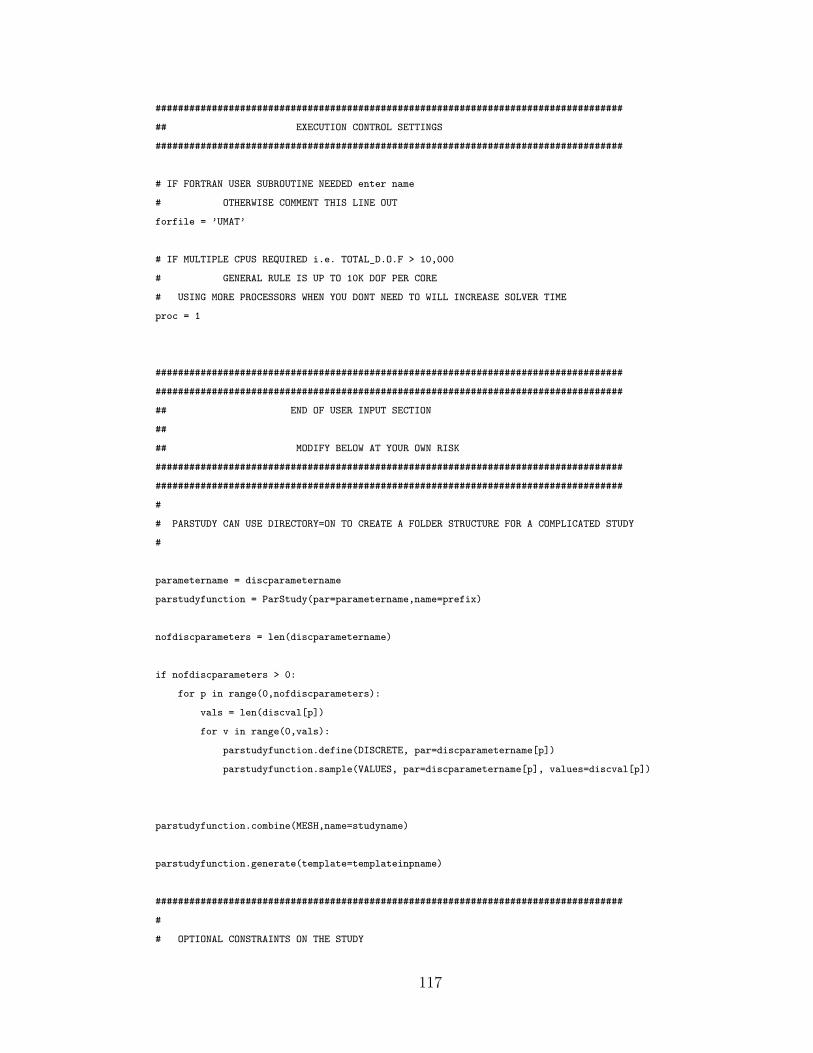
## EXECUTION CONTROL SETTINGS

###################################################################################

# IF FORTRAN USER SUBROUTINE NEEDED enter name

# OTHERWISE COMMENT THIS LINE OUT

forfile = ’UMAT’

# IF MULTIPLE CPUS REQUIRED i.e. TOTAL_D.O.F > 10,000

# GENERAL RULE IS UP TO 10K DOF PER CORE

# USING MORE PROCESSORS WHEN YOU DONT NEED TO WILL INCREASE SOLVER TIME

proc = 1

###################################################################################

###################################################################################

## END OF USER INPUT SECTION

##

## MODIFY BELOW AT YOUR OWN RISK

###################################################################################

###################################################################################

#

# PARSTUDY CAN USE DIRECTORY=ON TO CREATE A FOLDER STRUCTURE FOR A COMPLICATED STUDY

#

parametername = discparametername

parstudyfunction = ParStudy(par=parametername,name=prefix)

nofdiscparameters = len(discparametername)

if nofdiscparameters > 0:

for p in range(0,nofdiscparameters):

vals = len(discval[p])

for v in range(0,vals):

parstudyfunction.define(DISCRETE, par=discparametername[p])

parstudyfunction.sample(VALUES, par=discparametername[p], values=discval[p])

parstudyfunction.combine(MESH,name=studyname)

parstudyfunction.generate(template=templateinpname)

###################################################################################

#

# OPTIONAL CONSTRAINTS ON THE STUDY

117

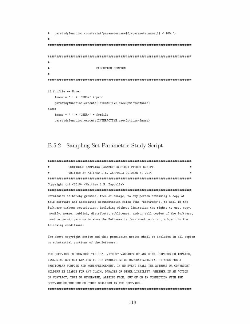
# parstudyfunction.constrain(’parametername[0]*parametername[1] < 100.’)

#

###################################################################################

###################################################################################

#

# EXECUTION SECTION

#

###################################################################################

if forfile == None:

fname = ’ ’ + ’CPUS=’ + proc

parstudyfunction.execute(INTERACTIVE,execOptions=fname)

else:

fname = ’ ’ + ’USER=’ + forfile

parstudyfunction.execute(INTERACTIVE,execOptions=fname)

B.5.2 Sampling Set Parametric Study Script

###################################################################################

# CONTINOUS SAMPLING PARAMETRIC STUDY PYTHON SCRIPT #

# WRITTEN BY MATTHEW L.S. ZAPPULLA OCTOBER 7, 2014 #

###################################################################################

Copyright (c) <2016> <Matthew L.S. Zappulla>

###################################################################################

Permission is hereby granted, free of charge, to any person obtaining a copy of

this software and associated documentation files (the "Software"), to deal in the

Software without restriction, including without limitation the rights to use, copy,

modify, merge, publish, distribute, sublicense, and/or sell copies of the Software,

and to permit persons to whom the Software is furnished to do so, subject to the

following conditions:

The above copyright notice and this permission notice shall be included in all copies

or substantial portions of the Software.

THE SOFTWARE IS PROVIDED "AS IS", WITHOUT WARRANTY OF ANY KIND, EXPRESS OR IMPLIED,

INCLUDING BUT NOT LIMITED TO THE WARRANTIES OF MERCHANTABILITY, FITNESS FOR A

PARTICULAR PURPOSE AND NONINFRINGEMENT. IN NO EVENT SHALL THE AUTHORS OR COPYRIGHT

HOLDERS BE LIABLE FOR ANY CLAIM, DAMAGES OR OTHER LIABILITY, WHETHER IN AN ACTION

OF CONTRACT, TORT OR OTHERWISE, ARISING FROM, OUT OF OR IN CONNECTION WITH THE

SOFTWARE OR THE USE OR OTHER DEALINGS IN THE SOFTWARE.

###################################################################################

118

###################################################################################

# #

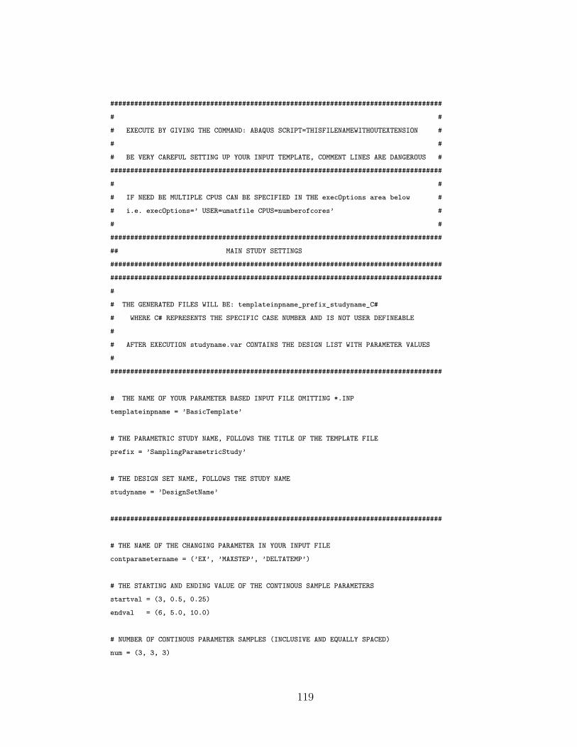
# EXECUTE BY GIVING THE COMMAND: ABAQUS SCRIPT=THISFILENAMEWITHOUTEXTENSION #

# #

# BE VERY CAREFUL SETTING UP YOUR INPUT TEMPLATE, COMMENT LINES ARE DANGEROUS #

###################################################################################

# #

# IF NEED BE MULTIPLE CPUS CAN BE SPECIFIED IN THE execOptions area below #

# i.e. execOptions=’ USER=umatfile CPUS=numberofcores’ #

# #

###################################################################################

## MAIN STUDY SETTINGS

###################################################################################

###################################################################################

#

# THE GENERATED FILES WILL BE: templateinpname_prefix_studyname_C#

# WHERE C# REPRESENTS THE SPECIFIC CASE NUMBER AND IS NOT USER DEFINEABLE

#

# AFTER EXECUTION studyname.var CONTAINS THE DESIGN LIST WITH PARAMETER VALUES

#

###################################################################################

# THE NAME OF YOUR PARAMETER BASED INPUT FILE OMITTING *.INP

templateinpname = ’BasicTemplate’

# THE PARAMETRIC STUDY NAME, FOLLOWS THE TITLE OF THE TEMPLATE FILE

prefix = ’SamplingParametricStudy’

# THE DESIGN SET NAME, FOLLOWS THE STUDY NAME

studyname = ’DesignSetName’

###################################################################################

# THE NAME OF THE CHANGING PARAMETER IN YOUR INPUT FILE

contparametername = (’EX’, ’MAXSTEP’, ’DELTATEMP’)

# THE STARTING AND ENDING VALUE OF THE CONTINOUS SAMPLE PARAMETERS

startval = (3, 0.5, 0.25)

endval = (6, 5.0, 10.0)

# NUMBER OF CONTINOUS PARAMETER SAMPLES (INCLUSIVE AND EQUALLY SPACED)

num = (3, 3, 3)

119

###################################################################################

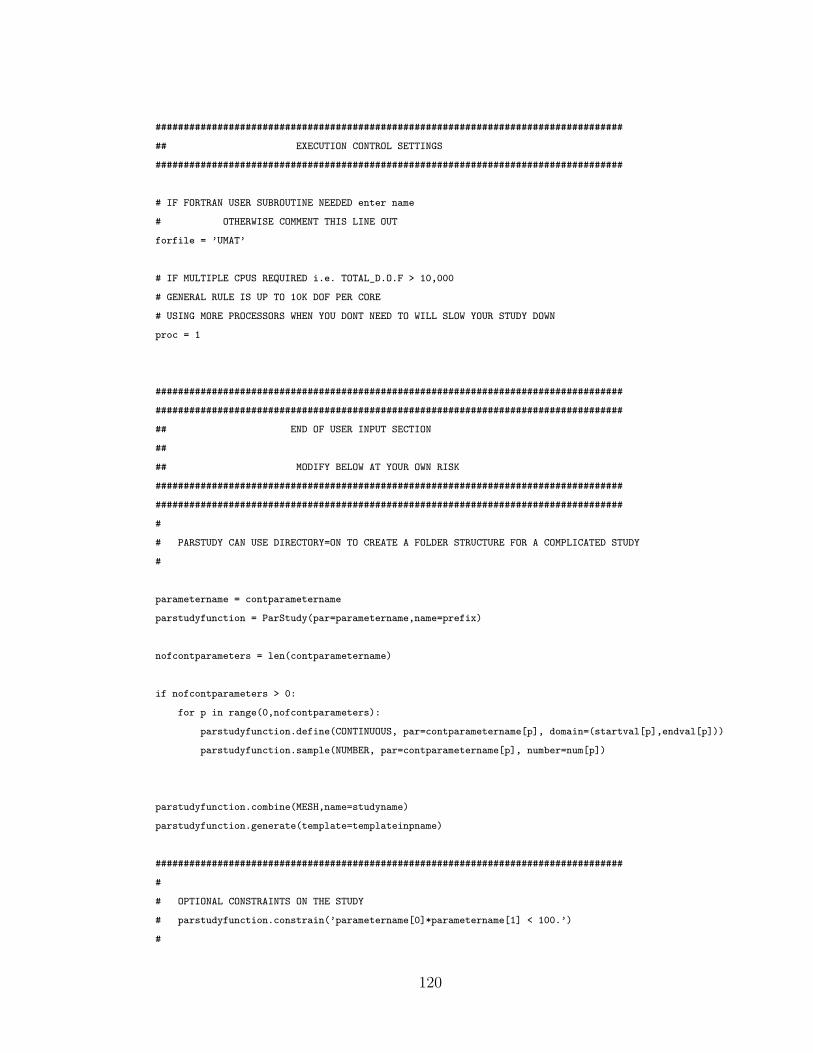
## EXECUTION CONTROL SETTINGS

###################################################################################

# IF FORTRAN USER SUBROUTINE NEEDED enter name

# OTHERWISE COMMENT THIS LINE OUT

forfile = ’UMAT’

# IF MULTIPLE CPUS REQUIRED i.e. TOTAL_D.O.F > 10,000

# GENERAL RULE IS UP TO 10K DOF PER CORE

# USING MORE PROCESSORS WHEN YOU DONT NEED TO WILL SLOW YOUR STUDY DOWN

proc = 1

###################################################################################

###################################################################################

## END OF USER INPUT SECTION

##

## MODIFY BELOW AT YOUR OWN RISK

###################################################################################

###################################################################################

#

# PARSTUDY CAN USE DIRECTORY=ON TO CREATE A FOLDER STRUCTURE FOR A COMPLICATED STUDY

#

parametername = contparametername

parstudyfunction = ParStudy(par=parametername,name=prefix)

nofcontparameters = len(contparametername)

if nofcontparameters > 0:

for p in range(0,nofcontparameters):

parstudyfunction.define(CONTINUOUS, par=contparametername[p], domain=(startval[p],endval[p]))

parstudyfunction.sample(NUMBER, par=contparametername[p], number=num[p])

parstudyfunction.combine(MESH,name=studyname)

parstudyfunction.generate(template=templateinpname)

###################################################################################

#

# OPTIONAL CONSTRAINTS ON THE STUDY

# parstudyfunction.constrain(’parametername[0]*parametername[1] < 100.’)

#

120

###################################################################################

###################################################################################

#

# EXECUTION SECTION

#

###################################################################################

if forfile == None:

fname = ’ ’ + ’CPUS=’ + proc

parstudyfunction.execute(INTERACTIVE,execOptions=fname)

else:

fname = ’ ’ + ’USER=’ + forfile

parstudyfunction.execute(INTERACTIVE,execOptions=fname)

121

References

[1] J. S. Spoerl, “A Brief History of Iron and Steel Production.”http://www.anselm.edu/homepage/dbanach/h-carnegie-steel.htm, 2013.

[2] H. Bessemer, “The Bessemer Steel Works At Troy,” The Journal of TheFranklin Institute, pp. 82–83, 1845.

[3] S. Mizoguchi, T. Ohashi, and T. Saeki, “Continuous Casting of Steel,” An-nual Review Material Science, pp. 151–169, 1981.

[4] J. Elfsberg, Oscillation Mark Formation in Continuous Casting Processes.PhD thesis, Royal Institute of Technology, 2003.

[5] E. Studies, “Steel Statistical Yearbook,” Steel Statistical Yearbook 2014worldsteel, vol. 1, p. 121, 2011.

[6] H. Bessemer, “Improvement in the manufacture of iron and steel.” U.S.Patent: US49053 A, 1865.

[7] B. G. Thomas, “Introduction to Continuous Casting.”http://ccc.mechse.uiuc.edu/introduction/concast.html.

[8] A. W. Cramb, “High Purity , Low Residual and Clean Steels.”

[9] J. Oda, K. Akimoto, and T. Tomoda, “Long-term global availability of steelscrap,” Resources, Conservation and Recycling, vol. 81, pp. 81–91, 2013.

[10] A. W. Cramb, “Issues in Caster Operation.” Brimacombe Continuous Cast-ing Course-Vancouver, 2013.

[11] I. V. Samarasekera and C. Chow, “Continuous Casting of Steel Billets,” inMaking, Shaping and Treating of Steel, ch. 18, pp. 1–46, Pittsburgh, PA:AISE Steel Foundation, 11th ed., 2002.

[12] A. W. Cramb, R. Rastogi, and R. L. Maddalena, “Nozzle Clogging,” inMaking, Shaping and Treating of Steel, ch. 10, pp. 1–17, Pittsburgh, PA:AISE Steel Foundation, 2002.

122

[13] L. C. Hibbeler and B. G. Thomas, “Mold Slag Entrainment Mechanisms inContinuous Casting Molds,” in AISTech - Iron and Steel Technology Con-ference Proceedings, pp. 1215–1230, 2013.

[14] AEIS, “Effects of alloying elements on Steel.”http://www.aeisndt.com/pdf/1 Effects of Alloying Elements on Steel.pdf,2010.

[15] Z. G. Yang, D. M. Paxton, K. S. Weil, J. W. Stevenson, and P. Singh, “Ma-terials Properties Database for Selection of High-Temperature Alloys andConcepts of Alloy Design for SOFC Applications,” Tech. Rep. November,Pacific Northwest National Laboratory, Richland, Washington, 2002.

[16] J. K. Brimacombe and K. Sorimachi, “Crack formation in the continuouscasting of steel,” Metallurgical and Materials Transactions B, vol. 8, no. 2,pp. 489–505, 1977.

[17] S. Watanabe, K. Harada, and F. HitoshiShiro, “Continuous Casting,” Tetsu-to-Hagané, vol. 58, no. 11, p. S393, 1972.

[18] Simulia, Analysis User’ s Manual: User Subroutines and Parametric Studies,vol. VI. DS SIMULIA Corp, 2011.

[19] S. Koric, Efficient Thermo-Mechanical Model for Solidification Processesand its Applications in Steel Continuous Casting. PhD thesis, The Univer-sity of Illinois at Urbana-Champaign, 2006.

[20] Y. Ueshima, S. Mizoguchi, T. Matsumiya, and H. Kajioka, “Analysis of so-lute distribution in dendrites of carbon steel with δ/γ transformation duringsolidification,” Metallurgical and Materials Transactions B, vol. 17, no. 4,pp. 845–859, 1986.

[21] J. D. Hunt, “Steady state columnar and equiaxed growth of dendrites andeutectic,” Materials Science and Engineering, vol. 65, no. 1, pp. 75–83, 1984.

[22] W. Kurz, “About initial solidification in continuous casting of steel,” Met-allurgia Italiana, vol. 100, no. 7, pp. 56–64, 2008.

[23] W. Kurz and D. J. Fisher, “Dendrite growth at the limit of stability: tipradius and spacing,” Acta Metallurgica, vol. 29, no. 1, pp. 11–20, 1981.

[24] J. Lipton, W. Kurz, and R. Trivedi, “Rapid dendrite growth in undercooledalloys,” Acta Metallurgica, vol. 35, no. 4, pp. 957–964, 1987.

[25] A. Chojecki, I. Telejko, and T. Bogacz, “Influence of chemical compositionon the hot tearing formation of cast steel,” Theoretical and Applied FractureMechanics, vol. 27, no. 2, pp. 99–105, 1997.

123

[26] W. T. Lankford, “Some considerations of strength and ductility in thecontinuous-casting process,” Metallurgical Transactions, vol. 3, no. 6,pp. 1331–1357, 1972.

[27] J. Miettinen, S. Louhenkilpi, H. Kytönen, and J. Laine, “IDS: Thermo-dynamic kinetic empirical tool for modelling of solidification, microstruc-ture and material properties,” Mathematics and Computers in Simulation,vol. 80, no. 7, pp. 1536–1550, 2010.

[28] Y. M. Won, K.-h. Kim, T.-j. Yeo, and K. H. Oh, “Effect of Cooling Rateon ZST, LIT and ZDT of Carbon Steels Near Melting Point,” ISIJ Inter-national, vol. 38, no. 10, pp. 1093–1099, 1998.

[29] K.-h. Kim, T.-j. Yeo, K. H. Oh, and D. N. Lee, “Effect of Carbon andSulfur in Continuously Cast Strand on Longitudinal Surface Cracks,” ISIJInternational, vol. 36, no. 3, pp. 284–289, 1996.

[30] K. E. Blazek, O. Lanzi, P. L. Gano, and D. L. Kellogg, “Calculation of theperitectic range for steel alloys,” in AISTech - Iron and Steel TechnologyConference Proceedings, vol. 5, pp. 80–85, 2008.

[31] M. H. Burden and J. D. Hunt, “A Mechanism for the Columnar to EquiaxedTransition in Castings or Ingots,” Metallurgical and Materials TransactionsA, vol. 6A, pp. 240–241, 1975.

[32] S. C. Flood and J. D. Hunt, “Columnar and equiaxed growth. II. Equiaxedgrowth ahead of a columnar front,” Journal of Crystal Growth, vol. 82, no. 3,pp. 552–560, 1987.

[33] W. J. Poole and F. Weinberg, “Observations of the columnar-to-equiaxedtransition in stainless steels,” Metallurgical and Materials Transactions A,vol. 29, no. 3, pp. 855–861, 1998.

[34] M. Rappaz, J. Drezet, and M. Gremaud, “A New Hot-Tearing Criterion,”Metallurgical and Materials Transactions A, vol. 30A, pp. 449–455, 1999.

[35] Y. M. Won, T.-j. Yeo, D. J. Seol, and K. H. Oh, “A new criterion for internalcrack formation in continuously cast steels,” Metallurgical and MaterialsTransactions B, vol. 31, no. 4, pp. 779–794, 2000.

[36] D. G. Eskin and L. Katgerman, “Mechanical properties in the semi-solidstate and hot tearing of aluminium alloys,” Progress in Materials Science,vol. 49, pp. 629–711, 2004.

[37] T. W. Clyne and G. J. Davies, “The influence of composition on solidifica-tion cracking susceptibility in binary alloy systems,” British Foundryman,vol. 74, pp. 65–73, 1981.

124

[38] H. Mizukami, S. Hiraki, M. Kawamoto, and T. Watanabe, “Initial Solidifi-cation Behavior of Ultra Low, Low and Middle Carbon Steel.,” ISIJ Inter-national, vol. 39, no. 12, pp. 1262–1269, 1999.

[39] M. M. Wolf and K. Kurz, “The Effect of Carbon Content on Solidifica-tion of Steel in the Continuous Casting Mold,” Metallurgical and MaterialsTransactions B, vol. 12, no. 1, pp. 85–93, 1981.

[40] M. Suzuki and Y. Yamaoka, “Influence of Carbon Content on SolidifyingShell Growth of Carbon Steels at the Initial Stage of Solidification,” Mate-rials Transactions, vol. 44, no. 5, pp. 836–844, 2003.

[41] B. Thomas and C. Ojeda, “Ideal taper prediction for slab casting,” in ISSSteelmaking Conference, (Indianapolis, IN), pp. 295–308, ISS-AIME, 2003.

[42] H. Mehrara, D. G. Eskin, R. H. Petrov, M. Lalpoor, and L. Katgerman,“Linear contraction behavior of low-carbon, low-alloy steels during and aftersolidification using real-time measurements,” Metallurgical and MaterialsTransactions A, vol. 45, no. 3, pp. 1445–1456, 2014.

[43] M. Reid, D. Phelan, and R. J. Dippenaar, “Concentric Solidification forHigh Temperature Laser Scanning Confocal Microscopy,” ISIJ Interna-tional, vol. 44, no. 3, pp. 565–572, 2004.

[44] M. Rowan, B. G. Thomas, R. Pierer, and C. Bernhard, “Measuring me-chanical behavior of steel during solidification: Modeling the SSCC test,”Metallurgical and Materials Transactions B, vol. 42, no. 4, pp. 837–851,2011.

[45] A. Lagerstedt and H. Fredriksson, “A model for prediction of cracks in asolidifying shell,” Materials Science and Engineering: A, vol. 414, pp. 37–43,2005.

[46] Y. Meng, C. Li, J. Parkman, and B. G. Thomas, “Simulation of shrinkageand stress in solidifying steel shells of different grades,” in InternationalConference on Modeling of Casting, Welding and Advanced SolidificationProcesses (M. Rappaz, ed.), (Charlotte, NC), pp. 33–39, The Minerals, Met-als & Materials Society, 2004.

[47] H. G. Suzuki, S. Nishimura, and S. Yamaguchi, “Characteristics of HotDuctility in Steels Subjected to the Melting and Solidification,” Transactionsof the Iron and Steel Institute of Japan, vol. 22, no. 1, pp. 48–56, 1982.

[48] P. J. Wray, “Tensile Failure Behavior of Plain Carbon Steels at ElevatedTemperatures,” Metallurgical and Materials Transactions A, vol. 15, no. 11,pp. 2059–2073, 1984.

125

[49] B. G. Thomas, J. K. Brimacombe, and I. V. Samarasekera, “The Formationof Panel Cracks in Steel Ingots: A State-of-the-Art Review, I. Hot Ductilityof Steel,” Transactions of the Iron and Steel Society, vol. 7, no. 10, pp. 7–20,1986.

[50] C. H. Yu, M. Suzuki, H. Shibata, and T. Emi, “Simulation of Crack Forma-tion on Solidifying Steel Shell in Continuous Casting Mold.,” ISIJ Interna-tional, vol. 36, no. Suppl, pp. S159–S162, 1996.

[51] M. B. Santillana, Thermo-mechanical properties and cracking during solid-ification of thin slab cast steel. PhD thesis, Delft University of Technology,2013.

[52] S. Singh and K. E. Blazek, “Heat transfer and skin formation in acontinuous-casting mold as a function of steel carbon content,” Journal ofMetals, pp. 17–27, 1974.

[53] S. Moon, The peritectic phase transition and continuous casting practice.PhD thesis, University of Wollongong, 2015.

[54] J. Konishi, M. Militzer, I. V. Samarasekera, and J. K. Brimacombe, “Mod-eling the formation of longitudinal facial cracks during continuous casting ofhypoperitectic steel,” Metallurgical and Materials Transactions B, vol. 33B,pp. 413–423, 2002.

[55] P. Presoly, R. Pierer, and C. Bernhard, “Identification of defect prone peri-tectic steel grades by analyzing high-temperature phase transformations,”Metallurgical and Materials Transactions A, vol. 44, no. 12, pp. 5377–5388,2013.

[56] E. Wielgosz and T. Kargul, “Differential scanning calorimetry study of peri-tectic steel grades,” Journal of Thermal Analysis and Calorimetry, vol. 119,no. 3, pp. 1547–1553, 2015.

[57] A. Kagawa and T. Okamoto, “Influence of alloying elements on temperatureand composition for peritectic reaction in plain carbon steels,” MaterialsScience and Technology, vol. 2, no. 10, pp. 997–1008, 1986.

[58] C. Bale, P. Chartrand, and S. Degterov, “FactSage thermochemical softwareand databases,” 2002.

[59] N. Saunders, U. K. Z. Guo, X. Li, a. P. Miodownik, and J. P. Schillé, “UsingJMatPro to model materials properties and behavior,” The Journal of TheMinerals, Metals & Materials Society (TMS), vol. 55, pp. 60–65, 2003.

[60] J. O. Andersson, T. Helander, L. Hoglund, P. Shi, and B. Sundman,“THERMO-CALC & DICTRA, Computational Tools For Materials Sci-ence,” Calphad, vol. 26, no. 2, pp. 273–312, 2002.

126

[61] R. D. Pehlke, R. D. Jeyarajan, and H. Wada, “Summary of Thermal Prop-erties for Casting Alloys and Mold Materials,” tech. rep., National ScienceFoundation: Applied Research Division, Ann Arbor, Michigan, 1982.

[62] A. Jablonka, K. Harste, and K. Schwerdtfeger, “Thermomechanical proper-ties of iron and iron-carbon alloys: density and thermal contraction,” Steelresearch, vol. 62, no. 1, pp. 24–33, 1991.

[63] P. J. Wray, “High Temperature Plastic-Flow Behavior of Mixtures ofAustenite, Cementite, Ferrite, and Pearlite in Plain-Carbon Steels,” Met-allurgical and Materials Transactions A, vol. 15A, no. 11, pp. 2041–2058,1984.

[64] C. Li and B. G. Thomas, “Thermomechanical finite-element model of shellbehavior in continuous casting of steel,” Metallurgical and Materials Trans-actions B, vol. 35, no. 6, pp. 1151–1172, 2004.

[65] J. Sengupta, C. Ojeda, and B. G. Thomas, “Thermal-mechanical behaviourduring initial solidification in continuous casting: steel grade effects,” Inter-national Journal of Cast Metals Research, vol. 22, no. 1, pp. 8–14, 2009.

[66] B. G. Thomas, G. Li, A. Moitra, and D. Habing, “Analysis of Thermal andMechanical Behavior of Copper Molds during Continuous Casting of SteelSlabs,” in 80th Steelmaking Conference, (Chicago, Illinois), pp. 1–19, 1997.

[67] R. J. Dippenaar, I. V. Samarasekera, and J. K. Brimacombe, “Mold taperin continuous casting billet machines,” ISS Transactions, vol. 7, pp. 33–43,1986.

[68] D. P. Lorento, “Billet Mold Taper and Secondary Cooling Pattern Design.”Private Communication, 2002.

[69] C. Li and B. G. Thomas, “Maximum casting speed for continuous cast steelbillets based on sub-mold bulging computation,” in 85th Steelmaking Con-ference Proceedings, (Warrendale, PA), pp. 109–130, Iron and Steel Society,2002.

[70] C. Li and B. G. Thomas, “Ideal taper prediction for billet casting,” ISSSteelmaking Conference, pp. 295–308, 2003.

[71] Ridolfi, B. G. Thomas, and Foglia, “The optimization of mold taper for theIlva-Dalmine round bloom caster,” La Revue de Metallurgie-CIT, vol. 91,no. 4, pp. 609–620, 1994.

[72] B. G. Thomas and W. Storkman, “Mathematical Models of Continuous SlabCasting to Optimize Mold Taper,” in Modeling and Control of Casting andWelding Processes - IV (A. Giamei and G. Abbaschian, eds.), (Palm Coast,Florida), pp. 287–297, The Metallurgical Society, 1988.

127

[73] A. Moitra, B. G. Thomas, and W. Storkman, “Thermo-Mechanical Modelof Steel Shell Behavior in the Continuous Casting Mold,” in TMS AnnualMeeting, (San Diego, CA), pp. 1–31, The Minerals, Metals & MaterialsSociety, 1992.

[74] B. Bottger, M. Apel, M. B. Santillana, and D. G. Eskin, “Relationship be-tween solidification microstructure and hot cracking susceptibility for con-tinuous casting of low-carbon and high-strength low-alloyed steels: A phase-field study,” Metallurgical and Materials Transactions A, vol. 44, no. 8,pp. 3765–3777, 2013.

[75] J. Tiaden, “Phase field simulations of the peritectic solidification of Fe-C,”Journal of Crystal Growth, vol. 198-199, pp. 1275–1280, 1999.

[76] B. Bottger, G. J. Schmitz, and M. B. Santillana, “Multi-phase-field mod-eling of solidification in technical steel grades,” Transactions of the IndianInstitute of Metals, vol. 65, no. 6, pp. 613–615, 2012.

[77] B. G. Thomas, G. Li, A. Moitra, and D. Habing, “Analysis of thermaland mechanical behavior of copper molds during continuous casting of steelslabs,” Iron and Steelmaker(USA), pp. 1–19, 1998.

[78] A. Howe, “Micro-Segregation: Issues of Growth Rate and the Peritectic,”Materials Science Forum, vol. 649, pp. 419–424, 2010.

[79] H. Fredriksson, “The mechanism of the peritectic reaction in iron-base al-loys,” Metal Science, vol. 10, no. 3, pp. 77–86, 1976.

[80] H. Mizukami, A. Yamanaka, and T. Watanabe, “Prediction of Density ofCarbon Steels.,” ISIJ International, vol. 42, no. 4, pp. 375–384, 2002.

[81] M. L. S. Zappulla, L. C. Hibbeler, and B. G. Thomas, “Thermal-MechanicalAnalysis of Grade Effects During Initial Solidification of Steels,” Manuscriptin Preparation, 2016.

[82] J. A. Dantzig and C. L. Tucker III, Modeling in Materials Processing. Cam-bridge University Press, 2001.

[83] S. Koric and B. G. Thomas, “Thermo-mechanical models of steel solidifica-tion based on two elastic visco-plastic constitutive laws,” journal of materi-als processing technology, vol. 7, pp. 408–418, 2008.

[84] E. C. Bingham, “An investigation of the laws of plastic flow,” Bulletin ofthe Bureau of Standards, vol. 13, pp. 309–353, 1916.

[85] S. Koric and L. C. Hibbeler, “Multiphysics Model of Metal Solidification onthe Continuum Level,” Numerical Heat Transfer, no. October 2013, pp. 37–41, 2010.

128

[86] B. G. Thomas, R. O. Malley, T. Shi, Y. Meng, D. Creech, and D. Stone,“Validation of fluid flow and solidification simulation of a continuous thin-slab caster,” in Modeling of casting, welding and advanced solidification pro-cesses IX, pp. 769–776, 2000.

[87] J. K. Brimacombe, “Design of continuous casting machines based on a heat-flow analysis: state-of-the-art review,” Canadian Metallurgical Quarterly,vol. 15, no. 2, pp. 163–175, 1976.

[88] C. Cicutti, M. Valdez, T. Perez, G. DiGresia, W. Balante, and J. Petroni,“Mould Thermal Evaluation in a Slab Continuous Casting Machine,” inSteelmaking Conference Proceedings, (Warrendale, PA), pp. 97–107, Ironand Steel Society, 2002.

[89] N. Kapaj, M. Pavlicevic, and A. Poloni, “Exceeding the casting speed ofbloom cc machines by three times,” in Steelmaking Conference Proceedings,(Warrendale, PA), pp. 369–376, Iron and Steel Society, 2001.

[90] J. K. Park, B. G. Thomas, and I. V. Samarasekera, “Analysis of thermo-mechanical behaviour in billet casting with different mould corner radii,”Ironmaking & Steelmaking, vol. 29, no. 5, pp. 359–375, 2002.

[91] M. M. Wolf, “Mold Length in Slab casting - A Review,” Iron & Steelmaker,vol. 23, no. 2, pp. 47–51, 1996.

[92] P. Duvvuri, B. Petrus, and B. G. Thomas, “Correlation for Mold Heat FluxMeasured in a Thin Slab Casting Mold,” in AISTech - Iron and Steel Tech-nology Conference Proceedings, (Indianapolis, IN), pp. 2881–2894, AIST,2014.

[93] A. W. Cramb, “The Brimacombe Continuous Casting Course: Slag Emul-sification.” Brimacombe Continuous Casting Course-Vancouver, 2013.

[94] M. M. Wolf, “Mold Heat Transfer and Lubrication Control - Two MajorFunctions of Caster Productivity and Quality Assurance,” in ContinuousCasting. Vol 9, Initial Solidification and Strand Surface Quality of Peritec-tic Steels (M. M. Wolf, ed.), pp. 211–229, Warrendale, PA: Iron and SteelSociety/AIME, 1997.

[95] Y. M. Won and B. G. Thomas, “Simple model of microsegregation duringsolidification of steels,” Metallurgical and Materials Transactions A, vol. 32,no. 7, pp. 1755–1767, 2001.

[96] Y. Meng and B. G. Thomas, “Heat-transfer and solidification model of con-tinuous slab casting: CON1D,” Metallurgical and Materials TransactionsB, vol. 34B, no. 5, pp. 685–705, 2003.

129

[97] K. Harste, Investigation of the shrinkage and the origin of mechanical ten-sion during the solidification and successive colling of cylindrical bars ofFe-C alloys. PhD thesis, Technischen Universität Clausthal, 1989.

[98] E. Mizikar, “Mathematical heat transfer model for solidification of continu-ously cast steel slabs,” Transactions of the Metallurgical Society of AIME,vol. 239, pp. 1747–1753, 1967.

[99] I. Jimbo and A. W. Cramb, “The density of liquid iron-carbon alloys,”Metallurgical and Materials Transactions B, vol. 24, no. 1, pp. 5–10, 1993.

[100] H. Mizukami, K. Murakami, and Y. Miyashita, “Elastic modulus of steels athigh temperature,” Journal of the Iron and Steel Institute of Japan, vol. 63,no. 146, 1977.

[101] B. G. Thomas, I. V. Samarasekera, and J. K. Brimacombe, “Mathematicalmodel of the thermal processing of steel ingots: Part II. Stress model,”Metallurgical and Materials Transactions B, vol. 18, no. 1, pp. 131–147,1987.

[102] P. J. Wray, “Effect of Carbon Content on the Plastic Flow of Plain CarbonSteels at Elevated Temperatures,” Metallurgical and Materials TransactionsA, vol. 13, no. 1, pp. 125–134, 1982.

[103] H. Zhu, Coupled Thermo-Mechanical Finite-Element Model With Applica-tion to Initial Soldification. PhD thesis, The University of Illinois at Urbana-Champaign, 1996.

[104] P. F. Kozlowski, B. G. Thomas, J. A. Azzi, and H. Wang, “Simple consti-tutive equations for steel at high temperature,” Metallurgical and MaterialsTransactions A, vol. 23A, no. 3, pp. 903–918, 1992.

[105] S. Koric, L. C. Hibbeler, and B. G. Thomas, “Explicit coupled thermo-mechanical finite element model of steel solidification,” International Jour-nal for Numerical Methods in Engineering, vol. 78, no. 1, pp. 1–31, 2009.

[106] J. J. Weiner and B. B. Boley, “Elasto-plastic thermal stresses in a solidifyingbody,” Journal of the Mechanics and Physics of Solids, vol. 1, no. 3, pp. 145–154, 1963.

[107] R. D. Cook, Concepts and Applications of Finite Element Analysis. Wiley,1989.

[108] ABAQUS, Abaqus 6.11 theory manual. DS SIMULIA Corp, 2011.

[109] L. C. Hibbeler and B. G. Thomas, “Longitudinal face crack prediction withthermo-mechanical models of thin slabs in funnel moulds,” in 6th EuropeanContinuous Casting Conference, (Ricionne, Italy), pp. 1–16, AssociationItaliana Metallurgia, 2008.

130

[110] R. Pierer, C. Bernhard, and C. Chimani, “A contribution to hot tearing inthe continuous casting process,” La Revue de Metallurgie-CIT, vol. 3, no. 3,pp. 72–83, 2007.

[111] B. G. Thomas and J. Parkman, “Simulation of thermal mechanical behaviorduring initial solidification,” in Thermec 1997 International Conference onThermomechanical Processing of Steel and Other Materials, pp. 2279–2285,1997.

[112] L. C. Hibbeler, M. M. Langeneckert, J. Iwasaki, I. Hwang, R. J. O. Malley,and B. G. Thomas, “Calibration of Thermal Models of Continuous Castingof Steel,” in AISTech - Iron and Steel Technology Conference Proceedings,pp. 1291–1301, 2012.

[113] T. J. Piccone, I. Sohn, T. T. Natarajan, and E. J. Serrano, “Observationson Mold Corner Temperatures Measured using Thermocouples,” in AIS-Tech - Iron and Steel Technology Conference Proceedings, no. 2, pp. 1–12,Association for Iron and Steel Technology, 2007.

[114] L. C. Hibbeler and B. G. Thomas, “The Thermal Distortion of a Fun-nel Mold,” in AISTech - Iron and Steel Technology Conference Proceedings,pp. 1–10, 2012.

[115] T. Murakami and H. Kashima-cho, “Improvements of Longitudinal CornerCracks at High-Speed Casting,” in Current Advances in Materials and Pro-cesses: Report of the ISIJ Meeting, vol. 5, (Tokyo), p. 1291, Iron and SteelInstitute of Japan, Iron and Steel Institute of Japan, 1992.

[116] K. C. Mills and A. B. Fox, “The Role of Mould Fluxes in ContinuousCasting-So Simple Yet So Complex,” ISIJ International, vol. 43, no. 10,pp. 1479–1486, 2003.

[117] J. K. Brimacombe, F. Weinberg, and E. B. Hawbolt, “Formation of Lon-gitudinal , Midface Cracks in Continuously-Cast Slabs,” Metallurgical andMaterials Transactions B, vol. 10, pp. 279–292, 1979.

[118] D. T. Stone and B. G. Thomas, “Measurement and modeling of heat trans-fer across interfacial mold flux layers,” Canadian Metallurgical Quarterly,vol. 38, no. 5, pp. 363–375, 1999.

[119] J. Cho, H. Shibata, T. Emi, and M. Suzuki, “Thermal Resistance at theInterface between Mold Flux Film and Mold for Continuous Casting ofSteels.,” ISIJ International, vol. 38, no. 5, pp. 440–446, 1998.

[120] Y. Meng, B. G. Thomas, a.a. Polycarpou, a. Prasad, and H. Henein, “MouldSlag Property Measurements To Characterize Cc Mould âĂŞ Shell GapPhenomena,” Canadian Metallurgical Quarterly, vol. 45, no. 1, pp. 79–94,2006.

131

[121] K. C. Mills, A. Fox, Z. Li, and R. Thackray, “Performance and propertiesof mould fluxes,” Ironmaking & Steelmaking, vol. 32, no. 1, pp. 26–34, 2005.

[122] K. C. Mills, “Mold Powders for Continuous Casting,” in The Making, Shap-ing, and Treating of Steel, ch. 9, pp. 1–41, AISE Steel Foundation, 2003.

[123] A. S. M. Jonayat and B. G. Thomas, “Transient Thermo-fluid Model ofMeniscus Behavior and Slag Consumption in Steel Continuous Casting,”Metallurgical and Materials Transactions B, vol. 45, no. 5, pp. 1842–1864,2014.

[124] H. Hasegawa, H. Ohta, H. Shibata, and Y. Waseda, “Recent developmentin the investigation on thermal conductivity of silicate melts,” High Tem-perature Materials and Processes, vol. 31, no. 4-5, pp. 491–499, 2012.

[125] R. M. Mcdavid and B. G. Thomas, “Flow and Thermal Behavior of the TopSurface Flux / Powder Layers in Continuous Casting Molds,” Metallurgicaland Materials Transactions B, vol. 27, no. 4, pp. 672–685, 1996.

[126] J. E. Kelly, K. P. Michalek, T. G. O’connor, B. G. Thomas, and J. A.Dantzig, “Initial development of thermal and stress fields in continuouslycast steel billets,” Metallurgical Transactions A, vol. 19, no. 10, pp. 2589–2602, 1988.

[127] A. Bejan, Convection Heat Transfer. Hoboken, NJ, USA: John Wiley &Sons, Inc., fourth ed., 2013.

[128] B. G. Thomas and J. T. Parkman, “Simulation of thermal distortion of asteel droplet solidifying on a copper chill,” in The Materials Society AnnualMeeting (M. Chu and E. Lavernia, eds.), (San Antonio, TX), pp. 509–520,The Minerals, Metals & Materials Society, 1998.

132