c 2014 Qiyue Lu - IDEALS

c© 2014 Qiyue Lu

STABILITY ANALYSIS OF A NATURAL CIRCULATION LEAD-COOLED FAST REACTOR

BY

QIYUE LU

DISSERTATION

Submitted in partial fulfillment of the requirementsfor the degree of Doctor of Philosophy in Nuclear, Plasma and Radiological Engineering

in the Graduate College of theUniversity of Illinois at Urbana-Champaign, 2014

Urbana, Illinois

Doctoral Committee:

Professor Rizwan-uddin, ChairProfessor Barclay JonesProfessor Tomasz KozlowskiProfessor Brian Jewett

ABSTRACT

This dissertation is aimed at nuclear-coupled thermal hydraulics stability analysis of a

natural circulation lead cooled fast reactor design. The stability concerns arise from the

fact that natural circulation operation makes the system susceptible to flow instabilities

similar to those observed in boiling water reactors. In order to capture the regional effects,

modal expansion method which incorporates higher azimuthal modes is used to model the

neutronics part of the system. A reduced order model is used in this work for the thermal-

hydraulics. Consistent with the number of heat exchangers (HXs), the reactor core is divided

into four equal quadrants. Each quadrant has its corresponding external segments such as

riser, plenum, pipes and HX forming an equivalent 1-D closed loop. The local pressure loss

along the loop is represented by a lumped friction factor. The heat transfer process in the HX

is represented by a model for the coolant temperature at the core inlet that depends on the

coolant temperature at the core outlet and the coolant velocity. Additionally, time lag effects

are incorporated into this HX model due to the finite coolant speed. A conventional model is

used for the fuel pin heat conduction to couple the neutronics and thermal-hydraulics. The

feedback mechanisms include Doppler, axial/radial thermal expansion and coolant density

effects. These effects are represented by a linear variation of the macroscopic cross sections

with the fuel temperature. The weighted residual method is used to convert the governing

PDEs to ODEs. Retaining the first and second modes, leads to six ODEs for neutronics,

and five ODEs for the thermal-hydraulics in each quadrant.

Three models are developed. These are: 1) natural circulation model with a closed coolant

flow path but without coupled neutronics, 2) forced circulation model with constant external

pressure drop across the heated channels but without coupled neutronics, 3) coupled system

ii

including neutronics with higher modes and thermal-hydraulics. In the second model, the HX

and the external flow path are not incorporated and therefore no time delays are considered,

and a constant heat source term is assumed. There is no difference among four equivalent

loops, and the system is finally described by a set of ODEs. The thermal hydraulics in the

first and third models is represented by sets of ODEs with time lags, namely, DDEs, due to

external pipes and the HX model. Models 1 and 2 use a constant heat source term rather

than coupled neutronics as is the case in model 3. In model 3, the four equivalent loops are

linked via modal neutronics. They are represented by twenty-six (six for neutronics; twenty

for thermal-hydraulics / five for each loop) equations.

Two approaches, one in time domain and the other in frequency domain, are used for

stability analyses. For model number 1, based on the characteristic of DDEs, a MATLAB

package is used to carry out the stability analysis. Results of the frequency domain anal-

ysis are presented in core-height—friction-factor space, dividing the space into stable and

unstable regions. Results are also verified in time-domain. For model number 2, eigenvalues

of the Jacobian matrix are evaluated for the frequency domain stability analysis. Scenarios

including pulse stimulation on coolant velocity, and different friction factors are simulated

in the time domain. The third model is studied only in the time domain. Eight different

scenarios are simulated. These include system response after different perturbations such as

positive or negative reactivity insertion in one or more quadrants.

Results show that SUPERSTAR design is very robust, and that the nominal operation

points have considerable safety margins. Results also identify regions in design and operation

parameter spaces where the reactor becomes less stable or even unstable.

iii

ACKNOWLEDGMENTS

First, I would like to thank my advisor, Professor Rizwan-uddin, for his patient guidance,

continuous encouragement, generous help and characteristic kindness all along my years of

study at University of Illinois. I would also like to thank Professor Barclay Jones, Professor

Tomasz Kozlowski, and Professor Brian Jewett for serving on my final defense committee.

I would like to thank Dr. James Sienicki, Dr. Sara Bortot and Dr. Anton Moisseytsev for

their help in this work and thank Xu Wu for his help on using SERPENT.

I would like to thank my parents for everything.

I would like to thank my wife and daughter for the new family.

iv

TABLE OF CONTENTS

LIST OF TABLES . . . . . . . . . . . . . . . . . . . . . . . . . . . . . . . . . . . . . vii

LIST OF FIGURES . . . . . . . . . . . . . . . . . . . . . . . . . . . . . . . . . . . . viii

LIST OF ABBREVIATIONS . . . . . . . . . . . . . . . . . . . . . . . . . . . . . . . xii

CHAPTER 1 INTRODUCTION . . . . . . . . . . . . . . . . . . . . . . . . . . . . 11.1 SUPERSTAR system . . . . . . . . . . . . . . . . . . . . . . . . . . . . . . . 11.2 Previous work and literature review . . . . . . . . . . . . . . . . . . . . . . . 71.3 Scope of this dissertation . . . . . . . . . . . . . . . . . . . . . . . . . . . . . 8

CHAPTER 2 NEUTRONICS MODEL USING MODAL ANALYSIS . . . . . . . . 11

CHAPTER 3 THERMAL-HYDRAULICS USING A REDUCED ORDER MODEL 213.1 Natural circulation model . . . . . . . . . . . . . . . . . . . . . . . . . . . . 223.2 Forced circualtion model . . . . . . . . . . . . . . . . . . . . . . . . . . . . . 313.3 Fuel pin heat conduction model . . . . . . . . . . . . . . . . . . . . . . . . . 32

CHAPTER 4 STABILITY ANALYSIS . . . . . . . . . . . . . . . . . . . . . . . . . 364.1 Natural circulation system without neutronics . . . . . . . . . . . . . . . . . 364.2 Forced circulation system . . . . . . . . . . . . . . . . . . . . . . . . . . . . . 444.3 Coupled system with neutronics and thermal-hydraulics . . . . . . . . . . . . 49

CHAPTER 5 VERIFICATION AND VALIDATION . . . . . . . . . . . . . . . . . 91

CHAPTER 6 CONCLUSIONS AND FUTURE WORK . . . . . . . . . . . . . . . . 946.1 Conclusions . . . . . . . . . . . . . . . . . . . . . . . . . . . . . . . . . . . . 946.2 Future work . . . . . . . . . . . . . . . . . . . . . . . . . . . . . . . . . . . . 95

APPENDIX A ATTRIBUTES OF SUPERSTAR . . . . . . . . . . . . . . . . . . . 96

APPENDIX B DIMENSIONLESS VARIABLES AND SUPERSTAR PARAME-TER VALUES . . . . . . . . . . . . . . . . . . . . . . . . . . . . . . . . . . . . . 98

APPENDIX C DERIVATION OF THE FUEL PIN HEAT CONDUCTION EQUA-TION . . . . . . . . . . . . . . . . . . . . . . . . . . . . . . . . . . . . . . . . . . 101

v

APPENDIX D DERIVATION OF THE MOMENTUM EQUATION . . . . . . . . 111

APPENDIX E DERIVATION OF THE ENERGY EQUATION . . . . . . . . . . . 117

APPENDIX F MACROSCOPIC CROSS SECTION CALCULATION BY SERPENT120

REFERENCES . . . . . . . . . . . . . . . . . . . . . . . . . . . . . . . . . . . . . . . 123

vi

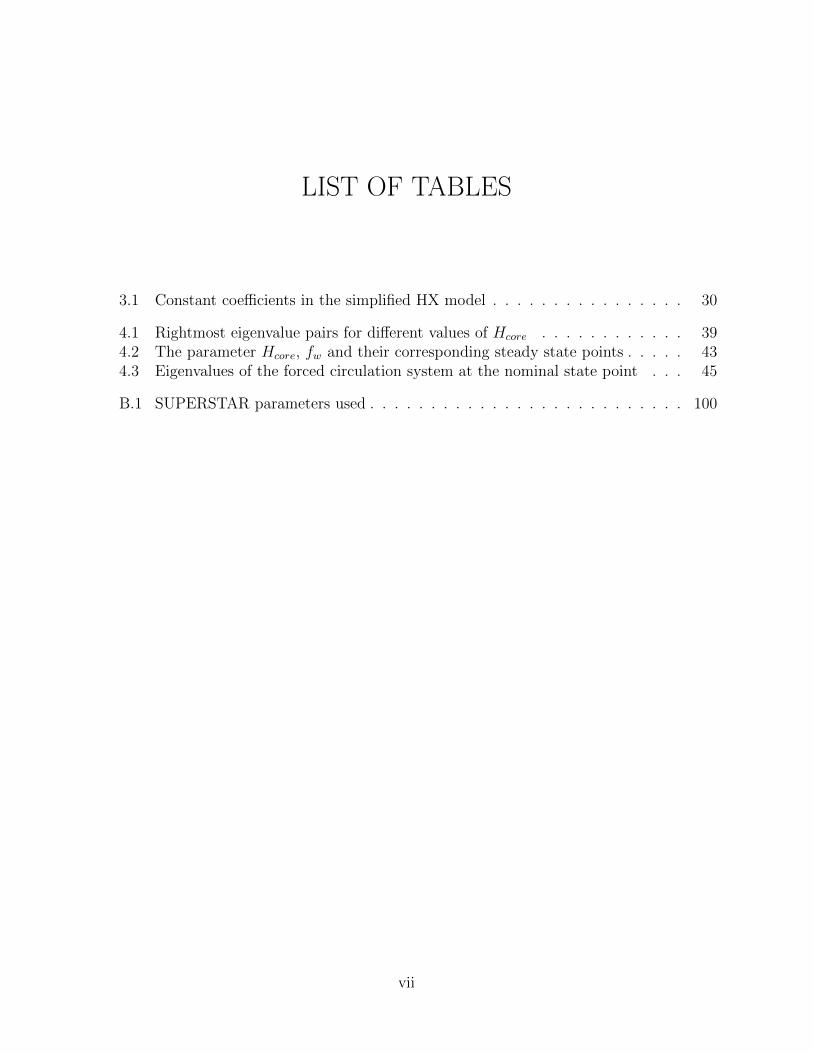
LIST OF TABLES

3.1 Constant coefficients in the simplified HX model . . . . . . . . . . . . . . . . 30

4.1 Rightmost eigenvalue pairs for different values of Hcore . . . . . . . . . . . . 394.2 The parameter Hcore, fw and their corresponding steady state points . . . . . 434.3 Eigenvalues of the forced circulation system at the nominal state point . . . 45

B.1 SUPERSTAR parameters used . . . . . . . . . . . . . . . . . . . . . . . . . . 100

vii

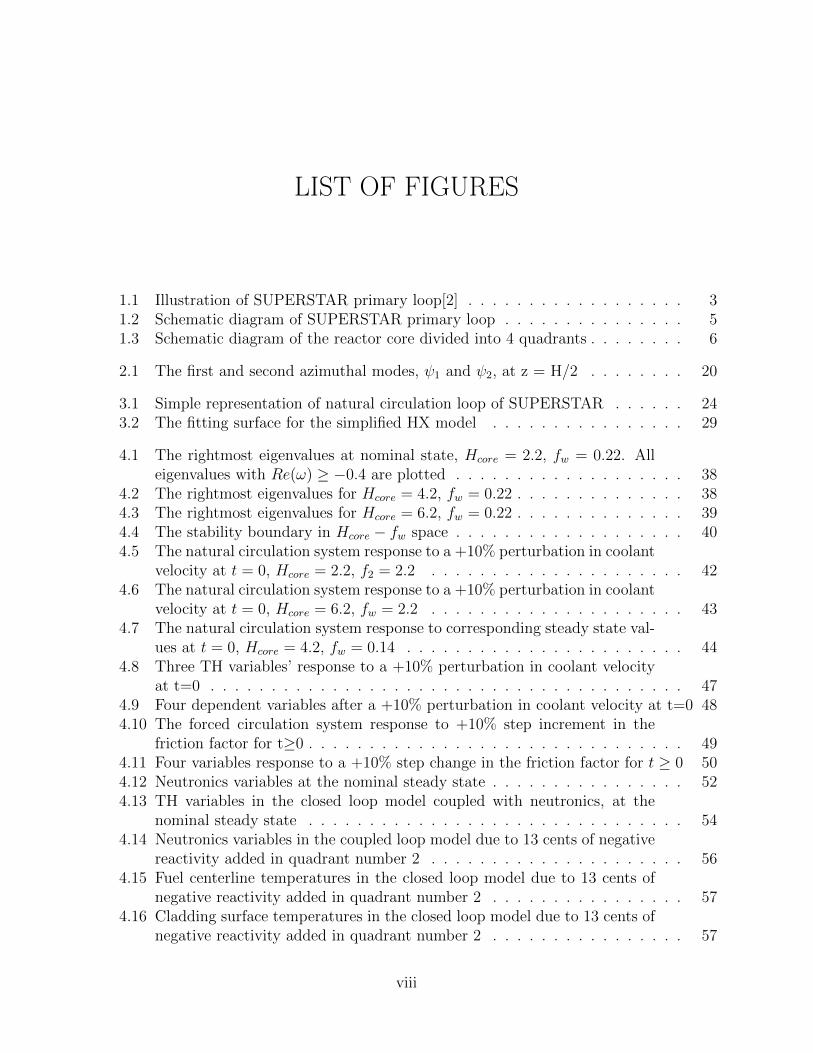
LIST OF FIGURES

1.1 Illustration of SUPERSTAR primary loop[2] . . . . . . . . . . . . . . . . . . 31.2 Schematic diagram of SUPERSTAR primary loop . . . . . . . . . . . . . . . 51.3 Schematic diagram of the reactor core divided into 4 quadrants . . . . . . . . 6

2.1 The first and second azimuthal modes, ψ1 and ψ2, at z = H/2 . . . . . . . . 20

3.1 Simple representation of natural circulation loop of SUPERSTAR . . . . . . 243.2 The fitting surface for the simplified HX model . . . . . . . . . . . . . . . . 29

4.1 The rightmost eigenvalues at nominal state, Hcore = 2.2, fw = 0.22. Alleigenvalues with Re(ω) ≥ −0.4 are plotted . . . . . . . . . . . . . . . . . . . 38

4.2 The rightmost eigenvalues for Hcore = 4.2, fw = 0.22 . . . . . . . . . . . . . . 384.3 The rightmost eigenvalues for Hcore = 6.2, fw = 0.22 . . . . . . . . . . . . . . 394.4 The stability boundary in Hcore − fw space . . . . . . . . . . . . . . . . . . . 404.5 The natural circulation system response to a +10% perturbation in coolant

velocity at t = 0, Hcore = 2.2, f2 = 2.2 . . . . . . . . . . . . . . . . . . . . . 424.6 The natural circulation system response to a +10% perturbation in coolant

velocity at t = 0, Hcore = 6.2, fw = 2.2 . . . . . . . . . . . . . . . . . . . . . 434.7 The natural circulation system response to corresponding steady state val-

ues at t = 0, Hcore = 4.2, fw = 0.14 . . . . . . . . . . . . . . . . . . . . . . . 444.8 Three TH variables’ response to a +10% perturbation in coolant velocity

at t=0 . . . . . . . . . . . . . . . . . . . . . . . . . . . . . . . . . . . . . . . 474.9 Four dependent variables after a +10% perturbation in coolant velocity at t=0 484.10 The forced circulation system response to +10% step increment in the

friction factor for t≥0 . . . . . . . . . . . . . . . . . . . . . . . . . . . . . . . 494.11 Four variables response to a +10% step change in the friction factor for t ≥ 0 504.12 Neutronics variables at the nominal steady state . . . . . . . . . . . . . . . . 524.13 TH variables in the closed loop model coupled with neutronics, at the

nominal steady state . . . . . . . . . . . . . . . . . . . . . . . . . . . . . . . 544.14 Neutronics variables in the coupled loop model due to 13 cents of negative

reactivity added in quadrant number 2 . . . . . . . . . . . . . . . . . . . . . 564.15 Fuel centerline temperatures in the closed loop model due to 13 cents of

negative reactivity added in quadrant number 2 . . . . . . . . . . . . . . . . 574.16 Cladding surface temperatures in the closed loop model due to 13 cents of

negative reactivity added in quadrant number 2 . . . . . . . . . . . . . . . . 57

viii

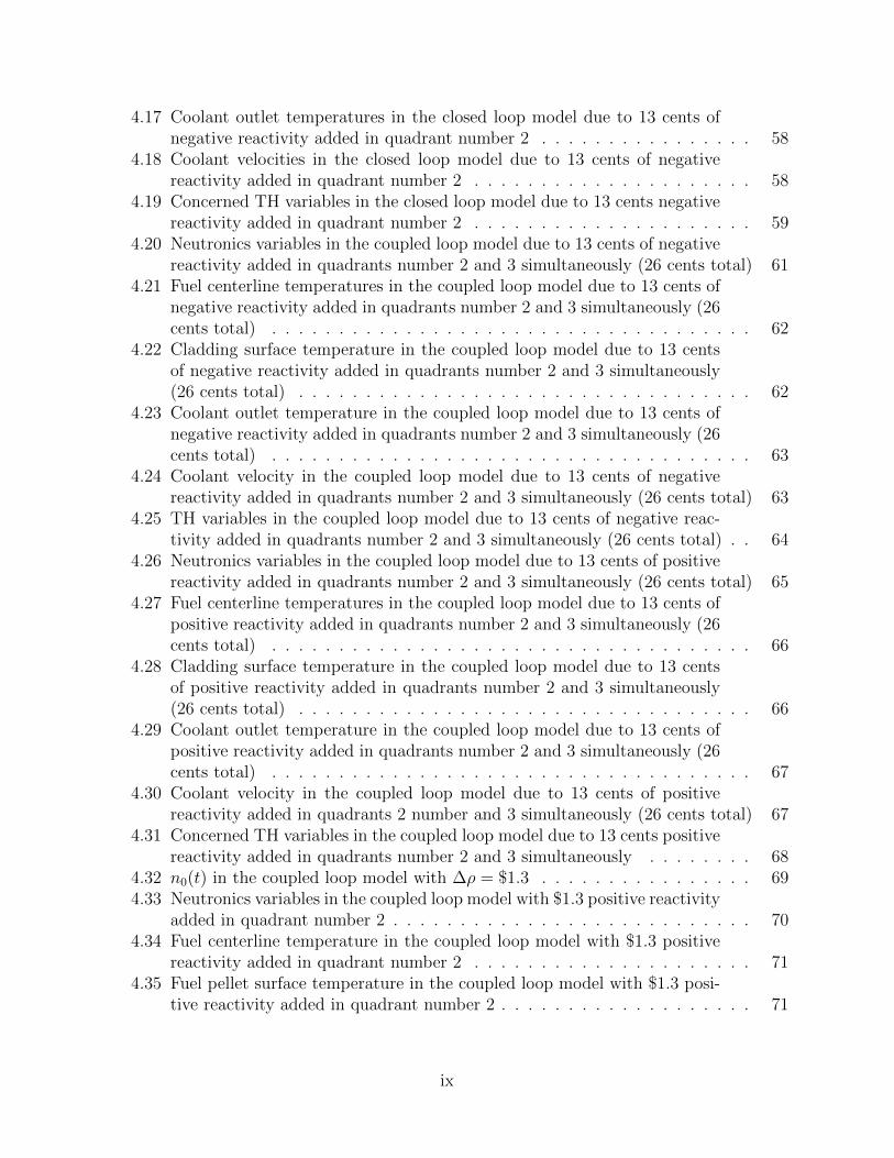
4.17 Coolant outlet temperatures in the closed loop model due to 13 cents ofnegative reactivity added in quadrant number 2 . . . . . . . . . . . . . . . . 58

4.18 Coolant velocities in the closed loop model due to 13 cents of negativereactivity added in quadrant number 2 . . . . . . . . . . . . . . . . . . . . . 58

4.19 Concerned TH variables in the closed loop model due to 13 cents negativereactivity added in quadrant number 2 . . . . . . . . . . . . . . . . . . . . . 59

4.20 Neutronics variables in the coupled loop model due to 13 cents of negativereactivity added in quadrants number 2 and 3 simultaneously (26 cents total) 61

4.21 Fuel centerline temperatures in the coupled loop model due to 13 cents ofnegative reactivity added in quadrants number 2 and 3 simultaneously (26cents total) . . . . . . . . . . . . . . . . . . . . . . . . . . . . . . . . . . . . 62

4.22 Cladding surface temperature in the coupled loop model due to 13 centsof negative reactivity added in quadrants number 2 and 3 simultaneously(26 cents total) . . . . . . . . . . . . . . . . . . . . . . . . . . . . . . . . . . 62

4.23 Coolant outlet temperature in the coupled loop model due to 13 cents ofnegative reactivity added in quadrants number 2 and 3 simultaneously (26cents total) . . . . . . . . . . . . . . . . . . . . . . . . . . . . . . . . . . . . 63

4.24 Coolant velocity in the coupled loop model due to 13 cents of negativereactivity added in quadrants number 2 and 3 simultaneously (26 cents total) 63

4.25 TH variables in the coupled loop model due to 13 cents of negative reac-tivity added in quadrants number 2 and 3 simultaneously (26 cents total) . . 64

4.26 Neutronics variables in the coupled loop model due to 13 cents of positivereactivity added in quadrants number 2 and 3 simultaneously (26 cents total) 65

4.27 Fuel centerline temperatures in the coupled loop model due to 13 cents ofpositive reactivity added in quadrants number 2 and 3 simultaneously (26cents total) . . . . . . . . . . . . . . . . . . . . . . . . . . . . . . . . . . . . 66

4.28 Cladding surface temperature in the coupled loop model due to 13 centsof positive reactivity added in quadrants number 2 and 3 simultaneously(26 cents total) . . . . . . . . . . . . . . . . . . . . . . . . . . . . . . . . . . 66

4.29 Coolant outlet temperature in the coupled loop model due to 13 cents ofpositive reactivity added in quadrants number 2 and 3 simultaneously (26cents total) . . . . . . . . . . . . . . . . . . . . . . . . . . . . . . . . . . . . 67

4.30 Coolant velocity in the coupled loop model due to 13 cents of positivereactivity added in quadrants 2 number and 3 simultaneously (26 cents total) 67

4.31 Concerned TH variables in the coupled loop model due to 13 cents positivereactivity added in quadrants number 2 and 3 simultaneously . . . . . . . . 68

4.32 n0(t) in the coupled loop model with ∆ρ = $1.3 . . . . . . . . . . . . . . . . 694.33 Neutronics variables in the coupled loop model with $1.3 positive reactivity

added in quadrant number 2 . . . . . . . . . . . . . . . . . . . . . . . . . . . 704.34 Fuel centerline temperature in the coupled loop model with $1.3 positive

reactivity added in quadrant number 2 . . . . . . . . . . . . . . . . . . . . . 714.35 Fuel pellet surface temperature in the coupled loop model with $1.3 posi-

tive reactivity added in quadrant number 2 . . . . . . . . . . . . . . . . . . . 71

ix

4.36 Coolant outlet temperature in the coupled loop model with $1.3 positivereactivity added in quadrant number 2 . . . . . . . . . . . . . . . . . . . . . 72

4.37 Neutronics variables in the coupled loop model with $1.3 positive reactivityadded in quadrant number 2 . . . . . . . . . . . . . . . . . . . . . . . . . . . 73

4.38 Fuel centerline temperature in the coupled loop model with $1.3 positivereactivity added in quadrant number 2 . . . . . . . . . . . . . . . . . . . . . 74

4.39 Fuel pellet surface temperature in the coupled loop model with $1.3 posi-tive reactivity added in quadrant number 2 . . . . . . . . . . . . . . . . . . . 74

4.40 Coolant outlet temperature in the coupled loop model with $1.3 positivereactivity added in quadrant number 2 . . . . . . . . . . . . . . . . . . . . . 75

4.41 Neutronics variables in the coupled loop model with a partial blockage inquadrants number 2 and 3 . . . . . . . . . . . . . . . . . . . . . . . . . . . . 76

4.42 Fuel centerline temperatures in the coupled loop model with a blockage inquadrants number 2 and 3 . . . . . . . . . . . . . . . . . . . . . . . . . . . . 77

4.43 Cladding surface temperature in the coupled loop model with a blockagein quadrants number 2 and 3 . . . . . . . . . . . . . . . . . . . . . . . . . . . 77

4.44 Coolant outlet temperature in the coupled loop model with a blockage inquadrants number 2 and 3 . . . . . . . . . . . . . . . . . . . . . . . . . . . . 78

4.45 Coolant velocity in the coupled loop model with a blockage in quadrantsnumber 2 and 3 . . . . . . . . . . . . . . . . . . . . . . . . . . . . . . . . . . 78

4.46 TH variables for quadrant number 2 in the coupled loop model with ablockage in quadrants number 2 and 3 . . . . . . . . . . . . . . . . . . . . . 79

4.47 TH variables for quadrant number 1 in the coupled loop model with ablockage in quadrants number 2 and 3 . . . . . . . . . . . . . . . . . . . . . 79

4.48 TH variables in the coupled loop model with a +10% change in Tci inquadrant number 1 over 5 5 t 5 15 s . . . . . . . . . . . . . . . . . . . . . . 81

4.49 Fuel centerline and cladding surface temperature in the coupled loop modelwith a +10% change in Tci in quadrant number 1 over 5 5 t 5 15 s . . . . . 81

4.50 Neutronics variables in the coupled loop model with a +10% change in Tciin quadrant number 1 over 5 5 t 5 15 s . . . . . . . . . . . . . . . . . . . . . 82

4.51 n0(t) comparison in the coupled loop between point kinetics and multi-modes model, with the same perturbation as in scenario 2 . . . . . . . . . . 83

4.52 T0(t) comparison in the coupled loop between point kinetics and multi-modes model, with the same perturbation as in scenario 2 . . . . . . . . . . 84

4.53 Comparison of cladding surface temperatures in the coupled loop betweenpoint kinetics and multi-modes model, with the same perturbation as inscenario 2 . . . . . . . . . . . . . . . . . . . . . . . . . . . . . . . . . . . . . 85

4.54 Comparison of coolant outlet temperature in the coupled loop betweenpoint kinetics and multi-modes model, with the same perturbation as inscenario 2 . . . . . . . . . . . . . . . . . . . . . . . . . . . . . . . . . . . . . 85

4.55 Comparison of coolant velocity in the coupled loop between point kineticsand multi-modes model, with the same perturbation as in scenario 2 . . . . . 86

4.56 Neutronics variables with longer than nominal time delays, τ1 = 70, τ2 = 43 . 874.57 Neutronics variables with shorter than nominal time delays, τ1 = 55, τ2 = 28 88

x

4.58 TH variables with longer than nominal time delays, τ1 = 70, τ2 = 43 . . . . . 894.59 TH variables with shorter than nominal time delays, τ1 = 55, τ2 = 28 . . . . 894.60 TH variables with longer than nominal time delays, τ1 = 80, τ2 = 53 . . . . . 90

5.1 Coefficient of the linear term in the coolant axial temp profile, a1(t) . . . . . 925.2 Coefficient of the quadratic term in the coolant axial temp profile, a2(t) . . . 92

C.1 Schematic illustration of fuel rod [9] . . . . . . . . . . . . . . . . . . . . . . . 102

D.1 Simple representation of natural circulation loop of SUPERSTAR . . . . . . 112

F.1 Schematic illustration of SUPERSTAR fuel assembly geometry in SERPENT 121F.2 Macroscopic fission and absorption cross section variation with normalized

fuel temperature . . . . . . . . . . . . . . . . . . . . . . . . . . . . . . . . . 122

xi

LIST OF ABBREVIATIONS

ANL Argonne National Laboratory

CR Conversion Ratio

DDE Delay Differential Equation

ELSY European Lead-cooled SYstem

FPHE Formed Plate Heat Exchanger

HX Heat eXchanger

IHX Intermediate Heat eXchanger

LBE Lead-Bismuth Eutectic

LFR Lead-cooled Fast Reactors

LHMC Liquid Heavy Metal Cooled

NPP Nuclear Power Plant

PCHE Printed Circuit Heat Exchanger

SG Steam Generator

SMR Small Modular Reactor

SSTAR Small Secure Transportable Autonomous Reactor

STAR Secure Transportable Autonomous Reactor

STAR-LM Secure Transportable Autonomous Reactor with Liquid Metal

SUPERSTAR SUstainable Proliferation-resistance Enhanced Refined Secure TransportableAutonomous Reactor

xii

CHAPTER 1

INTRODUCTION

In a surge of interest in nuclear energy in recent years, a significant amount of effort

has been devoted to developing innovative reactor types, and to make current ones more

economically efficient. These efforts include the reactor titled SUPERSTAR which is the

focus of this work. This dissertation is aimed at assessing the stability of SUPERSTAR.

This chapter is composed of three sections: section 1.1 is a brief overview of SUPERSTAR.

Previous work and literature review can be found in section 1.2. Section 1.3 discusses the

technical scope of this work.

1.1 SUPERSTAR system

This section includes two parts: First, the background and motivation of SUPERSTAR

are described. Second, the geometry of SUPERSTAR based on its preliminary design is

illustrated.

1.1.1 Background and motivation

Fast reactors have several advantages over thermal reactors. Unlike more popular Sodium-

cooled fast reactors, the Liquid Heavy Metal Cooled (LHMC) reactors use metal with high

density, such as lead or lead-bismuth eutectic as coolant. The only Lead-cooled Fast Reactors

(LFR) that have been constructed and operated are the Lead-Bismuth Eutectic (LBE) cooled

submarine reactors and land prototypes in the Soviet Union and subsequently the Russian

Federation[1]. So far, a LFR has never been operated commercially.

1

Argonne National Laboratory (ANL) has studied the Secure Transportable Autonomous

Reactor with Liquid Metal (STAR-LM) and Small Secure Transportable Autonomous Re-

actor (SSTAR) concepts since 1997 as well as the European Lead-cooled SYstem (ELSY)

since about 2005[1]. The work on a first-of-a-kind demonstration of a pre-conceptual de-

sign for an improved Secure Transportable Autonomous Reactor (STAR) has been carried

out at ANL, and is named the SUstainable Proliferation-resistance Enhanced Refined Secure

Transportable Autonomous Reactor (SUPERSTAR). It incorporates lessons learned, inno-

vations, and best features from previous STAR and ELSY developments as well as other

developments[1].

SUPERSTAR, being developed at ANL, is an improved ∼120 MWe (300 MWt) Pb-cooled,

pool-type, small modular fast reactor for international or remote deployment. Initial efforts

have focused on a near-term deployable SUPERSTAR demonstrator (demo) representing a

first-of-a-kind deployment. SUPERSTAR development seeks to achieve the largest thermal

power limited by primary Pb coolant natural circulation heat transport inside of a reactor

vessel, and guard vessel having dimensions limited by the requirement of transportability

by rail. The objective is to maximize the economic performance of a transportable natural

circulation LFR as measured by the capital cost per unit electrical power[2].

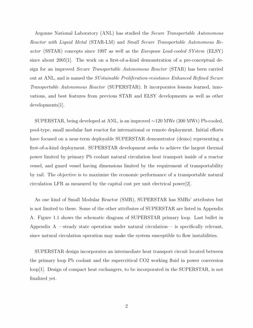
As one kind of Small Modular Reactor (SMR), SUPERSTAR has SMRs’ attributes but

is not limited to these. Some of the other attributes of SUPERSTAR are listed in Appendix

A. Figure 1.1 shows the schematic diagram of SUPERSTAR primary loop. Last bullet in

Appendix A —steady state operation under natural circulation— is specifically relevant,

since natural circulation operation may make the system susceptible to flow instabilities.

SUPERSTAR design incorporates an intermediate heat transport circuit located between

the primary loop Pb coolant and the supercritical CO2 working fluid in power conversion

loop[1]. Design of compact heat exchangers, to be incorporated in the SUPERSTAR, is not

finalized yet.

2

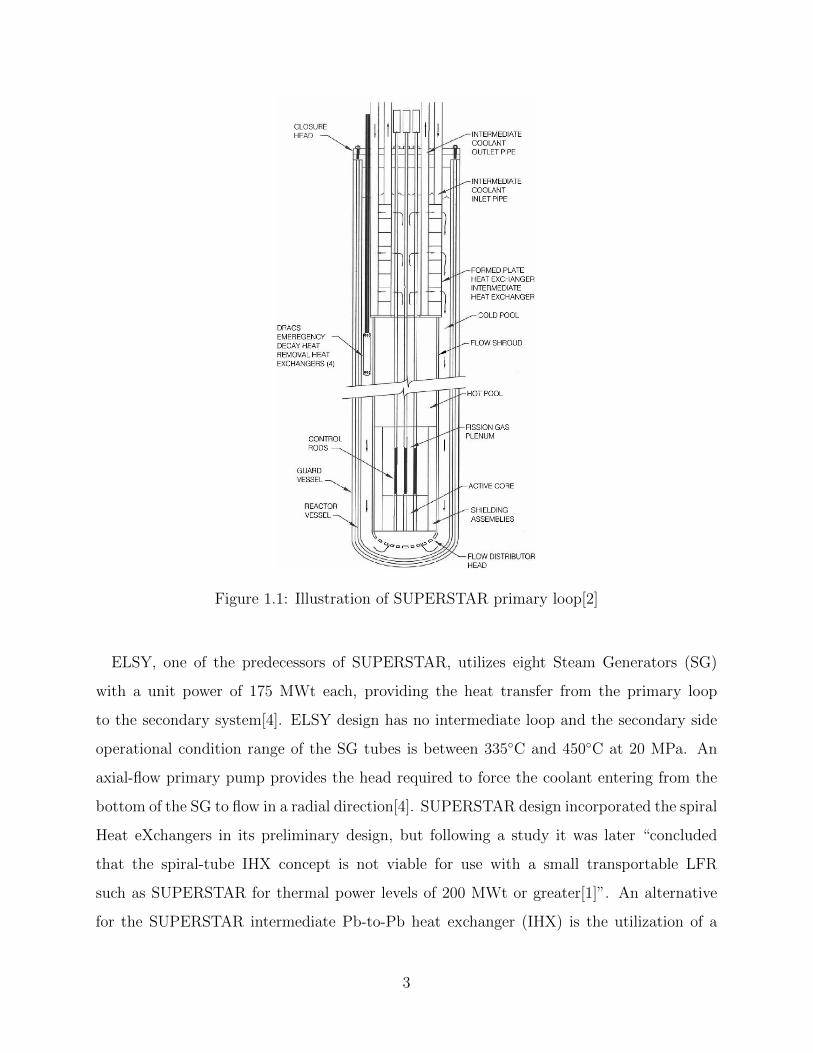
Figure 1.1: Illustration of SUPERSTAR primary loop[2]

ELSY, one of the predecessors of SUPERSTAR, utilizes eight Steam Generators (SG)

with a unit power of 175 MWt each, providing the heat transfer from the primary loop

to the secondary system[4]. ELSY design has no intermediate loop and the secondary side

operational condition range of the SG tubes is between 335◦C and 450◦C at 20 MPa. An

axial-flow primary pump provides the head required to force the coolant entering from the

bottom of the SG to flow in a radial direction[4]. SUPERSTAR design incorporated the spiral

Heat eXchangers in its preliminary design, but following a study it was later “concluded

that the spiral-tube IHX concept is not viable for use with a small transportable LFR

such as SUPERSTAR for thermal power levels of 200 MWt or greater[1]”. An alternative

for the SUPERSTAR intermediate Pb-to-Pb heat exchanger (IHX) is the utilization of a

3

compact diffusion-bonded heat exchanger such as a Printed Circuit Heat Exchanger (PCHE)

or Formed Plate Heat Exchanger (FPHE) developed by Heatric Inc.[1].

Preliminary work on SUPERSTAR carried out thus far has included the development of a

completely new pre-conceptual design of the core, primary coolant system, and intermediate

coolant system[1].

Unlike forced circulation reactors that rely on recirculation pumps in the primary loop,

SUPERSTAR relies on natural circulation in the primary loop, which is maintained by the

coolant density difference caused by the temperature variation. The pressure drop along

the flow path is compensated by the head due to the density difference. Loops that rely on

natural circulation, and hence SUPERSTAR, though desirable under accidental scenarios

to extract decay heat, are more susceptible to flow instabilities. Furthermore, when the

neutronics model is coupled with the thermal-hydraulics model, various feedback mecha-

nisms add to the complexity. Hence, it is important to study the stability characteristics of

SUPERSTAR.

1.1.2 Reactor geometry

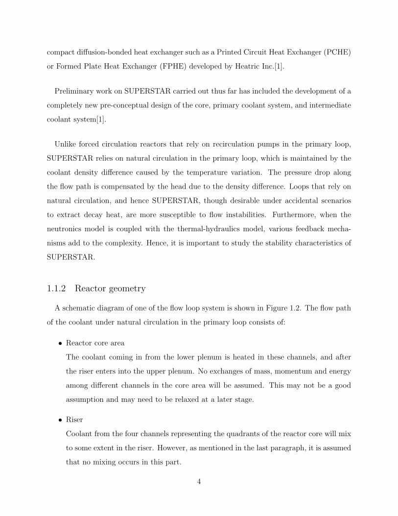
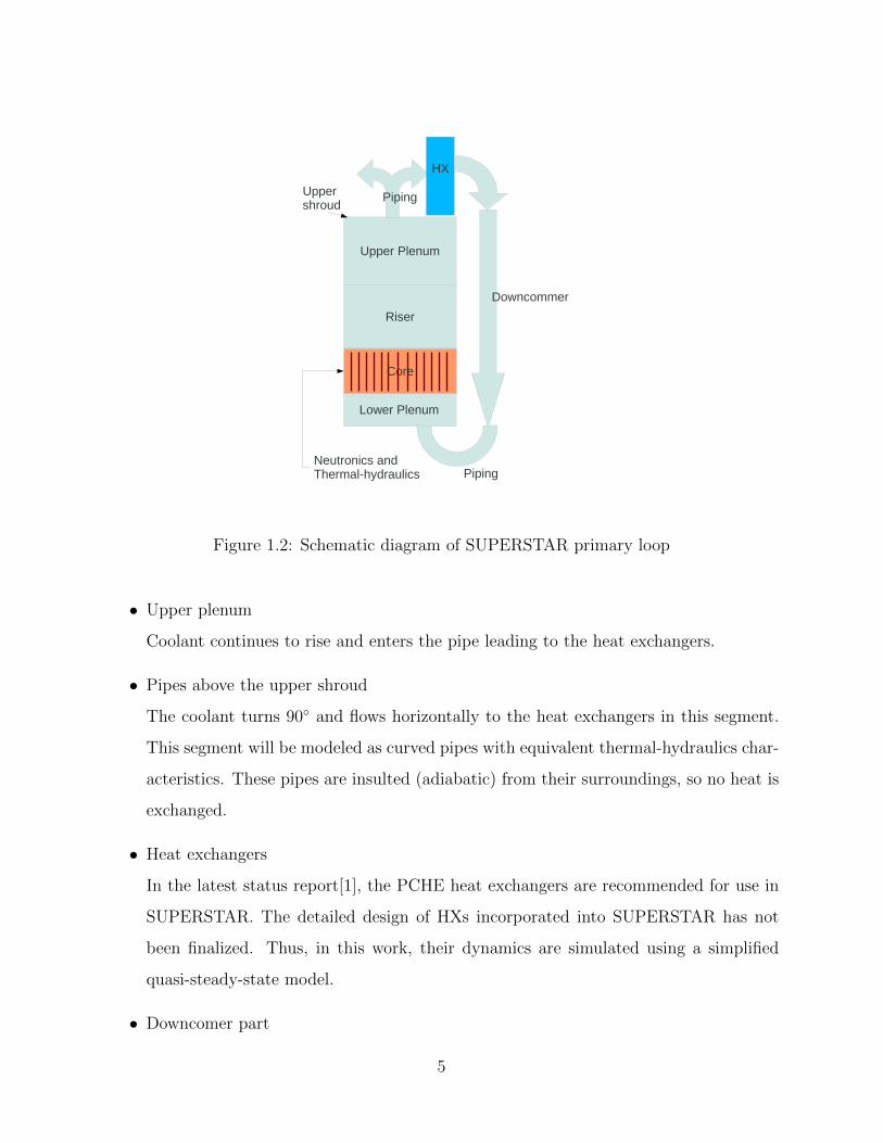
A schematic diagram of one of the flow loop system is shown in Figure 1.2. The flow path

of the coolant under natural circulation in the primary loop consists of:

• Reactor core area

The coolant coming in from the lower plenum is heated in these channels, and after

the riser enters into the upper plenum. No exchanges of mass, momentum and energy

among different channels in the core area will be assumed. This may not be a good

assumption and may need to be relaxed at a later stage.

• Riser

Coolant from the four channels representing the quadrants of the reactor core will mix

to some extent in the riser. However, as mentioned in the last paragraph, it is assumed

that no mixing occurs in this part.

4

Core

Upper Plenum

Piping

HX

Downcommer

Piping

Lower Plenum

Riser

Uppershroud

Neutronics and Thermal-hydraulics

Figure 1.2: Schematic diagram of SUPERSTAR primary loop

• Upper plenum

Coolant continues to rise and enters the pipe leading to the heat exchangers.

• Pipes above the upper shroud

The coolant turns 90◦ and flows horizontally to the heat exchangers in this segment.

This segment will be modeled as curved pipes with equivalent thermal-hydraulics char-

acteristics. These pipes are insulted (adiabatic) from their surroundings, so no heat is

exchanged.

• Heat exchangers

In the latest status report[1], the PCHE heat exchangers are recommended for use in

SUPERSTAR. The detailed design of HXs incorporated into SUPERSTAR has not

been finalized. Thus, in this work, their dynamics are simulated using a simplified

quasi-steady-state model.

• Downcomer part

5

The coolant changes its direction twice in this segment. After exiting from the heat

exchangers horizontally, the coolant turns 90◦ and flows downward. At the bottom of

the downcommer, the coolant turns 180◦ to enter the lower plenum.

• Lower plenum

Coolant from the four loops enters the distributor in this region and flows to the

corresponding heated channels.

In this work, the segments along the flow path are modeled as equivalent pipes, and adiabatic

wall boundary condition is applied. Therefore, heat transfer takes place only in the heated

channels and the HXs.

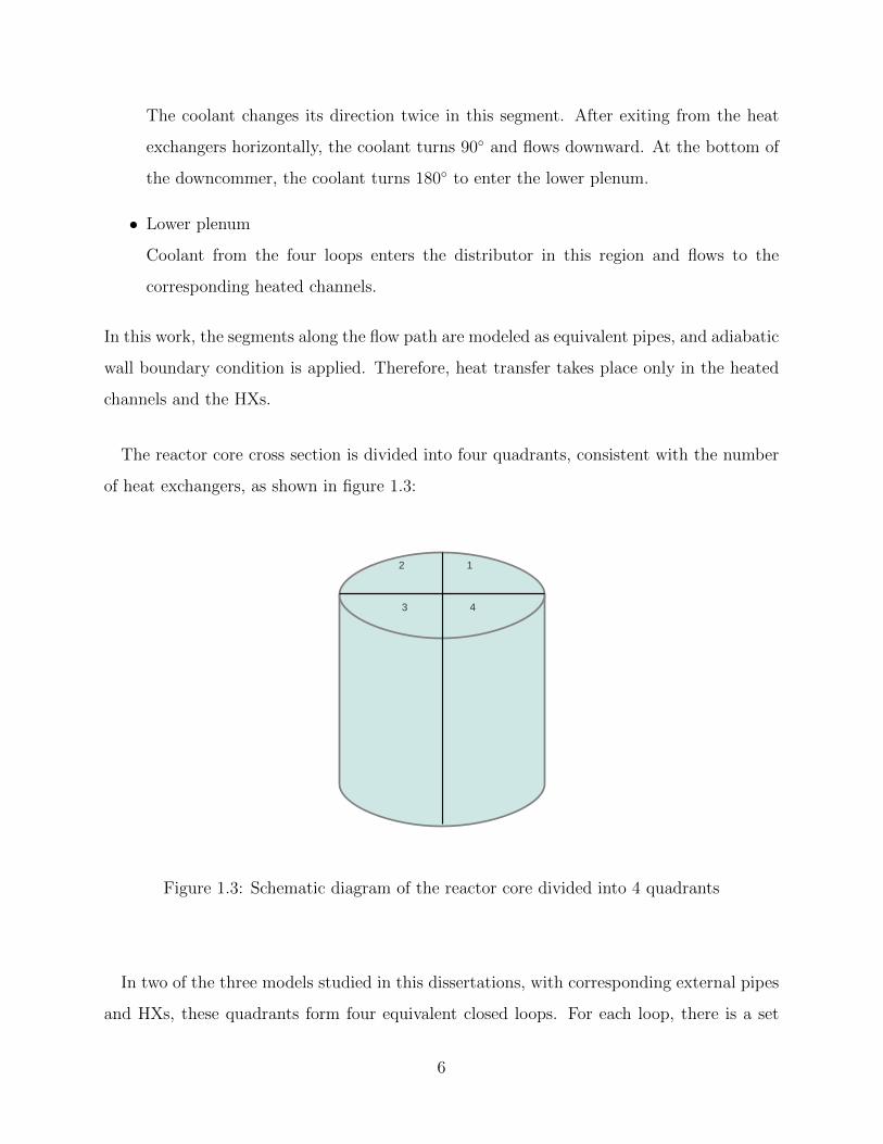
The reactor core cross section is divided into four quadrants, consistent with the number

of heat exchangers, as shown in figure 1.3:

2 1

3 4

Figure 1.3: Schematic diagram of the reactor core divided into 4 quadrants

In two of the three models studied in this dissertations, with corresponding external pipes

and HXs, these quadrants form four equivalent closed loops. For each loop, there is a set

6

of TH variables identified by different subscripts. By setting different parameter values for

each loop, asymmetry is introduced among the loops and corresponding regional effects can

be studied.

1.2 Previous work and literature review

Status of research on SUPERSTAR can be found in references [1], [2] and [3]. Parameter

values and specifications of the reactor core needed in this work are also drawn from these

references. The similar and predecessor system, ELSY, is described in [4] and the pre-

conceptual core design for a high-flux LFR system is discussed in [5]. Overview of current

research on lead-cooled fast reactors is summarized in [6]. Fast breeder reactors are discussed

systematically in reference [7], which also provides reference values for some parameters used

in this work. With modal expansion methods, stability analyses have been done for BWR

system in [8][9][10][11][12][13]. Stability concerns in BWR system which are characterized

with two-phase flow phenomena are discussed in [14]. Stability concerns also exist in other

single-phase flow system and some of these are analyzed in [15][16][17][18]. The modal

expansion methods for nuetronics are further discussed in literature [19][20][21][22].

To model the feedback effects, the cross section dependence on the fuel temperature is

calculated using the SERPENT code, which is fully described in [23]. To verify the capture

of regional effects with higher modes, the higher-mode model for neutronics is compared

with the point kinetics model which follows the convention in [24]. The comparison of

MOX and metallic fuel under externally-induced reactivity perturbations are explored in

[25]. Some data of the metallic fuel such as thermal conductivity and specific heat are listed

in [26]. An innovative particulate metallic fuel design from ANL is presented in [27]. The

characteristics and design considerations for compact heat exchangers which are incorporated

in SUPERSTAR, are discussed in [28], and based on that, a simplified HX model is used in

this work.

7

Properties and the equations of state for lead can be found in [29]. The thermal-hydraulics

concepts and equations follow the convention in [30][31] and [32]. The reference [33] covers

the conventional heat transfer phenomena. The latter two references also provide the fuel

pin heat conduction model. The derivation of governing equations for the coolant also refers

to [9][10][34] and [35]. Especially, the time-dependent momentum equations for the natural

circulation loop is developed from the steady state momentum equation which is discussed in

[34]. Detailed sub-channel analysis for LBE-cooled faster reactor is carried out in reference

[36]. The axial conduction effect on the liquid metal system is discussed in [37] which also

acts as a verification for some of the results in this work.

In order to reduce the time- and space-dependent PDEs to ODEs, the weighted residual

method is used in this work. This method can be found in reference [38]. Due to the time

delays present in the flow loop model, systems finally are described by sets of delay differential

equations (DDEs), given that HXs are incorporated into the loop. The characteristics and

stability analyses are explored in [39][40] and [41]. In this work, a MATLAB package named

DDE-BIFTOOL, is used to carry out the stability analysis in frequency domain which is

fully described in [42].

1.3 Scope of this dissertation

Since SUPERSTAR is first-of-a-kind demonstrator reactor, little work has been done on

its stability compared to the extensive body of work on boiling water reactors[8][9][10][11].

This dissertation focuses on the stability analysis of SUPERSTAR, modeled using its neu-

tronics coupled with thermal-hydraulics. It is based on a reduced order model, and provides

guidances and recommendations on its design.

For neutronics, although point kinetics equations are often used for fast reactors[7], due to

spatial feedback effects and due to the possibility of out-of-phase instabilities in the reactor

core, modal analysis needs to be employed including the higher order modes. Stacey[19] lists

several options for modal expansion, including λ−modes, ω−modes, synthesis modes, etc.

8

In this work, the synthesis modes method[19][20] will be utilized. Akcasu et al.[21] outline

the method to find the weighted function matrix used in this method. Mathematically, a

constraint on choosing mode functions is that they should be orthogonal over the domain[22].

For thermal-hydraulics, though routinely used for steady-state and core-only analyses,

solving the time-dependent three-dimensional mass, momentum and energy equations, for

the primary loop even when the coolant is in single-phase, is currently not possible. Thus,

reduced order models are often needed to carry out stability analysis. Reduced order mod-

els for BWRs have been developed and studied[8][9][10][11]. In this study, each quadrant

in the reduced order model will be represented by a one-dimensional channel. Thermal-

hydraulics parameters for this channel will be equivalent to the lumped parameters obtained

by averaging over all flow channels in this quadrant.

While the primary driver for instability is the natural circulation thermal-hydraulics,

neutronics, due to temperature feedback, can also play a role, and hence nuclear-coupled

thermal-hydraulics of the core and thermal-hydraulics of the rest of the flow loop must be

included in any stability analysis. The feedback effects due to different mechanisms are

assumed to be spontaneous and they are integrated into a linear feedback model. This

model links fuel temperatures and macroscopic cross sections. This model is developed

using SERPENT[23].

Thus, a reduced order model that includes coupled neutronics and thermal-hydraulics for

the core and natural circulation thermal-hydraulics for the rest of the loop is developed, and

then used to carry out stability analysis.

Rather than numerically solving the PDEs directly[18], weighted residual method is used

to convert the PDEs to ODEs[9][10]. For the heat conduction model for fuel pins, variational

method is often used to convert the PDEs to ODEs[9][10]. However, the metallic fuel in-

corporated in SUPERSTAR flattens its temperature distribution profile. Hence, a weighted

residual method is sufficient to capture this distribution and reduce these PDEs to ODEs.

The thermal-hydraulics system thus can be described by a set of ODEs. In this work, all

9

PDEs are converted to ODEs using the weighted residual method. Depending on whether

time delays are included or not in the loop, these ODEs might be classified as DDEs (ODEs

with time delays). Stability analyses for this system are then carried out using the set of

ODEs/DDEs.

This dissertation is arranged as follows: The modal expansion method for neutronics is

described in Chapter 2; Chapter 3 discusses the primary coolant system, the reduced order

model and heat conduction model for thermal-hydraulics, also presents the simplified model

of HXs; stability analyses under different scenarios, based on three models developed, are

carried out in Chapter 4; and Chapter 5 discusses the verification and validation of the

model; Chapter 6 presents the conclusion and suggested future work.

10

CHAPTER 2

NEUTRONICS MODEL USING MODAL ANALYSIS

Stability analyses of Nuclear Power Plants (NPPs) are often carried out using the point

reactor kinetics equation. However, point kinetics is based on the assumption that the

spatial component of the flux profile (reactor power distribution) remains fixed, while the

total neutron population and hence, power changes with time. This limitation, for a single

spatial mode case, renders the reactor as a ‘point’, which cannot capture or simulate regional

effects, that may result from, for example, local variations in core thermal hydraulics. Modal

expansion method can be extended to include spatial effects along the azimuthal direction

by including the fundamental as well as higher order modes in that direction.

The one-group neutron diffusion equations with one group effective delayed neutron pre-

cursor (using conventional symbols)[24] are:

v∗−1∂φ∗(rrr∗, t∗)

∂t∗= [∇ ·D∇− Σa + (1− βe)νΣf ]φ

∗(rrr∗, t∗) + λC∗(rrr∗, t∗) (2.1)

∂C∗(rrr∗, t∗)

∂t∗= βeνΣfφ

∗(rrr∗, t∗)− λC∗(rrr∗, t∗) (2.2)

Here and after, ‘∗’ means that physical values are dimensional (this convention is not ap-

plied on nuclear property symbols such as D,Σf ,Σa, λ). The flux in the modal expansion

method[19][22] is written as:

φ∗(rrr∗, t∗) = v∗ ·J−1∑j=0

ψ∗j (rrr∗)n∗j(t

∗) (2.3)

11

which, in matrix form, can also be rewritten as

φ∗(rrr∗, t∗) = v∗ ·ψ∗ψ∗ψ∗(rrr∗)nnn∗(t∗) (2.4)

where

ψ∗ψ∗ψ∗(rrr∗) =[ψ∗0(rrr∗) ψ∗1(rrr∗) · · · ψ∗J−1(rrr∗)

]and

n∗n∗n∗(t∗) =

n∗0(t∗)

n∗1(t∗)...

n∗J−1(t∗)

Assuming the precursor concentration to have the same spatial profile as the neutron flux[19][22],

C∗(rrr∗, t∗) = ψ∗ψ∗ψ∗(rrr∗)ξξξ∗(t∗) (2.5)

where

ξ∗ξ∗ξ∗(t∗) =

ξ∗0(t∗)

ξ∗1(t∗)...

ξ∗J−1(t∗)

ψψψ∗, the shape factor, is a 1× J matrix with elements ψ∗j , J is the number of modes kept,

while nnn∗, the amplitude factor, is a J × 1 matrix with elements n∗j . Here j = 0, ...J − 1. The

physical meanings of n∗j(t∗) can be explained this way: if we normalize the shape factor over

the volume domain,∫d3r∗ψ∗j = 1, the coefficients n∗j(t

∗) then represent the total number of

neutrons in the jth mode in the reactor at time t∗[19][22]. ξξξ∗(t∗) is the amplitude factor of

precursor concentration with elements ξ∗j (t∗). ψ∗j (rrr

∗) are the eigenfunctions of the critical

reactor. Substituting equations (2.4) and (2.5) into equation (2.1), and realizing that only

12

a finite number of modes J are being kept in the analysis, the residual R is given by

R = ψψψ∗dnnn∗

dt∗− v∗ · [∇ ·D∇− Σa + (1− βe)νΣf ]ψψψ

∗nnn∗ − λψψψ∗ξξξ∗ (2.6)

where R is the residual scalar. Introducing the weight function matrix WWW

[W0 W1 · · · WJ−1

]and multiplying both sides of equation (2.6) with its transpose matrix WWW T , and integrating

the left-hand side over the volume of the whole core, we require this integral of the weighted

residual to be zero ∫WWW TRd3r∗ = 0 (2.7)

Carrying out this operation on the RHS of equation (2.6) requires us to realize that there

are four reactivity feedback mechanisms considered in this work. They are lead density,

axial expansion, radial expansion and Doppler effects. The first three effects are assumed

to be occur instantaneously after the change in fuel temperature, and are merged in the

Doppler effect. This (modified) time-dependent Doppler effect is modeled by introducing a

time-dependent relation between the cross section and the fuel temperature σ = σ(T (t)).

Consistent with the thermal hydraulic model, the whole reactor core is divided into four

quadrants. With fuel temperature feedback and other effects, the macroscopic cross sections

in each channel might be different because the thermal hydraulics processes evolve separately

in each quadrant and the cross sections are functions of local fuel temperatures. So, the

integral over the volume with respect to cross sections on the right-hand side of equation

(2.6) should be split into four segments corresponding to the four quadrants[12][13]. For

leakage and delayed neutrons terms, the integral can be taken over the whole core volume

because both the diffusion length D and the decay constant λ are assumed to be constant

13

across the whole core. Thus, we have(∫WWW Tψψψ∗d3rrr

)dnnn∗

dt∗= v∗ ·

(∫WWW TD∇2ψψψ∗d3rrr∗

)nnn∗

+v∗ · (−Σa,Q1 + (1− βe) · νΣf,Q1) ·∫Q1

W Tψψψ∗d3rrr∗ · nnn∗

+v∗ · (−Σa,Q2 + (1− βe) · νΣf,Q2) ·∫Q2


+v∗ · (−Σa,Q3 + (1− βe) · νΣf,Q3) ·∫Q3


+v∗ · (−Σa,Q4 + (1− βe) · νΣf,Q4) ·∫Q4


+λ

(∫WWW Tψψψ∗d3rrr∗

)ξξξ∗

(2.8)

Similarly, for equation (2.2) we have

(∫WWW Tψψψ∗d3r∗

)dξξξ∗

dt∗= v∗ · βeνΣf,Q1 ·

∫Q1

W Tψψψ∗d3r∗ · nnn∗

+v∗ · βeνΣf,Q2 ·∫Q2






−λ(∫

WWW Tψψψ∗d3r∗)ξξξ∗

(2.9)

Here, Q1, Q2, Q3 and Q4 represent quadrant 1 through 4, respectively. Now defining three

3× 3 matrices (ΦΦΦ, ρρρ and βββ) as

ΦΦΦ ≡∫WWW Tψψψ∗d3r∗ (2.10)

14

ρρρ ≡ v∗ ·∫WWW TD∇2ψψψ∗d3rrr∗

+v∗ · (−Σa,Q1 + ·νΣf,Q1) ·∫Q1

W Tψψψ∗d3rrr∗

+v∗ · (−Σa,Q2 + ·νΣf,Q2) ·∫Q2


+v∗ · (−Σa,Q3 + ·νΣf,Q3) ·∫Q3


+v∗ · (−Σa,Q4 + ·νΣf,Q4) ·∫Q4


(2.11)

and

βββ ≡ v∗ · βe · νΣf,Q1 ·∫Q1


+v∗ · βe · νΣf,Q2 ·∫Q2


+v∗ · βe · νΣf,Q3 ·∫Q3


+v∗ · βe · νΣf,Q4 ·∫Q4


(2.12)

equations (2.8) and (2.9) can be written as

ΦΦΦdnnn∗

dt∗= (ρρρ− βββ)nnn∗ + λΦΦΦξξξ∗ (2.13)

ΦΦΦdξξξ∗

dt∗= βββnnn∗ − λΦΦΦξξξ∗ (2.14)

Equations (2.13) and (2.14) are sets of ODEs called “multi-mode kinetics equations”[19].

Note for the conventional reactivity, ρρρ should be scaled by Λ which is the generation time of

neutrons.

15

Multiplying both sides by the inverse of ΦΦΦ, we have

dnnn∗

dt∗= v∗ ·D ·ΦΦΦ−1 ·

∫W T∇2ψψψ∗d3rrr∗ · nnn∗

+v∗ · (−Σa,Q1 + (1− βe) · νΣf,Q1) ·ΦΦΦ−1 ·∫Q1


+v∗ · (−Σa,Q2 + (1− βe) · νΣf,Q2) ·ΦΦΦ−1 ·∫Q2


+v∗ · (−Σa,Q3 + (1− βe) · νΣf,Q3) ·ΦΦΦ−1 ·∫Q3


+v∗ · (−Σa,Q4 + (1− βe) · νΣf,Q4) ·ΦΦΦ−1 ·∫Q4


+λIII · ξξξ∗

(2.15)

dξξξ∗

dt∗= v∗ · βe · νΣf,Q1 ·ΦΦΦ−1 ·

∫Q1


+v∗ · βe · νΣf,Q2 ·ΦΦΦ−1 ·∫Q2


+v∗ · βe · νΣf,Q3 ·ΦΦΦ−1 ·∫Q3


+v∗ · βe · νΣf,Q4 ·ΦΦΦ−1 ·∫Q4


−λIII · ξξξ∗

(2.16)

16

By choosing nnnref the value of n∗n∗n∗(t) at steady state, we have the dimensionless form of the

set of equations

dnnn

dt=L∗refv∗ref

· v∗ ·D ·ΦΦΦ−1 ·∫W T∇2ψψψ∗d3r∗ · nnn

+L∗refv∗ref

· v∗ · (−Σa,Q1 + (1− βe) · νΣf,Q1) ·ΦΦΦ−1 ·∫Q1

W Tψψψ∗d3r∗ · nnn

+L∗refv∗ref

· v∗ · (−Σa,Q2 + (1− βe) · νΣf,Q2) ·ΦΦΦ−1 ·∫Q2


+L∗refv∗ref

· v∗ · (−Σa,Q3 + (1− βe) · νΣf,Q3) ·ΦΦΦ−1 ·∫Q3


+L∗refv∗ref

· v∗ · (−Σa,Q4 + (1− βe) · νΣf,Q4) ·ΦΦΦ−1 ·∫Q4


+L∗refv∗ref

· λIII · ξξξ

(2.17)

dξξξ

dt=L∗refv∗ref

· v∗ · βeνΣf,Q1 ·ΦΦΦ−1 ·∫Q1


+L∗refv∗ref



+L∗refv∗ref



+L∗refv∗ref



−L∗refv∗ref

· λIII · ξξξ

(2.18)

where nnn = nnn∗/nnnref and ξξξ = ξξξ∗/nnnref . This is the set of ODE for neutronics which includes

six equations for n0(t), n1(t), n2(t), ξ0(t), ξ1(t) and ξ2(t), given that the first three modes

ψ∗0(r∗), ψ∗1(r∗) and ψ∗2(r∗) are retained. Although the equations above for nnn and ξξξ are

dimensionless, the integral over the quadrants and the integral over the entire domain in

the leakage term take place in dimensional domain. Some further details related to these

equations are discussed below.

In this work, we assume that absorption cross section and fission cross section vary linearly

with the averaged fuel temperature which is calculated based on the single fuel pin heat

17

conduction model. So, we have

Σa(t) = Σa,ref +∂Σa

∂Tfuel,ave· (Tfuel,ave(t)− Tfuel,ref ) (2.19)

Σf (t) = Σf,ref +∂Σf

∂Tfuel,ave· (Tfuel,ave(t)− Tfuel,ref ) (2.20)

where, Tfuel,ave(t) is the non-dimensional fuel temperature averaged across the radial direc-

tion, therefore, both the absorption and fission macro cross sections are time-dependent.

The slopes describing linear dependencies between cross sections and temperature in

equations (2.19) and (2.20) are calculated using the SERPENT code. “Serpent is a three-

dimensional, continuous-energy Monte Carlo reactor physics burnup calculation code specifi-

cally designed for lattice physics applications”[23]. Homogenized multi-group constants such

as macroscopic cross sections can be generated by Serpent and printed in the standard out-

put. By specifying the nuclides name at different temperatures in the material entry in the

input cards, the macroscopic cross sections at corresponding temperatures can be retrieved

in the output file. Hence, the linear dependency can be generated. The details are included

in appendix E.

The derivation above is for one energy group. In this work, one-group analysis is considered

sufficient. The choice of one-group neutron kinetics is based on the fact that in fast reactors,

the neutron spectrum is in general close to the fission spectrum, and for the needs of stability

analysis can be easily captured by a one-group representation. While in thermal reactors,

the thermal neutrons obey the Maxwell-Boltzmann distribution and the fast neutrons are

close to the fission spectrum. Consequently there are two peaks, requiring a minimum of

two energy groups to capture the thermal reactor statics and dynamics.

Modes or the eigenfunctions are the solution of the governing steady-state neutron balance

equation

∇2ψ +B2gψ = 0 (2.21)

18

where Bg is the geometric buckling which must be equal to the material buckling for crit-

icality. March-Leuba and Blakeman[8] included two modes (fundamental and the first az-

imuthal) for out-of-phase power instability of a cylindrical boiling water reactor core. Those

are:

ψ0(r, z, θ) = J0(2.40483r/R)sin(πz/L)

ψ1(r, z, θ) = J1(3.83171r/R)sin(πz/L)sin(θ)(2.22)

Karve[7], Zhou[8] and Zhou and Rizwan-uddin[9] inherited this form and carried out a two

channel analysis for boiling water reactors. Note that only half core asymmetries can be

modeled with the fundamental and first azimuthal modes. Dykin et al. take the effect of the

first three neutronics modes into account, and in order to represent both azimuthal modes

and their dependence on the thermal-hydraulic conditions in the heated channels, a four

heated channel ROM was constructed in reference [12] and [13].

Since one of the SUPERSTAR design envisions four intermediate heat exchangers, a tran-

sient in any of these four heat exchangers may initiate mode instabilities including those

involving the second azimuthal mode, cos(θ). Hence, three modes will be kept in the neu-

tronics model in this study:

ψ0(r, z, θ) = J0(2.40483r/R)sin(πz/H)

ψ1(r, z, θ) = J1(3.83171r/R)sin(πz/H)sin(θ)

ψ2(r, z, θ) = J1(3.83171r/R)sin(πz/H)cos(θ)

(2.23)

where R and H are the radius and height of the active reactor core, respectively. Figure 2.1

show the first and second azimuthal modes at z = H/2.

Note that the radial mode remains the same in all three, while sin(θ) and cos(θ) assure

that the neutronics model is consistent with the 4-channel thermal-hydraulic model, suitable

for an out-of-phase analysis.

19

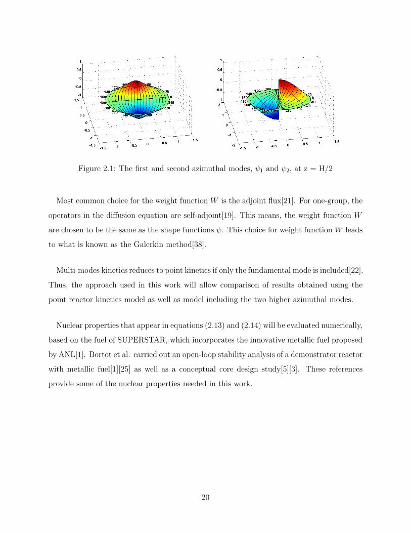
Figure 2.1: The first and second azimuthal modes, ψ1 and ψ2, at z = H/2

Most common choice for the weight function W is the adjoint flux[21]. For one-group, the

operators in the diffusion equation are self-adjoint[19]. This means, the weight function W

are chosen to be the same as the shape functions ψ. This choice for weight function W leads

to what is known as the Galerkin method[38].

Multi-modes kinetics reduces to point kinetics if only the fundamental mode is included[22].

Thus, the approach used in this work will allow comparison of results obtained using the

point reactor kinetics model as well as model including the two higher azimuthal modes.

Nuclear properties that appear in equations (2.13) and (2.14) will be evaluated numerically,

based on the fuel of SUPERSTAR, which incorporates the innovative metallic fuel proposed

by ANL[1]. Bortot et al. carried out an open-loop stability analysis of a demonstrator reactor

with metallic fuel[1][25] as well as a conceptual core design study[5][3]. These references

provide some of the nuclear properties needed in this work.

20

CHAPTER 3

THERMAL-HYDRAULICS USING A REDUCEDORDER MODEL

A reduced order model is used in this work for the thermal-hydraulics part of the system.

Consistent with the number of HXs, the reactor core is divided into 4 equal quadrants.

Depending on whether the HX model is coupled or not, the thermal-hydraulics models

either form a natural circulation system (closed loops); or a forced circulation system (heated

channels only). In the natural circulation system, each quadrant forms a closed equivalent

loop with its corresponding external pipes and HX. The driving force in the loop is induced

by the coolant density variation. The natural circulation system can be further divided into

two categories: the first is the natural circulation system without coupled neutronics, where

a constant heat generation rate represents the heat source term; the second is the natural

circulation system coupled with neutronics where the heat source is from fission reactions.

In the forced circulation system, constant pressure drop boundary conditions are applied on

heated channels in the reactor core. As in the natural circulation system without neutronics,

heat generation rate in the core is assumed to be constant. The fuel pin heat conduction

model is also developed in this chapter following the model in reference[9][31][32].

For the sake of simplicity, following assumptions are employed:

• Boussinesq approximation is valid and the coolant density variations are only caused by

temperature changes. Only the density in the gravity term in the momentum equation

is treated as time-dependent[30]. The equation of state describing this relation can be

found in reference[29].

• Heat generation rate in the fuel pellet along the z direction is uniform. In other words,

the fuel pellet and cladding temperature is assumed to vary only with the radial variable

21

r and time t. Furthermore, the coolant temperature in the heated channels is a function

of elevation z and time t, assuming well-mixed flow in the radial direction.

• Coolant temperature appearing in the fuel pin heat conduction model boundary con-

ditions is represented by a bulk temperature Tbulk(t) which is equal to the algorithmic

mean value of the coolant temperature at the inlet and the outlet of the core.

• Heat transfer process is only taking place in the reactor core heated channels and in

the HXs. The adiabatic boundary condition is applied on the pipes connecting them.

• Constant cross sectional area along the coolant flow path is assumed. For each equiv-

alent loop, there is only one coolant velocity for all segments.

• Friction at pressure drop for the whole loop (including the core and HXs) is represented

by a lumped friction factor. This factor is calculated at the nominal steady state of

the system.

• For the forced circulation case, in which fixed pressure drop boundary condition is

imposed across the core, the pressure drop in the reactor core is assumed to be one

half of the total pressure drop of the whole loop.

These assumptions reduce the complexity of the system considerably, and allow the de-

velopment of a reduced oeder model. Equations governing the coolant flow are developed

below.

3.1 Natural circulation model

In this section, both the steady state and time-dependent equations of the natural cir-

culation system are discussed. The steady state equations are simplified from their time-

dependent version, and their solutions also provide the initial conditions for their time-

dependent counterparts. Furthermore, the lumped friction factor is calculated from the

steady state momentum equation.

22

3.1.1 The time-dependent equations

• Continuity

u∗i (t) · A∗i = u∗j(t) · A∗j (3.1)

here, i and j represent cross sectional area at different positions along the flow path.

Due to strict constraint on the maximum velocity in the loop, the design is aimed at

keeping the cross sectional flow area nearly constant in the entire loop. Hence, based

on the assumption of constant cross sectional area along the coolant flow path, there

is only one u∗(t) and the continuity equation is satisfied at the outset.

• Conservation of momentum

For all segments in the loop, the frictional pressure drops are represented by a lumped

friction factor f ∗w

ρ∗(du∗

dt∗) = −∂p

∗

∂z∗+ ρ(z∗, t∗)g∗z + f ∗w ·

1

2· ρ∗ · (u∗)2 (3.2)

where ρ∗ is the average coolant density which is evaluated at the mean temperature

of the coolant at the core inlet and outlet under the nominal steady state. With

the reference length L∗ref , reference velocity v∗ref and the non-dimensional time t =

t∗/(L∗ref/v∗ref ), the dimensionless form of the equation above can be written as

du

dt= −∂p

∂z− ρ∗(z∗, t∗)

ρ∗gz − fw

1

2[u(t)]2 (3.3)

where, p = p∗

ρ∗(v∗ref )2, gz =

g∗zL∗ref

(v∗ref )2, fw = f ∗wL

∗ref . After rearranging, we have

−∂p∂z

=du

dt+ρ∗(z∗, t∗)

ρ∗gz + fw

1

2[u(t)]2 (3.4)

Figure 3.1 illustrates the coolant flow path in the primary loop. The lengths of the

horizontal pipes are exaggerated for the convenience of visualization. (Actually, SU-

PERSTAR incorporates integrated structure and its HXs are placed within the pres-

23

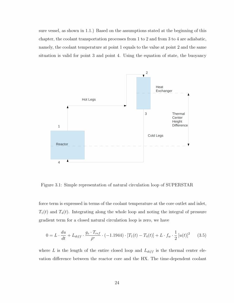
sure vessel, as shown in 1.1.) Based on the assumptions stated at the beginning of this

chapter, the coolant transportation processes from 1 to 2 and from 3 to 4 are adiabatic,

namely, the coolant temperature at point 1 equals to the value at point 2 and the same

situation is valid for point 3 and point 4. Using the equation of state, the buoyancy

4

1

3

2

Hot Legs

Cold Legs

Reactor

HeatExchanger

Thermal CenterHeightDifference

Figure 3.1: Simple representation of natural circulation loop of SUPERSTAR

force term is expressed in terms of the coolant temperature at the core outlet and inlet,

T1(t) and T4(t). Integrating along the whole loop and noting the integral of pressure

gradient term for a closed natural circulation loop is zero, we have

0 = L · dudt

+ Ldiff ·gz · Trefρ∗

· (−1.1944) · [T1(t)− T4(t)] + L · fw ·1

2[u(t)]2 (3.5)

where L is the length of the entire closed loop and Ldiff is the thermal center ele-

vation difference between the reactor core and the HX. The time-dependent coolant

24

temperature in the core is assumed to be a second order polynomial function of z

T (z, t) = Tci + a1(t)z + a2(t)z2 (3.6)

Evaluating at the core outlet, gives the time-dependent core exit temperature

T1(t) = Tco(t) = Tci + a1(t) ·H + a2(t) ·H2 (3.7)

The friction of pressure drop in the HXs is included in fw, and its energy transfer

characteristic is modeled as a first order polynomial

T4(t) = Tci(t) = p00 + p10 · Tco(t− τ1) + p01 · u(t− τ2) (3.8)

where p00, p10 and p01 are constants determined from the HX model, which is presented

later. τ1 is the time delay for the coolant to travel from point 1 to 4 in figure 3.1. τ2

accounts for the time delay for the coolant flow from point 2 to 4.

Finally, the momentum equation is written as a function of a1(t), a2(t) and u(t)

and their counterparts with time delays a1(t − τ1), a2(t − τ1) and u(t − τ2). The

momentum equation (3.5) for the natural circulation system is thus a delay differential

equation (DDE) for the independent variable u(t). Detailed derivation can be found

in Appendix D.

• Conservation of energy

For heated channels in the reactor core, the conservation of energy can be written as

ρ∗C∗p(∂T ∗

∂t∗+ u∗

∂T ∗

∂z∗) = k∗

∂2T ∗

∂(z∗)2+ q∗

′′′

e (3.9)

where ρ∗ is the average density evaluated at the average temperature of the reactor

core, k∗ and C∗p are also constants, evaluated at the average temperature. q∗′′′e is the

volumetric heat generation rate and it is an intermediate variable calculated from the

25

fuel pin conduction model. We have

q∗′′′

e = q∗′′ · P

∗

A∗(3.10)

where q∗′′

is the heat flux on the cladding surface, P ∗ is the wetted perimeter of a fuel

pin clad and A∗ is the cross sectional flow area associated with a fuel pin.

Earlier works on boiling water reactors[7][8] do not consider the heat conduction

effect in the coolant since conduction in water in BWR is negligible compared to

convection. However, thermal conductivity of liquid lead is much larger than that of

water. At 700 K, it is ∼ 17 Wm−1K−1. Thus, in equations (3.9) and later in (3.20),

the axial conduction term is retained. In order to capture the effect of conduction in

the solution of equation (3.9), we assume the coolant temperature in the hated channel

obeys a quadratic profile in z as in equation (3.6).

In order to reduce the space- and time-dependent PDEs to ODEs, Karve[7] and

Zhou[8] used a weighted residual procedure. Similar approach is used here to convert

equation (3.9) to ODEs variables a1(t) and a2(t). This procedure leads to

da1(t)

dt+ 2u(t)a2(t)− 6

H

[u(t) · a1(t)− 2αPba2(t)− P

Ah∞(Tc(rc, t)− Tbulk(t))

]= 0

(3.11)

and

da2(t)

dt− 6

H2

[u(t) · a1(t)− 2αPba2(t)− P


]= 0 (3.12)

where Tc(rc, t) is the cladding temperature which is evaluated at r = rc

Tc(r, t)|r=rc =Big

Big +Bic +BigBic log( rcrg

)Tp(rp, t)

+Bic


)Tbulk(t)

(3.13)

26

Tp(rp, t) and Tbulk(t) are intermediate variables which can be expressed in terms of

T0(t), T2(t), a1(t), a2(t), u(t) and their corresponding variations with delays. T0(t)

and T2(t) are variables from the fuel pin heat conduction model which are discussed

in section 3.3. Therefore, the conservation of coolant energy equation is described by

2 DDEs, equations (3.11) and (3.12). The complete derivation of these equations can

be found in Appendix E.

• Equation of State

ρ∗ = ρ∗(T ∗) = ρ∗(z∗, t∗) (3.14)

The equations of state of liquid lead are available in reference[22]. Within the range

of coolant temperature which is covered in transient scenarios in this work, the liquid

lead density can be approximately calculated by the equation:

ρ[kg/m3] = 11367− 1.1944 · T [K] (3.15)

So far, the development of the model for the coolant flow has focused on the heated chan-

nels. Next we expand the discussion to HXs, represented by equation (3.8). As mentioned

in the previous sections, the HXs play two roles in the system dynamics. One is the pressure

drop due to the frictional effect and the other is the energy transfer phenomena (sink). The

pressure drop over HXs has been integrated into the lumped friction factor, and hence, only

the heat transfer model needs to be considered. Because the detailed model for the HXs

incorporated in SUPERSTAR is not available yet, the energy transfer process is simulated

by a bilinear polynomial in two variables: the coolant temperature at the core outlet Tco(t),

and the coolant velocity u(t).

Recalling figure 3.1, the good here is to develop a model for the coolant temperature at

point 4, Tci(t), in terms of the coolant temperature at point 1 at some earlier time, Tco(t−τ1),

and the velocity at point 2 at some earlier time, u(t − τ2). (Because the finite velocity of

coolant transport in the loop, delay effects have to be included in this model.) These delay

effects render the original ODEs describing the SUPERSTAR system to be DDEs.

27

We assume that the energy transfer process in the HXs can be simulated by

Tci(t) = p00 + p10 · Tco(t− τ1) + p01 · u(t− τ2) (3.16)

where τ1 and τ2 are time delays which have the same physical meanings as in equation (3.8).

Although these time delays in general should be functions of the time-dependent coolant

velocity u(t), for the sake of simplicity, they are assumed to be constant in this work and

evaluated at the system nominal steady state. Tci(t) is the coolant temperature at the core

inlet at time t; Tco(t−τ1) is the coolant temperature at the core outlet at time t−τ1; u(t−τ2)

is the coolant velocity at the inlet of the HXs at time t−τ2. This polynomial equation relates

the core inlet temperature Tci(t) at time t with the core outlet temperature at time t − τ1

and the loop velocity at time t − τ2. p00, p10 and p01 are constants. The procedure to

determine these constants is described next. It is based on a quasi-static treatment of the

energy balance for the HXs.

For the energy balance in the HXs, we have

m · Cp ·∆T = Q (3.17)

where m is the mass flow rate in the HX; Cp is the heat capacity at the average coolant

temperature; ∆T = Tci(t)−Tco(t−τ1) and Q is the thermal energy flow rate. Here we assume

Q is a constant and equals to 75 MW, which is the nominal value for one heat exchanger.

This also corresponds to the scenario that even in transients on the reactor side, the power

conversion unit tries to extract a certain amount of heat to follow the external electric load.

The above equation can be further written as

ρ · u(t− τ2) · AHX · Cp · [Tci(t)− Tco(t− τ1)] = Q (3.18)

where ρ is the coolant density at the nominal steady state; u(t− τ2) is the coolant velocity;

AHX is the cross sectional area of the flow path in the HXs. The parameter AHX can be

found by setting the other parameters at their nominal steady state values, and then solving

28

this algebraic equation.

Now we have two independent variables, u(t − τ2) and Tco(t − τ1), and one dependent

variable Tci(t). In the context of quasi-steady state analysis, by setting one of the two

independent variables at its nominal value and varying the other one over a small range

close to its nominal value, we can get a set of values of Tci(t) (which forms a 3-D surface in

the space constructed by variables u(t− τ2), Tco(t− τ1) and Tci(t)).

To linearize the function of Tci with respect to Tco and u which is described by equation

(3.18), we assume that the energy transfer process in the HXs can be simulated by equation

(3.16).

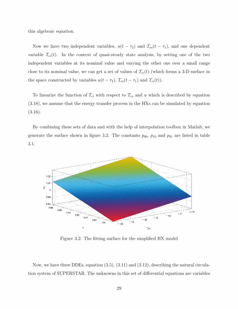
By combining these sets of data and with the help of interpolation toolbox in Matlab, we

generate the surface shown in figure 3.2. The constants p00, p10 and p01 are listed in table

3.1.

Figure 3.2: The fitting surface for the simplified HX model

Now, we have three DDEs, equation (3.5), (3.11) and (3.12), describing the natural circula-

tion system of SUPERSTAR. The unknowns in this set of differential equations are variables

29

Table 3.1: Constant coefficients in the simplified HX model

p00 0.1002p10 0.5237p01 0.4727

u(t), a1(t), a2(t) and variables from the heat conduction model. These differential equations

will be closed after they are coupled with the equations for T0(t) and T2(t) in section 3.3.

3.1.2 The steady state equations

The steady state equations are simplified from the time-dependent ones given earlier by

eliminating the time derivative term. And the same method as used earlier is used here to

reduce the PDEs to ODEs. Therefore, the derivation of these equations is not presented

here.

• Continuity

The assumption applied in the time-dependent formulation is valid here as well. There-

fore, for the steady state scenarios, only one u exists in each equivalent loop.

• Conservation of momentum

The conservation of momentum at the steady state is

∂p∗

∂z∗+ ρ(z∗)g∗z + f ∗w ·

1

2· ρ∗ · (u∗)2 = 0 (3.19)

The lumped friction factor f ∗w is determined by integrating the above equation along

the whole loop. The other parameters or properties are evaluated at the nominal state.

For the closed loop, the integral of the pressure gradient along the loop is zero, and the

friction-induced pressure drop is balanced by the buoyancy force due to the changes

in density. Thus, f ∗w can be solved from this equation.

The final form of the momentum equation is similar to its time-dependent counter-

part, except that there is no time derivative terms.

30

• Conservation of energy

For the heated channels in the reactor core

ρ∗C∗p(u∗dT ∗

dz∗) = k∗

d2T ∗

d(z∗)2+ q∗

′′′

e (3.20)

By assuming the coolant temperature has the same quadratic profile defined in equation

(3.6), this equation is reduced to two linear algebraic equations for a1 and a2 which

then can be solved. The results show that the value of the coefficient of the quadratic

term a2 is considerably small, and of the order of less than 10−6. That means, the

profile of coolant temperature is very close to linear. This is because the Pe number

in the heated channel is large (of the scale of 106), therefore, heat conduction along

the z direction can be omitted at the steady state, compared with convection.

The HX also runs at its nominal state. The HX coolant inlet and exit temperatures and

the coolant velocity are at their nominal values.

At the steady state, the time delay effect due to the coolant transport is not explicit any

more because the operation variables remain the same with respect to time. The system at its

steady state is described by a set of linear algebraic eqautions, and the steady state solutions

are obtained by solving these equations. The solutions of these steady state equations, are

the initial conditions for their time-dependent counterparts and also the starting points in

later transient analyses.

3.2 Forced circualtion model

The model for the forced circulation case only includes the core, with imposed pressure

drop boundary condition. Model for the rest of the loop is not necessary for forced circulation

case. Equations (3.1), (3.2) and (3.9) still apply. Equation (3.8) is not needed any more

because in the forced circulation system (open loop), Tci(t) is not a function of Tco(t) and

u(t) as it is set externally as an input.

31

The integral of the pressure gradient term over the core length in equation (3.2), ∆P ,

is specified as a boundary condition. In this study, it is assumed that both the reactor

core and the HXs account for one half of the total pressure drop along the whole loop.

This assumption is assumed valid at the steady state and during transients. In the previous

section, the total frictional pressure drop of the whole loop was found. The nominal pressure

drop across the core is one half of this value.

3.3 Fuel pin heat conduction model

The fuel for SUPERSTAR has not been selected yet, but one potential choice is the

innovative particulate-based metallic fuel[1][27]. Its heat conduction model can be derived

in a manner similar to that described in references[9][31][32]. The thermal and physical

properties of metallic fuel can be found in reference[26]. The weighted residual method

is used here to transform the heat conduction PDEs to ODEs as opposed to variational

approach used in reference[9].

The heat conduction equation of a fuel pellet and its cladding can be written[31] as:

ρ∗pC∗p

∂T ∗p (r∗, t∗)

∂t∗= k∗p

[∂2T ∗p (r∗, t∗)

∂r∗2+

1

r∗∂T ∗p (r∗, t∗)

∂r∗

]+ q∗

′′′

c (t) , 0 ≤ r∗ ≤ r∗p (3.21)

and

ρ∗cC∗c

∂T ∗c (r∗, t∗)

∂t∗= k∗c

[∂2T ∗c (r∗, t∗)

∂r∗2+

1

r∗∂T ∗c (r∗, t∗)

∂r∗

], r∗g ≤ r∗ ≤ r∗c (3.22)

with boundary conditions∂T ∗p (r∗, t∗)

∂r∗|r∗=0 = 0 (3.23)

−k∗p∂T ∗p (r∗p, t

∗)

∂r∗=r∗gr∗ph∗g[T ∗p (r∗p, t

∗)− T ∗c (r∗g , t∗)]

(3.24)

−k∗c∂T ∗c (r∗g , t

∗)

∂r∗= h∗g

[T ∗p (r∗p, t

∗)− T ∗c (r∗g , t∗)]

(3.25)

−k∗c∂T ∗c (r∗c , t

∗)

∂r∗= h∗∞ [T ∗c (r∗c , t

∗)− T ∗bulk(t)] (3.26)

32

The heat generation rate term q∗′′′c (t) can be expressed in terms of variables n0(t), n1(t) and

n2(t) from the neutronics model:

q∗′′′

c (t) = c∗qn∗0(t∗) + c∗qζ1n

∗1(t∗) + c∗qζ2n

∗2(t∗) (3.27)

c∗q, ζ1 and ζ2 are constants used in the fuel pin heat conduction model which are derived in

detail in Appendix C. Explanations for other symbols can be found in Appendix B. The

convective heat transfer coefficient h∗∞ is estimated by the Dittus-Boelter correlation

Nu = 0.023 ·Re0.8 · Pr0.4 (3.28)

where

Nu =h∗∞D

kPb(3.29)

and D is the equivalent diameter of the heated channel and kPb is the thermal conductivity

of coolant evaluated at the mean temperature.

The dimensionless form of the set of heat conduction equations above is

1

αp

∂Tp(r, t)

∂t=

[∂2Tp(r, t)

∂r2+

1

r

∂Tp(r, t)

∂r

]+cqn0(t)+cqζ1n1(t)+cqζ2n2(t), 0 ≤ r ≤ rp (3.30)

1

αc

∂Tc(r, t)

∂t=∂2Tc(r, t)

∂r2+

1

r

∂Tc(r, t)

∂r, rg ≤ r ≤ rc (3.31)

with boundary conditions∂Tp(r, t)

∂r|r=0 = 0 (3.32)

−∂Tp(rp, t)∂r

=Biprp

[Tp(rp, t)− Tc(rg, t)] (3.33)

−∂Tc(rg, t)∂r

=Bigrg

[Tp(rp, t)− Tc(rg, t)] (3.34)

−∂Tc(rc, t)∂r

=Bicrc

[Tc(rc, t)− Tbulk(t)] (3.35)

33

Retaining only the fundamental mode for the steady state, the corresponding steady state

conterparts for the above equations are:

0 =

[∂2Tp(r)

∂r2+

1

r

∂Tp(r)

∂r

]+ cqn0, 0 ≤ r ≤ rp (3.36)

0 =∂2Tc(r)

∂r2+

1

r

∂Tc(r)

∂r, rg ≤ r ≤ rc (3.37)

with boundary conditions

∂Tp(r)

∂r|r=0 = 0 (3.38)

−∂Tp(rp)∂r

=Biprp

[Tp(rp)− Tc(rg)

](3.39)

−∂Tc(rg)∂r

=Bigrg

[Tp(rp)− Tc(rg)

](3.40)

−∂Tc(rc)∂r

=Bicrc

[Tc(rc)− Tbulk

](3.41)

Solving equations (3.36–3.41), we have

Tp(r) = −cqn0r2

4+ b1, 0 ≤ r ≤ rp (3.42)

Tc(r) = b2 log(r) + b3, rg ≤ r ≤ rc (3.43)

where b2 and b3 are constants. The solutions of the steady state equations also form the

initial conditions for their time-dependent versions.

Realizing that the thermal diffusivity of the cladding α∗c is large relative to that of the

fuel, we can simplify equations (3.30) to (3.35) further. We first write the space- and time-

dependent variation of the clad temperature by making the constant coefficients in the

steady-state profile (equation 3.43) to be time-dependent

Tc(r, t) = b2(t) log(r) + b3(t), rg ≤ r ≤ rc (3.44)

34

and evaluating Tc(rg, t) in equation (3.32) in terms of Tp(rp, t) and Tbulk(t). Finally, we have

the strong form of the PDE

1

αp

∂Tp(r, t)

∂t=

[∂2Tp(r, t)

∂r2+

1

r

∂Tp(r, t)

∂r

]+cqn0(t)+cqζ1n1(t)+cqζ2n2(t), 0 ≤ r ≤ rp (3.45)


∂r|r=0 = 0 (3.46)

−∂Tp(rp, t)∂r

=Bi+prp

[Tp(rp, t)− Tbulk(t)] (3.47)

where Bi+p are the modified Biot number.

For a fuel pellet, its temperature at radial position r can be written as

Tp(r, t) = T0(t) + T2(t) · r2 (3.48)

where r is the radial coordinate with origin at the center line of the fuel pin. By using

the Weighted Residual Method, for each quadrant, two ODEs for coeffcients T0(t) and T2(t)

of the spatially-piecewise-quadratic function for the fuel pellet temperature are developed.

After rearranging, they are

1

αp

[dT0(t)

dtrp +

dT2(t)

dt

r3p

3

]− 4T2(t)rp − fArp − 2T2(t)rp − fB = 0 (3.49)

1

αp

[dT0(t)

dt

rp3

+dT2(t)

dt

r3p

5

]− 4T2(t)

rp3− fA

rp3− 2T2(t)rp − fB = 0 (3.50)

where

fA = cqn0(t) + cqζ1n1(t) + cqζ2n2(t) (3.51)

and

fB =Bi+prp

[Tp(rp, t)− Tbulk(t)] (3.52)

Additional details can be found in Appendix C.

35

CHAPTER 4

STABILITY ANALYSIS

There are three different systems studied in this work. First one is the natural circulation

system which has a nominal constant heat generation rate, and incorporates a simplified HX

model in the primary loop. Second is the forced circulation system comprised only of the core

which has a nominal constant heat generation rate, modeled by setting a constant pressure

drop boundary condition across the core. Third is the closed loop natural circulation system

coupled with neutronics and thermal-hydraulics. The stability analyses are carried out in

both frequency and time domain for the first two systems. For the third system, because

of the non-linear characteristics especially the feedback effects, the system is too large and

cumbersome, making the frequency domain analysis tremendously arduous. Therefore, only

time domain analyses are performed for the third system.

4.1 Natural circulation system without neutronics

This system is characterized by a constant heat generation rate in the core and a natural

circulation thermal-hydraulics model incorporating external pipes and HXs. Because the

velocity of the coolant is finite, the HX model in the loop introduces two time delays.

Therefore, this system is described by a set of DDEs. All four loops are identical, and hence

only one loop, consisting of five equations, is studied.

Frequency domain analyses

Stability analysis in the frequency domain for DDEs is different from that for ODEs

because of the effect of time lags. The time lags in the time domain change to exponential

terms in the frequency domain, thus making the equations transcendental. Rather than

36

a discrete set of eigenvalues (as is the case for finite number of ODEs), DDEs lead to a

continuous spectrum of eigenvalues[39]. Therefore, for the Jacobian matrix of DDEs, there

are infinite number of eigenvalues[39][40][41]. In this work, the DDE-BIFTOOL[42] is used to

carry out the stability analysis in the frequency domain. DDE-BIFTOOL “is a collection of

Matlab routines for numerical bifurcation analysis of systems of delay differential eqautions

with several fixed, discrete delays.[42]” The stability analysis codes will be used to evaluate

the eigenvalues whose real parts are larger than a finite real value.

As discussed in the previous chapters, for each equivalent channel in the thermal-hydraulics

part, there are five DDEs and five dependent variables (T0(t), T2(t), a1(t), a2(t), u(t)) (and

their counterparts with time delays). The steady state of this system is found by setting

the time-derivatives to zero and solving the resulting linear system. For the evaluation of

the eigenvalues, this system is found to be very stiff, leading to severe difficulties. It is

determined that the stiffness is due to the order of magnitude difference in the magnitudes

of variables a1 and a2, which are the coefficients of the linear and the quadratic terms in

the temperature profile (a2 � a1). This suggests that the profile is close to linear. Thus, to

reduce or eliminate the stiffness, the axial temperature profile is assumed to be linear, rather

than quadratic, thus eliminating a2(t). The fact that a2 at steady state is several orders of

magnitude smaller than a1, clearly suggests that ignoring the quadratic part that primarily

results from the conduction process is justified. (Peclet number of this system is also very

high, further justifying this step[37].)

The system is thus described by a set of four DDEs. With the nominal specifications[1], the

rightmost eigenvalues are evaluated using DDE-BIFTOOL, and plotted in Figure 4.1. The

rightmost pair of eigenvalues are −0.0061± 0.0891i. The frequency or period is determined

by the magnitude of the imaginary part of the rightmost eigenvalue,

2π

T= 0.0891 =⇒ T = 70.52 seconds (4.1)

37

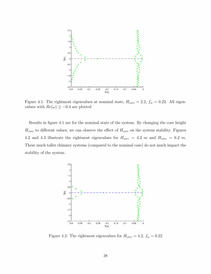
Figure 4.1: The rightmost eigenvalues at nominal state, Hcore = 2.2, fw = 0.22. All eigen-values with Re(ω) ≥ −0.4 are plotted

Results in figure 4.1 are for the nominal state of the system. By changing the core height

Hcore to different values, we can observe the effect of Hcore on the system stability. Figures

4.2 and 4.3 illustrate the rightmost eigenvalues for Hcore = 4.2 m and Hcore = 6.2 m.

These much taller chimney systems (compared to the nominal case) do not much impact the

stability of the system.

Figure 4.2: The rightmost eigenvalues for Hcore = 4.2, fw = 0.22

38

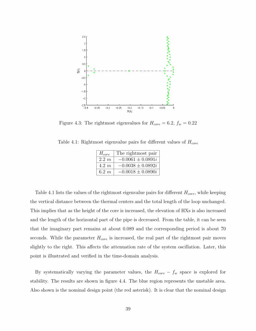
Figure 4.3: The rightmost eigenvalues for Hcore = 6.2, fw = 0.22

Table 4.1: Rightmost eigenvalue pairs for different values of Hcore

Hcore The rightmost pair2.2 m −0.0061± 0.0891i4.2 m −0.0038± 0.0892i6.2 m −0.0018± 0.0890i

Table 4.1 lists the values of the rightmost eigenvalue pairs for different Hcore, while keeping

the vertical distance between the thermal centers and the total length of the loop unchanged.

This implies that as the height of the core is increased, the elevation of HXs is also increased

and the length of the horizontal part of the pipe is decreased. From the table, it can be seen

that the imaginary part remains at about 0.089 and the corresponding period is about 70

seconds. While the parameter Hcore is increased, the real part of the rightmost pair moves

slightly to the right. This affects the attenuation rate of the system oscillation. Later, this

point is illustrated and verified in the time-domain analysis.

By systematically varying the parameter values, the Hcore − fw space is explored for

stability. The results are shown in figure 4.4. The blue region represents the unstable area.

Also shown is the nominal design point (the red asterisk). It is clear that the nominal design

39

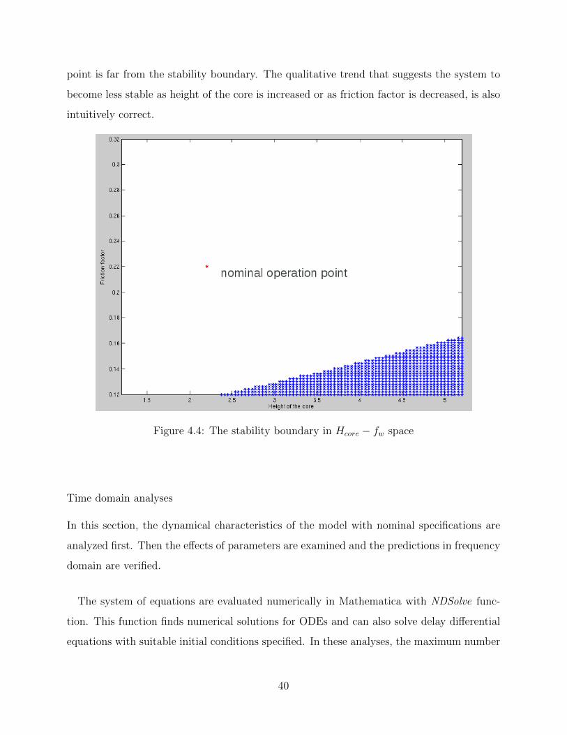
point is far from the stability boundary. The qualitative trend that suggests the system to

become less stable as height of the core is increased or as friction factor is decreased, is also

intuitively correct.

Figure 4.4: The stability boundary in Hcore − fw space

Time domain analyses

In this section, the dynamical characteristics of the model with nominal specifications are

analyzed first. Then the effects of parameters are examined and the predictions in frequency

domain are verified.

The system of equations are evaluated numerically in Mathematica with NDSolve func-

tion. This function finds numerical solutions for ODEs and can also solve delay differential

equations with suitable initial conditions specified. In these analyses, the maximum number

40

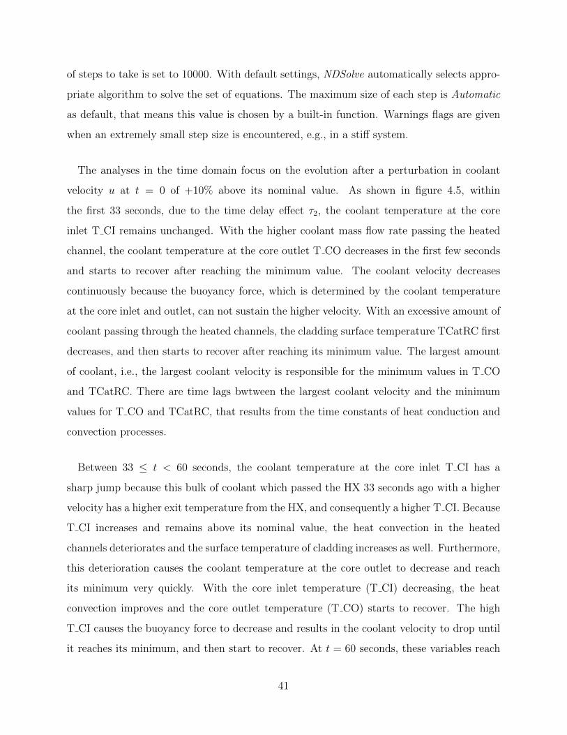
of steps to take is set to 10000. With default settings, NDSolve automatically selects appro-

priate algorithm to solve the set of equations. The maximum size of each step is Automatic

as default, that means this value is chosen by a built-in function. Warnings flags are given

when an extremely small step size is encountered, e.g., in a stiff system.

The analyses in the time domain focus on the evolution after a perturbation in coolant

velocity u at t = 0 of +10% above its nominal value. As shown in figure 4.5, within

the first 33 seconds, due to the time delay effect τ2, the coolant temperature at the core

inlet T CI remains unchanged. With the higher coolant mass flow rate passing the heated

channel, the coolant temperature at the core outlet T CO decreases in the first few seconds

and starts to recover after reaching the minimum value. The coolant velocity decreases

continuously because the buoyancy force, which is determined by the coolant temperature

at the core inlet and outlet, can not sustain the higher velocity. With an excessive amount of

coolant passing through the heated channels, the cladding surface temperature TCatRC first

decreases, and then starts to recover after reaching its minimum value. The largest amount

of coolant, i.e., the largest coolant velocity is responsible for the minimum values in T CO

and TCatRC. There are time lags bwtween the largest coolant velocity and the minimum

values for T CO and TCatRC, that results from the time constants of heat conduction and

convection processes.

Between 33 ≤ t < 60 seconds, the coolant temperature at the core inlet T CI has a

sharp jump because this bulk of coolant which passed the HX 33 seconds ago with a higher

velocity has a higher exit temperature from the HX, and consequently a higher T CI. Because

T CI increases and remains above its nominal value, the heat convection in the heated

channels deteriorates and the surface temperature of cladding increases as well. Furthermore,

this deterioration causes the coolant temperature at the core outlet to decrease and reach

its minimum very quickly. With the core inlet temperature (T CI) decreasing, the heat

convection improves and the core outlet temperature (T CO) starts to recover. The high

T CI causes the buoyancy force to decrease and results in the coolant velocity to drop until

it reaches its minimum, and then start to recover. At t = 60 seconds, these variables reach

41

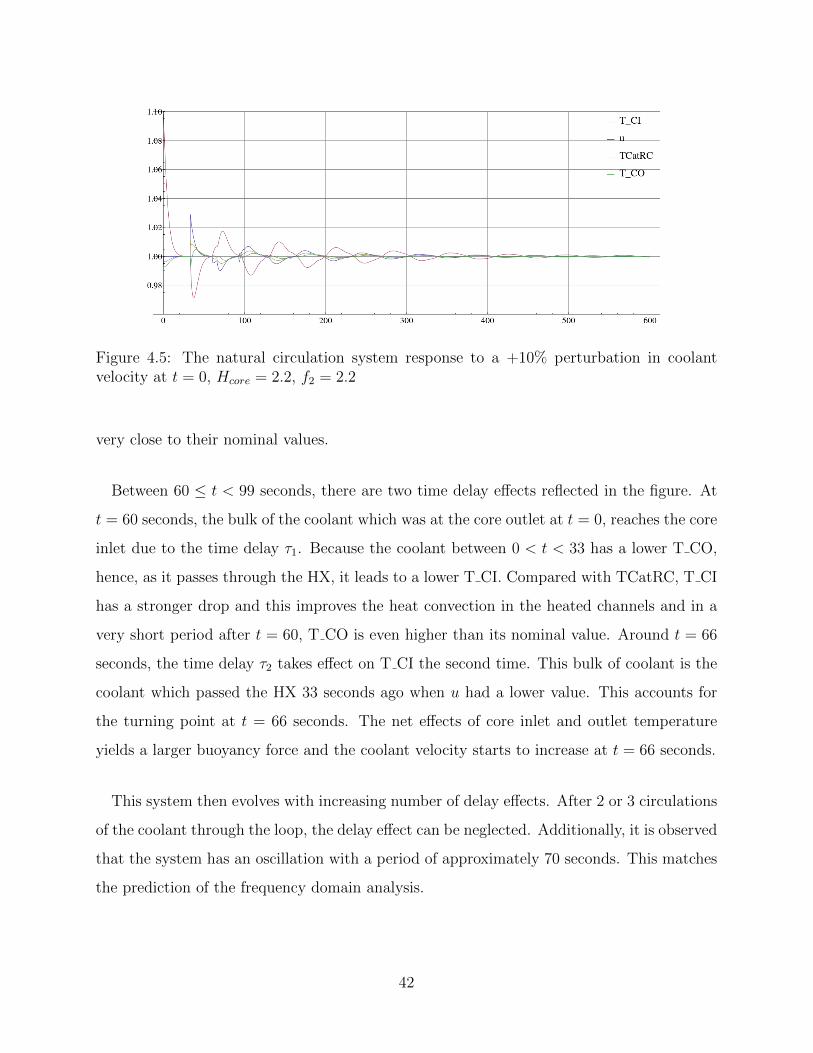
Figure 4.5: The natural circulation system response to a +10% perturbation in coolantvelocity at t = 0, Hcore = 2.2, f2 = 2.2

very close to their nominal values.

Between 60 ≤ t < 99 seconds, there are two time delay effects reflected in the figure. At

t = 60 seconds, the bulk of the coolant which was at the core outlet at t = 0, reaches the core

inlet due to the time delay τ1. Because the coolant between 0 < t < 33 has a lower T CO,

hence, as it passes through the HX, it leads to a lower T CI. Compared with TCatRC, T CI

has a stronger drop and this improves the heat convection in the heated channels and in a

very short period after t = 60, T CO is even higher than its nominal value. Around t = 66

seconds, the time delay τ2 takes effect on T CI the second time. This bulk of coolant is the

coolant which passed the HX 33 seconds ago when u had a lower value. This accounts for

the turning point at t = 66 seconds. The net effects of core inlet and outlet temperature

yields a larger buoyancy force and the coolant velocity starts to increase at t = 66 seconds.

This system then evolves with increasing number of delay effects. After 2 or 3 circulations

of the coolant through the loop, the delay effect can be neglected. Additionally, it is observed

that the system has an oscillation with a period of approximately 70 seconds. This matches

the prediction of the frequency domain analysis.

42

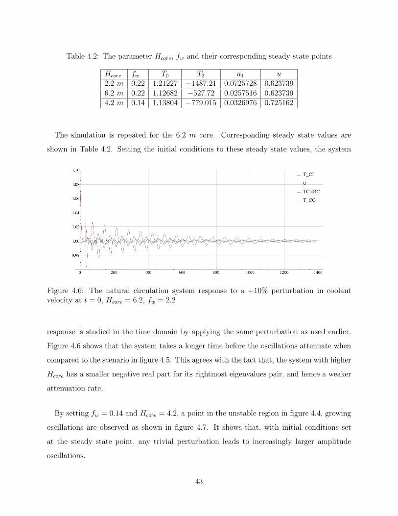
Table 4.2: The parameter Hcore, fw and their corresponding steady state points

Hcore fw T0 T2 a1 u2.2 m 0.22 1.21227 −1487.21 0.0725728 0.6237396.2 m 0.22 1.12682 −527.72 0.0257516 0.6237394.2 m 0.14 1.13804 −779.015 0.0326976 0.725162

The simulation is repeated for the 6.2 m core. Corresponding steady state values are

shown in Table 4.2. Setting the initial conditions to these steady state values, the system

Figure 4.6: The natural circulation system response to a +10% perturbation in coolantvelocity at t = 0, Hcore = 6.2, fw = 2.2

response is studied in the time domain by applying the same perturbation as used earlier.

Figure 4.6 shows that the system takes a longer time before the oscillations attenuate when

compared to the scenario in figure 4.5. This agrees with the fact that, the system with higher

Hcore has a smaller negative real part for its rightmost eigenvalues pair, and hence a weaker

attenuation rate.

By setting fw = 0.14 and Hcore = 4.2, a point in the unstable region in figure 4.4, growing

oscillations are observed as shown in figure 4.7. It shows that, with initial conditions set

at the steady state point, any trivial perturbation leads to increasingly larger amplitude

oscillations.

43

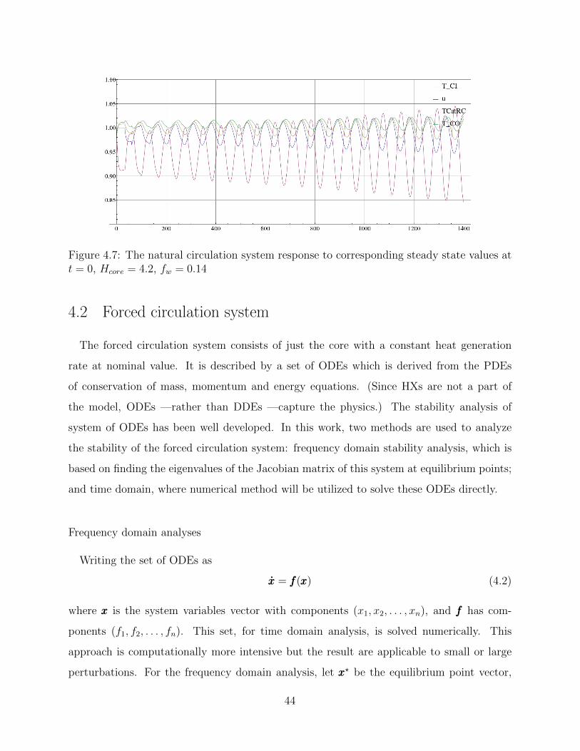
Figure 4.7: The natural circulation system response to corresponding steady state values att = 0, Hcore = 4.2, fw = 0.14

4.2 Forced circulation system

The forced circulation system consists of just the core with a constant heat generation

rate at nominal value. It is described by a set of ODEs which is derived from the PDEs

of conservation of mass, momentum and energy equations. (Since HXs are not a part of

the model, ODEs —rather than DDEs —capture the physics.) The stability analysis of

system of ODEs has been well developed. In this work, two methods are used to analyze

the stability of the forced circulation system: frequency domain stability analysis, which is

based on finding the eigenvalues of the Jacobian matrix of this system at equilibrium points;

and time domain, where numerical method will be utilized to solve these ODEs directly.

Frequency domain analyses

Writing the set of ODEs as

xxx = fff(xxx) (4.2)

where xxx is the system variables vector with components (x1, x2, . . . , xn), and fff has com-

ponents (f1, f2, . . . , fn). This set, for time domain analysis, is solved numerically. This

approach is computationally more intensive but the result are applicable to small or large

perturbations. For the frequency domain analysis, let xxx? be the equilibrium point vector,

44

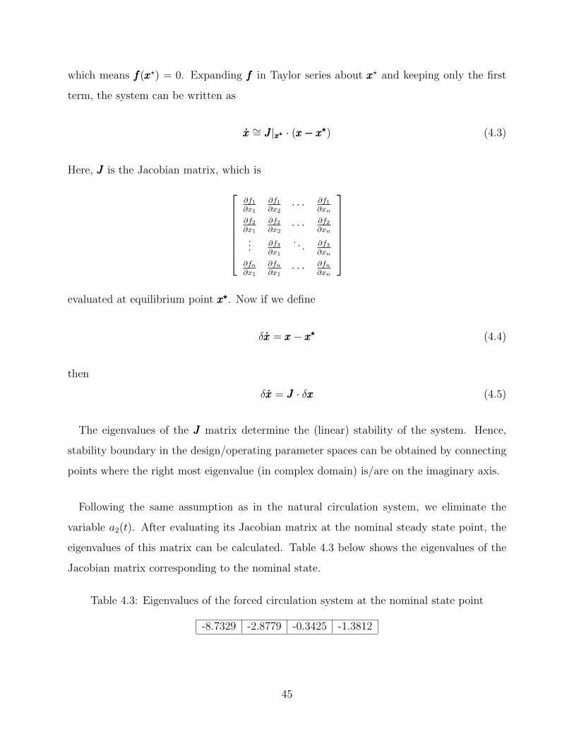
which means fff(xxx?) = 0. Expanding fff in Taylor series about xxx? and keeping only the first

term, the system can be written as

xxx ∼= JJJ |x?x?x? · (x− x?x− x?x− x?) (4.3)

Here, JJJ is the Jacobian matrix, which is

∂f1∂x1

∂f1∂x2

· · · ∂f1∂xn

∂f2∂x1

∂f2∂x2

· · · ∂f2∂xn

... ∂f3∂x1

. . . ∂f3∂xn

∂fn∂x1

∂fn∂x1

· · · ∂fn∂xn

evaluated at equilibrium point x?x?x?. Now if we define

δxxx = xxx− x?x?x? (4.4)

then

δxxx = JJJ · δxxx (4.5)

The eigenvalues of the JJJ matrix determine the (linear) stability of the system. Hence,

stability boundary in the design/operating parameter spaces can be obtained by connecting

points where the right most eigenvalue (in complex domain) is/are on the imaginary axis.

Following the same assumption as in the natural circulation system, we eliminate the

variable a2(t). After evaluating its Jacobian matrix at the nominal steady state point, the

eigenvalues of this matrix can be calculated. Table 4.3 below shows the eigenvalues of the

Jacobian matrix corresponding to the nominal state.

Table 4.3: Eigenvalues of the forced circulation system at the nominal state point

-8.7329 -2.8779 -0.3425 -1.3812

45

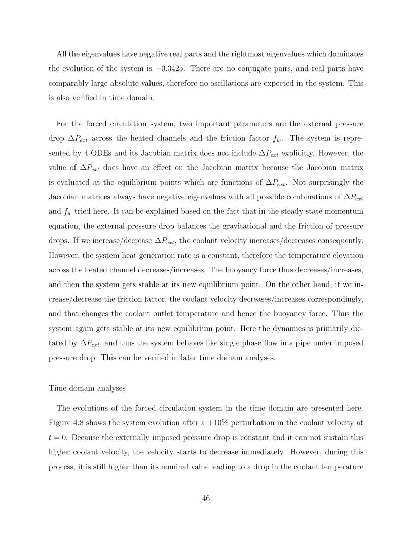
All the eigenvalues have negative real parts and the rightmost eigenvalues which dominates

the evolution of the system is −0.3425. There are no conjugate pairs, and real parts have

comparably large absolute values, therefore no oscillations are expected in the system. This

is also verified in time domain.

For the forced circulation system, two important parameters are the external pressure

drop ∆Pext across the heated channels and the friction factor fw. The system is repre-

sented by 4 ODEs and its Jacobian matrix does not include ∆Pext explicitly. However, the

value of ∆Pext does have an effect on the Jacobian matrix because the Jacobian matrix

is evaluated at the equilibrium points which are functions of ∆Pext. Not surprisingly the

Jacobian matrices always have negative eigenvalues with all possible combinations of ∆Pext

and fw tried here. It can be explained based on the fact that in the steady state momentum

equation, the external pressure drop balances the gravitational and the friction of pressure

drops. If we increase/decrease ∆Pext, the coolant velocity increases/decreases consequently.

However, the system heat generation rate is a constant, therefore the temperature elevation

across the heated channel decreases/increases. The buoyancy force thus decreases/increases,

and then the system gets stable at its new equilibrium point. On the other hand, if we in-

crease/decrease the friction factor, the coolant velocity decreases/increases correspondingly,

and that changes the coolant outlet temperature and hence the buoyancy force. Thus the

system again gets stable at its new equilibrium point. Here the dynamics is primarily dic-

tated by ∆Pext, and thus the system behaves like single phase flow in a pipe under imposed

pressure drop. This can be verified in later time domain analyses.

Time domain analyses

The evolutions of the forced circulation system in the time domain are presented here.

Figure 4.8 shows the system evolution after a +10% perturbation in the coolant velocity at

t = 0. Because the externally imposed pressure drop is constant and it can not sustain this

higher coolant velocity, the velocity starts to decrease immediately. However, during this

process, it is still higher than its nominal value leading to a drop in the coolant temperature

46

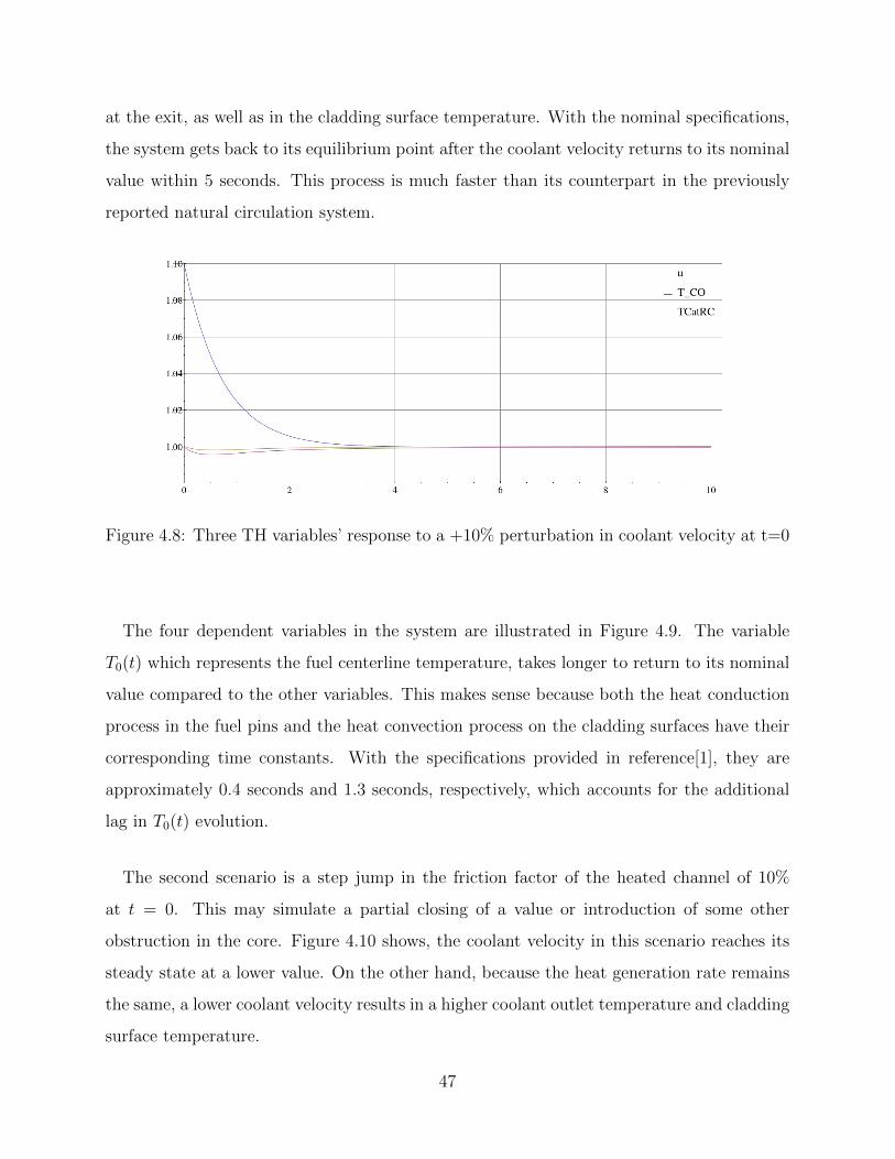
at the exit, as well as in the cladding surface temperature. With the nominal specifications,

the system gets back to its equilibrium point after the coolant velocity returns to its nominal

value within 5 seconds. This process is much faster than its counterpart in the previously

reported natural circulation system.

Figure 4.8: Three TH variables’ response to a +10% perturbation in coolant velocity at t=0

The four dependent variables in the system are illustrated in Figure 4.9. The variable

T0(t) which represents the fuel centerline temperature, takes longer to return to its nominal

value compared to the other variables. This makes sense because both the heat conduction

process in the fuel pins and the heat convection process on the cladding surfaces have their

corresponding time constants. With the specifications provided in reference[1], they are

approximately 0.4 seconds and 1.3 seconds, respectively, which accounts for the additional

lag in T0(t) evolution.

The second scenario is a step jump in the friction factor of the heated channel of 10%

at t = 0. This may simulate a partial closing of a value or introduction of some other

obstruction in the core. Figure 4.10 shows, the coolant velocity in this scenario reaches its

steady state at a lower value. On the other hand, because the heat generation rate remains

the same, a lower coolant velocity results in a higher coolant outlet temperature and cladding

surface temperature.

47

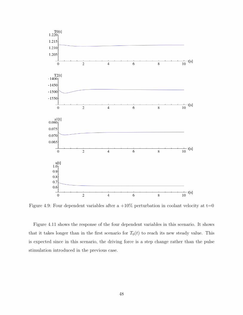
Figure 4.9: Four dependent variables after a +10% perturbation in coolant velocity at t=0

Figure 4.11 shows the response of the four dependent variables in this scenario. It shows

that it takes longer than in the first scenario for T0(t) to reach its new steady value. This

is expected since in this scenario, the driving force is a step change rather than the pulse

stimulation introduced in the previous case.

48

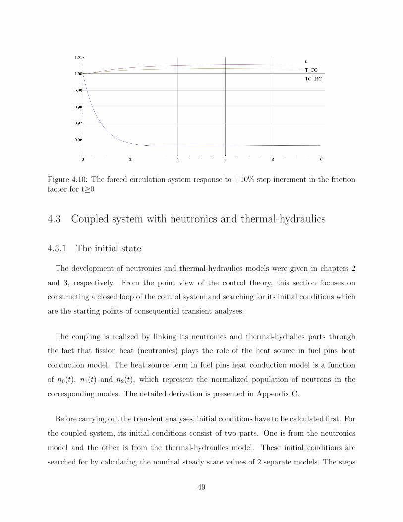
Figure 4.10: The forced circulation system response to +10% step increment in the frictionfactor for t≥0

4.3 Coupled system with neutronics and thermal-hydraulics

4.3.1 The initial state

The development of neutronics and thermal-hydraulics models were given in chapters 2

and 3, respectively. From the point view of the control theory, this section focuses on

constructing a closed loop of the control system and searching for its initial conditions which

are the starting points of consequential transient analyses.

The coupling is realized by linking its neutronics and thermal-hydralics parts through

the fact that fission heat (neutronics) plays the role of the heat source in fuel pins heat

conduction model. The heat source term in fuel pins heat conduction model is a function

of n0(t), n1(t) and n2(t), which represent the normalized population of neutrons in the

corresponding modes. The detailed derivation is presented in Appendix C.

Before carrying out the transient analyses, initial conditions have to be calculated first. For

the coupled system, its initial conditions consist of two parts. One is from the neutronics

model and the other is from the thermal-hydraulics model. These initial conditions are

searched for by calculating the nominal steady state values of 2 separate models. The steps

49

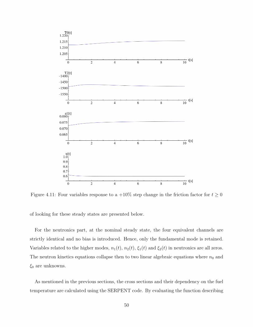
Figure 4.11: Four variables response to a +10% step change in the friction factor for t ≥ 0

of looking for these steady states are presented below.

For the neutronics part, at the nominal steady state, the four equivalent channels are

strictly identical and no bias is introduced. Hence, only the fundamental mode is retained.

Variables related to the higher modes, n1(t), n2(t), ξ1(t) and ξ2(t) in neutronics are all zeros.

The neutron kinetics equations collapse then to two linear algebraic equations where n0 and

ξ0 are unknowns.

As mentioned in the previous sections, the cross sections and their dependency on the fuel

temperature are calculated using the SERPENT code. By evaluating the function describing

50

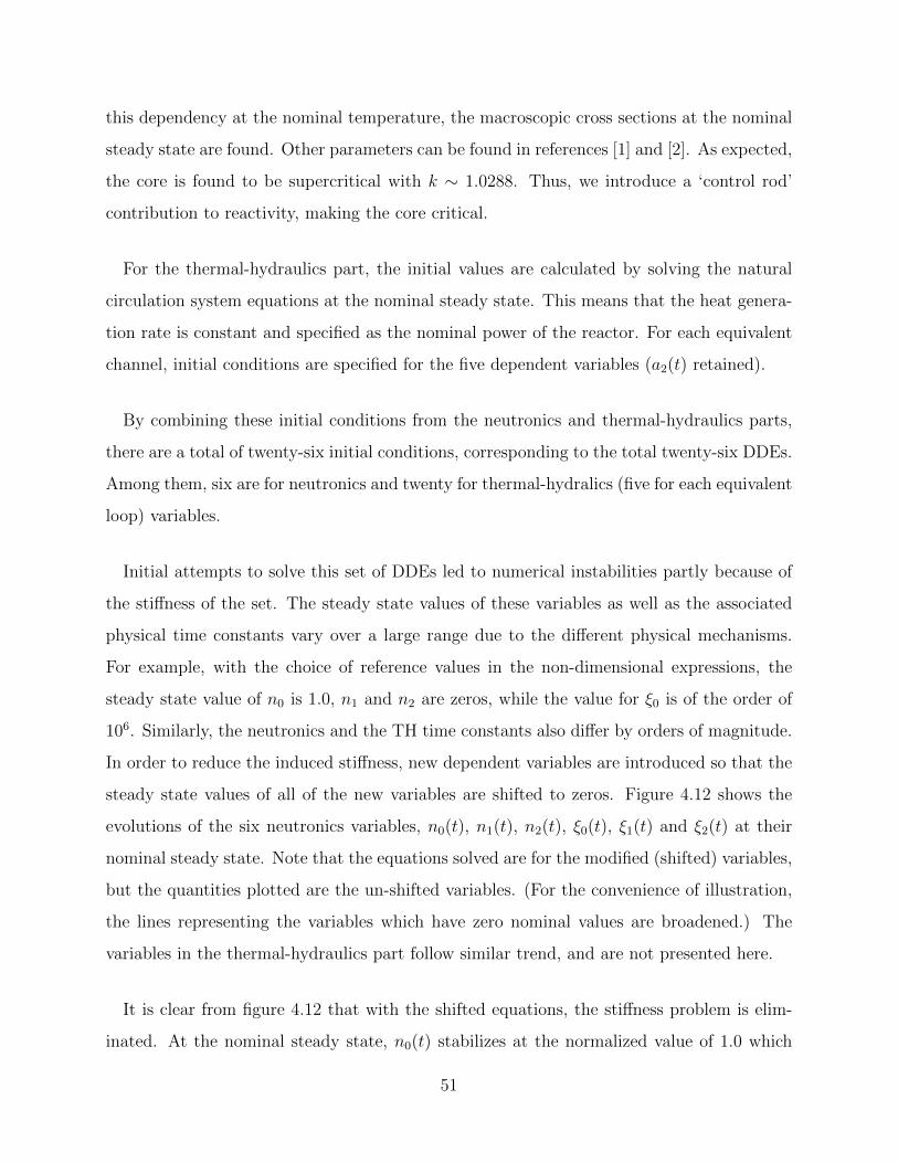
this dependency at the nominal temperature, the macroscopic cross sections at the nominal

steady state are found. Other parameters can be found in references [1] and [2]. As expected,

the core is found to be supercritical with k ∼ 1.0288. Thus, we introduce a ‘control rod’

contribution to reactivity, making the core critical.

For the thermal-hydraulics part, the initial values are calculated by solving the natural

circulation system equations at the nominal steady state. This means that the heat genera-

tion rate is constant and specified as the nominal power of the reactor. For each equivalent

channel, initial conditions are specified for the five dependent variables (a2(t) retained).

By combining these initial conditions from the neutronics and thermal-hydraulics parts,

there are a total of twenty-six initial conditions, corresponding to the total twenty-six DDEs.

Among them, six are for neutronics and twenty for thermal-hydralics (five for each equivalent

loop) variables.

Initial attempts to solve this set of DDEs led to numerical instabilities partly because of

the stiffness of the set. The steady state values of these variables as well as the associated

physical time constants vary over a large range due to the different physical mechanisms.

For example, with the choice of reference values in the non-dimensional expressions, the

steady state value of n0 is 1.0, n1 and n2 are zeros, while the value for ξ0 is of the order of

106. Similarly, the neutronics and the TH time constants also differ by orders of magnitude.

In order to reduce the induced stiffness, new dependent variables are introduced so that the

steady state values of all of the new variables are shifted to zeros. Figure 4.12 shows the

evolutions of the six neutronics variables, n0(t), n1(t), n2(t), ξ0(t), ξ1(t) and ξ2(t) at their

nominal steady state. Note that the equations solved are for the modified (shifted) variables,

but the quantities plotted are the un-shifted variables. (For the convenience of illustration,

the lines representing the variables which have zero nominal values are broadened.) The

variables in the thermal-hydraulics part follow similar trend, and are not presented here.

It is clear from figure 4.12 that with the shifted equations, the stiffness problem is elim-

inated. At the nominal steady state, n0(t) stabilizes at the normalized value of 1.0 which

51

Figure 4.12: Neutronics variables at the nominal steady state

corresponds to the 100% power level. At the steady state, the amplitude of the first and

second modes, n1(t) and n2(t) are zero, because the four equivalent channels are strictly

identical and no bias in neutronics is introduced at the nominal state. The normalized con-

centrations of delayed neutron precursor for each mode are represented by ξ0(t), ξ1(t) and

ξ2(t). It is illustrated that, the concentration of delayed neutron precursor caused by the

fundamental mode remains at its steady value, while the higher modes at the nominal state

52

are at zero value.

In the thermal-hydraulics model, there are five variables for each equivalent channel,

namely, T0,q(t), T2,q(t), a1,q(t), a2,q(t) and uq(t). Here, the subscript q represents the quadrant

number. Because all four channels are equal at this nominal steady state, for simplicity, q is

omitted in this section. Figure 4.13 shows the 5 variables in quadrant number 1. Because the

nominal value of a2(t) is very close to zero, the line representing this variable is broadened

for better illustration.

Thus, for all twenty-six variables, the steady state values have been found, and these form

the starting points (initial conditions) for later transient analyses.

4.3.2 The time domain analysis

As for the time domain analyses reported in previous section, Mathematica’s NDSolve

function is used to integrate the set of DDEs numerically. Eight scenarios are simulated.

They are:

1. control rod induced negative reactivity (13 cents) in quadrant number 2 at t = 0

2. control rod induced negative reactivity (13 cents for each quadrant) in quadrants 2

and 3 at t = 0

3. control rod induced positive reactivity (13 cents for each quadrant) in quadrants 2 and

3 at t = 0

4. a case showing prompt criticality

5. friction factor variation (Tripled) in quadrants 2 and 3 at t ≥ 0 (simulating a blockage)

6. inlet temperature variation between 5 ≤ t ≤ 15 (simulating a malfunctioning HX)

7. comparison between the multi-modes and the fundamental mode ‘point’ kinetics

8. effects of different time delay constants

53

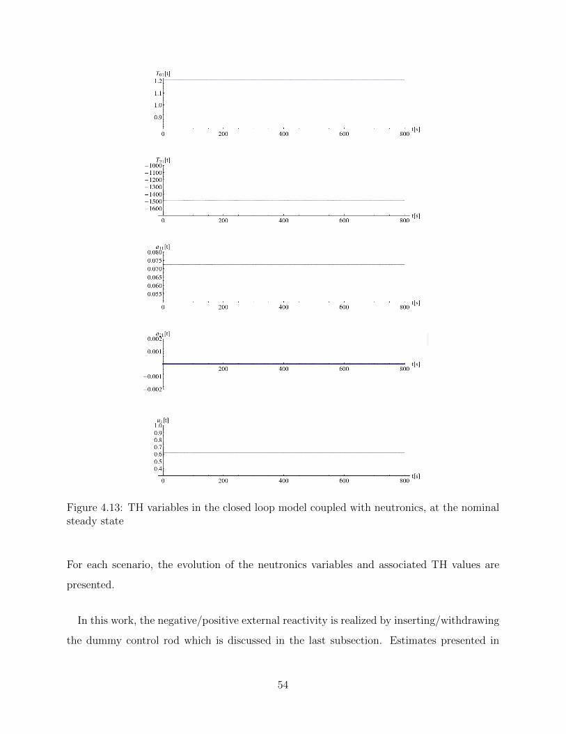
Figure 4.13: TH variables in the closed loop model coupled with neutronics, at the nominalsteady state

For each scenario, the evolution of the neutronics variables and associated TH values are

presented.

In this work, the negative/positive external reactivity is realized by inserting/withdrawing

the dummy control rod which is discussed in the last subsection. Estimates presented in

54

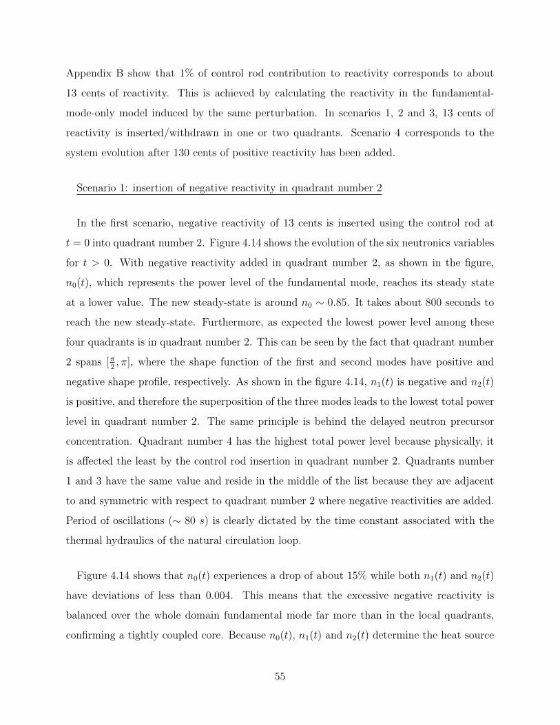
Appendix B show that 1% of control rod contribution to reactivity corresponds to about

13 cents of reactivity. This is achieved by calculating the reactivity in the fundamental-

mode-only model induced by the same perturbation. In scenarios 1, 2 and 3, 13 cents of

reactivity is inserted/withdrawn in one or two quadrants. Scenario 4 corresponds to the

system evolution after 130 cents of positive reactivity has been added.

Scenario 1: insertion of negative reactivity in quadrant number 2

In the first scenario, negative reactivity of 13 cents is inserted using the control rod at

t = 0 into quadrant number 2. Figure 4.14 shows the evolution of the six neutronics variables

for t > 0. With negative reactivity added in quadrant number 2, as shown in the figure,

n0(t), which represents the power level of the fundamental mode, reaches its steady state

at a lower value. The new steady-state is around n0 ∼ 0.85. It takes about 800 seconds to

reach the new steady-state. Furthermore, as expected the lowest power level among these

four quadrants is in quadrant number 2. This can be seen by the fact that quadrant number

2 spans [π2, π], where the shape function of the first and second modes have positive and

negative shape profile, respectively. As shown in the figure 4.14, n1(t) is negative and n2(t)

is positive, and therefore the superposition of the three modes leads to the lowest total power

level in quadrant number 2. The same principle is behind the delayed neutron precursor

concentration. Quadrant number 4 has the highest total power level because physically, it

is affected the least by the control rod insertion in quadrant number 2. Quadrants number

1 and 3 have the same value and reside in the middle of the list because they are adjacent

to and symmetric with respect to quadrant number 2 where negative reactivities are added.

Period of oscillations (∼ 80 s) is clearly dictated by the time constant associated with the

thermal hydraulics of the natural circulation loop.

Figure 4.14 shows that n0(t) experiences a drop of about 15% while both n1(t) and n2(t)

have deviations of less than 0.004. This means that the excessive negative reactivity is

balanced over the whole domain fundamental mode far more than in the local quadrants,

confirming a tightly coupled core. Because n0(t), n1(t) and n2(t) determine the heat source

55

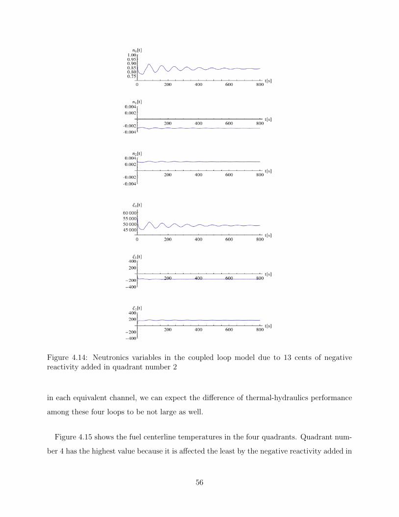
Figure 4.14: Neutronics variables in the coupled loop model due to 13 cents of negativereactivity added in quadrant number 2

in each equivalent channel, we can expect the difference of thermal-hydraulics performance

among these four loops to be not large as well.

Figure 4.15 shows the fuel centerline temperatures in the four quadrants. Quadrant num-

ber 4 has the highest value because it is affected the least by the negative reactivity added in

56

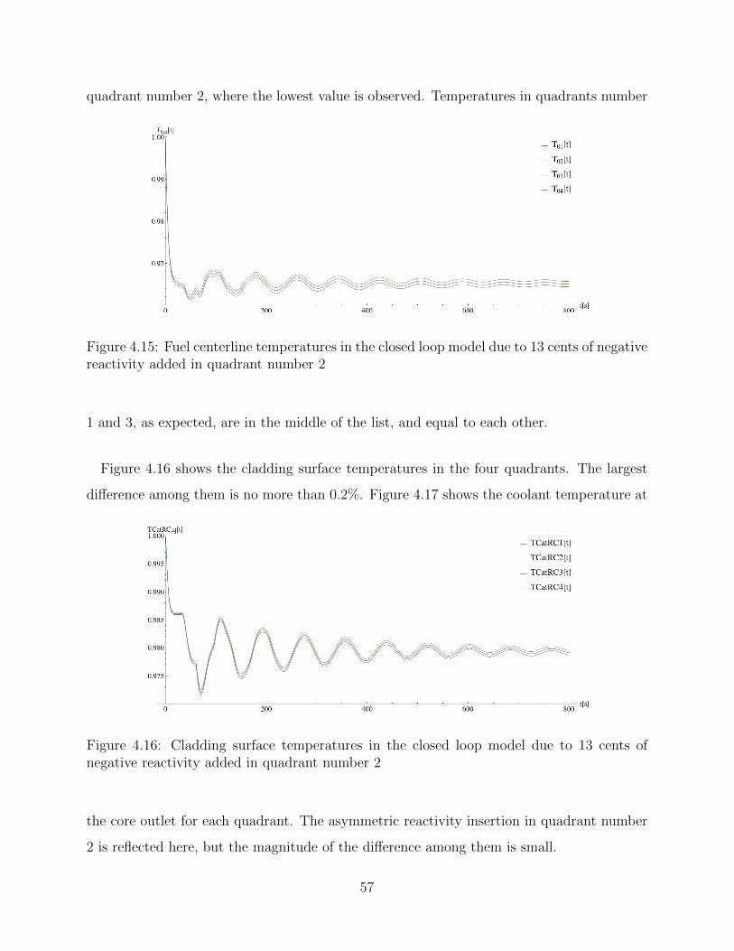
quadrant number 2, where the lowest value is observed. Temperatures in quadrants number

Figure 4.15: Fuel centerline temperatures in the closed loop model due to 13 cents of negativereactivity added in quadrant number 2

1 and 3, as expected, are in the middle of the list, and equal to each other.

Figure 4.16 shows the cladding surface temperatures in the four quadrants. The largest

difference among them is no more than 0.2%. Figure 4.17 shows the coolant temperature at

Figure 4.16: Cladding surface temperatures in the closed loop model due to 13 cents ofnegative reactivity added in quadrant number 2

the core outlet for each quadrant. The asymmetric reactivity insertion in quadrant number

2 is reflected here, but the magnitude of the difference among them is small.

57

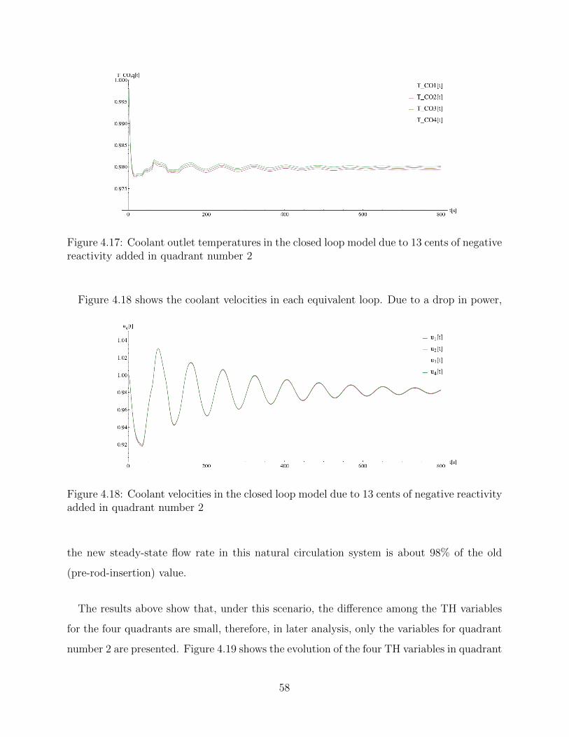
Figure 4.17: Coolant outlet temperatures in the closed loop model due to 13 cents of negativereactivity added in quadrant number 2

Figure 4.18 shows the coolant velocities in each equivalent loop. Due to a drop in power,

Figure 4.18: Coolant velocities in the closed loop model due to 13 cents of negative reactivityadded in quadrant number 2

the new steady-state flow rate in this natural circulation system is about 98% of the old

(pre-rod-insertion) value.

The results above show that, under this scenario, the difference among the TH variables

for the four quadrants are small, therefore, in later analysis, only the variables for quadrant

number 2 are presented. Figure 4.19 shows the evolution of the four TH variables in quadrant

58

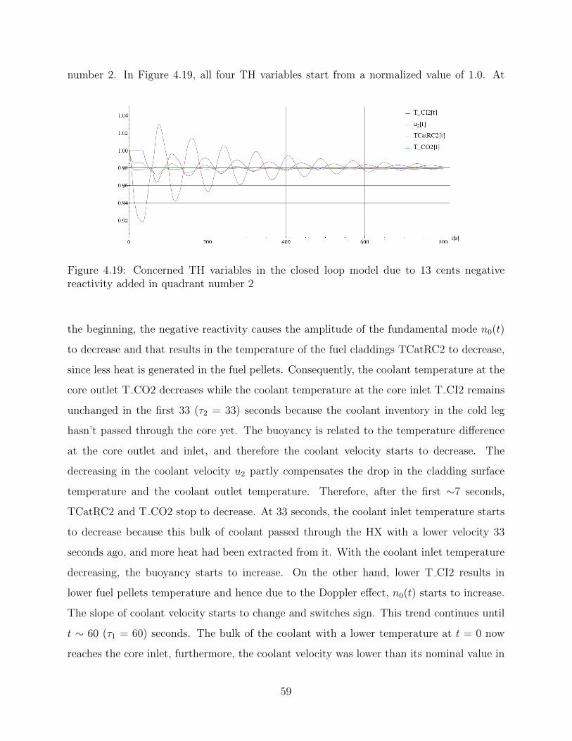
number 2. In Figure 4.19, all four TH variables start from a normalized value of 1.0. At

Figure 4.19: Concerned TH variables in the closed loop model due to 13 cents negativereactivity added in quadrant number 2

the beginning, the negative reactivity causes the amplitude of the fundamental mode n0(t)

to decrease and that results in the temperature of the fuel claddings TCatRC2 to decrease,

since less heat is generated in the fuel pellets. Consequently, the coolant temperature at the

core outlet T CO2 decreases while the coolant temperature at the core inlet T CI2 remains

unchanged in the first 33 (τ2 = 33) seconds because the coolant inventory in the cold leg

hasn’t passed through the core yet. The buoyancy is related to the temperature difference

at the core outlet and inlet, and therefore the coolant velocity starts to decrease. The

decreasing in the coolant velocity u2 partly compensates the drop in the cladding surface

temperature and the coolant outlet temperature. Therefore, after the first ∼7 seconds,

TCatRC2 and T CO2 stop to decrease. At 33 seconds, the coolant inlet temperature starts

to decrease because this bulk of coolant passed through the HX with a lower velocity 33

seconds ago, and more heat had been extracted from it. With the coolant inlet temperature

decreasing, the buoyancy starts to increase. On the other hand, lower T CI2 results in

lower fuel pellets temperature and hence due to the Doppler effect, n0(t) starts to increase.

The slope of coolant velocity starts to change and switches sign. This trend continues until

t ∼ 60 (τ1 = 60) seconds. The bulk of the coolant with a lower temperature at t = 0 now

reaches the core inlet, furthermore, the coolant velocity was lower than its nominal value in

59

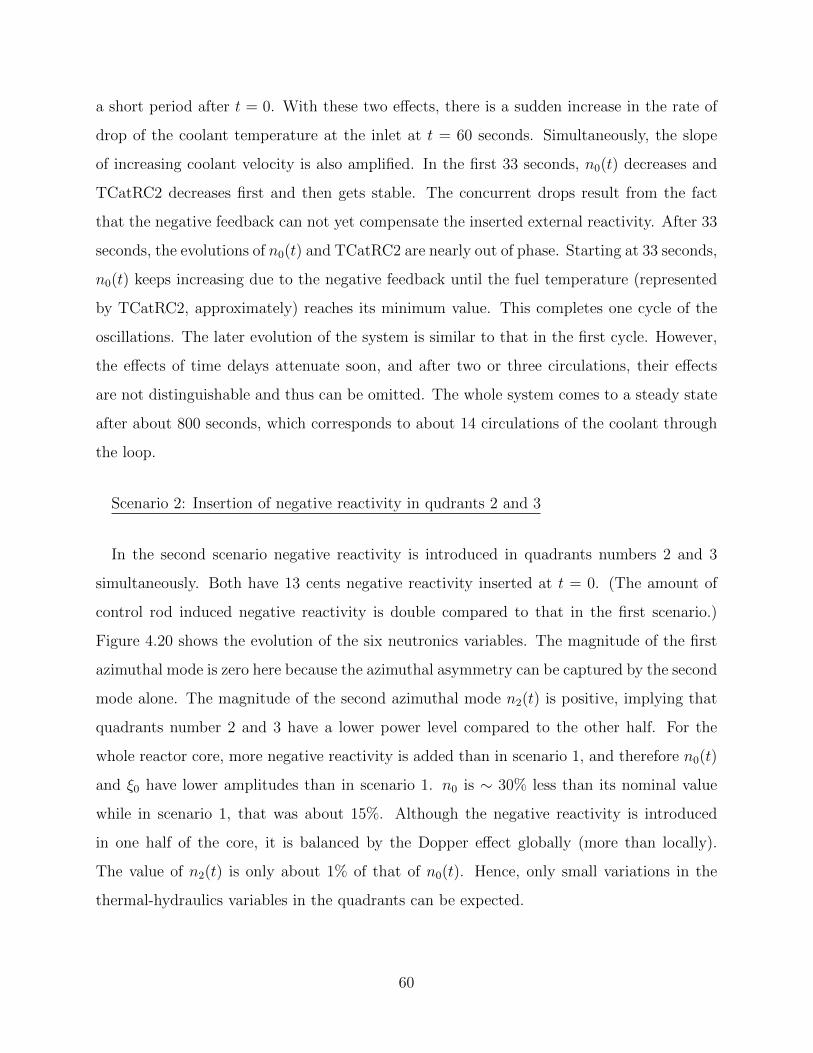
a short period after t = 0. With these two effects, there is a sudden increase in the rate of

drop of the coolant temperature at the inlet at t = 60 seconds. Simultaneously, the slope

of increasing coolant velocity is also amplified. In the first 33 seconds, n0(t) decreases and

TCatRC2 decreases first and then gets stable. The concurrent drops result from the fact

that the negative feedback can not yet compensate the inserted external reactivity. After 33

seconds, the evolutions of n0(t) and TCatRC2 are nearly out of phase. Starting at 33 seconds,

n0(t) keeps increasing due to the negative feedback until the fuel temperature (represented

by TCatRC2, approximately) reaches its minimum value. This completes one cycle of the

oscillations. The later evolution of the system is similar to that in the first cycle. However,

the effects of time delays attenuate soon, and after two or three circulations, their effects

are not distinguishable and thus can be omitted. The whole system comes to a steady state

after about 800 seconds, which corresponds to about 14 circulations of the coolant through

the loop.

Scenario 2: Insertion of negative reactivity in qudrants 2 and 3

In the second scenario negative reactivity is introduced in quadrants numbers 2 and 3

simultaneously. Both have 13 cents negative reactivity inserted at t = 0. (The amount of

control rod induced negative reactivity is double compared to that in the first scenario.)

Figure 4.20 shows the evolution of the six neutronics variables. The magnitude of the first

azimuthal mode is zero here because the azimuthal asymmetry can be captured by the second

mode alone. The magnitude of the second azimuthal mode n2(t) is positive, implying that

quadrants number 2 and 3 have a lower power level compared to the other half. For the

whole reactor core, more negative reactivity is added than in scenario 1, and therefore n0(t)

and ξ0 have lower amplitudes than in scenario 1. n0 is ∼ 30% less than its nominal value

while in scenario 1, that was about 15%. Although the negative reactivity is introduced

in one half of the core, it is balanced by the Dopper effect globally (more than locally).

The value of n2(t) is only about 1% of that of n0(t). Hence, only small variations in the

thermal-hydraulics variables in the quadrants can be expected.

60

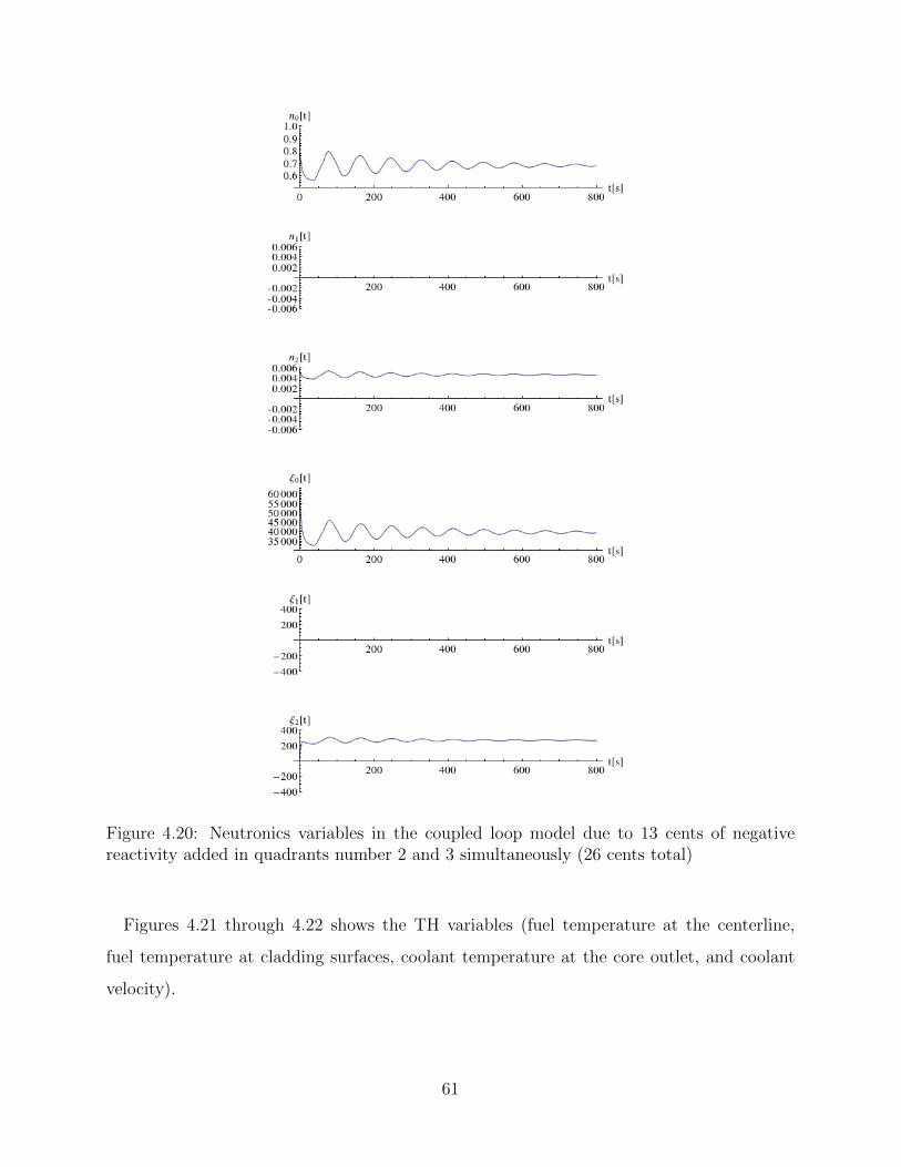
Figure 4.20: Neutronics variables in the coupled loop model due to 13 cents of negativereactivity added in quadrants number 2 and 3 simultaneously (26 cents total)

Figures 4.21 through 4.22 shows the TH variables (fuel temperature at the centerline,

fuel temperature at cladding surfaces, coolant temperature at the core outlet, and coolant

velocity).

61

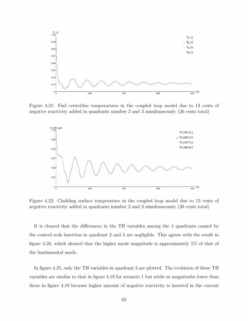
Figure 4.21: Fuel centerline temperatures in the coupled loop model due to 13 cents ofnegative reactivity added in quadrants number 2 and 3 simultaneously (26 cents total)

Figure 4.22: Cladding surface temperature in the coupled loop model due to 13 cents ofnegative reactivity added in quadrants number 2 and 3 simultaneously (26 cents total)

It is cleared that the differences in the TH variables among the 4 quadrants caused by

the control rods insertion in quadrant 2 and 3 are negligible. This agrees with the result in

figure 4.20, which showed that the higher mode magnitude is approximately 1% of that of

the fundamental mode.

In figure 4.25, only the TH variables in quadrant 2 are plotted. The evolution of these TH

variables are similar to that in figure 4.19 for scenario 1 but settle at magnitudes lower than

those in figure 4.19 because higher amount of negative reactivity is inserted in the current

62

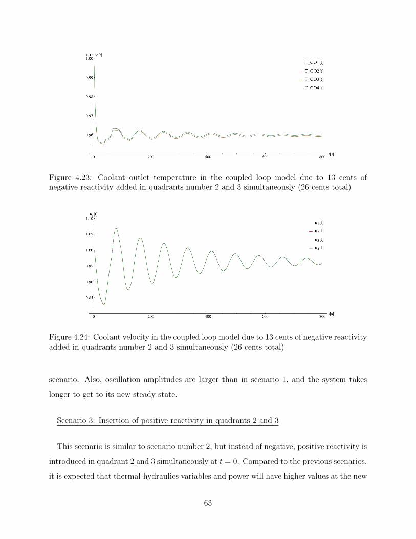
Figure 4.23: Coolant outlet temperature in the coupled loop model due to 13 cents ofnegative reactivity added in quadrants number 2 and 3 simultaneously (26 cents total)

Figure 4.24: Coolant velocity in the coupled loop model due to 13 cents of negative reactivityadded in quadrants number 2 and 3 simultaneously (26 cents total)

scenario. Also, oscillation amplitudes are larger than in scenario 1, and the system takes

longer to get to its new steady state.

Scenario 3: Insertion of positive reactivity in quadrants 2 and 3

This scenario is similar to scenario number 2, but instead of negative, positive reactivity is

introduced in quadrant 2 and 3 simultaneously at t = 0. Compared to the previous scenarios,

it is expected that thermal-hydraulics variables and power will have higher values at the new

63

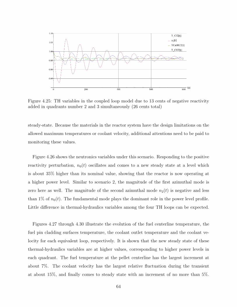
Figure 4.25: TH variables in the coupled loop model due to 13 cents of negative reactivityadded in quadrants number 2 and 3 simultaneously (26 cents total)

steady-state. Because the materials in the reactor system have the design limitations on the

allowed maximum temperatures or coolant velocity, additional attentions need to be paid to

monitoring these values.

Figure 4.26 shows the neutronics variables under this scenario. Responding to the positive

reactivity perturbation, n0(t) oscillates and comes to a new steady state at a level which

is about 35% higher than its nominal value, showing that the reactor is now operating at

a higher power level. Similar to scenario 2, the magnitude of the first azimuthal mode is

zero here as well. The magnitude of the second azimuthal mode n2(t) is negative and less

than 1% of n0(t). The fundamental mode plays the dominant role in the power level profile.

Little difference in thermal-hydraulics variables among the four TH loops can be expected.

Figures 4.27 through 4.30 illustrate the evolution of the fuel centerline temperature, the

fuel pin cladding surfaces temperature, the coolant outlet temperature and the coolant ve-

locity for each equivalent loop, respectively. It is shown that the new steady state of these

thermal-hydraulics variables are at higher values, corresponding to higher power levels in

each quadrant. The fuel temperature at the pellet centerline has the largest increment at

about 7%. The coolant velocity has the largest relative fluctuation during the transient

at about 15%, and finally comes to steady state with an increment of no more than 5%.

64

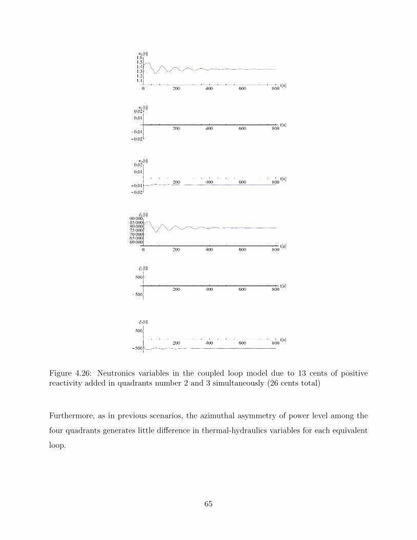
Figure 4.26: Neutronics variables in the coupled loop model due to 13 cents of positivereactivity added in quadrants number 2 and 3 simultaneously (26 cents total)

Furthermore, as in previous scenarios, the azimuthal asymmetry of power level among the

four quadrants generates little difference in thermal-hydraulics variables for each equivalent

loop.

65

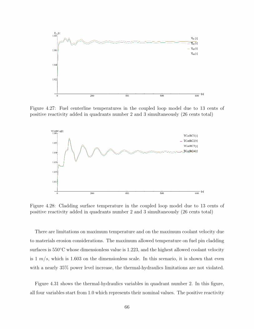
Figure 4.27: Fuel centerline temperatures in the coupled loop model due to 13 cents ofpositive reactivity added in quadrants number 2 and 3 simultaneously (26 cents total)

Figure 4.28: Cladding surface temperature in the coupled loop model due to 13 cents ofpositive reactivity added in quadrants number 2 and 3 simultaneously (26 cents total)

There are limitations on maximum temperature and on the maximum coolant velocity due

to materials erosion considerations. The maximum allowed temperature on fuel pin cladding

surfaces is 550◦C whose dimensionless value is 1.223, and the highest allowed coolant velocity

is 1 m/s, which is 1.603 on the dimensionless scale. In this scenario, it is shown that even

with a nearly 35% power level increase, the thermal-hydraulics limitations are not violated.

Figure 4.31 shows the thermal-hydraulics variables in quadrant number 2. In this figure,

all four variables start from 1.0 which represents their nominal values. The positive reactivity

66

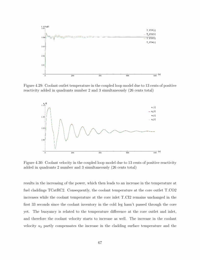
Figure 4.29: Coolant outlet temperature in the coupled loop model due to 13 cents of positivereactivity added in quadrants number 2 and 3 simultaneously (26 cents total)

Figure 4.30: Coolant velocity in the coupled loop model due to 13 cents of positive reactivityadded in quadrants 2 number and 3 simultaneously (26 cents total)

results in the increasing of the power, which then leads to an increase in the temperature at

fuel claddings TCatRC2. Consequently, the coolant temperature at the core outlet T CO2

increases while the coolant temperature at the core inlet T CI2 remains unchanged in the

first 33 seconds since the coolant inventory in the cold leg hasn’t passed through the core

yet. The buoyancy is related to the temperature difference at the core outlet and inlet,

and therefore the coolant velocity starts to increase as well. The increase in the coolant

velocity u2 partly compensates the increase in the cladding surface temperature and the

67

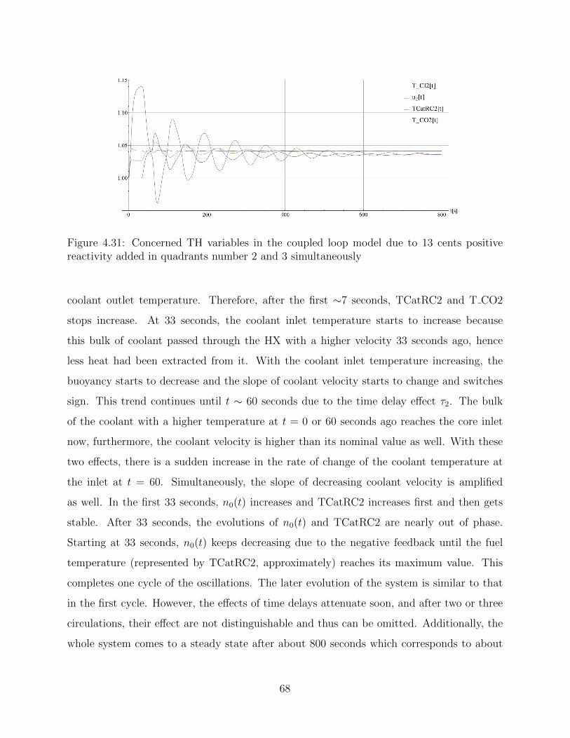
Figure 4.31: Concerned TH variables in the coupled loop model due to 13 cents positivereactivity added in quadrants number 2 and 3 simultaneously

coolant outlet temperature. Therefore, after the first ∼7 seconds, TCatRC2 and T CO2

stops increase. At 33 seconds, the coolant inlet temperature starts to increase because

this bulk of coolant passed through the HX with a higher velocity 33 seconds ago, hence

less heat had been extracted from it. With the coolant inlet temperature increasing, the

buoyancy starts to decrease and the slope of coolant velocity starts to change and switches

sign. This trend continues until t ∼ 60 seconds due to the time delay effect τ2. The bulk

of the coolant with a higher temperature at t = 0 or 60 seconds ago reaches the core inlet

now, furthermore, the coolant velocity is higher than its nominal value as well. With these

two effects, there is a sudden increase in the rate of change of the coolant temperature at

the inlet at t = 60. Simultaneously, the slope of decreasing coolant velocity is amplified

as well. In the first 33 seconds, n0(t) increases and TCatRC2 increases first and then gets

stable. After 33 seconds, the evolutions of n0(t) and TCatRC2 are nearly out of phase.

Starting at 33 seconds, n0(t) keeps decreasing due to the negative feedback until the fuel

temperature (represented by TCatRC2, approximately) reaches its maximum value. This

completes one cycle of the oscillations. The later evolution of the system is similar to that

in the first cycle. However, the effects of time delays attenuate soon, and after two or three

circulations, their effect are not distinguishable and thus can be omitted. Additionally, the

whole system comes to a steady state after about 800 seconds which corresponds to about

68

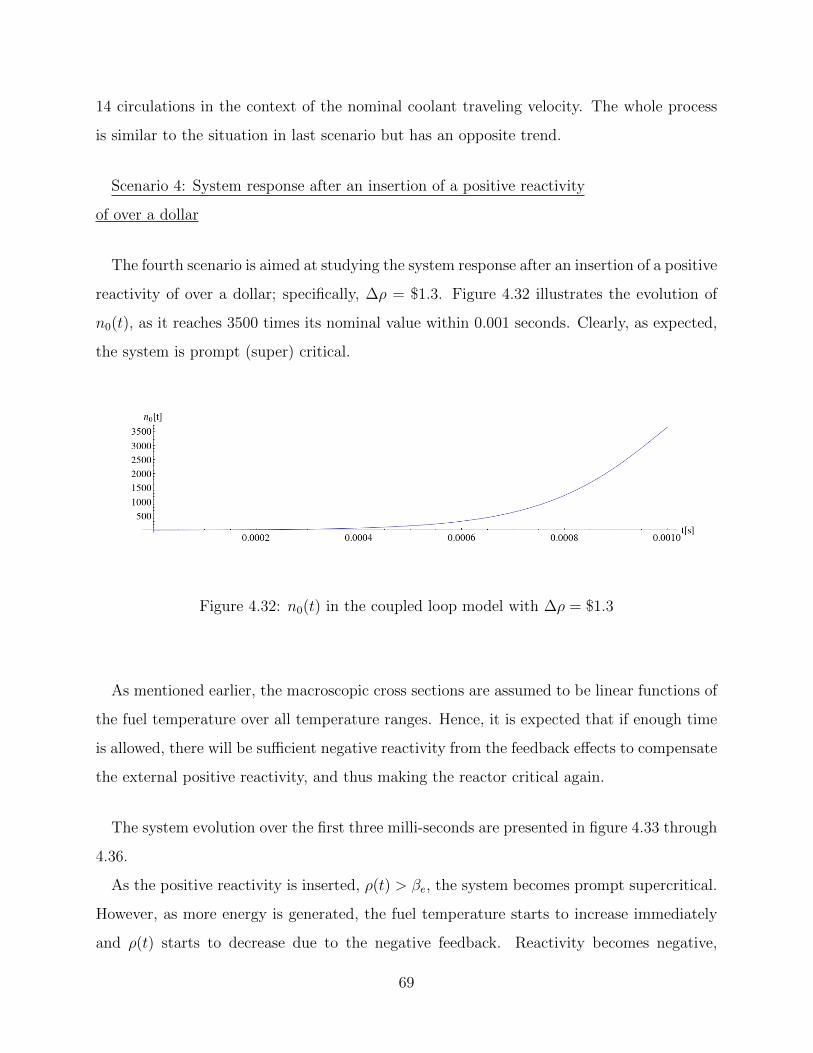
14 circulations in the context of the nominal coolant traveling velocity. The whole process

is similar to the situation in last scenario but has an opposite trend.

Scenario 4: System response after an insertion of a positive reactivity

of over a dollar

The fourth scenario is aimed at studying the system response after an insertion of a positive

reactivity of over a dollar; specifically, ∆ρ = $1.3. Figure 4.32 illustrates the evolution of

n0(t), as it reaches 3500 times its nominal value within 0.001 seconds. Clearly, as expected,

the system is prompt (super) critical.

Figure 4.32: n0(t) in the coupled loop model with ∆ρ = $1.3

As mentioned earlier, the macroscopic cross sections are assumed to be linear functions of

the fuel temperature over all temperature ranges. Hence, it is expected that if enough time

is allowed, there will be sufficient negative reactivity from the feedback effects to compensate

the external positive reactivity, and thus making the reactor critical again.

The system evolution over the first three milli-seconds are presented in figure 4.33 through

4.36.

As the positive reactivity is inserted, ρ(t) > βe, the system becomes prompt supercritical.

However, as more energy is generated, the fuel temperature starts to increase immediately

and ρ(t) starts to decrease due to the negative feedback. Reactivity becomes negative,

69

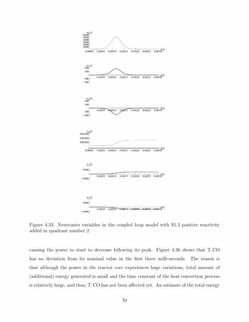
Figure 4.33: Neutronics variables in the coupled loop model with $1.3 positive reactivityadded in quadrant number 2

causing the power to start to decrease following its peak. Figure 4.36 shows that T CO

has no deviation from its nominal value in the first three milli-seconds. The reason is

that although the power in the reactor core experiences huge variations, total amount of

(additional) energy generated is small and the time constant of the heat convection process

is relatively large, and thus, T CO has not been affected yet. An estimate of the total energy

70

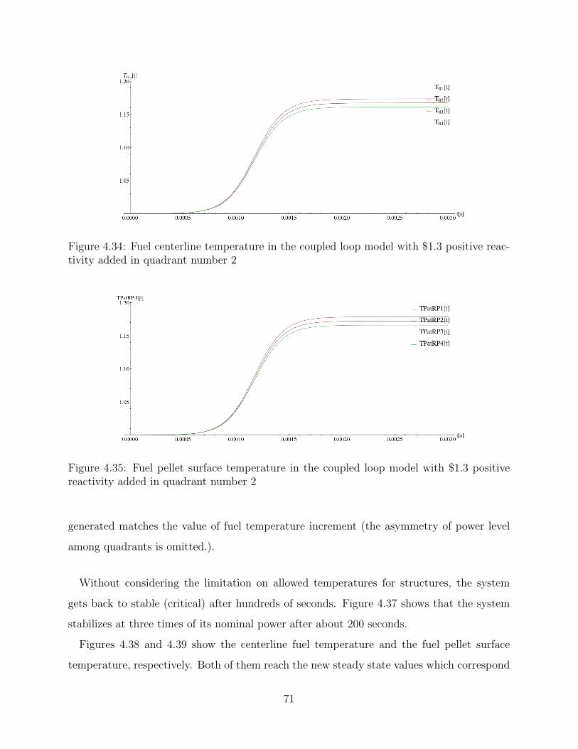
Figure 4.34: Fuel centerline temperature in the coupled loop model with $1.3 positive reac-tivity added in quadrant number 2

Figure 4.35: Fuel pellet surface temperature in the coupled loop model with $1.3 positivereactivity added in quadrant number 2

generated matches the value of fuel temperature increment (the asymmetry of power level

among quadrants is omitted.).

Without considering the limitation on allowed temperatures for structures, the system

gets back to stable (critical) after hundreds of seconds. Figure 4.37 shows that the system

stabilizes at three times of its nominal power after about 200 seconds.

Figures 4.38 and 4.39 show the centerline fuel temperature and the fuel pellet surface

temperature, respectively. Both of them reach the new steady state values which correspond

71

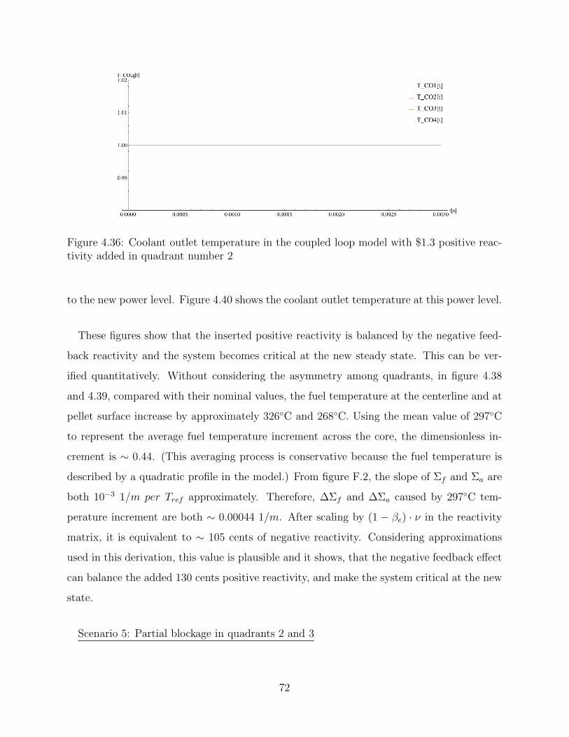
Figure 4.36: Coolant outlet temperature in the coupled loop model with $1.3 positive reac-tivity added in quadrant number 2

to the new power level. Figure 4.40 shows the coolant outlet temperature at this power level.

These figures show that the inserted positive reactivity is balanced by the negative feed-

back reactivity and the system becomes critical at the new steady state. This can be ver-

ified quantitatively. Without considering the asymmetry among quadrants, in figure 4.38

and 4.39, compared with their nominal values, the fuel temperature at the centerline and at

pellet surface increase by approximately 326◦C and 268◦C. Using the mean value of 297◦C

to represent the average fuel temperature increment across the core, the dimensionless in-

crement is ∼ 0.44. (This averaging process is conservative because the fuel temperature is

described by a quadratic profile in the model.) From figure F.2, the slope of Σf and Σa are

both 10−3 1/m per Tref approximately. Therefore, ∆Σf and ∆Σa caused by 297◦C tem-

perature increment are both ∼ 0.00044 1/m. After scaling by (1 − βe) · ν in the reactivity

matrix, it is equivalent to ∼ 105 cents of negative reactivity. Considering approximations

used in this derivation, this value is plausible and it shows, that the negative feedback effect

can balance the added 130 cents positive reactivity, and make the system critical at the new

state.

Scenario 5: Partial blockage in quadrants 2 and 3

72

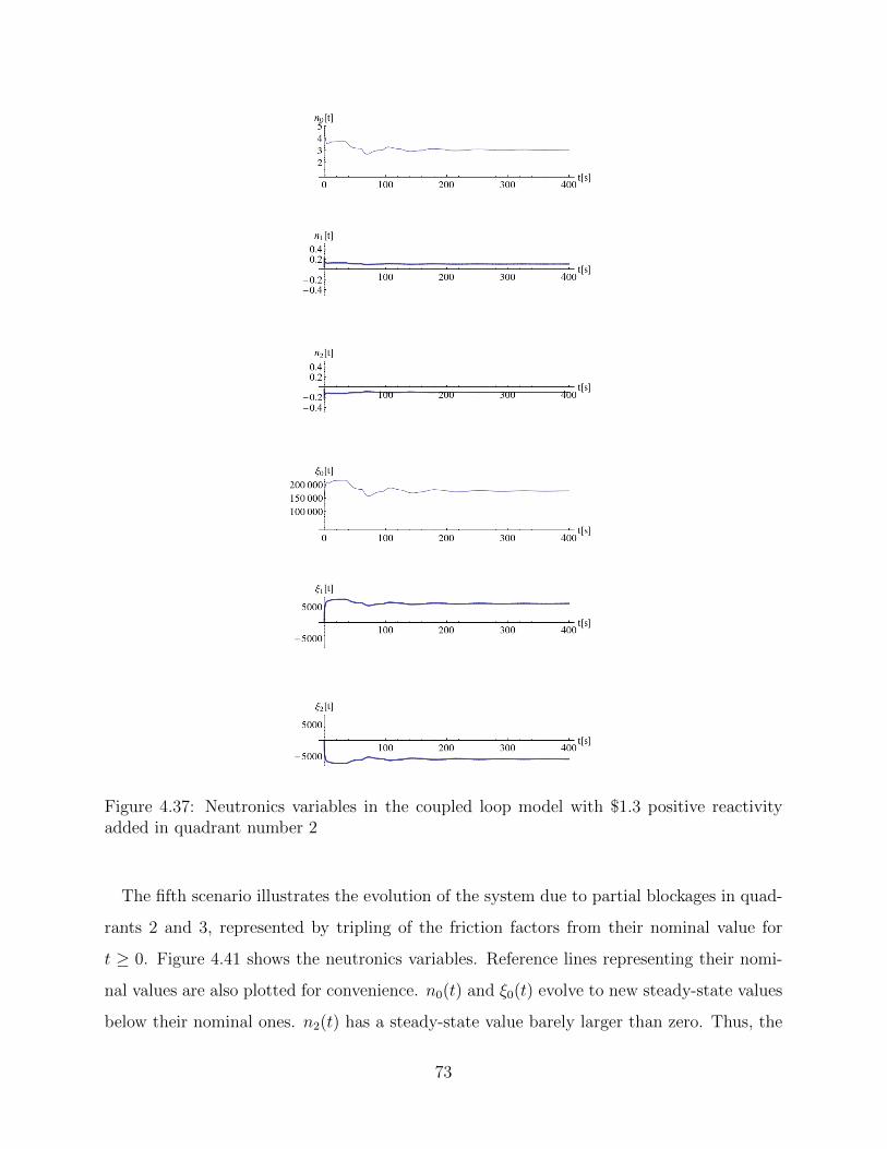
Figure 4.37: Neutronics variables in the coupled loop model with $1.3 positive reactivityadded in quadrant number 2

The fifth scenario illustrates the evolution of the system due to partial blockages in quad-

rants 2 and 3, represented by tripling of the friction factors from their nominal value for

t ≥ 0. Figure 4.41 shows the neutronics variables. Reference lines representing their nomi-

nal values are also plotted for convenience. n0(t) and ξ0(t) evolve to new steady-state values

below their nominal ones. n2(t) has a steady-state value barely larger than zero. Thus, the

73

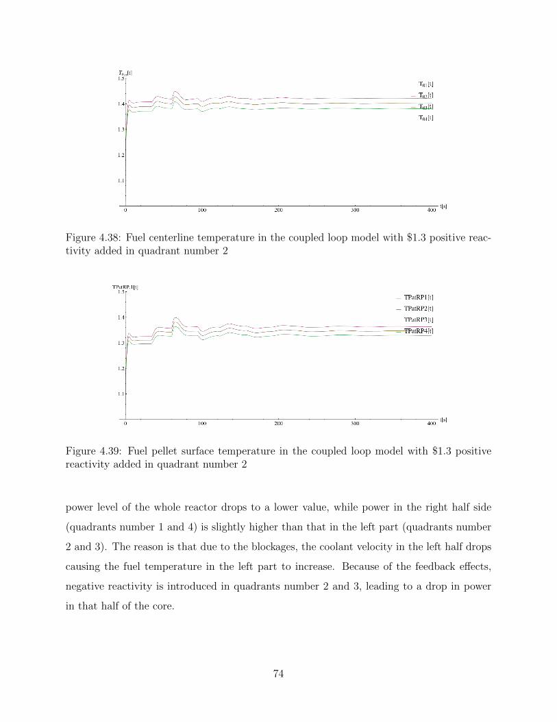
Figure 4.38: Fuel centerline temperature in the coupled loop model with $1.3 positive reac-tivity added in quadrant number 2

Figure 4.39: Fuel pellet surface temperature in the coupled loop model with $1.3 positivereactivity added in quadrant number 2

power level of the whole reactor drops to a lower value, while power in the right half side

(quadrants number 1 and 4) is slightly higher than that in the left part (quadrants number

2 and 3). The reason is that due to the blockages, the coolant velocity in the left half drops

causing the fuel temperature in the left part to increase. Because of the feedback effects,

negative reactivity is introduced in quadrants number 2 and 3, leading to a drop in power

in that half of the core.

74

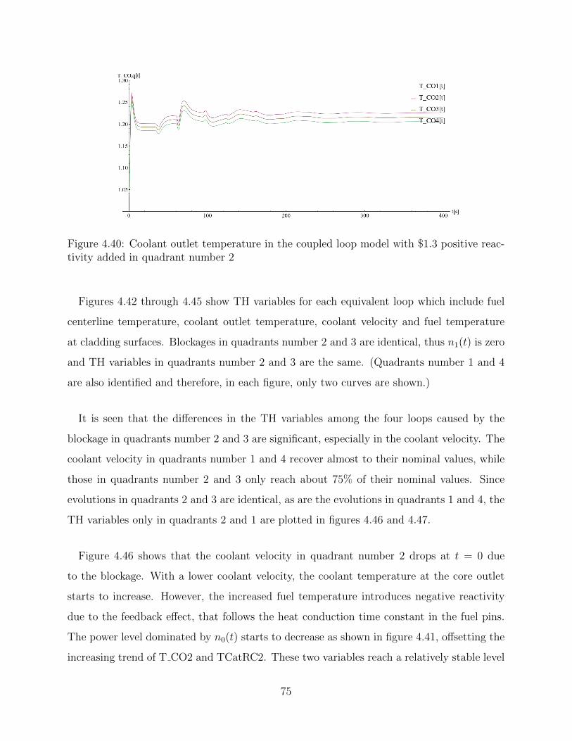
Figure 4.40: Coolant outlet temperature in the coupled loop model with $1.3 positive reac-tivity added in quadrant number 2

Figures 4.42 through 4.45 show TH variables for each equivalent loop which include fuel

centerline temperature, coolant outlet temperature, coolant velocity and fuel temperature

at cladding surfaces. Blockages in quadrants number 2 and 3 are identical, thus n1(t) is zero

and TH variables in quadrants number 2 and 3 are the same. (Quadrants number 1 and 4

are also identified and therefore, in each figure, only two curves are shown.)

It is seen that the differences in the TH variables among the four loops caused by the

blockage in quadrants number 2 and 3 are significant, especially in the coolant velocity. The

coolant velocity in quadrants number 1 and 4 recover almost to their nominal values, while

those in quadrants number 2 and 3 only reach about 75% of their nominal values. Since

evolutions in quadrants 2 and 3 are identical, as are the evolutions in quadrants 1 and 4, the

TH variables only in quadrants 2 and 1 are plotted in figures 4.46 and 4.47.

Figure 4.46 shows that the coolant velocity in quadrant number 2 drops at t = 0 due

to the blockage. With a lower coolant velocity, the coolant temperature at the core outlet

starts to increase. However, the increased fuel temperature introduces negative reactivity

due to the feedback effect, that follows the heat conduction time constant in the fuel pins.

The power level dominated by n0(t) starts to decrease as shown in figure 4.41, offsetting the

increasing trend of T CO2 and TCatRC2. These two variables reach a relatively stable level

75

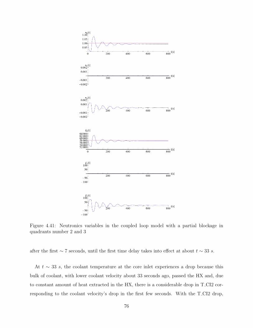
Figure 4.41: Neutronics variables in the coupled loop model with a partial blockage inquadrants number 2 and 3

after the first ∼ 7 seconds, until the first time delay takes into effect at about t ∼ 33 s.

At t ∼ 33 s, the coolant temperature at the core inlet experiences a drop because this

bulk of coolant, with lower coolant velocity about 33 seconds ago, passed the HX and, due

to constant amount of heat extracted in the HX, there is a considerable drop in T CI2 cor-

responding to the coolant velocity’s drop in the first few seconds. With the T CI2 drop,

76

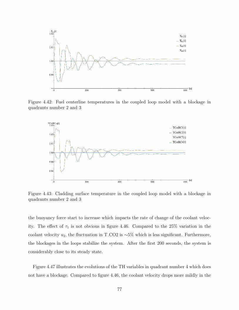
Figure 4.42: Fuel centerline temperatures in the coupled loop model with a blockage inquadrants number 2 and 3

Figure 4.43: Cladding surface temperature in the coupled loop model with a blockage inquadrants number 2 and 3

the buoyancy force start to increase which impacts the rate of change of the coolant veloc-

ity. The effect of τ1 is not obvious in figure 4.46. Compared to the 25% variation in the

coolant velocity u2, the fluctuation in T CO2 is ∼5% which is less significant. Furthermore,

the blockages in the loops stabilize the system. After the first 200 seconds, the system is

considerably close to its steady state.

Figure 4.47 illustrates the evolutions of the TH variables in quadrant number 4 which does

not have a blockage. Compared to figure 4.46, the coolant velocity drops more mildly in the

77

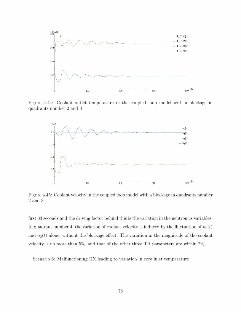
Figure 4.44: Coolant outlet temperature in the coupled loop model with a blockage inquadrants number 2 and 3

Figure 4.45: Coolant velocity in the coupled loop model with a blockage in quadrants number2 and 3

first 33 seconds and the driving factor behind this is the variation in the neutronics variables.

In quadrant number 4, the variation of coolant velocity is induced by the fluctuation of n0(t)

and n2(t) alone, without the blockage effect. The variation in the magnitude of the coolant

velocity is no more than 5%, and that of the other three TH parameters are within 2%.

Scenario 6: Malfunctioning HX leading to variation in core inlet temperature

78

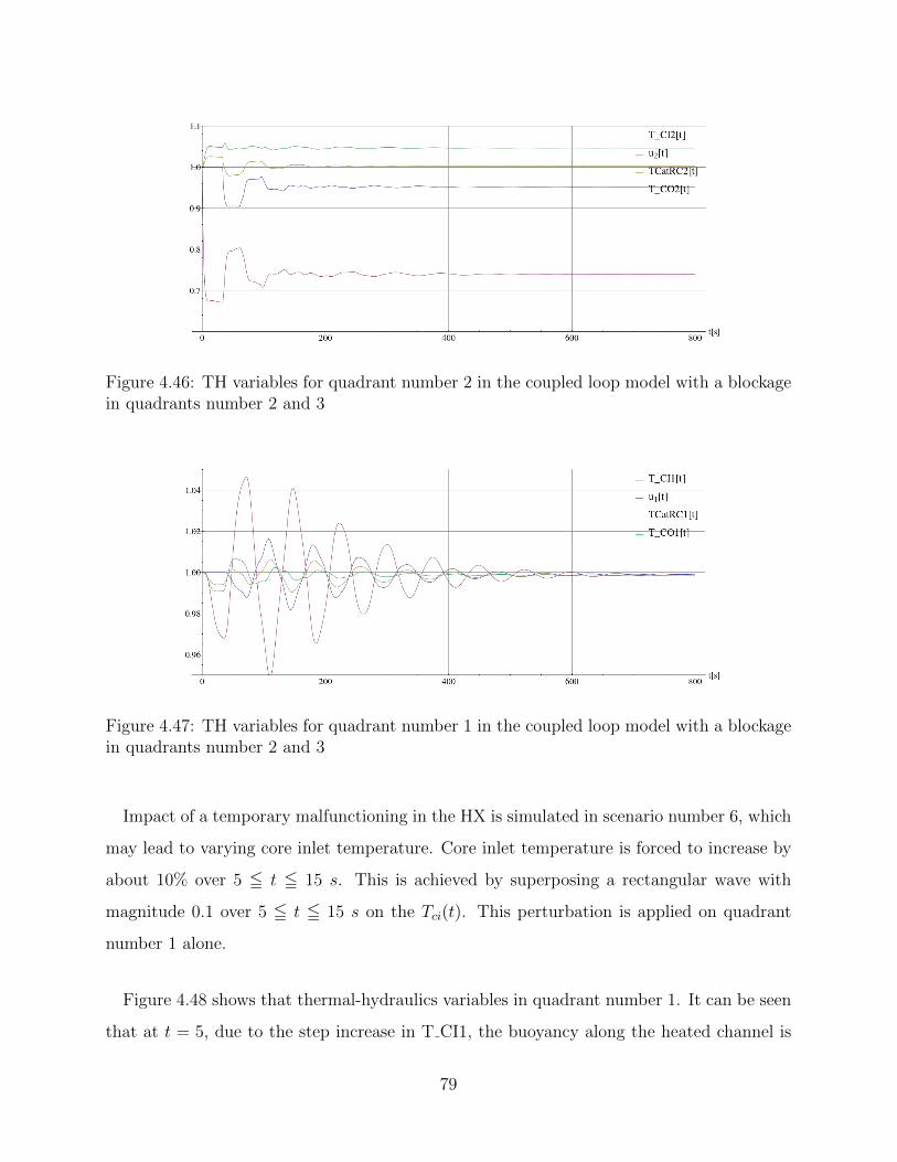
Figure 4.46: TH variables for quadrant number 2 in the coupled loop model with a blockagein quadrants number 2 and 3

Figure 4.47: TH variables for quadrant number 1 in the coupled loop model with a blockagein quadrants number 2 and 3

Impact of a temporary malfunctioning in the HX is simulated in scenario number 6, which

may lead to varying core inlet temperature. Core inlet temperature is forced to increase by

about 10% over 5 5 t 5 15 s. This is achieved by superposing a rectangular wave with

magnitude 0.1 over 5 5 t 5 15 s on the Tci(t). This perturbation is applied on quadrant

number 1 alone.

Figure 4.48 shows that thermal-hydraulics variables in quadrant number 1. It can be seen

that at t = 5, due to the step increase in T CI1, the buoyancy along the heated channel is

79

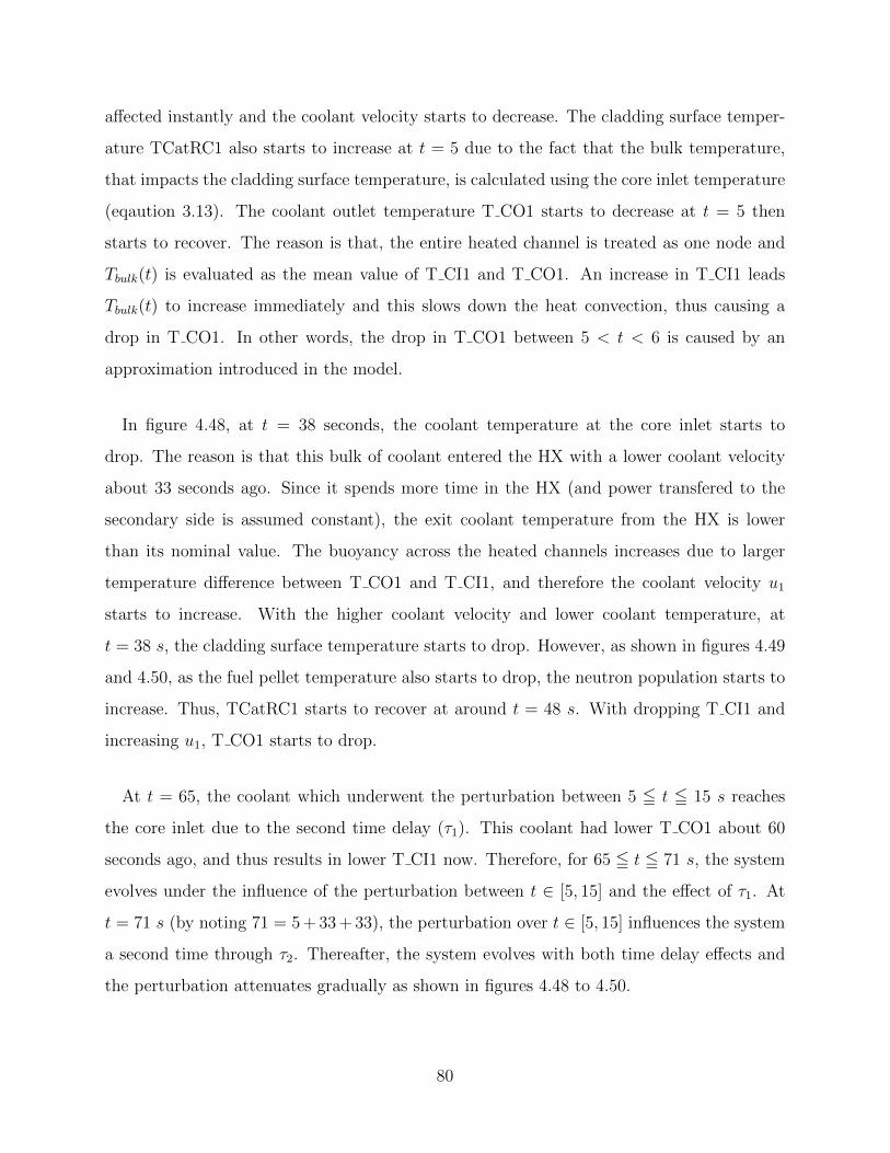
affected instantly and the coolant velocity starts to decrease. The cladding surface temper-

ature TCatRC1 also starts to increase at t = 5 due to the fact that the bulk temperature,

that impacts the cladding surface temperature, is calculated using the core inlet temperature

(eqaution 3.13). The coolant outlet temperature T CO1 starts to decrease at t = 5 then

starts to recover. The reason is that, the entire heated channel is treated as one node and

Tbulk(t) is evaluated as the mean value of T CI1 and T CO1. An increase in T CI1 leads

Tbulk(t) to increase immediately and this slows down the heat convection, thus causing a

drop in T CO1. In other words, the drop in T CO1 between 5 < t < 6 is caused by an

approximation introduced in the model.

In figure 4.48, at t = 38 seconds, the coolant temperature at the core inlet starts to

drop. The reason is that this bulk of coolant entered the HX with a lower coolant velocity

about 33 seconds ago. Since it spends more time in the HX (and power transfered to the

secondary side is assumed constant), the exit coolant temperature from the HX is lower

than its nominal value. The buoyancy across the heated channels increases due to larger

temperature difference between T CO1 and T CI1, and therefore the coolant velocity u1

starts to increase. With the higher coolant velocity and lower coolant temperature, at

t = 38 s, the cladding surface temperature starts to drop. However, as shown in figures 4.49

and 4.50, as the fuel pellet temperature also starts to drop, the neutron population starts to

increase. Thus, TCatRC1 starts to recover at around t = 48 s. With dropping T CI1 and

increasing u1, T CO1 starts to drop.

At t = 65, the coolant which underwent the perturbation between 5 5 t 5 15 s reaches

the core inlet due to the second time delay (τ1). This coolant had lower T CO1 about 60

seconds ago, and thus results in lower T CI1 now. Therefore, for 65 5 t 5 71 s, the system

evolves under the influence of the perturbation between t ∈ [5, 15] and the effect of τ1. At

t = 71 s (by noting 71 = 5 + 33 + 33), the perturbation over t ∈ [5, 15] influences the system

a second time through τ2. Thereafter, the system evolves with both time delay effects and

the perturbation attenuates gradually as shown in figures 4.48 to 4.50.

80

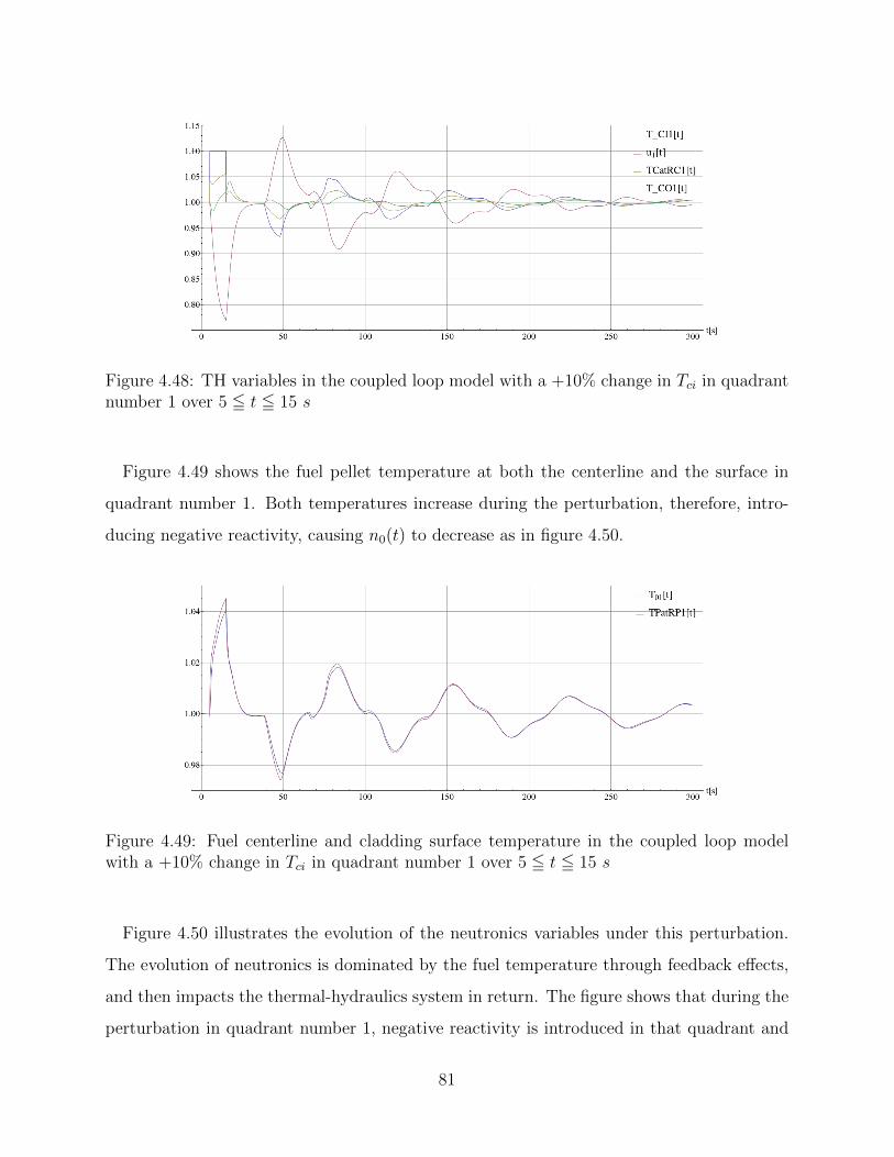
Figure 4.48: TH variables in the coupled loop model with a +10% change in Tci in quadrantnumber 1 over 5 5 t 5 15 s

Figure 4.49 shows the fuel pellet temperature at both the centerline and the surface in

quadrant number 1. Both temperatures increase during the perturbation, therefore, intro-

ducing negative reactivity, causing n0(t) to decrease as in figure 4.50.

Figure 4.49: Fuel centerline and cladding surface temperature in the coupled loop modelwith a +10% change in Tci in quadrant number 1 over 5 5 t 5 15 s

Figure 4.50 illustrates the evolution of the neutronics variables under this perturbation.

The evolution of neutronics is dominated by the fuel temperature through feedback effects,

and then impacts the thermal-hydraulics system in return. The figure shows that during the

perturbation in quadrant number 1, negative reactivity is introduced in that quadrant and

81

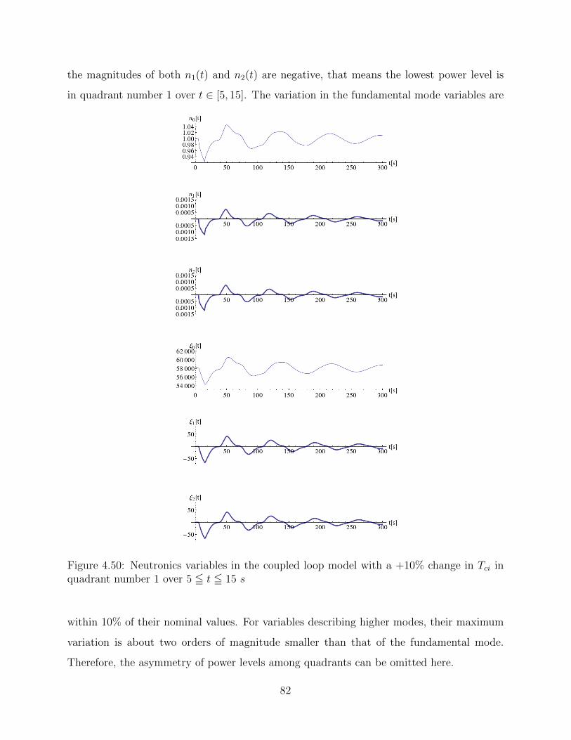
the magnitudes of both n1(t) and n2(t) are negative, that means the lowest power level is

in quadrant number 1 over t ∈ [5, 15]. The variation in the fundamental mode variables are

Figure 4.50: Neutronics variables in the coupled loop model with a +10% change in Tci inquadrant number 1 over 5 5 t 5 15 s

within 10% of their nominal values. For variables describing higher modes, their maximum

variation is about two orders of magnitude smaller than that of the fundamental mode.

Therefore, the asymmetry of power levels among quadrants can be omitted here.

82

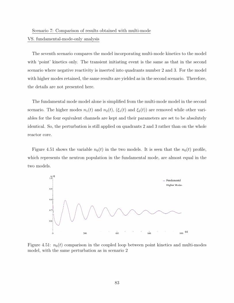
Scenario 7: Comparison of results obtained with multi-mode

VS. fundamental-mode-only analysis

The seventh scenario compares the model incorporating multi-mode kinetics to the model

with ‘point’ kinetics only. The transient initiating event is the same as that in the second

scenario where negative reactivity is inserted into quadrants number 2 and 3. For the model

with higher modes retained, the same results are yielded as in the second scenario. Therefore,

the details are not presented here.

The fundamental mode model alone is simplified from the multi-mode model in the second

scenario. The higher modes n1(t) and n2(t), (ξ1(t) and ξ2(t)) are removed while other vari-

ables for the four equivalent channels are kept and their parameters are set to be absolutely

identical. So, the perturbation is still applied on quadrants 2 and 3 rather than on the whole

reactor core.

Figure 4.51 shows the variable n0(t) in the two models. It is seen that the n0(t) profile,

which represents the neutron population in the fundamental mode, are almost equal in the

two models.

Figure 4.51: n0(t) comparison in the coupled loop between point kinetics and multi-modesmodel, with the same perturbation as in scenario 2

83

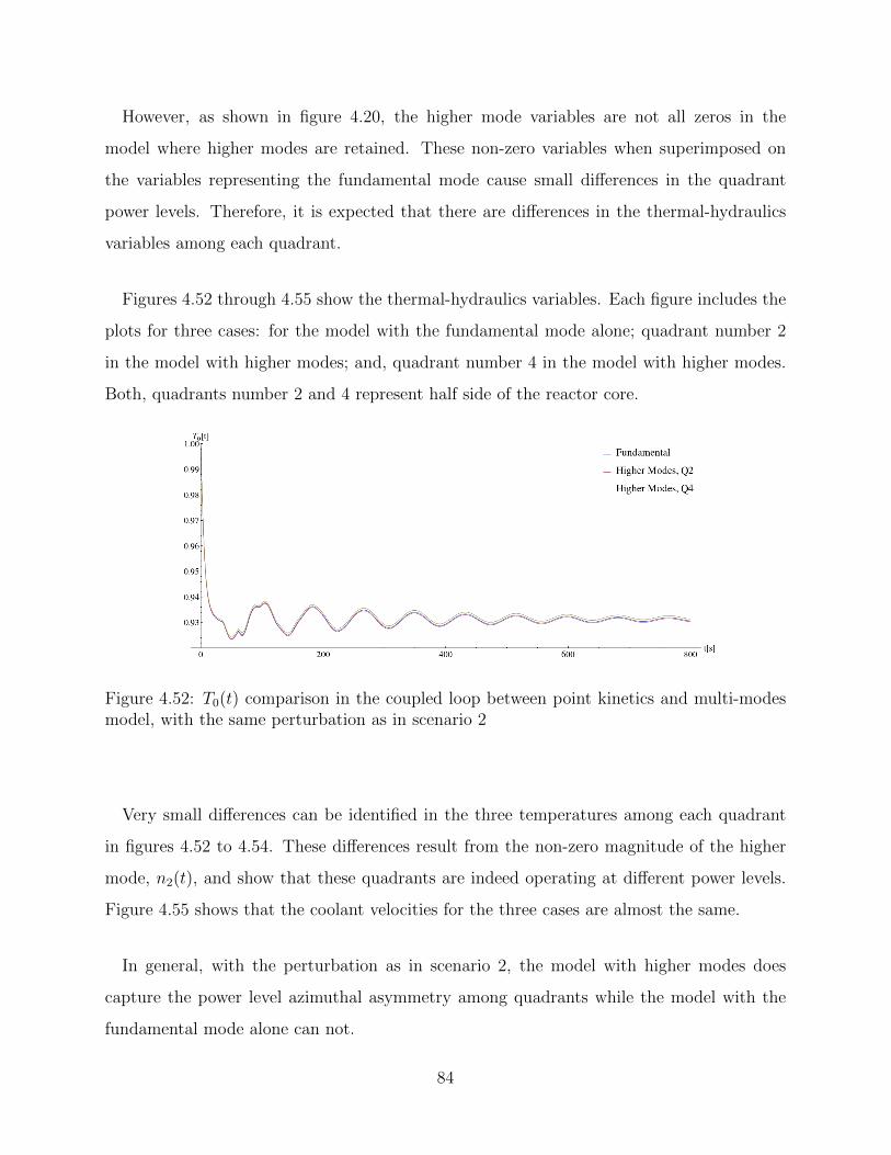
However, as shown in figure 4.20, the higher mode variables are not all zeros in the

model where higher modes are retained. These non-zero variables when superimposed on

the variables representing the fundamental mode cause small differences in the quadrant

power levels. Therefore, it is expected that there are differences in the thermal-hydraulics

variables among each quadrant.

Figures 4.52 through 4.55 show the thermal-hydraulics variables. Each figure includes the

plots for three cases: for the model with the fundamental mode alone; quadrant number 2

in the model with higher modes; and, quadrant number 4 in the model with higher modes.

Both, quadrants number 2 and 4 represent half side of the reactor core.

Figure 4.52: T0(t) comparison in the coupled loop between point kinetics and multi-modesmodel, with the same perturbation as in scenario 2

Very small differences can be identified in the three temperatures among each quadrant

in figures 4.52 to 4.54. These differences result from the non-zero magnitude of the higher

mode, n2(t), and show that these quadrants are indeed operating at different power levels.

Figure 4.55 shows that the coolant velocities for the three cases are almost the same.

In general, with the perturbation as in scenario 2, the model with higher modes does

capture the power level azimuthal asymmetry among quadrants while the model with the

fundamental mode alone can not.

84

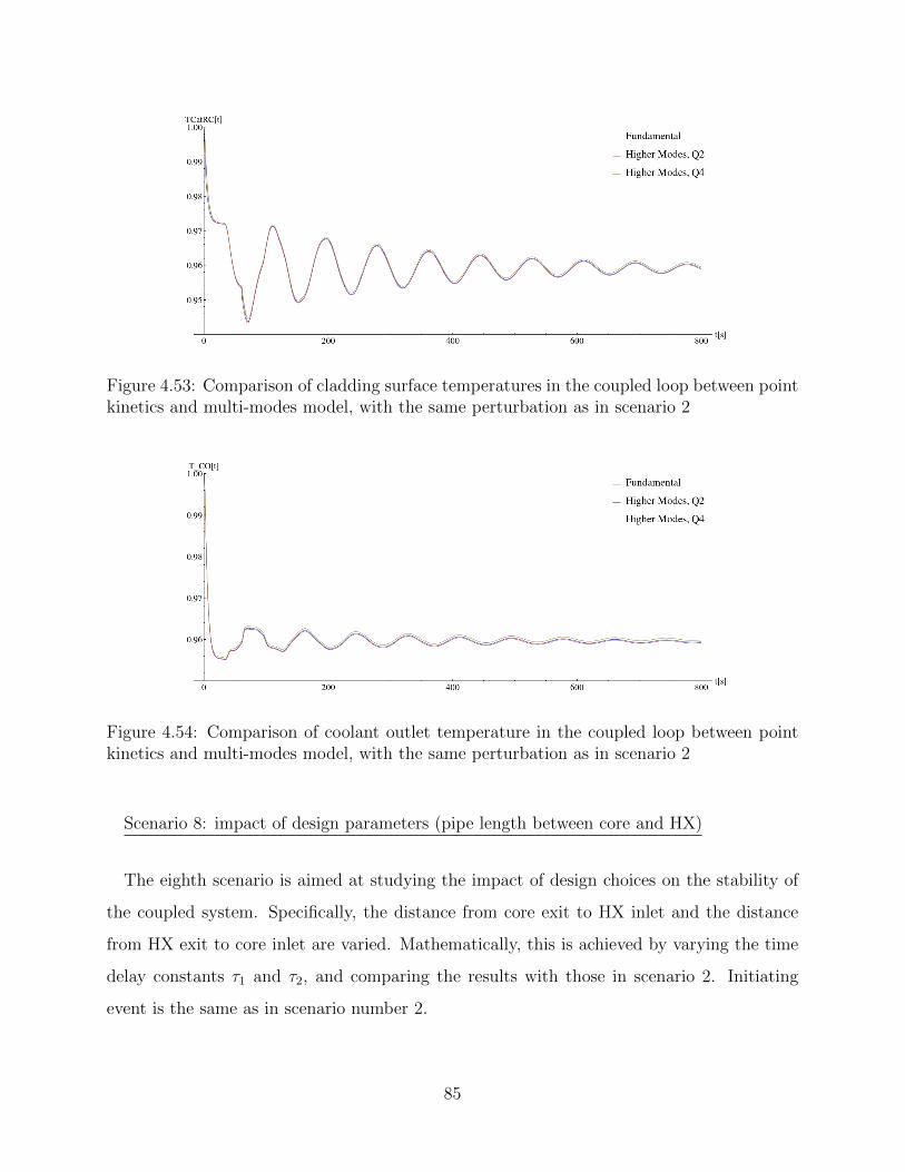
Figure 4.53: Comparison of cladding surface temperatures in the coupled loop between pointkinetics and multi-modes model, with the same perturbation as in scenario 2

Figure 4.54: Comparison of coolant outlet temperature in the coupled loop between pointkinetics and multi-modes model, with the same perturbation as in scenario 2

Scenario 8: impact of design parameters (pipe length between core and HX)

The eighth scenario is aimed at studying the impact of design choices on the stability of

the coupled system. Specifically, the distance from core exit to HX inlet and the distance

from HX exit to core inlet are varied. Mathematically, this is achieved by varying the time

delay constants τ1 and τ2, and comparing the results with those in scenario 2. Initiating

event is the same as in scenario number 2.

85

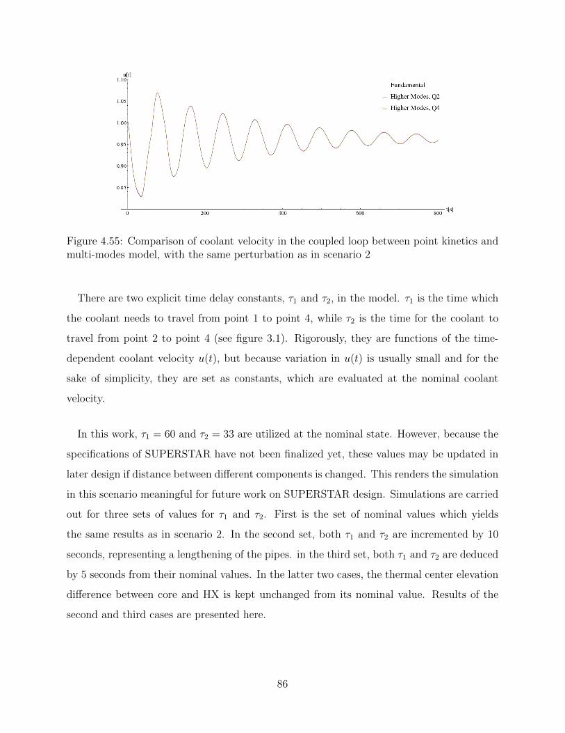
Figure 4.55: Comparison of coolant velocity in the coupled loop between point kinetics andmulti-modes model, with the same perturbation as in scenario 2

There are two explicit time delay constants, τ1 and τ2, in the model. τ1 is the time which

the coolant needs to travel from point 1 to point 4, while τ2 is the time for the coolant to

travel from point 2 to point 4 (see figure 3.1). Rigorously, they are functions of the time-

dependent coolant velocity u(t), but because variation in u(t) is usually small and for the

sake of simplicity, they are set as constants, which are evaluated at the nominal coolant

velocity.

In this work, τ1 = 60 and τ2 = 33 are utilized at the nominal state. However, because the

specifications of SUPERSTAR have not been finalized yet, these values may be updated in

later design if distance between different components is changed. This renders the simulation

in this scenario meaningful for future work on SUPERSTAR design. Simulations are carried

out for three sets of values for τ1 and τ2. First is the set of nominal values which yields

the same results as in scenario 2. In the second set, both τ1 and τ2 are incremented by 10

seconds, representing a lengthening of the pipes. in the third set, both τ1 and τ2 are deduced

by 5 seconds from their nominal values. In the latter two cases, the thermal center elevation

difference between core and HX is kept unchanged from its nominal value. Results of the

second and third cases are presented here.

86

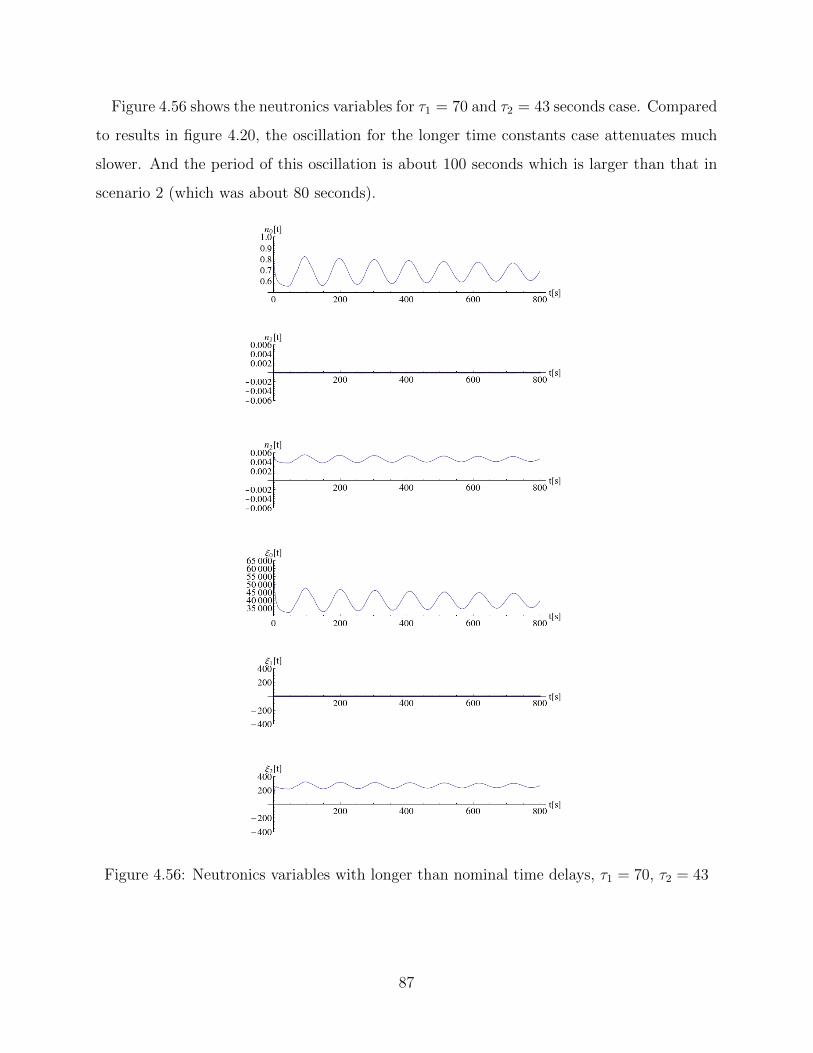
Figure 4.56 shows the neutronics variables for τ1 = 70 and τ2 = 43 seconds case. Compared

to results in figure 4.20, the oscillation for the longer time constants case attenuates much

slower. And the period of this oscillation is about 100 seconds which is larger than that in

scenario 2 (which was about 80 seconds).

Figure 4.56: Neutronics variables with longer than nominal time delays, τ1 = 70, τ2 = 43

87

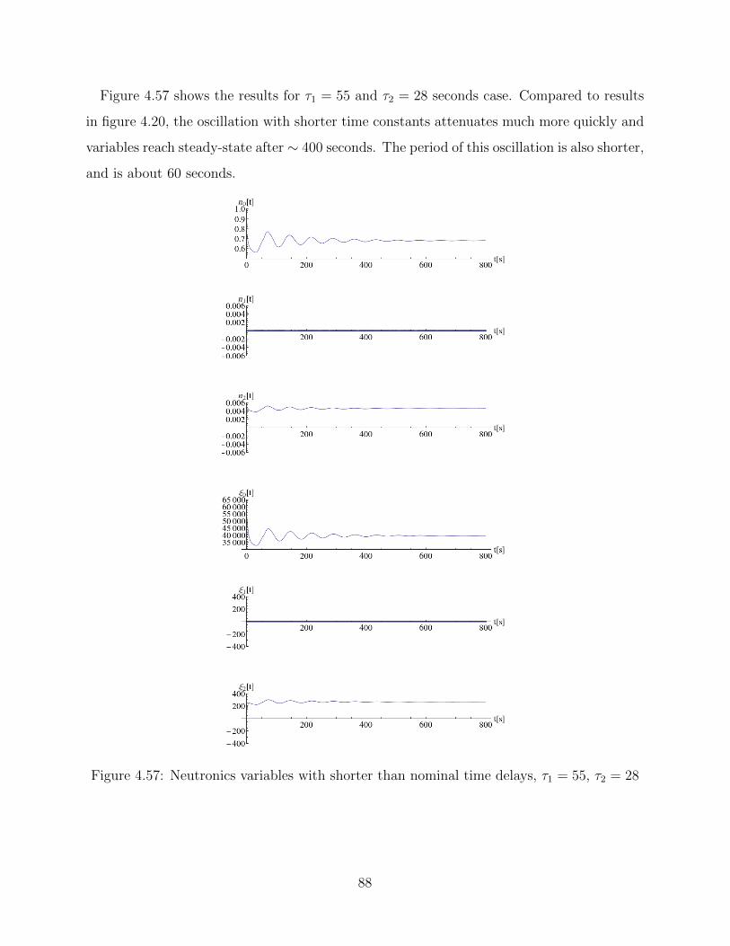
Figure 4.57 shows the results for τ1 = 55 and τ2 = 28 seconds case. Compared to results

in figure 4.20, the oscillation with shorter time constants attenuates much more quickly and

variables reach steady-state after ∼ 400 seconds. The period of this oscillation is also shorter,

and is about 60 seconds.

Figure 4.57: Neutronics variables with shorter than nominal time delays, τ1 = 55, τ2 = 28

88

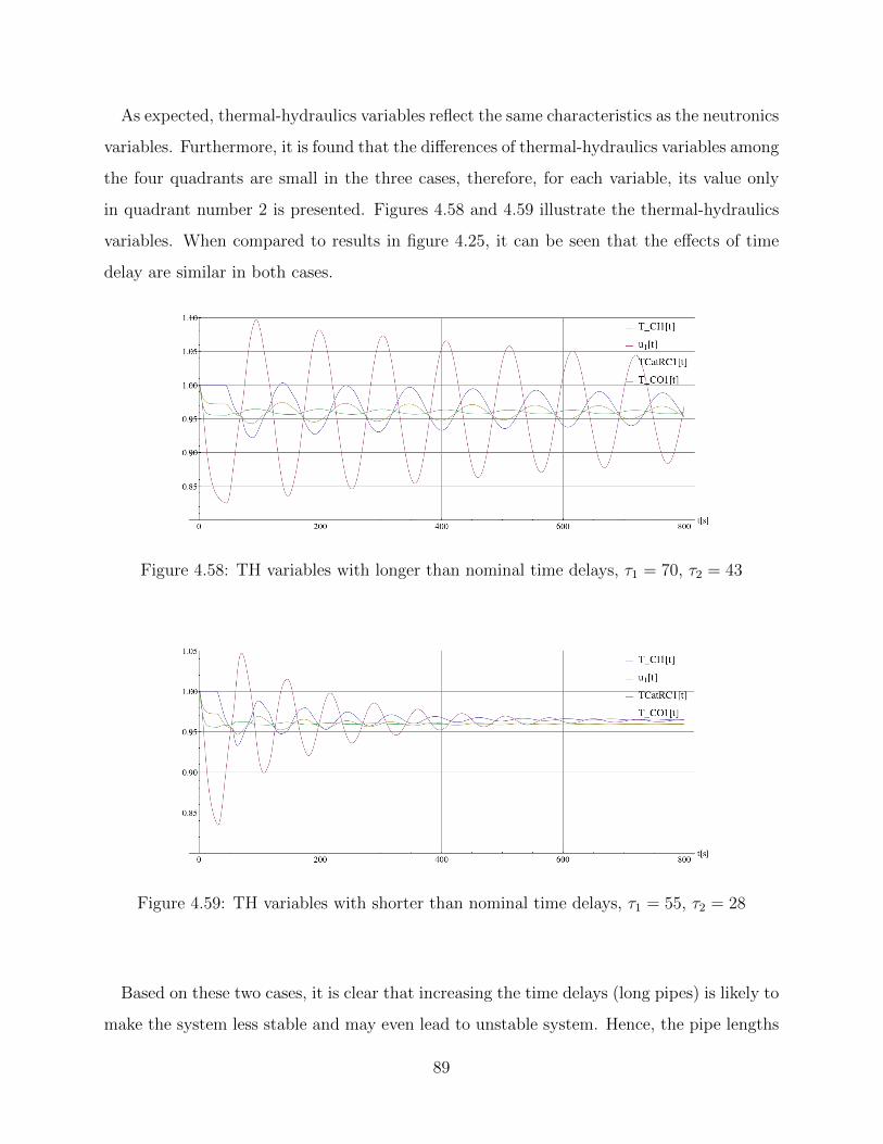
As expected, thermal-hydraulics variables reflect the same characteristics as the neutronics

variables. Furthermore, it is found that the differences of thermal-hydraulics variables among

the four quadrants are small in the three cases, therefore, for each variable, its value only

in quadrant number 2 is presented. Figures 4.58 and 4.59 illustrate the thermal-hydraulics

variables. When compared to results in figure 4.25, it can be seen that the effects of time

delay are similar in both cases.

Figure 4.58: TH variables with longer than nominal time delays, τ1 = 70, τ2 = 43

Figure 4.59: TH variables with shorter than nominal time delays, τ1 = 55, τ2 = 28

Based on these two cases, it is clear that increasing the time delays (long pipes) is likely to

make the system less stable and may even lead to unstable system. Hence, the pipe lengths

89

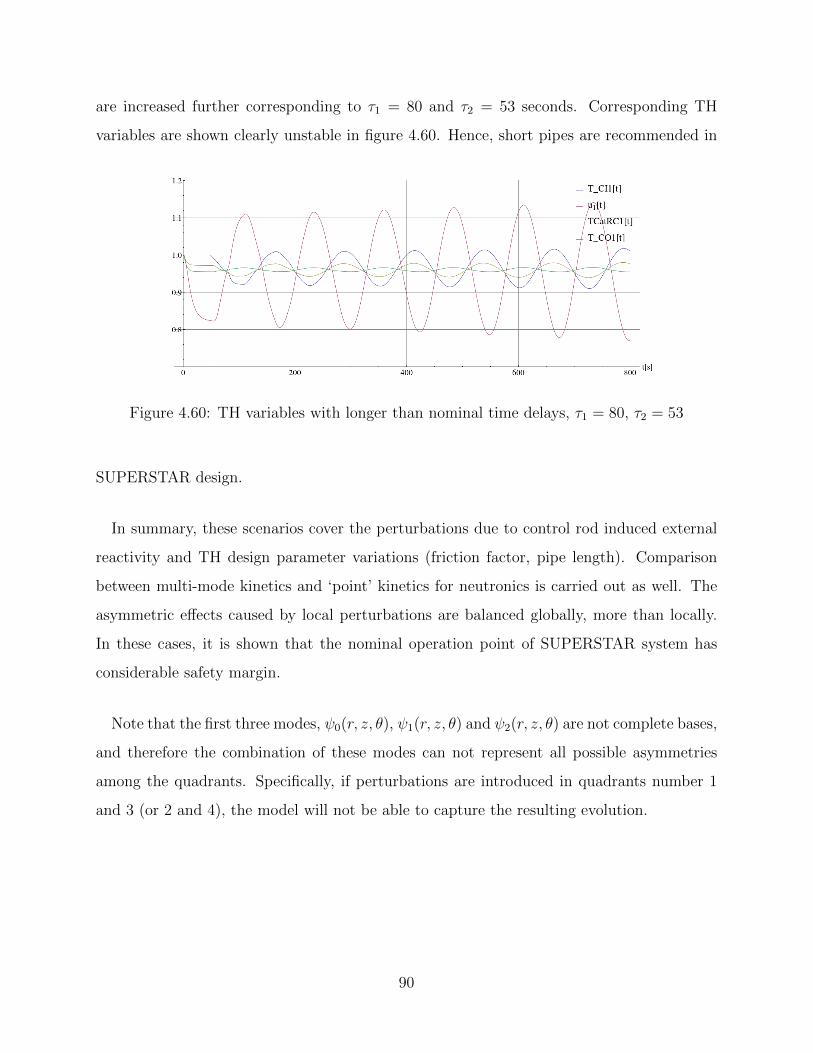
are increased further corresponding to τ1 = 80 and τ2 = 53 seconds. Corresponding TH

variables are shown clearly unstable in figure 4.60. Hence, short pipes are recommended in

Figure 4.60: TH variables with longer than nominal time delays, τ1 = 80, τ2 = 53

SUPERSTAR design.

In summary, these scenarios cover the perturbations due to control rod induced external

reactivity and TH design parameter variations (friction factor, pipe length). Comparison

between multi-mode kinetics and ‘point’ kinetics for neutronics is carried out as well. The

asymmetric effects caused by local perturbations are balanced globally, more than locally.

In these cases, it is shown that the nominal operation point of SUPERSTAR system has

considerable safety margin.

Note that the first three modes, ψ0(r, z, θ), ψ1(r, z, θ) and ψ2(r, z, θ) are not complete bases,

and therefore the combination of these modes can not represent all possible asymmetries

among the quadrants. Specifically, if perturbations are introduced in quadrants number 1

and 3 (or 2 and 4), the model will not be able to capture the resulting evolution.

90

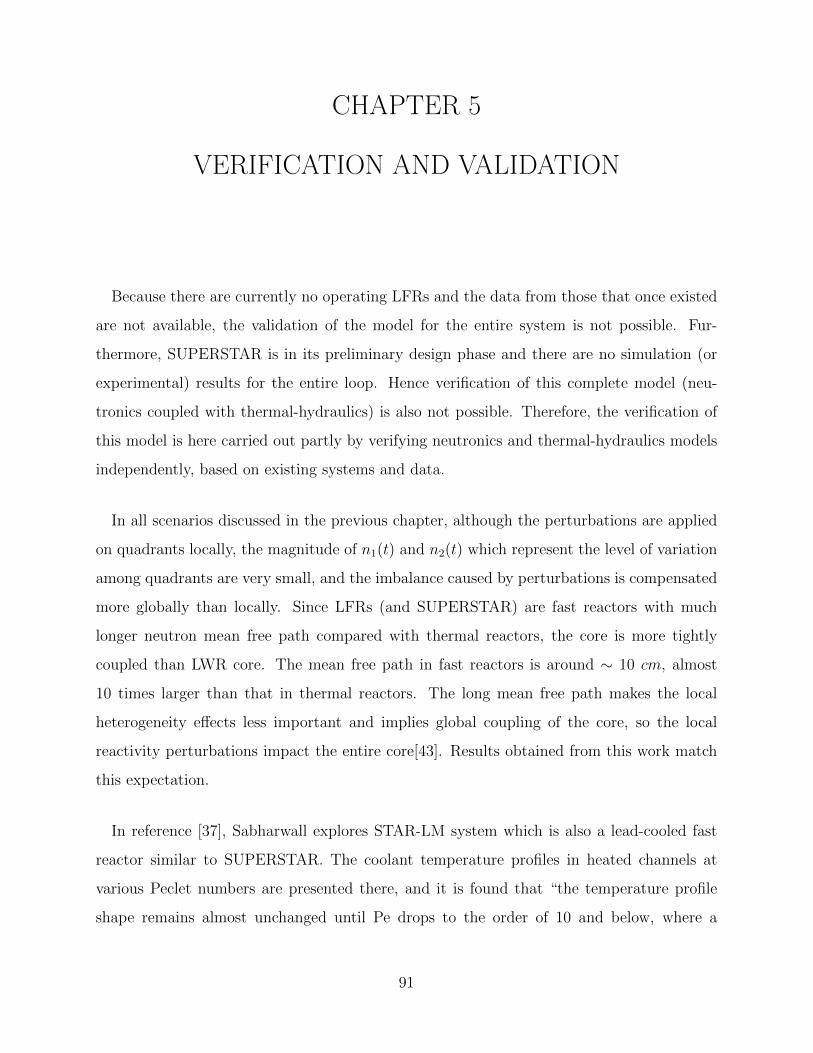
CHAPTER 5

VERIFICATION AND VALIDATION

Because there are currently no operating LFRs and the data from those that once existed

are not available, the validation of the model for the entire system is not possible. Fur-

thermore, SUPERSTAR is in its preliminary design phase and there are no simulation (or

experimental) results for the entire loop. Hence verification of this complete model (neu-

tronics coupled with thermal-hydraulics) is also not possible. Therefore, the verification of

this model is here carried out partly by verifying neutronics and thermal-hydraulics models

independently, based on existing systems and data.

In all scenarios discussed in the previous chapter, although the perturbations are applied

on quadrants locally, the magnitude of n1(t) and n2(t) which represent the level of variation

among quadrants are very small, and the imbalance caused by perturbations is compensated

more globally than locally. Since LFRs (and SUPERSTAR) are fast reactors with much

longer neutron mean free path compared with thermal reactors, the core is more tightly

coupled than LWR core. The mean free path in fast reactors is around ∼ 10 cm, almost

10 times larger than that in thermal reactors. The long mean free path makes the local

heterogeneity effects less important and implies global coupling of the core, so the local

reactivity perturbations impact the entire core[43]. Results obtained from this work match

this expectation.

In reference [37], Sabharwall explores STAR-LM system which is also a lead-cooled fast

reactor similar to SUPERSTAR. The coolant temperature profiles in heated channels at

various Peclet numbers are presented there, and it is found that “the temperature profile

shape remains almost unchanged until Pe drops to the order of 10 and below, where a

91

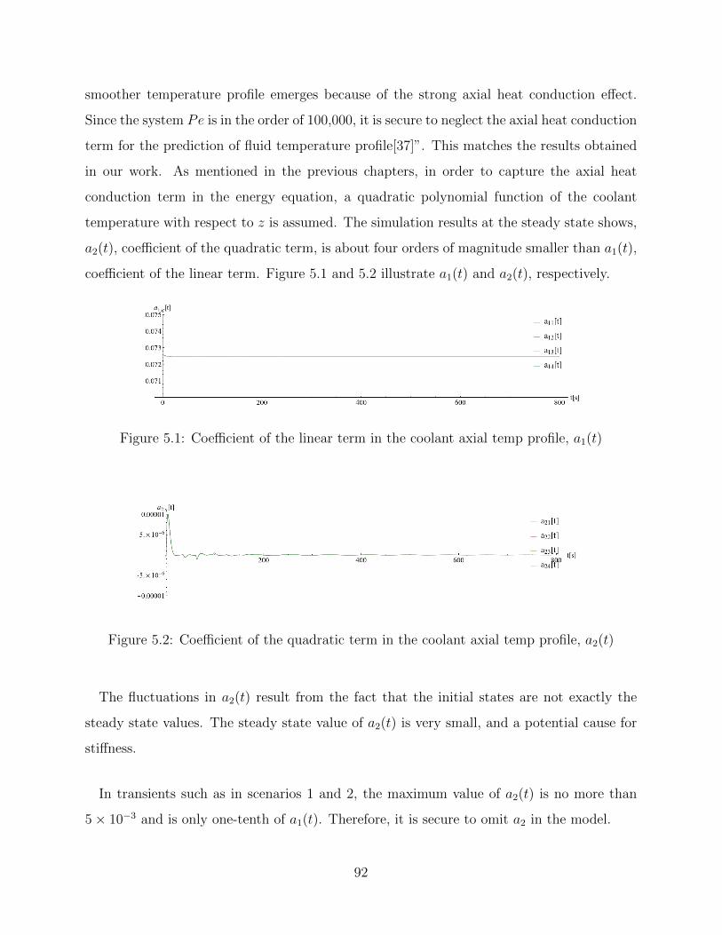
smoother temperature profile emerges because of the strong axial heat conduction effect.

Since the system Pe is in the order of 100,000, it is secure to neglect the axial heat conduction

term for the prediction of fluid temperature profile[37]”. This matches the results obtained

in our work. As mentioned in the previous chapters, in order to capture the axial heat

conduction term in the energy equation, a quadratic polynomial function of the coolant

temperature with respect to z is assumed. The simulation results at the steady state shows,

a2(t), coefficient of the quadratic term, is about four orders of magnitude smaller than a1(t),

coefficient of the linear term. Figure 5.1 and 5.2 illustrate a1(t) and a2(t), respectively.

Figure 5.1: Coefficient of the linear term in the coolant axial temp profile, a1(t)

Figure 5.2: Coefficient of the quadratic term in the coolant axial temp profile, a2(t)

The fluctuations in a2(t) result from the fact that the initial states are not exactly the

steady state values. The steady state value of a2(t) is very small, and a potential cause for

stiffness.

In transients such as in scenarios 1 and 2, the maximum value of a2(t) is no more than

5× 10−3 and is only one-tenth of a1(t). Therefore, it is secure to omit a2 in the model.

92

For the neutronics part, Bortot et. al.[3] present the reactivity coefficients for the core of

SUPERSTAR. The Dopper coefficient at the beginning of life cycle (BoL) is −0.55 pcm/K.

In this work, the slopes of the linear relation between Σ∗f , Σ∗a and the fuel temperature are rep-

resented by∂Σf

∂Tand ∂Σa

∂T. They are −6.9333×10−7 1/m per K and 8.6667×10−7 1/m per K,

respectively, as shown in table B.1. Now for 1 K change in the fuel average temperature,

the change in the term −Σa + (1− βe) · νΣf in reactivity matrix is then

−∂Σa

∂T+ (1− βe) · ν

∂Σf

∂T= −2.7346× 10−6 1/m (5.1)

As discussed previously, 1% control rod contribution corresponds to an equivalent Σa value

of 5.9274 × 10−4 1/m, and introduces a negative reactivity value of 13 cents. After scaling

by ΦΦΦ−1 ·∫QW Tψψψ∗d3rrr∗ term in equation (2.15), its equivalent contribution to the coefficient

of n(t)n(t)n(t) term is −1.4818 × 10−4 1/m, which corresponds to 13 cents of negative reactivity,

i.e., −27.95 pcm.

Therefore the reactivity induced by 1 K change in the fuel temperature

−27.95

−1.4818× 10−4/− 2.7346× 10−6= −0.51581 (pcm) (5.2)

This result shows that 1 K increase in fuel temperature introduces −0.51581 pcm of reac-

tivity. Compared with the data in reference[3], which is −0.55 pcm/K, the slopes describing

the linear relationship between cross sections and the fuel temperature are plausible.

93

CHAPTER 6

CONCLUSIONS AND FUTURE WORK

In this chapter, conclusions are presented first, followed by recommendations for future

work.

6.1 Conclusions

We studied the stability of natural circulation lead-cooled fast reactor system in Hcore−fwspace without neutronics coupling in section 4.1, in both frequency and time domains. In

general, with the nominal parameter values, the natural circulation system is considerably

stable and the nominal operation point is far away from the stability boundary. Based on

the simulations carried out in this work, a larger reactor core height has a negative impact on

system stability. A larger friction factor in the loop have a positive impact on flow stability,

however, as expected, it deteriorates the natural circulation performance.

The forced circulation system studied here is rather straightforward. It shows plausible

results and the system, as expected, is very robust.

For the natural circulation system with coupled neutronics and thermal-hydraulics, eight

scenarios are explored and presented in section 4.3. The first three scenarios focus on the

stability of the system due to perturbations in the control rod induced external reactivity.

When negative or positive reactivities are inserted into different quadrants, the local az-

imuthal effects can be observed. These azimuthal asymmetries are not significant in these

three scenarios. Furthermore, thermal hydraulics variables are all within allowed limita-

tions even when the reactor is operating at ∼ 135% of the nominal power level. Scenario

94

5 illustrates the system evolution due to blockages (represented by friction factor) in two

loops (quadrants). It is shown that with blockages introduced in two quadrants, the power

levels in the four quadrants remain nearly at the same level. Thus the large difference in

coolant velocity among loops does not have significant impact on neutronics. The effect of

design parameters such as pipe lengths are explored in scenario 7, and the results show that

shorter pipe lengths have positive impact on the system stability. Thus, by increasing the

pipe lengths, it is possible to make the system unstable. Therefore, shorter pipes between

thermal centers are recommended in SUPERSTAR design. Scenario 8 compares the model

with multi-mode kinetics and the model with ‘point’ kinetics, and it confirms the same

conclusions as drawn from the first three scenarios.

6.2 Future work

Doppler feedback effect in this work is described by a linear dependence of macroscopic

cross sections on temperature. However, the dependency between fuel temperature and cross

sections is not always linear. Specifically, when analyzing scenarios that lead to large changes

in fuel temperatures, better models for Doppler broadening effect should be employed. Neu-

tronics model can also be extended to allow azimuthally asymmetric perturbations that are

expected to lead to sin(2θ) and/or cos(2θ) variations.

Biggest limitations in the TH model of the loop is the simplified balance of plant model.

Once better design parameter are known, improved models for flow between core exit and

core inlet can be introduced. Even the simple delayed effect TH model can be improved by

treating the two delays in the model (τ1 and τ2) as a function of coolant velocity (and hence,

time).

In this work, all perturbations, including the control rod movements, blockages and coolant

temperature variations, are applied on the system through delta or step functions. However,

practically, these perturbations are usually more smooth. These should be addressed in

future work.

95

APPENDIX A

ATTRIBUTES OF SUPERSTAR

Attributes of the SUPERSTAR design[2]:

• Small (<300 MWe) and medium (300 to 700 MWe) sized reactors are better suited to

growing economies and to infrastructures of developing nations than classical economy-

of-scale plants. They can be deployed in increments, with each reactor constructed in

a shorter time than economy-of-scale plants, enabling planning and financing to be

spread out over time;

• They are right sized for initially small but fast growing electric grids for which changes

in load demand can be significant. Small and medium sized reactors provide greater

base load flexibility;

• SUPERSTAR can be readily transported and assembled from transportable modules;

• The initial fissile inventory is large but the one-time initial fissile loading is less than

the lifetime U-235 consumption of a Light Water Reactor (LWR) for same energy

delivery;

• Once loaded, STARs are fissile self sufficient with a conversion ratio, CR ∼ 1.0, which

provides proliferation resistance. Access to fuel is restricted. SUPERSTAR does not

incorporate any in-vessel fuel handling equipment. There is no on-site refueling equip-

ment. Refueling equipment is brought on-site only at the time of refueling after which

it is removed. The long core lifetime further restricts access to fuel by reducing or com-

pletely eliminating the need for refueling. The design restricts the potential for misuse

in a breeding mode. The fuel form is unattractive in a safeguards sense by virtue of

high radioactivity due to incomplete removal of fission products during reprocessing;

96

• SUPERSTAR incorporates autonomous load following and a S-CO2 Brayton cycle

power converter with a control strategy facilitating autonomous load following by the

reactor[2]. It is not necessary for operators to change the reactor power through delib-

erate motion of control rods. The control rods are mainly for startup and shutdown as

well as slow compensation of the burn-up reactivity swing over the core lifetime. This

supports the goal of making SUPERSTAR simple to operate, reducing operating staff

requirements and providing high reliability;

• They provide energy security for nations not wanting the expense of an indigenous

fuel cycle and waste repository infrastructure but willing to accept the guarantee of

services from a regional fuel cycle center by virtue of a long (15- to 30-year) refueling

interval;

• Low pressure liquid metal coolant with a high boiling temperature eliminates chance

of flashing of coolant;

• Type of vessel configuration with a guard vessel eliminates chance of loss-of-coolant;

• A high level of passive safety, reducing the number of accident initiators and the need

for safety systems, enabling the size of the exclusion and emergency planning zones to

potentially be reduced;

• Natural circulation primary coolant heat transport at any power level up to and ex-

ceeding full power, which eliminates pump-related accidents;

97

APPENDIX B

DIMENSIONLESS VARIABLES AND SUPERSTARPARAMETER VALUES

This appendix lists dimensionless variables. Reference values used in this work are:

L∗ref = 1 m, reference length

v∗ref = 1 m/s, reference velocity

T ∗ref = (400.0 + 273.15) K = 673.15 K, reference temperature

n∗ref = n∗ at nominal steady state.

n∗ref represents the value of the time-dependent term n∗(t) at the nominal steady-state.

At the steady state, only fundamental mode is retained. Thus, we have

E0 · v∗ ·∫dV

ψ0(r∗r∗r∗) · n∗ref · Σf = 300MWth (B.1)

Where E0 is the energy emitted per fission which is approximately equal to 200 MeV .

v∗ is the neutron speed corresponding to 2 MeV kinetic energy, Σf is the corresponding

macroscopic fission cross section at the average temperature, which is interpolated from

SERPENT calculations, ψ0(r∗r∗r∗) is the shape function for the fundamental mode and the

integral is over the whole volume of the reactor core. Then, n∗ref is solved from equation

(B.1).

With these reference values, dimensional parameters can be converted to their dimension-

less form as below:

ri =r∗iL∗ref

, i = p, g, c (p: pellet, g:gap, c:clad)

t =t∗v∗refL∗ref

v = v∗

v∗ref

αp =k∗p/(ρ

∗pC∗p )

L∗refv∗ref

98

αc = k∗c/(ρ∗cC∗c )

L∗refv∗ref

nk(t) =n∗k(t∗)

n∗ref, k = 0, 1, 2

cq =c∗qn∗refL

∗ref

2

k∗pT∗ref

Bic = h∗∞r∗c

k∗c

Big =h∗gr∗g

k∗c

Bip =h∗gr∗g

k∗p

The SUPERSTAR design and operating parameters used[1][2][26][27][29] in this work are

listed in table B.1.

99

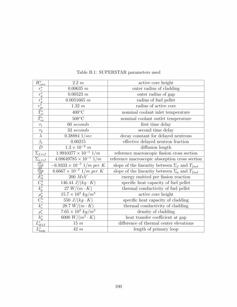
Table B.1: SUPERSTAR parameters used

H∗core 2.2 m active core heightr∗c 0.00635 m outer radius of claddingr∗g 0.00523 m outer radius of gap

r∗p 0.0051665 m radius of fuel pellet

r∗ac 1.32 m radius of active core

T ∗ci 400◦C nominal coolant inlet temperature

T ∗co 508◦C nominal coolant outlet temperatureτ1 60 seconds first time delayτ2 33 seconds second time delayλ 0.38884 1/sec decay constant for delayed neutronsβe 0.00215 effective delayed neutron fractionD 1.3× 10−2 m diffusion length

Σf,ref 1.9910377× 10−1 1/m reference macroscopic fission cross sectionΣa,ref 4.08649785× 10−1 1/m reference macroscopic absorption cross section∂Σf

∂T−6.9333× 10−7 1/m per K slope of the linearity between Σf and Tfuel

∂Σa

∂T8.6667× 10−7 1/m per K slope of the linearity between Σa and Tfuel

E∗0 200 MeV energy emitted per fission reactionC∗p 146.44 J/(kg ·K) specific heat capacity of fuel pellet

k∗p 27 W/(m ·K) thermal conductivity of fuel pellet

ρ∗p 15.7× 103 kg/m3 active core height

C∗c 550 J/(kg ·K) specific heat capacity of claddingk∗c 28.7 W/(m ·K) thermal conductivity of claddingρ∗c 7.65× 103 kg/m3 density of claddingh∗g 6000 W/(m2 ·K) heat transfer coefficient at gap

L∗diff 15 m difference of thermal center elevations

L∗loop 42 m length of primary loop

100

APPENDIX C

DERIVATION OF THE FUEL PIN HEATCONDUCTION EQUATION

This appendix shows the derivation of equations describing fuel pins heat conduction pro-

cess for natural circulation loop coupled with neutronics. The goal of this derivation is to

link the energy equations with neutronics equations. Furthermore, at the end of this ap-

pendix, the fuel pins heat conduction models for natural circulation system without coupled

neutronics and for forced circulation (open loop) system are discussed.

In the coolant energy equations, the heat source term q∗′′′e (t) is related to the heat convec-

tion process taking place on the surface of the fuel pin cladding while this heat convection

process is determined by the time-dependent fuel pin cladding surface temperature TCatRC

and the coolant bulk temperature Tbulk(t). On the other hand, in the fuel pins heat conduc-

tion model, its heat source term q∗′′′c (t) is directly related to the fission reactions which are

described by the variables n0(t), n1(t) and n2(t). Therefore, the neutronics part is ultimately

connected with the coolant energy equation through this fuel pin heat conduction model.

The schematic graph of the fuel pin in SUPERSTAR is presented in figure C.1 where

the fuel pellet, 0 < r∗ < r∗p, the gap, r∗p < r∗ < r∗g , and the cladding, r∗g < r∗ < r∗c are

illustrated. SUPERSTAR incorporates an innovative particulate metallic fuel in which after

a short irradiation period, the fuel will swell radially outward and come into contact with the

inner surface of the cladding[27]. Without losing generality, the gap model is still included

in this work.

For the sake of simplicity, we take the assumption that fuel pins have uniform temperature

distributions in the axial and in the azimuthal directions, and the temperature distribution

obeys a quadratic profile only with respect to r. For a single fuel pellet, its temperature at

101

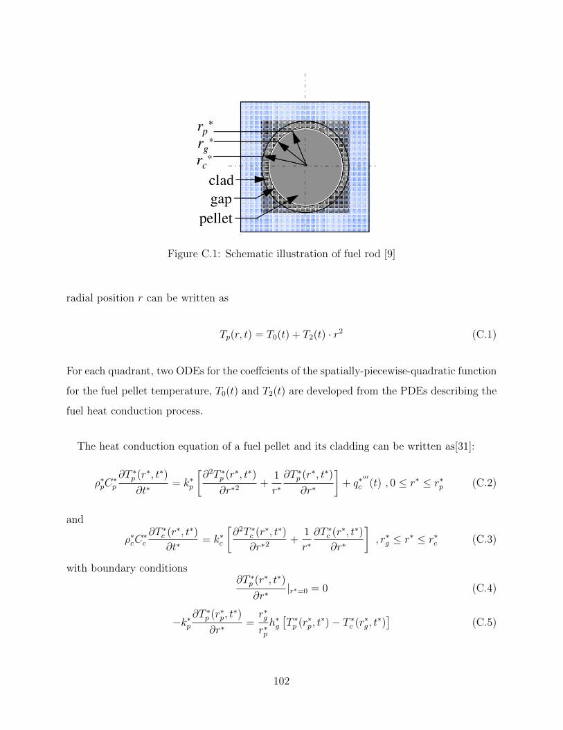
Figure C.1: Schematic illustration of fuel rod [9]

radial position r can be written as

Tp(r, t) = T0(t) + T2(t) · r2 (C.1)

For each quadrant, two ODEs for the coeffcients of the spatially-piecewise-quadratic function

for the fuel pellet temperature, T0(t) and T2(t) are developed from the PDEs describing the

fuel heat conduction process.

The heat conduction equation of a fuel pellet and its cladding can be written as[31]:

ρ∗pC∗p

∂T ∗p (r∗, t∗)

∂t∗= k∗p

[∂2T ∗p (r∗, t∗)

∂r∗2+

1

r∗∂T ∗p (r∗, t∗)

∂r∗

]+ q∗

′′′

c (t) , 0 ≤ r∗ ≤ r∗p (C.2)

and

ρ∗cC∗c

∂T ∗c (r∗, t∗)

∂t∗= k∗c

[∂2T ∗c (r∗, t∗)

∂r∗2+

1

r∗∂T ∗c (r∗, t∗)

∂r∗

], r∗g ≤ r∗ ≤ r∗c (C.3)

with boundary conditions∂T ∗p (r∗, t∗)

∂r∗|r∗=0 = 0 (C.4)

−k∗p∂T ∗p (r∗p, t

∗)

∂r∗=r∗gr∗ph∗g[T ∗p (r∗p, t

∗)− T ∗c (r∗g , t∗)]

(C.5)

102

−k∗c∂T ∗c (r∗g , t

∗)

∂r∗= h∗g

[T ∗p (r∗p, t

∗)− T ∗c (r∗g , t∗)]

(C.6)

−k∗c∂T ∗c (r∗c , t

∗)

∂r∗= h∗∞ [T ∗c (r∗c , t

∗)− T ∗bulk(t)] (C.7)

where the convective heat transfer coefficient h∗∞ on the fuel cladding surface is estimated

by Dittus-Boelter correlation. q∗′′′c (t∗), that couples the neutronics to the heat conduction

model, is the time-dependent volumetric heat generation rate in the fuel pellet due to the

fission reactions, with units of J/(m3 · s). It links the fission reaction rate R∗(t∗) and thus,

the terms n0(t), n1(t) and n2(t), to the heat conduction model. The physical meanings of

other symbols in the above equations can be found in Appendix B.

The first step of this derivation is to identify the relation between q∗′′′c (t∗) and n0(t), n1(t)

and n2(t). With the assumption that, even in transients, the fission cross section remains

the same across the whole volume as its steady-state value, the volumetric reaction rate can

be written as

R∗(rrr∗, t∗) = Σ∗f · φ∗(rrr∗, t∗) (C.8)

This assumption is only valid if no feedback is taken into account. Cross sections are actually

functions of fuel temperature when feedback effects are considered. Doing the volumetric

averaging over one quadrant, we have

R∗q(t∗) =

Σ∗fV ∗q·∫Vq

φ∗(rrr∗, t∗)dV (C.9)

where V ∗q is the volume of one quadrant of the reactor core. R∗q(t∗) is the averaged volumetric

reaction rate for this quadrant.

The neutron flux can be expressed by retaining the first three modes as:

φ∗(r∗, t∗) = v∗ ·2∑j=0

ψ∗j (r∗)n∗j(t

∗) (C.10)

103

Assuming E∗0 is the energy released from one fission reaction, then the heat generation rate

within one quadrant for the homogeneous reactor is

q∗′′′

h (t∗) = E∗0 ·R∗q(t∗) =E∗0 · Σ∗fV ∗q

∫Vq

φ∗(r∗, t∗)dV

=E∗0 · Σ∗f · v∗

V ∗q

∫Vq

[ψ∗0(r∗)n∗0(t∗) + ψ∗1(r∗)n∗1(t∗) + ψ∗2(r∗)n∗2(t∗)] dV

=E∗0 · Σ∗f · v∗

V ∗q

∫Vq

ψ∗0(r∗) · n∗0(t∗)dV

+E∗0 · Σ∗f · v∗

V ∗q

∫Vq

ψ∗1(r∗) · n∗1(t∗)dV

+E∗0 · Σ∗f · v∗

V ∗q

∫Vq

ψ∗2(r∗) · n∗2(t∗)dV

(C.11)

In order to capture the asymmetry of power levels among quadrants, the integral in the

above equation is taken over quadrants rather than the whole core volume. Furthermore,

considering the heat generation only takes place in the fuel pins, the heat generation rate

q∗′′′c (t) appearing in equation (C.2) is scaled from q∗

′′′

h (t∗) by a factor which accounts for the

volume difference between fuel pins in one quadrant and one homogeneous reactor quadrant.

Thus,

q∗′′′

c (t) =V ∗qV ∗f· q∗′′′h (t) = c∗qn

∗0(t∗) + c∗qζ1n

∗1(t∗) + c∗qζ2n

∗2(t∗) (C.12)

where V ∗f is the volume of all fuel pins in one quadrant.

c∗q =E∗0 · Σ∗f · v∗

V ∗f

∫Vq

ψ∗0(rrr∗)dV (C.13)

ζ1 and ζ2 are dimensionless normalization factors and they are defined as

ζ1 =(1, ψ∗1(rrr∗))V ∗q(1, ψ∗0(rrr∗))V ∗q

, ζ2 =(1, ψ∗2(rrr∗))V ∗q(1, ψ∗0(rrr∗))V ∗q

(C.14)

where (a, b)V ∗q means the volume integral over the quadrant for the product of a and b.

Because the first and second modes have symmetric profile over each quadrant, these factors

have the same absolute value, but the signs vary for different quadrants.

104

The second step is to find the dimensionless form of these equations. With reference

constants (T ∗ref , v∗ref , n

∗ref , L

∗ref , etc.), and by plugging equation (C.12) into equations (C.2–

C.7), they can be transformed to their dimensionless form

1

αp

∂Tp(r, t)

∂t=

[∂2Tp(r, t)

∂r2+

1

r

∂Tp(r, t)

∂r

]+ cqn0(t) + cqζ1n1(t) + cqζ2n2(t),

0 ≤ r ≤ rp

(C.15)

1

αc

∂Tc(r, t)

∂t=∂2Tc(r, t)

∂r2+

1

r

∂Tc(r, t)

∂r, rg ≤ r ≤ rc (C.16)


∂r|r=0 = 0 (C.17)

−∂Tp(rp, t)∂r

=Biprp

[Tp(rp, t)− Tc(rg, t)] (C.18)

−∂Tc(rg, t)∂r

=Bigrg

[Tp(rp, t)− Tc(rg, t)] (C.19)

−∂Tc(rc, t)∂r

=Bicrc

[Tc(rc, t)− Tbulk(t)] (C.20)

where Tbulk(t) is the bulk temperature of coolant and evaluated as [Tco(t) + Tci(t)] /2. Tco(t)

and Tci(t) are the dimensionless coolant temperatures at the core outlet and inlet, respec-

tively.

Before applying the weighted residual method to convert these PDEs to ODES, the third

step is carried out to express Tc(r, t) in terms of Tp(r, t) and Tbulk(t), which eliminates

equation (C.16) and reduces the boundary condition equations (C.18,C.19,C.20) into one

equation by establishing the heat convection boundary conditions on the basis of Tp(r, t)

and Tbulk(t) directly.

In this step, it is necessary to find out the steady state solution first. At the steady

state, only the fundamental mode in neutronics is retained and represented by n0 here.

Furthermore, the reference constant n∗ref has been chosen as n∗0, therefore, n0 = 1.

105

Tp(r), Tc(r) are steady-state solutions satisfying

0 =

[∂2Tp(r)

∂r2+

1

r

∂Tp(r)

∂r

]+ cqn0, 0 ≤ r ≤ rp (C.21)

0 =∂2Tc(r)

∂r2+

1

r

∂Tc(r)

∂r, rg ≤ r ≤ rc (C.22)

with boundary conditions

∂Tp(r)

∂r|r=0 = 0 (C.23)

−∂Tp(rp)∂r

=Biprp

[Tp(rp)− Tc(rg)

](C.24)

−∂Tc(rg)∂r

=Bigrg

[Tp(rp)− Tc(rg)

](C.25)

−∂Tc(rc)∂r

=Bicrc

[Tc(rc)− Tbulk

](C.26)

where

Tbulk =Tco + Tci

2(C.27)

Tco and Tci are nominal coolant temperature at the core outlet and inlet in dimensionless

form, while their dimensional values are 508◦C and 400◦C, respectively[2].

Solving equations (C.21–C.26), we have

Tp(r) = −cqn0r2

4+ b1, 0 ≤ r ≤ rp (C.28)

Tc(r) = b2 log(r) + b3, rg ≤ r ≤ rc (C.29)

and

b1 = − b2

Big+ cqn0

r2p

4+ b2 log(rg) + b3 (C.30)

b2 = −cqn0BigBip

r2p

2(C.31)

106

b3 = − b2

Bic− b2 log(rc) + Tbulk (C.32)

Because the thermal diffusivity in fuel pin claddings α∗c is large and during a transient

there is no significant change in the cladding temperature profile from its initial steady-state

distribution. Thus, we use the steady-state cladding temperature distribution and use the

boundary condition equations (C.19) and (C.20) for claddings to arrive at an approximate

expression for the cladding temperature Tc(r, t) in transients, which appears in the energy

equation of the coolant. Now, by setting

Tc(r, t) = b2(t) log(r) + b3(t), rg ≤ r ≤ rc (C.33)

and substituting the above equation into equation (C.16), with boundary condition eqautions

(C.19) and (C.20), we have

b2(t) =−BigBic


)Tp(rp, t)

+BigBic


)Tbulk(t)

(C.34)

b3(t) =Big +BigBic log(rc)


)Tp(rp, t)

+Bic −BicBig log(rg)


)Tbulk(t)

(C.35)

Evaluating Tc(r, t) at r = rg,

Tc(rg, t) =Big +BigBic log( rc

rg)


)Tp(rp, t)

+Bic


)Tbulk(t)

(C.36)

107

Substituting this expression into equation (C.18), we have

−∂Tp(rp, t)∂r

=Biprp

BicBig +Bic +BigBic log( rc

rg)Tp(rp, t)

−Biprp

BicBig +Bic +BigBic log( rc

rg)Tbulk(t)

=Bi+prp

Tp(rp, t)−Bi+prp

Tbulk(t)

(C.37)

where

Bi+p = BipBic


)(C.38)

is the modified Biot number.

Now we have the strong form of the PDEs

1

αp

∂Tp(r, t)

∂t=

[∂2Tp(r, t)

∂r2+

1

r

∂Tp(r, t)

∂r

]+cqn0(t)+cqζ1n1(t)+cqζ2n2(t), 0 ≤ r ≤ rp (C.39)


∂r|r=0 = 0 (C.40)

−∂Tp(rp, t)∂r

=Bi+prp

[Tp(rp, t)− Tbulk(t)] (C.41)

The fuel pellet temperature and the coolant bulk temperature are linked directly and ex-

plicitly in boundary condition (C.41).

The fourth step is to convert above the PDE to ODEs. The weighted residual method is

used here. With

Tp(r, t) = T0(t) + T2(t)r2 (C.42)

the basis functions are r0 and r2, hence the trial functions are chosen as r0 and r2. Further-

more, the boundary condition (C.40) is also satisfied at the outset.

108

In the context of weighted residual method, equations (C.39) and (C.41) can be written

as

ATp − fA = 0 (C.43)

and

BTp − fB = 0 (C.44)

where,

A =1

αp

∂

∂t− ∂2

∂r2− 1

r

∂

∂r, fA = cqn0(t) + cqξ1n1(t) + cqξ2n2(t) (C.45)

B = − ∂

∂r|r=rp , fB =

Bi+prp

[Tp(rp, t)− Tbulk(t)] (C.46)

We form the equations

(1, ATp − fA) + (1, BTp − fB) = 0 (C.47)

(r2, ATp − fA) + (r2, BTp − fB) = 0 (C.48)

(a, b) means doing the integral over the appropriate domain or boundary for the product of

a and b. After rearranging, we have

1

αp

[dT0(t)

dtrp +

dT2(t)

dt

r3p

3

]− 4T2(t)rp − fArp − 2T2(t)rp − fB = 0 (C.49)

1

αp

[dT0(t)

dt

rp3

+dT2(t)

dt

r3p

5

]− 4T2(t)

rp3− fA

rp3− 2T2(t)rp − fB = 0 (C.50)

As we have known, Tbulk(t) is defined by

Tbulk(t) =Tco(t) + Tci(t)

2(C.51)

From the heat exchanger model in chapter 3, we know that

Tci(t) = p00 + p10 · Tco(t− τ1) + p01 · u(t− τ2) (C.52)

109

where u(t) is the dimensionless coolant flow velocity, and τ1 and τ2 represent the time delays

in the loop. From the coolant energy equation, we know that

Tco(t) = Tci + a1(t) ·H + a2(t) ·H2 (C.53)

where H is the non-dimensional reactor active core height. Therefore, Tbulk(t) can be ex-

pressed as a function of a1(t− τ1), a2(t− τ1) and u(t− τ2). These variables with time delays

render equations (3.49) and (3.50) to be DDEs for the coefficients T0(t) and T2(t) in the fuel

pellet temperature expression.

For the natural circulation system without coupling with the neutronics, a constant heat

generation rate replaces the heat source term q∗′′′c (t) in equation (C.2) while the other parts

remain the same. This constant is evaluated at the nominal steady state of the reactor core.

Because this system still incorporates the time delay effects in its closed loop, it is ultimately

described by DDEs as well. These DDEs have the same form as equations (3.49) and (3.50)

and the only update is to replace fA with the dimensionless constant heat generation rate.

For the forced circulation system, constant external pressure drop boundary condition is

applied on the core inlet and outlet. The same constant heat generation rate is assumed for

this system as in the natural circulation system without coupled neutronics. The coolant

temperature at the reactor core inlet is specified to be constant. This is an open loop therefore

no time delay effects are considered. The fuel pins heat conduction model in this system is

described by a set of ODEs. These ODEs have the same form as equations (3.49) and (3.50)

and the updates include replacing fA with the dimensionless constant heat generation rate

and replacing fB with the specified constant coolant inlet temperature.

110

APPENDIX D

DERIVATION OF THE MOMENTUM EQUATION

This appendix shows the derivation of the momentum equations of the coolant flow, and

has 2 parts. The first part discusses the momentum equation representing the natural

circulation coolant flow, which is valid for both the system with coupled neutronics and the

system without coupled neutronics. The second one discusses the forced circulation coolant

flow where fixed pressure drop boundary conditon is applied across the inlet and outlet of

the core. In both systems, Boussinesq approximation is assumed to be valid and hence

the coolant density can be treated as a constant except in the gravity term. Furthermore,

this approximation also implies that the other properties (such as k, Cp) of the coolant are

constant, and this point will be reiterated in the conservation of energy equations later in

Appendix E. This derivation follows similar approaches in reference[35][34].

The momentum equation for the natural circulation flow

The conservation of momentum equation along the 1-D flow path is

ρ∗du∗

dt∗= −∂p

∗

∂z∗− ρ∗(z∗, t∗)g∗z − f ∗w

1

2ρ∗ [u∗(t∗)]2 (D.1)

where ρ is the coolant density evaluated at the nominal average temperature, and f ∗w is a

lumped dimensional friction factor. Because SUPERSTAR is still in its preliminary design

stage, at this point, f ∗w is not known. Hence, it is calculated by parameterizing the equation

at the steady state point and then solving for f ∗w to ensure that the coolant velocity u∗ is

equal to its nominal value.

111

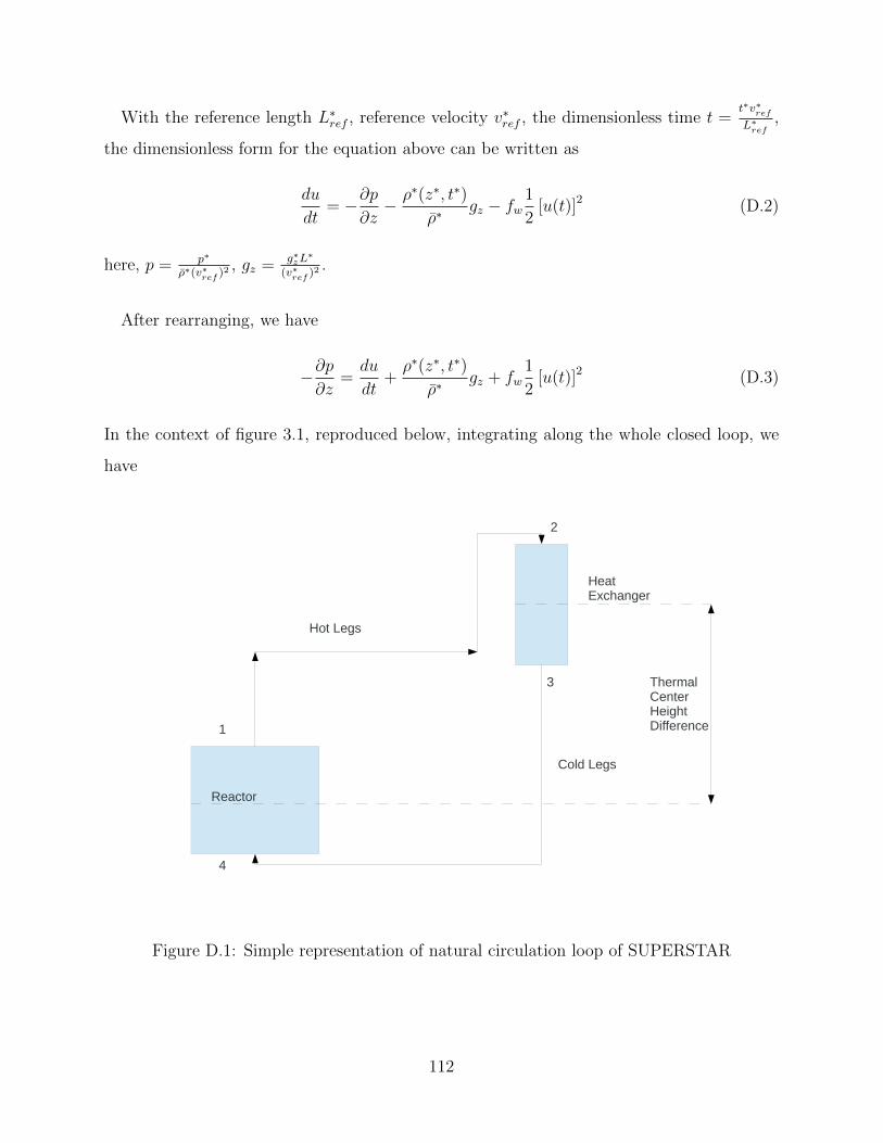
With the reference length L∗ref , reference velocity v∗ref , the dimensionless time t =t∗v∗refL∗ref

,

the dimensionless form for the equation above can be written as

du

dt= −∂p

∂z− ρ∗(z∗, t∗)

ρ∗gz − fw

1

2[u(t)]2 (D.2)

here, p = p∗

ρ∗(v∗ref )2, gz = g∗zL

∗

(v∗ref )2.

After rearranging, we have

−∂p∂z

=du

dt+ρ∗(z∗, t∗)

ρ∗gz + fw

1

2[u(t)]2 (D.3)

In the context of figure 3.1, reproduced below, integrating along the whole closed loop, we

have

4

1

3

2

Hot Legs

Cold Legs

Reactor

HeatExchanger

Thermal CenterHeightDifference

Figure D.1: Simple representation of natural circulation loop of SUPERSTAR

112

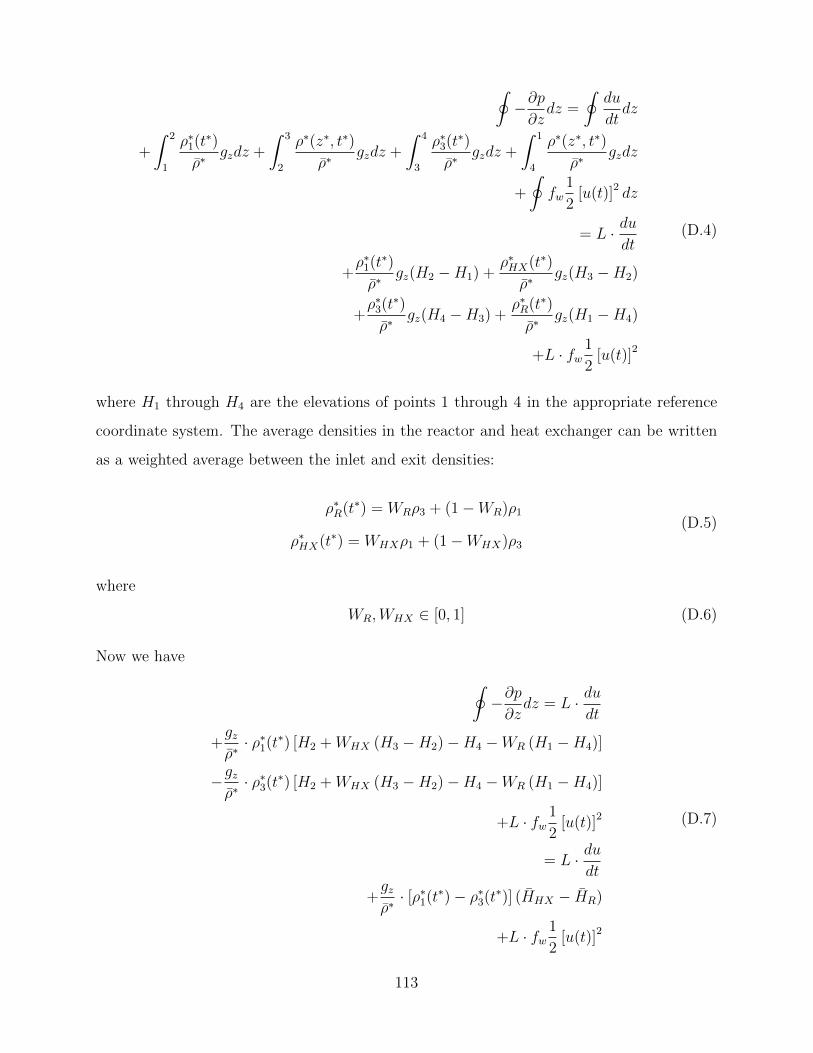
∮−∂p∂zdz =

∮du

dtdz

+

∫ 2

1

ρ∗1(t∗)

ρ∗gzdz +

∫ 3

2

ρ∗(z∗, t∗)

ρ∗gzdz +

∫ 4

3

ρ∗3(t∗)

ρ∗gzdz +

∫ 1

4

ρ∗(z∗, t∗)

ρ∗gzdz

+

∮fw

1

2[u(t)]2 dz

= L · dudt

+ρ∗1(t∗)

ρ∗gz(H2 −H1) +

ρ∗HX(t∗)

ρ∗gz(H3 −H2)

+ρ∗3(t∗)

ρ∗gz(H4 −H3) +

ρ∗R(t∗)

ρ∗gz(H1 −H4)

+L · fw1

2[u(t)]2

(D.4)

where H1 through H4 are the elevations of points 1 through 4 in the appropriate reference

coordinate system. The average densities in the reactor and heat exchanger can be written

as a weighted average between the inlet and exit densities:

ρ∗R(t∗) = WRρ3 + (1−WR)ρ1

ρ∗HX(t∗) = WHXρ1 + (1−WHX)ρ3

(D.5)

where

WR,WHX ∈ [0, 1] (D.6)

Now we have ∮−∂p∂zdz = L · du

dt

+gzρ∗· ρ∗1(t∗) [H2 +WHX (H3 −H2)−H4 −WR (H1 −H4)]

−gzρ∗· ρ∗3(t∗) [H2 +WHX (H3 −H2)−H4 −WR (H1 −H4)]

+L · fw1

2[u(t)]2

= L · dudt

+gzρ∗· [ρ∗1(t∗)− ρ∗3(t∗)] (HHX − HR)

+L · fw1

2[u(t)]2

(D.7)

113

where HHX = H2 + WHX(H3 − H2) and HR = H4 + WR(H1 − H4) are the elevations of

thermal centers within the heat exchanger and the core, respectively. In this work, we set

both WHX and WR equal to 0.5.

Substituting the equation of state into the equation above

ρ∗(t∗) = 11367− 1.1944 · T ∗(t∗) (D.8)

and recognizing that the intergral of the pressure gradient along the whole loop is zero, we

have

0 = L · dudt

+ Ldiff ·gz · Trefρ∗

· (−1.1944) · [T1(t)− T4(t)] + L · fw ·1

2[u(t)]2 (D.9)

where Ldiff is the vertical distance between the thermal centers of the reactor core and the

HX, and

T1(t) = Tco(t) = Tci + a1(t) ·H + a2(t) ·H2 (D.10)

is the time-dependent coolant temperature at the core outlet, and

T4(t) = Tci(t) = p00 + p10 · Tco(t− τ1) + p01 · u(t− τ2) (D.11)

is the time-dependent coolant temperature at the core inlet. p00, p10 and p01 are constants

to be determined by the HX model.

So far, the momentum equation for natural circulation scenario has been developed and

this is a DDE including a1(t− τ1), a2(t− τ1) and u(t− τ2).

The momentum equation for the forced circulation flow

Starting from the dimensionless momentum equation (3.4)

−∂p∂z

=du

dt+ρ∗(z∗, t∗)

ρ∗gz + fw ·

1

2[u(t)]2 (D.12)

114

and integrating from the inlet to the outlet of the heated channel, with the equation of state,

ρ∗(z∗, t∗) = 11367− 1.1944 · T ∗(z∗, t∗) (D.13)

we have

∆Pch =

∫ H

0

dzdu(t)

dt+H · 11367− 1.1944 ·

∫ H0T (z, t)dz · T ∗ref

ρ∗gz

+

∫ H

0

dz1

2fw [u(t)]2

(D.14)

Similar to the momentum equation derivation for natural circulation scenario, the coolant

temperature T (z, t) can be approximated by

T (z, t) = Tci + a1(t)z + a2(t)z2 (D.15)

Substituting equation (D.15) into equation (D.14), we have

∆Pch = H · du(t)

dt+H · 11367− 1.1944 · T ∗ref ·

[H · Tci + H2

2a1(t) + H3

3a2(t)

]ρ∗

gz

+H · 1

2fw [u(t)]2

(D.16)

In this forced circulation model, we assume, the pressure drop across the reactor core at the

steady state is half of the total pressure drop along the whole primary loop, i.e.

H · 1

2fw [u(t)]2 = 0.5 ·∆Ploop (D.17)

Thus, we have

∆Pch = H · du(t)

dt+H · 11367− 1.1944 · T ∗ref ·

[H · Tci + H2

2a1(t) + H3

3a2(t)

]ρ∗

gz

+0.5 ·∆Ploop

(D.18)

115

By ensuring the coolant velocity to be equal to its value at steady state, ∆Pch is specified.

Because this is an open loop and no HX model is included, therefore no time delay effects

are needed, and thus the above equation is an ODE for u(t).

116

APPENDIX E

DERIVATION OF THE ENERGY EQUATION

This appendix illustrates the derivation of the coolant energy equation and the steps to

develop ODEs from the corresponding PDEs. This follows similar method in reference[9].

The conservation of energy equation is

ρ∗C∗Pb(∂T ∗

∂t∗+ u∗

∂T ∗

∂z∗) = k∗Pb

∂2T ∗

∂z∗2+ q∗

′′′

e (E.1)

The volumetric heat generation rate q∗′′′e in this equation comes from the heat convection

process occuring on the fuel pin cladding surface. We have

q∗′′′

e = q∗′′P ∗

A∗(E.2)

Here, q∗′′

is the heat flux on the cladding surface, P ∗ is the dimensional wetted perimeter of

a single fuel pin cladding, A∗ is the dimensional cross sectional flow area of a single fuel pin

channel. Further rearranging equation (E.1), we have

∂T ∗

∂t∗+ u∗

∂T ∗

∂z∗= α∗Pb

∂2T ∗

∂z∗2+P ∗/A∗

ρ∗C∗Pbq∗′′

(E.3)

and its dimensionless form

∂T (z, t)

∂t+ u

∂T (z, t)

∂z= αPb

∂2T (z, t)

∂z2+P

Ah∞ [Tc(rc, t)− Tbulk(t)] (E.4)

where, P = P ∗/L∗, A = A∗/(L∗)2, αPb =α∗Pb

L∗v∗oand h∞ = h∗∞

ρ∗C∗Pbv∗o.

117

In the context of weighted residual method, the equation can be written as

BT − S = 0 (E.5)

Here

B =∂

∂t+ u

∂

∂z− αPb

∂2

∂z2(E.6)

S =P

Ah∞ [Tc(rc, t)− Tbulk(t)] (E.7)

The coolant temperature in the heated channels is given by T (z, t) = Tci + a1(t)z + a2(t)z2.

With the trial functions z0 and z1, two equations are formed

(1, BT − S) = 0 (E.8)

(z,BT − S) = 0 (E.9)

where, (a, b) means the integral of the inner product of a and b. Now we have

∫ H

0

dz

[da2(t)

dtz2 + (

da1(t)

dt+ u2a2(t))z + ua1(t)− αPb · 2a2(t)− P


]= 0

(E.10)

and∫ H

0

dz

[da2(t)

dtz3 + (

da1(t)

dt+ u2a2(t))z2 +

[ua1(t)− αPb · 2a2(t)− P


]z

]= 0

(E.11)

Integrating and rearranging the terms, we have

H

2

da1(t)

dt+H2

3

da2(t)

dt+H ·u·a2(t)+u·a1(t)−2αPba2(t)−P

Ah∞ [Tc(rc, t)− Tbulk(t)] = 0 (E.12)

118

and

2H

3

da1(t)

dt+H2

2

da2(t)

dt+

4H

3· u · a2(t) + u · a1(t)− 2αPba2(t)− P

Ah∞ [Tc(rc, t)− Tbulk(t)] = 0

(E.13)

Solving for da1(t)dt

and da2(t)dt

, we have

da1(t)

dt+ 2u(t)a2(t)− 6

H

[u(t) · a1(t)− 2αPba2(t)− P


]= 0 (E.14)

and

da2(t)

dt− 6

H2

[u(t) · a1(t)− 2αPba2(t)− P


]= 0 (E.15)

As we have known, Tc(rc, t) is the cladding surface temperature which is evaluated at r = rc

Tc(r, t)|r=rc =Big


)Tp(rp, t)

+Bic


)Tbulk(t)

(E.16)

Tp(rp, t) and Tbulk(t) are intermidiate variables which can be expressed by T0(t), T2(t), a1(t),

a2(t), u(t) and their corresponding variations with delays. Eqautions (E.14) and (E.15) are

the two DDEs representing the energy equation for each channel.

119

APPENDIX F

MACROSCOPIC CROSS SECTION CALCULATIONBY SERPENT

This appendix shows the details of temperature dependent cross section calculations using

the SERPANT code.

Input cards preparation

In the cross section calculation, the reactor core is assumed to be a homogeneous, therefore,

although SERPENT supports to model the whole reactor core for cross section calculation,

for the sake of simplicity, a single fuel assembly rather than the whole reactor core is modeled

here. Periodic boundary condition is used for the calculation based on this assembly.

Different nuclides enrichment data in the metal fuel are from the literature[1]. For the

cladding and other structures material T91, natural iron is used. The coolant material is

the natural liquid lead.

The model in this work is based on one-group neutronics. By setting the lower limit of

energy group to 0.625 × 10−6 eV , all group constants are evaluated using the one-group

structure.

The temperatures of fuel nuclides are represented by different nuclides names. For exam-

ple, in the fuel material entry, 94239.06c means Plutonium with atomic mass number 239

at 600◦C. By changing 06c to 03c, a new case running at fuel temperature 300◦C can be

modeled.

120

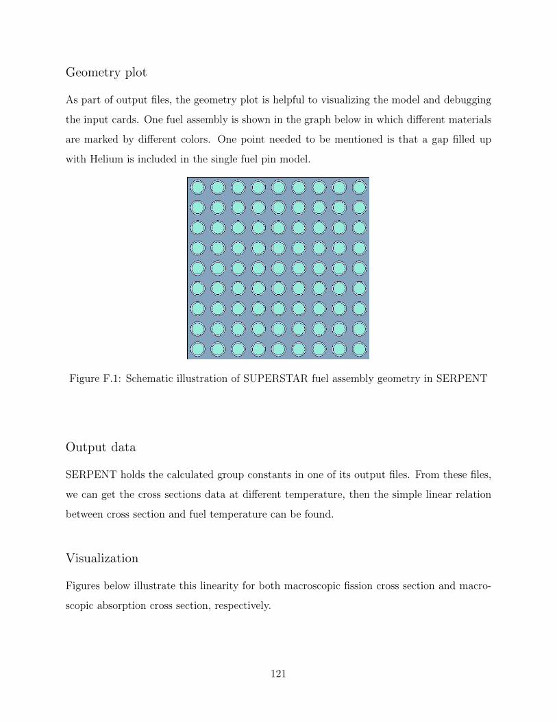
Geometry plot

As part of output files, the geometry plot is helpful to visualizing the model and debugging

the input cards. One fuel assembly is shown in the graph below in which different materials

are marked by different colors. One point needed to be mentioned is that a gap filled up

with Helium is included in the single fuel pin model.

Figure F.1: Schematic illustration of SUPERSTAR fuel assembly geometry in SERPENT

Output data

SERPENT holds the calculated group constants in one of its output files. From these files,

we can get the cross sections data at different temperature, then the simple linear relation

between cross section and fuel temperature can be found.

Visualization

Figures below illustrate this linearity for both macroscopic fission cross section and macro-

scopic absorption cross section, respectively.

121

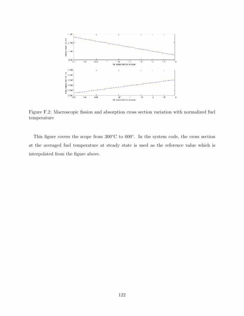
Figure F.2: Macroscopic fission and absorption cross section variation with normalized fueltemperature

This figure covers the scope from 300◦C to 600◦. In the system code, the cross section

at the averaged fuel temperature at steady state is used as the reference value which is

interpolated from the figure above.

122

REFERENCES

[1] James Sienicki, Sara Bortot, Anton Moisseytsev, Qiyue Lu, and Gerardo Aliberti, StatusReport on LFR Demonstartor Development, ANL-FCRD-135, Nov 29 2010.

[2] James Sienicki, Sara Bortot, Anton Moisseytsev, Qiyue Lu, and Gerardo Aliberti, SU-PERSTAR: An Improved Natural Circulation, Lead-Cooled, Small Modular Fast Reactorfor International Deployment, Proceedings of ICAPP 2011, Nice, France, May 2011.

[3] S. Bortot, A. Moisseytsev, J.J. Sienicki and Carlo Artioli, Core design investigation for aSUPERSTAR small modular lead-cooled fast reactor demonstrator, Nuclear Engineeringand Design, 241, 3021-3031, 2011.

[4] Alessandro Alemberti, Johan Carlsson, Edouard Malambu, Alfredo Orden, DankwardStruwe, Pietro Agostini and Stefano Monti, European lead fast reactor-ELSY, NuclearEngineering and Design, 241 3470-3480, 2011.

[5] Sara Bortot, Patrizio Console Camprini, Giacomo Grasso and Carlo Artioli, ConceptualCore Design Study for a High-flux LFR Demonstrator, Progress in Nuclear Energy,Volume 54, Issue 1, 56-63, Jan 2012.

[6] Alessandro Alemberti, Valery Smirnov, Craig F. Smith and Minoru Takahashi, Overviewof lead-cooled fast reactor activities, Progress in Nuclear Energy, 2013.

[7] Alan E. Waltar and Albert B. Reynolds, Fast Breeder Reactors, Pergamon Press, 1981.

[8] J.March-Leuba and E.D.Blakeman, A Mechanism for Out-of-Phase Power Instabilitiesin Boiling Water Reactors, Nucl. Sci. Eng., v.107, 173, 1991.

[9] Atul A. Karve, Nuclear-Coupled Thermal-Hydraulic Stability Analysis of Boiling WaterReactor, Ph.D thesis, University of Virginia, Jan 1998.

[10] Quan Zhou, Stability and Bifurcation Analyses of Reduced-Order Models of Forced andNatural Circulation BWRs, Ph.D thesis, University of Illinois at Urbana-Champaign,2006.

[11] Quan Zhou, Rizwan-uddin, In-Phase and Out-of-Phase Oscillations in BWRs: Impactof Azimuthal Asymmetry and Second Pair of Eigenvalues, Nuc. Sci. Eng,151.95-113,2005.

123

[12] V. Dykin, C. Demazire, C. Lange and D. Hennig, Investigation of global and regionalBWR instabilities with a four heated-channel Reduced Order Model, Annals of NuclearEnergy, 53, 381-400, 2013.

[13] V. Dykin, C. Demazire, C. Lange and D. Hennig, Investigation of local BWR instabilitieswith a four heated-channel Reduced Order Model, Annals of Nuclear Energy, 53, 320-330,2013.

[14] R.T.Lahey and F.J.Moody, The Thermal-Hydraulics of a Boiling Water Nuclear Reac-tor, 2nd edition, American Nuclear Society, La Grange Park, Illinois, 1993.

[15] D.S. Pilkhwal, W. Ambrosini, N. Forgione, P.K. Vijayan, D. Saha, J.C. Ferreri, Anal-ysis of the Unstable Behaviour of a Single-Phase Natural Circulation Loop with One-dimensional and Computational Fluid-Dynamic Models, Annals of Nuclear Energy, 34,339-355, 2007.

[16] K. Nagy, D. Lathouwers, C.G.A TJoen, J.L. Kloosterman and T.H.J.J. van der Hagen,Steady-state and Dynamic Behavior of a Moderated Molten Salt Reactor, Annals ofNuclear Energy, 2013.

[17] C.T.Joen and M.Rohde, Experimental Study of the Coupled Thermal-Hydraulic-Neutronic Stability of a Natural Circulation HPLWR, Nuclear Engieering and Design,Volume 242, 221-232, Jan 2012.

[18] Prashant Kumar Jain, Numerical Analysis of Supercritical Flow Instability In A NaturalCirculation Loop, Master Thesis, University of Illinois at Urbana-Champaign, 2006.

[19] Weston M. Stacey, Space-time Nuclear Reactor Kinetics, Academic Press, Inc., 1969.

[20] Weston M. Stacey, Nuclear Reactor Physics, John Wiley & Sons, INC., 2001.

[21] Ziya Akcasu, Gerald S. Lellouche and Louis M. Shotkin, Mathematical Methods inNuclear Reactor Dynamics, Academic Press, 1971.

[22] Zuqia Huang, Fundamentals of Nuclear Reactor Kinetics, Peking University Press, 2007.

[23] Serpent-A Continuous-Energy Monte Carlo Reactor Physics Burnup Calculation Code,Users Manual, VTT Technical Research Centre, Finland, Aug, 2012.

[24] J.J.Duderstadt and L.J.Hamilton, Nuclear Reactor Analysis, New York:John Wiley &Sons, Inc., 1976.

[25] Sara Bortot, A.Cammi and Carlo Artioli, Dynamic Performance Assessment of MOXand Metallic Fuel Core Options for a Gen-IV LFR Demonstrator, Progress in NuclearEnergy, Volume 54, Issue 1, 112-122, Jan 2012.

[26] Jon Carmack, Steven L. Hayes and Douglas L. Porter, Fuels for Fast Spectrum Reactors,INL/MIS-10-18898, June, 2010

124

[27] L. Walters and D. Wade, An Innovative Particulate Metallic Fuel for Next GenerationNuclear Energy, Proceedings of ICAPP ’10, June 2010

[28] David Southall, Renaud Le Pierres, and Stephen J. Dewson, Design Considerations forCompact Heat Exchangers, Proceedings of ICAPP 08, Paper 8009, Anaheim, CA USA,June 8-12, 2008.

[29] Handbook on Lead-bismuth Eutectic Alloy and Lead Properties, Materials Compatibility,Thermal-hydraulics and Technologies 2007 Edition, OECD NEA No. 6195, ISBN 978-92-64-99002-9.

[30] P. Kundu, and I. Cohen, Fluid Mechanics, 4th Edition, Academic Press, 2008.

[31] N. E. Todreas and M. S. Kazimi, Nuclear System, Volume 1, 2nd Edition, Tay-lor&Francis, 2012.

[32] M. Necati Ozisik, Heat transfer: A Basic Approach, McGraw-Hill, 1985.

[33] John H. Lienhard IV and John H. Lienhard V, A Heat Transfer Textbook, PhlogistonPress, 3rd edition, 2005.

[34] Joseph Michael Doster, March 2013. Natural Circulation Systems,http://www4.ncsu.edu/∼doster/NE402/Text/SinglePhaseFlow/Partc.pdf

[35] B.T. Swapnalee and P.K. Vijayan, A Generalized Flow Equation for Single Phase Nat-ural Circulation Loops Obeying Mumtiple Friction Laws, International Journal of Heatand Mass Transfer, 54, 2011.

[36] J.Wang, W.X. Tian, Y.H. Tian, G.H. Su and S.Z. Qiu, A sub-channel analysis code foradvanced lead bismuth fast reactor, Progress in Nuclear Energy, 63, 34-48, 2013.

[37] Piyush Sabharwall, Effects of Fluid Axial Conduction on Liquid Metal Natural Circu-lation and Linear Stability, M.S thesis, Oregon State University, June 2004.

[38] Robert D. Cook, David S. Malkus, Michael E. Plesha and Robert J. Witt, Conceptsand Applications of Finite Element Analysis, 4th edition, Wiley, 2001.

[39] Sue Ann Campbell, Introduction to Delay Differential Equations, University of Water-loo, March 2007.

[40] Sun Leping, Stability Analysis for Linear Delay Differential Equations and NumericalExamples, Appl. Math.J.Chinese Univ.Ser.B, 18(4), 390-402, 2003.

[41] Tamas Kalmar-Nagy, Stability Analysis of Delay-differential Equations by the Method ofSteps and Inverse Laplace Transform, Differential Equations and Dynamical Systems,Vol. 17, 185-200, 2009.

[42] K. Engelborghs, T. Luzyanina and G. Samaey, DDE-BIFTOOL v. 2.00: a Matlabpackage for bifurcation analysis of delay differential equations, Users Manual, KatholiekeUniversiteit Leuven, Belgium, Oct, 2001.

125

[43] W. S. Yang, Fast Reactors Physics and Computational Methods, Nuclear engineeringand technoloty, Vol 44, No.2, March 2012.

126

Documents

c 2014 Qiyue Lu - IDEALS