c© 2016 by Rui Guo. All rights reserved.

ITEM PARAMETER DRIFT AND ONLINE CALIBRATION

BY

RUI GUO

DISSERTATION

Submitted in partial fulfillment of the requirementsfor the degree of Doctor of Philosophy in Psychology

in the Graduate College of theUniversity of Illinois at Urbana-Champaign, 2016

Urbana, Illinois

Doctoral Committee:

Professor Hua-Hua Chang, ChairAssistant Professor Steven Andrew CulpepperProfessor Jeffrey A. DouglasProfessor Lawrence J. HubertAssistant Professor Hans-Friedrich Kohn

Abstract

An important assumption of item response theory based computerized adaptive assessment is item parameter

invariance. Sometimes, however, item parameters are not invariant across different test administrations due

to factors other than sampling error; and this phenomenon is termed item parameter drift. Several methods

have been developed to detect drifted items, and most of the them were designed to detect drifts in the

unidimensional item response model under the paper and pencil testing framework, which may not be

adequate for computerized adaptive testing.

This paper introduces an online (re)calibration design to detect item parameter drift for computerized

adaptive testings in both unidimensional and multidimensional environment. Specifically, for online calibra-

tion optimal design in unidimensional computerized adaptive testing model, a modified two-stage design is

proposed by implementing a proportional density index algorithm. For a multidimensional computerized

adaptive testing model, a four-quadrant online calibration pretest item selection design with proportional

density index algorithm is proposed. Comparisons were made between different online calibration item

selection strategies. Results showed that under unidimensional computerized adaptive testing, the pro-

posed modified two-stage item selection criterion with proportional density algorithm outperformed the

other existing methods in terms of item parameter calibration and item parameter drift detection, and un-

der multidimensional computerized adaptive testing, the online (re)calibration technique with the proposed

four-quadrant item selection design with proportional density index outperformed other methods.

ii

To my parents, Shaopei Guo and Xinghua Liao, my husband, Shuo Tang, and my daughter, Renee Tang

iii

Acknowledgments

I would never have been able to finish my dissertation without the guidance of my committee members, help

from my friends, and support from my family and my husband.

I would like to express my deepest gratitude to my advisor, Dr. Hua-hua Chang, gratefully and sincerely,

for his excellent guidance, caring, understanding, patience, friendship, and providing me with an excellent

atmosphere for doing research during my graduate studies at the University of Illinois at Urbana-Champaign.

I am heartily thankful to him for his encouragement, guidance and passionate support from the initial to the

final, for letting me experience the research in the field and practical issues beyond the textbooks, patiently

corrected my writing and financially supported my research, for helping me develop my background in

statistics, psychometrics, quantitative educational psychology, and computer and web-based technology, and

for encouraging my research and for allowing me to grow as a research scientist. Dr. Chang has been

a tremendous mentor for me and his mentorship was paramount in providing a well rounded experience

consistent my long-term career goals, his advice on both research and my career priceless. He is not only

my academic and career mentor but also my life teacher.

I would also like to thank all of the members of department of quantitative psychology, educational

psychology and statistics, Dr. Steven Andrew Culpepper, Dr. Jeffrey A. Douglas, Dr. Lawrence J. Hubert,

Dr. Hans-Friedrich Kohn, who were willing to participate in my final defense committee at the last moment.

My research would not have been possible without their helps. Special thanks goes to Dr. Jeffrey A. Douglas,

who was always willing to help and give his best suggestions. I would also like to thank my fellow students,

who have helped me and supported me in any respect during the completion of my study. I also want to

thank you for letting my defense be an enjoyable moment, and for your brilliant comments and suggestions.

Lastly, I offer my regards and appreciation to my family, who has helped me through the process of

earning my graduate program. Words cannot express how grateful I am to my mother-in law, father-in-law,

my mother, and father for all of the sacrifices that you’ve made on my behalf. Your prayer for me was

what sustained me thus far. I would also like to thank all of my friends who supported me in writing, and

encouraged me to strive towards my goal. They were always supporting me and encouraging me with their

iv

best wishes. At the end I would like express appreciation to my beloved husband, Shuo Tang. He was always

there cheering me up and stood by me through the good times and bad.

v

Table of Contents

List of Tables . . . . . . . . . . . . . . . . . . . . . . . . . . . . . . . . . . . . . . . . . . . . . . viii

List of Figures . . . . . . . . . . . . . . . . . . . . . . . . . . . . . . . . . . . . . . . . . . . . . . ix

List of Abbreviations . . . . . . . . . . . . . . . . . . . . . . . . . . . . . . . . . . . . . . . . . x

Chapter 1 Introduction . . . . . . . . . . . . . . . . . . . . . . . . . . . . . . . . . . . . . . . 1

Chapter 2 Backgrounds . . . . . . . . . . . . . . . . . . . . . . . . . . . . . . . . . . . . . . . 62.1 Overview of Multidimensional Item Response Theory . . . . . . . . . . . . . . . . . . . . . . . 62.2 Overview of Computerized Adaptive Testing . . . . . . . . . . . . . . . . . . . . . . . . . . . . 92.3 Overview of Item Parameter Drift . . . . . . . . . . . . . . . . . . . . . . . . . . . . . . . . . 13

Chapter 3 Introduction to Online Calibration . . . . . . . . . . . . . . . . . . . . . . . . . . 153.1 Overview of Online Calibration . . . . . . . . . . . . . . . . . . . . . . . . . . . . . . . . . . . 153.2 Advantages of Online Calibration . . . . . . . . . . . . . . . . . . . . . . . . . . . . . . . . . . 163.3 Main Design Factors in Online Calibration . . . . . . . . . . . . . . . . . . . . . . . . . . . . . 173.4 Online Calibration as Applied Optimal Design . . . . . . . . . . . . . . . . . . . . . . . . . . 19

Chapter 4 Review of Existing Pretest Item Selection Methods . . . . . . . . . . . . . . . 214.1 Pretest Item Selection Methods in UCAT . . . . . . . . . . . . . . . . . . . . . . . . . . . . . 21

4.1.1 Random Selection . . . . . . . . . . . . . . . . . . . . . . . . . . . . . . . . . . . . . . 214.1.2 Examinee-Centered Adaptive Selection . . . . . . . . . . . . . . . . . . . . . . . . . . . 224.1.3 Item-Centered Selection . . . . . . . . . . . . . . . . . . . . . . . . . . . . . . . . . . . 22

4.2 Pretest Item Selection Method in MCAT . . . . . . . . . . . . . . . . . . . . . . . . . . . . . . 244.2.1 Random Selection . . . . . . . . . . . . . . . . . . . . . . . . . . . . . . . . . . . . . . 244.2.2 Examinee-Centered Selection . . . . . . . . . . . . . . . . . . . . . . . . . . . . . . . . 244.2.3 Item-Centered Selection and Optimal Design . . . . . . . . . . . . . . . . . . . . . . . 25

Chapter 5 Online Calibration Optimal Design Method . . . . . . . . . . . . . . . . . . . . 305.1 Four-Quadrant Optimal Design . . . . . . . . . . . . . . . . . . . . . . . . . . . . . . . . . . . 305.2 Optimal Design with Proportional Density Index Solution . . . . . . . . . . . . . . . . . . . . 36

5.2.1 The Proportional Density Index Algorithm . . . . . . . . . . . . . . . . . . . . . . . . 365.2.2 Online Calibration with PDI algorithm . . . . . . . . . . . . . . . . . . . . . . . . . . 42

5.3 Using Online (re)Calibration Design for IPD Detection . . . . . . . . . . . . . . . . . . . . . . 435.3.1 Using Sparse Matrix Calibration . . . . . . . . . . . . . . . . . . . . . . . . . . . . . . 435.3.2 Using Online Calibration to Detect IPD . . . . . . . . . . . . . . . . . . . . . . . . . . 44

vi

Chapter 6 Simulation Study . . . . . . . . . . . . . . . . . . . . . . . . . . . . . . . . . . . . 476.1 Simulation Designs . . . . . . . . . . . . . . . . . . . . . . . . . . . . . . . . . . . . . . . . . . 48

6.1.1 Study I: UCAT . . . . . . . . . . . . . . . . . . . . . . . . . . . . . . . . . . . . . . . . 486.1.2 Study II: MCAT . . . . . . . . . . . . . . . . . . . . . . . . . . . . . . . . . . . . . . . 50

6.2 Results . . . . . . . . . . . . . . . . . . . . . . . . . . . . . . . . . . . . . . . . . . . . . . . . . 526.2.1 Results of Study I . . . . . . . . . . . . . . . . . . . . . . . . . . . . . . . . . . . . . . 526.2.2 Results of Study II . . . . . . . . . . . . . . . . . . . . . . . . . . . . . . . . . . . . . . 606.2.3 Conclusions . . . . . . . . . . . . . . . . . . . . . . . . . . . . . . . . . . . . . . . . . . 61

Chapter 7 Discussion . . . . . . . . . . . . . . . . . . . . . . . . . . . . . . . . . . . . . . . . . 637.1 Conclusions . . . . . . . . . . . . . . . . . . . . . . . . . . . . . . . . . . . . . . . . . . . . . . 637.2 Future Directions . . . . . . . . . . . . . . . . . . . . . . . . . . . . . . . . . . . . . . . . . . . 64

Appendix A Information Matrix of Parameters in 2D2PL Model . . . . . . . . . . . . . . 67

References . . . . . . . . . . . . . . . . . . . . . . . . . . . . . . . . . . . . . . . . . . . . . . . . 69

vii

List of Tables

4.1 Values of µ∗ and w∗ for selected b for 4−point designs. Reprinted from “D-optimal designsfor logistic regression in two variables”, Haines, Linda M and Kabera, Gaetan and O’Brien,Timothy E . . . . . . . . . . . . . . . . . . . . . . . . . . . . . . . . . . . . . . . . . . . . . . 29

viii

List of Figures

2.1 Surface Plot of A M2PL Model with a1 = 1.2, a2 = .7 and b = 0 . . . . . . . . . . . . . . . . 82.2 Contour Plot of A M2PL Model with a1 = 1.2, a2 = .7 and b = 0 . . . . . . . . . . . . . . . 8

4.1 A two-dimensional design space with four optimal design points . . . . . . . . . . . . . . . . . 274.2 A two-dimensional design space with out-of-boundary design points . . . . . . . . . . . . . . . 284.3 Haines et al.’s D-Optimal Design . . . . . . . . . . . . . . . . . . . . . . . . . . . . . . . . . . 29

5.1 A four-quadrant four-point design. . . . . . . . . . . . . . . . . . . . . . . . . . . . . . . . . . 325.2 A four-quadrant D-optimal design with symmetric conditions . . . . . . . . . . . . . . . . . . 335.3 PDI algorithm for a unidimensional IRT model . . . . . . . . . . . . . . . . . . . . . . . . . . 375.4 PDI algorithm for a two-dimensional IRT model . . . . . . . . . . . . . . . . . . . . . . . . . 385.5 Area Over A Region with Normal Distribution . . . . . . . . . . . . . . . . . . . . . . . . . . 405.6 A Multivariate Normal Distribution with Two Dimensions . . . . . . . . . . . . . . . . . . . . 415.7 Volume Over A Circle with Multivariate Normal Distribution . . . . . . . . . . . . . . . . . . 425.8 Using Online (re)Calibration for IPD Detection . . . . . . . . . . . . . . . . . . . . . . . . . . 44

6.1 Online (re)Calibration Design for IPD Detection . . . . . . . . . . . . . . . . . . . . . . . . . 476.2 BIAS and RMSE of a−parameter estimates in 2PL model . . . . . . . . . . . . . . . . . . . . 526.3 BIAS and RMSE of b−parameter estimates in 2PL model . . . . . . . . . . . . . . . . . . . . 536.4 BIAS and RMSE of a−parameter estimates in 3PL model . . . . . . . . . . . . . . . . . . . . 536.5 BIAS and RMSE of b−parameter estimates in 3PL model . . . . . . . . . . . . . . . . . . . . 546.6 BIAS and RMSE of c−parameter estimates in 3PL model . . . . . . . . . . . . . . . . . . . . 546.7 IPD detection in 2PL model . . . . . . . . . . . . . . . . . . . . . . . . . . . . . . . . . . . . . 556.8 IPD detection in 3PL model . . . . . . . . . . . . . . . . . . . . . . . . . . . . . . . . . . . . . 556.9 BIAS and RMSE of a1−parameter estimates in 2D2PL model . . . . . . . . . . . . . . . . . . 586.10 BIAS and RMSE of a2−parameter estimates in 2D2PL model . . . . . . . . . . . . . . . . . . 586.11 BIAS and RMSE of b−parameter estimates in 2D2PL model . . . . . . . . . . . . . . . . . . 596.12 IPD detection in 2D2PL model . . . . . . . . . . . . . . . . . . . . . . . . . . . . . . . . . . . 59

ix

List of Abbreviations

CAT Computerized adaptive testing

CD-CAT Cognitive diagnostic computerized adaptive testing

CDIF Compensatory differential item functioning

CMLE Conditional maximum likelihood estimation

CTT Classical test theory

DIF Differential item functioning

EAP Expected a-posteriori (estimation)

EM Expectation maximization (algorithm)

ESSA Every student succeed act

GRM Graded response model

ICC Item characteristic curve

IPD Item parameter drift

IRF Item response function

IRT Item response theory

JMLE Joint maximum likelihood estimation

LRT Likelihood ratio test

MAP Maximum a-posteriori (estimation)

MCAT Multidimensional computerized adaptive testing

MEM Marginal maximum likelihood estimate with multiple EM cycle

MIRT Multidimensional item response theory

MLE Maximum likelihood estimation

MLTM Multicomponent latent trait model

MMLE Marginal maximum likelihood estimation

M-MEM Multidimensional marginal maximum likelihood estimate with multiple EM cycle

M-Method A Multidimensional method A (algorithm)

x

M-OEM Multidimensional marginal maximum likelihood estimate with one EM cycle

M2PL Multidimensional two parameter logistic (model)

NCDIF Non-compensatory differential item functioning

OEM Marginal maximum likelihood estimate with one EM cycle

PDI Proportional density index (algorithm)

RMSE Root mean squared error

P & P Paper and pencil

RTTT Race to the top

SI Suitability index (algorithm)

Stepwise TCC Stepwise test characteristic curve

UCAT Unidimensional computerized adaptive testing

UIRT Unidimensional item response theory

1PL One parameter logistic (model)

2D2PL Two dimensional two parameter logistic (model)

2PL Two parameters logistic (model)

3PL Three parameters logistic (model)

xi

Chapter 1

Introduction

Linking and equating are important psychometric procedures that put test scores on the same scale so

that examinee performance is comparable across different test administrations. Since linking coefficients

are usually obtained from a set of common items used to anchor different administrations, the stability of

parameters of these common items is crucial to the quality of the linking process. Under item response

theory (IRT), any factor that may cause item parameter drift (IPD) across different administrations poses

a threat to the quality and validity of linking.

IPD can occur for various reasons, such as disclosure and sharing of items or social background change,

etc. The outcome of IPD includes, for example, in paper-and-pencil (P&P) testing, bad linking quality, score

incomparability; in computerized adaptive testing (CAT), bad θ estimation, inaccurate new items calibra-

tion and item bank contamination. Several methods have been developed to detect drifted items, including

non-IRT methods such as the Mantel-Haenszel method (Holland & Thayer, 1988) and IRT-based methods

such as the Lord’s chi-square statistic (Lord, 1980), the signed and unsigned areas between two item response

functions (Raju, 1990), the signed and unsigned closed-interval measures (kim1991comparison), the compen-

satory differential item functioning (CDIF) method, and the non-compensatory differential item functioning

(NCDIF) method (Raju, Van der Linden, & Fleer, 1995). While many of the above-mentioned methods are

based on comparing unidimensional IRT (UIRT) based item characteristic curves (ICCs) between adminis-

trations under P&P linear testings, R. Guo, Zheng, and Chang (2015) have used a stepwise test characteristic

curve (stepwise TCC) method that addresses the effects such as cancellation and amplification that previous

mentioned methods may have.

Furthermore, with the development of information technology, CAT has gained an increasing popularity

in many large scale high-stake educational testing programs in recent years. In fact, as president Obama has

signed the “Every Student Succeeds Act” (ESSA), CAT has been specifically mentioned and encouraged. A

CAT tailors the administered items sequentially according an examinee’s ability level as the test continues.

It successively selects test items whose difficulty level matches examinee’s current ability estimate given their

responses from previous test items, so that the precision of examinees’ final ability estimation is maximized

1

with a given test length. As a result, CAT can provide more accurate latent trait (θ) estimates using fewer

items than required by P&P tests (e.g., Weiss, 1982; Wainer & Mislevy, 1990).

One advantage of CAT is that it can provide uniformly precise scores for the majority of test-takers no

matter his/her ability is high, medium or low, and can show results immediately after the test like any

computer-based test. To the contrary, traditional linear testing always generate the highest estimation

precision for examinees with the medium ability levels, and increasingly poorer precision for test-takers with

more extreme test scores. In addition, CAT can shorten the test length by a half compared to a fixed length

P&P testing and still maintain a high level of precision than a fixed version. Therefore, test-takers save

more time in attempting items that are extremely hard or trivially easy. Test organizations also benefit

from substantially reduced cost from because of time savings and item development. Item exposure rate

is reduced as well because different examinees receive different sets of test items so that the test is more

secured.

However, the problem of IPD still exist in the framework of computerized adaptive testing. In fact,

the damage caused by IPD in CAT is even worse than in P&P, because IPD can directly affect students’

ability estimation, new items calibration, even the item pool. Existing ways of detecting IPD are the

same as in P&P. First, two sparse matrices need to be calibrated for two test administrations, followed

by a linking procedure, and then IPD detection methods such as Mantel-Haenszel, likelihood ratio testing,

etc., are performed. In a CAT program, nevertheless, it is hard to separate a continuous into two halves

naturally, and the response matrix generated is always sparse. With a sparse response matrix, not all of the

drifted items can be calibrated or recalibrated efficiently since some of the items may be answered by a very

small proportion of examinees. Furthermore, the calibration error in the process of recalibration could be

accumulated into the linking process, which further deteriorate the IPD detection quality.

With the federal grant program entitled “Race to the Top” (RTTT), schools are encouraged to develop

diagnostic tests (H.-h. Chang, 2012). With the diagnostic testing, students can be informed with diagnostic

information and teachers can make instructional decisions. Instead of providing a single test score, diagnostic

tests provide an ability profile on a given set of attributes/domains pertinent to learning and not simply a

global score or summative score of examinee’s ability. Therefore, in a large-scale achievement test, a single

subject may usually have multiple content domains. Several diagnostic psychometric models have been

proposed, including diagnostic classification models (e.g., Rupp, Templin, & Henson, 2012), multidimensional

item response theory (MIRT) models (e.g., Bolt & Lall, 2003; de la Torre & Patz, 2005; Embretson & Yang,

2013; S. J. Haberman & Sinharay, 2010; S. Haberman, Sinharay, & Puhan, 2009; Reckase, 1997, 2009;

Segall, 2001; S. J. Haberman & Sinharay, 2010) and etc., to provide psychometric foundations for diagnostic

2

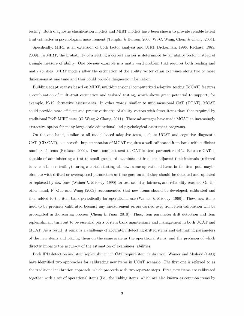
testing. Both diagnostic classification models and MIRT models have been shown to provide reliable latent

trait estimates in psychological measurement (Templin & Henson, 2006; W.-C. Wang, Chen, & Cheng, 2004).

Specifically, MIRT is an extension of both factor analysis and UIRT (Ackerman, 1996; Reckase, 1985,

2009). In MIRT, the probability of a getting a correct answer is determined by an ability vector instead of

a single measure of ability. One obvious example is a math word problem that requires both reading and

math abilities. MIRT models allow the estimation of the ability vector of an examinee along two or more

dimensions at one time and thus could provide diagnostic information.

Building adaptive tests based on MIRT, multidimensional computerized adaptive testing (MCAT) features

a combination of multi-trait estimation and tailored testing, which shows great potential to support, for

example, K-12, formative assessments. In other words, similar to unidimensional CAT (UCAT), MCAT

could provide more efficient and precise estimates of ability vectors with fewer items than that required by

traditional P&P MIRT tests (C. Wang & Chang, 2011). These advantages have made MCAT an increasingly

attractive option for many large-scale educational and psychological assessment programs.

On the one hand, similar to all model based adaptive tests, such as UCAT and cognitive diagnostic

CAT (CD-CAT), a successful implementation of MCAT requires a well calibrated item bank with sufficient

number of items (Reckase, 2009). One issue pertinent to CAT is item parameter drift. Because CAT is

capable of administering a test to small groups of examinees at frequent adjacent time intervals (referred

to as continuous testing) during a certain testing window, some operational items in the item pool maybe

obsolete with drifted or overexposed parameters as time goes on and they should be detected and updated

or replaced by new ones (Wainer & Mislevy, 1990) for test security, fairness, and reliability reasons. On the

other hand, F. Guo and Wang (2003) recommended that new items should be developed, calibrated and

then added to the item bank periodically for operational use (Wainer & Mislevy, 1990). These new items

need to be precisely calibrated because any measurement errors carried over from item calibration will be

propagated in the scoring process (Cheng & Yuan, 2010). Thus, item parameter drift detection and item

replenishment turn out to be essential parts of item bank maintenance and management in both UCAT and

MCAT. As a result, it remains a challenge of accurately detecting drifted items and estimating parameters

of the new items and placing them on the same scale as the operational items, and the precision of which

directly impacts the accuracy of the estimation of examinees’ abilities.

Both IPD detection and item replenishment in CAT require item calibration. Wainer and Mislevy (1990)

have identified two approaches for calibrating new items in UCAT scenario. The first one is referred to as

the traditional calibration approach, which proceeds with two separate steps. First, new items are calibrated

together with a set of operational items (i.e., the linking items, which are also known as common items by

3

convention), independently of the remaining operational items, and second, the resulting item parameters

are transformed to the scale of the operational items using linking methods, such as the Stocking-Lord

method (Stocking & Lord, 1983). Analogously, in IPD detection, two response matrices are usually calibrated

separately and linked.

Although it is possible to calibrate two separate response matrices for IPD detection, a more cost-effective

and commonly adopted approach is to embed the new items in operational tests. This approach is called

“online calibration”. Online calibration is referred to as dynamically select the pretest items for each

examinee during the operational test, update the parameter values, adjust the sampling process, until the

sampling process is finished.

In traditional CAT, online calibration method is commonly used to calibrate the new item parame-

ters (Ban, Hanson, Wang, Yi, & Harris, 2001; Chen, Xin, Wang, & Chang, 2012) on the fly. It has several

obvious advantages over the traditional approach, such as (1) all new items are placed on the same scale

as the operational items simultaneously so that no additional linking designs are required; (2) new items

can be seeded, most often randomly, in the test blindly so that examinees have the same motivation in

responding to the new items, and would give authentic responses to the new items; last but not least, (3)

item parameters of the new items and examinees’ unknown latent traits can be estimated jointly, which is

more cost-efficient (Chen et al., 2012). A foreseeable challenge with online calibration, which is related to

its design, is that only a subset of examinees answer each new item seeded in the operational test because

it is impossible for each examinee to answer all new items along with the operational items without fatigue

and other effects, resulting in typically sparse response matrix.

On the one hand, in the past several years, in order to overcome the data sparseness issue in CAT,

several online calibration methods have been developed and explored from both theoretical and practical

perspectives. For example, Stocking’s Method A and Method B (Stocking, 1988), marginal maximum likeli-

hood estimate with one EM cycle (OEM) method (Wainer & Mislevy, 1990), marginal maximum likelihood

estimate with multiple EM cycle (MEM) method (Ban et al., 2001), BILOG/Prior method (V. Folk &

Golub-Smith, 1996) and the marginal Bayesian estimation with Markov Chain Monte Carlo online calibra-

tion method (Segall, 2003). According to the inference in the presence of sparse matrix with systematic

missing data (Little & Rubin, 2002), researchers have verified the incorporation of marginal maximum like-

lihood estimation in to sparse data matrix (Mislevy & Wu, 1988), providing a theoretical foundation for

both OEM and MEM methods in online calibration. While all above mentioned methods were developed

under unidimensional IRT models, Chen, Zhang, and Xin (2013) successfully generalized three of them (i.e.,

Method A, OEM and MEM) to MCAT applications, denoted as M-Method A, M-OEM and M-MEM, re-

4

spectively, and found good item parameter recovery. More recently, on the other hand, an increasing number

of online calibration pretest item selection designs for UCAT have been developed, such as automatic online

calibration design (Makransky & Glas, 2014), sequential design (Y. c. I. Chang & Lu, 2010). However, few

pretest item selection designs have been proposed in the framework of MCAT. Thus, this article will explore

the possibility of finding a pretest item selection method in MCAT system.

Since IPD detection requires well recalibrated parameter values, it is natural to implement the technique

of online calibration into this process. Therefore, in the following section, an online (re)calibration pretest

item selection design will be introduced to detect item parameter drift for computerized adaptive testings in

both unidimensional and multidimensional environment. Specifically, under a UCAT scenario, a proportional

density index (PDI) algorithm will be introduced to modify a item selection criterion based on two-point

D-optimality design, while in MCAT a four-quadrant D-optimal solution implemented with PDI algorithm

will be proposed.

5

Chapter 2

Backgrounds

2.1 Overview of Multidimensional Item Response Theory

Classical test theory (CTT) and item response theory are two popular statistical frameworks for handling

test design and analysis. CTT had a longer history than IRT, while IRT is more statistical sophisticated.

The foundation of CTT is based on true score theory, and a total score is usually reported as the scoring

strategy Allen and Yen (2001). In CTT, the proportion of examinees who answer an item correctly is

regarded as the item difficulty level. Since examinee scores depend on the difficulty level of items and item

difficulty levels in turn depend on the ability levels of examinees, neither examinee ability estimates nor the

item difficulty levels are sample-invariant.

To the contrary, IRT uses a variation of the logistic regression models to represent the probability of

getting a correct answer. The probability depends on the examinee ability levels denoted as θ representing

the properties of examinees, and item parameters representing characteristics of items. The most commonly

used IRT models for dichotomous unidimensional scenario are the one-parameter logistic (1PL) model,

two-parameter logistic (2PL) model, and the three-parameter logistic (3PL) model. The probability of a

correct response to item j from examinee with ability level θ is modeled by the following item response

function (IRF):

Pj(θ) = cj +1− cj

1 + e−aj(θ−bj). (2.1)

In a 3PL model, aj , bj , cj represents discrimination, difficulty, and pseudo-guessing parameters, respectively.

The c−parameter allows that when examinee has no knowledge about solving the item but still can obtain

a correct answer by random guessing. When guessing is not allowed, a 2PL model is considered by setting

c = 0. Finally, when a 1PL model, or a Rasch model is considered, the discrimination (a−) parameter is

set to 1. The 1PL model has the strongest assumptions that all of the items administered having equal

discrimination power and no chance for guessing. The objective of item calibration is thus to estimate theses

6

item parameters using a series of statistical algorithms from a set of sampled response data.

The estimation of the item or examinee parameters relies on statistical algorithms. When item parameters

are known, or calibrated, examinee abilities are of interest. The most commonly used statistical estimation

methods for obtaining θ include maximum likelihood estimation (MLE), expected A-posteriori estimation

(EAP), and maximum A-posteriori estimation (MAP). When both examinee abilities and item parameters

are unknown and of interest, one may need to estimate θ’s and calibrate item parameters simultaneously.

One way of estimating both θ and (a−, b−, c−) parameters is to use the joint maximum likelihood estimation

(JMLE) algorithm. In 1PL model, this approach is successful, however, in more complicated models such

as 2PL and 3PL models, it becomes more difficult. A more sophisticated estimation routine is the marginal

maximum likelihood estimation (MMLE) with the expectation-maximization (EM) algorithm (MMLE-EM),

which first computes the posterior distribution of θ given responses data, and then maximize the expected

value of posterior likelihood by integrating out θ. Baker and Kim (2004) give a thorough presentation of the

variety of parameter estimation methods in IRT.

In many situations, an single test item may measure several latent traits rather than a single ability value.

One obvious example is a math word problem that requires both reading and math abilities. Within a single

content area, the content of an item is still able to measure multiple skills. For instance, an item about

the Pythagorean theorem may involve both algebra and geometry. This kind of items can be modeled by

MIRT, in which the probability of a getting correct response of an item is a function of a ability vector, θ,

rather than a single measure of ability, θ. MIRT models are more realistic than unidimensional IRT models

when a test item measures multiple traits. It can estimate an examinee’s algebra and geometry abilities

simultaneously by using one single test thus offer the potential to provide enhanced diagnostic information.

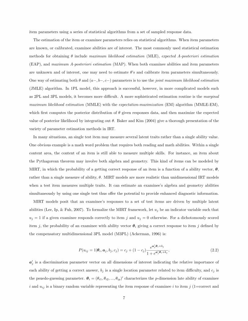
MIRT models posit that an examinee’s responses to a set of test items are driven by multiple latent

abilities (Lee, Ip, & Fuh, 2007). To formalize the MIRT framework, let uj be an indicator variable such that

uj = 1 if a given examinee responds correctly to item j and uj = 0 otherwise. For a dichotomously scored

item j, the probability of an examinee with ability vector θi giving a correct response to item j defined by

the compensatory multidimensional 3PL model (M3PL) (Ackerman, 1996) is:

P (uij = 1|θi,aj , bj , cj) = cj + (1− cj)ea′jθi+bj

1 + ea′jθi+bj

, (2.2)

a′j is a discrimination parameter vector on all dimensions of interest indicating the relative importance of

each ability of getting a correct answer, bj is a single location parameter related to item difficulty, and cj is

the psuedo-guessing parameter. θi = (θi1, θi2, ..., θip)′ characterizes the p-dimension late ability of examinee

i and uij is a binary random variable representing the item response of examinee i to item j (1=correct and

7

−2−1

01

2 −2

−1

0

1

2

0

0.2

0.4

0.6

0.8

1

θ1

θ2

Probability

Figure 2.1: Surface Plot of A M2PL Model with a1 = 1.2, a2 = .7 and b = 0

−2 −1.5 −1 −0.5 0 0.5 1 1.5 2−2

−1.5

−1

−0.5

0

0.5

1

1.5

2

θ1

θ 2

Figure 2.2: Contour Plot of A M2PL Model with a1 = 1.2, a2 = .7 and b = 0

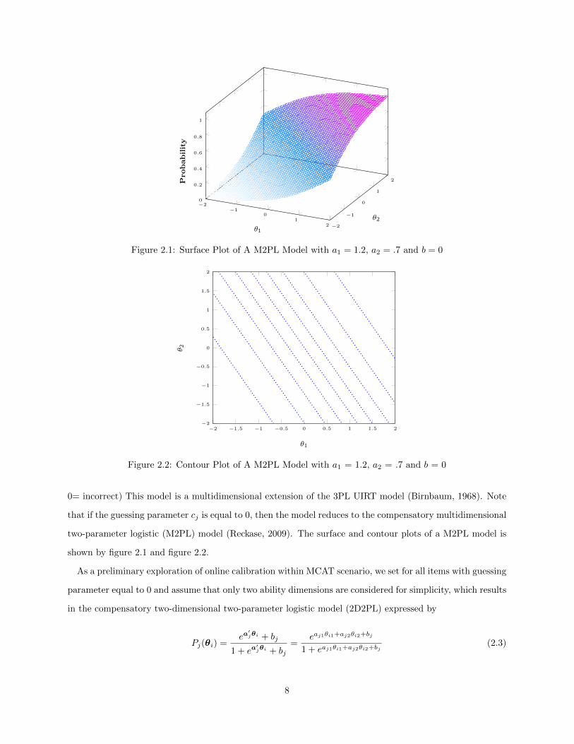
0= incorrect) This model is a multidimensional extension of the 3PL UIRT model (Birnbaum, 1968). Note

that if the guessing parameter cj is equal to 0, then the model reduces to the compensatory multidimensional

two-parameter logistic (M2PL) model (Reckase, 2009). The surface and contour plots of a M2PL model is

shown by figure 2.1 and figure 2.2.

As a preliminary exploration of online calibration within MCAT scenario, we set for all items with guessing

parameter equal to 0 and assume that only two ability dimensions are considered for simplicity, which results

in the compensatory two-dimensional two-parameter logistic model (2D2PL) expressed by

Pj(θi) =ea′jθi + bj

1 + ea′jθi + bj

=eaj1θi1+aj2θi2+bj

1 + eaj1θi1+aj2θi2+bj(2.3)

8

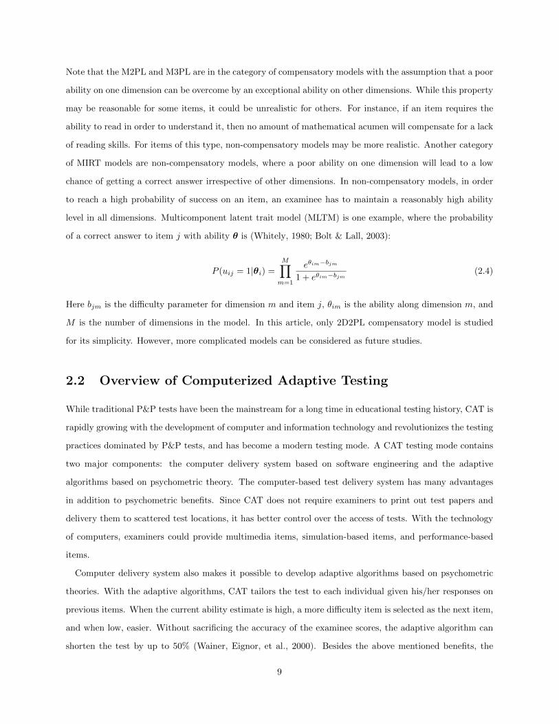
Note that the M2PL and M3PL are in the category of compensatory models with the assumption that a poor

ability on one dimension can be overcome by an exceptional ability on other dimensions. While this property

may be reasonable for some items, it could be unrealistic for others. For instance, if an item requires the

ability to read in order to understand it, then no amount of mathematical acumen will compensate for a lack

of reading skills. For items of this type, non-compensatory models may be more realistic. Another category

of MIRT models are non-compensatory models, where a poor ability on one dimension will lead to a low

chance of getting a correct answer irrespective of other dimensions. In non-compensatory models, in order

to reach a high probability of success on an item, an examinee has to maintain a reasonably high ability

level in all dimensions. Multicomponent latent trait model (MLTM) is one example, where the probability

of a correct answer to item j with ability θ is (Whitely, 1980; Bolt & Lall, 2003):

P (uij = 1|θi) =

M∏m=1

eθim−bjm

1 + eθim−bjm(2.4)

Here bjm is the difficulty parameter for dimension m and item j, θim is the ability along dimension m, and

M is the number of dimensions in the model. In this article, only 2D2PL compensatory model is studied

for its simplicity. However, more complicated models can be considered as future studies.

2.2 Overview of Computerized Adaptive Testing

While traditional P&P tests have been the mainstream for a long time in educational testing history, CAT is

rapidly growing with the development of computer and information technology and revolutionizes the testing

practices dominated by P&P tests, and has become a modern testing mode. A CAT testing mode contains

two major components: the computer delivery system based on software engineering and the adaptive

algorithms based on psychometric theory. The computer-based test delivery system has many advantages

in addition to psychometric benefits. Since CAT does not require examiners to print out test papers and

delivery them to scattered test locations, it has better control over the access of tests. With the technology

of computers, examiners could provide multimedia items, simulation-based items, and performance-based

items.

Computer delivery system also makes it possible to develop adaptive algorithms based on psychometric

theories. With the adaptive algorithms, CAT tailors the test to each individual given his/her responses on

previous items. When the current ability estimate is high, a more difficulty item is selected as the next item,

and when low, easier. Without sacrificing the accuracy of the examinee scores, the adaptive algorithm can

shorten the test by up to 50% (Wainer, Eignor, et al., 2000). Besides the above mentioned benefits, the

9

adaptive algorithms of CAT also allows continuous administration, where test takers can choose to take the

test at their preferred times and locations. If the traditional P&P testing mode is adopted, due to test security

and fairness concerns, the same test form cannot be used repeatedly during continuous administration, which

leads to an unreasonably high demand for test forms. In contrast, in CAT any examinee would receive a

unique set of items tailored to his/her performance on previous items.

Examples of CAT include the CAT version of the US Armed Service Vocational Aptitude Battery (CAT-

ASVAB), which is one of the most successful large-scale applications of CAT (Sands, Waters, & McBride,

1997). It was initiated in the 1970’s, developed in the 1980’s, launched in the 1990’s, and it continues to play a

critical role in US military personnel selection. Other famous large-scale CAT examples include the Graduate

Management Admission Test (GMAT), the National Council of State Boards of Nursing (NCSBN), and the

Graduate Record Examination (GRE). A typical computer-adaptive testing algorithm has the following

steps:

1. An optimal item is searched from the pool of available items based on the current estimate of the

examinee’s ability

2. The optimal item is administered to the current examinee, who then answers it either correctly or

incorrectly

3. Given a sequence of prior answers to the selected items, ability estimates are computed and updated

Steps 1-3 are repeated until a certain termination rule is satisfied and, as a result, different examinees

receive quite different tests. Furthermore, a CAT system typically consists of the following main components

according to Weiss and Kingsbury (1984):

1. A calibrated item pool from which items can be selected adaptively. A calibrated item pool is the

foundation of a CAT program. Operational items are selected from the item pool and administered to

the examinees sequentially. Items in the item pool should go through the pretest phase, which includes

the reliability and validity studies as well as item parameter calibration and equating.

2. The choice of the initial θ value, or a starting value of examinee’s ability. At the beginning of the test

when no prior information of the examinee ability is given, an initial θ value is needed. The θ value

can be initiated by using the mean value of the empirical distribution of the examinee ability or by

random sampling.

3. Item selection algorithm. The item selection methods are the most important factor in the CAT

system. A good item selection algorithm may generate a high examinee ability estimation efficiency,

10

while satisfying various non-statistical constraints such as content balancing, item exposure control,

word count, and answer key balancing (Zheng, 2014).

4. Intermediate and final θ estimation methods, or scoring procedure. CAT provides an efficient way

of assessing examinee ability θ, and a variety of methods have been developed for this purpose. For

example, MLE. Mislevy and Chang (2000) and H.-h. Chang and Ying (2009) have provided theoretical

proofs to support the legitimacy of using traditional MLE to estimate θ in CAT.

5. Termination criterion. Finally, when and where to stop a CAT process has always been an issue in

CAT studies. The CAT process can be terminated when a fixed length of items have been administered

to an examinee (called fixed length CAT), or a pre-specified standard error of estimation is reached

(called variable length CAT).

The adaptive item selection in CAT mimics what a wise examiner would do: if the examinee’s response

to the current item is correct, the next item would be harder, and vice versa (Wainer, 2000). In this way,

examinee can focus more on the items whose difficulty levels match his/her ability without wasting too much

time on many redundant, non-informative items.

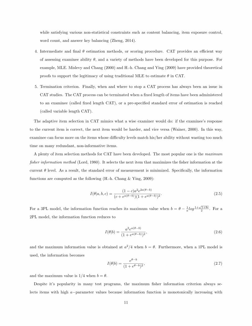
A plenty of item selection methods for CAT have been developed. The most popular one is the maximum

fisher information method (Lord, 1980). It selects the next item that maximizes the fisher information at the

current θ level. As a result, the standard error of measurement is minimized. Specifically, the information

functions are computed as the following (H.-h. Chang & Ying, 2009):

I(θ|a, b, c) =(1− c)a2e2a(θ−b)

(c+ ea(θ−b))(1 + ea(θ−b))2. (2.5)

For a 3PL model, the information function reaches its maximum value when b = θ − 1a log

1+√

1+8c2 . For a

2PL model, the information function reduces to

I(θ|b) =a2ea(θ−b)

(1 + ea(θ−b))2, (2.6)

and the maximum information value is obtained at a2/4 when b = θ. Furthermore, when a 1PL model is

used, the information becomes

I(θ|b) =eθ−b

(1 + eθ−b)2, (2.7)

and the maximum value is 1/4 when b = θ.

Despite it’s popularity in many test programs, the maximum fisher information criterion always se-

lects items with high a−parameter values because information function is monotonically increasing with

11

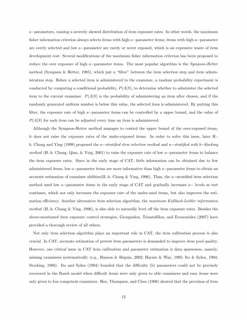
a−parameters, causing a severely skewed distribution of item exposure rates. In other words, the maximum

fisher information criterion always selects items with high a−parameter items; items with high a−parameter

are overly selected and low a−parameter are rarely or never exposed, which is an expensive waste of item

development cost. Several modifications of the maximum fisher information criterion has been proposed to

reduce the over exposure of high a−parameter items. The most popular algorithm is the Sympson-Hetter

method (Sympson & Hetter, 1985), which put a “filter” between the item selection step and item admin-

istration step. Before a selected item is administered to the examinee, a random probability experiment is

conducted by computing a conditional probability, P (A|S), to determine whether to administer the selected

item to the current examinee. P (A|S) is the probability of administering an item after chosen, and if the

randomly generated uniform number is below this value, the selected item is administered. By putting this

filter, the exposure rate of high a−parameter items can be controlled by a upper bound, and the value of

P (A|S) for each item can be adjusted every time an item is administered.

Although the Sympson-Hetter method manages to control the upper bound of the over-exposed items,

it does not raise the exposure rates of the under-exposed items. In order to solve this issue, later H.-

h. Chang and Ying (1999) proposed the a−stratified item selection method and a−stratified with b−blocking

method (H.-h. Chang, Qian, & Ying, 2001) to raise the exposure rate of low a−parameter items to balance

the item exposure rates. Since in the early stage of CAT, little information can be obtained due to few

administered items, low a−parameter items are more informative than high a−parameter items to obtain an

accurate estimation of examinee abilities(H.-h. Chang & Ying, 1996). Thus, the a−stratified item selection

method used low a−parameter items in the early stage of CAT and gradually increases a− levels as test

continues, which not only increases the exposure rate of the under-used items, but also improves the esti-

mation efficiency. Another alternative item selection algorithm, the maximum Kullback-Leibler information

method (H.-h. Chang & Ying, 1996), is also able to naturally level off the item exposure rates. Besides the

above-mentioned item exposure control strategies, Georgiadou, Triantafillou, and Economides (2007) have

provided a thorough review of all others.

Not only item selection algorithm plays an important role in CAT, the item calibration process is also

crucial. In CAT, accurate estimation of pretest item parameters is demanded to improve item pool quality.

However, one critical issue in CAT item calibration and parameter estimation is data sparseness, namely,

missing examinees systematically (e.g., Hanson & Beguin, 2002; Haynie & Way, 1995; Ito & Sykes, 1994;

Stocking, 1988). Ito and Sykes (1994) founded that the difficulty (b) parameters could not be precisely

recovered in the Rasch model when difficult items were only given to able examinees and easy items were

only given to less competent examinees. Hsu, Thompson, and Chen (1998) showed that the precision of item

12

recalibration can be affected by the sparseness response matrix of a CAT program.

Currently three approaches for item calibration are available. The first approach conducts a separate

“pretest” of the new items, calibrate their parameters, and link them to the existing scale. However, this

approach may lead to potential DIF due to different motivation and test environment, and it’s expensive.

The second approach embeds new items in operational tests, calibrate their parameters, and link them to

the existing scale. However, this approach might cause some test security issue because items are exposed to

every examinee. Also, in some settings, such as occupational testing, there is limited access to examinees for

calibration using the above two methods. Because of the limited access to examinees, it is always difficult

to collect adequate data to calibrate an item pool accurately. The third approach applies in on-the-fly

assembled tests, such as computerized adaptive tests, which dynamically select the pretest items for each

examinee during the operational test, update the parameter values, adjust the sampling, until the sampling

is finished. This approach is called “online calibration”.

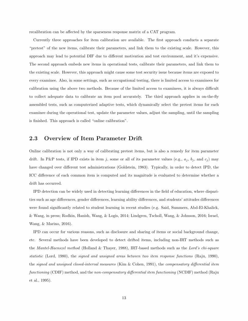
2.3 Overview of Item Parameter Drift

Online calibration is not only a way of calibrating pretest items, but is also a remedy for item parameter

drift. In P&P tests, if IPD exists in item j, some or all of its parameter values (e.g., aj , bj , and cj) may

have changed over different test administrations (Goldstein, 1983). Typically, in order to detect IPD, the

ICC difference of each common item is computed and its magnitude is evaluated to determine whether a

drift has occurred.

IPD detection can be widely used in detecting learning differences in the field of education, where dispari-

ties such as age differences, gender differences, learning ability differences, and students’ attitudes differences

were found significantly related to student learning in recent studies (e.g. Said, Summers, Abd-El-Khalick,

& Wang, in press; Rodkin, Hanish, Wang, & Logis, 2014; Lindgren, Tscholl, Wang, & Johnson, 2016; Israel,

Wang, & Marino, 2016).

IPD can occur for various reasons, such as disclosure and sharing of items or social background change,

etc. Several methods have been developed to detect drifted items, including non-IRT methods such as

the Mantel-Haenszel method (Holland & Thayer, 1988), IRT-based methods such as the Lord’s chi-square

statistic (Lord, 1980), the signed and unsigned areas between two item response functions (Raju, 1990),

the signed and unsigned closed-interval measures (Kim & Cohen, 1991), the compensatory differential item

functioning (CDIF) method, and the non-compensatory differential item functioning (NCDIF) method (Raju

et al., 1995).

13

On the one hand, many of the above-mentioned methods are based on comparing item characteristic curves

(ICCs) between administrations. The limitation of using ICC for IPD detection lies in the amplification

effect, which shows obvious IPD at the overall TCC level when the items drift towards the same direction,

and the cancellation effect, which means that when two sets of individual items drift towards opposite

directions, their IPD may cancel each other out at the overall test score level, leaving the TCC un-drifted.

One example of applicable settings of this effect is item response theory based true score equating, whose

goal is to generate a conversion table to relate number-correct scores on two test forms based on their test

characteristic curves (Kolen & Brennan, 2004). Since the conversion table is completely determined by TCCs

between administrations, the equating result is affected by TCCs only, instead of individual ICCs, and the

removal of a drifted item is unnecessary as long as the overall TCCs do not show drift.

R. Guo et al. (2015) presented a stepwise test characteristic curve method (referred to as the stepwise

TCC method), which iteratively searches for a collection of items that jointly causes TCC drift. Inspired by

the stepwise regression method (e.g., Cook & Weisberg, 2009) in statistics, which selects a locally optimal

combination of predictive variables in a regression model, the stepwise TCC method method iteratively

removes some items that potentially cause TCC drift from the linking item set while bringing some excluded

items back. The process iterates until a locally optimal set of linking items is found. The benefits of the

proposed method are multifold. First, the algorithm is iterative and terminates automatically. Second, the

proposed method is especially effective when used with true score equating, because true score equating

is implemented through relating the TCCs of two test forms (Kolen & Brennan, 2004) and the proposed

method is designed to generate an accurate TCC by nature.

On the other hand, the above-mentioned methods are designed for unidimensional IRT in P&P testing.

However, few studies have been done in terms IPD in computerized adaptive testing case. In fact, the

outcome of IPD in computerized adaptive testing is even worse: it directly contaminates the whole item

pool and affects the estimation accuracy of examinees’ abilities and new items calibration. In this paper, an

online calibration target point design is proposed, which selects the examinees adaptively that can locally

minimize the standard error of estimation.

14

Chapter 3

Introduction to Online Calibration

3.1 Overview of Online Calibration

The application of computer-based online testing applications has been increased to a large extent in the

past years in different testing environment. In CAT, as test continues, some items in the existing pool would

be overexposed and obsolete so that replenishing and maintaining a secure and active item pool is crucial.

After old items have been excluded from the item pool, new items will be added into the pool. To be added

into the pool, new items have to be calibrated and transformed on the same scale as existing items in the

pool. Five general steps are identified for item bank replenishment (Zheng, 2014):

1. Items needing to be replenished are identified and excluded from the pool;

2. New items are written, reviewed, revised and added into a pretest item bank;

3. Pretest items are selected an administered to examinees during the CAT process;

4. Pretest items are exported from the sampling stage when it satisfies a certain stopping criteria;

5. Newly calibrated items are analyzed, calibrated, equated and added to the operational item bank.

Step 1 prepare the pretest item bank by identifying the items needing replenished. Steps 2 and 3 writes and

reviews new items. Step 4 is the pretest item selection step. During the operational CAT, pretest items

are selected from the pretest item pool through a pre-specified item selection criterion and administered to

the current examinee. Step 5 is then conducted to update item parameters after the examinee has finished

his/her test or when a pretest item has reached a certain predetermined stopping rule. Examinees’ responses

to these pretest items are used to calibrate pretest item parameters. Steps 4 and 5 are repeated for every

new examinee. The sampling procedure for one pretest item is terminated once a satisfactory precision of

parameter estimates is obtained or a target sample size is achieved. Then, this pretest item is exported

from the pretest item bank and calibrated. Finally the calibrated item is reviewed and, if passed, put into

operational item bank for testing purpose.

15

An accurately calibrated item bank is essential for a valid CAT. Currently three approaches for item

calibration are available. The first approach conducts a separate “pretest” of the new items, calibrate their

parameters, and link them to the existing scale of the item pool. However, this approach may lead to potential

differential item functioning (DIF) due to different motivation and test environment, and it’s expensive. The

second approach embeds new items in operational tests, calibrate their parameters, and link them to the

existing scale. However, this approach might cause some test security issue because items are exposed to

every examinee. Also, in some settings, such as occupational testing, there is limited access to examinees

for calibration using the above-mentioned two methods. Because of the limited access to examinees, it is

always difficult to collect adequate data to calibrate an item pool accurately from an occupational setting.

The third approach uses online calibration, which dynamically select the pretest items for each examinee

during the operational test, update the parameter values, adjust the sampling, until the sampling procedure

is finished.

According to Kingsbury (2009), the general idea of online calibration takes advantage of the “transitivity

of examinee and item in item response theory to describe a process for adaptive item calibration”. In other

words, online calibration indicates that during the course CAT, a pretest item is assigned to examinees whose

ability levels matches the prior parameter information of that item. The prior information can be obtained

from a given field-test or from calibration results given existing sample.

3.2 Advantages of Online Calibration

Within restricted time and a limited number of examinees, a carefully designed sequential sampling in

online calibration could increase the calibration precision of item parameters (e.g., Berger, 1992; Buyske,

2005; Jones & Jin, 1994). In other words, a well designed online calibration procedure can achieve the same

calibration accuracy with fewer examinees than a non-adaptive test. What’s more, since different examinee

receive a different set of pretest items, adaptive online calibration is more secure than a non-adaptive test

where every examinee is assigned the same pretest items.

The advantage of online calibration also lies in the following facts. First, it reduces the impact of dif-

ference in motivation and concerns of representativeness coming from the administration of pretest items

to volunteers (Parshall, 1998), and therefore, no differential item functioning would be introduced due to

different motivation and test environment. Second, it utilizes the pretest data obtained during operational

testing, so that parameters of the new items are on the same scale as those of the existing items. Hence,

linking procedure is not needed. Moreover, since different pretest items receive different examinee samples,

16

online calibration has lower item exposure rate for each pretest item, and thus poses less test security risk

than other item calibration method. Last, in adaptive testing, sequential sampling design could be used to

adjust and terminate the sampling process dynamically, which improves the efficiency of calibration. The

techniques of online calibration can also be used to detect potentially drifted items and recalibrate them.

3.3 Main Design Factors in Online Calibration

According to Zheng (2014), there are four main design factors in an online calibration design:

1. Pretest item selection method: how to find the optimal examinees that can calibrate each pretest item

most efficiently. Pretest items should be assigned examinees whose ability levels match their parameter

values. The pretest item selection method is one of the most important factor in online calibration,

and is the focus of this study.

2. Seeding location: where in a test the pretest items are embedded. The pretest items can be located

early, middle, late in the test. A hybrid seeding location can be employed as well.

3. Estimation method: This factor answers the question that given the sparse response data matrix,

which statistical algorithm should be used to estimate the pretest item parameters. In a traditional

calibration, researchers and practitioners often use “fixed-parameter calibration” (e.g., S. Kim, 2006)

to estimate item parameters. In fixed-parameter calibration, only a small part of items are needed

to be calibrated and their scales are equated to the well-prepared items. The estimation problem in

online calibration is essentially the same with fixed-parameter calibration, in which the operational

item parameters are fixed and the pretest item parameters are calibrated.

Online pretest item calibration is complicated because response matrix obtained from CAT adminis-

tration is always sparse because each examinee takes a unique set of test items selected from the item

pool based on his/her ability level (B. G. Folk & Golub-Simith, 1996; Haynie & Way, 1995; Hsu et al.,

1998; Stocking, 1988). Therefore, there is a relatively smaller sample size available than linear testing

mode for each pretest item. This data feature makes the calibration process of pretest items more

difficult to implement.

Several studies have proposed online pretest item calibration methods (B. G. Folk & Golub-Simith,

1996; Levine & Williams, 1998; Samejima, 2000; Stocking, 1988; Wainer & Mislevy, 1990). Ban et al.

(2001) summarized give most popular methods, as listed in the following:

17

• The Stocking-A method (Stocking, 1988). This method first estimates examinee ability θ’s using

all the administered operational items and then it estimates pretest item parameters using condi-

tional maximum likelihood estimation (CMLE) conditional on the estimated θ values. Stocking-A

is the simplest method to implement but may have low estimation precision because it used

examinees’ estimated θ values as their true ones.

• The Stocking-B method (Stocking, 1988). This method is essentially Stocking-A method by

adding one more equating step.

• The marginal maximum likelihood estimation (MMLE) with one expectation-maximization (EM)

cycle method (OEM) method (Wainer & Mislevy, 1990). This method first computes the posterior

θ distribution of examinee ability from all of the operational items that have been already admin-

istered, which is further used to compute the marginal likelihood function in order to calibrate

item parameters.

• The MMLE with multiple EM cycles method (MEM) (Ban et al., 2001). This method is an

extension of the OEM method with its first cycle the exactly the same as OEM. From the second

cycle, both operational and pretest items are used to estimate the posterior θ distribution and to

calibrate pretest item parameters. The EM iteration is repeated until the parameter estimation

converges.

• The BILOG with Strong Prior method (Ban et al., 2001). This method utilizes the BILOG

(Mislevy & Bock, 1990) software to calibrate pretest items in one single run. The idea is to assign

some prior distributions on the operational items and then calibrate pretest and operational items

simultaneously.

In addition, by exploiting the Time-varying Markovian property of the examinee ability parameter, well

known recursive Bayesian estimators such as information filter, Kalman filter and extended Kalman

filter can be also considered as online calibration approaches(e.g. Li & Krolik, 2013b, 2012, 2011).

One major advantage of the above-mentioned online calibration methods is that the calibrated item

parameters are automatically on the same scale with the operational items. Therefore, no linking is

needed afterwards. This fact also explains the reason why online calibration can help detect item

parameter drift and recalibrate drifted items. For the MIRT model, Chen et al. (2013) has generalized

three of the above-mentioned methods, Stocking-A, OEM and MEM, from UCAT to MCAT, and the

corresponding names are M-Method A, M-OEM, and M-MEM. The following chapters will describe

these three methods in detail.

18

4. Termination rule: when to stop collecting samples of a pretest item and begin to estimate its value.

The sampling process can be stopped when a target sample size has been reached (e.g., Ali & Chang,

2011; Kingsbury, 2009), a satisfactory accuracy of item parameter estimation has been achieved, or

the item parameter estimates have been stabilized (Kingsbury, 2009).

5. Other factors: Other factors include the proportion of pretest items in a test, the minimum and

maximum sample size, etc.

3.4 Online Calibration as Applied Optimal Design

Online calibration pretest item selection is essentially an optimal design problem. In the design of exper-

iments, optimal design seeks to optimize some statistical criterion and allow parameters to be estimated

without bias and with minimum-variance. Optimal design has been used in many fields of study including

engineering, chemical engineering, education, biomedical and pharmaceutical research, business marketing,

epidemiology, medical research, environmental sciences, and manufacturing industry (Berger & Wong, 2005).

In the setting of educational testing, the application of optimal design includes two main aspects. One

is to select the optimal set of test items through algorithms such as maximum fisher information criterion

during operational CAT to maximize the accuracy of θ estimation, and the other is to assign an optimal

set of examinees to each pretest item through online calibration so that the precision of item calibration is

maximized. A natural and simple choice of item selection criterion in online calibration is random sampling,

which is useful when no prior information on examinee ability level is available. Random sampling is easy

to implement, can can provide a desirable calibration efficiency. Nevertheless, if the calibration sample is

chosen carefully to match pretest item parameter values, higher calibration efficiency can be obtained Berger

(1991). This sampling procedure can be achieved through “optimal sequential design” (Jones & Jin, 1994),

“sequential design” (Ying & Wu, 1997), or “sequential sampling design” (Berger, 1991).

In a 1PL UIRT model, one need to calibrate b−parameter only, and therefore, the sequential sampling

process only need to match examinees with b−parameters. In 2PL and 3PL UIRT models, the sampling

process need to not only match the properties of b−parameters, but also a− and/or c−parameters. As a

result, a compromise is often made to balance the needs of all parameters. Ying and Wu (1997) have shown

that sequential design converges to the optimal design under certain regularity conditions, and Y.-c. I. Chang

(2011) has proved the asymptotic consistency and efficiency of this design when covariates are subject to

errors.

Many procedures have been proposed under different scenarios to calibrate pretest items adaptively, or

19

sequentially, in UCAT. Examples include van der Linden and Glas (2000), Wainer, Dorans, Flaugher, Green,

and Mislevy (2000) and etc. Specifically, Jones and Jin (1994) and Y. c. I. Chang and Lu (2010) used

measurement error model method and D-optimal design to explore the sequential calibration design in a

2PL model. Kingsbury (2009) and Makransky and Glas (2014) explored the adaptive sequential design in

online calibration process also in a 2PL scenario. However, few literature have mentioned pretest item

selection method in MCAT so far. Sitter and Torsney (1995) have explored optimal designs for binary

response experiments with two design variables. However, the design space in their study is unlimited,

which is not the case for MIRT. Haines, Kabera, and O’Brien (2007) also investigated D-optimal designs for

logistic regression in two variables, but their design space is bounded by 0 and positive infinity for practical

reasons. Therefore, their optimal solutions might not fit the situation in MIRT, where θ vectors are usually

bounded by (−2, 2) because of standard normal distribution.

20

Chapter 4

Review of Existing Pretest ItemSelection Methods

This chapter provides a review of the current pretest item selection methods in online calibration for both

UCAT and MCAT models. The pretest item selection method studies how to match examinees with each

pretest item during the pretest stage, or how to assign examinees to each pretest item. Given limited sample

size and testing time, item calibration accuracy can be increased by optimal sequential sampling designs,

(e.g., Berger, 1991; Buyske, 2005; Jones & Jin, 1994), and this is the unique feature of online calibration.

In other words, compared with random sampling, which is often used in linear testing, an optimal sampling

design can be obtained by requiring fewer sample size to achieve the same calibration efficiency.

4.1 Pretest Item Selection Methods in UCAT

According to Zheng (2014), existing pretest item selection methods in UCAT can be summarized into three

categories: random selection, examinee-centered selection, and item-centered selection.

4.1.1 Random Selection

In random selection, a pretest item is randomly selected from the pretest item bank when an examinee

reaches seeding locations. In other words, each pretest item has equal opportunity to be chosen. Since

examinees ability distribution is normal, the selected examinees for a pretest item converges to a normal

distribution according to central limit theorem. Random selection method is easy to implement, ensures

equal sample size for every pretest item, and offers heterogeneous samples (e.g., Kingsbury, 2009; Chen et

al., 2012).

However, in an adaptive sequence, an item with a distinctively different difficulty level will stand out from

the surrounding when the difficulty of operational items generally follow a trend towards the examinees

ability level. Another issue is that when a student with low ability encounters a very difficult item, his or

her anxiety level may increase (Kingsbury, 2009). Also, as mentioned before, random selection is not the

most efficient way of sampling because higher calibration accuracy can be obtained through optimal design.

21

Therefore, another design recommended by Wainer and Mislevy (1990) and Ito and Sykes (1994) is that

both new and operational items can be administered to the examinees in an adaptive fashion and the

collected examinees’ responses to the new items are used to calibrate the new items.

4.1.2 Examinee-Centered Adaptive Selection

The second pretest item selection strategy is examinee-centered adaptive selection, in which pretest items are

selected using the same criterion as in operational CAT. When an examinee reaches seeding locations, item

selection criterion that maximize examinee estimation efficiency is used to select pretest items (Kingsbury,

2009; Chen et al., 2012). In particular, fisher information provides a measure of information of unknown

parameters from a sample of the population, and the inverse of the Fisher information yields the well known

Cramer Rao bounds on the variance of any unbiased estimators (Li & Krolik, 2015, 2014, 2013a).

As explained previously, the operational item selection criteria in CAT are aimed to optimize the esti-

mation efficiency of examinee abilities rather than to optimize the calibration efficiency of the pretest item

parameters. Therefore, this method aims at a different target. The examinee-centered adaptive selection

may be a reasonable choice for the 1PL model, since one only need to select examinees whose ability level

match b−parameters, but may not be appropriate for other IRT models where different item parameters

need different examinee ability locations (Zheng, 2014).

For example, in a 3PL model, the optimal examinees for calibrating c−parameters are the ones located

at the low end of the θ span, since c−parameters are the probability of getting a correct answer purely by

guessing. The optimal set of examinees for calibrating b−parameters are the ones located at the same place

at b−parameters, as shown in chapter 2. The optimal set of examinees for calibrating a−parameters are

generally located around the 20th and 80th quantile of the θ span. Hence, each parameter has a different

information curve and their peaks occur at different θ locations. Matching b−parameter with θ value only,

as operated in operational CAT procedure, will result in a high estimation efficiency for the b−parameter

and low precision for a− and c−parameters because little information is obtained at these locations.

4.1.3 Item-Centered Selection

The third strategy is the item-centered adaptive selection, which indicates that during the operational CAT,

at chosen seeding locations, pretest items are selected by criteria that are aimed to optimize the accuracy of

estimating pretest item parameters. Unlike examinee-centered selection, the item-centered strategy assigns

examinees to pretest items with a goal of optimizing estimation of the pretest item parameters instead of θ

values. Under UCAT model, several item-centered adaptive selection methods have been proposed, such as

22

Chang & Lu’s (2010) D-optimal design, Vander Linden & Ren’s (2014) D-optimal design, and Ali & Chang’s

suitability index design.

Chang & Lu’s D-Optimal Design One of the famous item-centered criterion in optimal calibration

design as well as in online calibration literature is the D-optimal criterion (Berger, 1992; Berger, King,

& Wong, 2000), which aims to find item parameter estimates that maximize the determinant value of the

fisher information matrix. The D-optimal criterion is commonly used in optimal designs (Silvey, 1980). One

example of using D-optimal to perform sequential sampling in online calibration is developed by Y. c. I. Chang

and Lu (2010), who divided the whole CAT process into two phases. The first phase is to conduct a normal

operational CAT to estimate examinee abilities, and the second phase is to conduct online calibration to

calibrate item parameters.

• Stage 1: Operational CAT is performed as a normal CAT process to estimate to estimate examinee

ability values.

• Stage 2: Pretest CAT is performed to select examinees using “2-point D-optimal criterion”. The “2-

point D-optimal criterion” finds two target points for each pretest item, and select examinees that are

close to the two target points. Specifically, the two target point, in a IRT model, are θ1 = −1.5434/a+b

and θ2 = 1.5434/a+ b.

Simulation studies have shown that selecting examinees located at the two target points only can optimize the

calibration efficiency of all parameters of a pretest item, making the two-stage design a desirable approach.

However, the two-stage design requires that all examinees form an “examinee pool” with known ability

values from which the optimal set of examinees can be chosen. In real practice, examinees come to the test

and leave after finishing, making the two-stage design hardly feasible.

Vander Linden & Ren’s D-optimal Design van der Linden and Ren (2014) proposed a D-optimal

design that can implemented in practice. In their design, each time at the seeding location D-optimal statistic

is computed for all pretest items and the one with the maximum value is selected. Besides its practical

possibility, this design tend to produce an unbalanced distribution of determinant values among pretest

items. Due to statistical reason, some items have always been able to provide higher determinant values

than others (Zheng, 2014). Therefore, this design is more prone to always select items whose determinant

values are higher than other items even if other items may need the current examinee more. With the

this D-optimal design, after the online calibration process finishes, some items may have high calibration

efficiency while others low. A natural improvement is to terminate the sampling process when a threshold

23

standard error of measurement is obtained or when a target sample size is reached, for example, Ren and

Diao (2013) imposed an exposure control in the item selection procedure to address the problem.

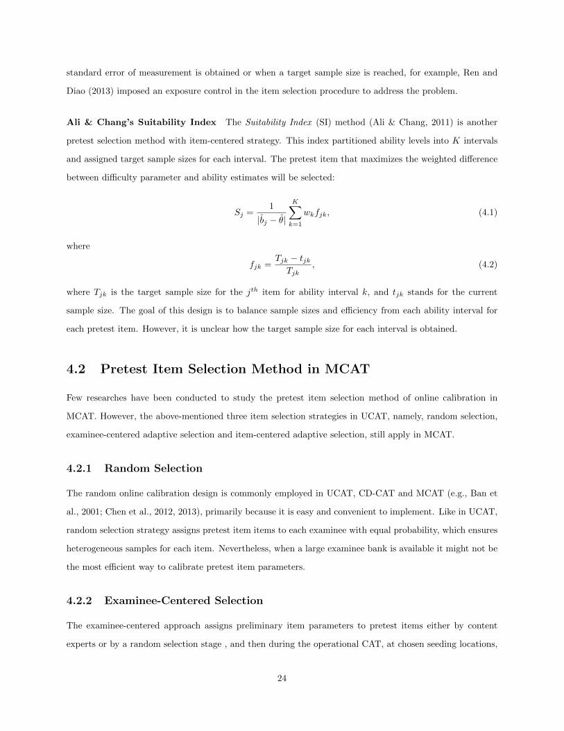
Ali & Chang’s Suitability Index The Suitability Index (SI) method (Ali & Chang, 2011) is another

pretest selection method with item-centered strategy. This index partitioned ability levels into K intervals

and assigned target sample sizes for each interval. The pretest item that maximizes the weighted difference

between difficulty parameter and ability estimates will be selected:

Sj =1

|bj − θ|

K∑k=1

wkfjk, (4.1)

where

fjk =Tjk − tjkTjk

, (4.2)

where Tjk is the target sample size for the jth item for ability interval k, and tjk stands for the current

sample size. The goal of this design is to balance sample sizes and efficiency from each ability interval for

each pretest item. However, it is unclear how the target sample size for each interval is obtained.

4.2 Pretest Item Selection Method in MCAT

Few researches have been conducted to study the pretest item selection method of online calibration in

MCAT. However, the above-mentioned three item selection strategies in UCAT, namely, random selection,

examinee-centered adaptive selection and item-centered adaptive selection, still apply in MCAT.

4.2.1 Random Selection

The random online calibration design is commonly employed in UCAT, CD-CAT and MCAT (e.g., Ban et

al., 2001; Chen et al., 2012, 2013), primarily because it is easy and convenient to implement. Like in UCAT,

random selection strategy assigns pretest item items to each examinee with equal probability, which ensures

heterogeneous samples for each item. Nevertheless, when a large examinee bank is available it might not be

the most efficient way to calibrate pretest item parameters.

4.2.2 Examinee-Centered Selection

The examinee-centered approach assigns preliminary item parameters to pretest items either by content

experts or by a random selection stage , and then during the operational CAT, at chosen seeding locations,

24

pretest items are selected by the same item selection method with the operational items.

In the case of MCAT, van der Linden (1999) proposed to select pretest items via a minimum error variance

criterion, while Veldkamp and van der Linden (2002) developed the Kullback-Leibler information criterion

originally proposed by H.-h. Chang and Ying (1996) in the UCAT case. Moreover, Mulder and van der

Linden (2009) introduced A-optimality (minimize the trace of the inverse of the information matrix) in

comparison to the traditional D-optimality (maximize the determinant of the information matrix). More

detailed research on can be found in Silvey (1980).

Despite the fact that the examinee-centered approach selects pretest items adaptively, it aims at a different

target because the selection strategy essentially maximizes the estimation examinee ability rather than

pretest items. Moreover, this approach generates uneven sample sizes for each item.

4.2.3 Item-Centered Selection and Optimal Design

Previous research on adaptive administrations of pretest items has focused on better scoring of test takers

instead of on improving calibration of the items themselves. To the contrary, item-centered adaptive selection

aims at the target of item calibration by focusing on accuracy of calibrated parameters, so that all pretest

items are equally taken care of. In UCAT, a lot of methods have been proposed to optimize the selection

procedure, as mentioned above; while in MCAT, few designs are found. For the optimal designs for logistic

model with two design variables, Sitter and Torsney (1995) and Haines et al. (2007) have provided some

guidance.

Sitter & Torsney’s D-Optimal Design Sitter and Torsney (1995) have studied the situation of two

design variables in a logistic regression model, as shown in the following:

p(θ) =ez

1 + ez, (4.3)

where z = b + a1θ1 + a2θ2. In the case of logistic regression with two predictors, they considered a design

boundary to prevent optimality criterion from being arbitrarily large. A bounded space is usually desirable

for practical reasons and can be made from particular interest.

Sitter and Torsney (1995) pointed out possible reasons why a bounded design space is desirable. First, a

moderate response probability would be more preferred since extreme values provide little information for

parameter estimation. This is always a consideration. Second, extremely high variable level is not desirable

for practical reasons. Therefore, it is obvious that these constraints can lead to different shapes of bounded

design regions in R2.

25

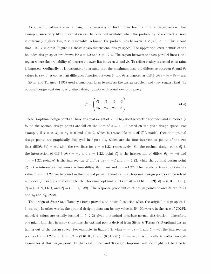
As a result, within a specific case, it is necessary to find proper bounds for the design region. For

example, since very little information can be obtained available when the probability of a correct answer

is extremely high or low, it is reasonable to bound the probabilities between .1 < p(z) < .9. This means

that −2.2 < z < 2.2. Figure 4.1 shows a two-dimensional design space. The upper and lower bounds of the

bounded design space are drawn for z = 2.2 and z = −2.2. The region between the two parallel lines is the

region where the probability of a correct answer lies between .1 and .9. To reflect reality, a second constraint

is imposed. Ordinarily, it is reasonable to assume that the maximum absolute difference between θ1 and θ2

values is, say, d. A convenient difference function between θ1 and θ2 is denoted as diff(θ1, θ2) = θ1−θ2 = ±d.

Sitter and Torsney (1995) used a canonical form to express the design problem and they suggest that the

optimal design contains four distinct design points with equal weight, namely:

ξ∗ =

d∗1 d∗2 d∗3 d∗4

.25 .25 .25 .25

(4.4)

These D-optimal design points all have an equal weight of .25. They used geometric approach and numerically

found the optimal design points are fall on the lines of z = ±1.22 based on the given design space. For

example, if b = 0, a1 = a2 = 0 and d = 2, which is reasonable in a 2D2PL model, then the optimal

design points are graphically displayed in figure 4.1, which are the four intersection points of the two

lines diff(θ1, θ2) = ±d with the two lines for z = ±1.22, respectively. So, the optimal design point d∗1 is

the intersection of diff(θ1, θ2) = +d and z = 1.22, point d∗2 is the intersection of diff(θ1, θ2) = +d and

z = −1.22, point d∗3 is the intersection of diff(x1, x2) = −d and z = 1.22, while the optimal design point

d∗4 is the intersection between the lines diff(θ1, θ2) = −d and z = −1.22. The details of how to obtain the

value of z = ±1.22 can be found in the original paper. Therefore, the D-optimal design points can be solved

numerically. For the above example, the D-optimal optimal points are d∗1 = (1.61,−0.39), d∗2 = (0.39,−1.61),

d∗3 = (−0.39, 1.61), and d∗4 = (−1.61, 0.39). The response probabilities at design points d∗1 and d∗3 are .7721

and d∗2 and d∗4, .2279.

The design of Sitter and Torsney (1995) provides an optimal solution when the original design space is

(−∞,∞). In other words, the optimal design points can be any value in R2. However, in the case of 2D2PL

model, θ values are usually located in (−2, 2) given a standard bivariate normal distribution. Therefore,

one might find that in many situations the optimal points derived from Sitter & Torsney’s D-optimal design

falling out of the design space. For example, in figure 4.2, when a1 = a2 = 1 and b = −2, the intersection

points of z = 1.22 and diff= ±2 is (2.61, 0.61) and (0.61, 2.61). However, it is difficulty to collect enough

examinees at this design point. In that case, Sitter and Torsney’ D-optimal method might not be able to

26

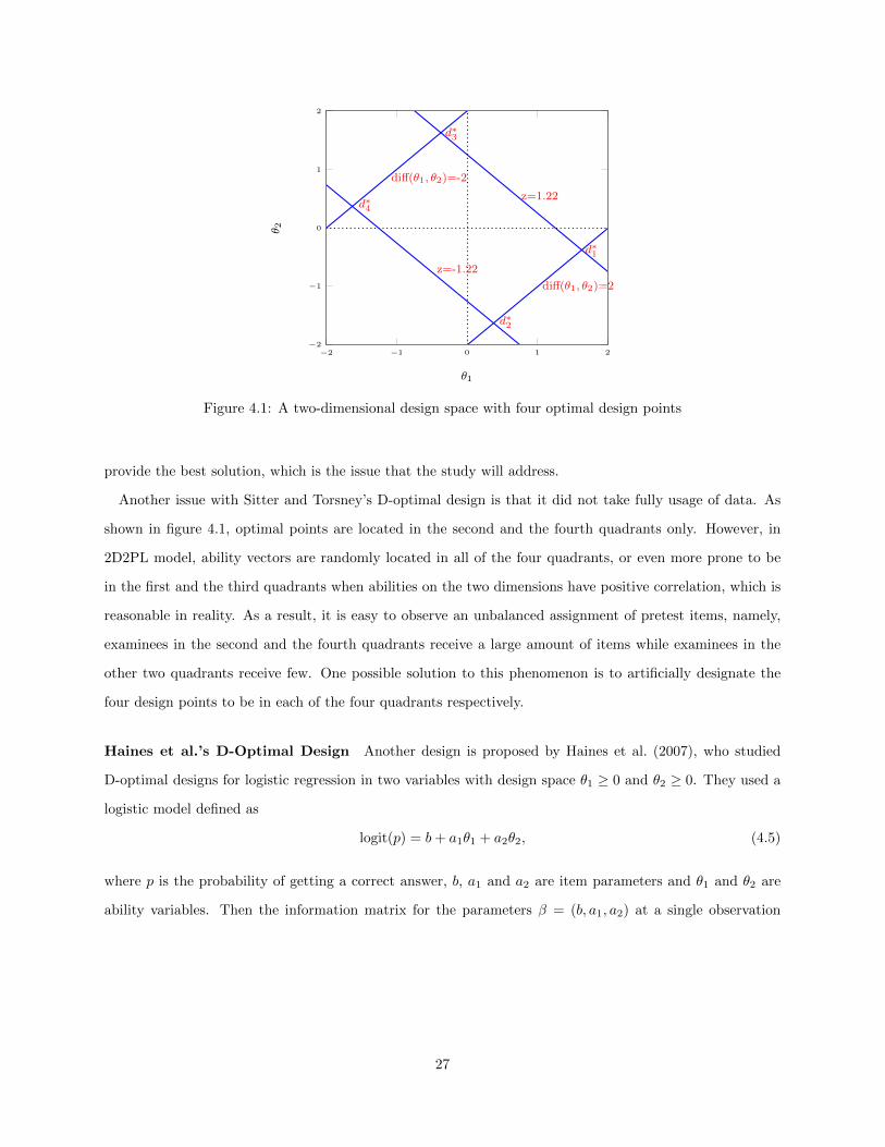
−2 −1 0 1 2−2

−1

0

1

2

d∗3

d∗2

d∗1

d∗4

diff(θ1, θ2)=-2

diff(θ1, θ2)=2

z=1.22

z=-1.22

θ1

θ 2

Figure 4.1: A two-dimensional design space with four optimal design points

provide the best solution, which is the issue that the study will address.

Another issue with Sitter and Torsney’s D-optimal design is that it did not take fully usage of data. As

shown in figure 4.1, optimal points are located in the second and the fourth quadrants only. However, in

2D2PL model, ability vectors are randomly located in all of the four quadrants, or even more prone to be

in the first and the third quadrants when abilities on the two dimensions have positive correlation, which is

reasonable in reality. As a result, it is easy to observe an unbalanced assignment of pretest items, namely,

examinees in the second and the fourth quadrants receive a large amount of items while examinees in the

other two quadrants receive few. One possible solution to this phenomenon is to artificially designate the

four design points to be in each of the four quadrants respectively.

Haines et al.’s D-Optimal Design Another design is proposed by Haines et al. (2007), who studied

D-optimal designs for logistic regression in two variables with design space θ1 ≥ 0 and θ2 ≥ 0. They used a

logistic model defined as

logit(p) = b+ a1θ1 + a2θ2, (4.5)

where p is the probability of getting a correct answer, b, a1 and a2 are item parameters and θ1 and θ2 are

ability variables. Then the information matrix for the parameters β = (b, a1, a2) at a single observation

27

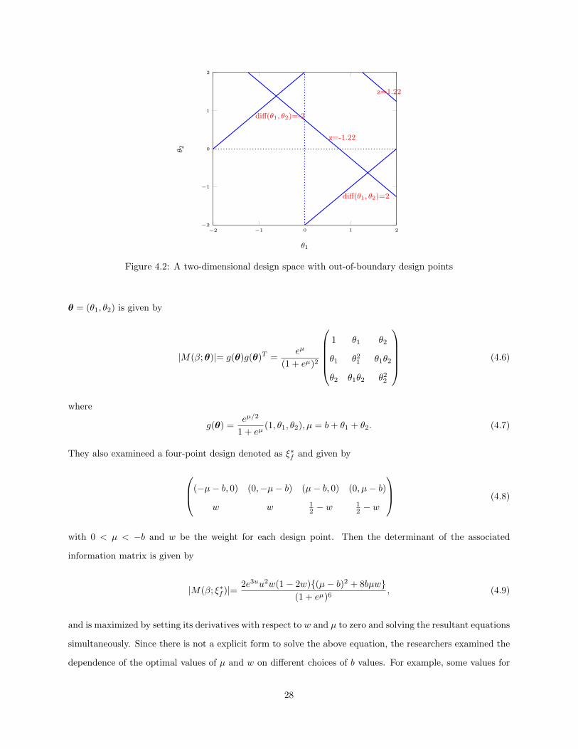
−2 −1 0 1 2−2

−1

0

1

2

diff(θ1, θ2)=-2

diff(θ1, θ2)=2

z=-1.22

z=1.22

θ1

θ 2

Figure 4.2: A two-dimensional design space with out-of-boundary design points

θ = (θ1, θ2) is given by

|M(β;θ)|= g(θ)g(θ)T =eµ

(1 + eµ)2

1 θ1 θ2

θ1 θ21 θ1θ2

θ2 θ1θ2 θ22

(4.6)

where

g(θ) =eµ/2

1 + eµ(1, θ1, θ2), µ = b+ θ1 + θ2. (4.7)

They also examineed a four-point design denoted as ξ∗f and given by

(−µ− b, 0) (0,−µ− b) (µ− b, 0) (0, µ− b)

w w 12 − w

12 − w

(4.8)

with 0 < µ < −b and w be the weight for each design point. Then the determinant of the associated

information matrix is given by

|M(β; ξ∗f )|= 2e3uu2w(1− 2w){(µ− b)2 + 8bµw}(1 + eµ)6

, (4.9)

and is maximized by setting its derivatives with respect to w and µ to zero and solving the resultant equations

simultaneously. Since there is not a explicit form to solve the above equation, the researchers examined the

dependence of the optimal values of µ and w on different choices of b values. For example, some values for

28

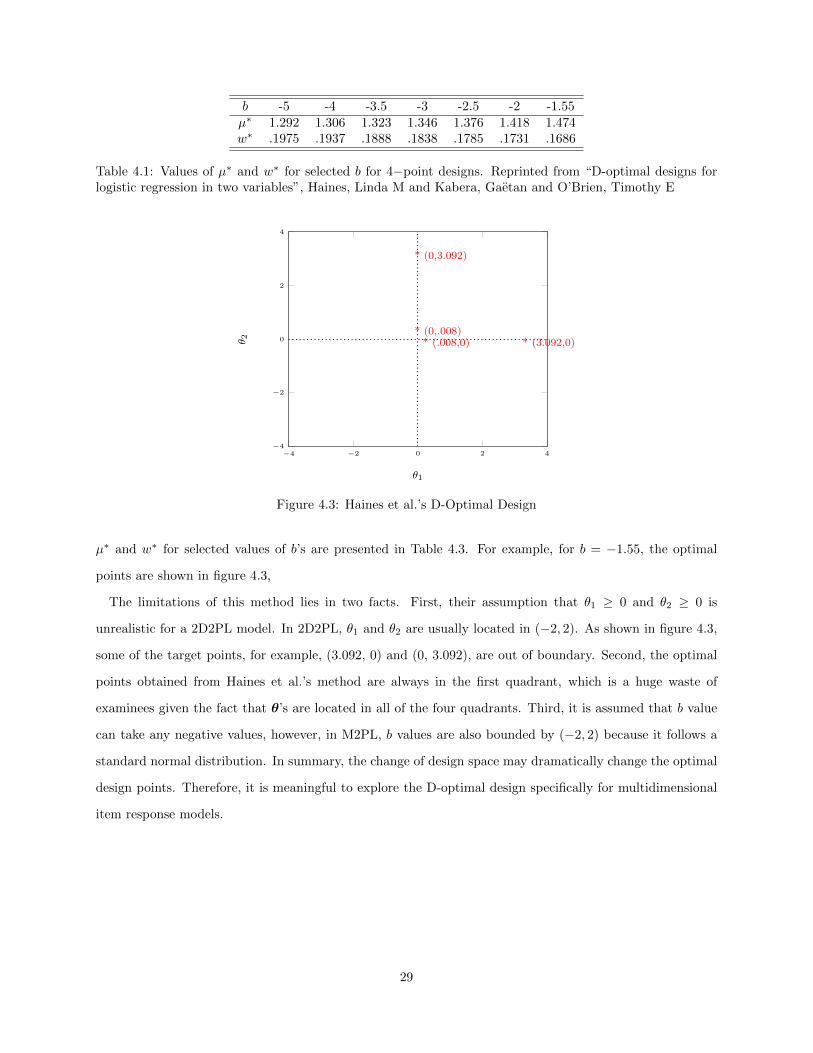
b -5 -4 -3.5 -3 -2.5 -2 -1.55µ∗ 1.292 1.306 1.323 1.346 1.376 1.418 1.474w∗ .1975 .1937 .1888 .1838 .1785 .1731 .1686

Table 4.1: Values of µ∗ and w∗ for selected b for 4−point designs. Reprinted from “D-optimal designs forlogistic regression in two variables”, Haines, Linda M and Kabera, Gaetan and O’Brien, Timothy E

−4 −2 0 2 4−4

−2

0

2

4

* (.008,0)* (0,.008)

* (3.092,0)

* (0,3.092)

θ1

θ 2

Figure 4.3: Haines et al.’s D-Optimal Design

µ∗ and w∗ for selected values of b’s are presented in Table 4.3. For example, for b = −1.55, the optimal

points are shown in figure 4.3,

The limitations of this method lies in two facts. First, their assumption that θ1 ≥ 0 and θ2 ≥ 0 is

unrealistic for a 2D2PL model. In 2D2PL, θ1 and θ2 are usually located in (−2, 2). As shown in figure 4.3,

some of the target points, for example, (3.092, 0) and (0, 3.092), are out of boundary. Second, the optimal

points obtained from Haines et al.’s method are always in the first quadrant, which is a huge waste of

examinees given the fact that θ’s are located in all of the four quadrants. Third, it is assumed that b value

can take any negative values, however, in M2PL, b values are also bounded by (−2, 2) because it follows a

standard normal distribution. In summary, the change of design space may dramatically change the optimal

design points. Therefore, it is meaningful to explore the D-optimal design specifically for multidimensional

item response models.

29

Chapter 5

Online Calibration Optimal DesignMethod

5.1 Four-Quadrant Optimal Design

In this chapter, a new pretest item selection online calibration design is introduced in a 2D2PL model. The

proposed design is item-centered, meaning that items are selected according to criteria based on matching

their properties. The proposed design is named four-quadrant D-optimal design. Specifically, optimal design

for maximum likelihood estimation of discrimination and location parameters of the 2D2PL model is con-

structed. The next sections are organized as follows: first, some properties of the 2D2PL model are discussed

along with techniques for its estimation. Then, the D-optimal criterion is defined and the corresponding

optimal design is derived.

The item response function of a 2D2PL model has the following form

P (θ) =ea1θ1+a2θ2+b

1 + ea1θ1+a2θ2+b, (5.1)

where θ = (θ1,θ2). P takes on values either 0 or 1. Letting the N observations in an experiment be

distinguished with the subscript i = 1, 2, ..., N , so that the observed probability under a 2D2PL model is

given by

P (θi) =ea1θi1+a2θi2+b

1 + ea1θi1+a2θi1+b, (5.2)

where θi = (θi1, θi2). Note that θi1 and θi2 are satisfying −2 < θi1 < 2 and −2 < θi2 < 2 since θi is following

a bivariate standard normal distribution. It can be shown that the information matrix of β = (a1, a2, b) for

an item for examinee i is

I(θi) =

Ia21(θi) Ia1a2(θi) Ia1b(θi)

Ia1a2(θi) Ia22(θi) Ia2b(θi)

Ia1a2(θi) Ia1b(θi) Ia22(θi)

= P (θi)Q(θi)

θ2i1 θi1θi2 θi1

θi1θi2 θ2i2 θi2

θi1 θi2 1

. (5.3)

30

Summing up N examinee,

I(θ) =

N∑i=1

P (θi)Q(θi)

θ2i1 θi1θi2 θi1

θi1θi2 θ2i2 θi2

θi1 θi2 1

, (5.4)

where Q(θi) = 1− P (θi).

In general, an optimal design is the one which maximize the information matrix I(θ). However, the

meaning of the word maximize, when applied to a matrix, is not obvious. Therefore, a number of criteria

have been proposed for maximization, such as D-optimality, A-optimality, E-optimality and etc. In this

article, only D-optimality is considered because it is one of the most popular criteria in optimal design

methodology for summarizing the information of multiple parameters (e.g., Berger, 1991, 1992; Berger et

al., 2000; Jones & Jin, 1994). Given ability values of all current available examinees, the D-optimal criterion

finds the item-parameter vector that maximizes the determinant of the fisher information matrix.

The criteria discussed above are applicable regardless of the number of levels θ of at which observations

are taken. Haines et al. (2007) examined both four-point and three-point designs for logistic regression with

two variables. However only four-point design with design region (−2, 2) will be considered in this article,

because 1) the four-point design is more commonly used (Sitter & Torsney, 1995; Haines et al., 2007); and

2) the three-point design is a special case of four-point design (Haines et al., 2007).

As mentioned before, the limitation of the Sitter & Torsney’s D-optimal design and Haines et al.’s D-

optimal design lie in two aspects primarily. One is that some of the optimal points might be out of the

design space, which means, their absolute values are larger than 97.5th or lower than 2.5th percentile of a

standard normal distribution. Few examinees are located at these locations, and therefore, it is hard to

collect enough sample size for calibration. The other limitation is that the optimal points always locate in

two quadrants only, which fails to take fully usage of the examinee data. Therefore, the proposed design

imposes a constraint that the four points must be in four quadrants respectively bounded by (-2, 2).

Let the four points be in four quadrants respectively in a two dimensional space, as shown in figure 5.1,

then using the aforementioned notation and restrictions, I(θ) can be reduced to

I(θ) =N

4

∑4k=1 θ

2k1P (θk)Q(θk)

∑4k=1 θk1θk2P (θk)Q(θk)

∑4k=1 θk1P (θk)Q(θk)∑4

k=1 θk1θk2P (θk)Q(θk)∑4k=1 θ

2k2P (θk)Q(θk)

∑4k=1 θk2P (θk)Q(θk)∑4

k=1 θk1P (θk)Q(θk)∑4k=1 θk2P (θk)Q(θk)

∑4k=1 P (θk)Q(θk)

, (5.5)

where k standards for the kth design point in the kth quadrant (k = 1, 2, 3, 4). The D-optimal criterion can

31

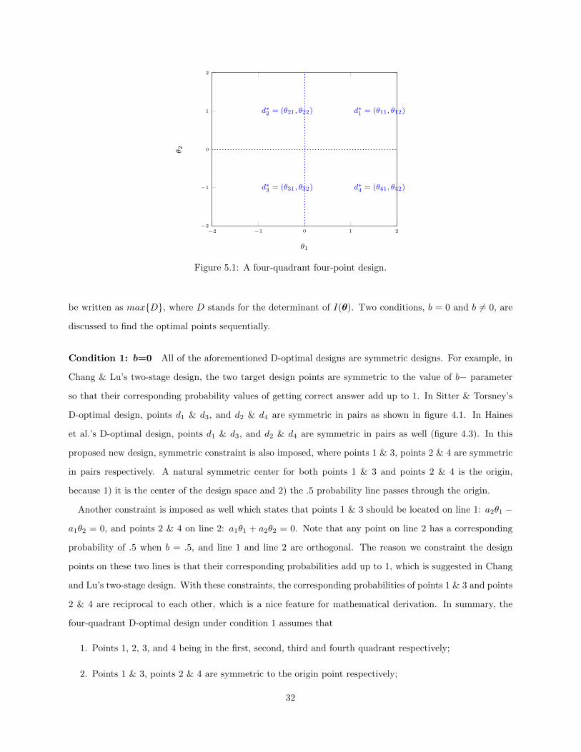
−2 −1 0 1 2−2

−1

0

1

2

d∗2 = (θ21, θ22)

d∗3 = (θ31, θ32)

d∗1 = (θ11, θ12)

d∗4 = (θ41, θ42)

θ1

θ 2

Figure 5.1: A four-quadrant four-point design.

be written as max{D}, where D stands for the determinant of I(θ). Two conditions, b = 0 and b 6= 0, are

discussed to find the optimal points sequentially.

Condition 1: b=0 All of the aforementioned D-optimal designs are symmetric designs. For example, in

Chang & Lu’s two-stage design, the two target design points are symmetric to the value of b− parameter

so that their corresponding probability values of getting correct answer add up to 1. In Sitter & Torsney’s

D-optimal design, points d1 & d3, and d2 & d4 are symmetric in pairs as shown in figure 4.1. In Haines

et al.’s D-optimal design, points d1 & d3, and d2 & d4 are symmetric in pairs as well (figure 4.3). In this

proposed new design, symmetric constraint is also imposed, where points 1 & 3, points 2 & 4 are symmetric

in pairs respectively. A natural symmetric center for both points 1 & 3 and points 2 & 4 is the origin,

because 1) it is the center of the design space and 2) the .5 probability line passes through the origin.

Another constraint is imposed as well which states that points 1 & 3 should be located on line 1: a2θ1 −

a1θ2 = 0, and points 2 & 4 on line 2: a1θ1 + a2θ2 = 0. Note that any point on line 2 has a corresponding

probability of .5 when b = .5, and line 1 and line 2 are orthogonal. The reason we constraint the design

points on these two lines is that their corresponding probabilities add up to 1, which is suggested in Chang

and Lu’s two-stage design. With these constraints, the corresponding probabilities of points 1 & 3 and points

2 & 4 are reciprocal to each other, which is a nice feature for mathematical derivation. In summary, the

four-quadrant D-optimal design under condition 1 assumes that

1. Points 1, 2, 3, and 4 being in the first, second, third and fourth quadrant respectively;

2. Points 1 & 3, points 2 & 4 are symmetric to the origin point respectively;

32

−2 −1 0 1 2−2

−1

0

1

2

d∗2

d∗3

d∗1

d∗4

line 1: a2θ1 − a1θ2 = 0

line 2: a1θ1 + a2θ2 = 0

θ1

θ 2

Figure 5.2: A four-quadrant D-optimal design with symmetric conditions

3. Points 1 & 3 are on line 1: a2θ1 − a1θ2 = 0; and

4. Points 2 & 4 are on line 2: a1θ1 + a2θ2 = 0.

Given the above constraints, the four-quadrant design can be shown in figure 5.2, and we can derive that

P1 = Q3, P3 = Q1

P2 = Q4 = P4 = Q2 = .5

and

θ31 = −θ11, θ32 = −θ12

θ41 = −θ21, θ42 = −θ22

, (5.6)

and the information matrix can be simplified to the following:

I(θ) =N

2

θ2

11P1Q1 + θ221P2Q2 θ11θ12P1Q1 + θ21θ22P2Q2 0

θ11θ12P1Q1 + θ21θ22P2Q2 θ212P1Q1 + θ2

22P2Q2 0

0 0 P1Q1 + P2Q2

, (5.7)

where P1 = P (θ1) and P2 = P (θ2). The determinant of the information matrix can be derived as

D =N

2P1Q1P2Q2(P1Q1 + P2Q2)(θ11θ22 − θ12θ21)2

=N

4P1Q1(P1Q1 + 1/4)(θ11θ22 − θ12θ21)2

(5.8)

Also since points 1 & 3 are on line 1, points 2 & 4 are on line 2, and the corresponding probability of point

33

1 is P1, we have a2θ11 − a1θ12 = 0

a1θ11 + a2θ12 = logit(P1)

a1θ21 + a2θ22 = 0

=⇒

θ11 = a1

a21+a22logit(P1)

θ12 = a2a21+a22

logit(P1)

θ22 = −a1a2 θ21

, (5.9)

where logit(P1) = ln P1

1−P1.The D value can be further simplified to

D =N

4[

a21

a2(a21 + a2

2)+

a1

a21 + a2

2

]2P1Q1(P1Q1 + 1/4)logit2(P1)θ221. (5.10)

Note that P1Q1(P1Q1 +1/4)logit2(P1) is independent of θ221, then maximizing D is equivalent to maximizing

P1Q1(P1Q1 + 1/4)logit2(P1) and θ221 simultaneously subject to the design space. Taking derivatives with

respect to P1 and set it equal to 0, the following can be obtained:

αD

αP1= C[logit2(P1)(4P 3

1 − 6P 21 +

3

2P1 +

1

4)+

2logit(P1)(1

P1+

1

1− P1)(P 4

1 − 2P 31 +

3

4P 2

1 +1

4P1)] = 0,

(5.11)

where C = N4 [

a21a2(a21+a22)

+ a1a21+a22

]2θ221. Solving Equation 5.11 the optimal solution for P (θ1) is 0.8838 and

the corresponding logit(P (θ1)) = 2.0286. Therefore, points 1 & 3 are

θ11 = 2.0286

a21+a22a1

θ12 = 2.0286a21+a22

a2

and

θ31 = − 2.0286

a21+a22a1

θ32 = − 2.0286a21+a22

a2

. (5.12)

For points 2 & 4, since θ221 is a concave function, the optimal θ21 is max{θ21} subject to θ21 ∈ (−2, 2) and

θ22 ∈ (−2, 2). Because θ22 = −a1a2 θ21, the constraints of θ21 and θ22 can be derived:

−2 < θ21 < 2

−2 < θ22 = −a1a2 θ21 < 2

=⇒ max{−2,−2a2

a1} < θ21 < min{2, 2a2

a1}, (5.13)

and −2 < θ22 < 2

−2 < θ21 = −a2a1 θ22 < 2

=⇒ max{−2,−2a1

a2} < θ22 < min{2, 2a1

a2}. (5.14)

34

If a1 ≥ a2, the above two equations reduce to

θ21 = −2a1a2

θ22 = 2

and

θ41 = 2a1a2

θ42 = −2

, (5.15)

otherwise if a1 < a2, θ21 = −2

θ22 = 2a2a1

and

θ41 = 2

θ42 = −2a2a1

. (5.16)

To summarize, the coordinates of the optimal four points are

Point 1: ( 2.0286a21+a22

a1,2.0286a21+a22

a2)

Point 2: (max{−2,−2a2a1 },min{2, 2a1a2 })

Point 3: (− 2.0286a21+a22

a1,− 2.0286a21+a22

a2)

Point 4: (min{2, 2a2a1 },max{−2,−2a1a2 })

Condition 2: b 6=0 In this condition, P1 and P3 no longer add up to 1 anymore because b 6= 0. However,

the four assumptions in condition 1 can still hold. It is easy to derive from the assumptions that

a1θ11 + a2θ12 + b = logitP1

a1θ31 + a2θ32 + b = logitP3

θ31 = −θ11, θ32 = −θ12

=⇒ P3 =e2b−logitP1

1 + e2b−logitP1(5.17)

Also since line 2 passes through the origin we have

a1(0) + a2(0) + b = logit(P2) =⇒

P2 = P4 = eb

1+eb

Q2 = Q4 = 11+eb

(5.18)

The information matrix becomes

I(θ) =N

4

θ211(P1Q1 + P3Q3) + 2θ221P2Q2 θ11θ12(P1Q1 + P3Q3) + 2θ21θ22P2Q2 0

θ11θ12(P1Q1 + P3Q3) θ212(P1Q1 + P3Q3) + 2θ222P2Q2 0

0 0 P1Q1 + P3Q3 + 2P2Q2

(5.19)

35

The determinant of I(θ) is then

D =N

4[(θ2

11(P1Q1 + P3Q3) + 2θ221P2Q2)(θ2

12(P1Q1 + P3Q3) + 2θ222P2Q2)

−(θ11θ12(P1Q1 + P3Q3) + 2θ21θ22P2Q2)2](P1Q1 + P3Q3 + 2P2Q2)

=N

2P2Q2(P1Q1 + P3Q3)(P1Q1 + P3Q3 + 2P2Q2)(θ11θ22 − θ12θ21)2

(5.20)

Substituting Equations 5.17 and 5.18, the determinant value becomes

D = C∗(P1Q1 +e2b−logitP1

(1 + e2b−logitP1)2)(P1Q1 +

e2b−logitP1

(1 + e2b−logitP1)2+

2eb

(1 + eb)2)logit2(P1)θ2

21, (5.21)

where C∗ is a constant. Although no closed form can be obtained for condition 2, a computer program is

helpful in finding the maximum determinant value through grid search. Assume the optimal P1 is denoted

as P ∗1 , then the target points are

Point 1: ( a1a21+a22

ln(P∗1

1−P∗1), a2a21+a22

ln(P∗1

1−P∗1))

Point 2: (max{−2,−2a2a1 },min{2, 2a1a2 })

Point 3: ( −a1a21+a22

ln(P∗1

1−P∗1), −a2a21+a22

ln(P∗1

1−P∗1))

Point 4: (min{2, 2a2a1 },max{−2,−2a1a2 })

5.2 Optimal Design with Proportional Density Index Solution

The four-quadrant four point optimal design is hardly feasible beyond simulation context because in an

operational CAT, examinees come to the test at varied times and leave afterwards. As a result, there is

hardly a static examinee pool to choose the optimal examinees from. In fact, the same situation holds for all

of the target points based optimal design (i.e., Chang & Lu’s two-stage design, Sitter & Torsney’s D-optimal

design, Haines et al.’s D-optimal design). In the following section, a practical online calibration algorithm,

the proportional density index algorithm, is introduced, which makes the four-quadrant D-optimal design

and other target point based designs applicable in real practice.

5.2.1 The Proportional Density Index Algorithm

The proportional density index (PDI) algorithm is a new framework for selecting pretest items adaptively.

The main idea of PDI algorithm is to set up a threshold boundary computed from the area for UIRT

model, or the volume of the circle centered at the target point for 2D2PL model. The distance between

36

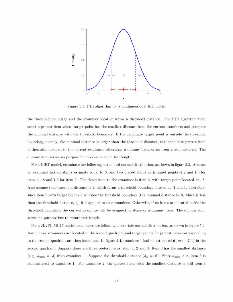
−3 −2 −1 0 1 2 3

0

0.1

0.2

0.3

0.4

*E*I1 *I2 *I1*I2

r r

x

Density

Figure 5.3: PDI algorithm for a unidimensional IRT model

the threshold boundary and the examinee location forms a threshold distance. The PDI algorithm then

select a pretest item whose target point has the smallest distance from the current examinee; and compare

the minimal distance with the threshold boundary. If the candidate target point is outside the threshold

boundary, namely, the minimal distance is larger than the threshold distance, this candidate pretest item

is then administered to the current examinee; otherwise, a dummy item, or no item is administered. The

dummy item serves no purpose but to ensure equal test length.

For a UIRT model, examinees are following a standard normal distribution, as shown in figure 5.3. Assume

an examinee has an ability estimate equal to 0, and two pretest items with target points -1.2 and 1.6 for

item 1, -.8 and 1.2 for item 2. The closet item to the examinee is item 2, with target point located at -.8.

Also assume that threshold distance is 1, which forms a threshold boundary located at -1 and 1. Therefore,

since item 2 with target point -.8 is inside the threshold boundary (the minimal distance is .8, which is less

than the threshold distance, 1), it is applied to that examinee. Otherwise, if no items are located inside the

threshold boundary, the current examinee will be assigned no items or a dummy item. The dummy item

serves no purpose but to ensure test length.

For a 2D2PL MIRT model, examinees are following a bivariate normal distribution, as shown in figure 5.4.

Assume two examinees are located in the second quadrant, and target points for pretest items corresponding

to the second quadrant are then found out. In figure 5.4, examinee 1 had an estimated θ1 = (−.7, 1) in the

second quadrant. Suppose there are three pretest items: item 1, 2 and 3. Item 3 has the smallest distance

(e.g., dmin = .3) from examinee 1. Suppose the threshold distance (dα = .6). Since dmin < r, item 3 is

administered to examinee 1. For examinee 2, the pretest item with the smallest distance is still item 3

37

−2 −1 0 1 2−2

−1

0

1

2

θ1

θ 2Threshold boundary circle

*I1*I2

*I3

*E1

*E2

Figure 5.4: PDI algorithm for a two-dimensional IRT model

(dmin = .8). Since dmin > r, no pretest items are assigned to examinee 2. To maintain the equal-length

test goal, a dummy item could be administered. To summarize, the following are the detailed steps of PDI

algorithm:

1. Specify which quadrant the current examinee falls into and find the target point for all the pretest

items in that quadrant;

2. Find the target points of each pretest item for the current examinee;

• In the unidimensional CAT, the target points are derived in section 4.1.3 proposed

by Y. c. I. Chang and Lu (2010). Suppose the coordinate of the target point is θ(t) for the

jth item.

• In the multidimensional CAT, first determine the quadrant the current examinee falls in, and then

find the corresponding target point for each pretest item. For example, if the current examinee

is in the first quadrant, then the target point for each pretest item is the one that resides in the

first quadrant as well. Suppose the coordinates of the target point is (θt1j , θt2j) for the jth item.

3. Compute the distance between the current examinee and the target point for each pretest item. Find

the pretest item with the smallest distance.

• In the unidimensional CAT case, for each examinee i with estimated ability θi, the distance is

computed by

dj = |θi − θ(t)j | (5.22)

38

• In the multidimensional CAT case, for each examinee i with estimated ability (θ1i, θ2i), compute

euclidean distances between examinee’s ability and the target point for each pretest item.

dj =

√(θ1i − θ(t)

1j )2 + (θ2i − θ(t)2j )2. (5.23)

If the smallest distance dmin is below the threshold distance (r), apply the pretest item; otherwise

apply a dummy item to the current examinee.

Threshold Distance r. Examinees are following a standard bivariate normal distribution, so that if

the target point of a pretest item is at the center point (0, 0), it is easier to reach the target sample size

because more examinees are available compared to a target point of (−2,−2), where few examinees are

located. For this reason, if the target point is close to the center point (0, 0), then the threshold distance

should be more stringent and the threshold boundary should be narrower, whereas if the target point

is far away from the center point, the threshold distance should be larger and the threshold boundary

should be broader. In detail, the threshold boundary is determined by

• Total number of examinees N . The higher the N , the smaller the threshold distance because

more examinees are available within a smaller area;

• Target sample size T . The higher the target sample size T , the larger the threshold distance,

because the demand for examinees is higher for each pretest items;

• Number of pretest items J . The higher the number of pretest items J , the larger the threshold

distance, because fewer examinees are allocated to each pretest item;

• Pretest length t. The higher the pretest length t, the smaller the threshold distance because

longer test length is equivalent to more examinees.

The idea of the threshold r for UCAT is to find the minimal distance such that the area inside the

threshold boundary is proportional to the available sample size. In MCAT, the threshold distance the

minimum radius for each target point such that the volume over the minimum circle is the same as

the available sample size. In UCAT, the threshold distance centered at the examinee location forms

a threshold boundary, while in MCAT, the circle centered at the target point with minimum radius

forms a boundary. Examinees inside the boundary are considered close enough to the target point,

which will be chosen as the calibration sample and the ones outside the boundary would be not used.

Therefore the threshold distance can be computed in the following way:

39

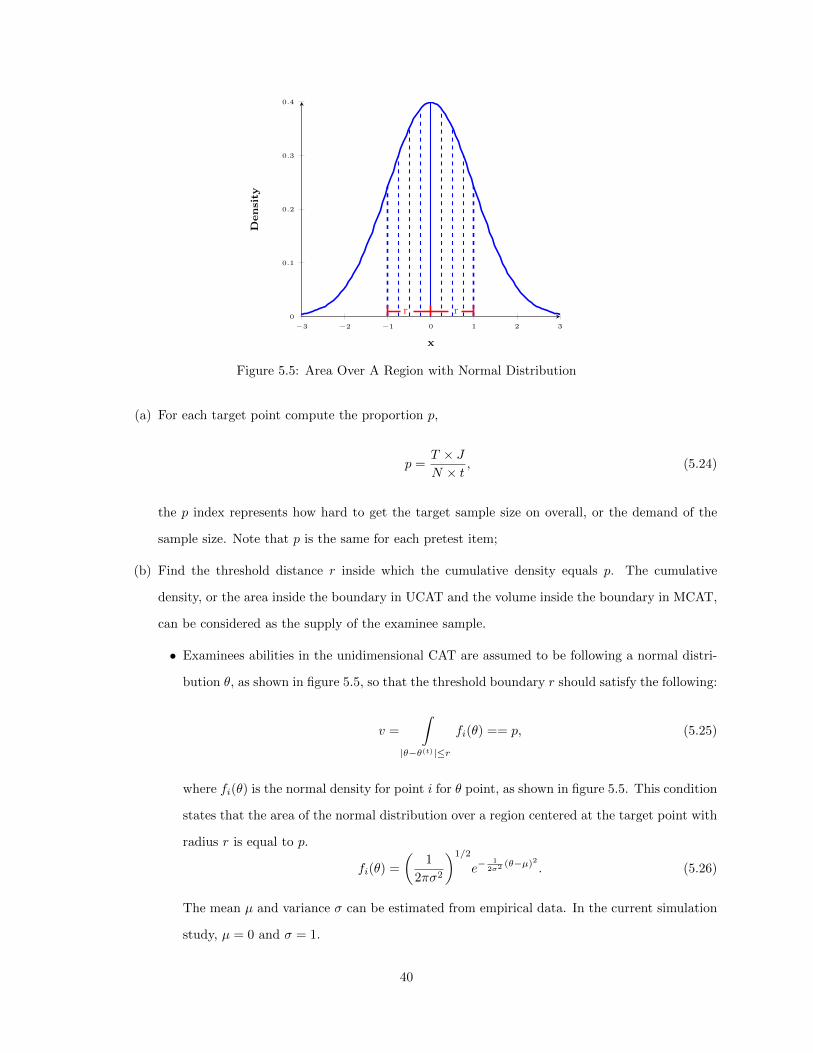
−3 −2 −1 0 1 2 3

0

0.1

0.2

0.3

0.4

r r

x

Density

Figure 5.5: Area Over A Region with Normal Distribution

(a) For each target point compute the proportion p,

p =T × JN × t

, (5.24)

the p index represents how hard to get the target sample size on overall, or the demand of the

sample size. Note that p is the same for each pretest item;

(b) Find the threshold distance r inside which the cumulative density equals p. The cumulative

density, or the area inside the boundary in UCAT and the volume inside the boundary in MCAT,

can be considered as the supply of the examinee sample.

• Examinees abilities in the unidimensional CAT are assumed to be following a normal distri-

bution θ, as shown in figure 5.5, so that the threshold boundary r should satisfy the following:

v =

∫|θ−θ(t)|≤r

fi(θ) == p, (5.25)

where fi(θ) is the normal density for point i for θ point, as shown in figure 5.5. This condition

states that the area of the normal distribution over a region centered at the target point with

radius r is equal to p.

fi(θ) =

(1

2πσ2

)1/2

e−1

2σ2(θ−µ)2 . (5.26)

The mean µ and variance σ can be estimated from empirical data. In the current simulation

study, µ = 0 and σ = 1.

40

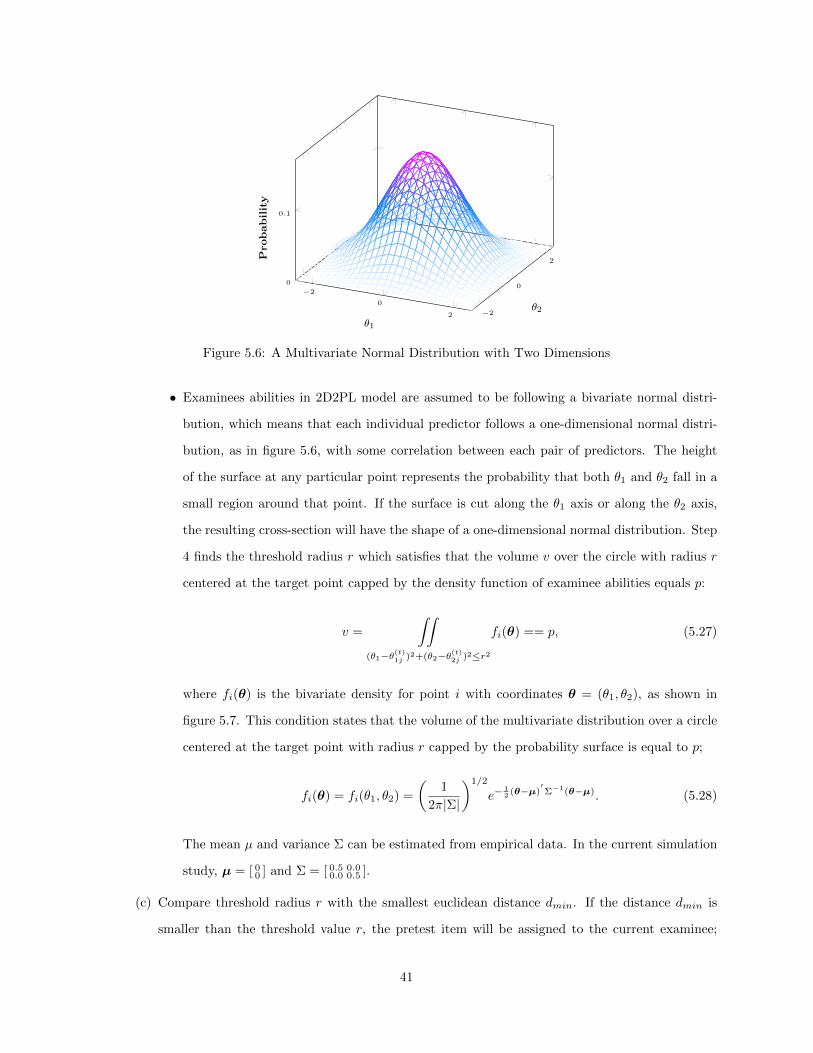
−2

0

2 −2

0

2

0

0.1

θ1

θ2

Probability

Figure 5.6: A Multivariate Normal Distribution with Two Dimensions

• Examinees abilities in 2D2PL model are assumed to be following a bivariate normal distri-

bution, which means that each individual predictor follows a one-dimensional normal distri-

bution, as in figure 5.6, with some correlation between each pair of predictors. The height

of the surface at any particular point represents the probability that both θ1 and θ2 fall in a

small region around that point. If the surface is cut along the θ1 axis or along the θ2 axis,

the resulting cross-section will have the shape of a one-dimensional normal distribution. Step

4 finds the threshold radius r which satisfies that the volume v over the circle with radius r

centered at the target point capped by the density function of examinee abilities equals p:

v =

∫∫(θ1−θ(t)1j )2+(θ2−θ(t)2j )2≤r2

fi(θ) == p, (5.27)

where fi(θ) is the bivariate density for point i with coordinates θ = (θ1, θ2), as shown in

figure 5.7. This condition states that the volume of the multivariate distribution over a circle

centered at the target point with radius r capped by the probability surface is equal to p;

fi(θ) = fi(θ1, θ2) =

(1

2π|Σ|

)1/2

e−12 (θ−µ)

′Σ−1(θ−µ). (5.28)

The mean µ and variance Σ can be estimated from empirical data. In the current simulation

study, µ = [ 00 ] and Σ = [ 0.5 0.0

0.0 0.5 ].

(c) Compare threshold radius r with the smallest euclidean distance dmin. If the distance dmin is

smaller than the threshold value r, the pretest item will be assigned to the current examinee;

41

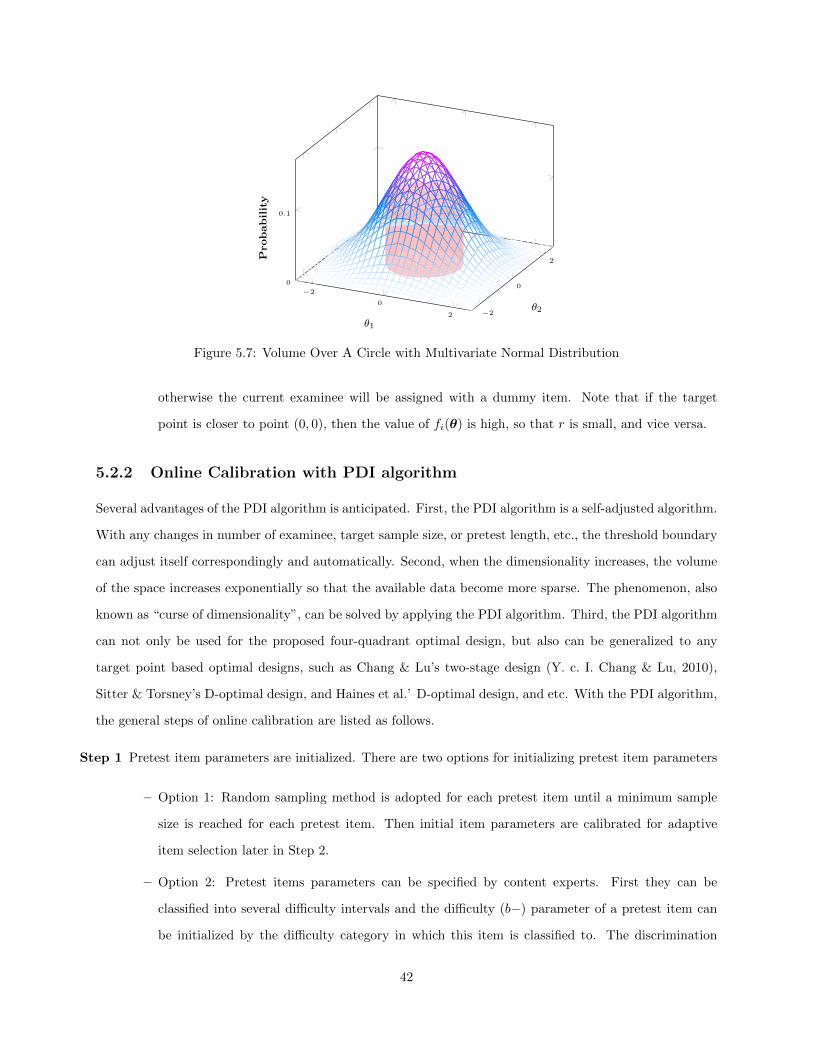
−2

0

2 −2

0

2

0

0.1

θ1

θ2

Probability

Figure 5.7: Volume Over A Circle with Multivariate Normal Distribution

otherwise the current examinee will be assigned with a dummy item. Note that if the target

point is closer to point (0, 0), then the value of fi(θ) is high, so that r is small, and vice versa.

5.2.2 Online Calibration with PDI algorithm

Several advantages of the PDI algorithm is anticipated. First, the PDI algorithm is a self-adjusted algorithm.

With any changes in number of examinee, target sample size, or pretest length, etc., the threshold boundary

can adjust itself correspondingly and automatically. Second, when the dimensionality increases, the volume

of the space increases exponentially so that the available data become more sparse. The phenomenon, also

known as “curse of dimensionality”, can be solved by applying the PDI algorithm. Third, the PDI algorithm

can not only be used for the proposed four-quadrant optimal design, but also can be generalized to any

target point based optimal designs, such as Chang & Lu’s two-stage design (Y. c. I. Chang & Lu, 2010),

Sitter & Torsney’s D-optimal design, and Haines et al.’ D-optimal design, and etc. With the PDI algorithm,

the general steps of online calibration are listed as follows.

Step 1 Pretest item parameters are initialized. There are two options for initializing pretest item parameters

– Option 1: Random sampling method is adopted for each pretest item until a minimum sample

size is reached for each pretest item. Then initial item parameters are calibrated for adaptive

item selection later in Step 2.

– Option 2: Pretest items parameters can be specified by content experts. First they can be

classified into several difficulty intervals and the difficulty (b−) parameter of a pretest item can

be initialized by the difficulty category in which this item is classified to. The discrimination

42

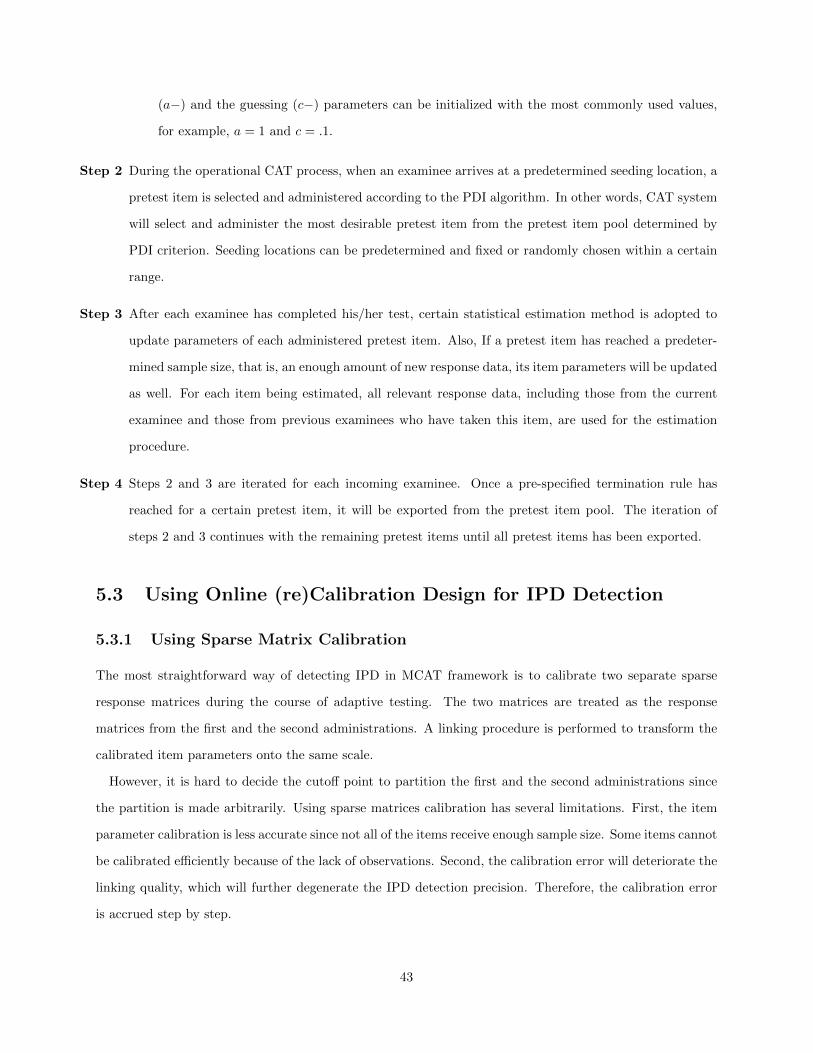
(a−) and the guessing (c−) parameters can be initialized with the most commonly used values,

for example, a = 1 and c = .1.

Step 2 During the operational CAT process, when an examinee arrives at a predetermined seeding location, a

pretest item is selected and administered according to the PDI algorithm. In other words, CAT system

will select and administer the most desirable pretest item from the pretest item pool determined by

PDI criterion. Seeding locations can be predetermined and fixed or randomly chosen within a certain

range.

Step 3 After each examinee has completed his/her test, certain statistical estimation method is adopted to

update parameters of each administered pretest item. Also, If a pretest item has reached a predeter-

mined sample size, that is, an enough amount of new response data, its item parameters will be updated

as well. For each item being estimated, all relevant response data, including those from the current

examinee and those from previous examinees who have taken this item, are used for the estimation

procedure.

Step 4 Steps 2 and 3 are iterated for each incoming examinee. Once a pre-specified termination rule has

reached for a certain pretest item, it will be exported from the pretest item pool. The iteration of

steps 2 and 3 continues with the remaining pretest items until all pretest items has been exported.

5.3 Using Online (re)Calibration Design for IPD Detection

5.3.1 Using Sparse Matrix Calibration

The most straightforward way of detecting IPD in MCAT framework is to calibrate two separate sparse

response matrices during the course of adaptive testing. The two matrices are treated as the response

matrices from the first and the second administrations. A linking procedure is performed to transform the

calibrated item parameters onto the same scale.

However, it is hard to decide the cutoff point to partition the first and the second administrations since

the partition is made arbitrarily. Using sparse matrices calibration has several limitations. First, the item

parameter calibration is less accurate since not all of the items receive enough sample size. Some items cannot

be calibrated efficiently because of the lack of observations. Second, the calibration error will deteriorate the

linking quality, which will further degenerate the IPD detection precision. Therefore, the calibration error

is accrued step by step.

43

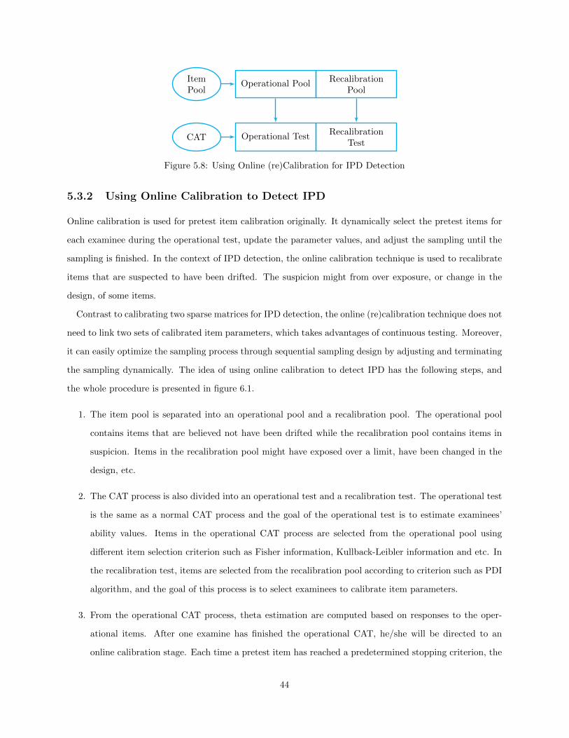
Operational PoolItemPool

RecalibrationPool

Operational TestCATRecalibration

Test

Figure 5.8: Using Online (re)Calibration for IPD Detection

5.3.2 Using Online Calibration to Detect IPD

Online calibration is used for pretest item calibration originally. It dynamically select the pretest items for

each examinee during the operational test, update the parameter values, and adjust the sampling until the

sampling is finished. In the context of IPD detection, the online calibration technique is used to recalibrate

items that are suspected to have been drifted. The suspicion might from over exposure, or change in the

design, of some items.

Contrast to calibrating two sparse matrices for IPD detection, the online (re)calibration technique does not

need to link two sets of calibrated item parameters, which takes advantages of continuous testing. Moreover,

it can easily optimize the sampling process through sequential sampling design by adjusting and terminating

the sampling dynamically. The idea of using online calibration to detect IPD has the following steps, and

the whole procedure is presented in figure 6.1.

1. The item pool is separated into an operational pool and a recalibration pool. The operational pool

contains items that are believed not have been drifted while the recalibration pool contains items in

suspicion. Items in the recalibration pool might have exposed over a limit, have been changed in the

design, etc.

2. The CAT process is also divided into an operational test and a recalibration test. The operational test

is the same as a normal CAT process and the goal of the operational test is to estimate examinees’

ability values. Items in the operational CAT process are selected from the operational pool using

different item selection criterion such as Fisher information, Kullback-Leibler information and etc. In

the recalibration test, items are selected from the recalibration pool according to criterion such as PDI

algorithm, and the goal of this process is to select examinees to calibrate item parameters.

3. From the operational CAT process, theta estimation are computed based on responses to the oper-

ational items. After one examine has finished the operational CAT, he/she will be directed to an

online calibration stage. Each time a pretest item has reached a predetermined stopping criterion, the

44

sampling process is finished, and hypothesis testing such as likelihood ratio test, NCDIF and ect. is

then applied to detect drifted items.

Likelihood ratio testing to detect IPD Thissen, Steinberg, and Gerrard (1986); Thissen, Steinberg,

and Wainer (1988) and Thissen, Steinberg, and Wainer (1993) used likelihood ratio test (LRT) (Neyman

& Pearson, 1928) to detect the difference in response between groups and between test administrations.

Under the IRT framework, S.-H. Kim and Cohen (1995) compared LRT with Lord’s (1980) χ2 test and

Raju’s (1988, 1990) area measures and found results to be comparable. Cohen, Kim, and Wollack (1996)

subsequently reported Type I error rates of LRT under the two− and three− parameter IRT models to be

within expected limits at the nominal alpha (α) levels considered. Witt, Ankenmann, and Dunbar (1996)

compared the power and Type I error rates of the lRT and the Mantel-Haenszel test (Mantel, 1963) under

the graded response model (GRM).

The term likelihood ratio test is originated from the filed of statistics, which is used to compare the

goodness of fit of two nested statistical models. In likelihood ratio test, two models, a null model (Mc) and

an alternative model (Ma) are compared, where the former is a special case of the latter. The general idea is

to compute the likelihood ratio between the null model and the alternative model, and to look at how many

times one model is more likely to occur than the other. To compare the null model with the alternative

model, the deviance statistic is measure by twice the ratio between the likelihood of the null model and that

of the alternative model:

Deviance = −2ln

[L(Mc)

L(Ma)

](5.29)

This deviance value can then be used in the computation of p−value, critical value, the probability distri-

bution of the test statistic and etc. Researchers have proved that the probability distribution of the test

statistic is approximately following a chi-square distribution with degrees of freedom equal to (df2 − df1),

where df1 and df2 are numbers of free parameters in the null and the alternative models, respectively.

The idea of using likelihood ratio test into psychometric testing was first introduced by Thissen et al.

(1986, 1988, 1993). From then on, the approach of ratio test has been widely used in psychometric testing

scenarios to detect differential item functioning (S.-H. Kim & Cohen, 1998; Cohen et al., 1996; Acar &

Kelecioglu, 2010; Setodji, Reise, Morales, Fongwa, & Hays, 2011) and item parameter drifting (Wollack,

Sung, & Kang, 2006; De Ayala, 2013; Du Toit, 2003). The LRT for assessing DIF and IPD described by

Thissen et al. (1988, 1993) is an IRT based approach. This procedure involves comparing the difference

between of two IRT models − a compact model and an augmented model. The hypothesis of the LRT for

detecting IPD is

45

H0 : item j is not drifted, HA : item j is drifted

Each time one item is studied as the augmented model and all item are studied sequentially. Under the

null hypothesis, item parameters are assumed not drifted, with parameters invariant among different groups,

or between two different test administrations over time. The log likelihood of this compact model (Mc) is

denoted as Lc. Under the alternative model, parameters are free to vary among different groups of examinees,

or different testing occasions, and therefore, the likelihood of the augmented model (Ma) is denoted as La.

The likelihood ratio statistic G2 is then −2 times the difference between the log likelihood for the compact

model (LC) and that for the augmented model (LA), which can be written as

G2 = −2ln

[LcLa

]= −2(lnLc − lnLa) = 2logLa − 2logLc. (5.30)

Under the null hypothesis, when the sample size is large enough, the G2 quantity is following a χ2 distribution

with degrees of freedom equal to the difference in the number of free-varying parameters estimated in the

null and alternative models. In other words, the χ2 distribution is evaluated by the number of constraints

used to derived the augmented model. Specifically, in IRT models, the log-likelihood ratio G2 is the ratio

between two log likelihoods, the null model and the alternative model, can be derived as the following:

G2 = −2ln

[LcLa

]= −2ln

[Lj(θ

(j),βcj ,xj)

Lj(θ(j),βaj ,xj)

], (5.31)

where θ(j) is the ability levels of examinees who has taken the jth pretest item, β0j is the parameter value

of item j under the null model Mc, βaj is the parameter value of item j under the alternative model Ma,

and xj) is the response vector of examinees’ who have answered pretest item j. After a few derivations, the

G2 can be written as

G2 = −2ln

[∑j Pcj(θ)

xj (1− Pcj(θ))(1−xj)∑j Paj(θ)

xj (1− Paj(θ))(1−xj)

](5.32)

where Pcj(θ) is the probability of getting a correct answer from examinees who took pretest item j. The

degrees of freedom is the number of difference of free parameters between the null model and the alternative

model. For example, if a 3PL model is used and all of the a−, b− and c− parameters are free to vary under

Ma, then the likelihood ratio is evaluated at 3 degrees of freedom. If a 2PL model is used, then the degrees

of freedom can be set to 2. For a 1PL model, df = 1. In a 2-dimensional IRT model, the degrees of freedom

is 3, which is the number of parameters (a1−, a2− and b−). The advantage of LRT is that it can be applied

to both UIRT and MIRT scenarios, and therefore, is the choice of the current study.

46

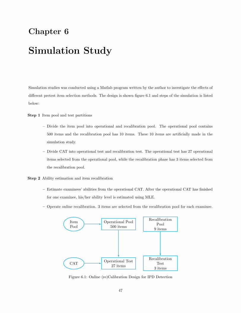
Chapter 6

Simulation Study

Simulation studies was conducted using a Matlab program written by the author to investigate the effects of

different pretest item selection methods. The design is shown figure 6.1 and steps of the simulation is listed

below:

Step 1 Item pool and test partitions

– Divide the item pool into operational and recalibration pool. The operational pool contains

500 items and the recalibration pool has 10 items. These 10 items are artificially made in the

simulation study.

– Divide CAT into operational test and recalibration test. The operational test has 27 operational

items selected from the operational pool, while the recalibration phase has 3 items selected from

the recalibration pool.

Step 2 Ability estimation and item recalibration

– Estimate examinees’ abilities from the operational CAT. After the operational CAT has finished

for one examinee, his/her ability level is estimated using MLE.

– Operate online recalibration. 3 items are selected from the recalibration pool for each examinee.

Operational Pool500 items

ItemPool

RecalibrationPool

9 items

Operational Test27 items

CATRecalibration

Test3 items

Figure 6.1: Online (re)Calibration Design for IPD Detection

47

– Operate likelihood ratio test to detect IPD. For the drifted items, one can either update new

parameter values or retire that item.

6.1 Simulation Designs

Two simulation studies were performed and replicated. The first simulation study was designed under the

UCAT scenario, while the second under a 2D2PL CAT framework. In each simulation study, Four item

selection criteria and three calibration methods were compared and 100 replications were averaged.

6.1.1 Study I: UCAT

Compared Pretest Item Selection Methods Three pretest item selection methods were compared:

(1) random selection, (2) direct comparison of D values, (3) Ali & Chang’s suitability index design, and (4)

modified Chang & Lu’s two-stage design with PDI algorithm.

• Random selection. The random selection condition, which is the easiest method and also the best

possible solution in conventional P & P tests, provides a baseline for the comparison. For a total

number of N examinees and J pretest items, the probability that an examinee is assigned to a pretest

item is given by p = T×JN×t , where p is derived the same as in chapter 5 representing the demand of

examinees. The value of p is expected to be less than 1; otherwise, there are not enough examinees

to calibrate all of the pretest items. Each time a random number u is simulated from a uniform

distribution u U(0, 1) and compared with the value of p. If p < u, then a random selected pretest item

is assigned to the current examinee; otherwise no item is administered.

• Direct comparison of D values. The direct comparison of D value method selects the pretest item that

produces the maximum determinant value. The D value of a pretest item is computed using both the

θ estimate of the current examinee and the θ estimates of all past examinees who took this item.

• Suitability index. Ali & Chang’s suitability index design is compared in the simulation study. The

pretest item that maximizes the weighted difference between difficulty parameter and ability estimates

will be selected, as shown in Equation 4.1.

• Chang & Lu’s Design with PDI algorithm. A modified Chang & Lu’s two-stage design with PDI

algorithm is also compared, as discussed in section 5.2.2. Specifically, the two target points for each

pretest item are b± 1.5434a .

48

Test Specifications The simulation was replicated for 100 times. In each replication, 9 pretest items and

500 operational items were randomly generated from the same distributions. The distributions were chosen

to mimic realistic situations. Specifically,

log(a)

b

∼MVN

0.00

0.00

,0.50 0.00

0.00 0.50

, (6.1)

and

b ∼ N(0, 0.50). (6.2)

In a 2PL UCAT model, c−parameter is equal 0. The current study also checked a 3PL model, with

c−parameter values equal to .2 for all of the operational and recalibration items.

Examinee ability θ’s were generated from a standard normal distribution. In the simulation, examinees

take the CAT test sequentially. The operational items are selected from the operational item bank and the

examinee ability parameter is updated after each operational item is administered. The termination sample

size for each pretest item was 300. Once a pretest item receives a total of 300 examinee responses, it is

exported from the pretest item bank. EAP method was used when the number of administered operational

items is no more than five or the responses are all correct or all incorrect; otherwise, MLE was used.

Similar to the design of Y. c. I. Chang and Lu (2010), the simulation has been separated into two phases:

the normal CAT is first performed to estimate examinees’ abilities and then the pretest phase is aimed at

calibration pretest item parameters. In the pretest CAT phase, examinees whose estimated ability values

have satisfied a pre-specified item selection criterion for a pretest item are selected. Among 9 pretest items,

3 items are simulated to be drifted. Specifically, a− and b−parameters for these items are drifted by adding

.5.

Item Parameter Calibration and Drift Detection Stocking’s Method A was applied in this simulation

and OEM and MEM were also compared. When an examinee reaches the seeding locations, pretest items

are selected from the pretest item bank. From previous study, holding other conditions constant, “late in

the test” seeding locations generated smaller RMSE values for all parameters (Zheng, 2014). Therefore,

pretest items are seeded late in the test. In this simulation study, the test length is 30, and three pretest

items are seeded in items 28 through 30. For IPD detection, the performance of likelihood ratio tests are

also compared under each of the estimation methods using LRT, as described in the previous chapter.

49

Evaluation Criteria By holding the sample sizes constant, the performance of different pretest item

selection methods can be compared by comparing the accuracy of the estimated parameters. The pretest

item selection algorithms are adjusted once the item parameters are updated. The more accurate the

parameter estimates are, the more efficient the methods are. The performance of the compared methods

are evaluated through two criteria. The first criterion focuses on the bias of the individual item parameter

estimates. Specifically, the BIASs of the estimates of each item parameter, formulated by Equation 6.3 are

evaluated.

BIASp =1

J

J∑j=1

abs(βp − βp), (6.3)

where p denotes the specific element in the item parameter vector, such as the a1−parameter, a2− parameter

and b−parameter, and j = 1, 2, ..., J denotes the J pretest items in one replication (J = 9 in this study).

The second criterion focuses on the accuracy of the individual item parameter estimates. Specifically, the

RMSEs of the estimates of each item parameter, formulated by Equation 6.4 are evaluated.

RMSEp =

√√√√ 1

J

J∑j=1

(βp − βp)2. (6.4)

In terms of IPD detection accuracy, type I error rate and power rate are computed separately. To compute

type I error rate α, a null drift condition is simulated without any drifted items, and the type I error rate is

calculated as the proportion of un-drifted items that are falsely flagged as drifted. To compute power rate,

an alternative condition is simulated with drifted items, and the power rate is calculated as the proportion

of items that are correctly flagged as drifted.

α =# of un-drifted items flagged as drifted

J, (6.5)

power =# of drifted items detected

Total # of drifted items. (6.6)

6.1.2 Study II: MCAT

This study differs from the first study in the compared methods, statistical estimation methods and test

specifications.

Compared Pretest Item Selection Methods Four pretest item selection methods were compared: (1)

random selection, (2) direct comparison of D values, (3) Sitter & Torsney’s D-optimal design with PDI

algorithm, and (4) the proposed Four-quadrant D-optimal design with PDI algorithm.

50

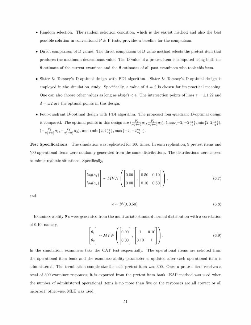
• Random selection. The random selection condition, which is the easiest method and also the best

possible solution in conventional P & P tests, provides a baseline for the comparison.

• Direct comparison of D values. The direct comparison of D value method selects the pretest item that

produces the maximum determinant value. The D value of a pretest item is computed using both the

θ estimate of the current examinee and the θ estimates of all past examinees who took this item.

• Sitter & Torsney’s D-optimal design with PDI algorithm. Sitter & Torsney’s D-optimal design is

employed in the simulation study. Specifically, a value of d = 2 is chosen for its practical meaning.

One can also choose other values as long as abs(d) < 4. The intersection points of lines z = ±1.22 and

d = ±2 are the optimal points in this design.

• Four-quadrant D-optimal design with PDI algorithm. The proposed four-quadrant D-optimal design

is compared. The optimal points in this design are (P∗1

a21+a22a1,

P∗1a21+a22

a2), (max{−2,−2a2a1 },min{2, 2a1a2 }),

(− P∗1a21+a22

a1,− P∗1a21+a22

a2), and (min{2, 2a2a1 },max{−2,−2a1a2 }).

Test Specifications The simulation was replicated for 100 times. In each replication, 9 pretest items and

500 operational items were randomly generated from the same distributions. The distributions were chosen

to mimic realistic situations. Specifically,

log(a1)

log(a2)

∼MVN

0.00

0.00

,0.50 0.10

0.10 0.50

, (6.7)

and

b ∼ N(0, 0.50). (6.8)

Examinee ability θ’s were generated from the multivariate standard normal distribution with a correlation

of 0.10, namely, θ1

θ2

∼MVN

0.00

0.00

, 1 0.10

0.10 1

. (6.9)

In the simulation, examinees take the CAT test sequentially. The operational items are selected from

the operational item bank and the examinee ability parameter is updated after each operational item is

administered. The termination sample size for each pretest item was 300. Once a pretest item receives a

total of 300 examinee responses, it is exported from the pretest item bank. EAP method was used when

the number of administered operational items is no more than five or the responses are all correct or all

incorrect; otherwise, MLE was used.

51

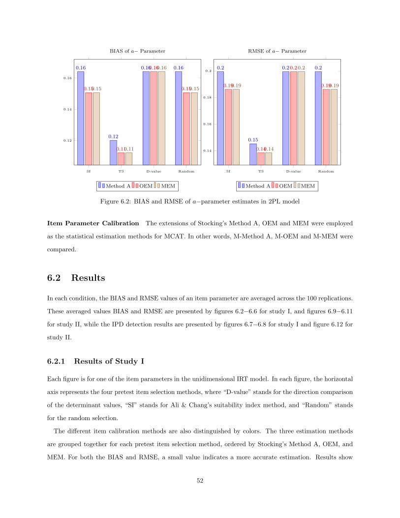
SI TS D-value Random

0.12

0.14

0.16

0.16

0.12

0.16 0.16

0.15

0.11

0.16

0.150.15

0.11

0.16

0.15

BIAS of a− Parameter

Method A OEM MEM

SI TS D-value Random

0.14

0.16

0.18

0.20.2

0.15

0.2 0.2

0.19

0.14

0.2

0.190.19

0.14

0.2

0.19

RMSE of a− Parameter

Method A OEM MEM

Figure 6.2: BIAS and RMSE of a−parameter estimates in 2PL model

Item Parameter Calibration The extensions of Stocking’s Method A, OEM and MEM were employed

as the statistical estimation methods for MCAT. In other words, M-Method A, M-OEM and M-MEM were

compared.

6.2 Results

In each condition, the BIAS and RMSE values of an item parameter are averaged across the 100 replications.

These averaged values BIAS and RMSE are presented by figures 6.2−6.6 for study I, and figures 6.9−6.11

for study II, while the IPD detection results are presented by figures 6.7−6.8 for study I and figure 6.12 for

study II.

6.2.1 Results of Study I

Each figure is for one of the item parameters in the unidimensional IRT model. In each figure, the horizontal

axis represents the four pretest item selection methods, where “D-value” stands for the direction comparison

of the determinant values, “SI” stands for Ali & Chang’s suitability index method, and “Random” stands

for the random selection.

The different item calibration methods are also distinguished by colors. The three estimation methods

are grouped together for each pretest item selection method, ordered by Stocking’s Method A, OEM, and

MEM. For both the BIAS and RMSE, a small value indicates a more accurate estimation. Results show

52

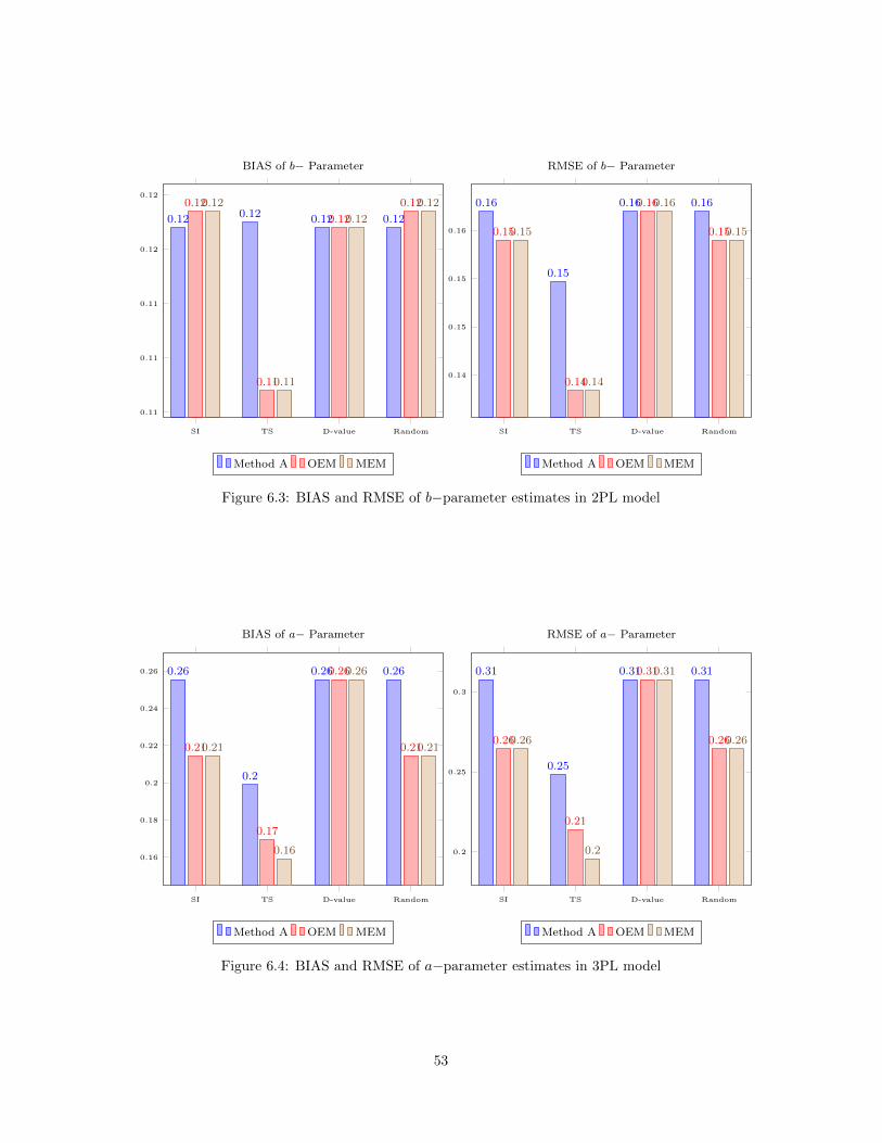
SI TS D-value Random

0.11

0.11

0.11

0.12

0.12

0.12 0.12 0.12 0.12

0.12

0.11

0.12

0.120.12

0.11

0.12

0.12

BIAS of b− Parameter

Method A OEM MEM

SI TS D-value Random

0.14

0.15

0.15

0.16

0.16

0.15

0.16 0.16

0.15

0.14

0.16

0.150.15

0.14

0.16

0.15

RMSE of b− Parameter

Method A OEM MEM

Figure 6.3: BIAS and RMSE of b−parameter estimates in 2PL model

SI TS D-value Random

0.16

0.18

0.2

0.22

0.24

0.26 0.26

0.2

0.26 0.26

0.21

0.17

0.26

0.210.21

0.16

0.26

0.21

BIAS of a− Parameter

Method A OEM MEM

SI TS D-value Random

0.2

0.25

0.3

0.31

0.25

0.31 0.31

0.26

0.21

0.31

0.260.26

0.2

0.31

0.26

RMSE of a− Parameter

Method A OEM MEM

Figure 6.4: BIAS and RMSE of a−parameter estimates in 3PL model

53

SI TS D-value Random

0.17

0.18

0.19

0.2

0.21

0.21

0.19

0.21 0.21

0.19

0.17

0.21

0.190.19

0.17

0.21

0.19

BIAS of b− Parameter

Method A OEM MEM

SI TS D-value Random

0.2

0.22

0.24

0.26

0.26

0.23

0.26 0.26

0.24

0.22

0.26

0.240.24

0.21

0.26

0.24

RMSE of b− Parameter

Method A OEM MEM

Figure 6.5: BIAS and RMSE of b−parameter estimates in 3PL model

SI TS D-value Random

6

7

8

9

·10−2

8.85 · 10−2

6.27 · 10−2

8.85 · 10−2 8.85 · 10−28.85 · 10−2

6.27 · 10−2

8.85 · 10−2 8.85 · 10−28.85 · 10−2

6.62 · 10−2

8.85 · 10−2 8.85 · 10−2

BIAS of c− Parameter

Method A OEM MEM

SI TS D-value Random

6.5

7

7.5

8

8.5

9

·10−2

8.85 · 10−2

6.88 · 10−2

8.85 · 10−2 8.85 · 10−28.85 · 10−2

6.88 · 10−2

8.85 · 10−2 8.85 · 10−28.85 · 10−2

6.62 · 10−2

8.85 · 10−2 8.85 · 10−2

RMSE of c− Parameter

Method A OEM MEM

Figure 6.6: BIAS and RMSE of c−parameter estimates in 3PL model

54

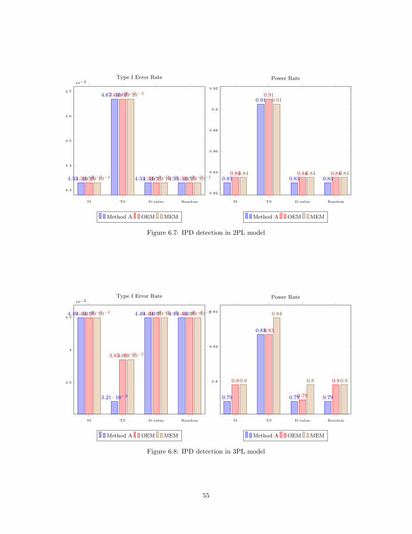
SI TS D-value Random

4.3

4.4

4.5

4.6

4.7

·10−2

4.33 · 10−2

4.67 · 10−2

4.33 · 10−2 4.33 · 10−24.33 · 10−2

4.67 · 10−2

4.33 · 10−2 4.33 · 10−24.33 · 10−2

4.67 · 10−2

4.33 · 10−2 4.33 · 10−2

Type I Error Rate

Method A OEM MEM

SI TS D-value Random

0.82

0.84

0.86

0.88

0.9

0.92

0.83

0.91

0.83 0.830.84

0.91

0.84 0.840.84

0.91

0.84 0.84

Power Rate

Method A OEM MEM

Figure 6.7: IPD detection in 2PL model

SI TS D-value Random

3.5

4

4.5

·10−2

4.49 · 10−2

3.21 · 10−2

4.49 · 10−2 4.49 · 10−24.49 · 10−2

3.85 · 10−2

4.49 · 10−2 4.49 · 10−24.49 · 10−2

3.85 · 10−2

4.49 · 10−2 4.49 · 10−2

Type I Error Rate

Method A OEM MEM

SI TS D-value Random

0.8

0.82

0.84

0.79

0.83

0.79 0.79

0.8

0.83

0.79

0.80.8

0.84

0.8 0.8

Power Rate

Method A OEM MEM

Figure 6.8: IPD detection in 3PL model

55

that in different pretest item selection methods and item calibration methods the patterns of the BIASs and

the RMSEs produced are not the same.

Comparing Calibration Designs The four pretest item selection methods are compared. In figure 6.2,

the D-value method generated the lowest estimation efficiency in terms of bias and RMSE for 2PL IRT

model, perhaps because it is the most greedy algorithm. The D-value method first computes determinant

values of each pretest item, then selects the one with the largest determinant value. However, some items will

always have relatively higher determinant values than other items, no matter which θ values are computed

from. As a result, the D-value method will always select items with higher determinant values until theses

items have received enough target sample size, and then, the method begins to select items with lower

determinant value items, which makes the item assignment highly imbalanced because given limited sample

size, the subsequent pretest items cannot find their ideal examinees because the antecedent ones have already

chosen them.

The estimation efficiency of the SI design is similar to random selection design. One possible reason is

that in the design of Ali and Chang (2011), the weighting strategy of each θ interval is not mentioned in

detail, leaving the current simulation study with an assumption that each θ interval has the same weight.

The two-stage design with PDI algorithm had the best performance in terms of bias and RMSE, indicating

that the PDI a good implementation of the two-stage D-optimal design.

Figure 6.3 compared item calibration results for a 2PL UCAT model in terms of b−parameter estimation

efficiency. The same pattern as for a−parameter has been observed. The two-stage design with the PDI

algorithm had the best performance, followed by the SI design and random assignment. D-value method

had the worst performance as expected.

Figures 6.4 through 6.6 compared item calibration efficiency for a 3PL UCAT model in terms of bias and

RMSE for a−, b− and c−parameter values. For the calibration efficiency of a− and b−parameters, similar

pattern has been observed as in the 2PL UCAT model. It is obvious to see that the D-value method had

the worst performance because it is a greedy algorithm. SI and random assignment generally had similar

performance, and the two-stage design with PDI algorithm had the lowest BIAS and RMSE compared to the

other three. According to figure 6.6, c−parameter estimation efficiency were very similar among all of the

four item selection criteria, with variation from .062 to .085. Since in a 3PL UCAT model, the target point of

estimating c−parameter is − inf, the two-stage optimal design does not take the estimation of c−parameters

into consideration.

56

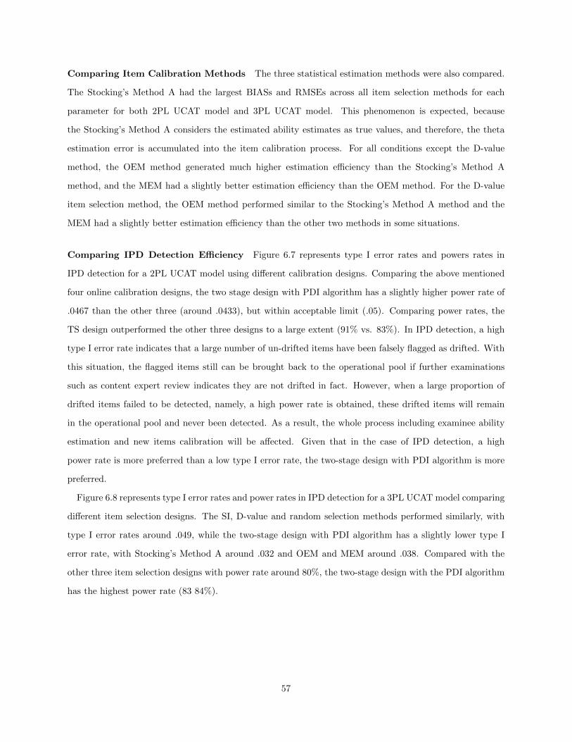
Comparing Item Calibration Methods The three statistical estimation methods were also compared.

The Stocking’s Method A had the largest BIASs and RMSEs across all item selection methods for each

parameter for both 2PL UCAT model and 3PL UCAT model. This phenomenon is expected, because

the Stocking’s Method A considers the estimated ability estimates as true values, and therefore, the theta

estimation error is accumulated into the item calibration process. For all conditions except the D-value

method, the OEM method generated much higher estimation efficiency than the Stocking’s Method A

method, and the MEM had a slightly better estimation efficiency than the OEM method. For the D-value

item selection method, the OEM method performed similar to the Stocking’s Method A method and the

MEM had a slightly better estimation efficiency than the other two methods in some situations.

Comparing IPD Detection Efficiency Figure 6.7 represents type I error rates and powers rates in

IPD detection for a 2PL UCAT model using different calibration designs. Comparing the above mentioned

four online calibration designs, the two stage design with PDI algorithm has a slightly higher power rate of

.0467 than the other three (around .0433), but within acceptable limit (.05). Comparing power rates, the

TS design outperformed the other three designs to a large extent (91% vs. 83%). In IPD detection, a high

type I error rate indicates that a large number of un-drifted items have been falsely flagged as drifted. With

this situation, the flagged items still can be brought back to the operational pool if further examinations

such as content expert review indicates they are not drifted in fact. However, when a large proportion of

drifted items failed to be detected, namely, a high power rate is obtained, these drifted items will remain

in the operational pool and never been detected. As a result, the whole process including examinee ability

estimation and new items calibration will be affected. Given that in the case of IPD detection, a high

power rate is more preferred than a low type I error rate, the two-stage design with PDI algorithm is more

preferred.

Figure 6.8 represents type I error rates and power rates in IPD detection for a 3PL UCAT model comparing

different item selection designs. The SI, D-value and random selection methods performed similarly, with

type I error rates around .049, while the two-stage design with PDI algorithm has a slightly lower type I

error rate, with Stocking’s Method A around .032 and OEM and MEM around .038. Compared with the

other three item selection designs with power rate around 80%, the two-stage design with the PDI algorithm

has the highest power rate (83 84%).

57

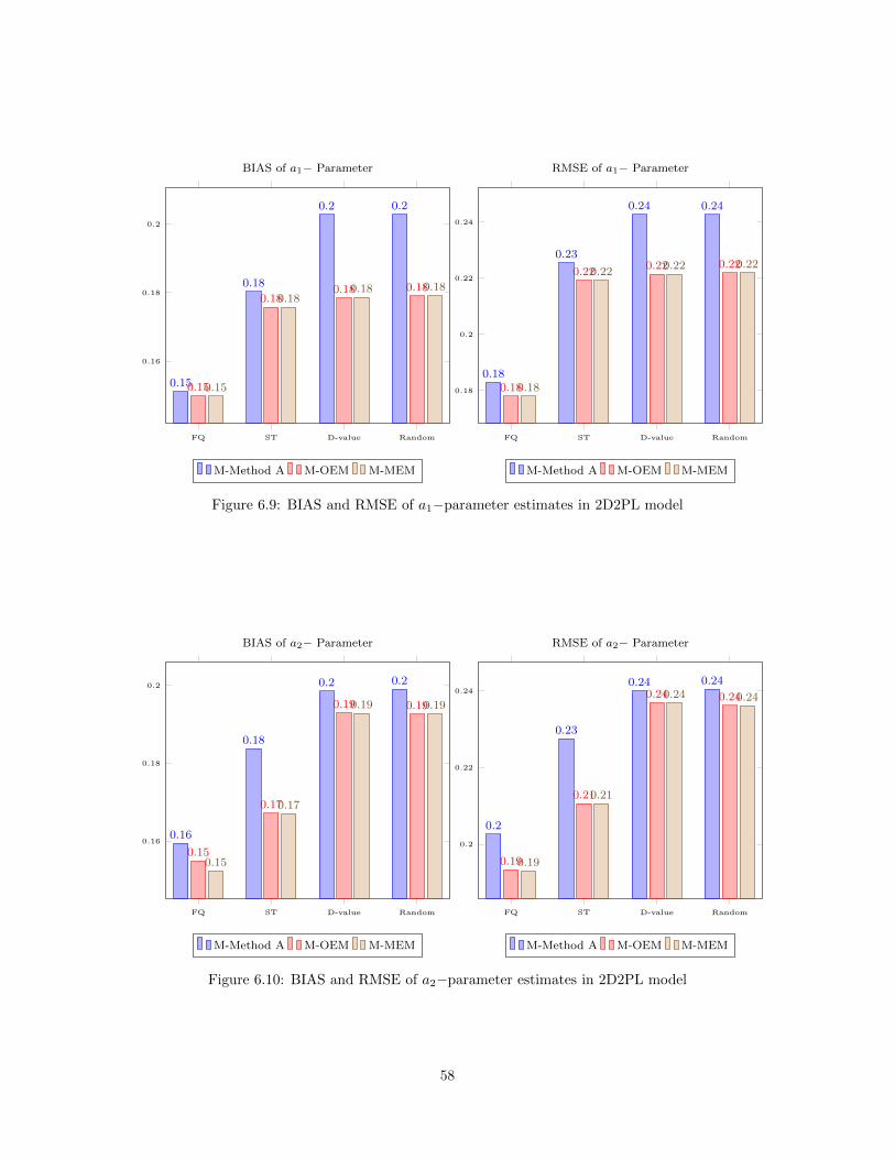
FQ ST D-value Random

0.16

0.18

0.2

0.15

0.18

0.2 0.2

0.15

0.180.18 0.18

0.15

0.180.18 0.18

BIAS of a1− Parameter

M-Method A M-OEM M-MEM

FQ ST D-value Random

0.18

0.2

0.22

0.24

0.18

0.23

0.24 0.24

0.18

0.220.22 0.22

0.18

0.220.22 0.22

RMSE of a1− Parameter

M-Method A M-OEM M-MEM

Figure 6.9: BIAS and RMSE of a1−parameter estimates in 2D2PL model

FQ ST D-value Random

0.16

0.18

0.2

0.16

0.18

0.2 0.2

0.15

0.17

0.19 0.19

0.15

0.17

0.19 0.19

BIAS of a2− Parameter

M-Method A M-OEM M-MEM

FQ ST D-value Random

0.2

0.22

0.24

0.2

0.23

0.24 0.24

0.19

0.21

0.24 0.24

0.19

0.21

0.24 0.24

RMSE of a2− Parameter

M-Method A M-OEM M-MEM

Figure 6.10: BIAS and RMSE of a2−parameter estimates in 2D2PL model

58

FQ ST D-value Random

0.12

0.12

0.12

0.12

0.13

0.13

0.13

0.13

0.12

0.13

0.12

0.12

0.12

0.120.12

0.12

0.12

0.12

BIAS of b− Parameter

M-Method A M-OEM M-MEM

FQ ST D-value Random

0.15

0.15

0.15

0.15

0.16

0.16

0.16 0.16

0.16

0.15

0.15

0.15

0.15

0.15

0.15

0.15

0.15

0.15

RMSE of b− Parameter

M-Method A M-OEM M-MEM

Figure 6.11: BIAS and RMSE of b−parameter estimates in 2D2PL model

FQ ST D-value Random

1

2

3

4

·10−2

3.6 · 10−2

2.4 · 10−2

6 · 10−3

3.2 · 10−23.4 · 10−2

2 · 10−2

8 · 10−3

3.8 · 10−2

3.4 · 10−2

2 · 10−2

8 · 10−3

4 · 10−2

Type I Error Rate

M-Method A M-OEM M-MEM

FQ ST D-value Random

0.7

0.75

0.8

0.85

0.82

0.68 0.68

0.74

0.84

0.77

0.7

0.78

0.84

0.77

0.7

0.78

Power Rate

M-Method A M-OEM M-MEM

Figure 6.12: IPD detection in 2D2PL model

59

6.2.2 Results of Study II

In study II, a 2D2PL model is examined in terms of item calibration efficiency and IPD detection efficiency,

with corresponding figures 6.9 through 6.11. Each figure is for one of the item parameters, a1−, a2− and b−,

in the 2D2PL model. In each figure, the horizontal axis represents the four pretest item selection methods,

where “D-value” stands for the direction comparison of the determinant values, “ST” stands for Sitter &

Torsney’s D-optimal design with PDI algorithm, “FQ” stands for the proposed four-quadrant D-optimal

design with PDI algorithm, and “Random” stands for the random selection with filter probability p = T×JN×t .

Different item calibration methods are distinguished by colors as in study I. The three estimation methods

are grouped together for each pretest item selection method, ordered by M-Method A, M-OEM, and M-

MEM. For both the BIAS and RMSE, a small value indicates a more accurate estimation. Results show

that in different pretest item selection methods and item calibration methods the patterns of the BIASs and

the RMSEs produced are not the same.

Comparing Calibration Designs Four pretest item selection methods are compared. The FQ design

with PDI algorithm generated the smallest BIAS and RMSE values in general, which means that it is the

most efficient design. The direct D-value selection method generates the lowest estimation efficiency perhaps

because of it is the most greedy algorithm. Given limited sample size, the subsequent pretest items cannot

find their ideal examinees because the antecedent ones have already chosen them. The estimation efficiency

of the ST design is better than the direction D-value method but worse than the random selection, which is

expected, because the design space of this method cannot be fully applied in the 2D2PL situation.

Figure 6.9 shows that the FQ design with PDI algorithm generated the smallest BIAS value for

a1−parameter across different estimation methods, which means the most efficient calibration. It is more

efficient than the other three methods. The performance of a2−parameter, shown by figure 6.10, has the

similar pattern for all of the item selection method, which is expected, because they are counterparts in the

2D2PL model. However, the pattern of the b−parameter across different item selection methods is different

from a−parameters. Figure 6.11 indicates the estimation bias for b−parameter, which shows that the FQ,

ST, D-value and the Random methods have equivalent efficiency with respect to b−parameter estimation.

Comparing Item Calibration Methods The three statistical estimation methods are also compared.

The M-Method A has the largest BIASs and RMSEs across all item selection methods for each parameter.

This phenomenon is expected, because the M-Method A considers the estimated ability estimates as true

values. For all conditions expect the D-value method, the M-OEM method generates much higher estimation

efficiency than the M-Method A method, and the M-MEM has a slightly but not obvious better estimation

60

efficiency than the M-OEM method. For the D-value item selection method, the M-OEM method performs

similar to the M-Method A method and the M-MEM has a slightly better estimation efficiency than the

other two methods.

Therefore, one thing consistent across all conditions is that the M-MEM method appears to be the most

stable method among the three and in most cases generated the smallest BIASs and RMSEs. Therefore,

the M-MEM method is recommended in general, and all following analyses are conducted using the data

generated from the M-MEM method only.

Comparing IPD Detection Results Figure 6.12 shows the two types of errors in parameter drift de-

tection using different calibration designs. Comparing the above mentioned four online calibration designs,

the D-value method had the smallest type I error rate, but also had the smallest power rate. The FQ design

with PDI algorithm had a relatively high type I error rate, and the highest power rate. The ST design with

PDI algorithm had a slightly smaller type I error rate and power rate compared to FQ design, while the

random design had the largest type I error rate with power rate in between. As mentioned before, in the

case of IPD detection, a higher power rate is more preferred than a lower type I error as long as the type I

error rate is within acceptable limit. Therefore, the FQ is the most efficient design.

6.2.3 Conclusions

In summary, the following conclusions can be made within the settings of the current simulation study:

1. Using online calibration technique is more desirable way to detect IPD compared to traditional sparse

matrix calibration under computerized adaptive testing framework. By implementing online calibration

to detect IPD, more items can be recalibrated, and therefore, higher calibration efficiency and IPD

detection accuracy could be obtained.

2. Under the unidimensional IRT model, the two-stage design with proportional density index is the most

efficient method in terms of BIAS, RMSE, type I error rate and power rate.

3. Under the two-dimensional IRT model, The proposed new four-quadrant D-optimal design with pro-

portional density index is the most efficient item selection method for online calibration.

4. The performance of the direct comparison of D value is not satisfactory since it is a greedy algorithm.

5. Comparing three estimation methods, the conditional maximum likelihood estimation has the lowest

estimation efficiency, and two bayesian based estimation method, OEM (M-OEM) and MEM (M-MEM)

methods, have similar performance.

61

6. The proposed FQ design can not only be used in the framework of IPD detection for CAT, but also

can be used for the general online calibration of pretest items.

62

Chapter 7

Discussion

7.1 Conclusions

Computerized adaptive testing has gained an increasing popularity in recent years. Many large-scale testing

programs have switched from P&P testing mode to computer based testing mode. CAT selects operational

items to match the current ability estimate of examinees, and provides a great solution to large-scale cali-

bration due to the nature of “online” and “sequential”. The major advantage of CAT is that it offers more

efficient latent trait estimates and requires fewer operational items than in a P&P test.

There are at least two motivations for developing multidimensional computerized adaptive testing. First,

unidimensional models do not fit for some educational and psychological tests which measure more than

one ability. Multidimensional response models are needed in order to satisfy the assumption of local in-

dependence. MIRT models offers diagnostic information and allows correlation between traits on different

dimensions. Therefore, it is more realistic. The second motivation is that MCAT makes the ability estima-

tion process more efficient because information from correlated abilities can be borrowed (Yao, Center, Bay,

& Yao, 2013).

Item replenishing and item pool maintenance is crucial for item bank construction in both UCAT and

MCAT because estimation efficiency of examinees’ ability levels are affected by the calibration precision

of new items. What’s more, other components of IRT based tests also depend on a well calibrated item

bank, such as scoring, equating, DIF analysis and item selection in adaptive test. Item calibration is used

for constructing new item bank, replenishing the existing item bank, recalibrating items, and performing

equating, linking and vertical scaling as well, making the new items calibration a technical challenge. In

fact, CAT offers the unique opportunity to assign different pretest items to each examinee adaptively.

On the one hand, one important issue of CAT is item bank maintaining by item parameter drift detecting

and parameter updating for drifted items. Previous methods of IPD detection used separate item calibration

and linking method to detect drifted item. Since online calibration technique is commonly used to calibrate

the new items, it can also be used to recalibrate existing items and detect IPD.

63

On the other hand, studies on online calibration for traditional UCAT is reviewed with focus on adaptive

pretest item selection design. There have been relatively abundant research results for the traditional UCAT.

However, until now few reference has publicly become available about online calibration pretest item selection

for MCAT. Thus, this study also investigates the possibility to develop an optimal pretest item selection

method for MCAT. Specifically, a four-quadrant D-optimal design is proposed and to make all of the target-

point based optimal designs fit the real practice, a proportional density index algorithm is also developed

to modify the two-stage design proposed by Y. c. I. Chang and Lu (2010) in UCAT and four-quadrant

D-optimal design in MCAT.

Results show that using online calibration to detect IPD can improve IPD detection efficiency than tradi-

tional sparse matrix calibration. In addition, the proposed modified two-stage optimal design with the PDI

algorithm in UCAT and the four-quadrant D-optimal design with the PDI algorithm in MCAT can improve

item parameter recovery efficiency than other pretest item selection design, thus improve the IPD detection

process.

7.2 Future Directions

There are several limitations in the current simulation study. One limitation is that the results and con-

clusions from the simulation study are limited within the current simulation design, and therefore, the

generalizability under other simulation conditions and real test situations of the proposed method is worth

investigating. The second limitation is that the current simulation study fixed the sample sizes for all pretest

items. In the future, termination rules based on measurement accuracy can be developed as well. Some

other future directions are listed below.

High-dimensional model The current study only explored the optimal design for a two dimensional

two parameter item response model. The model is essentially a logistic model with two design variables.

However, the optimal design for models with number of variables more than two is a big challenge, which

may require complicated mathematical derivations.

Polytomous models In test situations where a partial credits is allowed, polytomous IRT models is

applied. Zheng (2015) explored online calibration of polytomous models in computerized adaptive testing

in a unidimensional CAT case. In the future, a multidimensional CAT model with partial credits can be

examined as well.

64

Multistage testing Multistage testing is group-based approach to administering tests. Different to com-

puterized adaptive testing where individual item is selected based previous responses, multistage testing

selects a group of items each time. These groups are called testlets or panels. Given the fact that multi-

stage testing are widely implemented and studied testing programs by researchers and practitioners (Zheng,

Nozawa, Gao, & Chang, 2012; Zheng & Chang, 2014, 2015; S. Wang, Lin, Chang, & Douglas, 2016)

CAT with response revision One controversial issue related to CAT is whether CAT should allow ex-

aminees to change answer. As presented in S. Wang, Fellouris, and Chang (under revisiona) and S. Wang,

Fellouris, and Chang (under revisionb), a CAT design is introduced that preserves the efficiency of a con-

ventional CAT, but allows test-takers to revise their previous answers at any time during the test, which

has been proven that could reduce measurement error and is robust against several well-known test-taking

strategies. Future research could be conducted to explore the outcome of using this CAT design into online

calibration stage instead of in operational CAT only.

Non-compensatory models Rather than compensatory model used in this study, another category of

MIRT models are non-compensatory models, or conjunctive models, where a poor ability on one dimension

will lead to a low chance of getting a correct answer irrespective of other dimensions. An example of the

conjunctive model is shown in the following equation, where a correct response requires a high ability value

on all dimensions. The optimal design for non-compensatory model is an interesting topic in the future

study.

P (θi) =

M∏m=1

exp(θim − bm)

1 + exp(θim − bm)(7.1)

Other optimal criterion The current study used D-optimal method as the optimality criterion only. In

the future, other optimality criterion can be examined. A comprehensive list of optimal criteria are shown

in the following

• A-optimality: minimize the trace of the inverse of the information matrix

• E-optimality: maximizes the minimum eigenvalue of the information matrix

• C-optimality: minimizes the variance of a best linear unbiased estimator of a predetermined linear

combination of model parameters

• T-optimality: maximizes the trace of the information matrix

65

• G-optimality: minimize the maximum entry in the diagonal of the hat matrix X(X ′X)−1X ′

• I-optimality: minimize the average prediction variance over the design space

• V-optimality: minimize the average prediction variance over a set of m specific points

Practical Implementations The online calibration design and IPD detection technique can be easily

implemented into large-scale testing programs. For example, the Confucius Institute (CI) in the University of

Illinois at Urbana-Champaign (UIUC) is developing a online computerized adaptive based testing programing

for HSK, a Chinese language proficiency testing. In the process of transferring HSK from P&P to CAT,

S. Wang, Zheng, Zheng, Su, and Li (in press) first calibrated item parameters from previous item responses,

a research group in CI of UIUC is developing a real online based CAT platform that supports both adaptive

test and online calibration.

66

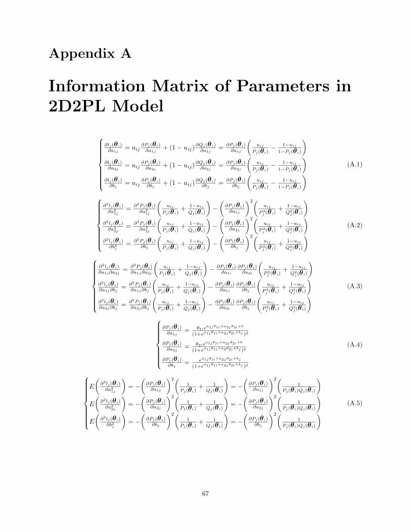
Appendix A

Information Matrix of Parameters in2D2PL Model

∂lj(θi)∂a1j

= uij∂Pj(θi)∂a1j

+ (1− uij)∂Qj(θi)∂a1j=

∂Pj(θi)∂a1j

(uij

Pj(θi)− 1−uij

1−Pj(θi)

)∂lj(θi)∂a2j

= uij∂Pj(θi)∂a2j

+ (1− uij)∂Qj(θi)∂a2j=

∂Pj(θi)∂a2j

(uij

Pj(θi)− 1−uij

1−Pj(θi)

)∂lj(θi)∂bj

= uij∂Pj(θi)∂bj

+ (1− uij)∂Qj(θi)∂bj=

∂Pj(θi)∂bj

(uij

Pj(θi)− 1−uij

1−Pj(θi)

) (A.1)

∂2lj(θi)∂a21j

=∂2Pj(θi)∂a21j

(uij

Pj(θi)+

1−uijQj(θi)

)−(∂Pj(θi)∂a1j

)2(uij

P 2j (θi)

+1−uijQ2j (θi)

)∂2lj(θi)∂a22j

=∂2Pj(θi)∂a22j

(uij

Pj(θi)+

1−uijQj(θi)

)−(∂Pj(θi)∂a2j

)2(uij

P 2j (θi)

+1−uijQ2j (θi)

)∂2lj(θi)∂b2j

=∂2Pj(θi)∂bj

(uij

Pj(θi)+

1−uijQj(θi)

)−(∂Pj(θi)∂bj

)2(uij

P 2j (θi)

+1−uijQ2j (θi)

) (A.2)

∂2lj(θi)∂a1j∂a2j

=∂2Pj(θi)∂a1j∂a2j

(uij

Pj(θi)+

1−uijQj(θi)

)− ∂Pj(θi)

∂a1i

∂Pj(θi)∂a2i

(uij

P 2j (θi)

+1−uijQ2j (θi)

)∂2lj(θi)∂a1j∂bj

=∂2Pj(θi)∂a1j∂bj

(uij

Pj(θi)+

1−uijQj(θi)

)− ∂Pj(θi)

∂a1i

∂Pj(θi)∂bj

(uij

P 2j (θi)

+1−uijQ2j (θi)

)∂2lj(θi)∂a2j∂bj

=∂2Pj(θi)∂a2j∂bj

(uij

Pj(θi)+

1−uijQj(θi)

)− ∂Pj(θi)

∂a2i

∂Pj(θi)∂bj

(uij

P 2j (θi)

+1−uijQ2j (θi)

) (A.3)

∂Pj(θi)∂a1j

= θ1iea1jθ1i+a2jθ2i+b

(1+ea1jθ1i+a2jθ2i+bj )2

∂Pj(θi)∂a2j

= θ2iea1jθ1i+a2jθ2i+b

(1+ea1jθ1i+a2θ2i+bj )2

∂Pj(θi)∂bj

= ea1jθ1i+a2jθ2i+bj

(1+ea1jθ1i+a2jθ2i+bj )2

(A.4)

E

(∂2lj(θi)∂a21j

)= −

(∂Pj(θi)∂a1j

)2(1

Pj(θi)+ 1

Qj(θi)

)= −

(∂Pj(θi)∂a1j

)2(1

Pj(θi)Qj(θi)

)E

(∂2lj(θi)∂a22j

)= −

(∂Pj(θi)∂a2j

)2(1

Pj(θi)+ 1

Qj(θi)

)= −

(∂Pj(θi)∂a2j

)2(1

Pj(θi)Qj(θi)

)E

(∂2lj(θi)∂b2j

)= −

(∂Pj(θi)∂bj

)2(1

Pj(θi)+ 1

Qj(θi)

)= −

(∂Pj(θi)∂bj

)2(1

Pj(θi)Qj(θi)

) (A.5)

67

E

(∂2lj(θi)∂a1j∂a2j

)= −∂Pj(θi)∂a1j

∂Pj(θi)∂a2j

(1

Pj(θi)+ 1

Qj(θi)

)= −∂Pj(θi)∂a1j

∂Pj(θi)∂a2j

(1

Pj(θi)Qj(θi)

)E

(∂2lj(θi)∂a1j∂bj

)= −∂Pj(θi)∂a1j

∂Pj(θi)∂bj

(1

Pj(θi)+ 1

Qj(θi)

)= −∂Pj(θi)∂a1j

∂Pj(θi)∂bj

(1

Pj(θi)Qj(θi)

)E

(∂2lj(θi)∂a2j∂bj

)= −∂Pj(θi)∂a2j

∂Pj(θi)∂bj

(1

Pj(θi)+ 1

Qj(θi)

)= −∂Pj(θi)∂a2j

∂Pj(θi)∂bj

(1

Pj(θi)Qj(θi)

) (A.6)

Ij(θi) =

Ia1ja1j

Ia2ja1j Ia2ja2j

Ibjaa1j Ibja2j Ibjbj

= Pj(θi)Qj(θi)

θ2

1i

θ1iθ2i θ22i

θ1i θ2i 1

(A.7)

68

References

Acar, T., & Kelecioglu, H. (2010). Comparison of differential item functioning determination techniques:Hglm, lr and irt-lr. Educational Sciences: Theory and Practice, 10 (2), 639–649.

Ackerman, T. (1996). Graphical representation of multidimensional item response theory analyses. AppliedPsychological Measurement , 20 (4), 311–329.

Ali, U. S., & Chang, H.-h. (2011). Online calibration design for pretesting items in adaptive testing. HongKong, China.

Allen, M. J., & Yen, W. M. (2001). Introduction to measurement theory. Waveland Press.Baker, F. B., & Kim, S.-H. (2004). Item response theory: Parameter estimation techniques. CRC Press.Ban, J. C., Hanson, B. A., Wang, T., Yi, Q., & Harris, D. J. (2001). A comparative study of online

pretest itemcalibration/scaling methods in computerized adaptive testing. Journal of EducationalMeasurement , 38 (3), 191–212.

Berger, M. P. (1991). On the efficiency of IRT models when applied to different sampling designs. AppliedPsychological Measurement , 15 (3), 293–306.

Berger, M. P. (1992). Sequential sampling designs for the two-parameter item response theory model.Psychometrika, 57 (4), 521–538.

Berger, M. P., King, C. J., & Wong, W. K. (2000). Minimax d-optimal designs for item response theorymodels. Psychometrika, 65 (3), 377–390.

Berger, M. P., & Wong, W. K. (2005). Applied optimal designs. Wiley Online Library.Birnbaum, A. (1968). Some latent trait models and their use in inferring an examinee’s ability. Statistical

theories of mental test scores.Bolt, D. M., & Lall, V. F. (2003). Estimation of compensatory and noncompensatory multidimensional

item response models using markov chain monte carlo. Applied Psychological Measurement , 27 (6),395–414.

Buyske, S. (2005). Optimal design in educational testing. Applied optimal designs, 1–19.Chang, H.-h. (2012). Making computerized adaptive testing diagnostic tools for schools. Computers and

their impact on state assessment: Recent history and predictions for the future, 195–226.Chang, H.-h., Qian, J., & Ying, Z. (2001). a-stratified multistage computerized adaptive testing with b

blocking. Applied Psychological Measurement , 25 (4), 333–341.Chang, H.-h., & Ying, Z. (1996). A global information approach to computerized adaptive testing. Applied

Psychological Measurement , 20 (3), 213–229.Chang, H.-h., & Ying, Z. (1999). A-stratified multistage computerized adaptive testing. Applied Psychological

Measurement , 23 (3), 211–222.Chang, H.-h., & Ying, Z. (2009). Nonlinear sequential designs for logistic item response theory models with

applications to computerized adaptive tests. The Annals of Statistics, 1466–1488.Chang, Y.-c. I. (2011). Sequential estimation in generalized linear models when covariates are subject to

errors. Metrika, 73 (1), 93–120.Chang, Y. c. I., & Lu, H. Y. (2010). Online calibration via variable length computerized adaptive testing.

Psychometrika, 75 (1), 140–157.Chen, P., Xin, T., Wang, C., & Chang, H. H. (2012). Online calibration methods for the dina model with

independent attributes in cd-cat. Psychometrika, 77 (2), 201–222.Chen, P., Zhang, J., & Xin, T. (2013). Application of online calibration technique in computerized adaptive

testing. Advances in Psychological Science, 21 (10), 1883-1892.

69

Cheng, Y., & Yuan, K. H. (2010). The impact of fallible item parameter estimates on latent trait recovery.Psychometrika, 75 (2), 280–291.

Cohen, A. S., Kim, S.-H., & Wollack, J. A. (1996). An investigation of the likelihood ratio test for detectionof differential item functioning. Applied Psychological Measurement , 20 (1), 15–26.

Cook, R. D., & Weisberg, S. (2009). Applied regression including computing and graphics. New York, NY:John Wiley & Sons.

De Ayala, R. J. (2013). Theory and practice of item response theory. Guilford Publications.de la Torre, J., & Patz, R. J. (2005). Making the most of what we have: A practical application of

multidimensional item response theory in test scoring. Journal of Educational and Behavioral Statistics,30 (3), 295–311.

Du Toit, M. (2003). Irt from ssi: Bilog-mg, multilog, parscale, testfact. Scientific Software International.Embretson, S. E., & Yang, X. (2013). A multicomponent latent trait model for diagnosis. Psychometrika,

78 (1), 14–36.Folk, B. G., & Golub-Simith, M. (1996). Calibration of online pretest data using BILOG. New York.Folk, V., & Golub-Smith, M. (1996). Calibration of on-line pretest data using bilog. In annual meeting of

ncme, chicago.Georgiadou, E. G., Triantafillou, E., & Economides, A. A. (2007). A review of item exposure control

strategies for computerized adaptive testing developed from 1983 to 2005. The Journal of Technology,Learning and Assessment , 5 (8).

Goldstein, H. (1983). Measuring changes in educational attainment over time: Problems and possibilities.Journal of Educational Measurement , 20 , 369–377.

Guo, F., & Wang, L. (2003). Online calibration and scale stability of a cat program [annual meeting of theNational Council on Measurement in Education]. Chicago: IL.

Guo, R., Zheng, Y., & Chang, H.-h. (2015). A stepwise test characteristic curve method to detect itemparameter drift. Journal of Educational Measurement , 52 , 280–300.

Haberman, S., Sinharay, S., & Puhan, G. (2009). Reporting subscores for institutions. British Journal ofMathematical and Statistical Psychology , 62 (1), 79–95.

Haberman, S. J., & Sinharay, S. (2010). Reporting of subscores using multidimensional item response theory.Psychometrika, 75 (2), 209–227.

Haines, L. M., Kabera, G., & O’Brien, T. E. (2007). D-optimal designs for logistic regression in two variables.In moda 8-advances in model-oriented design and analysis (pp. 91–98). Springer.

Hanson, B. A., & Beguin, A. A. (2002). Obtaining a common scale for item response theory item parametersusing separate versus concurrent estimation in the common-item equating design. Applied PsychologicalMeasurement , 26 (1), 3–24.

Haynie, K. A., & Way, W. D. (1995). An investigation of item calibration procedures for a computerizedlicensure examination. San Francisco, CA.

Holland, P. W., & Thayer, D. T. (1988). Differential item performance and the Mantel-Haenszel procedure.In H. Wainer & H. I. Braun (Eds.), Test validity (pp. 129–145). Hillsdale, NJ: Erlbaum.

Hsu, Y., Thompson, T., & Chen, W. (1998). Cat item calibration. In annual meeting of the national councilon measurement in education, san diego.

Israel, M., Wang, S., & Marino, M. T. (2016). A multilevel analysis of diverse learners playing life sciencevideo games: Interactions between game content, learning disability status, reading proficiency, andgender. Journal of Research in Science Teaching , 53 (2), 324–345.

Ito, K., & Sykes, R. C. (1994). The effect of restricting ability distributions in the estimation of itemdifficulties: Implications for a cat implementation.

Jones, D. H., & Jin, Z. (1994). Optimal sequential designs for online item estimation. Psychometrika, 59 (1),59–75.

Kim, S. (2006). A comparative study of irt fixed parameter calibration methods. Journal of EducationalMeasurement , 43 (4), 355–381.

Kim, S.-H., & Cohen, A. S. (1995). A comparison of lord’s chi-square, raju’s area measures, and thelikelihood ratio test on detection of differential item functioning. Applied Measurement in Education,8 (4), 291–312.

70

Kim, S.-H., & Cohen, A. S. (1998). Detection of differential item functioning under the graded responsemodel with the likelihood ratio test. Applied Psychological Measurement , 22 (4), 345–355.

Kingsbury, G. G. (2009). Adaptive item calibration: A process for estimating item parameters within acomputerized adaptive test..

Kolen, M. J., & Brennan, R. L. (2004). Test equating, scaling, and linking. New York, NY: Springer.Lee, Y.-H., Ip, E. H., & Fuh, C.-D. (2007). A strategy for controlling item exposure in multidimensional

computerized adaptive testing. Educational and Psychological Measurement .Levine, M. L., & Williams, B. A. (1998). Development and evaluation of online calibration procedures

(TCN# 9&216). Champaign, IL: Algorithm Design and Measurement Services, Inc.Li, L., & Krolik, J. L. (2011). Target tracking in uncertain multipath environments using viterbi data

association. In Information fusion (fusion), 2011 proceedings of the 14th international conference on(pp. 1–7).

Li, L., & Krolik, J. L. (2012). Simultaneous target and multipath positioning with mimo radar. In Radarsystems (radar 2012), iet international conference on (pp. 1–6).

Li, L., & Krolik, J. L. (2013a). Cramer-rao performance bounds for simultaneous target and multipathpositioning. In Signals, systems and computers, 2013 asilomar conference on (pp. 2150–2154).

Li, L., & Krolik, J. L. (2013b). Simultaneous target and multipath positioning via multi-hypothesis single-cluster phd filtering. In Signals, systems and computers, 2013 asilomar conference on (pp. 461–465).

Li, L., & Krolik, J. L. (2014). Simultaneous target and multipath positioning. Selected Topics in SignalProcessing, IEEE Journal of , 8 (1), 153–165.

Li, L., & Krolik, J. L. (2015). Crlb performance for bistatic mimo radar. In Radar conference (radarcon),2015 ieee (pp. 1468–1472).

Lindgren, R., Tscholl, M., Wang, S., & Johnson, E. (2016). Enhancing learning and engagement throughembodied interaction within a mixed reality simulation. Computers & Education, 53 , 174187.

Little, R. J., & Rubin, D. B. (2002). Statistical analysis with missing data.Lord, F. M. (1980). Applications of item response to theory to practical testing problems. Mahwah, NJ:

Lawrence Erlbaum.Makransky, G., & Glas, C. A. (2014). An automatic online calibration design in adaptive testing. Association

of Test Publishers, 11 (1), 1–20.Mantel, N. (1963). Chi-square tests with one degree of freedom; extensions of the mantel-haenszel procedure.

Journal of the American Statistical Association, 58 (303), 690–700.Mislevy, R. J., & Bock, R. D. (1990). Bilog 3: Item analysis and test scoring with binary logistic models.

Scientific Software International.Mislevy, R. J., & Chang, H.-h. (2000). Does adaptive testing violate local independence? Psychometrika,

65 (2), 149–156.Mislevy, R. J., & Wu, P.-K. (1988). Inferring examinee ability when some item responses are missing (Tech.

Rep.). DTIC Document.Mulder, J., & van der Linden, W. J. (2009). Multidimensional adaptive testing with optimal design criteria

for item selection. Psychometrika, 74 (2), 273–296.Neyman, J., & Pearson, E. S. (1928). On the use and interpretation of certain test criteria for purposes of

statistical inference: Part i. Biometrika, 175–240.Parshall, C. G. (1998). Item development and pretesting in a computer-based testing environment [CBT

Colloquium: Building the Foundation for Future Assessments]. Philadelphia, PA.Raju, N. S. (1990). Determining the significance of estimated signed and unsigned areas between two item

response functions. Applied Psychological Measurement , 14 , 197–207.Raju, N. S., Van der Linden, W. J., & Fleer, P. F. (1995). IRT-based internal measures of differential

functioning of items and tests. Applied Psychological Measurement , 19 , 353–368.Reckase, M. D. (1985). The difficulty of test items that measure more than one ability. Applied Psychological

Measurement , 9 (4), 401–412.Reckase, M. D. (1997). The past and future of multidimensional item response theory. Applied Psychological

Measurement , 21 (1), 25–36.Reckase, M. D. (2009). Multidimensional item response theory. New York: Springer.Ren, H., & Diao, Q. (2013). Item utilization in a continuous online calibration design. San Francisco, CA.

71

Rodkin, P. C., Hanish, L. D., Wang, S., & Logis, H. A. (2014). Why the bully/victim relationship is so per-nicious: A gendered perspective on power and animosity among bullies and their victims. Developmentand psychopathology , 26 (3), 689–704.

Rupp, A. A., Templin, J., & Henson, R. A. (2012). Diagnostic measurement: Theory, methods, andapplications. New York: Guilford Press.

Said, Z., Summers, R., Abd-El-Khalick, F., & Wang, S. (in press). Attitudes toward science among grades3 through 12 arab students in qatar: Findings from a cross-sectional national study. InternationalJournal of Science Education.

Samejima, F. (2000). Some considerations for improving accuracy of estimation of item characteristic curvesin online item calibration of computerized adaptive testing [the annual meeting of the National Councilon Measurement in Education]. New Orleans, LA.

Sands, W. A., Waters, B. K., & McBride, J. R. (1997). Computerized adaptive testing: From inquiry tooperation. American Psychological Association.

Segall, D. O. (2001). General ability measurement: An application of multidimensional item response theory.Psychometrika, 66 (1), 79–97.

Segall, D. O. (2003). Calibrating CAT pools and online pretest items using mcmc methods. In Annualmeeting of the national council on measurement in education. Chicago, IL.

Setodji, C. M., Reise, S. P., Morales, L. S., Fongwa, M. N., & Hays, R. D. (2011). Differential item functioningby survey language among older hispanics enrolled in medicare managed care: a new method for anchoritem selection. Medical care, 49 (5), 461.

Silvey, S. D. (1980). Optimal design. Springer.Sitter, R. R., & Torsney, B. (1995). Optimal designs for binary response experiments with two design

variables. Statistica Sinica, 5 , 405–419.Stocking, M. L. (1988). Scale drift in on-line calibration (Tech. Rep.). DTIC Document.Stocking, M. L., & Lord, F. M. (1983). Developing a common metric in item response theory. Applied

psychological measurement , 7 (2), 201–210.Sympson, J., & Hetter, R. (1985). Controlling item-exposure rates in computerized adaptive testing. In

Proceedings of the 27th annual meeting of the military testing association (pp. 973–977).Templin, J. L., & Henson, R. A. (2006). Measurement of psychological disorders using cognitive diagnosis

models. Psychological Methods, 11 (3), 287.Thissen, D., Steinberg, L., & Gerrard, M. (1986). Beyond group-mean differences: The concept of item bias.

Psychological Bulletin, 99 (1), 118.Thissen, D., Steinberg, L., & Wainer, H. (1988). Use of item response theory in the study of group differences

in trace lines. In H. Wainer & H. I. Braun (Eds.), Test validity (pp. 147–169). Hillsdale, NJ: Erlbaum.Thissen, D., Steinberg, L., & Wainer, H. (1993). Detection of differential item functioning using the

parameters of item response models. In P. W. Holland & H. Wainer (Eds.), Differential item functioning(pp. 67–113). Hillsdale, NJ: Erlbaum.

van der Linden, W. J. (1999). Multidimensional adaptive testing with a minimum error-variance criterion.Journal of Educational and Behavioral Statistics, 24 (4), 398–412.

van der Linden, W. J., & Glas, C. A. (2000). Computerized adaptive testing: Theory and practice. NewYork: Springer.

van der Linden, W. J., & Ren, H. (2014). Optimal bayesian adaptive design for test-item calibration.Psychometrika, 1–26.

Veldkamp, B. P., & van der Linden, W. J. (2002). Multidimensional adaptive testing with constraints ontest content. Psychometrika, 67 (4), 575–588.

Wainer, H. (2000). Introduction and history. Computerized adaptive testing: A primer , 1–21.Wainer, H., Dorans, N. J., Flaugher, R., Green, B. F., & Mislevy, R. J. (2000). Computerized adaptive

testing: A primer. New York: Erlbaum.Wainer, H., Eignor, D., et al. (2000). Caveats, pitfalls, and unexpected consequences of implementing

large-scale computerized testing. Computerized adaptive testing: A primer , 2 , 271–300.Wainer, H., & Mislevy, R. J. (1990). Item response theory, item calibration, and proficiency estimation.

Computerized adaptive testing: A primer , 65–102.

72

Wang, C., & Chang, H.-h. (2011). Item selection in multidimensional computerized adaptive testinggaininginformation from different angles. Psychometrika, 76 (3), 363–384.

Wang, S., Fellouris, G., & Chang, H.-h. (under revisiona). Computerized adaptive testing that allows forresponse revision: Design and asymptotic theory. Statistical Sinica.

Wang, S., Fellouris, G., & Chang, H.-h. (under revisionb). A partial likelihood method for computer-ized adaptive testing with response revision: Reduction of measurement error and robustness againstcheating strategies. Journal of Educational Measurement .

Wang, S., Lin, H., Chang, H.-h., & Douglas, J. (2016). Hybrid computerized adaptive testing: From groupsequential design to fully sequential design. Journal of Educational Measurement , 53 (1), 45–62.

Wang, S., Zheng, Y., Zheng, C., Su, Y.-H., & Li, P. (in press). An automated test assembly design for alarge-scale chinese proficiency test. Applied Psychological Measurement .

Wang, W.-C., Chen, P. H., & Cheng, Y. Y. (2004). Improving measurement precision of test batteries usingmultidimensional item response models. Psychological methods, 9 (1), 116.

Weiss, D. J. (1982). Improving measurement quality and efficiency with adaptive testing. Applied psycho-logical measurement , 6 (4), 473–492.

Weiss, D. J., & Kingsbury, G. (1984). Application of computerized adaptive testing to educational problems.Journal of Educational Measurement , 21 (4), 361–375.

Whitely, S. E. (1980). Multicomponent latent trait models for ability tests. Psychometrika, 45 (4), 479–494.Witt, E., Ankenmann, R., & Dunbar, S. (1996). The sensitivity of the mantel-haenzsel statistic to variations

in sampling procedure in dip analysis. In annual meeting of the national council on measurement ineducation, new york city.

Wollack, J., Sung, H., & Kang, T. (2006). The impact of compounding item parameter drift on abilityestimation. In annual meeting of the national council on measurement in education, san francisco.

Yao, L., Center, D. M. D., Bay, D. C. M., & Yao, L. (2013). The bmirt toolkit. Monterey.Ying, Z., & Wu, C. J. (1997). An asymptotic theory of sequential designs based on maximum likelihood

recursions. Statistica Sinica, 7 (1), 75–91.Zheng, Y. (2014). New methods of online calibration for item bank replenishment (Unpublished doctoral

dissertation). University of Illinois at Urbana-Champaign.Zheng, Y. (2015). Exploring online calibration of polytomous items in computerized adaptive testing. In

annual meeting of the psychometric society, beijing, china.Zheng, Y., & Chang, H.-h. (2014). Multistage testing, on-the-fly multistage testing, and beyond. Advancing

methodologies to support both summative and formative assessments, 21–39.Zheng, Y., & Chang, H.-h. (2015). On-the-fly assembled multistage adaptive testing. Applied Psychological

Measurement , 39 (2), 104–118.Zheng, Y., Nozawa, Y., Gao, X., & Chang, H.-h. (2012). Multistage adaptive testing for a large-scale

classification test: Design, heuristic assembly, and comparison with other testing modes. (ResearchReport Series, 2012(6)). Champaign, IL: ACT, Inc.

73