Embed Size (px)
Citation preview

THE PHYSICS BEHIND THE SODACONSTRUCTOR by Jeckyll

THE PHYSICS BEHIND THE SODACONSTRUCTOR - by Jeckyll 2/123
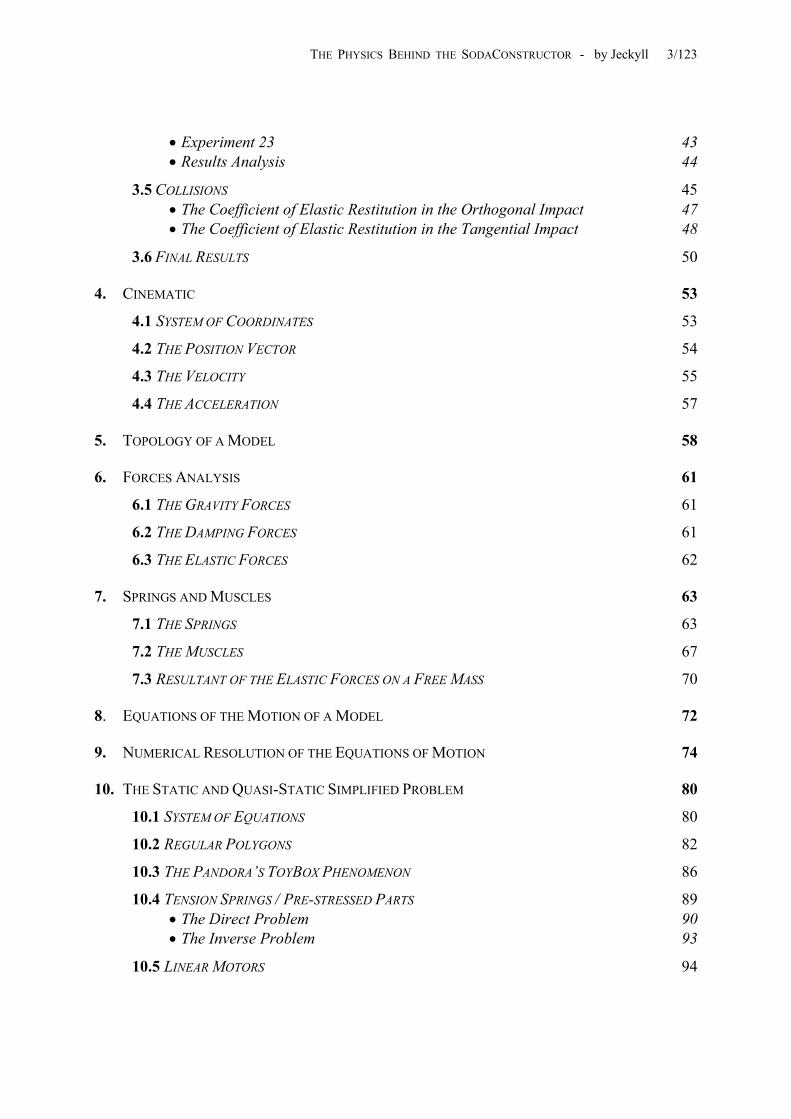
CONTENTS
1. INTRODUCTION 5
2. UNITS OF MEASUREMENT 7
3. DETERMINATION OF THE PHYSICAL CONSTANTS ADOPTED BY THE APPLET 11
3.1 THE GRAVITY 12 • Experiment 1 15 • Experiment 2 16 • Experiment 3 16 • Experiment 4 17 • Experiment 5 17 • Results Analysis 18
3.2 THE STIFFNESS (STATIC METHOD) 20 • The Static Experiments 23 • Experiment 6 24 • Experiment 7 24 • Experiment 8 25 • Results Analysis 26
3.3 THE STIFFNESS (DYNAMIC METHOD) 27 • Experiment 9 28 • Experiment 10 29 • Experiment 11 29 • Experiment 12 30 • Experiment 13 30 • Results Analysis 31
3.4 THE FRICTION 32 • Experiment 14 35 • Experiment 15 36 • Experiment 16 37 • Experiment 17 38 • Experiment 18 39 • Experiment 19 39 • Experiment 20 40 • Experiment 21 41 • Experiment 22 42
THE PHYSICS BEHIND THE SODACONSTRUCTOR - by Jeckyll 3/123
• Experiment 23 43 • Results Analysis 44
3.5 COLLISIONS 45 • The Coefficient of Elastic Restitution in the Orthogonal Impact 47 • The Coefficient of Elastic Restitution in the Tangential Impact 48
3.6 FINAL RESULTS 50
4. CINEMATIC 53
4.1 SYSTEM OF COORDINATES 53
4.2 THE POSITION VECTOR 54
4.3 THE VELOCITY 55
4.4 THE ACCELERATION 57
5. TOPOLOGY OF A MODEL 58
6. FORCES ANALYSIS 61
6.1 THE GRAVITY FORCES 61
6.2 THE DAMPING FORCES 61
6.3 THE ELASTIC FORCES 62
7. SPRINGS AND MUSCLES 63
7.1 THE SPRINGS 63
7.2 THE MUSCLES 67
7.3 RESULTANT OF THE ELASTIC FORCES ON A FREE MASS 70
8. EQUATIONS OF THE MOTION OF A MODEL 72
9. NUMERICAL RESOLUTION OF THE EQUATIONS OF MOTION 74
10. THE STATIC AND QUASI-STATIC SIMPLIFIED PROBLEM 80
10.1 SYSTEM OF EQUATIONS 80
10.2 REGULAR POLYGONS 82
10.3 THE PANDORA’S TOYBOX PHENOMENON 86
10.4 TENSION SPRINGS / PRE-STRESSED PARTS 89 • The Direct Problem 90 • The Inverse Problem 93
10.5 LINEAR MOTORS 94

THE PHYSICS BEHIND THE SODACONSTRUCTOR - by Jeckyll 4/123
11. CONCLUSIONS AND ACKNOWLEDGEMENTS 98
APPENDIX A: THE PENDULUM 99
APPENDIX B: DAMPED FREE VIBRATIONS (SINGLE DEGREE OF FREEDOM) 103 • The Undamped Free Vibrations 112
APPENDIX C: OTHER NUMERICAL TECHNIQUES 114 • The Euler’s Method: Non-Linear Differential Equation of First Order 114 • The Euler’s Method: System of Non-Linear Differential Equations of First Order 117 • The Euler’s Method: Non-Linear Differential Equations of Second Order 118 • The Euler’s Method: Systems of Differential Equations of Second Order 120 • The Euler’s Method: Final Considerations 120 • The Runge-Kutta’s Algorithm 121

THE PHYSICS BEHIND THE SODACONSTRUCTOR - by Jeckyll 5/123
1. INTRODUCTION
The sodaconstructor applet is simply a simulator of the mechanical laws of physics. In
the following chapters of this article, we will investigate these physical laws and the way they
have been implemented in the applet. Here I wish to express just a few preliminary
considerations.
First, I wish to say that in this work you will not find anything really original in the scientific
meaning of the term. Everything reported in this paper is a well-known notion of physics and
mathematics. Therefore, this article can’t be catalogued in the category of scientific work, but
rather in the category of didactical publication. Thanks to this paper, anyone with a minimal
knowledge of the main mathematical rules of analysis can discover with his own hands how
the sodaconstructor applet works.
A second thing that I wish to say here is particularly addressed to anyone who because of his
young age or particular field of study doesn’t totally understand the mathematics in this work.
For you I repeat another time that there is nothing special presented in this work. All these
things, scientifically speaking, are trivial. If you wish to see something really original, then
look for models in the sodazoo. There you will find genuine creativity. Let me use a simple
analogy that I think better explains what I’m trying to say. The sodaconstructor applet is
something like a musical instrument. It isn’t particular important who made a piano; it is more
important who plays the piano! I’m not sure of this, but I would bet money that Mozart and
Beethoven knew nothing about the mechanism behind their own pianos. So, I wish to stress
one thing: please, don’t stop playing the piano.
Finally, I wish to provide here a short description of the contents of this work. This paper is
organized in chapters, further separated, where necessary, into subsections. In the second
chapter particular units of measurement are studied. In the third chapter virtual experiments
are realized in order to investigate the physical constants adopted by the applet. In this chapter
the functionalities of the applet’s cursors of gravity, friction and stiffness are experimentally
determined. All these experiments have been adequately described and the corresponding
links are included in the text of the explanations. In the fourth chapter, the main cinematic
quantities for the description of the motion of free masses are introduced and discussed. In the
fifth chapter, a simple definition of a model is introduced. The sixth chapter gives a detailed

THE PHYSICS BEHIND THE SODACONSTRUCTOR - by Jeckyll 6/123
analysis of the forces implemented in the applet. The seventh chapter provides a detailed
mathematical explanation of the behavior of springs and muscles. In this chapter the
functionalities of the cursors of the muscle control panel are completely clarified. In the
eighth chapter, the equations of motion for a generic model are formulated, while in the ninth
chapter, we find a simple numerical procedure for their integration. In the tenth chapter, a
simplified method for the study of models is introduced. This chapter studies polygons,
tension springs, and linear motors. Finally, the eleventh chapter contains the conclusion and
acknowledgements. The paper is also accompanied by three appendixes, in which specific
mathematical arguments are studied in-depth.
November 2002 Jeckyll

THE PHYSICS BEHIND THE SODACONSTRUCTOR - by Jeckyll 7/123
2. UNITS OF MEASUREMENT
In the real world, especially in scientific and technical communications, all physical
quantities are expressed in units of measurement defined by the International System (S.I.).
We all know that the unit of measurement for length is the meter (m), the unit of measurement
for time is the second (s), the unit of measurement for mass is the kilogram (kg), and so on for
the other fundamental quantities (temperature, intensity of current, etc.). In the soda universe,
however, we can’t use these units of measurement. To illustrate why, let’s explore this
seemingly simple question: how long, for example, is the old charming daintywalker? I have a
17-inch monitor, and I measure a length of 7.9 cm. Is this the right answer? Certainly not.
Another person with a different size monitor would find a different measure. Furthermore, it
is even possible that two different people, each with the same size monitor, would find two
different measures because their monitors are of different brands. It’s clear why it isn’t
adequate to use the meter (and its submultiples) as the unit of measurement for length in the
sodaconstructor: the measurement would be slightly different for each person.
Obviously, in the soda universe it is essential to choose another unit of measurement for
length. Since the amount of pixels in the sodaconstructor window is the same for all users
( : see pxlpxl 428657 × Dimensions of the Sodaconstructor Window), independent of the
dimensions of the monitor screen, in this paper we will use the pixel as the unit of
measurement for length. The symbol that we will adopt will be: pxl. The main problem with
this new unit of measurement is this: how is it possible to measure something in pixels
without counting all the pixels one by one? This is not a trivial question, because to count
many pixels on the screen is excruciatingly painful. Therefore, I’ve used the following
technique: I know that a fixed mass (I really don’t like this denomination, I would have
preferred fixed point) has the following dimensions: 6 . So, by arranging many
fixed masses like a chessboard, it is possible to measure the distance between two different
points on the screen by simply counting the fixed masses between the two points and
multiplying the amount by 6. Obviously, it is possible that the length we want to measure is
not a multiple of 6; in this case we will arrange the fixed masses like a chessboard until we
are less than 6 pixels from the endpoint, and we will count the remaining pixels, 5 at the most.
Sometimes, however, the length that we want to measure is so great that the above fixed
masses method would be equally painful for our eyes and patience. In this case it is possible
pxlpxl 6×

THE PHYSICS BEHIND THE SODACONSTRUCTOR - by Jeckyll 8/123
to apply a mixed method, such as using fixed masses to measure distances greater than 6
pixels. One of my favorite ways to get equal distances between fixed points is by constructing
springs at 0°, 45° and 90°, angles which are easy to precisely create in the sodaconstructor.
Using these lines to make perfect squares, it is easy to replicate a fixed length many times, in
order to measure using larger increments. I’ve used this technique often, as you will see in
examples referred to later (you will find one example in Dimensions of the Sodaconstructor
Window).
Another physical quantity involved in these studies is time. Again, it is impossible to use the
usual unit of measurement (seconds s). In principle it should be possible to use the second (s)
as a measurement of time, because advanced simulation programs like our beloved
Sodaconstructor should synchronize their calculus with the internal microprocessor clock. For
this reason, the duration of the simulation should be uniform in all different computers.
However, all computers are different from each other. Computers today are assembled with
many different parts: there are the microprocessors, the main boards, the accelerated graphic
devices, and many other such devilries. (Are there any of you young people old enough to
remember the simplicity of the Commodore 64? I bet you don’t.) The real performance of a
computer depends greatly on all its different components. Therefore, it is very difficult to find
two different computers with identical performances. For these reasons, I suspect that the
same simulation could have different durations on different computers. It may seem that I am
being unnecessarily precise. Nevertheless, as you will see in the next chapter, I will need
maximum precision to get reliable results.
Just as with pixels, the number of frames necessary to complete a simulation is exactly the
same for each computer. So, to avoid any ambiguity, we will use the frame as our unit of
measurement for time. The symbol that we will adopt will be: frm. Now the problem is: how
can we count the amount of frames that it takes for a particular model to complete a
simulation? The surprising answer is: using an ordinary chronometer. This seems like a
contradiction, but it isn’t. The main problem is that in the sodaconstructor applet there isn’t a
frame counter, so the only thing that we can use is a chronometer. Using the new sodarace
timetrial applet, each of us can find how many frames there are in a second for our own
computer’s performance. Those of us with a computer of high performance will get many
frames in a second. Those of us with a computer of less power will not get as many frames in

THE PHYSICS BEHIND THE SODACONSTRUCTOR - by Jeckyll 9/123
a second. Thanks to the synchronicity between the simulator’s computation and the internal
clock of the computer, the difference between two different computers will probably never be
very high. Still, I think there will always be a difference. In any case, if each of us finds for
his own computer how many frames there are in a second, it solves the problem. After this
has been determined, the length in frames of a particular simulation can be calculated by
multiplying the number of seconds by the number of frames per second. The result in frames
should be the same for everyone, completely independent of the computer’s performance.
The last question is: how can I find how many frames there are in a second of my computer’s
work? This can be determined using any model in the sodarace timetrial. In order to make this
as accurate as possible, I made a very slow model (Slow walker). In my computer it covered
the whole route in 966 (1 : an eternity) for a total of 107036 . So, the time
conversion ratio ( t ) for my computer is:
sec 606 ′′′ frm
cr
secfrmtcr 81.110
966107036
== (2.1)
This ratio is very important because I use it in the virtual experiences described in the next
chapter.
To review, we will be using the following units of measurement:
Table 2.1: The new units of measurement
Physical quantity Unit of measurement
Length pxl (pixel)
Time frm (frame)
Velocity frmpxl
Acceleration 2frmpxl
What about mass? We know that the other fundamental physical quantity involved in the
dynamic problem is mass. Well, in the 8th chapter I will show you mathematically that it isn’t

THE PHYSICS BEHIND THE SODACONSTRUCTOR - by Jeckyll 10/123
necessary to assume any value for the masses. This is because all masses in the
sodaconstructor applet are the same.

THE PHYSICS BEHIND THE SODACONSTRUCTOR - by Jeckyll 11/123
3. DETERMINATION OF THE PHYSICAL CONSTANTS ADOPTED BY THE APPLET
As we all know, there are many constants present in the physical laws that govern our
world. One of the most important constants, one that often persecutes students in school, is
the earth’s gravitational acceleration constant g. In the proximity of the Earth’s surface, the
value of this constant is about 28.9 secmg = . Thanks to the knowledge of this constant, we
can say many things. First, we can say that the velocity of a free falling body close to the
Earth’s surface increases secm8.9 every second of its falling (this is true only until air
friction begins to have an effect; i.e. just in the first few seconds of its falling). Another thing
that this constant allows us to say it is that the weight W (expressed in Newton N) of a generic
mass m (expressed in kg) is obtained by the rule:
(3.1) gmW ⋅=
These apparently simple things allow us to see how the knowledge of the constant g is,
without a doubt, very important for a lot of physical and engineering applications. Obviously,
in addition to the constant g, there are a lot of other constants that are equally important. All
these constants have specific values commonly known by the scientific community. The
question is: how were these constants originally found? The answer is very simple: by means
of experimental tests.
How does all this relate to the sodaconstructor? To answer this question we must first
understand exactly what the sodaconstructor is. The sodaconstructor is simply a simulator of
physical laws. In the sodaconstructor there are a number of mechanical laws1 that, like in
reality, cannot be violated. Therefore, in principle, it should be possible to determine the
physical constants of the laws used in the sodaconstructor by means of virtual experiments,
much like the experimental tests that allow us to understand nature in the real world.
Of course, if I were an expert in computer languages I would simply find the
sodaconstructor’s physical constants by looking for them in the soda algorithm.
Unfortunately, I am not an expert. So the best thing that I can do is transform myself into a
1 The Newtonian laws of dynamics, Hooke’s law for the springs, the Newtonian law for the fluid’s friction, the laws of the quasi-elastic impact between masses and walls.

THE PHYSICS BEHIND THE SODACONSTRUCTOR - by Jeckyll 12/123
virtual Galileo (Italian scientist of the seventeenth century) in order to investigate the soda
universe.
I’ve created a sodaconstructor Laboratory where I’ve executed many virtual experiments.
Thanks to these experiments I was able to find how the well-known cursors for gravity (g),
friction (f) and stiffness (k) actually work (see Fig. 3.1).
Figure 3.1: The physical sodaconstructor constants
In the following parts of this chapter I will explain exactly what I’ve determined about each
one of the above constants. I’ve also investigated about the coefficients of dynamical
restitutions of the walls and ground.
3.1 THE GRAVITY
In the real universe we could think of a simple experimental test to determine the
gravitational acceleration constant g. We could let a little object like a stone fall from a fixed
height h. Meanwhile we could measure the time t it takes the stone to fall by means of a
chronometer. Knowing that the falling stone moves with a uniformly accelerated motion, we
could use the following formula:
221 gth = (3.2)
to get the acceleration g:
2
2thg = (3.3)

THE PHYSICS BEHIND THE SODACONSTRUCTOR - by Jeckyll 13/123
In fact, this method of determining the constant g isn’t very accurate, because air friction will
have an effect. A more accurate method of determining the constant g is the pendulum
method. It is possible to find the constant g by simply measuring the period of a complete
oscillation of a long pendulum2.
What can we do in the soda universe? Exactly the same things! We could get the acceleration
constant3 g by using the experiment of a mass falling. Fortunately, in the soda universe we
have the option to turn off the “air” friction completely, so we don’t need to worry about the
problem described above. Still, this method is a bit problematic. First, I don’t have an
accurate chronometer; I just measure time with my analog clock, which means I only have the
accuracy of one second (an eternity compared to the accuracy required in this sort of
experiment). Second, it is very difficult to start the chronometer exactly when the mass begins
falling. Third, it is also very difficult to stop the chronometer exactly when the mass hits the
ground. As a result, I would get a measure with an intolerable error. What could I do to fix
this problem? I could conduct this experiment a number of times, so that I could reduce the
margin of error. But this method it is too long and tedious, even for my patience. However,
there is a more convenient and accurate solution: to use the pendulum method. Using as long
a pendulum as possible and measuring its period2, we can discover the gravitational
acceleration constant g.
In Appendix A, I will explain in a detailed manner the mathematical theory behind the
pendulum method. Therefore, in the following description, I will restrict myself to explaining
only the main relation that we will use.
As discussed in Appendix A, when the maximum angular excursion (expressed in
radiant rad) of a pendulum is such that it is possible to use the following approximation:
maxα
(3.4) maxmaxsin α≈α
2 The time that the pendulum needs to reach its maximum excursion starting from the identical position. 3 There is a point I want to make clear about the word “constant” in the soda universe. As we well know it is possible to change the gravity by moving the above mentioned gravity cursor. Therefore, in principle, the gravity isn’t constant. Nevertheless, if we choose a particular level of gravity, our models are moving with a value of gravity that doesn’t change over time; in this case the gravity is constant.

THE PHYSICS BEHIND THE SODACONSTRUCTOR - by Jeckyll 14/123
(just when the value of is very small; see Fig. 3.2) the period T of an oscillation
depends only on the length l of the pendulum and the gravity constant g, by means of the
formula:
maxα
glT π= 2 (3.5)
maxα maxα
l
α
Figure 3.2: Angular excursion of a pendulum
By measuring the period T and knowing the length of the pendulum it is possible to get the
constant g by means of the following inverse formula:
2
24Tlg π= (3.6)
Some might argue that this unnecessarily complicated, because to measure the period T I will
have the same difficulties as described for the falling mass method. This isn’t true! If friction
is dropped to zero, the pendulum’s oscillation could last forever. Therefore, it will be possible
to measure not just one complete oscillation but many oscillations. In this way the inevitable
errors mentioned above will be distributed in many oscillations, reducing their effect on the
final computation. This is exactly what I’ve done. Fixing a particular value for the gravity by

THE PHYSICS BEHIND THE SODACONSTRUCTOR - by Jeckyll 15/123
moving the well-known cursor4, I measured the elapsed time for many oscillations. Then, I
divided the overall time by the number of complete oscillations, giving me the period T of a
single oscillation with the required accuracy.
Before I start explaining the virtual experiences about gravity, I will say just one thing about
the cursors shown in Figure 3.1. Each one of these cursors can assume 108 different positions.
Each of these 108 positions differs from the previous or the following position by one pixel of
displacement. We have position 0 when the cursor is at the bottom (in this position the
physical quantity associated with the cursor has the value of zero), and we have position 107
when the cursor is at the top (in this position the physical quantity associated with the cursor
has the maximum value).
In the following section we will look for the rules of variation for the constants g, f, and k in
respect to their cursor position. So, naming these positions , and , we will look for
the following three laws:
gp fp kp
( )( )( )
107,,2,1,0,with , K=
kfg
k
f
g
ppppkpfpg
(3.7)
• Experiment 1
Using Experiment 1 it was possible to find the value of the gravitational acceleration
constant g (in 2frmpxl ) when the gravity cursor position is . The length of the
pendulum in this case is l .
20=gp
pxl374=
I measured the time it took for 100 complete oscillations. On my computer this time was
( 3 ), so the period of a single oscillation was: sect 293= 54 ′′′
secT 93.2100293
==
By using the time conversion ratio (2.1) the period T becomes:
4 I’ve also dropped the friction to zero and taken at the maximum value the rigidity of the spring that connects the free mass at the fixed point. In the pendulum theory the connection between the mass and the fixed point should be perfectly rigid.

THE PHYSICS BEHIND THE SODACONSTRUCTOR - by Jeckyll 16/123
frmsecfrmsecT 67.32481.11093.2 =⋅=
Applying (3.6) I finally found:
( )2
140067762.020frmpxlg =
For now we will ignore the question of significant digits. We will discuss this at the end of the
chapter.
• Experiment 2
Using Experiment 2 it was possible to find the value of the gravitational acceleration
constant g (in 2frmpxl
pxl374=
) when the cursor position is . The length of the pendulum
in this case is l .
29=gp
I measured the time it took for 100 complete oscillations. On my computer this time was
( ), so the period of a single oscillation was: sect 202= 223 ′′′
secT 02.2100202
==
By using the time conversion ratio (2.1) the period T becomes:
frmsecfrmsecT 84.22381.11002.2 =⋅=
Applying (3.6) I finally found:
( )2
294693591.029frmpxlg =
• Experiment 3
Using Experiment 3 it was possible to find the value of the gravitational acceleration
constant g (in 2frmpxl
pxl375=
) when the cursor position is . The length of the pendulum
in this case is l .
40=gp
I measured the time it took for 150 complete oscillations. On my computer this time was
( 0 ), so the period of a single oscillation was: sect 220= 43 ′′′

THE PHYSICS BEHIND THE SODACONSTRUCTOR - by Jeckyll 17/123
secT 47.1150220
==
By using the time conversion ratio (2.1) the period T becomes:
frmsecfrmsecT 52.16281.11047.1 =⋅=
Applying (3.6) I finally found:
( )2
560493075.040frmpxlg =
• Experiment 4
Using Experiment 4 it was possible to find the value of the gravitational acceleration
constant g (in 2frmpxl
pxl375=
) when the cursor position is . The length of the pendulum
in this case is l .
50=gp
I measured the time it took for 150 complete oscillations. On my computer this time was
( 6 ), so the period of a single oscillation was: sect 176= 52 ′′′
secT 17.1150176
==
By using the time conversion ratio (2.1) the period T becomes:
frmsecfrmsecT 02.13081.11017.1 =⋅=
Applying (3.6) I finally found:
( )2
875770431.050frmpxlg =
• Experiment 5
Using Experiment 5 was possible to get the value of the gravitational acceleration
constant g (in 2frmpxl
pxl376=
) when the cursor position is . The length of the pendulum
in this case is l .
60=gp
I measured the time it took for 200 complete oscillations. On my computer this time was
( 6 ), so the period of a single oscillation was: sect 196= 13 ′′′

THE PHYSICS BEHIND THE SODACONSTRUCTOR - by Jeckyll 18/123
secT 98.0200196
==
By using the time conversion ratio (2.1) the period T becomes:
frmsecfrmsecT 59.10881.11098.0 =⋅=
Applying (3.6) I finally found:
( )2
25874431.160frmpxlg =
• Results Analysis
Displaying the above results in a graph in which the horizontal axis represents the cursor
position and the vertical axis represents the gravitational acceleration constant g, we get
the curve of Figure 3.3:
gp
2frm
pxlg
gp 10 20 30 40 50 60
0.2
0.4
0.6
0.8
1
1.2
Figure 3.3: gravity trend
Looking the curve of Figure 3.3 we can immediately see that the relation between g and
is not linear. Since the curve looks more similar to a parabola, we can try to calculate the ratio
between g and . The following table shows the result of this calculation for all the above
experiences:
gp
2gp

THE PHYSICS BEHIND THE SODACONSTRUCTOR - by Jeckyll 19/123
Table 3.1: Ratio 2gpg for the above experiences
gp
2frm
pxlg 2gp
g
20 0.140067762 0.000350169
29 0.294693591 0.000350409
40 0.560493075 0.000350308
50 0.875770431 0.000350308
60 1.25874431 0.000349651
Since the ratio 2gpg is practically constant for all 5 of the above virtual experiences, we can
affirm that between g and there is a quadratic proportionality: gp
( )
⋅=
22
frmpxlpgpg gPg (3.8)
In the formula above I’ve introduced the gravity parameter which is a constant parameter
implemented in the sodaconstructor applet. If I were extremely precise I would find the
gravity parameter by means of a quadratic interpolation of the above data, but
remembering that all of this is just play, I will restrict myself to the calculation of the medium
value of . From Table 3.1 we can find the following medium value for :
pg
pg
pg pg
⋅=
22000350169.0
gp
pfrmpxlg (3.9)
Figure 3.4 displays the numerical data of Table 3.1 and the continuous curve made from (3.8)
and (3.9). As can clearly be seen, in the range of that was used in the experiments
( ) there is a perfect overlapping.
gp
[ 60,20∈gp ]

THE PHYSICS BEHIND THE SODACONSTRUCTOR - by Jeckyll 20/123
2frm
pxlg
gp 10 20 30 40 50 60
0.2
0.4
0.6
0.8
1
1.2
Figure 3.4: Overlapping between numerical data and theoretical curve
3.2 THE STIFFNESS (STATIC METHOD)
The main components of the sodaconstructor are springs and muscles. These components
have elastic properties that are defined by a physical quantity called stiffness. To understand
what the elastic properties of springs exactly are and how these properties are represented by
stiffness, we could make some observations of springs in the real world. We all know what
real springs are and what characteristics they possess. We know, for example, that a spring
changes length only when force is applied to its ends, and that when this force stops the spring
returns to its original length. We also know that the force necessary to pull a spring increases
with the spring’s extension. Finally, we know that two springs of different strengths subjected
to the same forces have different extensions.
These observations show the basic concepts of elasticity and stiffness. We will say that a body
is an elastic body if its deformations vanish when their causes are removed. We will say that a
body is a linear elastic body if its deformations are directly proportional to the forces applied
to the body. Finally we will define stiffness as how well an elastic body can maintain its
original shape (or length if we are specifically speaking of a spring) when it is subjected to
external forces.
For springs, all these characteristics can be mathematically defined in a very simple way.

THE PHYSICS BEHIND THE SODACONSTRUCTOR - by Jeckyll 21/123
F
l 0l
Figure 3.5: Extension of a spring subjected to traction by a force F
Figure 3.5 shows a spring before and after the action of a traction force F. Calling the
length of the spring at rest and l the length of the spring after extended, we will define the
quantity of the spring’s extension:
0l
(3.10) 0lll −=∆
By definition, the extension of a spring will be positive if its final length l is greater than the
initial length . The extension of a spring will be negative if its final length l is less than the
initial length .
0l
0l
If the spring is a linear elastic spring (like the springs in the sodaconstructor applet), then the
spring’s extension will be directly proportional to the force’s intensity F by means of the
relation:
l∆
(3.11) lkF ∆⋅=
This law is known as Hooke’s law5. The constant k that appears in (3.11) is the stiffness of the
spring and is a physical quantity that is always positive. Its value is representative of the
spring’s strength. Using (3.11), we can say:
5 Robert Hooke was an English scientist of seventeenth century, contemporaneous of Isaac Newton. It seems that the two scientists weren’t particularly fond of each other. It is ironic that in our beloved sodaconstructor applet their laws live together harmoniously.

THE PHYSICS BEHIND THE SODACONSTRUCTOR - by Jeckyll 22/123
kFl =∆ (3.12)
It is easy to understand that under the same force, springs with high values of stiffness k will
have extensions smaller than those of springs with low stiffness.
From (3.11) we can also see that if the force is positive, its effect on the spring will be
positive (extension), while if the force is negative, its effect on the spring will be negative
(compression).
The stiffness k that appears in (3.11) and (3.12) is the same physical quantity that can be
changed with the cursor k (see Fig. 3.1) in the sodaconstructor applet. There is one more thing
I must emphasize about the sodaconstructor’s virtual springs: all springs, regardless of their
initial length, have the same stiffness6. In the current version of the applet it is impossible to
have springs of independent stiffness in the same simulation.
By means of static virtual experiments, the expression (3.11) will allow us to determine the
value of the stiffness k depending on the position of the corresponding cursor. Obviously, in
order to use (3.11) to find the stiffness k, we will need a static force F. But how can we create
a static force? We can simply use the force of gravity. We know that a mass m in a constant
gravitational field has a weight given by the expression (3.1). Therefore, in order to create a
constant force in our experiments, we will use the virtual weight of free masses in the
sodaconstructor applet.
It might be important at this point to say something about the sodaconstructor’s free masses.
By means of very simple virtual experiments it is possible to prove that all free masses are
equal7, so we will have just one value of mass m for all free masses. At the moment, we will
leave this value unknown. In the Chapter 8 we will see why it is possible to avoid having to
assume any specific value for m.
6 i.e. all springs, regardless of their initial length, will be subject to the same extension under the same force. 7 I will leave to you the pleasure of devising some simple experiments.

THE PHYSICS BEHIND THE SODACONSTRUCTOR - by Jeckyll 23/123
• The Static Experiments
Just as we did with the gravity g, our objective will be to find how the spring’s stiffness k
changes according to the position of the corresponding cursor; i.e. our objective will be to
discover the law:
(3.13) ( kpkk = )
In order to find this law we will apply the weight of a free mass to springs of different
lengths8, using different fixed values of stiffness. Therefore, the constant force F in the
relation (3.11) for us will be the weight W of a free mass given by (3.1). Then we will have:
(3.14) lkgmWF ∆⋅=⋅==
so that:
ml
gk ⋅∆
= (3.15)
In (3.15), we know the value of g thanks to (3.8) and (3.9), and we will find the extension
by measuring it. As I’ve said before, at the moment we will leave the value of m unknown, so
it will be helpful to define the following physical quantity:
l∆
l
gmkk
∆== (3.16)
which is independent of the value of m. We will call k specific stiffness.
Thanks to the introduction of specific stiffness we can write (3.15) as:
mkk ⋅= (3.17) 8 I’ve used springs of different lengths to prove without any doubt that the stiffness of a spring is absolutely independent of its initial length.

THE PHYSICS BEHIND THE SODACONSTRUCTOR - by Jeckyll 24/123
• Experiment 6
In Experiment 6 the extensions of springs of different lengths have been measured with
the stiffness cursor position equal to . The force F has been varied by changing the
position of the gravity cursor from to by increments of 10. For each setting
of gravity, the extension of the springs has been measured and the results reported in the
following Table 3.2:
20=kp
30=gp 100=gp
Table 3.2: Spring’s extension for different values of gravity when 20=kp
gp
2frm
pxlg [ ]pxll∆
∆ 21
frmlg
30 0.3151521 18 0.01750845
40 0.5602704 32 0.01750845
50 0.8754225 50 0.01750845
60 1.2606084 72 0.01750845
70 1.7158281 98 0.01750845
80 2.2410816 128 0.01750845
90 2.8363689 162 0.01750845
100 3.50169 200 0.01750845
Using the above results, we find the average value of the specific stiffness for the cursor
position : 20=kp
( )2
101750845.020frm
k = (3.18)
• Experiment 7
In Experiment 7 the extensions of springs of different lengths have been measured with
the stiffness cursor position equal to . The force F has been varied by changing the 25=kp

THE PHYSICS BEHIND THE SODACONSTRUCTOR - by Jeckyll 25/123
position of the gravity cursor from to by increments of 10. For each setting
of gravity, the extension of the springs has been measured and the results reported in the
following Table 3.3:
30=gp 100=gp
2frm
pxl [ ]pxll∆
Table 3.3: Spring’s extension for different values of gravity when 25=kp
gp g ∆
2
1frml
g
30 0.3151521 11 0.028650191
40 0.5602704 20 0.028013520
50 0.8754225 32 0.027356953
60 1.2606084 46 0.027404530
70 1.7158281 62 0.027674647
80 2.2410816 81 0.027667674
90 2.8363689 103 0.027537562
100 3.50169 128 0.027356953
Using the above results, we find the average value of the specific stiffness for the cursor
position : 25=kp
( )2
1027707754.025frm
k = (3.19)
• Experiment 8
In Experiment 8 the extensions of springs of different lengths have been measured with
the stiffness cursor position equal to . The force F has been varied by changing the
position of the gravity cursor from to by increments of 10. For each setting
of gravity, the extension of the springs has been measured and the results reported in the
following Table 3.4:
30=kp
30=gp 100=gp

THE PHYSICS BEHIND THE SODACONSTRUCTOR - by Jeckyll 26/123
Table 3.4: Spring’s extension for different values of gravity when 30=kp
gp
2frm
pxlg [ ]pxll∆
∆ 21
frmlg
30 0.3151521 8 0.039394013
40 0.5602704 14 0.040019314
50 0.8754225 22 0.039791932
60 1.2606084 32 0.039394013
70 1.7158281 43 0.039902979
80 2.2410816 56 0.040019314
90 2.8363689 72 0.039394013
100 3.50169 88 0.039791932
Using the above results, we find the average value of the specific stiffness for the cursor
position : 30=kp
( )2
1039713439.030frm
k = (3.20)
• Results Analysis
In this case we have the values of the specific stiffness for only three positions on the
cursor , so it will be impossible to get as good a curve as we did with the gravity
experiments. Therefore we will limit ourselves to a simple analysis of the above numerical
data. Based on the results of our gravity experiments, it is reasonable to guess that the
relationship between the specific stiffness and is once again quadratic. In order to verify
this hypothesis we will calculate the ratio
kp
kp
( ) 2kpk pk for each of the three results reported in
(3.18), (3.19) and (3.20).

THE PHYSICS BEHIND THE SODACONSTRUCTOR - by Jeckyll 27/123
Table 3.5: Ratio 2kpg for the above experiments
kp
2
1frm
k
22
1frmp
k
k
20 0.01750845 0.000043771
25 0.027707754 0.000044332
30 0.039713439 0.000044126
Because the results of the ratio ( ) 2kk ppk are approximately constant, we can assume with
very little doubt the following rule for specific stiffness:
( ) 2kpk pkpk ⋅= (3.21)
in which has been introduced the parameter pk that we will call the stiffness parameter. Just
as with the gravity parameter , the stiffness parameter pg pk is a constant parameter
implemented in the sodaconstructor applet. Its medium value is (see Table 3.5):
=
21000044077.0
frmk p (3.22)
Therefore the rule for the stiffness k, thanks to (3.17) and (3.21), will be:
( ) ( ) 2kpkk pmkmpkpk ⋅⋅=⋅= (3.23)
3.3 THE STIFFNESS (DYNAMIC METHOD)
There is another and more accurate method of determining the stiffness of a spring. This
method is very similar to the dynamic method that we used for the gravity experiments. By
simply measuring the period of the oscillation of a spring connected to one mass, it is possible
to calculate the spring’s stiffness. In the following section I will restrict myself to explain just

THE PHYSICS BEHIND THE SODACONSTRUCTOR - by Jeckyll 28/123
the main relation that we will use. A more detailed explanation of this method can be found in
Appendix B.
k m
Figure 3.6: System spring-mass
Calling k, m and T respectively the stiffness of a spring, the value of the mass connected with
the spring and the period of a complete oscillation of the system spring-mass (see Fig. 3.6), it
is possible to show that the following relation is valid:
mT
k2
24π= (3.24)
Using this relation, it is possible to get the stiffness of a spring by measuring the period T.
Taking into account (3.17), from (3.24) follows immediately the expression for the specific
stiffness k :
2
24T
k π= (3.25)
Obviously, like in the gravity determination, with friction equal to zero the oscillations of the
spring will last forever. Therefore, to get a more accurate reading, we will measure the
duration of more than one oscillation.
• Experiment 9
In Experiment 9, it was possible to find the value of the specific stiffness k (in 2frm1 )
when the cursor position was . The duration of 100 complete oscillations has been 6=kp
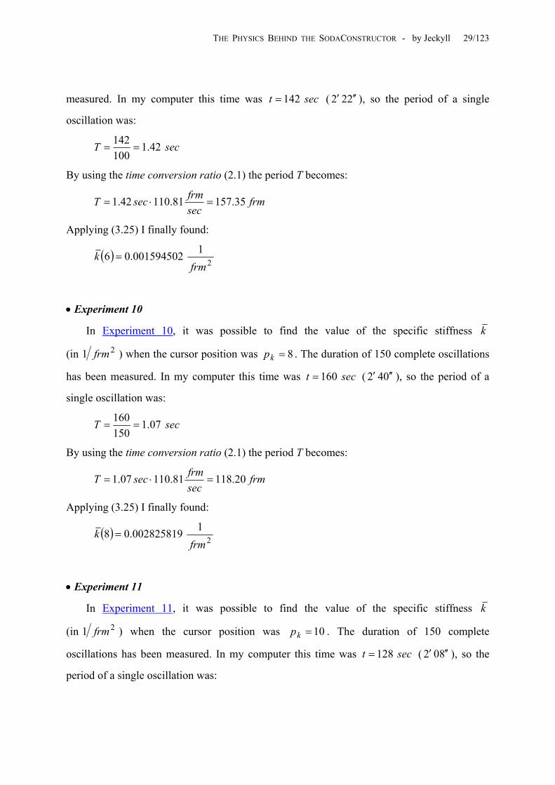
THE PHYSICS BEHIND THE SODACONSTRUCTOR - by Jeckyll 29/123
measured. In my computer this time was ( 22 ), so the period of a single
oscillation was:
sect 142= 2 ′′′
8=kp
= sec160
10=kp
secT 42.1100142
==
By using the time conversion ratio (2.1) the period T becomes:
frmsecfrmsecT 35.15781.11042.1 =⋅=
Applying (3.25) I finally found:
( )2
1001594502.06frm
k =
• Experiment 10
In Experiment 10, it was possible to find the value of the specific stiffness k
(in 2frm1 ) when the cursor position was . The duration of 150 complete oscillations
has been measured. In my computer this time was t ( 02 ), so the period of a
single oscillation was:
4 ′′′
secT 07.1150160
==
By using the time conversion ratio (2.1) the period T becomes:
frmsecfrmsecT 20.11881.11007.1 =⋅=
Applying (3.25) I finally found:
( )2
1002825819.08frm
k =
• Experiment 11
In Experiment 11, it was possible to find the value of the specific stiffness k
(in 2frm1 ) when the cursor position was . The duration of 150 complete
oscillations has been measured. In my computer this time was ( 2 ), so the
period of a single oscillation was:
sect 128= 80 ′′′

THE PHYSICS BEHIND THE SODACONSTRUCTOR - by Jeckyll 30/123
secT 85.0150128
==
By using the time conversion ratio (2.1) the period T becomes:
frmsecfrmsecT 56.9481.11085.0 =⋅=
Applying (3.25) I finally found:
( )2
1004415343.010frm
k =
• Experiment 12
In Experiment 12, it was possible to find the value of the specific stiffness k
(in 2frm1 ) when the cursor position was . The duration of 150 complete
oscillations has been measured. In my computer this time was t ( 71 ), so the
period of a single oscillation was:
12=kp
sec107= 4 ′′′
secT 71.0150107
==
By using the time conversion ratio (2.1) the period T becomes:
frmsecfrmsecT 04.7981.11071.0 =⋅=
Applying (3.25) I finally found:
( )2
1006318541.012frm
k =
• Experiment 13
In Experiment 13, it was possible to find the value of the specific stiffness k
(in 2frm1 ) when the cursor position was . The duration of 150 complete
oscillations has been measured. In my computer this time was t (1 ) so the
period of a single oscillation was:
14=kp
sec91= 13 ′′′
secT 61.015091
==

THE PHYSICS BEHIND THE SODACONSTRUCTOR - by Jeckyll 31/123
By using the time conversion ratio (2.1) the period T becomes:
frmsecfrmsecT 22.6781.11061.0 =⋅=
Applying (3.25) I finally found:
( )2
1008735777.014frm
k =
• Results Analysis
Displaying the above results in a diagram in which the horizontal axis represents the
cursor position and the vertical axis represents the specific stiffness kp k , we get the curve
in Figure 3.7:
kp
2
1frm
k
2 4 6 8 10 12 14
0.002
0.004
0.006
0.008
Figure 3.7: specific stiffness trend
First of all, it is possible to see how the curve in Figure 3.7 confirms that there isn’t a direct
proportionality between k and . Therefore, also taking into account the result obtained in
the previous section 3.2, we will try to calculate the ratio between
kp
k and for the above
results. If there were no errors in the experiments or calculations, then the value for the ratio
2kp
2kpk can’t be much different than the value obtained in (3.22). The results of this ratio for
all the above experiments is shown in the following table:

THE PHYSICS BEHIND THE SODACONSTRUCTOR - by Jeckyll 32/123
Table 3.6: Ratio 2kpk for the above experiments
kp
2
1frm
k
22
1frmp
k
k
6 0.001594502 0.000044292
8 0.002825819 0.000044153
10 0.004415343 0.000044153
12 0.006318541 0.000043879
14 0.008735777 0.000044570
Since the ratio 2kpk is practically constant for all five of the above virtual experiments, we
have further evidence of the validity of the experimental relation (3.21). Moreover, it is
possible to see that all the values of the ratio 2kpk are practically the same of the value (3.22)
obtained by means of the static experiments. Since the dynamic experiment gives more
accurate results, for the stiffness parameter we will take the following medium value:
=
21000044209.0
frmk p (3.26)
The quasi-perfect coincidence between the values of pk obtained by means of two different
methods of experiments is proof of the validity of this section of virtual experiments.
3.4 THE FRICTION
The friction discussed here is the friction that a body meets while in movement in a fluid.
Therefore, this kind of friction is related to the viscosity of the medium in which the body is
moving. This friction has essentially two characteristics: the first is that the force of the
friction is always proportional to the body’s velocity; the second is that the force of the
friction is such that its effect is always in opposition of the movement. In order to
mathematically define this kind of friction we will introduce a new physical quantity that in
THE PHYSICS BEHIND THE SODACONSTRUCTOR - by Jeckyll 33/123
the following parts of this paper will be called the damping constant9 and that will be
indicated with the letter f. It is this quantity that we frequently change in our models by
adjusting the second cursor of Figure 3.1.
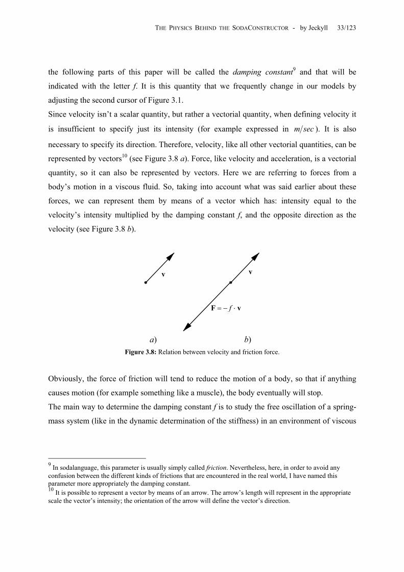
Since velocity isn’t a scalar quantity, but rather a vectorial quantity, when defining velocity it
is insufficient to specify just its intensity (for example expressed in secm ). It is also
necessary to specify its direction. Therefore, velocity, like all other vectorial quantities, can be
represented by vectors10 (see Figure 3.8 a). Force, like velocity and acceleration, is a vectorial
quantity, so it can also be represented by vectors. Here we are referring to forces from a
body’s motion in a viscous fluid. So, taking into account what was said earlier about these
forces, we can represent them by means of a vector which has: intensity equal to the
velocity’s intensity multiplied by the damping constant f, and the opposite direction as the
velocity (see Figure 3.8 b).
vF ⋅−= f
v v
a) b)
Figure 3.8: Relation between velocity and friction force.
Obviously, the force of friction will tend to reduce the motion of a body, so that if anything
causes motion (for example something like a muscle), the body eventually will stop.
The main way to determine the damping constant f is to study the free oscillation of a spring-
mass system (like in the dynamic determination of the stiffness) in an environment of viscous
9 In sodalanguage, this parameter is usually simply called friction. Nevertheless, here, in order to avoid any confusion between the different kinds of frictions that are encountered in the real world, I have named this parameter more appropriately the damping constant. 10 It is possible to represent a vector by means of an arrow. The arrow’s length will represent in the appropriate scale the vector’s intensity; the orientation of the arrow will define the vector’s direction.

THE PHYSICS BEHIND THE SODACONSTRUCTOR - by Jeckyll 34/123
friction: the damped free vibration. A detailed explanation of this method can be found in
Appendix B, so for now, we will just discuss the main relations that will be used.
Leaving a spring-mass system like the one represented in Figure 3.6 free to oscillate in
presence of viscous friction, and calling the mass displacement in respect to the quiet
position at the generic instant t, it is possible to report in a Cartesian diagram the evolution of
the system. By reporting the mass displacement x in the vertical axis and the time t in the
horizontal axis, as we will see in Appendix B, will yield a graphic similar to the following
Figure 3.9.
( )tx
ν+nx nx
•
•
( )tx
t
Figure 3.9: Effect of viscous damping on a free vibration.
Considering two positive peaks between a number of complete cycles of oscillations and
calling and their respective values it is possible to calculate the following
logarithmic parameter
ν
nx ν+nx11:
=δ
ν+n
n
xx
ln (3.27)
Using this, it is possible to get the damping constant f value:
11 We are considering the natural logarithm; i.e. the inverse function of the exponential function e .x

THE PHYSICS BEHIND THE SODACONSTRUCTOR - by Jeckyll 35/123
221
2
δνπ
+
=mk
f (3.28)
In (3.28) we have respectively indicated by k and m the spring’s stiffness and the mass value.
Therefore, taking into account the position (3.17) about the specific stiffness of a spring, we
can rewrite the relation (3.28) as:
mkf221
2
δνπ
+
= (3.29)
Just as with stiffness, it is possible here to introduce a new parameter that we will call specific
damping constant f which doesn’t need the free mass value m:
δνπ
+
=
⋅=
221
2 kf
mff
(3.30)
Thanks to the second formula of (3.30) we will be able to find the sodaconstructor’s law of
variation with the friction cursor’s position of the specific damping fp f .
• Experiment 14
In Experiment 14, it was possible to find the value of the specific damping f (expressed
in frm1 ) when the cursor positions for friction and stiffness were and
respectively. The value of the specific damping
1=fp 6=kp
f should be independent of the stiffness, but
in order to verify this independence, we will repeat every experiment (i.e. for a fixed value of
the cursor position ) with two different values of the specific stiffness. fp

THE PHYSICS BEHIND THE SODACONSTRUCTOR - by Jeckyll 36/123
The peak values of the first and 73rd cycles of oscillations were measured, and the following
values were obtained:
====
=ν=ν+
=
ν+ pxlxxpxlxx
nn
n
n
177291
7273
1
73
1
From (3.27) it follows:
497173535.0177291ln =
=δ
Moreover, using the relations (3.21) and (3.26) in order to get the value of the specific
stiffness, it follows:
( )2
2 1001591524.06000044209.06frm
k =⋅=
Finally, taking into account the previous values, from the 2nd formula (3.30) it follows:
( )frm
f 1000087686.0
497173535.07221
001591524.0212=
π⋅⋅
+
=
• Experiment 15
In Experiment 15, it was possible to find the value of the specific damping f (expressed
in frm1 ) when the cursor positions for friction and stiffness were and
respectively.
1=fp 8=kp
The peak values of the first and 101st cycles of oscillations were measured, and the following
values were obtained:
====
=ν=ν+
=
ν+ pxlxxpxlxx
nn
n
n
173290
100101
1
101
1
From (3.27) it follows:

THE PHYSICS BEHIND THE SODACONSTRUCTOR - by Jeckyll 37/123
516589328.0173290ln =
=δ
For the specific stiffness we have the value:
( )2
2 1002829376.08000044209.08frm
k =⋅=
Finally, taking in account the previous values, from (3.30) it follows:
( )frm
f 1000087466.0
516589328.010021
002829376.0212=
π⋅⋅
+
=
The results of the last two experiments establish that, neglecting the inevitable small errors,
the specific damping is independent of the specific stiffness.
The medium value for the specific damping when will be: 1=fp
( )frm
f 1000087576.01 =
• Experiment 16
In Experiment 16, it was possible to find the value of the specific damping f (expressed
in frm1 ) when the cursor positions for friction and stiffness were and
respectively.
2=fp 6=kp
The peak values of the first and 25th cycles of oscillations were measured, and the following
values were obtained:
====
=ν=ν+
=
ν+ pxlxxpxlxx
nn
n
n
160311
2425
1
25
1
From (3.27) it follows:
664619097.0160311ln =
=δ
For the specific stiffness we have the value:

THE PHYSICS BEHIND THE SODACONSTRUCTOR - by Jeckyll 38/123
( )2
1001591524.06frm
k =
Finally, taking in account the previous values, from (3.30) it follows:
( )frm
f 1000351653.0
664619097.02421
001591524.0222=
π⋅⋅
+
=
• Experiment 17
In Experiment 17, it was possible to find the value of the specific damping f (expressed
in frm1 ) when the cursor positions for friction and stiffness were and
respectively.
2=fp 8=kp
The peak values of the first and 33rd cycles of oscillations were measured, and the following
values were obtained:
====
=ν=ν+
=
ν+ pxlxxpxlxx
nn
n
n
161312
3233
1
33
1
From (3.27) it follows:
661598823.0161312ln =
=δ
For the specific stiffness we have the value:
( )2
1002829376.08frm
k =
Finally, taking in account the previous values, from (3.30) it follows:
( )frm
f 1000350056.0
661598823.03221
002829376.0222=
π⋅⋅
+
=
The medium value for the specific damping when will be: 2=fp

THE PHYSICS BEHIND THE SODACONSTRUCTOR - by Jeckyll 39/123
( )frm
f 1000350855.02 =
• Experiment 18
In Experiment 18, it was possible to find the value of the specific damping f (expressed
in frm1 ) when the cursor positions for friction and stiffness were and
respectively.
3=fp 6=kp
The peak values of the first and 21st cycles of oscillations were measured, and the following
values were obtained:
====
=ν=ν+
=
ν+ pxlxxpxlxx
nn
n
n
88306
2021
1
21
1
From (3.27) it follows:
246248287.188306ln =
=δ
For the specific stiffness we have the value:
( )2
1001591524.06frm
k =
Finally, taking in account the previous values, from (3.30) it follows:
( )frm
f 1000791243.0
246248287.12021
001591524.0232=
π⋅⋅
+
=
• Experiment 19
In Experiment 19, it was possible to find the value of the specific damping f (expressed
in frm1 ) when the cursor positions for friction and stiffness were and
respectively.
3=fp 8=kp

THE PHYSICS BEHIND THE SODACONSTRUCTOR - by Jeckyll 40/123
The peak values of the first and 28th cycles of oscillations were measured, and the following
values were obtained:
====
=ν=ν+
=
ν+ pxlxxpxlxx
nn
n
n
87308
2728
1
28
1
From (3.27) it follows:
264191664.187308ln =
=δ
For the specific stiffness we have the value:
( )2
1002829376.08frm
k =
Finally, taking in account the previous values, from (3.30) it follows:
( )frm
f 1000792743.0
264191664.12721
002829376.0232=
π⋅⋅
+
=
The medium value for the specific damping when will be: 3=fp
( )frm
f 1000791993.03 =
• Experiment 20
In Experiment 20, it was possible to find the value of the specific damping f (expressed
in frm1 ) when the cursor positions for friction and stiffness were and
respectively.
4=fp 6=kp
The peak values of the first and 18th cycles of oscillations were measured, and the following
values were obtained:

THE PHYSICS BEHIND THE SODACONSTRUCTOR - by Jeckyll 41/123
====
=ν=ν+
=
ν+ pxlxxpxlxx
nn
n
n
46298
1718
1
18
1
From (3.27) it follows:
86845209.146298ln =
=δ
For the specific stiffness we have the value:
( )2
1001591524.06frm
k =
Finally, taking in account the previous values, from (3.30) it follows:
( )frm
f 1001395479.0
86845209.11721
001591524.0242=
π⋅⋅
+
=
• Experiment 21
In Experiment 21, it was possible to find the value of the specific damping f (expressed
in frm1 ) when the cursor positions for friction and stiffness were and
respectively.
4=fp 8=kp
The peak values of the first and 23rd cycles of oscillations were measured, and the following
values were obtained:
====
=ν=ν+
=
ν+ pxlxxpxlxx
nn
n
n
49303
2223
1
23
1
From (3.27) it follows:
821912507.149303ln =
=δ
For the specific stiffness we have the value:
THE PHYSICS BEHIND THE SODACONSTRUCTOR - by Jeckyll 42/123
( )2
1002829376.08frm
k =
Finally, taking in account the previous values, from (3.30) it follows:
( )frm
f 1001402047.0
821912507.12221
002829376.0242=
π⋅⋅
+
=
The medium value for the specific damping when will be: 4=fp
( )frm
f 1001398763.04 =
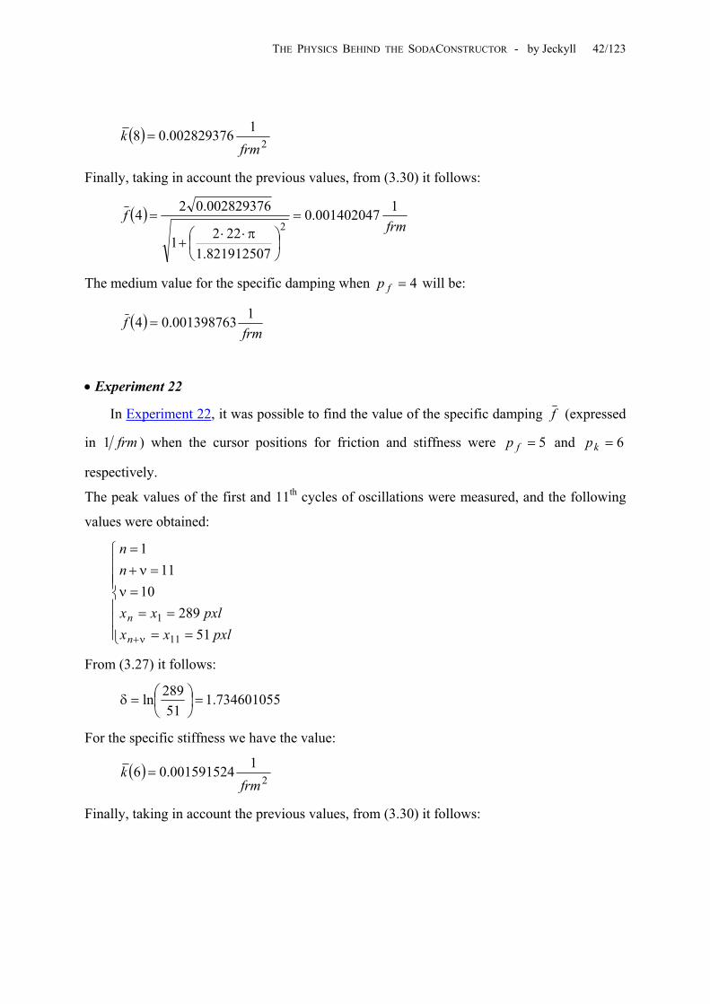
• Experiment 22
In Experiment 22, it was possible to find the value of the specific damping f (expressed
in frm1 ) when the cursor positions for friction and stiffness were and
respectively.
5=fp 6=kp
The peak values of the first and 11th cycles of oscillations were measured, and the following
values were obtained:
====
=ν=ν+
=
ν+ pxlxxpxlxx
nn
n
n
51289
1011
1
11
1
From (3.27) it follows:
734601055.151
289ln =
=δ
For the specific stiffness we have the value:
( )2
1001591524.06frm
k =
Finally, taking in account the previous values, from (3.30) it follows:

THE PHYSICS BEHIND THE SODACONSTRUCTOR - by Jeckyll 43/123
( )frm
f 1002201866.0
734601055.11021
001591524.0252=
π⋅⋅
+
=
• Experiment 23
In Experiment 23, it was possible to find the value of the specific damping f (expressed
in frm1 ) when the cursor positions for friction and stiffness were and
respectively.
5=fp 8=kp
The peak values of the first and 14th cycles of oscillations were measured, and the following
values were obtained:
====
=ν=ν+
=
ν+ pxlxxpxlxx
nn
n
n
55295
1314
1
14
1
From (3.27) it follows:
679642171.155295ln =
=δ
For the specific stiffness we have the value:
( )2
1002829376.08frm
k =
Finally, taking in account the previous values, from (3.30) it follows:
( )frm
f 1002187142.0
679642171.11321
002829376.0252=
π⋅⋅
+
=
The medium value for the specific damping when will be: 5=fp
( )frm
f 1002194504.05 =

THE PHYSICS BEHIND THE SODACONSTRUCTOR - by Jeckyll 44/123
• Results Analysis
As with the gravity and stiffness experiments, looking at the following Table 3.7, which
contains the values obtained in the previous virtual experiments, it is possible to establish that
the specific damping f is related to the cursor position by means of a quadratic
proportionality.
fp
Table 3.7: ratio between the specific damping and the cursor position
fp
frm
f 1
frmp
f
f
12
1 0.000087576 0.000087576
2 0.000350855 0.000087714
3 0.000791993 0.000087999
4 0.001398763 0.000087423
5 0.002194504 0.000087780
Just as with the previous physical quantities, it is possible to assume for the specific damping
the following law:
( )
⋅=
frmpfpf fpf
12 (3.31)
in which the value of the damping parameter pf can be obtained as medium value from the
values of the ratio 2fpf reported in the above Table 3.7. We will assume for the damping
parameter the following value:
frm
f p1000087698.0= (3.32)

THE PHYSICS BEHIND THE SODACONSTRUCTOR - by Jeckyll 45/123
In the following graph are reported both the experimental values of the specific damping and
the corresponding interpolation value obtained from (3.31) and (3.32).
fp
frm
f 1
1 2 3 4 5
0.0005
0.001
0.0015
0.002
Figure 3.10: Experimental and interpolating value for the specific damping.
3.5 COLLISIONS
The only collisions that exist in the sodaconstructor applet are collisions between masses
and walls12. There aren’t collisions between masses themselves: these entities, even though
they appear to have a particular size, are mathematically just points (i.e. couples of Cartesian
coordinates). For this reason we will avoid speaking in depth about this phenomenon. The
only thing that we need to understand is the way in which collisions between masses and rigid
walls occur.
There are two classic kinds of collisions: elastic and non-elastic. In elastic collisions, the
intensity of the velocity of a mass immediately before and after its impact on a rigid wall is
exactly the same. Only the direction of the velocity changes, depending on the angle of
impact. In non-elastic collisions, the velocity of the mass immediately after the impact drops
to zero. It is as if the wall were sprinkled with glue: the mass remains attached to the wall.
In reality, neither of these types of impacts exists. If elastic collisions existed in the real
world, then, in principle, it would be possible to have a ball that bounces on the ground
forever. Moreover, in reality, non-elastic collisions always result in at least a small recoil of
the mass.
12 By wall I mean the walls, the ground and the ceiling.

THE PHYSICS BEHIND THE SODACONSTRUCTOR - by Jeckyll 46/123
ou ov
tv tu
v u
Figure 3.11: velocities before and after an impact of a mass on a rigid wall.
We will define u and v, respectively, as the velocities of a mass immediately before and after
its collision with a rigid wall. In reference to the wall’s surface, we will indicate with and
their orthogonal components, and with u and their tangential components (see
Figure 3.11). It is possible to see in Figure 3.11 that the orthogonal components of velocities
have the opposite direction before and after the collision, while the tangential components of
velocities have the same direction before and after the collision. What about the values of
velocity?
ou
ov t tv
Since, as mentioned earlier, collisions in the real world will never be perfectly elastic or non-
elastic, in order to discuss mathematically exactly what happens during the impact of a mass
on a rigid wall, we will introduce the coefficients of elastic restitution and c . Thanks to
these coefficients, it is possible to write:
tc o
(3.33)
⋅=⋅=
ooo
ttt
ucvucv
Taking into account that in a realistic collision 0 , we can immediately understand
that the value of velocity after the impact is always less than the value of velocity before the
impact. Obviously, we would have a true elastic impact if the coefficients and were
equal to 1, and we would have a true non-elastic impact if the coefficients c and were
equal to 0.
1, << ot cc
tc
t
oc
oc

THE PHYSICS BEHIND THE SODACONSTRUCTOR - by Jeckyll 47/123
The question now is: what happens in the sodaconstructor applet? It easy to verify that in
collisions between masses and walls the masses always lose part of their kinetic energy13, so
in the next part of this section we will investigate the coefficients of elastic restitution of walls
in the sodaconstructor applet.
• The Coefficient of Elastic Restitution in the Orthogonal Impact
Thanks to the virtual experiment on orthogonal impact, it is possible to see that, in
absence of friction14, the maximum height of the free falling mass after each bounce is always
less than the previous. Calling u and v respectively the velocity of a mass immediately before
and after its impact on the ground, in accord with (3.33), the coefficient of elastic restitution
for the orthogonal impact will be:
uvco = (3.34)
In order to find the velocity of the mass immediately before the impact on the ground we will
use the well-known laws for uniformly accelerated motion. Using the height from which
the mass begins falling, on the ground the velocity will be:
1h
12ghu = (3.35)
What about the velocity v? We already know that the velocity v will be less than the velocity
u, so, inevitably, the height that the mass will reach after the first rebound must be less
than the high . It is possible to calculate the velocity v by simply measuring the height
reached by the mass after the first rebound:
2h
1h 2h
22ghv = (3.36)
13 i.e. the physical quantity related to the velocity of masses. 14 The damping in the previous section.

THE PHYSICS BEHIND THE SODACONSTRUCTOR - by Jeckyll 48/123
Taking into account (3.34), (3.35) and (3.36) we finally have:
1
2
1
2
2
2hh
gh
ghco == (3.37)
Measuring the heights and in the previous virtual experiment we find h and
. Applying the (3.37) we get:
1h 2h pxl4221 =
pxlh 2382 =
750986713.0422238
==oc
What does this mean? It means that in orthogonal impacts with the walls, free masses always
lose about 25% of their velocity!
• The Coefficient of Elastic Restitution in the Tangential Impact
In order to find the value of the coefficient of elastic restitution in tangential impacts, a
virtual experiment has been devised examining a particular tangential impact. In order to aid
the explanation of the experiment I have also realized the schematic Figure 3.12.
In this experiment, a mass with an initial horizontal velocity is free to fall in absence of
friction. The mass’s motion, in its parabolic falling, can be defined in two components: the
vertical motion and the horizontal motion. The vertical motion will be a uniformly accelerated
motion, while the horizontal motion will simply be a uniform motion15.
2d 1d
2h
1h
Figure 3.12: Scheme of the virtual experience
15 i.e. the horizontal component of velocity is constant.

THE PHYSICS BEHIND THE SODACONSTRUCTOR - by Jeckyll 49/123
Calling the height from which the mass starts its parabolic falling, the time it will take for
the mass to reach the ground is:
1h
gh
t 11
2= (3.38)
Calling the horizontal displacement of the mass in this time, the horizontal component of
the velocity will be:
1d
1
11
12hgd
td
u == (3.39)
This is the tangential velocity of the mass before the impact on the ground.
In order to calculate the coefficient of elastic restitution in the tangential impact now we need
the horizontal component of the velocity after the impact. It is possible to calculate this
velocity by considering that after the impact the motion of the mass can again be defined in
the two parts: the uniformly accelerated vertical motion and the uniform horizontal motion.
Therefore, calling the maximum height reached by the mass after the first rebound, the
time necessary to reach the ground again is:
2h
gh
t 22
22= (3.40)
Calling the horizontal displacement of the mass during this time, the horizontal
component of the velocity after the impact will be:
2d
2
2
2
222 h
gdtd
v == (3.41)

THE PHYSICS BEHIND THE SODACONSTRUCTOR - by Jeckyll 50/123
In accord with the first formula of (3.33), and taking into account the velocities (3.39) and
(3.41), the coefficient of elastic restitution for the tangential impact will be:
2
1
1
22 h
hd
duvct == (3.42)
From the virtual experiment mentioned earlier, it is possible to measure the following
distances:
====
pxlhpxlh
pxldpxld
23842257377
2
1
2
1
From (3.42) follows:
100663322.0238422
377257
=⋅
=tc
What does this mean? This means that in tangential impacts with the walls, free masses
always lose about 90% of their velocity! This fact is extremely enlightening (at least for me).
Indeed, it is the low value of this coefficient that allows our models to walk. In the applet,
there isn’t friction on the ground in the real physical meaning of the word. If the value of this
coefficient were greater, our models would walk with much difficulty. If this coefficient were
equal to 1, our models would not be able to walk at all.
3.6 FINAL RESULTS
At the end of this long chapter I will simply summarize in a concise way the main results
obtained by means of the previous virtual experiments.
We have defined with , and the position of the cursors of Figure 3.1. These
parameters can assume values from 0 to 107.
gp fp kp

THE PHYSICS BEHIND THE SODACONSTRUCTOR - by Jeckyll 51/123
The law of variation of the acceleration constant g with the cursor’s position is: gp
( )
⋅=
22
frmpxlpgpg gpg (3.43)
in which the value of the gravity parameter experimentally obtained is: pg
⋅= −
241050169.3
frmpxlg p (3.44)
The law of variation of the spring’s stiffness k with the cursor’s position is: kp
( ) ( )
( )
⋅=
⋅=
22 1
frmpkpk
mpkpk
kpk
kk
(3.45)
in which the value of the stiffness parameter pk experimentally obtained is:
⋅= −
25 1104209.4
frmk p (3.46)
The law of variation of the damping f with the cursor’s position is: fp
( ) ( )( )
⋅=
⋅=
frmpfpf
mpfpf
fpf
ff
12 (3.47)
in which the value of the damping parameter pf experimentally obtained is:

THE PHYSICS BEHIND THE SODACONSTRUCTOR - by Jeckyll 52/123
frm
f p1107698.8 5−⋅= (3.48)
The components of the velocity before and after an impact between masses and walls are
related by means of the equation:
(3.49)
⋅=⋅=
ooo
ttt
ucvucv
in which the values of the coefficients of elastic restitution experimentally obtained are:
(3.50)
≅≅
75.010.0
o
t
cc
All of the above constants are certainly affected by inevitable errors in the measurements, so I
would intuitively rely on just the first two significant digits. It would have been more
thorough to calculate the errors using the well-known statistical techniques, but since this is
all just play, I decided not to.
THE PHYSICS BEHIND THE SODACONSTRUCTOR - by Jeckyll 53/123
4. CINEMATIC
This chapter will discuss the main cinematic quantities16 that we will encounter in the
following chapter of this paper. These cinematic quantities are the position vector, the
velocity, and the acceleration. All are related to the masses on the screen17.
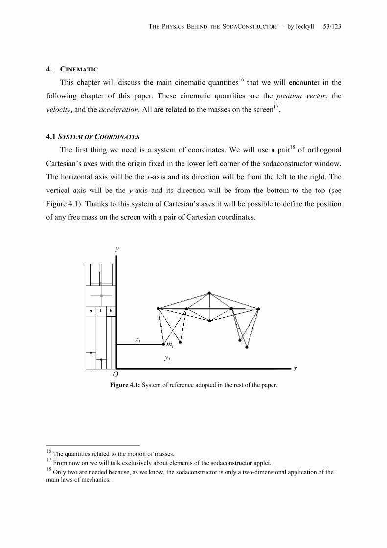
4.1 SYSTEM OF COORDINATES
The first thing we need is a system of coordinates. We will use a pair18 of orthogonal
Cartesian’s axes with the origin fixed in the lower left corner of the sodaconstructor window.
The horizontal axis will be the x-axis and its direction will be from the left to the right. The
vertical axis will be the y-axis and its direction will be from the bottom to the top (see
Figure 4.1). Thanks to this system of Cartesian’s axes it will be possible to define the position
of any free mass on the screen with a pair of Cartesian coordinates.
y
x
im ix
iy
O Figure 4.1: System of reference adopted in the rest of the paper.
16 The quantities related to the motion of masses. 17 From now on we will talk exclusively about elements of the sodaconstructor applet. 18 Only two are needed because, as we know, the sodaconstructor is only a two-dimensional application of the main laws of mechanics.

THE PHYSICS BEHIND THE SODACONSTRUCTOR - by Jeckyll 54/123
4.2 THE POSITION VECTOR
If N is the integer number of masses on the screen, each mass will be characterized by an
integer index included in the interval . So we will have: [ N,1 ]
)
Ni mmmmm ,,,,,, 321 LL
When we talk about a generic mass on the screen its index will be simply represented by the
letter i. So, very often, we will talk about the generic mass . im
Each mass on the screen will be located by a pair of Cartesian coordinates. In order to avoid
any confusion, each pair of coordinates will be characterized by the same index of the mass to
which they refer. So the generic mass will be located on the screen by the coordinates
(see Fig. 4.1).
im
( Niyx ii ,,2,1, K=
x
y
r
i
j
x
y
Figure 4.2: The position vector for the Cartesian point x, y.
In modern vector analysis a generic point in the space is located by a position vector. The
Cartesian point is given by the vector joining it to the origin of the coordinates (see
Fig 4.2). This vector can be written as:
( yx, )
(4.1) jir yx +=
THE PHYSICS BEHIND THE SODACONSTRUCTOR - by Jeckyll 55/123
where r is the position vector of the Cartesian point ( , and i and j are the unit vectors)
)
yx, 19 in
the x and y directions. Therefore the position vector for the generic mass will be
represented by:
im
(4.2) jir iii yx +=
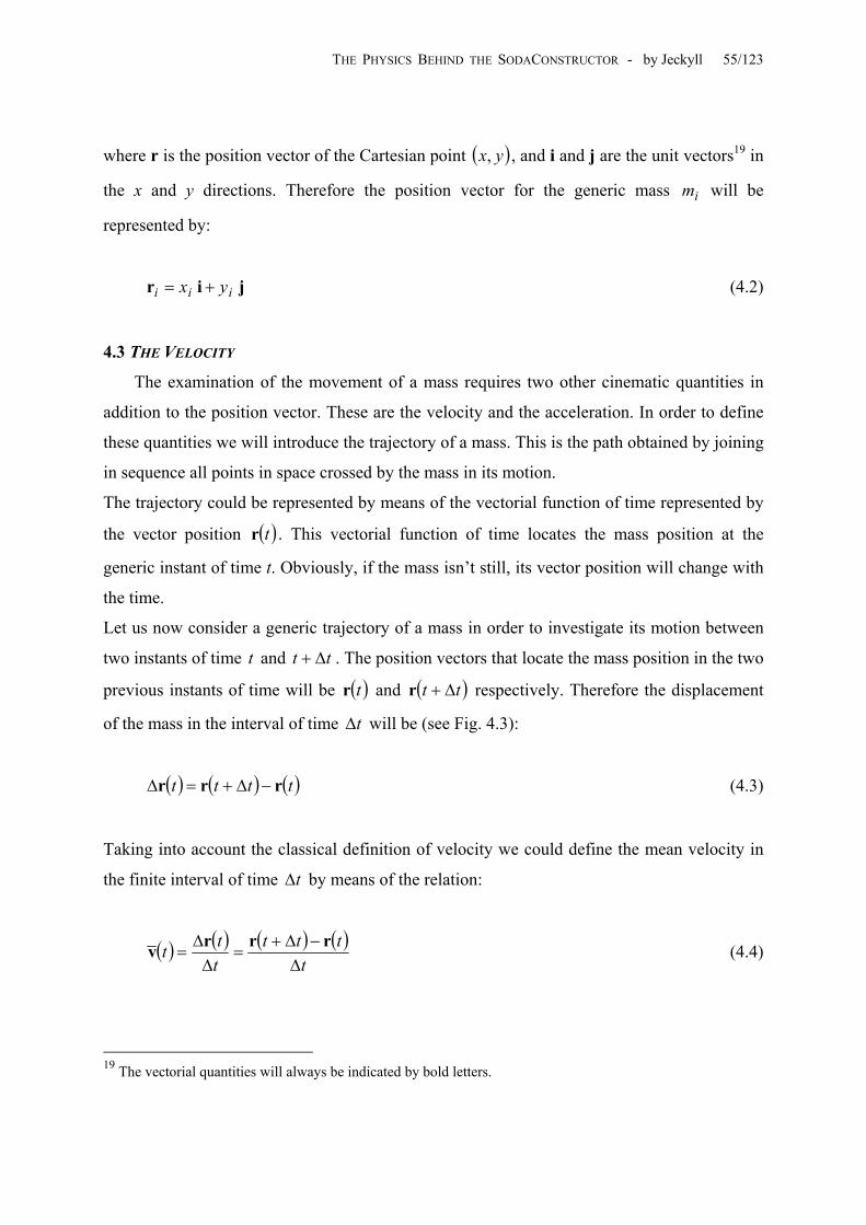
4.3 THE VELOCITY
The examination of the movement of a mass requires two other cinematic quantities in
addition to the position vector. These are the velocity and the acceleration. In order to define
these quantities we will introduce the trajectory of a mass. This is the path obtained by joining
in sequence all points in space crossed by the mass in its motion.
The trajectory could be represented by means of the vectorial function of time represented by
the vector position r . This vectorial function of time locates the mass position at the
generic instant of time t. Obviously, if the mass isn’t still, its vector position will change with
the time.
( )t
Let us now consider a generic trajectory of a mass in order to investigate its motion between
two instants of time and t . The position vectors that locate the mass position in the two
previous instants of time will be r and r respectively. Therefore the displacement
of the mass in the interval of time will be (see Fig. 4.3):
t t∆+
( )tt∆
( tt ∆+
(4.3) ( ) ( ) ( )tttt rrr −∆+=∆
Taking into account the classical definition of velocity we could define the mean velocity in
the finite interval of time by means of the relation: t∆
( ) ( ) ( ) ( )t
tttttt
∆−∆+
=∆∆
=rrrv (4.4)
19 The vectorial quantities will always be indicated by bold letters.

THE PHYSICS BEHIND THE SODACONSTRUCTOR - by Jeckyll 56/123
( )tr
( )tt ∆+r
( )tr∆
Figure 4.3: Displacement of a point in the interval of time ∆t.
If we would the instantaneous velocity of the mass at the time t we should consider the limit
of the mean velocity v as ∆ 0→t 20. Therefore the instantaneous velocity at time t will be
defined as:
( ) ( )ttt
vv0
lim→∆
= (4.5)
Remembering the definition of the position vector r we can write:
(4.6) ( ) ( ) ( )( ) ( ) (
∆++∆+=∆++=
jirjir
ttyttxtttytxt
)
so that the mean velocity (4.4) can be written as:
( ) ( ) ( ) ( ) ( ) jivt
tyttyt
txttxt∆
−∆++
∆−∆+
= (4.7)
Substituting (4.7) in (4.5) we get:
( ) ( ) ( ) ( ) ( ) ( )jivv
ttytty
ttxttxtt
ttt ∆−∆+
+∆
−∆+==
→∆→∆→∆ 000limlimlim (4.8)
20 We will read this to mean: “∆t approaches zero”.

THE PHYSICS BEHIND THE SODACONSTRUCTOR - by Jeckyll 57/123
Taking into account the definition of the derivative of a function we get the following
expression of velocity:
( ) ( ) ( )jiv
tdtyd
tdtxd
t += (4.9)
or, better:
(4.10) ( ) ( ) ( ) jiv tytxt && +=
This is exactly the expression of the velocity that we will use in the formulation of the
equations of motion for a model.
Obviously the velocity of the generic mass is: im
(4.11) ( ) ( ) ( ) jiv tytxt iii && +=
4.4 THE ACCELERATION
In addition to the velocity, it is possible to define the acceleration through the limit as
of the mean acceleration 0→∆t ( )ta :
( ) ( ) ( ) ( ) ( )t
ttttt
ttt ∆−∆+
=∆
∆==
→∆→∆→∆
vvvaa ttlimlimlim000
(4.12)
Taking into account the expression (4.10) for the velocity, from (4.12) follows:
( ) ( ) ( ) ( ) ( ) jiat
tyyt
txxttt ∆
−∆++
∆−∆+
=→∆→∆
&&&& ttlimttlim00
(4.13)
that is:

THE PHYSICS BEHIND THE SODACONSTRUCTOR - by Jeckyll 58/123
(4.14) ( ) ( ) ( ) jia tytxt &&&& +=
This is exactly the expression of the acceleration that we will use in the formulation of the
equations of motion for a model.
For the generic mass we also have: im
(4.15) ( ) ( ) ( ) jia tytxt iii &&&& +=
5. TOPOLOGY OF A MODEL
The first question about this chapter could be: What exactly is a model? Obviously we
need a definition. For this reason from now when we talk about a model we mean a system of
free masses21 themselves connected in various way by means of muscles and springs. And
what about the topology? The topology of a model is simply the exact way in which the
masses of a model are connected.
In order to define exactly the topology of a model let us consider a model made with N free
masses. We will indicate with the integer number the number of masses that are
connected with the generic free mass so that mass is connected with free masses,
mass connected with masses, and so on. Obviously for a model made with N free
masses we will have N integer numbers . These parameters are very important even if they
don’t say anything about the exact connections between the masses. The only thing that we
can determine with these parameters is that the mass is connected with other free
masses; nothing more. We still don’t know exactly which masses are connected to the mass
. For this reason we will introduce the topological index .
iN
1m
im
im
N
1N
N
2m 2N
i
i
im ijε
The topological index represents the index of the j-th mass connected with mass .
Obviously the index i and j will be such as:
ijε im
21 Fixed masses are not discussed in this article.

THE PHYSICS BEHIND THE SODACONSTRUCTOR - by Jeckyll 59/123
(5.1)
==
iNjNi
,,2,1,,3,2,1
K
K
In order to well understand the exact definition of the topological index let us consider the
following example. In the model of Figure 5.1 we have 8 free masses.
ijε
Figure 5.1: Example of a model
It is trivial to see that the mass is connected to 3 other masses, that mass is connected
to 3 other masses, that mass is connected to 4 other masses, and so on. By using the
definition of the parameter we can simply write:
1m
3m
2m
iN
.3;3;4;2;6;4;3;3
87
65
43
21
========
NNNNNNNN
But how are these masses connected? It is also trivial to see that the mass m is connected to
masses , m and , mass to masses , and m , and so on. Well, the values of
the topological index tell us exactly the way in which the masses are connected. In the present
case the values of the topological index are:
1
2m 4 6m 2m 1m 3m 4

THE PHYSICS BEHIND THE SODACONSTRUCTOR - by Jeckyll 60/123
.7;6;3;8;6;4
;8;7;4;1;4;3
;7;6;5;3;2;1;8;5;4;2
;4;3;1;6;4;2
838281
737271
64636261
5251
464544434241
34333231
232221
131211
=ε=ε=ε=ε=ε=ε
=ε=ε=ε=ε=ε=ε
=ε=ε=ε=ε=ε=ε=ε=ε=ε=ε
=ε=ε=ε=ε=ε=ε
The topological index will be very important when we need to sum the elastic forces acting on
a free mass in order to formulate the equations of motion for a model.

THE PHYSICS BEHIND THE SODACONSTRUCTOR - by Jeckyll 61/123
6. FORCES ANALYSIS
The movement of a mass is strictly related to the forces that are applied to the mass. For
this reason, in this chapter we will talk about the different kinds of forces that a mass might
encounter in its motion. There are essentially three such forces: the gravity forces, the
damping forces (the friction), and the elastic forces.
6.1 THE GRAVITY FORCES
Regarding the gravity forces, to tell the truth, there isn’t much to say. Each free mass will
be subjected to a weight force that is proportional to the mass value by means of the constant
g. In the applet, all free masses are the same, so each mass will be subjected to the force:
(6.1) Nigmgmigi ,,2,1 K=−=−= jjF
where the symbol m has been assumed for the common value of all the masses. Obviously, in
order to express the weight force, we need the unit vector j of the y-axis. Finally the minus
sign in (6.1) means that gravity pushes the masses down. When the gravity reverse option in
the applet is activated the expression (6.1) simply becomes:
(6.2) Nigmgmigi ,,2,1 K=== jjF
6.2 THE DAMPING FORCES
We already talked about the damping forces when we studied the free damped vibrations
of a spring-mass system in order to calculate experimentally the damping constant of the
applet. We have already said that a mass in motion in a viscous fluid with velocity v is
subjected to a force F equal to (see Fig. 3.8):
(6.3) vF f−=
Now, thanks to what we have already said in sections 3.4 and 4.3, we can write a more
appropriate expression for the damping force acting on a generic mass m : i

THE PHYSICS BEHIND THE SODACONSTRUCTOR - by Jeckyll 62/123
(6.4) ( ) ( ) Nitft if
i ,,2,1 K=−= vF
from which, thanks to the expression of velocity (4.11), follows:
(6.5) ( ) ( ) ( )[ ] Nitytxft iif
i ,,2,1 K&& =+−= jiF
Finally, taking into account the first expression of (3.47), we will write:
( ) ( ) ( )[ ] Nitytxfmt iif
i ,,2,1 K&& =+⋅⋅−= jiF (6.6)
in which has been introduced the specific damping constant f .
6.3 THE ELASTIC FORCES
The discussion of the elastic forces acting on a specific mass of a model is a little bit
more complex, essentially for two reasons. The first is that each mass of a model is generally
connected to more masses, so that often many elastic forces act upon a single mass. The
second is that the elastic forces acting on a mass can come from springs or muscles. So, in
order to find the exact expression for the resultant of many elastic forces acting on a single
generic mass, we must first study springs and muscles. We will do this in the next chapter, so
here we will talk about the elastic forces in general.
We have already talked about the elastic forces of a spring in section 3.2. In that section we
said that a spring of original length extended until the length l ( l ) needs a traction
force of intensity F proportional to the extension ∆ by means of the stiffness constant
k (see Fig. 3.5):
0l 0l>
0lll −=
(6.7) lkF ∆⋅=

THE PHYSICS BEHIND THE SODACONSTRUCTOR - by Jeckyll 63/123
This is valid, obviously, from the spring’s point of view. But now we are investigating the
forces acting on the free masses by means of springs. These forces, thanks to Newton’s third
law22, are equal in intensity to the forces acting on the springs but with opposite direction.
Therefore, when a spring is extended, the forces act on the free masses at its extremities
pushing them toward each other. Instead, when a spring is compressed, the forces act on the
free masses at its extremities pushing them away from each other (see Fig. 6.1).
0l
01 ll >
02 ll <
1F 1F 1F 1F
2F 2F 2F 2F
Figure 6.1: Forces acting on the masses at the end of a spring.
7. SPRINGS AND MUSCLES
In order to get the exact expression for the resultant of elastic forces acting on a generic
mass , we must first investigate springs and muscles. Without any delay, let us begin these
investigations.
im
7.1 THE SPRINGS
Let us consider a spring that connects two free masses, and , in a hypothetical
model. We will indicate with l the length at rest of the spring that connects masses i and j.
This length is the length assigned to the spring when the two masses are originally connected
im jm
rij
22 The principle of action and reaction.

THE PHYSICS BEHIND THE SODACONSTRUCTOR - by Jeckyll 64/123
in the applet’s construct mode. This value will never change during the simulation, and is
important in order to evaluate the elastic forces acting on the masses m and . i jm
tlij
We will indicate with the effective length of a spring during the simulation. Obviously
this length will change continuously so it will be a function of time. Its value is determined by
the coordinates of its extremities; i.e. its value depends on the coordinates of the free masses
and . Therefore, applying the well-known Theorem of Pythagoras we have (see
Fig. 7.1):
( )tlij
im jm
( ) ( ) ( )[ ] ( ) ( )[{ ] }21
22 tytytxtxtl jijiij −+−= (7.1)
jm
im
jx
jy
( )tlij
ix
iy
x
y
Figure 7.1: Length of a spring.
The stretch of the spring ij in the generic instant of time t is:
(7.2) ( ) ( ) rijijij ltltl −=∆
Therefore, when , the spring is in traction, while when , the spring is in
compression. As we discussed in the previous chapter, when the spring ij is in traction, the
elastic forces acting on masses i and j will push them together, and when the spring ij is in
compression, the elastic forces acting on masses i and j will push them apart. The direction of
these forces, whatever the sign of may be, will correspond with the direction of the
( ) 0>∆ tlij ( ) 0<∆
( )tlij∆
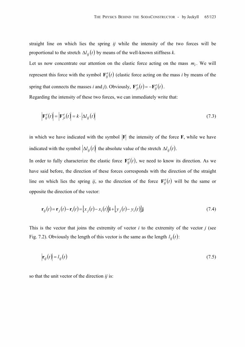
THE PHYSICS BEHIND THE SODACONSTRUCTOR - by Jeckyll 65/123
straight line on which lies the spring ij while the intensity of the two forces will be
proportional to the stretch by means of the well-known stiffness k. ( )tlij∆
( )tlij∆
Let us now concentrate our attention on the elastic force acting on the mass . We will
represent this force with the symbol (elastic force acting on the mass i by means of the
spring that connects the masses i and j). Obviously, .
im
( )teijF
( ) ( )tt eij
eji FF −=
Regarding the intensity of these two forces, we can immediately write that:
( ) ( ) (7.3) ktt eji
eij ⋅== FF
in which we have indicated with the symbol F the intensity of the force F, while we have
indicated with the symbol ( )tlij∆ the absolute value of the stretch . ( )tlij∆
In order to fully characterize the elastic force , we need to know its direction. As we
have said before, the direction of these forces corresponds with the direction of the straight
line on which lies the spring ij, so the direction of the force F will be the same or
opposite the direction of the vector:
( )teijF
( )teij
( ) ( ) ( ) ( ) ( )[ ] ( ) ( )[ ]jirrr tytytxtxttt ijijijij −+−=−= (7.4)
This is the vector that joins the extremity of vector i to the extremity of the vector j (see
Fig. 7.2). Obviously the length of this vector is the same as the length : ( )tlij
( ) ( )tlt ijij =r (7.5)
so that the unit vector of the direction ij is:

THE PHYSICS BEHIND THE SODACONSTRUCTOR - by Jeckyll 66/123
( )( )( )
( ) ( )( )
( ) ( )[ ] ( ) ( )[ ]( ) ( )[ ] ( ) ( )[ ]22
ˆtytytxtx
tytytxtxtl
tttlt
tijij
ijij
ij
ij
ij
ijij
−+−
−+−=
−==
jirrrr (7.6)
( )tir( )tjr
( )tijr
x
y
Figure 7.2: The vector r ( )tij
The unit vector r , like the vector , is directed from i to j. This is the same as the
direction of the elastic force F when the stretch is positive. Therefore we can
write a general expression of the force simply by multiplying with :
( )tijˆ ( )tijr
( )teijF
( )teij ( )tlij∆
( )tlk ij∆⋅ ( )tijr̂
(7.7) ( ) ( ) ( )ttlkt ijijeij rF ˆ∆⋅=
This expression is valid in general. Indeed, if the stretch is positive, then as we have stated
before, the force acting on the mass i will directed from i to j like the unit vector r , while,
if the stretch is negative, the force acting on the mass i will be directed from j to i, like the
direction of the vector obtained by multiplying a negative quantity ( ) with the unit
vector r .
( )tijˆ
( )tlij∆
( )tijˆ
Using the previous expressions (7.1), (7.2) and (7.6), from (7.7) we get a more explicit
expression for the elastic force F : ( )teij
( ) ( )[ ] ( )( )tlt
ltlktij
ijrijij
eij
rF −= (7.8)

THE PHYSICS BEHIND THE SODACONSTRUCTOR - by Jeckyll 67/123
where:
( ) ( ) ( )[ ] ( ) ( )[ ]
( ) ( ) ( )[ ] ( ) ( )[ ]
−+−=
−+−=
jir tytytxtxt
tytytxtxtl
ijijij
ijijij22
(7.9)
7.2 THE MUSCLES
We all know what a spring is. We have all seen real springs in our own lives. But what
exactly is a muscle? In the sodaconstructor, muscles are simply springs with the length at rest
changing in time with harmonic law. Certainly, this sort of object doesn’t exist in the real
world. In reality a spring’s length at rest doesn’t change over time. Muscles are simply
abstract objects invented by Ed Burton (I suppose) in order to give energy to our models. You
could say that the sodaconstructor muscle is a simplified version of the human muscle.
rijl
In order to define mathematically these new entities, let us consider two free masses and
connected by a muscle. As stated before, the length at rest of the muscle is:
im
jm
(7.10) ( ) ([ ijijijrij tltl ϕ+ω⋅β⋅α+= sin10 )]
where a lot of new parameters have been introduced. The parameters in (7.10) that have the
index ij are parameters closely related to the specific muscle that joins the masses i and j.
These parameters ( ) can be different for each muscle of a model. The other
parameters (β ) are valid for all the muscles of a model.
ijijijl ϕα ,,0
ω,
The first and most intuitive parameter that has been introduced in (7.10) is the length . This
length is the length assigned to the muscle when the two masses are originally connected in
the applet’s construct mode. If this were a spring and not a muscle, the length l would
simply be the length at rest .
0ijl
0ij
rijl

THE PHYSICS BEHIND THE SODACONSTRUCTOR - by Jeckyll 68/123
In order to explain all the other new parameters in (7.10) we will refer to the
sodaconstructor’s muscle control panel, as shown in the following Figure 7.3:
ωijϕ
ijα
β
rad4π
rad2π
rad4
3π
Figure 7.3: muscle control panel.
Let us go in order:
• is the parameter that determines the speed of the oscillation for all the muscles in a
model. Its value is expressed in
ω
frmrad and it can be changed with the cursor shown in
Figure 7.3. When this cursor is placed on the top, as everyone knows, the value of the
parameter is zero. We could define in the following various ways: pulsation,
frequency, circular frequency, etc.
ω ω
• is the parameter of phase for the specific muscle ij. By adjusting this parameter we set
the delay before muscle ij reaches its maximum amplitude. In Figure 7.3 it is possible to
see the value of the phase ϕ in the muscles control panel. When the phase cursor is on
the top the phase is equal to . The intermediate positions correspond
respectively the values of
ijϕ
ij
radij 0=ϕ
rad4π , rad2π and rad4π3 . Thanks to this parameter, the
model constructors are able to synchronize harmoniously the movement of their precious
and spectacular models ;)

THE PHYSICS BEHIND THE SODACONSTRUCTOR - by Jeckyll 69/123
• is the parameter that fixes the wave amplitude. This parameter can assume any value in
the interval [ . When the sinusoidal wave is simply a straight line, the value of the
parameter is 0. When the wave has the maximum amplitude β is equal to 1 (see
Fig. 7.3). Obviously, the value of is the same for all the muscles of a model.
β
]1,0
β
β
• is the parameter that determines the benefit of the wave amplitude β for the muscle ij
(its relative amplitude). Just like the amplitude β , can assume all the values in the
interval [ . α is equal to 0 when the position of the cursor (see Fig. 7.3) is completely
on the left, while is equal to 1 when the cursor is completely on the right.
ijα
ijα
]1,0 ij
α ij
In order to better understand these parameters let us consider a few examples. The first
example that I want to take into consideration is the case of a free muscle with α . In
this case, (7.10) becomes:
1=β=ij
(7.11) ( ) ([ ijijrij tltl ϕ+ω+= sin10 )]
which shows that the length of the free muscle will change periodically from 0 to . 02 ijl
The second example that I want to take into consideration is the case of a muscle with
. In this case, no matter what the value of the amplitude, from (7.11) simply follows: 0=α ij
(7.12) ( ) 0ij
rij ltl =
In this case the muscle becomes a spring. For this reason, it is absolutely valid to think of all
springs as muscles with the parameter α . 0=ij
What about the forces acting on the masses at the extremities of a muscle? The expression of
these forces is exactly the same as it is with the elastic forces due to springs. The only
difference is in the expression of the length l : for springs this length is constant, while for
muscles this length changes over time with the law (7.10).
rij
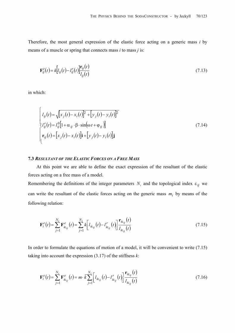
THE PHYSICS BEHIND THE SODACONSTRUCTOR - by Jeckyll 70/123
Therefore, the most general expression of the elastic force acting on a generic mass i by
means of a muscle or spring that connects mass i to mass j is:
( ) ( ) ( )[ ] ( )( )tlt
tltlktij
ijrijij
eij
rF −= (7.13)
in which:
( ) ( ) ( )[ ] ( ) ( )[ ]( ) ( )[( ) ( ) ( )[ ] ( ) ( )[ ]
−+−=
ϕ+ω⋅β⋅α+=
−+−=
jir tytytxtxt
tltl
tytytxtxtl
ijijij
ijijijrij
ijijij
sin10
22
] (7.14)
7.3 RESULTANT OF THE ELASTIC FORCES ON A FREE MASS
At this point we are able to define the exact expression of the resultant of the elastic
forces acting on a free mass of a model.
Remembering the definitions of the integer parameters and the topological index we
can write the resultant of the elastic forces acting on the generic mass by means of the
following relation:
iN ijε
im
( ) ( ) ( ) ( )( )( )∑∑
= ε
ε
εε=
ε
−==
i
ij
ij
ijij
i
ij
N
j i
irii
N
j
ei
ei tl
ttltlktt
11
rFF (7.15)
In order to formulate the equations of motion of a model, it will be convenient to write (7.15)
taking into account the expression (3.17) of the stiffness k:
( ) ( ) ( ) ( )( )( )∑∑
= ε
ε
εε=
ε
−⋅==
i
ij
ij
ijij
i
ij
N
j i
irii
N
j
ei
ei tl
ttltlkmtt
11
rFF (7.16)

THE PHYSICS BEHIND THE SODACONSTRUCTOR - by Jeckyll 71/123
There is one last question about the mathematical expression of elastic forces. What happens
when two masses are in same place on the screen? This event, even if it isn’t realistic,
physically speaking, could happen23. In this case the expression (7.8) becomes indeterminate
(mathematically we have met an indetermination of the kind 00 ). The soda algorithm must
have some control in order to avoid an error like the division by zero error. I’ve verified that
this control effectively exists through a demonstration in the following Example in which two
masses are perfectly overlapped. The applet simply fails to take into consideration the elastic
forces between masses that are perfectly overlapped.
23 In linear motors, for example, this happens systematically.

THE PHYSICS BEHIND THE SODACONSTRUCTOR - by Jeckyll 72/123
8 EQUATIONS OF THE MOTION OF A MODEL
We now have all the expressions of the forces that could act on a generic mass . These
forces are:
im
• The gravity force:
(8.1) jF gmgi −=
• The damping force:
( ) ( ) ( )[ jiF tytxfmt iif
i && +⋅⋅−= ] (8.2)
• The elastic force:
( ) ( ) ( )( ) ( )[ ] ( ) ( )[ ]
( )∑= ε
εε
εε
−+−
−⋅=
i
ij
ijij
ijij
N
j i
iirii
ei tl
tytytxtxtltlkmt
1
jiF (8.3)
Therefore their resultant will be: ( )tiF
(8.4) ( ) ( ) ( )ttt ki
fi
gii FFFF ++=
Combining the two directional components x and y, the resultant can be written as: ( )tiF
(8.5) ( ) ( ) ( ) jiF tFtFt yi
xii +=
where the expressions of the components and , according to (8.1,2,3,4), can be
written as:
( )tF xi ( )tF y
i

THE PHYSICS BEHIND THE SODACONSTRUCTOR - by Jeckyll 73/123
( ) ( ) ( ) ( )( ) ( )[ ]
( )
( ) ( ) ( ) ( )( ) ( )[
( )]
−
−+−−=
−
−+−=
∑
∑
= ε
εεε
= ε
εεε
i
ij
ij
ijij
i
ij
ij
ijij
N
j i
iriii
yi
N
j i
iriii
xi
tl
tytytltlktyfgmtF
tl
txtxtltlktxfmtF
1
1
&
&
(8.6)
In order to get the system of differential equations that governs the motion of a model, we will
apply Newton’s second law to all the N masses of the model. Therefore, we will have:
(8.7) ( ) ( ) Nitmt ii ,,2,1 K== aF
or, taking into account the expressions (4.15) and (8.5), also:
(8.8) ( ) ( ) ( ) ( )[ ] NitytxmtFtF iiy
ix
i ,,2,1 K&&&& =+=+ jiji
Assembling together the components of x and y of all these equations and taking into account
expressions (8.6) of the components and we will get: ( )tF xi ( )tF y
i
( ) ( ) ( ) ( )( ) ( )[ ]
( )
( ) ( ) ( ) ( )( ) ( )[ ]
( )
Ni
tl
tytytltlktyfgmtym
tl
txtxtltlktxfmtxm
i
ij
ij
ijij
i
ij
ij
ijij
N
j i
iriiii
N
j i
iriiii
,,2,1
1
1K
&&&
&&&
=
−
−+−−=
−
−+−=
∑
∑
= ε
εεε
= ε
εεε
(8.9)
At this point it is possible to definitively solve the mystery of the value of the mass m. As
stated in Chapter 2, it isn’t necessary to assume any specific value for the mass m, consistent
to all the free masses in the applet. Indeed, whatever the value of m might be, in (8.9) it can be
seen that the constant m can be simplified everywhere. Obviously this is possible only
because all masses in the applet are the same24.
24 i.e. all the masses have the same inertial properties.

THE PHYSICS BEHIND THE SODACONSTRUCTOR - by Jeckyll 74/123
The equations (8.9) can more conveniently be written as:
( ) ( ) ( )( ) ( ) ( )
Nityyyxxxftyftytyyyxxxftxftx
NNy
iii
NNx
iii ,,2,1,,,,,,,,,,,,,,,,
2121
2121 KKK&&&
KK&&&=
=+=+ (8.10)
in which the known scalar functions and have the expressions: xif y
if
( ) ( ) ( )( ) ( )[ ]
( )
( ) ( ) ( )( ) ( )[ ]
( )
−
−+−=
−
−=
∑
∑
= ε
εεε
= ε
εεε
i
ij
ij
ijij
i
ij
ij
ijij
N
j i
iriiNN
yi
N
j i
iriiNN
xi
tl
tytytltlkgtyyyxxxf
tl
txtxtltlktyyyxxxf
12121
12121
,,,,,,,,
,,,,,,,,
KK
KK
(8.11)
The equations (8.10) represent a system of non-linearN2 25 differential equations of second
order in unknown functions represented by the coordinates of the model’s free masses
. Thanks to the numerical resolution
N2
( ) [it( ) ],,2,1, Nytx ii K= 26 of this system of equations
we can determine the movement of our model over time.
9. NUMERICAL RESOLUTION OF THE EQUATIONS OF MOTION
In the past, even though many problems were already formulated in terms of differential
equations, their exact resolutions27 weren’t always obtainable. Only in a few cases was it
possible to obtain an exact solution; in all the remaining cases almost nothing could be done.
Sometimes it was possible to use approximate methods of resolution, but in these methods a
lot of calculus had to be done. Today, thanks to our beloved computers, this isn’t a problem
anymore. Today we have at our disposal a large amount of numerical techniques that allow us
to get a resolution of any differential problem with the accuracy wanted. Finding a solution to
a problem like those defined in equations (8.10) and (8.11) only thirtyfive years ago would
25 The functions and are non-linear functions. x
ify
if26 Unfortunately, the resolution (integration) of the equations (8.11) is possible only in a numerical way. 27 i.e. the resolution in terms of well-known mathematical functions.

THE PHYSICS BEHIND THE SODACONSTRUCTOR - by Jeckyll 75/123
have required the computers of NASA. Today, there are a variety of pocket videogames that
are able to solve problems more complex than ours. Today it might also be accurate that the
true power of a nation is in the capacity of her computers to go fast (capacity expressed in
billions of calculus per second).
Here I will show you the simplest numerical technique that we need in order to solve the
equations of motion (8.10). This numerical technique, usually called the finite differences, as
well as all the other more sophisticated numerical techniques, will transform the system of
differential equations (8.10) into a system of algebraic equations that, step by step, allow us to
get the positions of the masses of a model over time.
In order to pursue this objective we absolutely need some approximated expressions for the
scalar velocities , and the scalar accelerations , . Therefore we will start
looking for an approximated expression for the first derivative of a generic real function
. We know that the exact expression of the first derivative of a function is defined
by the limit:
( )txi& ( )tyi& ( )txi&& ( )tyi&&
( )xf ( )xf
( ) ( ) ( )x
xfxxfxfx ∆
−∆+=′
→∆ 0lim (9.1)
Looking at this definition it is immediately possible to understand that an approximate value
for the first derivative could be calculated choosing a very small value of the finite
interval . Therefore the expression:
( )xf ′
x∆
( ) ( ) ( )x
xfxxfxf∆
−∆+≅′ (9.2)
will be more accurate as gets smaller, so that we will use this expression in order to
approximate the first derivative of a function.
x∆
What about the second derivative ? By definition we can write: ( )xf ′′
( ) ( ) ( )x
xfxxfxfx ∆
′−∆+′=′′
→∆ 0lim (9.3)

THE PHYSICS BEHIND THE SODACONSTRUCTOR - by Jeckyll 76/123
so that, just like the first derivative, the approximate expression for the second derivative will
be:
( ) ( ) ( )x
xfxxfxf∆
′−∆+′≅′′ (9.4)
This expression isn’t particularly useful because it contains the first derivative of the function
. Therefore, since from expression (9.2) follows: ( )xf
( ) ( ) ( )x
xxfxxfxxf∆
∆+−∆+≅∆+′ 2 (9.5)
substituting (9.2) and (9.5) in the approximate expression of the second derivative (9.4) we
get:
( ) ( ) ( ) ( )2
22x
xfxxfxxfxf∆
+∆+−∆+≅′′ (9.6)
In order to evaluate the approximate expressions of the first and second derivatives of the
unknown function of our problem we will use respectively the relations (9.2) and (9.6). We
will have:
( ) ( ) ( )
( ) ( ) ( )
( ) ( ) ( ) ( )
( ) ( ) ( ) ( )
∆
+∆+−∆+≅
∆
+∆+−∆+≅
∆−∆+
≅
∆−∆+
≅
2
2
22
22
t
tyttyttyty
t
txttxttxtx
ttytty
tyt
txttxtx
iiii
iiii
iii
iii
&&
&&
&
&
(9.7)
These expressions will be more accurate as the finite interval of time ∆ is smaller. t

THE PHYSICS BEHIND THE SODACONSTRUCTOR - by Jeckyll 77/123
Using the approximate expression (9.7) in the equations of motion (8.10) we get:
( ) ( ) ( ) ( ) ( ) ( )( ) ( ) ( ) ( ) ( ) ( )
Nitf
ttytty
ft
tyttytty
tft
txttxf
ttxttxttx
yi
iiiii
xi
iiiii
,,2,122
22
2
2K=
=∆
−∆++
∆
+∆+−∆+
=∆
−∆++
∆
+∆+−∆+
(9.8)
from which follows:
( ) ( ) ( ) ( ) ( ) ( )( ) ( ) ( ) ( ) ( ) ( )
Nittftytfttytfttyttftxtfttxtfttx
yiiii
xiiii ,,2,1
122122
2
2K=
∆+−∆+∆+∆−=∆+∆+−∆+∆+∆−=∆+ (9.9)
These expressions are very important in finding the approximate solutions of the equations
(8.10) because they allow us to find the position of all N masses of a model in the instant of
time , while previously we knew the position of all N masses in the instants of time
and t. This means that if we know the positions and velocities of all the masses in a
particular instant of time, using the relations (9.9) iteratively we will be able to get the
evolution of the position of all the masses over time; i.e. the movement of our model. The
positions and the velocities of all the masses in a particular starting instant are called initial
conditions, and they are fundamental in order to solve numerically our differential equations.
tt ∆+ 2
tt ∆+
Above I said that using the equations (9.9) iteratively it is possible to calculate the positions
of the masses of a model over time. But what exactly does it mean to use the equations
iteratively? In order to understand this let us introduce the following position:
(9.10)
( )( )( )( )
∞=
=
=
=
=
∆+= −
,,3,2,1
1
Kj
ftfftf
ytyxtx
ttt
yijj
yi
xijj
xi
jiji
jiji
jj
If we choose as the initial instant the generic time t , from the first of (9.10) follows: k

THE PHYSICS BEHIND THE SODACONSTRUCTOR - by Jeckyll 78/123
(9.11)
∆+=∆+=∆+=
++
+
tttttttt
kkk
kk
212
1
from which it is possible to see that the three instants of time t , and are in a series
like the three instants of time t, and t from (9.9). Therefore, these relations can
also be written as:
k 1+kt 2+kt
tt ∆+ t∆+ 2
( ) ( ) ( ) ( ) ( ) ( )( ) ( ) ( ) ( ) ( ) ( )
Nittftytftytftyttftxtftxtftx
ky
ikikiki
kx
ikikiki ,,2,11212
212
212 K=
∆+−∆+∆−=∆+−∆+∆−=
++
++ (9.12)
or better:
( ) ( )( ) ( ) Ni
tfytfytfytfxtfxtfx
yik
ki
ki
ki
xik
ki
ki
ki ,,2,1
1212
212
212K=
∆+−∆+∆−=∆+−∆+∆−=
++
++ (9.13)
from which it is possible to understand how, by simply knowing the positions of all the
masses of a model in the two instants of time and t , it is possible to get the positions of
the same masses in the next instant of time . Since the instant of time is totally
arbitrary, it is also possible to understand how the relations (9.13) are absolutely general.
Therefore these relations can be used iteratively in order to find how the positions of the
masses of a model change over time. Indeed, if we know, for example, the positions of the
free masses of a model in the instants of time and , thanks to (9.13) it is possible to find
the position of the masses in the instant of time . Then, applying (9.13) once again, it will
be possible to find the position of all the masses at the instant of time t . In this way, we can
find the positions of all the masses at the instants of time t , t , t and so on indefinitely.
kt
t
0t
1+k
1t
2+k
2t
kt
3
4 5 6
Before I close this chapter I will say one more thing. The expressions (9.13) might appear to
be very simple and fast in application, but it is important to remember that the terms and xikf
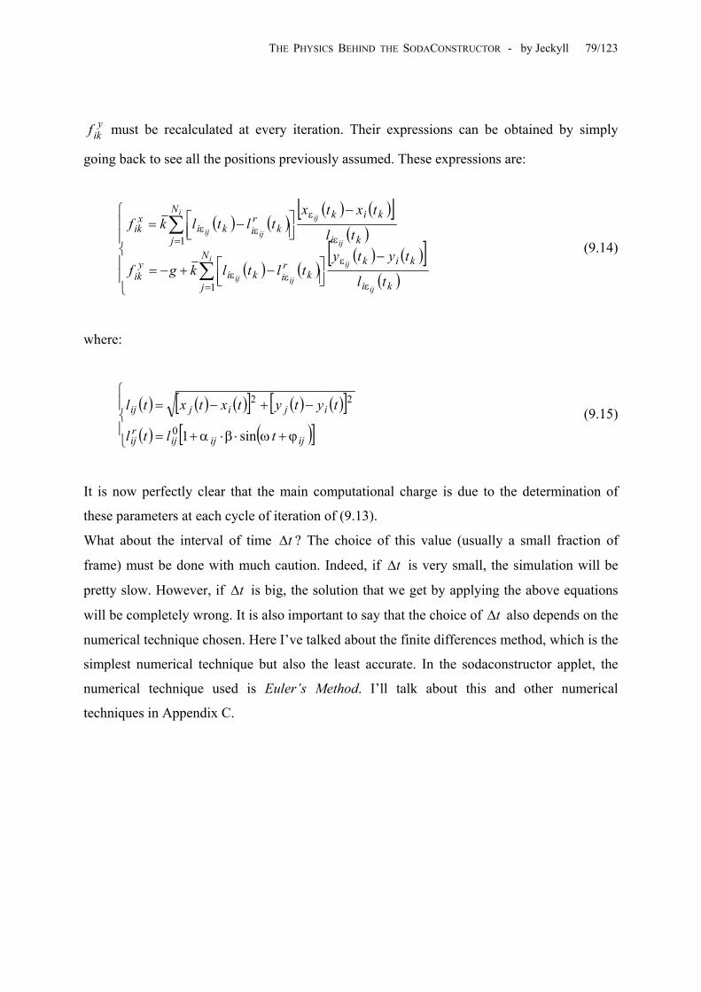
THE PHYSICS BEHIND THE SODACONSTRUCTOR - by Jeckyll 79/123
yikf must be recalculated at every iteration. Their expressions can be obtained by simply
going back to see all the positions previously assumed. These expressions are:
( ) ( )( ) ( )[ ]
( )
( ) ( )( ) ( )[
( )]
−
−+−=
−
−=
∑
∑
= ε
ε
εε
= ε
ε
εε
i
ij
ij
ijij
i
ij
ij
ijij
N
j ki
kikk
riki
yik
N
j ki
kikk
riki
xik
tl
tytytltlkgf
tl
txtxtltlkf
1
1 (9.14)
where:
( ) ( ) ( )[ ] ( ) ( )[ ]( ) ( )[ ]
ϕ+ω⋅β⋅α+=
−+−=
ijijijrij
ijijij
tltl
tytytxtxtl
sin10
22 (9.15)
It is now perfectly clear that the main computational charge is due to the determination of
these parameters at each cycle of iteration of (9.13).
What about the interval of time ? The choice of this value (usually a small fraction of
frame) must be done with much caution. Indeed, if ∆ is very small, the simulation will be
pretty slow. However, if ∆ is big, the solution that we get by applying the above equations
will be completely wrong. It is also important to say that the choice of also depends on the
numerical technique chosen. Here I’ve talked about the finite differences method, which is the
simplest numerical technique but also the least accurate. In the sodaconstructor applet, the
numerical technique used is Euler’s Method. I’ll talk about this and other numerical
techniques in Appendix C.
t∆
t
t
t∆

THE PHYSICS BEHIND THE SODACONSTRUCTOR - by Jeckyll 80/123
10. THE STATIC AND QUASI-STATIC SIMPLIFIED PROBLEM
The previous equations of motions (8.9) were obtained simply by applying Newton’s
second law to each mass of a model. The terms strictly related to the motion of free masses
arise in these equations. These terms are the damping forces and the inertial forces28. These
terms are respectively related to the velocities and the accelerations of the free masses. In
many cases, however, the movement of the model could be so slow that these forces become
themselves negligible. In these cases the only forces acting on a model are the elastic forces29.
To study the movement of the model in these situations, it is only necessary to consider the
elastic forces, like in the static case. Therefore, when we study a model without taking into
account inertial forces or damping forces, we will say that we are studying a quasi-static
model.
In this chapter, we will be able to solve many practical problems simply by not taking these
forces into account.
10.1 SYSTEM OF EQUATIONS
By ignoring the damping and inertial forces, from the equations (8.9) follows this system
of equations:
Ni
l
yyll
l
xxll
i
ij
ij
ijij
i
ij
ij
ijij
N
j i
irii
N
j i
irii
,,2,10
0
1
1K=
=−
−
=−
−
∑
∑
= ε
εεε
= ε
εεε
(10.1)
in which the time hasn’t even been taken into account. This is because even if we have
muscles in the model, the solution of the problem would be determined instant after instant.
Therefore, in principle, there is no difference between the static case and the quasi-static case.
In any case, we will only consider springs.
The system of equations (10.1) can be more conveniently written as:
28 in the sense of d’Alembert’s principle. 29 and, eventually, the gravity forces.

THE PHYSICS BEHIND THE SODACONSTRUCTOR - by Jeckyll 81/123
( )
( )Ni
yyl
l
xxl
l
i
ijij
ij
i
ijij
ij
N
ji
i
ri
N
ji
i
ri
,,2,1
01
01
1
1K=
=−
−
=−
−
∑
∑
=ε
ε
ε
=ε
ε
ε
(10.2)
where:
( ) ( )22iii yyxxl
ijijij−+−= εεε (10.3)
In this system of equations the data are the lengths at rest of all the springs in the model, while
the unknown quantities are the coordinates of the free masses in the equilibrium
configuration.
Before we examine some applications of quasi-static problems, it is important to explain a
few things about the system of equations (10.2). First, this system of equations isn’t linear.
This fact could be a big problem, because there is no general way to solve non-linear systems
of equations. Some solutions can be obtained in particular cases, but in all the remaining cases
the only way to solve the system of equations is to use numerical algorithms. The simplest
numerical algorithm for the resolution of non-linear systems of equations is the generalization
for more than one non-linear equation of Newton’s algorithm30. Initially, I planned to add a
short paragraph about this method, but for now I have changed my mind. The main reason is
that we will not really need to solve the (10.2) system of equations in order to study practical
problems in the ordinary life of a typical sodaconstructorman/woman. As we will see, it is
possible to solve static and quasi-static problems without even considering this system of
equations. Therefore, if anyone would like to learn about these numerical techniques, feel free
to contact me and I will be happy to give you some explanation and/or reference.
The second thing I would like to say about the (10.2) system of equations is that its solution
isn’t unique. The same initial problem, even without taking into account the rigid translations
30 The method of the tangents for a non-linear equation.

THE PHYSICS BEHIND THE SODACONSTRUCTOR - by Jeckyll 82/123
of a model, generally has more than one solution. Moreover, the number of solutions is
proportionate to the complexity of the model. In order to demonstrate this characteristic that is
common to most nonlinear systems of equations, it isn’t necessary to trouble mathematics.
Rather, it will be sufficient to just think about how many models are so delicate that their
shape changes irremediably and definitively with just a little touch of the mouse.
In the rest of this chapter I will take into consideration some typical structures used by
sodapeople in order to get mathematical explanations of their static shapes.
10.2 REGULAR POLYGONS
In this simple case, it is easy to get a solution for the system of equations (10.2).
Actually, this is the only case in which we will bother with the previous system. The other
problems will be solved using the simplified hypothesis of the quasi-static problems.
Let us consider the hexagonal model of Figure 10.1:
1
2 3
4
5 6
Figure 10.1: Hexagonal model.
This hexagonal model has been realized using zipsprings on the border and springs of finite
length inside the model. The lengths at rest in this model are the data of the problem. They
are:
(10.4)
=========
llllpxlllllll
rrr
rrrrrr
362514
615645342312 0
where l has a particular value expressed in pxl that in this case isn’t important to define
exactly. Here, it is good enough to know that its value is the data of the problem. The
unknown quantities of our problem are the coordinates of the free masses in the static

THE PHYSICS BEHIND THE SODACONSTRUCTOR - by Jeckyll 83/123
equilibrium configuration. Therefore, in order to make the system (10.2) explicit for the
problem that we are studying, it is important to get the values of the topological index.
Looking the model of Figure 10.1 we will find:
(10.5)
=ε=ε=ε==ε=ε=ε==ε=ε=ε==ε=ε=ε==ε=ε=ε==ε=ε=ε=
=
531364235313642353136423
6
6362616
5352515
4342414
3332313
2322212
1312111
NNNNNNN
Thanks to these values it is possible to make the system of equations (10.2) explicit. Let us
first consider the equation that follows from (10.2) for the coordinates x when the index i .
We will have:
1=
( ) 011
11
1
11
1
1=−
−∑
=ε
ε
εN
j
r
xxl
lj
j
j
or better:
( ) ( ) ( ) 0111 11
11
1
11
1
113
13
1312
12
1211
11
11 =−
−+−
−+−
− ε
ε
εε
ε
εε
ε
ε xxl
lxx
l
lxx
l
l rrr
that is:
( ) ( ) ( ) 0111 1616
1614
14
1412
12
12 =−
−+−
−+−
− xx
ll
xxll
xxll rrr

THE PHYSICS BEHIND THE SODACONSTRUCTOR - by Jeckyll 84/123
Therefore, referencing the values (10.4), this equation can be also written as:
( ) 012 1414
162 =−
−+−+ xx
llxxx (10.6)
Likewise it is possible to find the other 11 equations (five more for the x coordinates and six
for the y coordinates). Together these equations are:
( )
( )
( )
( )
=−
−+−+
=−
−+−+
=−
−+−+
=−
−+−+
K
012
012
012
012
2525
231
2525
231
1414
162
1414
162
yyllyyy
xxllxxx
yyllyyy
xxllxxx
(10.7)
and so on.
At this point, rather than try to resolve this problem directly, let’s try to find a short cut. As
I’ve said before, this system of equations, even without taking into account the rigid motions
of the solutions, has more than one solution. It’s not important for us to find all these
solutions, because in this specific problem the different solutions (just two) will all yield the
same shape for the model. For our purposes, it is sufficient to find just one solution.
Therefore, if we find values for the coordinates that satisfy all the previous equations, we will
be sure that we have found one solution to the problem. In order to choose coordinates for this
“guess and check” method, we could do some practical reasoning. For example, we could
reasonably assume that in the equilibrium configuration all the free masses will be placed as
vertices of a regular polygon. Therefore, taking into account the coordinate system indicated
in Figure 10.2 and calling b the unknown final length of one of the springs inside the hexagon
in its equilibrium configuration, we have:

THE PHYSICS BEHIND THE SODACONSTRUCTOR - by Jeckyll 85/123
x
y
b
1
2 3
4
5 6
Figure 10.2: attempted solution
==
=−=
=−=−=−=
−==
==
bybx
bybx
ybxbybx
bybx
ybx
43
641
6
43
541
5
421
4
43
341
3
43
241
2
121
1
0
0
(10.8)
If we can find a value for b (the final length of the springs inside the hexagon) such that the
equations (10.7) are all satisfied, then we’ll have a solution to our problem. By substituting
the value of the coordinates (10.8) inside the first equation (10.7) we get:
( 012 21
21
21
41
41 =−−
−+−+ bb
blbbb ) (10.9)
from which follows immediately:
lb 32= (10.10)
It is easy verify that substituting the coordinate values (10.8) into the equations of the system
(10.7) always returns the relation (10.10). This simply means: the solution of our initial
problem is provided by the coordinates (10.8) in which the value of b is provided by (10.10).

THE PHYSICS BEHIND THE SODACONSTRUCTOR - by Jeckyll 86/123
The expression (10.10) also allows us to know the final dimensions of a hexagonal model
made with zipsprings on the border and internal springs with a length at rest of l. The relation
(10.10) can be verified simply by making such a hexagonal model. I’ll leave you the pleasure
of performing this verification.
10.3 THE PANDORA’S TOYBOX PHENOMENON
A few months ago, in the sodarace forum, an interesting debate about an apparently
strange model appeared. The model in question was Qwertilliopasd’s Pandora's ToyBox. As
you can see, it seems that the four springs on the boundary of the box have lost their stiffness.
In fact this isn’t true. There is an explanation of this phenomenon that is in accordance with
the equilibrium equations (10.2), and now we will find it. But before we do, we’ll need to
discuss the different types of equilibrium.
In how many ways is it possible to bring a sphere to equilibrium on a surface? The immediate
answer to this simple question could be: it depends on the surface. Yes, it is true! Let’s
examine the following three types of surfaces: a concave surface, a convex surface and a
horizontal plane surface (see Fig. 10.3).
a) b) c)
Figure 10.3: kinds of equilibrium
It seems clear that the sphere has a stable equilibrium on the concave surface (Fig. 10.3 a).
This hypothesis can be tested by moving the sphere a little bit from its equilibrium position
and noticing that the sphere immediately returns to its original position. Therefore, we call
this case a stable equilibrium. We have another intuitive situation when the sphere is in
equilibrium on a convex surface (Fig. 10.3 b). This is a case of unstable equilibrium, because
if we move the sphere even a tiny amount from its initial equilibrium position, the sphere will
definitively lose its equilibrium. Finally, when the sphere is on a horizontal plane
(Fig. 10.3 c), we have an indifferent equilibrium. In this case the sphere remains in

THE PHYSICS BEHIND THE SODACONSTRUCTOR - by Jeckyll 87/123
equilibrium no matter where it is moved on the horizontal plane. The main characteristic of a
typical system in indifferent equilibrium is that the equilibrium of the system has total
indifference in respect to the configuration of the system.
Returning now to the discussion of Pandora’s ToyBox, we can clearly see that it is a case of
indifferent equilibrium. In the following paragraphs, I’ll show that the equilibrium of the free
masses is totally independent of the geometrical configuration of the model.
Pandora’s ToyBox is constructed with four zipspring as the contour and two springs of finite
and equal length as the diagonals. By examining the behavior of this model it is apparent that
the diagonals maintain a constant length, while the springs that make the sides of the rectangle
change their lengths apparently without opposition, like springs without stiffness.
Immediately, there is one important observation we can make. Because the lengths of the
diagonals don’t change, the free masses of the model always move in the path of a circle with
a diameter equal to the length of the diagonal springs in their compressed state (see Fig. 10.4).
A
B
C O α α−π
r
Figure 10.4: The Pandora’s ToyBox
Another important observation is that the Pandora’s ToyBox, regardless of its specific
configuration, always has a rectangular shape. This fact is also confirmed by an important
geometrical rule: any triangle inscribed in a half-circumference will be always a rectangular
triangle. Indeed, the triangle ABC in Figure 10.4 is a rectangular triangle.
As we already know, the tension of a spring depends solely on the extension of the same
spring. For this reason, we will now calculate the length of the springs AB and BC in their

THE PHYSICS BEHIND THE SODACONSTRUCTOR - by Jeckyll 88/123
deformed configurations. Thanks to an important Theorem of trigonometry about triangles,
looking at the two isosceles triangles OBC and OAB it is possible to get:
( )
α+=α−π−=
α−=α−=
cos12cos22cos12cos22
22
22
rrrABrrrBC (10.11)
where r is the radius of the circumference generated by Pandora’s Box (see Fig. 10.4). These
lengths coincide with the extension of the relative springs since these springs are zipsprings31.
The elastic forces acting on the free mass B by means of these two zipsprings are:
α−=⋅=α+=⋅=
cos12cos12
rkBCkFrkABkF
BC
AB (10.12)
These forces, directed respectively in the directions of the springs AB and BC, are orthogonal
forces. Their resultant R, regardless of the structure’s configuration, will be always directed in
the direction of the spring BD (see Fig. 10.5), and its value can be calculated by means of the
Theorem of Pythagoras. In the equations (10.12) we see that the values of the forces and
are functions of the angle . However, their resultant R can’t be, because this resultant
compresses the spring BD without changing its length. It is exactly this fact that will allow us
to verify that the equilibrium of the Pandora’s Box is an indifferent equilibrium: the value of
the force R that compresses the spring BD must to be unaffected by the angle ; i.e. the value
of the force R that compresses the spring BD must to be unaffected by the geometrical
configuration of the box. Applying the Pythagoras’ Theorem, we get:
ABF
BCF α
α
( ) ( ) 222222222 4cos12cos12 rkrkrkFFR BCAB =α−+α+=+=
or:
31 springs with length at rest equal to zero.

THE PHYSICS BEHIND THE SODACONSTRUCTOR - by Jeckyll 89/123
(10.13) krR 2=
As you can see, the value of the resultant R is always the same, regardless of the geometrical
configuration of the box. This shows without any doubt that the Pandora’s ToyBox
phenomenon is simply an example of indifferent equilibrium.
ABF BCF
R
A
B
C
D
Figure 10.5: Force on the spring BD
10.4 TENSION SPRINGS / PRE-STRESSED PARTS
Almost all the models in the zoo contain structures that the sodaconstructor community
usually calls “tension springs.” These structures consist of a chain of any number of short
springs in tension plus another, longer, spring compressed. The importance of these structures
is remarkable. It is safe to say that without tension springs a large portion of the models in the
zoo would not exist.
Another reason these structures are useful is that there is no standard way to make them.
Tension springs are adaptable to a variety of purposes, because it is possible to construct them
in a variety of proportions and numbers of internal nodes (see Fig. 10.6).

THE PHYSICS BEHIND THE SODACONSTRUCTOR - by Jeckyll 90/123
Figure 10.6: Examples of tension springs
Nevertheless, a question about these structures has always remained. What will be the length
and configuration of a particular tension spring, based on the initial lengths of the springs
(lengths at rest) used? I, myself, have done many attempts in the past in order to get tension
springs of particular lengths for my models. After 4 or 5 attempts I was able to get the exact
proportion for my tension springs. In this section, I’d like to solve this problem in a more
rigorous way.
Before I begin, I’ll define the two basic problems to solve regarding tension springs. The first
problem is the direct problem: How long will the tension spring made with N number of
springs of a known length at a rest be? The second problem, instead, is the inverse problem:
How long should the lengths at rest of the springs be in order to create a tension spring of a
specific length? Without any more delay, let us begin the study of the direct problem.
• The Direct Problem
In order to make a tension spring, we need to have N springs in tension plus one in
compression. Further, the length at rest of the spring in compression must be greater that the
sum of all the lengths at rest of the springs in tension.
We will denote with l the lengths at rest of the N springs in tension inside the
tension spring. The length at rest of the compressed spring will be represented by l . As
stated, in order to have a stable tension spring, it will be necessary for:
rN
rr ll ,,, 21 K
r0
(10.14) ∑=
>N
i
ri
r ll1
0

THE PHYSICS BEHIND THE SODACONSTRUCTOR - by Jeckyll 91/123
Also, we will call l the final lengths of the previous springs that
constitute our tension spring.
Nlll ,,,, 210 K 1+N
By looking at Figure 10.7 it is easy to observe this relationship:
(10.15) ∑=
=N
iill
10
1l 2l 3l Nl
0l
1 2 3 4 N N+1
Figure 10.7: Tension spring in its configuration of equilibrium
Finally, we will call ∆ the stretch of spring number i: il
(10.16) Nilll riii ,,2,1,0 K=−=∆
Obviously:
0 (10.17) ;0,,,, 0321 <∆>∆∆∆∆ lllll NK
In order to write the equilibrium of all the free masses of the tension spring, it is important to
know the values of the forces acting on the nodes. These forces will obviously be related to
the stretches . In particular, calling the tension on the generic spring i (positive for the
springs in traction and negative for the spring in compression), applying the well-known
Hooke’s Law we have:
il∆ iF
(10.18) NilkF ii ,,2,1,0 K=∆⋅=
Figure 10.8 illustrates the forces acting on the free masses of the tension spring.
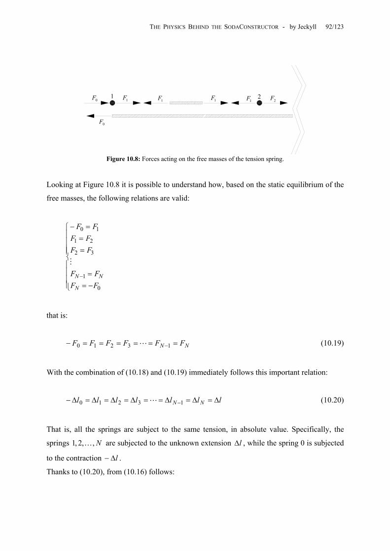
THE PHYSICS BEHIND THE SODACONSTRUCTOR - by Jeckyll 92/123
0F
0F 1F 1F 1F 1F 2F 1 2
Figure 10.8: Forces acting on the free masses of the tension spring.
Looking at Figure 10.8 it is possible to understand how, based on the static equilibrium of the
free masses, the following relations are valid:
−==
===−
−
0
1
32
21
10
FFFF
FFFF
FF
N
NN
M
that is:
(10.19) NN FFFFFF ======− −13210 L
With the combination of (10.18) and (10.19) immediately follows this important relation:
(10.20) lllllll NN ∆=∆=∆==∆=∆=∆=∆− −13210 L
That is, all the springs are subject to the same tension, in absolute value. Specifically, the
springs 1 are subjected to the unknown extension , while the spring 0 is subjected
to the contraction .
N,,2, K l∆
l∆−
Thanks to (10.20), from (10.16) follows:
THE PHYSICS BEHIND THE SODACONSTRUCTOR - by Jeckyll 93/123
(10.21)
=∆+=∆−=
Nillllll
rii
r
,,2,100
K
Substituting these relations into the equation (10.15) we get:
( ) ∑∑==
+∆=∆+=∆−N
i
ri
N
i
ri
r llNllll11
0
or better:
11
0
+
−
=∆∑=
N
lll
N
i
ri
r
(10.22)
This expression is very important, since gives us the value of the stretch of each spring in
the tension spring. From this positive value
l∆32, thanks to (10.21) it is possible to get the final
lengths of all the springs. In particular, the final length of the tension spring will be:
11
10
10
00 +
+
=+
−
−=∑∑==
N
llN
N
llll
N
i
ri
rN
i
ri
r
r (10.23)
It is very simple to verify this relation by constructing a tension spring and measuring all the
lengths at rest, as well as the final length. I will leave this exercise to you.
• The Inverse Problem
In the inverse problem, we know the final lengths l of the springs, and we
need to find lengths at rest of all the springs in our tension spring.
Nlll ,,,, 210 K
32 We can safely say this because of (10.14).

THE PHYSICS BEHIND THE SODACONSTRUCTOR - by Jeckyll 94/123
Taking into account what we have already obtained in the previous direct problem, the
solution of the inverse problem is fairly trivial. We can simply follow these three steps:
1. Choose an arbitrary value for the length at rest l . r0
2. Calculate the stretch value ∆ . 00 lll r −=
3. To calculate the length at rest of all the springs by means of the formula Nilll i
ri ,,2,1 K=∆−=
And that’s it. Once again, I will leave you with the pleasure of testing this procedure.
10.5 LINEAR MOTORS
For the last application of the quasi-static procedure, I just can’t help but examine my
beloved linear motors. These structures have given me a lot of satisfaction, so I feel obligated
to return the favor. In this last section of the last chapter of this long paper about soda physics,
I will talk about the physical-mathematical behavior of these amazing structures.
The mathematical characterization of these structures requires the study of all the possible
configurations that a linear motor can assume in its movement, so here I will limit myself to
just an explanation of the 3 point linear motor. Nevertheless, the procedure that I will adopt
for this study can also be applied to more complex linear motors.
To begin, it is important to explain how it is possible to make a 3pt linear motor. It is very
simple: a 3pt linear motor is a triangle with 3 equal muscles timed respectively at the 1/3
divisions of the wave, and simulated with maximum wave and muscle amplitudes. You can
view a 3pt linear motor here.
When the simulation is started, the triangular model will assume a typical linear configuration
and the masses will start to move back and forth with periodical cadence.
Let us start the study of this motor by taking into account the placement of the three free
masses indicated in the following Figure 10.9:

THE PHYSICS BEHIND THE SODACONSTRUCTOR - by Jeckyll 95/123
1 2 3
2x
3x
Figure 10.9: 3pt linear motor
As indicated, we will report the position of the masses with respect to mass 1. In this way, we
will eliminate from the resolution of the problem all the unessential rigid motions.
Taking into account what we know about the muscles of this motor, we can say that their
lengths at rest at a generic instant of time t will be:
( ) [ ]( ) ([( )
)]( )[ ]
π+ω+=
π+ω+=ω+=
34
13
32
23
12
sin1sin1sin1
tltltltltltl
r
r
r
(10.24)
while the effective lengths of the same three muscles at a generic instant of time t will be (see
Fig. 10.9):
(10.25)
−===
2323
313
212
xxlxlxl
Therefore, from (10.24) and (10.25) follows the stretch of the three springs:
(10.26)
−−=−=∆−=−=∆−=−=∆
rr
rr
rr
lxxllllxllllxlll
1223232323
133131313
122121212
THE PHYSICS BEHIND THE SODACONSTRUCTOR - by Jeckyll 96/123
Like in the previous problem, when the value of the stretch of the muscle , the muscle
is in extension, while when the stretch of the muscle , the muscle is in compression.
Applying Hooke’s Law, we get also the values of the tensions of the muscles:
0>∆l
0<∆l
(10.27)
∆=∆=∆=
2323
1313
1212
lkFlkFlkF
Likewise, the previous case from the equilibrium of the free masses 2 and 3 follows:
(10.28)
=+=−
00
2313
2312
FFFF
Thanks to the (10.27), this can be written as:
(10.29)
=∆+∆=∆−∆
00
2313
2312
llll
Therefore, taking into account (10.26), finally we get:
(10.30)
+=−−=−
rr
rr
llxxllxx
231323
231232
22
This is a linear system of two equations in the two unknown coordinates and . The
solution of this system of equation is:
2x 3x
( )(
++=
−+=rrr
rrr
lllxlllx
23131231
3
23131231
2
22
) (10.31)
THE PHYSICS BEHIND THE SODACONSTRUCTOR - by Jeckyll 97/123
At this point, by simply substituting the expression of the lengths at rest (10.24) in the
solution (10.31), we will get part of the solution: the laws of variation in time of the
coordinates and . ( )tx2 ( )tx3
This solution, unfortunately, isn’t enough to fully describe the behavior of the 3pt linear
motor, because the relations (10.25) are only valid when the following conditions are
satisfied:
(10.32)
>−=>=>=
000
2323
313
212
xxlxlxl
During the movement of the 3pt linear motor, the free masses continually change their
respective positions, so that the conditions (10.32) aren’t always satisfied. Therefore, the
solution provided by (10.24) and (10.31) is only valid when the configuration is like that
reported in Figure 10.9.
In order to get a general solution for the 3pt linear motor, it is indispensable to study all the
possible reciprocal positions of the three free masses during their movement. I’ve already
done this complete study but I will avoid repeating this work here. It will suffice to say that
there are a total of six possible configurations of the three free masses during their motion.
Therefore, in order to completely describe the behavior of the 3pt linear motor, we’ll need six
different solutions like (10.31).
In the diagram of Figure 10.10, I’ve reported all six different solutions. The behavior of the
coordinates and is displayed in green and red curves. It is nice to note that these
two curves were been obtained by taking different pieces of the six solutions.
( )tx2 ( )tx3
Another thing to note is that the length of period for the motion of the free masses is double
the period of the muscles.

THE PHYSICS BEHIND THE SODACONSTRUCTOR - by Jeckyll 98/123
Figure 10.10: Displacement of the masses in a 3pt linear motor.
The diagram of Figure 10.10 was been obtained by taking an initial length of the muscles
equal to and a pulsation equal to pxll 10= frmrad1=ω . The horizontal axis represents
the time expressed in frames, while the vertical axis represents the values of the displacement
and expressed in pixels. ( )tx2 ( )tx3
11. CONCLUSIONS AND ACKNOWLEDGEMENTS
The first and only thing that I wish to say in conclusion about this work is that, in the full
spirit of the sodaplay web site, I’ve done all this just for fun.
I feel obligated to give a special thanks to my friend Lectvay for his enthusiastic and patient
support of this work. Indeed, without his contribution of the revision of my text, this job
would be particularly incomprehensible. (Editor’s note: Jeckyll is too modest about his very
respectable command of English as a second language.)
Finally a special thanks goes to Ed Burton, the man who made this beautiful “piano”.

THE PHYSICS BEHIND THE SODACONSTRUCTOR - by Jeckyll 99/123
APPENDIX A: THE PENDULUM
The pendulum was the first instrument used in this paper in order to find the value of the
gravity constant g with accuracy. As you can see in Figure A.1, its structure is very simple. It
consists of an inextensible wire of negligible mass connected to a mass at a fixed point. The
system is subjected to a uniform gravitation field in the negative direction of the y-axis.
l
y
x
m x
y
α
Figure A.1: System of reference for the pendulum.
To get the differential equation of motion for the pendulum, we will apply the conservation of
energy.
The coordinates of the pendulum mass are:
(A.1) (
α−=α=cos1
sinlylx
)
therefore, their time derivatives are:
(A.2)
αα=αα=
sincos&&
&&
lylx
To find the kinetic energy we need the square of the velocity. Therefore, from (A.2) follows:

THE PHYSICS BEHIND THE SODACONSTRUCTOR - by Jeckyll 100/123
(A.3) 222 α= &lv
The total energy E of a system is given by the sum of the kinetic energy and the potential
energy. Therefore, we have:
( α−+α=+= cos122212
21 mglmlygmmvE & ) (A.4)
Since the total energy is constant in time (conservation of energy):
0=tdEd
(A.5)
Taking into account the expression (A.4) of the energy, from (A.5) follows:
0sin2221 =αα+αα= &&&& mglml
tdEd (A.6)
that is:
(A.7) 0sin2 =αω+α&&
where we have assumed the position:
lg
=ω2 (A.8)
The equation (A.7) represents the differential equation of motion for the pendulum. This
equation isn’t linear, so its solution isn’t so simple to get. In order to get a simple solution for
the above differential equation it will be necessary to assume that the maximum amplitude of
the pendulum oscillation is small enough that it be possible to approximate:

THE PHYSICS BEHIND THE SODACONSTRUCTOR - by Jeckyll 101/123
(A.9) α≈αsin
In the virtual experiments performed to find the constant g of the applet, a maximum value of
equal to has been assumed. This value certainly guarantees for the
relation (A.9) errors less than the experimental errors in the above virtual experiments.
α rad05.0max =α
Thanks to the relation (A.9), the differential equation (A.7) becomes:
0 (A.10) 2 =αω+α&&
As will be shown in detail in Appendix B, the solution of this linear differential equation is:
(A.11) ( ) ( )ϕ−ωρ=α tt cos
where:
ωαα
=ϕ
ωα
+α=ρ
0
0
202
0
tan&
&
(A.12)
and:
(A.13) ( )( )
α=αα=α
00
0
0&&
From the solution (A.11) it is possible to get the value of the period T of a complete
oscillation of the pendulum; i.e. the minimum value that satisfies the relation:
(A.14) ( ) ( )( ) tTtt ∀ϕ−+ω=ϕ−ω coscos

THE PHYSICS BEHIND THE SODACONSTRUCTOR - by Jeckyll 102/123
This value is:
ωπ
=2T (A.15)
or better:
glT π= 2 (A.16)
From this relation follows immediately:
2
24T
lg π= (A.17)
This relation is very important, because it allows us to find the value of the gravity
acceleration g by simply measuring the period T of a complete oscillation of the pendulum.
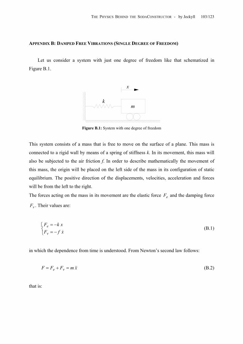
THE PHYSICS BEHIND THE SODACONSTRUCTOR - by Jeckyll 103/123
APPENDIX B: DAMPED FREE VIBRATIONS (SINGLE DEGREE OF FREEDOM)
Let us consider a system with just one degree of freedom like that schematized in
Figure B.1.
k
x
m
Figure B.1: System with one degree of freedom
This system consists of a mass that is free to move on the surface of a plane. This mass is
connected to a rigid wall by means of a spring of stiffness k. In its movement, this mass will
also be subjected to the air friction f. In order to describe mathematically the movement of
this mass, the origin will be placed on the left side of the mass in its configuration of static
equilibrium. The positive direction of the displacements, velocities, acceleration and forces
will be from the left to the right.
The forces acting on the mass in its movement are the elastic force and the damping force
. Their values are:
eF
vF
(B.1)
−=−=
xfFxkF
v
e&
in which the dependence from time is understood. From Newton’s second law follows:
(B.2) xmFFF ve &&=+=
that is:

THE PHYSICS BEHIND THE SODACONSTRUCTOR - by Jeckyll 104/123
0 (B.3) =++ xkxfxm &&&
or better:
0=++ xmkx
mfx &&& (B.4)
In order to simplify the mathematical treatment of this problem, we will assume the following
positions:
ωξ=
ω=
2
2
mfmk
(B.5)
so that the differential equation (B.4) can be written as:
0 (B.6) 2 2 =ω+ωξ+ xxx &&&
This is a linear homogeneous differential equation with constant coefficients. Its solution
provides the law of the displacement of x over time.
We are looking for solutions to the equations (B.6) in the form:
(B.7) ( ) { }tetx t λ== λ exp
The first and second derivatives of this function are:
(B.8) ( ) { }( ) { }
λλ=λλ=
ttxttx
expexp2&&
&

THE PHYSICS BEHIND THE SODACONSTRUCTOR - by Jeckyll 105/123
Therefore, substituting the relations (B.7) and (B.8) in the differential equation (B.6) we get
the equation:
(B.9) { } { } { } 0expexp2exp 22 =λω+λλωξ+λλ ttt
which is a 2nd degree algebraic equation:
(B.10) 02 22 =ω+λωξ+λ
The two solutions of this equation are:
−ξ±ξ−ω=λ 12
2,1 (B.11)
At this point, before acquiring the solutions of the original differential equation, we must
distinguish between the following three cases:
1.31.21.1
<ξ>ξ=ξ
In the firsts two cases, the values (B.11) of the constants will both be real and negative
numbers. In these two cases, the solutions of the differential problem won’t include any
oscillatory movement. The mass will tend to return directly to its quiet configuration. The
limit value of the coefficient ξ that distinguishes this particular behavior of the mass from the
typical oscillatory movement is ξ . Taking into account the positions (B.5), we have
when:
λ
1= 1=ξ
mkf 2= (B.12)
This is the value of the critical damping. Whenever the damping coefficient f is greater than
mk2 , the oscillatory behavior of the mass will vanish. These are cases of overdamping.

THE PHYSICS BEHIND THE SODACONSTRUCTOR - by Jeckyll 106/123
Taking into account the position assumed for the stiffness k and the damping coefficient f, the
relation (B.12) can also be written as:
kf 2=
Whenever we set the damping value f greater than k2 our models will not present
oscillatory behavior. I usually use overdamping when making complex models, where I need
to move free masses that are already connected out of the way in order to make other
connections. Then, I simply start the simulation of the model, and the dislocated free masses
slowly return to their places, without causing oscillations in the model.
We will not study the overdamping case, because it has no application in this paper.
Therefore, I’ll restrict myself to write just the final solution for the critical damping (B.12).
When we will have: 1=ξ
(B.13) ( ) ( )[ ] { ttvtxtx ω−+ω+= exp1 00 }
where:
(B.14) ( )( )
==
00
0
0
xvxx&
The typical behavior of a system with critical damping is reported in the diagram of
Figure B.2.

THE PHYSICS BEHIND THE SODACONSTRUCTOR - by Jeckyll 107/123
( )tx
t
Figure B.2: Displacement of a system with critical damping.
In order to define a procedure for the determination of the damping parameter f it is important
to study the third case, where . In this case, the values of the constants in (B.11) can
be written as:
1<ξ λ
ξ−±ξ−ω=λ 2
2,1 1i (B.15)
in which has been introduced the imaginary unit 1−=i . The values of the previous constant
(B.15) can be also written as:
(B.16) Diω±ωξ−=λ 2,1
in which has been introduced the damped frequency:
21 ξ−ω=ωD (B.17)
Substituting the complex values of the constant in (B.7), we get the following two
independent solutions for the differential equation (B.6):
λ
(B.18) ( ) { } { }( ) { } { }
ω−ωξ−=ωωξ−=
tittxtittx
D
D
expexpexpexp
2
1

THE PHYSICS BEHIND THE SODACONSTRUCTOR - by Jeckyll 108/123
These two solutions, thanks to the well-known Euler formula:
(B.19) { } aii sincosexp +α=α
can be also written as:
(B.20) ( ) { } ( ) ( )[ ]( ) { } ( ) ( )[
ω−ωωξ−=ω+ωωξ−=
tiitittxtiitittx
DD
DD
sincosexpsincosexp
2
1
]
One of the primary properties of a linear differential equation is that if its solution is
combined in a linear way, the result of this combination is itself a solution of the original
differential equation. Therefore, rather than use the complex solutions (B.20), it will be more
convenient to use the following two different solutions derived from (B.20) by means of two
special linear combinations:
( ) ( ) ( ) { } ( )
( ) ( ) ( ) { } (
ωωξ−=−
=
ωωξ−=+
=
tti
txtxtx
tttxtx
tx
D
D
sinexp2
cosexp2
212
211
)
)]
(B.21)
Therefore, the general solution for the linear differential equations (B.6) can be written as:
(B.22) ( ) { } ( ) ([ tAtAttx DD ω+ωωξ−= sincosexp 21
The values of the constants and can be written in terms of the following initial
conditions:
1A 2A
(B.23) ( )( )
==
00
0
0
xvxx&

THE PHYSICS BEHIND THE SODACONSTRUCTOR - by Jeckyll 109/123
After slight mathematical manipulation, we find the following values of the constants and
in terms of the initial conditions:
1A
2A
ωωξ+
=
=
D
xvA
xA00
2
01 (B.24)
so that the general solution (B.22) can be also written:
( ) { } ( ) (
ω
ωωξ+
+ωωξ−= txv
txttx DD
D sincosexp 000 ) (B.25)
Another and more compact expression for the solution (B.25) can be obtained by simply
imposing the following two positions:
000 cos;sin x
xv
D=ϕρ
ωωξ+
=ϕρ (B.26)
Indeed, substituting in (B.25) the positions (B.26) we get the following expression for the
solution of the linear differential equation (B.6):
(B.27) ( ) { } ( )ϕ−ωωξ−ρ= tttx Dcosexp
where from (B.26) follows immediately:
ωωξ+
=ϕ
ωωξ+
+=ρ
D
D
xxv
xvx
0
00
2002
0
tan
(B.28)

THE PHYSICS BEHIND THE SODACONSTRUCTOR - by Jeckyll 110/123
The solution (B.27) is particularly eloquent, because it allows us to understand the behavior of
a damped free oscillation. Indeed, this solution is essentially composed of two parts: the
amplitude of the oscillation that decreases with law , and the oscillatory part
with period equal to
{ tωξ−ρexp })( ϕ−ω tDcos Dωπ= 2T . In the following Figure B.3 it is possible to
see the typical behavior of a single degree of freedom damped free oscillation.
ν+nt nt
•
•
( )tx
t
nx
ν+nx
Figure B.3: Behavior of a damped free oscillation.
The solution (B.27) of the differential equations (B.6) is very important, because it will allow
us to find a relation for the experimental determination of the damping parameter f. By simply
measuring the amplitude of two different peaks of the oscillation, the value of the damping
parameter f can be determined.
Obviously, we will have peaks of oscillations approximately when:
(B.29) ( ) 1cos =ϕ−ω tD
This happens with periodical cadence established by the period Dωπ= 2
( ) 1=ϕ−nt
n ν+
T . Therefore, by
measuring the peak that occurs at time t such that cos , and then, after
complete oscillation, measuring the peak that occurs at time t , we
find:
nx n ωD
1≥ν ν+nx Ttn ν+=
(B.30) { }{ } ( ){ } { } {
νωξ−ωξ−ρ=ν+ωξ−ρ=ωξ−ρ=ωξ−ρ=
ν+ν+ TtTttxtx
nnnn
nn
expexpexpexpexp
}

THE PHYSICS BEHIND THE SODACONSTRUCTOR - by Jeckyll 111/123
in which the known quantities are the already measured values of and . From the
ratio of these two quantities follows:
nx ν+nx
{ }
ωπ
νωξ=νωξ=ν+ Dn
n Txx 2expexp (B.31)
Taking the natural logarithm of both sides of (B.31) we have:
Dn
n
xx
ωπ
νωξ=
ν+
2ln (B.32)
or better:
Dωπ
νωξ=δ2 (B.33)
in which has been introduced the logarithmic parameter:
=δ
ν+n
n
xx
ln (B.34)
Remembering the previous positions (B.5) and (B.17), from (B.33) follows:
2
2222
44
fmkf
−
πν=δ (B.35)
or better:

THE PHYSICS BEHIND THE SODACONSTRUCTOR - by Jeckyll 112/123
221
2
δνπ
+
=mk
f (B.36)
Thanks to (B.34) and (B.36), it is possible to experimentally determine the value of the
damping constant f.
• The Undamped Free Vibrations
In the simplest case, where the mass of Figure B.1 isn’t subjected to any air friction,
and, consequently, so that the differential equation of motion (B.6) becomes: 0=f 0=ξ
(B.37) 02 =ω+ xx&&
The general solution for this differential equation can be obtained from the solution (B.27) by
simply taking . Therefore we have: 0=ξ
(B.38) ( ) ( )ϕ−ωρ= ttx cos
where the constants ρ and are related to the initial position and velocity by means
of the relations:
ϕ 0x 0v
ω=ϕ
ω
+=ρ
0
0
202
0
tanxv
vx
(B.39)
From the solution (B.38) it is possible to see that the oscillations of this system won’t have
any diminution of their max amplitude over time. This means that in this kind of oscillation,
there isn’t any loss of energy over time. In order to create this phenomenon using the
sodaconstructor applet, simply make friction f equal to zero.

THE PHYSICS BEHIND THE SODACONSTRUCTOR - by Jeckyll 113/123
From the solution (B.38) it is also possible to see how the period T of a complete oscillation
is:
ωπ
=2T (B.40)
From this relation, taking into account the original expression of the frequency ω reported in
(B.5), follows:
2
22 4
Tmk π==ω (B.41)
or better:
mT
k2
24π= (B.42)
Thanks to this relation, by simply measuring the period of a complete oscillation of an
undamped system like that indicated in Figure B.1, it is possible to get the value of the
stiffness of a spring.

THE PHYSICS BEHIND THE SODACONSTRUCTOR - by Jeckyll 114/123
APPENDIX C: OTHERS NUMERICAL TECHNIQUES
In chapter 9, I presented the simplest numerical technique that can be used to solve a set
of differential equations: the finite difference method. Nevertheless, this technique isn’t
particularly efficient33 and can’t be applied in many cases of physical relevance. Moreover, as
can be discovered by reading an old discussion in the sodarace forum, the numerical
algorithm used in the sodaconstructor applet is the Euler method. For these reasons, I’ve
decided to explain Euler and other numerical algorithms in this appendix.
• The Euler Method: Non-Linear Differential Equation of the First Order
The most general expression for a non-linear differential equation of first order is:
(C.1) ( ) ( )[ 0,, =′ xxyxyf ]
where f is a generic function of three variables34, while is the unknown function.
Generally speaking it is possible to say that this differential equation has infinite solutions; i.e.
there are infinite functions that satisfy the equation (C.1). Nevertheless, here we are
concerned with numerical techniques that allow us to find one particular solution by means of
its numerical values. Therefore, we need to specify which of the infinite solutions of (C.1) we
are looking for. At this point the question is: how is it possible to specify what solution we are
looking for? The answer is simple: choosing a starting point from which the numerical
technique will be able to “construct” the entire solution. This starting point is normally
specified by means of the boundary condition that, for the differential equation (C.1), takes
the expression:
( )xy
( )xy
(C.2) ( ) 00 yxy =
where and are the coordinates of a particular point on the xy plane. 0x 0y
33 I’ll clarify better what I exactly mean when I speak about efficiency at the end of this appendix 34 The expression of this function is well known since it depends of the particular problem that we are studying.

THE PHYSICS BEHIND THE SODACONSTRUCTOR - by Jeckyll 115/123
It is possible to see that under certain conditions there is just one solution of the differential
equation (C.1) that will pass through the point . 00 , yx
In order to apply Euler’s method, it is important to rewrite the differential equation (C.1) in its
normal form:
(C.3) ( ) ( )[ xxyfxy ,=′ ]
)
where f is now a different function (of two variables). Obviously we also need the boundary
condition (C.2).
Since the first derivative of a function represents the slope of that function at a particular
point, we are immediately able to recognize that the differential equations (C.3) together with
its boundary condition (C.2) give us the slope “s” of the unknown function at the point
(see Figure C.1):
( )xy
00 , yx
(C.4) ( ) ( )[ ] ( 000000 ,, xyfxxyfxys ==′=
x
y
0x hxx += 01
h
0y
1y
( )1xy ( )hxyhs 00 ′=
( )xy
Figure C.1: The geometric meaning of the first derivative
Therefore, if we choose a finite interval h, we’ll be able to get a second point on our unknown
function taking:
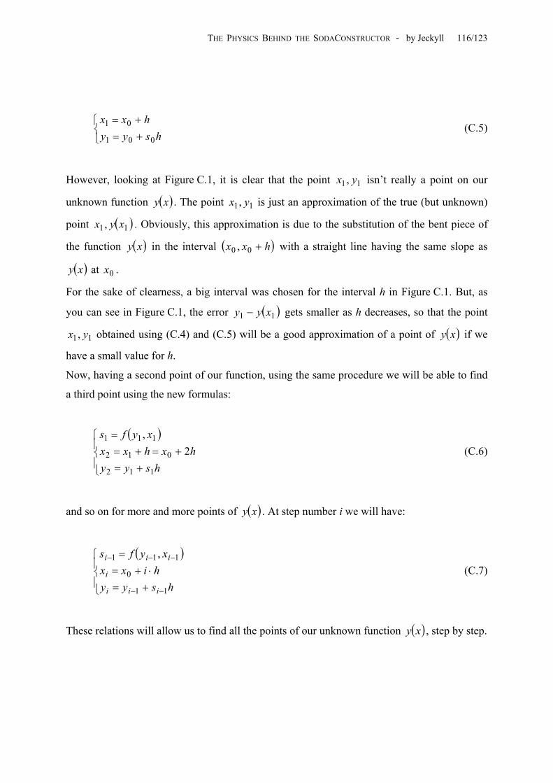
THE PHYSICS BEHIND THE SODACONSTRUCTOR - by Jeckyll 116/123
(C.5)
+=+=
hsyyhxx
001
01
However, looking at Figure C.1, it is clear that the point isn’t really a point on our
unknown function . The point is just an approximation of the true (but unknown)
point . Obviously, this approximation is due to the substitution of the bent piece of
the function in the interval ( with a straight line having the same slope as
at .
11, yx
( )xy 11, yx
xx 00 ,
( 11, xyx
y
0x
))( )x h+
( )xy
For the sake of clearness, a big interval was chosen for the interval h in Figure C.1. But, as
you can see in Figure C.1, the error gets smaller as h decreases, so that the point
obtained using (C.4) and (C.5) will be a good approximation of a point of if we
have a small value for h.
( )11 xyy −
11, yx ( )xy
Now, having a second point of our function, using the same procedure we will be able to find
a third point using the new formulas:
(C.6) ( )
+=+=+=
=
hsyyhxhxx
xyfs
112
012
111
2,
and so on for more and more points of . At step number i we will have: ( )xy
(C.7) ( )
+=⋅+=
=
−−
−−−
hsyyhixx
xyfs
iii
i
iii
11
0
111 ,
These relations will allow us to find all the points of our unknown function , step by step. ( )xy

THE PHYSICS BEHIND THE SODACONSTRUCTOR - by Jeckyll 117/123
• The Euler Method: System of Non-Linear Differential Equations of the First Order
In the previous section I talked about the use of Euler’s method when our mathematical
problem is represented by a non-linear differential equation of the first order. Here I’ll talk
about the use of the same numerical algorithm when our problem is represented by a system
of non-linear differential equations of the first order.
Since it is trivial to get the generalization to a system of N differential equations, here I’ll
restrict myself to talk about a simple system of two differential equations of first order in two
unknown functions. This system in its normal form is:
(C.8) ( ) ( ) ( )[ ]( ) ( ) ( )[
=′=′
xxzxygxzxxzxyfxy
,,,,]
where and are the unknown functions while f and g are two generic functions with
three variables
( )xy ( )xz35. Obvioulsy, along with this system of differential equations we must also
specify the correspondent boundary conditions. These, for our problem, are:
(C.9) ( )( )
==
00
00
zxzyxy
Like in the previous case, taking into account the geometrical meaning of the first derivative
of a function, from (C.8) and (C.9) we get the slopes and of the functions and
respectively in correspondence with the abscissa :
ys0
0x
zs0 ( )xy
( )xz
(C.10) ( )( )
==
xzygsxzyfs
z
y
,,,,
000
000
35 As in the previous case, these functions are well known since they depend on the particular problem that we are studying.

THE PHYSICS BEHIND THE SODACONSTRUCTOR - by Jeckyll 118/123
Therefore, fixing a small finite interval h, the approximate values of the functions and
in correspondence with the abscissa will be:
( )xy
( )xz hx +0
(C.11)
+=+=
hszzhsyy
z
y
001
001
Thanks to these new values we will be able to iterate the same procedure in order to get a
sequence of points that represents our approximate solution to the problem defined
by the system of differential equations (C.8) and the relative boundary conditions (C.9).
iii zyx ,,
The generic expressions for step number i of the iteration are:
(C.12) ( )(
+=+=
==
⋅+=
−−
−−
−−−−
−−−−
hszzhsyy
xzygsxzyfs
hixx
ziii
yiii
iiizi
iiiyi
i
11
11
1111
1111
0
,,,,
)
]
• The Euler Method: Non-Linear Differential Equations of the Second Order
Usually, the equations of motion for a physical system are expressed in terms of
differential equations of the second order. For this reason we will now discuss the application
of the Euler method in the resolution of a non-linear differential equation of the second order.
This equation in its normal form has the expression:
(C.13) ( ) ( ) ( )[ xxyxyfxy ,,′=′′
where is the unknown function and f is a particular function with three variables. ( )xy
Once again, you can see that in order to get a specific solution of this differential equation
(C.13) we need an appropriate number of boundary conditions. In this case we have:

THE PHYSICS BEHIND THE SODACONSTRUCTOR - by Jeckyll 119/123
(C.14) ( )( )
′=′=
00
00
yxyyxy
with the constants . 000 ,, yyx ′
As we know, Euler’s method is based on the geometric meaning of the first derivative of a
function, so this method seemingly can’t be applied to the differential equation (C.13), where
the second derivative of the function appears. However, I’ll show you how it is always
possible to transform a differential equation of the second order (C.13) into a system of two
differential equations of the first order. To do that, let’s examine the following position:
( )xy
(C.15) ( ) ( )xyxz ′=
Indeed, using this relation, the differential problem defined by the relations (C.13) and (C.14)
becomes:
(C.16) ( ) ( )( ) ( ) ( )[
=′=′
xxyxzfxzxzxy
,, ]
together with the following boundary conditions:
(C.17) ( )( )
′==
00
00
yxzyxy
It’s easy to recognize that the differential problem shown in equations (C.16) and (C.17) is an
instance of the problem that wediscussed in the previous section. Therefore, the Euler method
is applicable.

THE PHYSICS BEHIND THE SODACONSTRUCTOR - by Jeckyll 120/123
• The Euler Method: Systems of Differential Equations of the Second Order
The equations of the motion of a generic model were formulated in chapter 8 of this
paper. Looking at (8.10) it is easy to see that these equations are organized in a system of 2N
non-linear equations of second order in 2N unknown functions of time. How can these
equations be solved with Euler’s method? The answer is contained in the previous three
sections of this appendix. Indeed, using the same mathematical trick used in the previous
section, it is easy to understand how the equations (8.10) can be transformed into a system of
4N differential equations of the first order in 4N unknown functions of time. These unknown
functions will be the nodes’ coordinates of the model and the relative components of velocity.
Therefore, the resolution of the equations (8.10) can easily be obtained using the Euler
method, as already explained.
• The Euler Method: Final Considerations
Even if the Euler method is better than the finite differences method explained in
chapter 9, it still isn’t particularly efficient. But what exactly does it mean to say that a
numerical method isn’t “efficient”? The question is perfectly sensible.
Obviously, before we can say that a particular numerical technique isn’t efficient, we need
another numerical technique to compare it to. So it would be more correct to state that the
Euler method isn’t as efficient as other numerical methods. But saying shifts the problem.
Now the question is: what exactly is meant by the word “efficiency”? The answer isn’t trivial
for the simple reason that the concept of “efficiency” depends greatly on the purpose of our
use of a numerical technique.
Usually the concept of efficiency of a numerical method is strictly related to both the accuracy
of the results and the speed of calculus. Depending on our particular purpose, it could
sometimes be necessary to compromise either the accuracy of the results or the speed of the
calculus. Moreover, for certain kinds of calculus under the category of “simulations”, the
purposes are both accuracy of results and speed of calculus; but this isn’t an iron rule. Indeed,
although the sodaconstructor is essentially a simulation program, it is important to remember
that it is also just a game36, so it isn’t particularly important to obtain perfect accuracy of the
36 A beautiful game in my opinion.

THE PHYSICS BEHIND THE SODACONSTRUCTOR - by Jeckyll 121/123
results. It is enough that the models can walk reliably on the screen. Therefore, for the
sodaconstructor, it might be better to favor the speed of calculus.
The Euler method isn’t particularly efficient with either accuracy or speed. Still, this method
is good enough for the sodaconstructor’s purposes37.
The last question is: what numerical methods are better than Euler?
• The Runge-Kutta’s Algorithm
Here I wish to say just a few words about the Runge Kutta algorithm. The main reason is
that this algorithm was used in another simulation game similar to the sodaconstructor but in
3D: Beaker’s Springs Lab.
The first important thing to say is that the Runge-Kutta algorithm is based on the Euler
method. Also, the Runge-Kutta algorithm represents a class of numerical techniques. For this
reason, here I’ll talk only about the first order Runge-Kutta method38.
The problem that we’ll take into consideration is defined by the following non-linear
differential equation of the first order in normal form:
(C.18) ( ) ( )[ xxyfxy ,=′ ]
)
together with the boundary condition:
(C.19) ( ) 00 yxy =
The basic idea of the Runge-Kutta first order method is to use a different slope in order to get
a more accurate value of the approximate value . In the Euler method the value of the slope
was:
1y
(C.20) ( ) ( 0000 , xyfxys =′=
37 i.e. our entairtment. 38 The zero order Runge-Kutta method is just the Euler method.

THE PHYSICS BEHIND THE SODACONSTRUCTOR - by Jeckyll 122/123
In the Runge Kutta method, however, the value of the slope is taken in the middle of the
interval . As can be seen in Figure C.2, the value of this slope is taken at the
coordinates
( hxx +00 , )
hsy 021
0 +hx 21
0 ,+
0~s
where is the value defined by (C.20). This new and more
accurate slope is given by (C.18) by means of the relation:
0s
( ) ( )hxhsyfhxys 21
0021
021
00 ,~ ++≅+′= (C.21)
0x hx 21
0 + hxx += 01
0y
1y
( )1xy
ey1
x
y
hsy 021
0 +
( )xy
Figure C.2: The Runge-Kutta’s method.
Therefore the approximate value of the function in correspondence with the abscissa
is given by:
( )xy
hxx += 01
(C.22) hsyy 001~+=
It is clear from Figure C.2 that this approximate value is more accurate than the corresponding
value of the Euler method. ey1
At this point, it is possible to find the sequence of points of our unknown function by
simply iterating the above procedure.
( )xy
The generic formulas for step number i of the above procedure are the following:

THE PHYSICS BEHIND THE SODACONSTRUCTOR - by Jeckyll 123/123
( )(
+=++=
=+=
−−
−−−−
−−−
hsyyhxhsyfs
xyfshixx
iii
iiii
iii
i
11
21
1121
11
111
0
~,~
,) (C.23)
It is possible to use the Runge-Kutta first order method for different objectives. The first
possibility is to use this numerical method in order to obtain an approximate solution more
accurate than the solution obtained using the Euler method, while still maintaining the same
computational charge. Or, a second possibility is to use this method in order to get an
approximate solution as accurate as the solution obtained using the Euler method, but having
a smaller computational charge.