Forecasting Agricultural Commodity Prices Using Multivariate Bayesian Machine Learning

RegressionRegression

by

Andres M. Ticlavilca, Dillon M. Feuz, and Mac McKee

Suggested citation format:Suggested citation format:

Ticlavilca, A. M., Dillon M. Feuz and Mac McKee. 2010. “Forecasting Agricultural Commodity Prices Using Multivariate Bayesian Machine Learning Regression.” Proceedings of the NCCC-134 Conference on Applied Commodity Price Analysis, Forecasting, and Market Risk Management. St. Louis, MO. [http://www.farmdoc.illinois.edu/nccc134].

Forecasting Agricultural Commodity Prices Using Multivariate Bayesian Machine

Learning Regression

Andres M. Ticlavilca,

Dillon M. Feuz,

and

Mac McKee *

Paper presented at the NCCC-134 Conference on Applied Commodity Price Analysis, Forecasting, and Market Risk Management

St. Louis, Missouri, April 19-20,2010

Copyright 2010 by Andres M. Ticlavilca, Dillon M. Feuz and Mac McKee. All rights reserved. Readers may verbatim copies of this document for non-commercial purposes by any means,

provided that this copyright notice appears on all such copies.

* Andres M. Ticlavilca (andres.t@aggiemail.usu.edu) is a Graduate Research Assistant at the Utah Water Research Laboratory, Department of Civil and Environmental Engineering, Utah State University. Dillon M. Feuz (dillon.feuz@usu.edu) is a Professor at Utah State University in the Applied Economics Department. Mac McKee (mac.mckee@usu.edu) is the Director of the Utah Water Research Laboratory and Professor at the Department of Civil and Environmental Engineering, Utah State University.

1

Forecasting Agricultural Commodity Prices Using Multivariate Bayesian Machine Learning Regression

The purpose of this paper is to perform multiple predictions for agricultural commodity prices (one, two and three month periods ahead). In order to obtain multiple-time-ahead predictions, this paper applies the Multivariate Relevance Vector Machine (MVRVM) that is based on a Bayesian learning machine approach for regression. The performance of the MVRVM model is compared with the performance of another multiple output model such as Artificial Neural Network (ANN). Bootstrapping methodology is applied to analyze robustness of the MVRVM and ANN. Keywords: Commodity prices, Forecasting, Machine learning, Bayesian

Introduction

The last few years there has been an increase in the volatility of many agricultural commodity prices. This has increased the risk faced by agricultural producers. The main purpose of agricultural commodity price forecasting is to allow producers to make better-informed decisions and to manage price risk. Simple price forecast models such as naïve, or distributed-lag models have performed quite well in predicting agricultural commodity prices (Hudson, 2007). Other models such as “deferred future plus historical basis” models (Kastens et al., 1998), autoregressive integrated moving average (ARIMA) models and composite models (Tomek and Myers, 1993) lead to more accurate estimates. However, as the accuracy increases, so does the statistical complexity (Hudson, 2007). Practical applications of more complex models are limited by the lack of required data and the expense of data acquisition. On the other hand, the increased volatility in agricultural commodity prices may increase the difficulty of forecasting accurately making the simple methods less reliable and even the more complex forecast methods may not be robust in this new market environment. To overcome these limitations, machine learning (ML) models can be used as an alternative to complex forecast models. ML theory is related to pattern recognition and statistical inference wherein a model is capable of learning to improve its performance on the basis of its own prior experience (Mjolsness and DeCoste, 2001). Examples of ML models include the artificial neural networks (ANNs), support vector machines (SVMs) and relevance vector machines (RVMs). ML models have been applied in financial economics modeling. Enke and Thawornwong (2005) used data mining and ANNs to forecast stock market returns. Co and Boosarawongse (2007) demonstrated that ANNs outperformed exponential smoothing and ARIMA models in forecasting rice exports. Also ML models have been applied in forecasting agricultural commodity prices. Shahwan and Odening (2007) used a hybrid between ANNs and ARIMA model to predict agricultural commodity prices.

2

The paper reported here presents a ML model to perform monthly multi-step-ahead predictions with predictive confidence intervals for agricultural commodity prices. Therefore, the model recognizes the patterns between multivariate outputs (future commodity prices) and multivariate inputs (past data collected about commodity prices).

This paper applies the Multivariate Relevance Vector Machine (MVRVM) (Thayananthan, 2005; Thayananthan et al., 2008). The MVRVM is an extension of the RVM algorithm developed by Tipping and Faul (2003). It can be used to produce multivariate outputs with confidence interval, via its Bayesian approach. The MVRVM has the same capabilities of the conventional RVM: high prediction accuracy, robustness, and characterization of uncertainty in the predictions.

The remainder of the paper describes the MVRVM approach, the model application for agricultural commodity price forecast, a comparison with an ANN model and conclusions.

Model Description The MVRVM was developed by Thayananthan (2005) to provide an extension of the RVM algorithm for regression (Tipping, 2001; Tipping and Faul, 2003) to multivariate outputs. Given a set of training examples of input-target vector pairs {x(n), t(n)} N

1n , where Ν is the number of pattern observations, x Є RD is a input vector, t Є RM is a output target vector, the model learns the dependency between input and output target with the purpose of making accurate predictions of t for previous values of x:

t = W Φ(x) + ε (1) where W is a M x P weight matrix and P = N+1. The error ε is assumed to be zero-mean Gaussian with diagonal covariance matrix S=diag(σ1

2, …, σM2).

Φ(x) is a vector of basis functions of the form Φ(x) = [1, K(x,x(1),… K(x,x(N))), where K(x,xn) is a kernel function (Tipping, 2001, Thayananthan, 2008). In this paper, we considered a Gaussian kernel K(x,xn) = exp(-r-2||x- x(n)||2) where r is the kernel width parameter. A likelihood distribution of the weights is defined as a product of Gaussians of the weight vectors (wr) corresponding to each output target (τr) (Thayananthan, 2008):

N

1n

M

1r

2rrr

(n)(n)N1n

(n) )σ,|()),(|()|}p({ ΦwτSxWtSW,t Φ (2)

where Φ = [1, Φ(x1), Φ(x2),..., Φ(xN)]. To avoid overfitting from Equation (2), Tipping (2001) proposed constraining the selection of parameters by applying a Bayesian approach and defining an explicit zero-mean Gaussian prior probability distribution over the weights (Thayananthan, 2008):

3

M

1r

P

1j

M

1rr

2jrj )0,|()α0,|(w )|p( AwAW (3)

where A = diag(α1

-2, …, αP-2)T is a diagonal matrix of hyperparameters αj, and wrj is the (r,j)th

element of the weight matrix W. Each αj controls the strength of the prior over its associated weight (Tipping and Faul, 2003). The posterior distribution of the weights is proportional to the product of the likelihood and prior distributions:

)p( )|}p({ )}{|p( N

1nN

1n A|WSW,tAS,,tW (4) Then, this posterior parameter distribution can be defined as the product of Gaussians for the weight vectors of each target (Thayananthan, 2008):

M

1rrrr

N1n

N1n ),|()p( )|}p({ )}{|p( ΣµwA|WSW,tAS,,tW (5)

with covariance and mean, Σr = (A + σr

-2 ΦT Φ)-1 and µr = σr-2 Σr ΦT τr, respectively.

An optimal weight matrix can be obtained by estimating a set of hyperparameters that maximizes the data likelihood over the weights in Equation (5) (Thayananthan, 2008). The marginal likelihood is then:

, WA|WSW,tSA,|t )dp( )|}p({ )}p({ N1n

N1n

)21(exp|| )()σΦ,|( r

1-r

Tr

21M

1rr

2rr

M

1rr τHτHA0,|wwτ

(6)

where Hr = σr

2I + Φ A-1ΦT . The optimal set of hyperparameters αopt = P1j

optj }{ α and noise

parameters (σopt )2 = M1r

optr }{σ are obtained by maximizing the marginal likelihood using the fast

marginal likelihood maximization algorithm proposed by Tipping and Faul (2003). Many elements of α go to infinity during the optimization process, for which the posterior probability of the weight becomes zero. These nonzero weights are called the relevance vectors (RVs) (Tipping and Faul, 2003). Then, we can obtain the optimal covariance Σopt = M

1roptr }{ Σ and mean µopt = M

1roptr }{ µ .

Given a new input x*, we can compute the predictive distribution for the corresponding output target t* (Tipping, 2001) :

WσαtWσWtσαtt d))(,,|.p())(,|*p(=))(,,|*p( 2optopt2opt2optopt (7)

4

In Equation (7), both terms in the integrand are Gaussian. Then, this equation can be computed as:

)*)(*,|*())(,,|*p( 22optopt σytσαtt (8)

where y*=[ y1*,..., yr*,... yM*]T is the predictive mean with yr* = (µr

opt)TΦ(x*); and (σ*)2 = [(σ1*)2,... (σr*)2,..., (σM*)2]T is the predictive variance with (σr*)2= (σr

opt)2 + Φ(x*)T Σropt

Φ(x*) which contains the sum of two variance terms: the noise on the data and the uncertainty in the prediction of the weight parameters (Tipping, 2001). The standard deviation σr* of the predictive distribution is defined as a predictive error bar of yr* (Bishop 1995). Then, the width of the 90% Bayesian confidence interval for any yr* can be ± 1.65.σr*. This Bayesian confidence interval (which is based on probabilistic approach) should not be confused with a classical frequentist confidence interval (which is based on the data).

Data

Monthly data for cattle, hog and corn prices were obtained for 21 years. The data were obtained from the Livestock Marketing Information Center website www.lmic.info and the data are initially collected and reported by the USDA-AMS. Corn prices were from Omaha, NE market; cattle prices were from Nebraska live fed cattle market, and hog prices were from the Iowa/southern Minnesota market. These are all large markets that are frequently used as standards by which to judge other markets. Procedures

Monthly data from 1989 to 2003 were used to train each model and estimate the model parameters. Monthly data from 2004 to 2009 were used to test the models.

The inputs used in the model to predict monthly commodity price are expressed as x = [xtp-m] T (9)

where, tp = time of prediction m = number of months previous to the prediction time x1tp-m = Commodity price ‘m’ months previous to the prediction time

The multiple output target vector of the model is expressed as t = [ ttp+1, ttp+2 , ttp+3]T (10)

where, ttp+1 = prediction of commodity price one month ahead ttp+2 = prediction of commodity price two months ahead ttp+3 = prediction of commodity price three months ahead

5

Performance evaluation

The kernel width is a smoothing parameter which defines a basis function to capture patterns in the data. This parameter cannot be estimated with the Bayesian approach. For this paper, a sensitivity analysis is performed to estimate the kernel width that gives accurate test results. The statistics used for the selection of the model is the root mean square percentage error (RMSPE), and is given by:

100.t

*ttN1RMSPE

N

1i

2

(11)

where t is the observed output; t* is the predicted output and N is the number of observations. The sensitivity analysis was done by building several MVRVM models with variation in the kernel width (from 1 to 60) and the number of previous months required as input (from 1 to 12 months). The selected model was the one with the minimum RMSPE of the average outputs corresponding to the testing phase.

Bootstrap analysis

The bootstrap method (Efron and Tibshirani,1998) was used to guarantee robustness of the MVRVM (Khalil et al., 2005a). The bootstrap data set was created by randomly selecting from the whole training data set, with replacement. This selection process was independently repeated 1,000 times to yield 1,000 bootstrap training data sets, which are treated as independent sets (Duda et al., 2001). For each of the bootstrap training data sets, a model was built and evaluated over the original test data set. A robust model is one that shows a narrow confidence bounds in the bootstrap histogram (Khalil et al., 2005b). A narrow confidence bounds implies low variability of the statistics with future changes in the nature of the input data, which indicates that the model is robust.

Comparison between MVRVM and ANN

A comparative analysis between the developed MVRVM and ANNs is performed in terms of performance and robustness. Readers interested in greater detail regarding ANN and its training functions are referred to Demuth et al. (2009). Several feed-forward ANN models were trained and tested with variation in the type of training function, size of layer(from 1 to 10) and the number of months previous to the prediction time (from 1 to 12 months). The selected model was the one with the minimum RMSPE of the average outputs corresponding to the testing phase.

6

Results and Discussions

Table 1 shows the selected kernel width and the number of input months for each commodity price forecasting. The selected models were the ones with the lowest RMSPE of the average results. Table 1 Selected MVRVM for each commodity (testing phase)

1-month 2-months 3-monthsCorn 2 26 6.0 9.7 13.2 9.6Cattle 8 14 3.1 5.0 6.3 4.8Hog 11 32 6.1 7.8 9.6 7.8

RMSPE (%) Average RMSPE (%)

Number of previous months

Kernel width

Figures 1-3 show the predicted outputs (full lines) of the MVRVM for the testing phase for corn, cattle and hog prices respectively. These figures also show the 0.90 Bayesian confidence interval (shaded region) associated with the predictive variance (σr*)2 of the MVRVM in Equation (8). We can see that this Bayesian confidence interval appears to be unchanged during the whole test period. As we mentioned in section 2, the predictive variance is (σr*)2= (σr

opt)2 + Φ(x*)T Σropt

Φ(x*). The first term depends on the noise on the training data and the second term depends on the prediction of the parameter when a new input x* is given. From our results, it was found that there is a significant contribution from the first term (the noise variance on the training data) which made the contribution from the second term very small (close to zero). That is why the width of the confidence interval for the test results appears to be almost constant. The model learns the patterns for one and two months ahead for the three commodities (Figures 1a, 1b, 2a, 2b, 3a and 3b). The performance accuracy is reduced for the three-month ahead price prediction of the three commodities (Figures 1c, 2c and 3c). This accuracy reduction is found in most of the multiple-time-ahead prediction models, where the farther we predict into the future, the less accurate the prediction becomes. Also, we can see that the model performance decreases in early 2008 for the corn price predictions. As we mentioned in section 4, monthly data from 1989 to 2003 were used to train the model and estimate the model parameters. The model probably needs to be retrained at this period (early 2008) and also it may need more number of previous months as inputs data during this period. However, we prefer not to provide more definite conclusions, as they might not be sufficiently well supported. More detailed analysis regarding strategies to improve model performance will be carried out for future research.

7

Figure 1. Observed versus predicted monthly corn price of the MVRVM model with 0.90 Bayesian confidence intervals (shaded region) for the testing phase: (a) 1-month ahead, (b) 2-months ahead, (c) 3-months ahead

8

Figure 2. Observed versus predicted monthly cattle price of the MVRVM model with 0.90 Bayesian confidence intervals (shaded region) for the testing phase: (a) 1-month ahead, (b) 2-months ahead, (c) 3-months ahead

9

Figure 3. Observed versus predicted monthly hog price of the MVRVM model with 0.90 Bayesian confidence intervals (shaded region) for the testing phase: (a) 1-month ahead, (b) 2-months ahead, (c) 3-months ahead

10

Table 2 shows the selected ANN models for two types of training function. The model with conjugated-gradient-training function shows the lowest RMSPE of the average results for corn. The model with resilient-backpropagation-training function shows the lowest RMSPE of the average results for cattle and hog. Therefore they were selected as the best type of training function for each model that describes the input-output patterns. Table 2. Selected ANN models for two types of training function (testing phase)

Type of training function 1-month 2-months 3-months 1-month 2-months 3-months 1-month 2-months 3-months Corn Cattle HogResilient backpropagation 8.2 10.4 12.9 3.6 5.4 6.8 6.5 7.8 9.8 10.5 5.3 8.0Conjugate gradient with Powell-Beale restarts 7.2 9.3 11.8 3.5 5.5 7.1 6.2 8.6 10.3 9.5 5.4 8.4

Average RMSPE (%)RMSPE (%)

Corn Cattle Hog

Table 3 shows the selected size of layer and the number of input months for each commodity price forecasting for the ANN models. Table 3. Selected ANN for each commodity price prediction (testing phase).

1-month 2-months 3-monthsCorn 10 2 7.2 9.3 11.8 9.5Cattle 4 1 3.6 5.4 6.8 5.3Hog 8 4 6.5 7.8 9.8 8.0

Number of previous months

Size of layer

RMSPE (%) Average RMSPE (%)

11

Figure 4. Observed versus predicted monthly corn price of the ANN model for the testing phase: (a) 1-month ahead, (b) 2-months ahead, (c) 3-months ahead

12

Figure 5. Observed versus predicted monthly cattle price of the ANN model for the testing phase: (a) 1-month ahead, (b) 2-months ahead, (c) 3-months ahead

13

Figure 6. Observed versus predicted monthly hog price of the ANN model for the testing phase: (a) 1-month ahead, (b) 2-months ahead, (c) 3-months ahead

14

Figures 4-6 show the observed (dots) and predicted (full lines) outputs of the ANN for the testing phase for corn, cattle and hog prices respectively. RMSPE and RMSE statistics for the MVRVM and ANN prediction performance are displayed in Table 4. We can see that the MVRVM outperforms, has a smaller forecast error, the ANN for corn price prediction one month ahead, cattle price prediction one, two and three months ahead, and hog price prediction one and three months ahead. On the other hand, ANN outperforms MVRVM for corn price prediction two and three months ahead. Hog price predictions for two months ahead are similar for both models. The ANN cattle model (Figure 5) appears to be shifted with a 1-3 month lag. This ANN model may need more number of previous months as inputs data during this period. On the other hand, the MVRVM cattle model (Figure 2) can overcome the performance lag problems since its Bayesian approach allows us to calculate predictive confidence intervals , instead of just providing a single target output (Bishop 1995) such as is the ANN model results. Table 4. Model Performance using RMSPE and RMSE (testing phase)

Model Statistics 1-month 2-months 3-months 1-month 2-months 3-months 1-month 2-months 3-monthsMVRVM RMSPE (%) 6.0 9.7 13.2 3.1 5.0 6.3 6.1 7.8 9.6

RMSE ($) 0.22 0.36 0.52 2.74 4.43 5.63 4.07 5.36 6.41ANN RMSPE (%) 7.2 9.3 11.8 3.6 5.4 6.8 6.5 7.8 9.8

RMSE ($) 0.26 0.33 0.45 3.19 4.70 6.03 4.23 5.31 6.29

Corn Cattle Hog

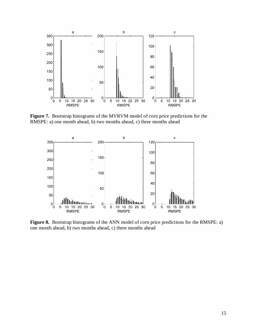
Figures 7-12 show the bootstrap histograms for the RMSE test based on 1,000 bootstrap training data sets of the MVRVM and ANN models for corn, cattle and hog prices respectively. The bootstrapped histograms of the MVRVM models (Figures 7, 9 and 11) show narrow confidence bounds in comparison to the histograms of the ANN models (Figures 8, 10 and 12). Therefore, the MVRVM is more robust.

15

Figure 7. Bootstrap histograms of the MVRVM model of corn price predictions for the RMSPE: a) one month ahead, b) two months ahead, c) three months ahead

Figure 8. Bootstrap histograms of the ANN model of corn price predictions for the RMSPE: a) one month ahead, b) two months ahead, c) three months ahead

16

Figure 9. Bootstrap histograms of the MVRVM model of cattle price predictions for the RMSPE: a) one month ahead, b) two months ahead, c) three months ahead

Figure 10. Bootstrap histograms of the ANN model of cattle price predictions for the RMSPE: a) one month ahead, b) two months ahead, c) three months ahead

17

Figure 11. Bootstrap histograms of the MVRVM model of hog price predictions for the RMSPE: a) one month ahead, b) two months ahead, c) three months ahead

Figure 12. Bootstrap histograms of the ANN model of hog price predictions for the RMSPE: a) one month ahead, b) two months ahead, c) three months ahead

18

Summary and Conclusions This paper applies a MVRVM model to develop multiple-time-ahead predictions with confidence intervals of monthly agricultural commodity prices. The predictions are one, two and three months ahead of prices of cattle, hogs and corn. The MVRVM is a regression tool extension of the RVM model to produce multivariate outputs. The statistical test results indicate an overall good performance of the model for one and two month’s prediction for all the commodity prices. The model performance decreased in early 2008 for the corn price predictions. The performance also decreased for the three-month prediction of the three commodity prices. The MVRVM model outperforms the ANN most of the time with the exception of corn price prediction two and three months ahead. However, the bootstrap histograms of the MVRVM model show narrow confidence bounds in comparison to the histograms of the ANN model for the three commodity price forecasts. Therefore, the MVRVM is more robust. The results presented in this paper have demonstrated the overall good performance and robustness of MVRVM for simultaneous multiple-time-ahead predictions of agricultural commodity prices . The potential benefit of these predictions lies in assisting producers in making better-informed decisions and managing price risk. Future work In this research, we have not analyzed the sparse property (low complexity) of the MVRVM since we have worked with relatively small data set (166 monthly observations) to train the model. Future research will be performed by analyzing weekly price (more than 1000 observations) and fully exploit the sparse characteristics of the Bayesian approach when dealing with large dataset. Also, the relevance vectors (RVs) (which are related to the sparse property) are the summary of the most essential observations of the training data set to build the MVRVM. In this paper we have not analyzed the RVs since we are dealing with small data set. Future research will be performed by analyzing with more details the statistical meaning of RVs with respect to a large training data set. For example, this analysis can also be related to whether we would recommend reducing the number of historical data observations for retraining the model with new data in the future. The kernel width and the number of previous months required as input cannot be estimated with the Bayesian approach. For this paper, a sensitivity analysis (by trial and error) was performed to estimate these parameters that gave accurate test results. We could see that the overall test results are good. However, the model performance decreases for some periods ( i.e. early 2008 for the corn price predictions). Therefore, more analysis regarding the selection of these parameters (kernel width an number of previous months as inputs) will be carried out in a follow-up paper.

19

Application of a hybrid model (e.g. Bayesian approach embedded in ANN model) will be applied and compared to the MVRVM model in terms of accuracy, complexity and robustness.

References

Bishop, C. M. Neural Networks for Pattern Recognition (1995). Oxford University Press UK. Co, H. C., and R. Boosarawongse (2007). “Forecasting Thailand’s Rice Export: Statistical Techniques vs. Artificial Neural Networks.” Computers and Industrial Engineering 53: 610-627. Demuth, H., M. Beale, and M. Hagan (2009) Neural network toolbox user’s guide, The MathWorks Inc, MA, USA. Duda, R. O., P. Hart and D. Stork (2001). Pattern Classification, edited by Wiley Interscience, Second Edition, New York. Efron, B., and R. Tibshirani (1998) An introduction of the Bootstrap. Monographs on Statistics and Applied Probability 57, CRC Press LLC, USA. Enke, D. and S. Thawornwong (2005). The Use of Data Mining and Neural Networks for Forecasting Stock Market Returns. Expert Systems with Applications 29:927-940. Hudson, D. (2007). Agricultural Markets and Prices, Maden, MA. Blackwell Publishing. Kastens, T. L., R. Jones and T. C. Schroeder (1998). Future-Based Price Forecast for Agricultural Producers and Businesses. Journal of Agicultural and Resource Economics 23(1): 294-307. Khalil, A., M. McKee, M. W. Kemblowski, and T. Asefa (2005a). Sparse Bayesian learning machine for real-time management of reservoir releases. Water Resources Research, 41, W11401, doi: 10.1029/2004WR003891. Khalil, A., M. McKee, M. W. Kemblowski, T. Asefa, and L. Bastidas (2005b). Multiobjective analysis of chaotic dynamic systems with sparse learning machines, Advances in Water Resources, 29, 72-88, doi:10.1016/j.advwatres.2005.05.011. Mjolsness, E., and D.DeCoste (2001). Machine learning for science: state of the art and future prospects. Science 293:2051–2055. Shahwan, T and M Odening (2007). Forecasting Agricultural Commodity Prices using Hybrid Neural Networks. In Computational Intelligence in Economics and Finance. Springer, Berlin. 63-74. Thayananthan, A. (2005). Template-based Pose Estimation and Tracking of 3D Hand Motion. PhD Thesis, Department of Engineering, University of Cambridge, Cambridge, United Kingdom.

20

Thayananthan, A., R. Navaratnam, B. Stenger, P.H.S. Torr, and R. Cipolla (2008). Pose estimation and tracking using multivariate regression, Pattern Recognition Letters 29(9), pp. 1302-1310. Tipping, M. E. (2001), Sparse Bayesian learning and the relevance vector machine, Journal of Machine Learning, 1, 211–244. Tipping, M., and A. Faul (2003). Fast marginal likelihood maximization for sparse Bayesian models, paper presented at Ninth International Workshop on Artificial Intelligence and Statistics, Soc. for Artif Intel and Stat, Key West, Florida. Tomek, W. G., and R. J. Myers (1993). Empirical Analysis of Agricultural Commodity Prices: A Viewpoint, Review of Agricultural Economics, 15(1):181-202.