11/10/2008 1

Berkeley Water Center

Data Cube-Matlab Interface

User Manual

11/10/2008 2

CONTENTS

Overview ......................................................................................................................... 3

An introduction to Berkeley Water Center data cubes ................................................... 3

Installation ...................................................................................................................... 4

Add library to Matlab Path ......................................................................................... 5

Adding java classes to classpath ................................................................................. 5

Result Data Structure ...................................................................................................... 6

Example data structure usage ...................................................................................... 6

Using the Graphical User Interface ................................................................................ 7

Starting the interface ................................................................................................... 7

Query dialog description and usage ............................................................................ 9

Dimensions ........................................................................................................... 10

Measure ................................................................................................................. 11

Filters .................................................................................................................... 11

Filter members from hierarchies ....................................................................... 12

Result Variable Name ........................................................................................... 15

Code Text Box ...................................................................................................... 15

Triggering custom analytical code ............................................................................ 15

Using the QueryCube() Function Interface .................................................................. 16

Examples of Cube Queries and Analyses ..................................................................... 17

Example 1: 2004 Daily Temperature at Boreal Forest sites outside Canada ............ 17

Setting up the query .............................................................................................. 18

Dimensions ....................................................................................................... 18

Measure ............................................................................................................. 19

Filters ................................................................................................................ 19

Time .............................................................................................................. 19

Datum Type .................................................................................................. 19

Results ............................................................................................................... 20

Plotting these data ................................................................................................. 21

Example 2: Availability of Data for Productivity Study.......................................... 22

Setting up the query .............................................................................................. 22

Dimensions ....................................................................................................... 24

Measure ............................................................................................................. 24

Filters ................................................................................................................ 24

Results ............................................................................................................... 25

Tabulating these data ............................................................................................ 26

11/10/2008 3

Overview

This document describes user procedures for a Matlab library that facilitates access to

scientific data stored in Microsoft SQL SSAS Data Cubes on BWC data servers. The

interface library helps the user build queries to retrieve data in a way that is friendly to

the scientific Matlab user, and delivers the query results into a data structure containing a

multi-dimensional data array along with text labels for the members of the various axes.

It builds queries in the MDX query language transparently to the user, and issues the

resulting query to the BWC server, which replies with the resulting data along with axis

metadata that addresses the result contents. The data is transported over the world-wide

web, so no special network interfaces or open TCP ports need be present.

The interface can be used in two ways, through a graphical user interface (GUI), or a

matlab function call. The GUI presents a dialog window with various point-and-click

controls that allow a user to select query criteria describing the subset and aggregation of

data desired, and to submit the query at the click of a button. The requested data is

returned in a global structure variable. To enable users wishing to incorporate data

retrieval into their own analytical program code, the GUI also builds function call text

matching the criteria selected in the GUI dialog. This function call text can be copied and

pasted into the user’s own analysis scripts.

An introduction to Berkeley Water Center data cubes

Data cubes are a standard type of database structure that are designed with data browsing

and data mining in mind. One of BWC’s activities has been to harness the power of these

analytical products for scientific use.

The data accessible via this Matlab interface is stored in a Microsoft SQL Server

Analysis Services (SSAS) Data Cube. A data cube is a form of database arranged

according to the OLAP (online analytical processing) data model. The data in a data

cube is organized into an n-dimensional structure with each axis representing a primary

organizing dimension of the data. For example, a simple 3-dimensional data cube, might

organize the data along dimensions that are datum type (rainfall, solar radiation, water

temperature, etc.), time of measurement, and location of measurement (site). Each data

item has a “location” along each of these dimensions. For instance, in our 3-dimensional

cube, a data point’s datum type, time, and site denotes its “place” in the 3-dimensonal

data cube. As with other databases, the data in a data cube is accessed via queries, but

the language used for the queries is MDX rather than SQL.

An important value of the data cube is to enable aggregation; each dimension can be set

up to aggregate data along varying levels of resolution. For example, the time dimension

can be set up to group data items (originally individual half-hourly measurements) by

day, week, month, and year. Similarly, the site dimension can be set up to address data

by individual site, or sites may be grouped together by environmental classification, such

as IGBP class, grouping sites into categories such as grasslands, evergreen forests,

deciduous forests, coastal wetlands, and so on. Any number of different levels of

aggregation may be defined for any given dimension. Levels may also be collected into

hierarchies of groupings, such as hour-day-month-year. Since these levels of aggregation

are described when the cube is constructed, the resultant aggregate values for the data can

11/10/2008 4

be pre-computed and ready to deliver when queries are submitted. This can greatly

increase the speed at which data are accessed, and is one of the hallmark features that

make OLAP databases an organizational model of choice when large collections of data

items need to be analyzed in an aggregate manner.

There are many alternatives for how the data can be aggregated such as the sum of the

numbers, the average of the numbers, the largest value (maximum), the smallest

(minimum), or the count of numbers in the set. The style of aggregation is selected as a

measure of the data cube. Different measures become appropriate for collecting together

different data items. For example, given daily measurements of precipitation and

photosynthetically active radiation (PAR), an appropriate yearly measure of PAR might

be the average of all daily values for the year, where precipitation might call for a

cumulative (sum) measure of all the days’ precipitation for the year.

Often an analysis is only interested in a subset of the values in a data cube. For this

purpose, a cube query can establish filters to identify what to include/exclude. In our

three-dimensional cube example (time, measurement type, site), we might wish to

produce a table of average daily measurement values for all measurement types at all

sites, but only for the year 2002. By specifying a filter on the time dimension for year

2002, and selecting dimensions for datum type and site, we can produce a “slice” of the

cube as a 2-dimensional table. If we wanted only a particular measurement (say GPP) for

2002 for grassland sites, we would specify a time filter of the year 2002, a datum type

filter for GPP, and a site filter with IGBP class of GRA. Then we would specify one

dimension as individual sites and the other as days.

The dimensions, measures, and filters together define a cube query that we can use to

select and aggregate data from the data cube database to form a resultant sub data cube of

interest.

For Berkeley Water Center data, certain dimensions are typically described in a common

style for our various data cube products. The Timeline dimension (the “when” of the

data) is specified with flat levels that aggregate data into day of year, months of year,

years, months. These can be specified as filters or dimensions. A flat dimension such as

day when used as a dimension will aggregate across the years included in the cube such

that each day will be a tick on the resulting axis. The Timeline dimension also specifies

time hierarchies such as year to day which can be used only as a dimension and creates

an axis that has tick marks for all the years and their individual days. The Datum Type

(“what”) dimension provides access to the variables such as precip. The Site dimension

(“where”) organizes the measurement sites, and can group them according to a number of

classifications such as IGBP class, latitude or longitude band, and country. There are

other dimensions of organization that we use (typically six or seven total for each cube),

and these vary from cube to cube. Specifications for each data cube are available from

BWC on our web site at http://bwc.lbl.gov/DataServerdefault.htm.

Installation

Uncompress the Matlab code archive file provided to you by BWC into a folder of your

choice on your workstation. The folder path will be hereafter referred to as

11/10/2008 5

<absolute_path_to_CubeAccessLib>. Once the library is in place, two steps are

necessary to set it up for use:

1. Add the folder and its subfolders to the Matlab path so that Matlab can find the

library .m code.

2. Add the bwc_https2.jar file containing the cube-web interface Java object to the

Matlab Java path.

These steps are described here:

Add library to Matlab path

1) Open Matlab

2) Click on File-> Set path -> add with subfolders option -> browse to the top level folder

containing the cube interface (<absolute_path_to_CubeAccessLib>) -> click on OK then

Save. For example, my folder containing the cube interface is C:\Documents and

Settings\rweber\My Documents\Matlab Interface\CubeAccessLib.

If it says it does not have permission to save, then save to the directory that has

CubeAccessLib.

Add java classes to classpath

1) Open Matlab

2) at prompt type edit classpath.txt (Unix/Linux/Mac users please heed note

below while you have the classpath file open.)

3) Add

<absolute path_to CubeAccessLib>\common\lib\matlabjava\classes\bwc_https2.jar

to the first line after the comment lines (comment lines begin with ##) and save. Note that

you might have to close matlab and start it again for changes to take place. In my case

this line is: C:\Documents and Settings\rweber\My Documents

\Matlab\CubeAccessLib\common\lib\matlabjava

\classes\bwc_https2.jar

*** IMPORTANT NOTE FOR UNIX/LINUX/MAC-OS USERS ***

In Unix-based systems, Matlab’s Java system will by default use an Https communication

class (ice.https.HttpsURLConnection) that is specialized and incompatible with the cube

interface library. To fix this, you must comment out a line in the classpath so that

Matlab’s Java will use the standard class (javax.net. HttpsURLConnection). Find the

following line in classpath.txt:

$matlabroot/java/jarext/ice/ib6https.jar

And add two “#” signs before the line so that it looks like this:

##$matlabroot/java/jarext/ice/ib6https.jar

11/10/2008 6

Result Data Structure

Queries issued via either the GUI or the function interface place query results in a

structure variable with the following format:

Default variable name: cube_query_out

Variable members:

cube_query_out.success: A single logical value, true or false, indicating the

success of the query. Check this to make sure it is true before accessing any returned

data members.

cube_query_out.errorstr: A string that is only non-empty when

cube_query_out.success is false, containing diagnostic information about the failure.

cube_query_out.num_dimensions: A single number of dimensions in the

returned data array.

cube_query_out.dim_names: A 1-by-n cell array of strings, where n is the number

of returned dimensions. The names of the dimensions returned.

cube_query_out.dim_sizes: A one-dimensional array of numbers, one with the

size of each dimension in the returned data array.

cube_query_out.axes: A 1-by-n cell array of cell arrays, where n is the number of

returned dimensions. Each member of this cell array is a cell array of strings labeling

each returned axis member.

cube_query_out.data: An n-dimensional numeric array containing the actual

returned query data.

Example data structure usage

Say that measurement counts have been called for with a timeline by year, datumtypes of

GPP and Precip, with a site dimension by IGBP class. The return members of

cube_query_out might be:

.success = true (It worked)

.errerstr = ‘’ (it worked- no error)

.num_dimensions = 3

.dim_names = {'Timeline' 'Datumtype' 'Site'}

.dim_sizes = [17 2 11] (17 years, 2 datum types, 11 IGBP classes)

.axes{1} = { '1991' '1992' '1993' '1994' '1995' '1996' '1997' '1998'

'1999' '2000' '2001' '2002' '2003' '2004' '2005' '2006' '2007'}

.axes{2} = {'GPP' 'Precip'}

.axes{3} = {' TBD' 'CRO' 'CSH' 'DBF' 'EBF' 'ENF' 'GRA' 'MF' 'OSH'

'WET' 'WSA'}

.data = <17x2x11 double>

Thus, if you wanted the count of Precip measurements for the year 2000 for the IGBP

class ENF, you would access the data member:

11/10/2008 7

n = cube_query_out.data(10,2,6)

If you wanted an array of GPP measurement counts for all years for class GRA:

M = cube_query_out.data(:,1,7)

Using the Graphical User Interface

Starting the interface

Start Matlab, and set the working directory to whatever folder suits your work.

Once this is set up, in the Matlab command window, type:

QConstruct2()

The query window will come up in an “empty” state, waiting for you to select a data

cube.

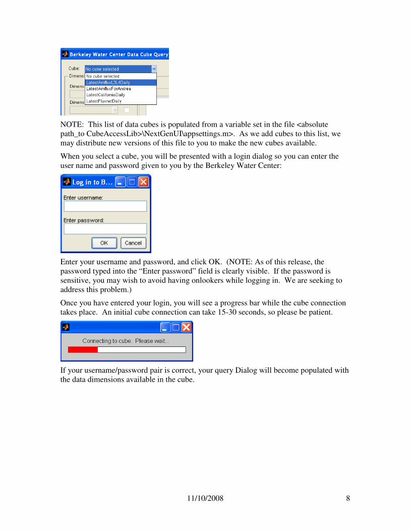
Select a data cube with the drop-down menu at the top of the dialog:

11/10/2008 8

NOTE: This list of data cubes is populated from a variable set in the file <absolute

path_to CubeAccessLib>\NextGenUI\appsettings.m>. As we add cubes to this list, we

may distribute new versions of this file to you to make the new cubes available.

When you select a cube, you will be presented with a login dialog so you can enter the

user name and password given to you by the Berkeley Water Center:

Enter your username and password, and click OK. (NOTE: As of this release, the

password typed into the “Enter password” field is clearly visible. If the password is

sensitive, you may wish to avoid having onlookers while logging in. We are seeking to

address this problem.)

Once you have entered your login, you will see a progress bar while the cube connection

takes place. An initial cube connection can take 15-30 seconds, so please be patient.

If your username/password pair is correct, your query Dialog will become populated with

the data dimensions available in the cube.

11/10/2008 9

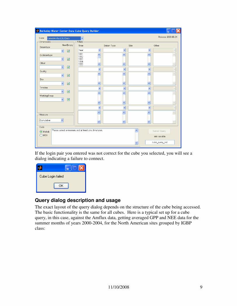
If the login pair you entered was not correct for the cube you selected, you will see a

dialog indicating a failure to connect.

Query dialog description and usage

The exact layout of the query dialog depends on the structure of the cube being accessed.

The basic functionality is the same for all cubes. Here is a typical set up for a cube

query, in this case, against the Amflux data, getting averaged GPP and NEE data for the

summer months of years 2000-2004, for the North American sites grouped by IGBP

class:

11/10/2008 10

To query the cube, you select filter, dimension, and measure criteria with the dialog

controls, and click the Submit Query button to issue the query. The results are placed in

a global structure variable, as described in the Result Data Structure section of this

document.

Dimensions

At least one data dimension must be selected for query, and usually more are desired.

Data returned from the query is inherently multidimensional. The total number of

elements in a returned data set will be the product of the sizes of all dimensions

multiplied together. A single data element from within the returned dataset is specified

by a single location index along each dimension.

A data dimension may be simple such that it is either

selected or not selected (such as datumtype), or may have

numerous resolutions and types of aggregation available.

An example of this is the Timeline dimension, which can

be set to aggregate data by year, year down to the month,

year down to the day, collect all months of the various

year together for seasonality studies, etc.

11/10/2008 11

When you select dimensions, the order of the returned dimensions will be in the top-

down order that they are shown in the query dialog. Thus, in the example figure where

timeline, datumtype, and site are selected, their respective positions in the return array

would be 1, 2, and 3.

The Non-Empty checkbox is offered to cut down on blank data delivery from sparse

cubes. This can be desirable in large return sets since even blank data elements (NaN)

take up memory and are communicated over the network. If Non-Empty is checked, any

dimension member that has no associated data will not be included in the return set. For

example, if you were calling for yearly measurement counts of GPP for all sites between

the years of 2000 and 2007, and had checked Non-Empty for the timeline, and there were

no measurements of this value in 2005 at all, the position for 2005 would be omitted from

the results and the timeline axis would show labels of ‘2000’, ‘2001’, ‘2002’, ‘2003’,

‘2004’, ‘2006’, and ‘2007’.

Measure

The Measure is the way raw data measurements from the cube are aggregated together to

form product data elements in the returned dataset. Examples are:

Count: The number of raw measurements that are available to be aggregated through the

permutations of the various axis members.

Average: The mean values of raw measurements aggregated through the permutations of

the various axis members.

Cumulative: The sum of values of raw measurements aggregated through the

permutations of the various axis members.

MinimumValue/MaximumValue: The lowest or highest, respectively, of the aggregated

raw measurements.

Filters

Filters exclude data that have not been specifically selected from being included in the

query results. This is very important for insuring that certain values (for example, data

collection sites not part of a given study) are not aggregated into collective results (such

as by-year cumulative measures for entire classes of sites). Filters can also be important

when querying very fine-scale data, which can be voluminous across the full time and

geographic scales of the cube, and could cause queries to be very slow or even fail due to

memory constraints.

Criteria for filtering are arranged into sets. For example, the set “Years” along the

Timeline dimension contains the individual data years available in the cube, the “SiteID”

set contains the identifies for each data collection site, and so on.

In the Filters section of the Query Dialog, there are 16 control pairs of a drop-down menu

and a list box. The drop-down menu is used to select the filter set, and selecting the set

causes the associated list box to become populated with the individual members of the

filter set. You can then select the members of the filter set from which you desire data.

11/10/2008 12

The filter sets are arranged into four columns according to function. The leftmost column

contains filter sets pertaining to time of measurement. The second column is for type of

data measurement (variable being measured). The third column pertains to geographic

location of measurement (site). The fourth column is for available filter sets that may not

fall into these three categories

For example, you may wish to filter data to access only certain years of interest. In the 1st

filter column, you can select the set “Year” in the drop down menu:

(NOTE: This “Year” set is generally pre-selected automatically on log-in to the cube.

This is to provide a “hint” as to the functioning of the filters, and that the log-in was

successful.)

The “Year” list box will be populated with the data-years available, and you can select

the years you want by clicking the individual years. If you wish to

select a range of filter members, you can hold down the Shift key

while you click the first and then the last item in the box. If you want

to select multiple discontiguous items, you can hold down the Control

(Ctrl) key while selecting items one-by one.

Here the years 2002-2004 plus 2006 have been selected:

As you select filter sets, selected filter sets will become unavailable in other filter drop-

down menus, because a particular filter set can only be used once in a query.

IMPORTANT NOTE ON FILTERING: Filters are use to exclude data other than that

selected. You do not need to use filter sets when you do not wish to exclude anything in

the set. For instance, if you want precipitation data for each day of year 2002, you DO

need to select “Day of Year” as a Timeline dimension, and select Year as a time filter set,

selecting the year 2002 within that set. You should NOT try to select “Day of Year” as a

filter set for Time, and then select all days of the year. (You actually cannot do this

because the number of filter selections is limited to 200 members.) This would be

unnecessary as data are included by default. Only use filters when there are data to be

excluded from the given grouping of filter criteria.

Filter members from hierarchies

Certain filter listboxes containing groups of filters can interact with each other in a

hierarchical manner. For instance, each cube contains data collected at many geographic

sites. In the Ameriflux cube there are 79 sites. Each site has a vegetation type,

designated by IGBP class, such as grassland (GRA), evergreen needle-leaf forest (ENF),

or cropland (CRO). Such a hierarchical arrangement of sites can be diagrammed this

way (this is a small subset of IGBP classes and sites in a real cube, for clarity):

11/10/2008 13

Here, each IGBP class is a “parent” and has a group of SiteIDs as its “children”.

Out of the many sites available, it can be useful to narrow the list of sites available for

filtering to those of certain IGBP classes of interest. This makes selection of sites easier

as you have a smaller list of sites to search through and don’t have to search through sites

of vegetation types that don’t fit in your study.

Hierarchies in filter list boxes are represented by hyphenated

group names. For example, the IGBP to Site hierarchy described

above would be shown in this drop-down menu under the site

filter column this way:

Here the two levels of the IGBP To Site hierarchy can be found

second from the top in the list, IGBP class and SiteID. If you

choose both of these levels in two separate drop-downs in the site column, you will be

able to use the hierarchy to choose sites based on IGBP class. After selecting both of

these levels, the filter boxes will look like this:

IGBP to Site

CRO ENF GRA IGBP Classes

SiteIDs

US-ARb

US-ARc

US-Aud

US-Bkg

US-CaV

US-Dk1

US-FPe

US-Fwf

US-Goo

US-IB2

US-Var

US-Wkg

CA-NS1

CA-NS2

CA-NS3

CA-NS4

CA-NS5

US-Fmf

US-Fuf

US-Ha2

US-Ho1

US-KS1

US-Me1

US-Me2

US-Me3

US-Me4

US-NC2

US-ARM

US-Bo1

US-Bo2

US-IB1

US-Ne1

US-Ne2

US-Ne3

Hierarchy

11/10/2008 14

As you choose the “parent” IGBP classes in the upper list box, their “child” SiteIDs will

appear in the lower box. This example illustrates the same hierarchy that was

diagrammed for IGBP classes CRO, ENF, and GRA above:

If you choose more than one parent in the upper level of the hierarchy, the children of all

the selected parents will be displayed in the listbox for the lower level of the hierarchy.

Once the children of the selected parents are displayed, you can then choose the members

that you wish (in this example, SiteIDs) from which you want to select data.

In general, if you select a child level in a hierarchy without its parent being selected, you

will be offered all of the selections in the child level. There is an exception to this.

Sometimes there are so many selections available that they cannot be reasonably

displayed at once, and you are required to select members

from the parent level before and child selections can be

displayed. When this is so, the child level will be marked

with an asterisk (*) in the filter drop-down menu. For

example, our California cube contains over 3700 sites.

This is far too many to display at once. The filter drop-

down menu for sites looks like this:

Here there are two hierarchies that group those 3700+ sites: HUC to

SiteCode and Watershed to SiteName. Using the example of

Watershed to Sitename, if you select only the grouping “*Watershed

to SiteName-Name”, you will not see site names to select.

11/10/2008 15

But if you also select “Watershed to SiteName-Watershed”, and select watersheds in that

list, you will have sites within the selected watershed(s) to choose from:

Result Variable Name

Beneath the Submit Query button is a text box where you can specify the name of a

global variable that will receive the result data structure. It defaults to cube_query_out.

If you are calling for several datasets, you can assign them to different names. To make

the variable available from the command line, issue the command:

global variableName

If you wish your analytical scripts or functions to access it, add the global command to

the analysis code before using the variable.

Code Text Box

As you fill out selections in the query construction dialog, a code line for the

QueryCube() function (described below) is constructed to match the chosen criteria. You

may copy this code (select text with the mouse, Ctrl-C) and paste it into analytical code

of your own. Observing changes in this code while making selections can also be

instructional on how to construct the parameters for this function given the construction

of the particular cube you are using according to your needs.

Note that the username and password for the cube are not embedded into this code, only

variable names for them. You will need to set them before calling QueryCube(), like so:

username = ‘myuser’;

password = ‘mypassword’;

Triggering custom analytical code

If you prefer to use the GUI query builder interface rather than the QueryCube() function,

you may wish to execute your own analytical or data display code once data has been

fetched. There is a hook in the GUI that allows your custom code to be called when you

click the Submit Query button once the query has completed.

To use this hook, place a file named doAnalyses.m in the cube folder that is your

working directory. In that file, create a function:

function doAnalyses(cube_query_out)

11/10/2008 16

where cube_query_out is the query result structure (as described in the previous section)

that will be passed to your code. Remember to test cube_query_out.sucess for true before

operating on the returned data.

You may also choose to place this function file in another folder than your working

folder, but in that case you will need to add that folder to your Matlab path ABOVE the

rest of the cube interface folders. This is to make sure that your customized doAnalyses()

function will be called preferentially over the empty stub in the interface code body.

Using the QueryCube() Function Interface

QueryCube is the code-level interface for cube access without the use of the GUI.

result =

QueryCube(baseurl,dbname,cubename,username,password,measure

,dimnames,dimensions,non_emptys,filters)

Here, result is the query result data structure described previously in this document. It

should be noted that several important supplied parameters (measure, dimensions, and

filters) are strings or cell arrays of strings in the MDX member description format. As

there are several cubes accessible with this interface, and since cubes change in their

construction with fair frequency, it is out of the scope of this document to list the various

member names. Again, it is instructional to the user to use the GUI and observe the

changes in the Matlab code window in response to various selected criteria

Here are the input parameters described in detail and example:

baseurl

A single string containing the base URL of the web server. This string is present in the

file appsettings.m as BASE_URL. At the time of this writing, that base URL is:

'http://bwc.berkeley.edu/mdxconnect/Default.aspx?db='

dbname

A single string containing the name of the SSAS database containing the cube to be

queried. This string is present in the file appsettings.m as DB_NAME.

cubename

A single string containing the name of the cube to be queried. This string is present in

the file appsettings.m as CUBE_NAME.

username

A single string containing the Windows user name used to access the cube.

password

A single string containing the Windows password used to access the cube.

measure

11/10/2008 17

A single string with the MDX member designation of the data measure being queried.

Examples: for the count, '[Measures].[Count]', for the average, '[Measures].[Average]'.

dimnames

A 1-dimensional cell array of strings containing the names of the dimensions called for in

the query. This is actually simply repeated back in the return structure member

results.dim_names, and not included in the query sent to the server. It is used here to

provide consistency with the output of the GUI, which provides the names of the selected

dimensions because otherwise analytical code could not know what the user has selected.

Example: calling for three dimensions, Timeline, Datumtype, and Site, the cell array

would be coded as {'Timeline' 'Datumtype' 'Site'}

dimensions

A 1-dimensional cell array of strings containing the hierarchy designations for each

dimension desired in the query results. Example: calling for three dimensions, Timeline

(by year), Datumtype, and Site (by SiteID), the cell array would be coded for as {'[Timeline].[Year].[Year]' '[Datumtype].[Datumtype].[Datumtype]'

'[Site].[IGBP To Site].[SiteID]'}

non_emptys

A 1-dimensional numeric array of logical values (1-true or 0-false), one for each

dimension called for in the order that they were described. True means that the

dimension is queried as non-empty (no dimension position will be returned where the

entire dimension has no data values), false means that an empty dimension position will

be returned filled with NaN’s. Example (matching previous dimension): Continuous

timeline (regardless of empties), empty datumtypes and siteids not returned would be

coded as [0 1 1]

filters

A one dimensional cell array of one-dimensional cell arrays, one inner array for each set

of filters (equivalent to one of the filter lists in the GUI) called for. Example: filtering

down to the years 2000-2003, datumtype GPP, no exdatumtype or offset, and only sites

of IGBP types DBF and ENF, might be coded as:

{{'[Timeline].[Year].[Year].[2000]' '[Timeline].[Year].[Year].[2001]'

'[Timeline].[Year].[Year].[2002]' '[Timeline].[Year].[Year].[2003]'}

{'[Datumtype].[Datumtype].[GPP]'} {'[Exdatumtype].[Exdatumtype].&[1]'}

{'[Offset].[Offset].&[1]' } {'[Site].[IGBP To Site].[IGBPClass].&[DBF]'

'[Site].[IGBP To Site].[IGBPClass].&[ENF]'}}

Examples of Cube Queries and Analyses

Example 1: 2004 Daily Temperature at Boreal Forest sites outside Canada

Using the Fluxnet Daily cube, here we are asking for daily average temperatures from

any sites covered by the boreal working group, but only for sites outside of Canada. The

object is to make a scatter plot with the day of year on the X axis, and the temperature on

11/10/2008 18

the Y axis. There will be one data point per site/day, and a different symbol for each site.

Colors for the symbols are selected by country.

Setting up the query

The query window, when set up for this inquiry, will look like this:

We will go over the query criteria point-by-point.

Dimensions

The dimensions are time (as day of year) and site. In the

product graph, the time dimension will be displayed along the

X axis, the site dimension expressed as symbol, and the data

values themselves arranged along the Y axis.

Thus, two dimensions are called for:

Timeline as Day of Year

Site as SiteName.

Notes:

11/10/2008 19

• The TimeLine dimension has the Non-Empty checkbox set off. This way if there

happens to be a day of year with no data, that day will still be represented on the

return axis.

• Since only one datum type, air temperature (Ta), is being called for, we have no

need to specify the datum type dimension. The filter we will set will insure that

only Ta values will be included in the returned data set.

Measure

As we are looking for average daily temperatures, we will use the Average measure.

Filters

Time

We only want data for 2004. In the Time column of the filters section, we will select the

Year filter group in a filter drop-down menu, and select the year 2004 from the associated

list box.

Datum Type

We only want one datum type, the air temperature (Ta). In the Datum

Type column of the filters section, we will select the Datumtype filter

group in a filter drop-down menu, and select the year 2004 from the

associated list box.

Site

There are two criteria by which we will filter sites: We want only sites within the boreal

working group, and only sites outside of Canada.

In the Site column of the filters section, we will select the

WorkingGroup filter group in a filter drop-down menu and select

Boreal Working Group from the associated list box. In the next set

of controls in the Datum Type column, we will select the Country

filter group in a filter drop-down menu. We will then select all

countries (there are many ways to do this quickly—try holding down

the Ctrl key and press A for “select all”), then scroll to see Canada,

hold down the Ctrl key and click Canada to deselect Canada from

the list. This will cause data from Canadian sites to be filtered out.

11/10/2008 20

After setting all of these criteria, we press the “Submit Query” button. In the Matlab

window we see

Start Reading cube ....

Elapsed time is 0.002854 seconds.

query submitted

Elapsed time is 0.467295 seconds.

reply received

Elapsed time is 0.480856 seconds.

tokens split

Elapsed time is 0.745432 seconds.

data deserialized

End Reading cube ...

This tells us that the query was successful.

Results

To examine the results of the query, we first gain access to the result structure by entering

at the command line:

>> global cube_query_out

We can look at the names of the dimensions of the returned data with

>> cube_query_out.dim_names

ans =

'Site' 'Timeline'

So the first dimension (column) is the site, the second (row) is timeline. To see how

many elements there are in the axes, we can use:

>> cube_query_out.dim_sizes

ans =

11 366

This shows that we have 11 sites, and 366 days in the leap year 2004.

Let’s view the site names on axis 1 by iterating through the cell array

cube_query_out.axes{1} with the code:

for i=1:cube_query_out.dim_sizes(1)

disp(cube_query_out.axes{1}{i});

end

Finland - Hyytiala

Finland - Kaamanen wetland

Finland - Siikaneva fen

Finland - Sodankyla

Russia - Fedorovskoje-drained spruce stand

Sweden - Degero

Sweden - Skyttorp

11/10/2008 21

USA - AK - Atqasuk

USA - ME - Howland Forest (main tower)

USA - ME - Howland Forest (west tower)

USA - MI - Sylvania Wilderness Area

The actual air temperature data is in the array cube_query_out.data. If we wanted the

temperature for the Finland sites (columns 1-4) for the 30th

of January (the 30th

day of the

year--row 30), we could view them with:

>> cube_query_out.data(1:4,30)

ans =

-7.8342

-13.0844

NaN

-11.4312

This tells us (aside from our Finland sites being cold in January) that there is no data for

Siikaneva fen.

Plotting these data

Here is an example of a script to plot the result data as a time-wise scatter plot.

% make sure we have access to our return data in the global

% data space

global cube_query_out;

% create the figure window with axes

fh = figure();

ah = axes();

% These will be the symbols we use for the various sites

symbols = '+ox*sd^Vph.';

% There's only 366 days, so set limits on the X axis

xlim([1 366]);

% iterate through the sites on the first dimension, choose colors and

% symbols, and plot each site's data series

hold on;

for i=1:cube_query_out.dim_sizes(1)

% choose the color for the country

% we will make an unknown country magenta

color = 'm';

if strfind(cube_query_out.axes{1}{i},'Finland') == 1

color = 'g';

end

if strfind(cube_query_out.axes{1}{i},'Russia') == 1

color = 'r';

end

if strfind(cube_query_out.axes{1}{i},'Sweden') == 1

color = 'k';

end

if strfind(cube_query_out.axes{1}{i},'USA') == 1

color = 'b';

end

% set up the color/symbol as the linespec

linespec = [symbols(i) color];

% plot the site temperatures, day numbers on the X axis, temperature

% data on the Y axis

plot(1:cube_query_out.dim_sizes(2),cube_query_out.data(i,:),linespec);

end

% Set up a legend using the Sites dimension axis

11/10/2008 22

legend(cube_query_out.axes{1},'Location','SouthOutside');

% label our graph

xlabel('Day of Year');

ylabel('Temperature [C]');

title('2004 Daily Temperature at Boreal Forest Sites Outside Canada');

hold off;

The resulting plot looks like this:

Example 2: Availability of Data for Productivity Study

Using the AmeriFlux database, we are planning a study on the relationship between gross

ecosystem production (GPP) and net ecosystem exchange (NEE) in evergreen forests in

North America. We wish to know which evergreen forest sites and which years have the

best coverage of these measurements.

Setting up the query

The query window, when set up for this inquiry, will look like this:

11/10/2008 23

11/10/2008 24

Dimensions

Our interest is in (1) the two datum types GPP and NEE, as

measured at (2) various sites, in the (3) various years of

data available in the data cube. Thus, we have a need for

three dimensions in our results:

Datumtype

Site as SiteID

Timeline as Year

Notes:

• This time the Non-Empty checkbox for The

TimeLine dimension has been set on. We are not

interested in years with no data, and have no need

for years to be contiguous in the result dataset.

• Unlike the previous example, we have more than one datum type to count. We

need to have the datum type distributed along its own dimension so that we can

separate the counts for these two variables.

Measure

We are counting numbers of measurements made during various site years, rather than

being interested in the measurement values themselves. This is what the Count measure

does.

Filters

Since we are looking across the entire time-scope of the database by year to search for

likely site-years for a study, we have no need to set any filters on

Time.

Of the many data variables available, we are only interested in two,

GPP and NEE. In the Datum Type filter column we will select

Datumtype as a filter group, and holding down the Ctrl key (to

select multiple individual items) select GPP and NEE in the

listbox.

We are only interested in North American sites, and the North

American countries covered by the AmeriFlux database are

Canada and the US. Under the Site filters column, we will select

the Country group, and choose Canada and USA by holding down

the Shift key and dragging the mouse over the two countries in the

list box.

11/10/2008 25

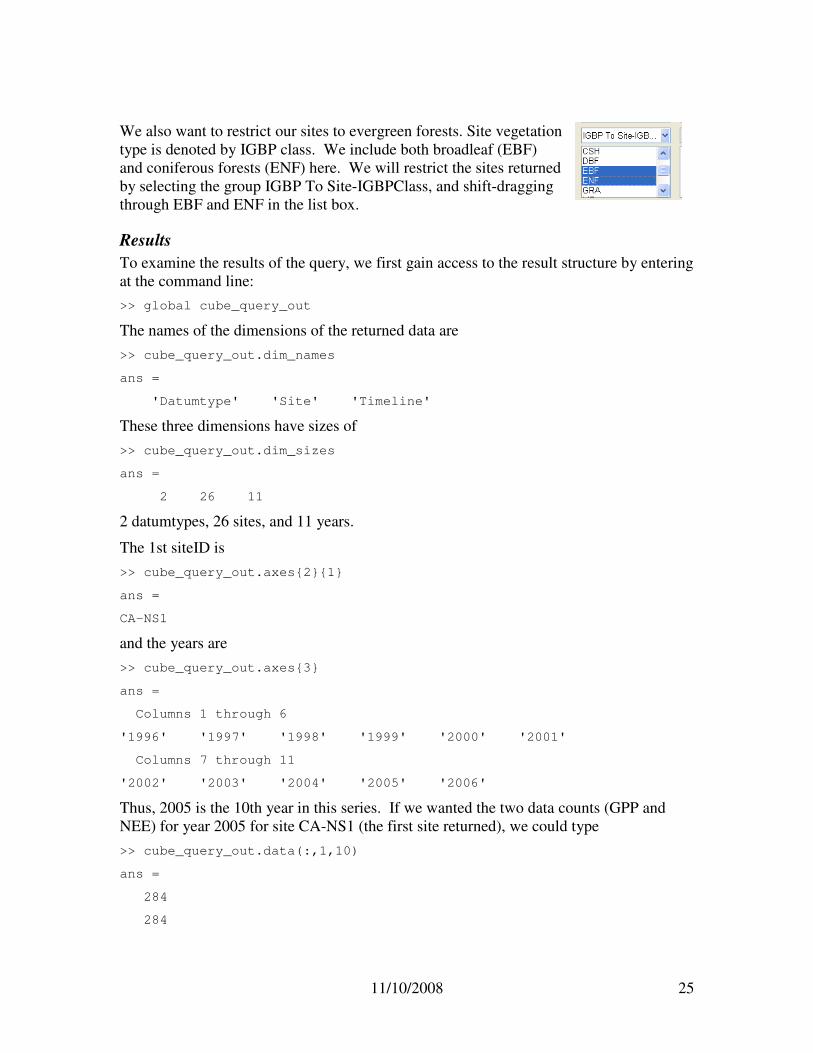
We also want to restrict our sites to evergreen forests. Site vegetation

type is denoted by IGBP class. We include both broadleaf (EBF)

and coniferous forests (ENF) here. We will restrict the sites returned

by selecting the group IGBP To Site-IGBPClass, and shift-dragging

through EBF and ENF in the list box.

Results

To examine the results of the query, we first gain access to the result structure by entering

at the command line:

>> global cube_query_out

The names of the dimensions of the returned data are

>> cube_query_out.dim_names

ans =

'Datumtype' 'Site' 'Timeline'

These three dimensions have sizes of

>> cube_query_out.dim_sizes

ans =

2 26 11

2 datumtypes, 26 sites, and 11 years.

The 1st siteID is

>> cube_query_out.axes{2}{1}

ans =

CA-NS1

and the years are

>> cube_query_out.axes{3}

ans =

Columns 1 through 6

'1996' '1997' '1998' '1999' '2000' '2001'

Columns 7 through 11

'2002' '2003' '2004' '2005' '2006'

Thus, 2005 is the 10th year in this series. If we wanted the two data counts (GPP and

NEE) for year 2005 for site CA-NS1 (the first site returned), we could type

>> cube_query_out.data(:,1,10)

ans =

284

284

11/10/2008 26

So there are 284 data items for each of the variables GPP and NEE from the site CA-NS1

in year 2005.

Tabulating these data

The following script will print a table with the two variables for each year in the columns,

one site per row.

% make sure we have access to our return data in the global

% data space

global cube_query_out;

% set up variables for the dimension counts for easier reading

num_variables = cube_query_out.dim_sizes(1);

num_sites = cube_query_out.dim_sizes(2);

num_years = cube_query_out.dim_sizes(3);

% create a partial header line with the variable names by iterating

% through the variables axis

varhead = '';

for i=1:num_variables

% concatinate the variable names with 2 spaces between

varhead = [varhead cube_query_out.axes{1}{i} ' '];

end

% Create two header lines by iterating through the years

header1 = 'SiteID ';

header2 = ' ';

for i=1:num_years

% concatenate the years together with six spaces in between

header1 = [header1 cube_query_out.axes{3}{i} ' '];

% concatenate the variable names together for the second line

header2 = [header2 varhead];

end

% a title to start

disp(' ');

disp('GPP and NEE data counts for AmeriFlux evergreen forest sites');

disp(' ');

% print the 2 header lines

disp(header1);

disp(header2);

% Build and print the data lines iterating through each site

for site=1:num_sites

% build the data line for this site

% start the line with the site name, spaces following

line = [cube_query_out.axes{2}{site} ' '];

% iterate through the years

for year=1:num_years

% for each year, iterate through the variables

for var=1:num_variables

% concatinate the data value for this year/variable to the

% data line

if isnan(cube_query_out.data(var,site,year))

% if the value is empty, make it blank instead of printing

% 'NaN', for clarity

line = [line ' '];

else

% otherwise there is a real value, add it to the data line

line = [line sprintf('%d ',...

cube_query_out.data(var,site,year))];

end

end

end

11/10/2008 27

% print out the data line for the site

disp(line);

end

The script produces the following table:

GPP and NEE data counts for AmeriFlux evergreen forest sites

SiteID 1996 1997 1998 1999 2000 2001 2002 2003 2004 2005 2006

GPP NEE GPP NEE GPP NEE GPP NEE GPP NEE GPP NEE GPP NEE GPP NEE GPP NEE GPP NEE GPP NEE

CA-NS1 175 175 360 360 366 366 284 284

CA-NS2 173 173 352 352 306 306 333 333 141 141

CA-NS3 173 173 365 365 365 365 366 366 281 281

CA-NS4 365 365 366 366

CA-NS5 143 143 343 343 281 281 365 365 281 281

US-Fmf 170 170 256 256

US-Fuf 130 130 257 257

US-Ha2 208 208

US-Ho1 366 366 365 365 365 365 365 365 366 366 365 365 365 365 365 365 366 366

US-KS1 309 309

US-Me1 214 214 149 149

US-Me2 305 305 350 350 365 365

US-Me3 366 366 365 365

US-Me4 283 283 323 323 240 240 360 360 363 363

US-NC2 361 361 365 365

US-NR1 365 365 366 366 365 365 365 365

US-SP1 192 192 246 365 365 365

US-SP2 127 127 243 333 366 366 365 365 365 365 365 365 366 366

US-SP3 359 359 152 152 365 365 365 365 359 359 366 366

US-SP4 182 182

US-Wi0 261 261

US-Wi2 239 239

US-Wi4 231 231 215 215 259 259 191 191

US-Wi5 260 260

US-Wi9 243 243 116 116

US-Wrc 241 241 365 365 366 366 365 365 365 365 366 366 114 114 365 365