TECHNICAL REVIEWNo. 1 – 2010

HEADQUARTERS: Brüel & Kjær Sound & Vibration Measurement A/S DK-2850 Nærum Denmark · Telephone: +45 7741 2000 · Fax: +45 4580 1405 www.bksv.com · info@bksv.com

Local representatives and service organisations worldwide

BV00

62–

11IS

SN00

07–

2621

ËBV-0062---'Î

Time Selective Response MethodIn situ Measurement of Absorption Coefficient

Transverse Motion in Accelerometer Calibration

Previously issued numbers ofBrüel & Kjær Technical Review1 – 2009 Use of Volume Velocity Sound Sources in the Measurement of Acoustic

Frequency Response FunctionsTurnkey Free-field Reciprocity System for Primary Microphone Calibration

1 – 2008 ISO 16063–11: Primary Vibration Calibration by Laser Interferometry: Evaluation of Sine Approximation Realised by FFTInfrasound Calibration of Measurement MicrophonesImproved Temperature Specifications for Transducers with Built-in Electronics

1 – 2007 Measurement of Normal Incidence Transmission Loss and Other Acoustical Properties of Materials Placed in a Standing Wave Tube

1 – 2006 Dyn-X Technology: 160 dB in One Input RangeOrder Tracking in Vibro-acoustic Measurements: A Novel ApproachEliminating the Tacho ProbeComparison of Acoustic Holography Methods for Surface Velocity Determination on a Vibrating Panel

1 – 2005 Acoustical Solutions in the Design of a Measurement Microphone for Surface MountingCombined NAH and Beamforming Using the Same ArrayPatch Near-field Acoustical Holography Using a New Statistically Optimal Method

1 – 2004 Beamforming1 – 2002 A New Design Principle for Triaxial Piezoelectric Accelerometers

Use of FE Models in the Optimisation of Accelerometer DesignsSystem for Measurement of Microphone Distortion and Linearity from Medium to Very High Levels

1 – 2001 The Influence of Environmental Conditions on the Pressure Sensitivity of Measurement MicrophonesReduction of Heat Conduction Error in Microphone Pressure Reciprocity CalibrationFrequency Response for Measurement Microphones – a Question of ConfidenceMeasurement of Microphone Random-incidence and Pressure-field Responses and Determination of their Uncertainties

1 – 2000 Non-stationary STSF1 – 1999 Characteristics of the Vold-Kalman Order Tracking Filter1 – 1998 Danish Primary Laboratory of Acoustics (DPLA) as Part of the National

Metrology OrganisationPressure Reciprocity Calibration – Instrumentation, Results and UncertaintyMP.EXE, a Calculation Program for Pressure Reciprocity Calibration of Microphones

(Continued on cover page 3)

1 – 1997 A New Design Principle for Triaxial Piezoelectric AccelerometersA Simple QC Test for Knock SensorsTorsional Operational Deflection Shapes (TODS) Measurements

2 – 1996 Non-stationary Signal Analysis using Wavelet Transform, Short-time Fourier Transform and Wigner-Ville Distribution

1 – 1996 Calibration Uncertainties & Distortion of Microphones.Wide Band Intensity Probe. Accelerometer Mounted Resonance Test

2 – 1995 Order Tracking Analysis1 – 1995 Use of Spatial Transformation of Sound Fields (STSF) Techniques in the

Automative Industry2 – 1994 The use of Impulse Response Function for Modal Parameter Estimation

Complex Modulus and Damping Measurements using Resonant and Non-resonant Methods (Damping Part II)

1 – 1994 Digital Filter Techniques vs. FFT Techniques for Damping Measurements (Damping Part I)

2 – 1990 Optical Filters and their Use with the Type 1302 & Type 1306 Photoacoustic Gas Monitors

1 – 1990 The Brüel & Kjær Photoacoustic Transducer System and its Physical Properties

2 – 1989 STSF – Practical Instrumentation and ApplicationDigital Filter Analysis: Real-time and Non Real-time Performance

1 – 1989 STSF – A Unique Technique for Scan Based Near-Field Acoustic Holography Without Restrictions on Coherence

2 – 1988 Quantifying Draught Risk1 – 1988 Using Experimental Modal Analysis to Simulate Structural Dynamic

ModificationsUse of Operational Deflection Shapes for Noise Control of Discrete Tones

Special technical literatureBrüel & Kjær publishes a variety of technical literature which can be obtained from your local Brüel & Kjær representative.

The following literature is presently available:

• Catalogues (several languages)• Product Data Sheets (English, German, French,)

Furthermore, back copies of the Technical Review can be supplied as listed above. Older issues may be obtained provided they are still in stock.

Previously issued numbers ofBrüel & Kjær Technical Review(Continued from cover page 2)

TechnicalReviewNo. 1 – 2010

Contents

Time Selective Response Measurements – Good Practices and Uncertainty........ 1Erling Sandermann Olsen and Rémi Guastavino

Measurement of Absorption Coefficient, Radiated and Absorbed Intensity on the Panels of a Vehicle Cabin using a Dual Layer Array with Integrated Position Measurement........................................................................................................ 16J. Hald, J. Mørkholt and S. Gade

ISO 16063–11: Uncertainties in Primary Vibration Calibration by Laser Interferometry – Reference Planes and Transverse Motion ................................ 28Torben Licht and Sven Erik Salbøl

TRADEMARKS

PULSE is a trademark of Brüel & Kjær Sound & Vibration Measurement A/S

Copyright © 2010, Brüel & Kjær Sound & Vibration Measurement A/SAll rights reserved. No part of this publication may be reproduced or distributed in any form, or by any means, without prior written permission of the publishers. For details, contact: Brüel & Kjær Sound & Vibration Measurement A/S, DK-2850 Nærum, Denmark.

Editor: Harry K. Zaveri

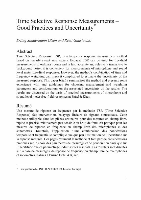
Time Selective Response Measurements – Good Practices and Uncertainty*

Erling Sandermann Olsen and Rémi Guastavino

AbstractTime Selective Response, TSR, is a frequency response measurement methodbased on linearly swept sine signals. Because TSR can be used for free-fieldmeasurements in ordinary rooms and is fast, accurate and relatively insensitive tobackground noise, it is convenient for measurements of microphone and soundlevel meter free-field responses. However, the method’s combination of time andfrequency weighting can make it complicated to estimate the uncertainty of themeasured response. This paper briefly summarizes the method and presents someexperience with and guidelines for choosing measurement and weightingparameters and considerations on the associated uncertainty on the results. Theresults are discussed on the basis of practical measurements of microphone andsound level meter free-field responses at Brüel & Kjær.

RésuméUne mesure de réponse en fréquence par la méthode TSR (Time SelectiveResponse) fait intervenir un balayage linéaire de signaux sinusoïdaux. Cetteméthode utilisable dans les pièces ordinaires pour des mesures en champ libre,rapide et précise, relativement peu sensible au bruit de fond, est pratique pour lesmesures de réponse en fréquence en champ libre des microphones et dessonomètres. Toutefois, l’application d’une combinaison des pondérationstemporelle et fréquentielle complique quelque peu l’estimation de l’incertitude surla réponse mesurée. Ces pages résument la méthode et font part de considérationspratiques sur le choix des paramètres de mesurage et de pondération ainsi que surl’incertitude que ce paramétrage induit sur les résultats. Ces résultats sont discutéssur la base de mesurages de réponse de fréquence en champ libre de microphoneset sonomètres réalisés à l’usine Brüel & Kjaer.

* First published at INTER-NOISE 2010, Lisbon, Portugal

1

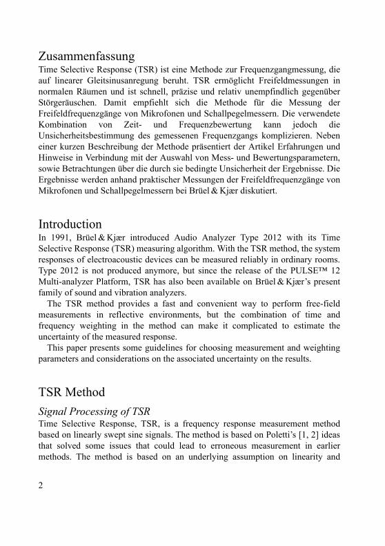
ZusammenfassungTime Selective Response (TSR) ist eine Methode zur Frequenzgangmessung, dieauf linearer Gleitsinusanregung beruht. TSR ermöglicht Freifeldmessungen innormalen Räumen und ist schnell, präzise und relativ unempfindlich gegenüberStörgeräuschen. Damit empfiehlt sich die Methode für die Messung derFreifeldfrequenzgänge von Mikrofonen und Schallpegelmessern. Die verwendeteKombination von Zeit- und Frequenzbewertung kann jedoch dieUnsicherheitsbestimmung des gemessenen Frequenzgangs komplizieren. Nebeneiner kurzen Beschreibung der Methode präsentiert der Artikel Erfahrungen undHinweise in Verbindung mit der Auswahl von Mess- und Bewertungsparametern,sowie Betrachtungen über die durch sie bedingte Unsicherheit der Ergebnisse. DieErgebnisse werden anhand praktischer Messungen der Freifeldfrequenzgänge vonMikrofonen und Schallpegelmessern bei Brüel & Kjær diskutiert.

Introduction In 1991, Brüel & Kjær introduced Audio Analyzer Type 2012 with its TimeSelective Response (TSR) measuring algorithm. With the TSR method, the systemresponses of electroacoustic devices can be measured reliably in ordinary rooms.Type 2012 is not produced anymore, but since the release of the PULSE™ 12Multi-analyzer Platform, TSR has also been available on Brüel & Kjær’s presentfamily of sound and vibration analyzers.

The TSR method provides a fast and convenient way to perform free-fieldmeasurements in reflective environments, but the combination of time andfrequency weighting in the method can make it complicated to estimate theuncertainty of the measured response.

This paper presents some guidelines for choosing measurement and weightingparameters and considerations on the associated uncertainty on the results.

TSR Method

Signal Processing of TSRTime Selective Response, TSR, is a frequency response measurement methodbased on linearly swept sine signals. The method is based on Poletti’s [1, 2] ideasthat solved some issues that could lead to erroneous measurement in earliermethods. The method is based on an underlying assumption on linearity and

2

invariance of the object response. The impulse response of the system isdetermined by combining the inverted excitation signal with the response signal.Reflections can be excluded from the measurement by selecting the desired part ofthe impulse response by weighting with a time window.

The excitation signal in TSR is a complex, linear sweep:

(1)

The resulting output signal is:

(2)

where h(t) is the impulse response of the object response, the transfer function ofthe complete measurement setup and the surrounding room. In the analysis, theoutput signal is combined with the inverse sweep:

(3)

Inserting ξ = kt, this has the form:

(4)

s t ejkt

2

=

y t h t s t h e jk t – 2 d

–

= =

u t ej– kt

2

y t

ej– kt

2

h e jk t – 2 d

–

ej– kt

2

h ejk t

2 22t–+

d

–

h e jk2

ej2kt– d

–

=

=

=

=

u h e jk2

ej2– d

–

=

3

The integral is recognised as the Fourier transform of the product of the systemimpulse response and the linear sweep, . Hence, using the convolutiontheorem:

(5)

From this it is seen that h(t) can be calculated for any point in time from thecomplete response. In particular, the time range including the direct sound fromthe measurement object can be selected for further calculation. The frequencyresponse function can then be calculated by Fourier transform of h(t):

H(f) = F{h(t)} (6)

Conceptually, TSR can be understood as a combination of the swept sine signaland a tracking filter that follows the signal with a delay so that only thefrequencies arriving at a certain delay are included in the measurement. Thetracking filter is equivalent to the weighting function that defines the selected timerange (Fig. 1).

The TSR algorithm effectively works as a zoom FFT around the centre of theswept frequency range, i.e., the impulse response that is determined is frequencyshifted to the centre frequency of the sweep. This property means that the sweepdoes not need to cover the full frequency range of the target transfer function.

The TSR method requires measurement of the complex response function. If themeasured frequency range is limited so that negative frequencies are not includedin the full sweep, the complete function can be calculated from a single sinesweep, but if the sweep includes zero or negative frequencies, a cosine andsubsequently a sine sweep must be made in order to obtain the complex function.

Windows in TSR In addition to the time window that is (or can be) deliberately applied to the timeresponse in a TSR measurement, there are two window functions inherentlyapplied to the signal.

h t e jkt2

h t ej– kt

2

F1–

u

ej– kt

2

u e j2t d

–

=

=

4

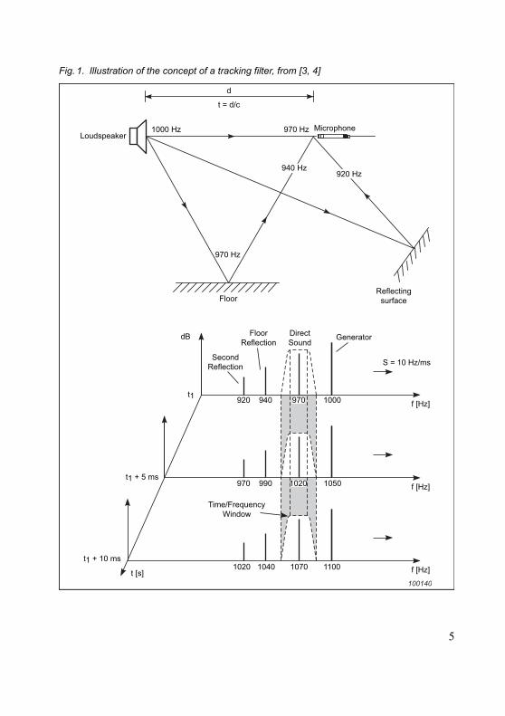
Fig. 1. Illustration of the concept of a tracking filter, from [3, 4]

1000 Hz 970 Hz

970 Hz

Reflectingsurface

d

t = d/c

Floor

940 Hz

LoudspeakerMicrophone

920 Hz

dB

t1 920 940 1000

970 990 1050

1020 1040 1070 1100

S = 10 Hz/ms

f [Hz]

f [Hz]

f [Hz]

Time/FrequencyWindow

t1 + 5 ms

t1 + 10 ms

SecondReflection

GeneratorDirectSound

FloorReflection

t [s]

970

1020

100140

5

The first window inherent to the method is due to the limitation of the frequencysweep to the specified range. This is equivalent to applying a window function toan infinitely long frequency sweep:

(7)

The frequency spectrum of the finite sweep is determined by this weightingfunction.

The combination with the inverse (unweighted) sweep does not by itself distortthe resulting impulse response.

The second window inherent to the method is due to the limitation of theanalysis to a certain time range, and this is also effectively an application of awindow to the impulse response, the time range mentioned above:

(8)

The second window defines the time range that is included in the final Fouriertransform so as to obtain the frequency response. Subsequent application of anarrower time window in order to exclude reflections is effectively the same asnarrowing the time range, except that the time steps and frequency steps in theanalysis are maintained.

The windows that are applied in Brüel & Kjær’s TSR analyzers are Tukeywindows, i.e., rectangular windows tapered with raised cosine functions. The user-selectable time window is a generalised form where the width of the two taperscan be selected independently.

In order to minimise the influence of the window applied to the sweep, theactual sweep covers a larger frequency range than that specified for the analysis.

The influence of the windows on the final result not only depends on thewindows themselves, but is also a combination of the windows and the response tobe measured. Therefore, it is not possible to predict the exact uncertainty based onthe measurement parameters alone.

s t W1 t e jkt2

=

h t W2 t e j– kt2

u e j2t d

–

=

6

Applications of TSR Since the TSR method provides time selectivity and both the time and frequencyresponses are immediately available, it is convenient for a large range ofapplications.

The method can be used for accurate and fast comparison calibration ofmicrophones and sound level meters and measurement of the influence ofaccessories, etc. Due to the time selectivity, no anechoic chamber is needed for themeasurements.

The method can be used for simple absolute frequency response measurementsof, for example, loudspeakers. A procedure for combining far-field measurementswith the TSR method with traditional near-field measurements for a loudspeaker isdescribed in [5].

Another useful application of the TSR method is to use it as an effective meansfor localising reflections in a measured response. This can be used in optimisingdevices to disturb a sound field as little as possible. In particular this is relevantduring the development of sound level meters, microphone holders, loudspeakerenclosures and similar devices.

Parameter Choice

Sweep LengthAs can be seen from the expressions in “Signal Processing of TSR” on page 2, thesweep rate, and thus the sweep length, only influences the integration time, not theresolution of the measured impulse response. This means that the sweep lengthonly influences the signal-to-noise ratio of the measurement. Some investigationshould be done with the signal-to-noise ratio. If lowering the signal level by 10 dBsignificantly changes the measured response, the signal-to-noise ratio should beimproved. If the noise itself cannot be reduced or the signal level increased, thereare two ways to improve the signal-to-noise ratio in the TSR method. Either thesweep length or the number of averages must be increased. The sweep length doesnot have any other influence on the measurement result, provided that theunderlying overall assumption on linearity and invariance of the system isfulfilled.

Frequency Range The choice of frequency range in the measurement has only minor influence onthe measurement. This is due to the fact that TSR effectively works as a zoom FFT

7

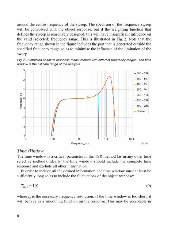
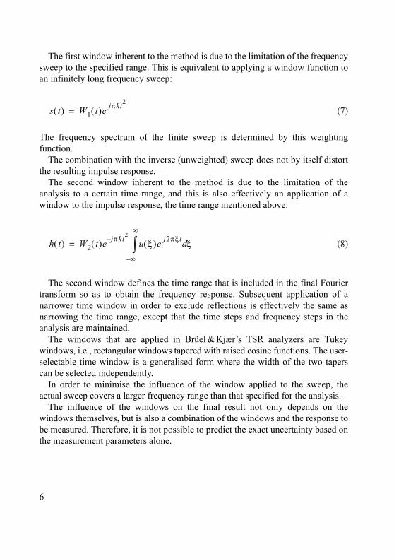
around the centre frequency of the sweep. The spectrum of the frequency sweepwill be convolved with the object response, but if the weighting function thatdefines the sweep is reasonably designed, this will have insignificant influence onthe valid (selected) frequency range. This is illustrated in Fig. 2. Note that thefrequency range shown in the figure includes the part that is generated outside thespecified frequency range so as to minimise the influence of the limitation of thesweep.

Time WindowThe time window is a critical parameter in the TSR method (as in any other timeselective method). Ideally, the time window should include the complete timeresponse and exclude all other information.

In order to include all the desired information, the time window must at least besufficiently long so as to include the fluctuations of the object response:

Tmin = 1/fc (9)

where fc is the necessary frequency resolution. If the time window is too short, itwill behave as a smoothing function on the response. This may be acceptable in

Fig. 2. Simulated absolute response measurement with different frequency ranges. The timewindow is the full time range of the analysis

–4

–3

–2

–1

0

1

2

3

Frequency, Hz

Res

pons

e, d

B

500 – 22k

100 – 5k

100 – 2k

250 – 5k

250 – 10k

250 – 22k

100 – 25k

Correct

10 100 1k 10k 100k100141

8

some cases at high frequencies, for example in relative measurements where theresolution is not required in the measured ratio, but if the object response rolls offat low frequencies, too short a time window may deteriorate a large part of theobject response.

The geometry of the measurement setup should be considered carefully. Simplemeasurement of the size of the measurement object helps in determining theminimum time window, and geometrical consideration can also help in optimisingthe path length difference in the setup.

In a normal building, the open height below room lighting, etc., is typicallyaround 2.5 m. With a measuring distance of 1 m to 2 m, this leaves a differencebetween the direct path and the first reflected path of 1.2 m to 1.7 m,corresponding to a time difference between the direct sound and the first reflectionof 3.5 ms to 4.9 ms. This limits the low-frequency resolution that can be achievedin time selective measurements in normal-sized rooms. If a higher resolution isdesired, a room must be used where the distance to any reflecting objects is larger.This may, however, require more bulky mounting devices that again may lead toless stable mounting and be more susceptible to the movement of air in the room.A time window allowing measurement of a 3.5 ms long time response will besufficient for most applications within microphone and loudspeakermeasurements.

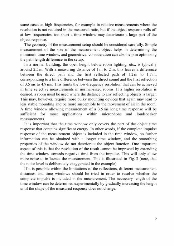
It is important that the time window only covers the part of the object timeresponse that contains significant energy. In other words, if the complete impulseresponse of the measurement object is included in the time window, no furtherinformation can be obtained with a longer time window, and the smoothingproperties of the window do not deteriorate the object function. One importantaspect of this is that the resolution of the result cannot be improved by extendingthe time window towards negative time from the impulse. This will only allowmore noise to influence the measurement. This is illustrated in Fig. 3 (note, thatthe noise level is deliberately exaggerated in the example).

If it is possible within the limitations of the reflections, different measurementdistances and time windows should be tried in order to resolve whether thecomplete impulse is included in the measurement. The necessary length of thetime window can be determined experimentally by gradually increasing the lengthuntil the shape of the measured response does not change.

9

Uncertainty EstimationUncertainty estimation of frequency response measurements made with the TSRmethod is, of course, similar to that of any other frequency response measurementmethod, except for the aspects that are particular to the method. Here, the aspectsrelated to TSR are discussed. Note, that these aspects are to some extent the samefor other time selective methods, because the underlying principle of determiningthe impulse response and selecting a certain part is common to all these methods.

As mentioned and demonstrated, it is not possible to predict the exactuncertainty based on the measurement parameters alone. Some evaluation can bemade on the maximum variation that can be anticipated, but that is likely to lead tooverestimation of the uncertainty. Instead, the evaluation should be based oncontrolled variations or realistic modelling of the actual measurement situation.

In the case of the measurement of a single response, for example, in aloudspeaker measurement, the influence of the windows on the responsecontribute directly to the uncertainty of the measurement. If some knowledge isavailable of the object response, the influence of the parameters can be estimatedby modelling. Alternatively, the measurement can be repeated with variations ofthe parameters. It should, however, be kept in mind that there may be systematicdeviations that are not revealed by the possible parameter variations.

In the case of relative measurements where the response of the measurementobject is compared with the response of a reference, for example, in microphonecomparison calibration or measurement, some of the deviations due to the

Fig. 3. Noise influence. Left: Time window covering the impulse response. Right: time windowextended towards negative time

100 1k 10k–30

–29

–28

–27

–26

–25

–24

–23

100 1k 10k–30

–29

–28

–27

–26

–25

–24

–23

100142

10

windows cancel out because they are present in both measurements. In this casethere are also considerable possibilities of making the measurements underdifferent conditions both in the physical measurement setup and in themeasurement parameters, thereby achieving knowledge on the uncertainty in themeasurements.

In a frequency range where the reference and the object under test have similarand reasonably flat frequency responses, the low-frequency resolution does nothinder an accurate determination of the difference between the two, and theuncertainty on the determined frequency response can be relatively small if care istaken to avoid systematic errors.

ExamplesIn this section, a couple of examples of these measurements are used forillustration of the issues mentioned above. The TSR method is used extensively atBrüel & Kjær for measurements of free-field responses. It is the company’s policyto thoroughly document all electroacoustic devices developed, and the TSRmethod has worked as an efficient and accurate tool for that purpose for severalyears.

Microphone Free-field Response Measurements Free-field response measurements of microphones at Brüel & Kjær are exclusivelymade using the TSR method. Absolute free-field sensitivities are measured bycomparison with reference microphones that are traceable to Danish nationalstandards. Measurements of the influence of accessories such as wind screens,protection grids, etc., and directional characteristics are relative measurementswhere only the stability of the measurement object and the measurement setup isrelevant. However, the measurements are always relative measurements. The free-field measurements with the TSR method are made at frequencies above 500 Hz.Below 500 Hz the free-field response of the microphones can reliably beestablished with other methods that are not the subject of this paper.

In order to ensure high accuracy and reproducibility in the measurements, somepractices have been developed. Although these are not directly related to the TSRmethod, they are mentioned here in order to demonstrate how the TSR method isused.

Many of the measurements are carried out in a measurement room situated in anormal office building. Some factors such as circulating air, for example, due toventilation systems, can disturb these measurements. Small pressure pulses are

11

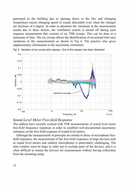
generated in the building due to opening doors or the like and changingtemperature causes changing speed of sound, detectable even when the changesare fractions of a degree. In order to minimise the variations in the measurementresults due to these factors, the ventilation system is turned off during eachresponse measurement that consists of six TSR sweeps. This can be done in aminimum of time. The six sweeps allows the identification of occasional (but rare)variations in the measurements as shown in Fig. 4. The practice also givessupplementary information to the uncertainty estimation.

Sound Level Meter Free-field Response The authors have recently worked with TSR measurements of sound level meterfree-field frequency responses in order to establish well-documented uncertaintyestimates on the free-field response of sound level meters.

Although the measurements in principle are similar to those of microphone free-field responses, the measurement of the free-field responses of large devices suchas sound level meters and outdoor microphones is particularly challenging. Thetime window must be large in order not to exclude parts of the devices, and it isoften difficult to mount the devices for measurement without having reflectionsfrom the mounting setup.

Fig. 4. Variation of six consecutive sweeps. One of the sweeps has been disturbed

–0.2

–0.15

–0.1

–0.05

0

0.05

0.1

0.15

0.2

100Frequency, Hz

Var

iatio

n, d

B

Ignored in average

1k 10k 100k

100143

12

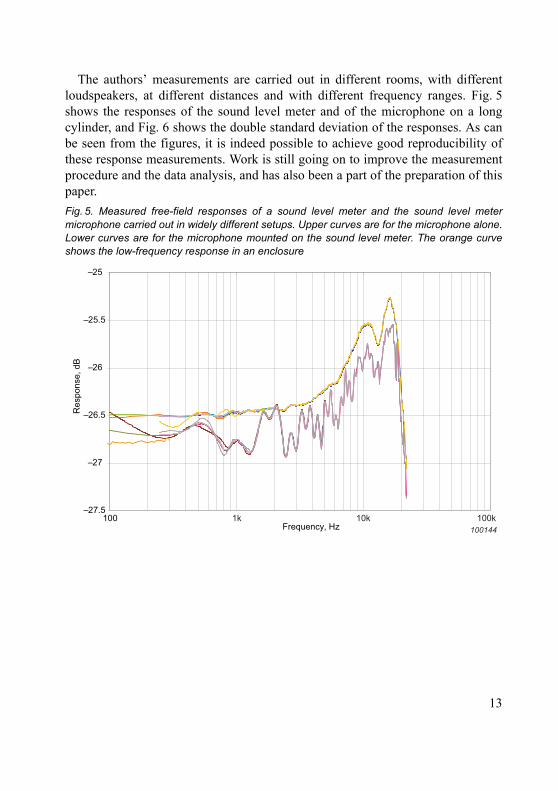
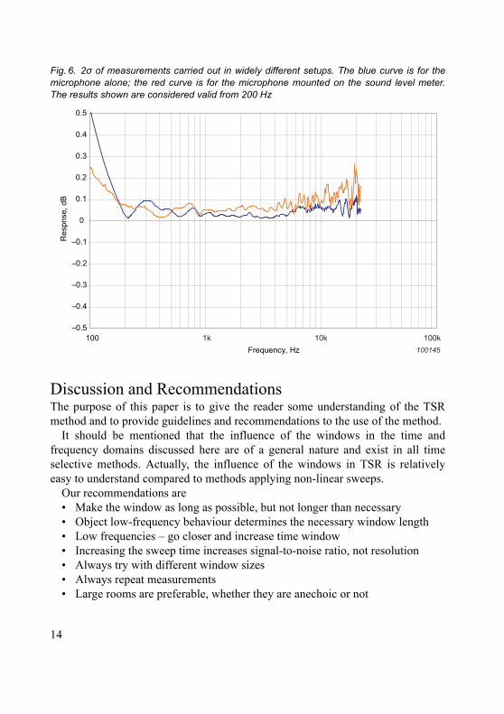
The authors’ measurements are carried out in different rooms, with differentloudspeakers, at different distances and with different frequency ranges. Fig. 5shows the responses of the sound level meter and of the microphone on a longcylinder, and Fig. 6 shows the double standard deviation of the responses. As canbe seen from the figures, it is indeed possible to achieve good reproducibility ofthese response measurements. Work is still going on to improve the measurementprocedure and the data analysis, and has also been a part of the preparation of thispaper.

Fig. 5. Measured free-field responses of a sound level meter and the sound level metermicrophone carried out in widely different setups. Upper curves are for the microphone alone.Lower curves are for the microphone mounted on the sound level meter. The orange curveshows the low-frequency response in an enclosure

–27.5

–27

–26.5

–26

–25.5

–25

Frequency, Hz

Res

pons

e, d

B

100 1k 10k 100k100144

13

Discussion and RecommendationsThe purpose of this paper is to give the reader some understanding of the TSRmethod and to provide guidelines and recommendations to the use of the method.

It should be mentioned that the influence of the windows in the time andfrequency domains discussed here are of a general nature and exist in all timeselective methods. Actually, the influence of the windows in TSR is relativelyeasy to understand compared to methods applying non-linear sweeps.

Our recommendations are • Make the window as long as possible, but not longer than necessary • Object low-frequency behaviour determines the necessary window length • Low frequencies – go closer and increase time window • Increasing the sweep time increases signal-to-noise ratio, not resolution • Always try with different window sizes • Always repeat measurements • Large rooms are preferable, whether they are anechoic or not

Fig. 6. 2σ of measurements carried out in widely different setups. The blue curve is for themicrophone alone; the red curve is for the microphone mounted on the sound level meter.The results shown are considered valid from 200 Hz

–0.5

–0.4

–0.3

–0.2

–0.1

0

0.1

0.2

0.3

0.4

0.5

Frequency, Hz

Res

pnse

, dB

100 1k 10k 100k100145

14

• The air must be stable (easier in ordinary rooms than in anechoic chambers) • Carefully consider the reflections and which to include in the time windowRoutine measurements do not, of course, need to be verified each time.

Summary In this paper, the Time Selective Response method has been summarized and theinfluence of some choices of measurement parameters and their interaction withthe object response have been discussed.

The importance of the right selection of time weighting function has brieflybeen demonstrated. It has also briefly been demonstrated that the actual frequencyrange of the measurement is of small importance.

Some guidelines on how to evaluate the measurement uncertainty due to thetime and frequency limitations in the measurements have also been given.

References [1] Poletti, M. A., “Linearly Swept Frequency Measurements, Time-Delay

Spectrometry, and the Wigner Distribution”, Journal of the AudioEngineering Society, 36 (6), 1988, pp 457 – 468.

[2] Struck, C. J., Biering, C. H., “A New Technique for Fast ResponseMeasurements Using Linear Swept Sine Excitation”, 90th Convention ofthe Audio Engineering Society, New York, USA 1991, preprint 3038.

[3] PULSE™ Time Selective Response (Brüel & Kjær online documentation),Brüel & Kjær, 1995.

[4] Brüel & Kjær, Audio Analyzer Type 2012 Technical Documentation,Brüel & Kjær, BE 1119 – 13, 3–6 to 3–13, 1995 (ca.).

[5] Struck, C. J., Temme, S. F., “Simulated Free Field Measurements”, 93rdConvention of the Audio Engineering Society, New York, USA, 1992,preprint 3397.

15

Measurement of Absorption Coefficient, Radiated and Absorbed Intensity on the Panels of a Vehicle Cabin using a Dual Layer Array with Integrated Position Measurement*

J. Hald, J. Mørkholt and S. Gade

AbstractIn some cases it is important to be able to measure not only the total soundintensity on a panel surface in a vehicle cabin, but also the components of thatintensity due to sound radiation and due to absorption from the incident field. Forexample, these intensity components may be needed for calibration of energy flowmodels of the cabin noise. A robust method based on surface absorptioncoefficient measurement is presented in this paper.

Résumé Dans certaines situations, il est important de pouvoir mesurer non seulementl’intensité acoustique totale sur un panneau de l’habitacle d’un véhicule, maiségalement, du fait de phénomènes de rayonnement sonore et d’absorptioncaractérisant le champ incident, les composantes de cette intensité. Cescomposantes peuvent notamment s’avérer nécessaires pour le calibrage desmodèles de flux d’énergie du bruit généré dans l’habitacle. Une méthode robuste,basée sur la mesure du coefficient d’absorption de la surface, est présentée ici.

ZusammenfassungManchmal ist es wichtig, dass man an einer Innenfläche in der Fahrzeugkabinenicht nur die Gesamtschallintensität misst, sondern außerdem ermitteln kann,welcher Anteil der Intensität auf Schallabstrahlung von der Fläche zurückzuführenist und welcher auf die Absorption von Energie aus dem einfallenden Schallfeld.Diese Intensitätskomponenten werden beispielsweise zur Kalibrierung von

* First published at JSAE Annual Congress 2010, Yokohama, Japan

16

Energieflussmodellen des Kabinengeräuschs benötigt. Dieser Artikel stellt einerobuste Methode vor, die auf der Messung des Absorptionskoeffizienten vonFlächen beruht.

IntroductionConsider the radiation of sound from a small surface segment in a cabinenvironment. Such a surface segment may radiate sound energy because ofexternal forcing, causing the surface to vibrate, and it may absorb energy from anincident sound field because of finite surface acoustic impedance. Whenmeasuring the sound intensity over the surface segment with an intensity probe,the total intensity Itot will be measured. Assuming the radiated field and theincident field to be mutually incoherent, the total intensity is equal to the sum ofthe radiated sound intensity Irad that would exist with no incident field and thesound intensity component Iabs due to absorption from the incident field:

Itot = Irad + Iabs (1)

Considering the intensity in the outward normal direction on the panel surface,the radiated intensity will typically be positive, while the component due toabsorption will typically be negative. So for vibrating panels with an absorptivesurface, the total measured intensity may be small although the radiated intensityis relatively high. Often it is of interest to know not only the total intensity, butalso the components due to radiation and absorption. For example, this kind ofinformation is needed in energy-based modeling that describes the energy flowbetween sub-systems [1].

The method presented here is based on separation of different sound fieldcomponents via the spatial sound field information provided by an array. Theradiated intensity is estimated as the intensity that would exist, if the incident andscattered field components could be removed. So a free-field radiation condition issimulated. The idea is to first separate the incident field component, then useseparately measured information about the scattering properties of the panel tocalculate the scattered field, and finally subtract the incident and scattered fieldsfrom the total sound field. The method needs the panel geometry, which is eitherimported as CAD or measured with a 3D digitizer, and then uses a measured mapof absorption coefficient. The separate measurement of the surface absorptioncoefficient is obtained using loudspeaker excitation.

17

Description of MethodologyThe array measurements considered here are cross-spectral measurements of thefull cross-spectral matrix between all array microphones and, based on that, arepresentation in terms of Principal Components is extracted [2]. As aconsequence, no phase information is available between different array positions,so a separate processing has to be performed for each position. For each PrincipalComponent a separate holography calculation is performed. Since thesecalculations are identical only one will be described. We used a Double LayerArray (DLA), and the processing was performed using Statistically OptimizedNAH (SONAH) [3, 4]. A complex time harmonic representation, with the timevariation e jωt suppressed, will be used.

Extraction of the Incident FieldA basic array processing task is that of extracting the incident sound field from thetotal sound field. However, considering the sound field on a small panel segmentin a cabin, the distinction between the incident field and the radiated field is notobvious, even when we look at the field very near the panel segment. Because ofcoherent vibration components and significant mutual radiation impedancesbetween neighbouring panel segments, some neighbouring segments should beincluded as sources of the radiated field. Fig. 1 illustrates how this distinction canbe made in practice with a DLA. Using SONAH on a DLA measurement, thesound field components (p, u) and (p+, u+) with sources on different sides of thearray plane can be separated, [3, 4]:

(ptotal, utotal) = (p–, u–) + (p+, u+) (2)

The array must then be used in such a way that the pressure p and the velocityvector u represent the field incident on the source area of interest, while theoutward propagating field component (p+, u+) is the sum of the scattered andradiated fields:

(p+, u+) = (psct, usct) + (prad, urad) (3)

Fig. 1a illustrates the case of an isolated source object, where the incident andoutward propagating field components are well-defined. They could bedetermined, for example, based on measurements across two concentric sphericalsurfaces that enclose the test object. Microphones on the two surfaces would be

18

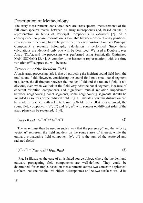
pointing to the centre, but facing in opposite directions. Fig. 1b illustrates the caseof measurement on a panel section in a cabin. In this case, the measurement planewill define the distinction between sources of the incident field and sources of theoutward propagating field. Here a DLA (see Fig. 3) could be used, wheremicrophones are mounted back to back. The distinction will, however, not besharp due to the limited angular resolution of a practical array.

Solution of the Scattering ProblemProvided the incident and radiated fields are mutually incoherent, then Eq. (1) isthe basis for a simple and robust energy based method. The basic assumption isthat we can measure a local absorption coefficient at each point r on the sourcesurface such that the normal components I – and Iabs of the incident and absorbedintensities are related by:

Iabs (r) = (r) I – (r) (4)

In general the ratio Iabs(r)/I –(r) between the two intensities will depend on theform of the incident field. If, however, the coefficient (r) is measured with anincident field that is sufficiently similar to the incident field under operationalconditions, then Eq. (4) can provide good results with the operational field.

The method requires a separate set of DLA measurements with artificial speakerexcitation. Fig. 2 illustrates a setup with a set of incoherently excited speakers tocreate an incident field similar to the field incident under, for example, flightconditions in an aircraft. As mentioned already, the DLA/SONAH measurement

Fig. 1. Separation of inward (incident) and outward propagating field components (p–, u–) and(p+, u+): a) Clearly separated sources. b) Smooth transition between sources

Object

CabinWall

(p–, u–)

(p+, u+) CabinWall

Measurementplane

DLA

Mappingarea

100146

a) b)

19

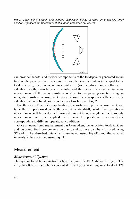
can provide the total and incident components of the loudspeaker generated soundfield on the panel surface. Since in this case the absorbed intensity is equal to thetotal intensity, then in accordance with Eq. (4) the absorption coefficient iscalculated as the ratio between the total and the incident intensities. Accuratemeasurement of the array positions relative to the panel geometry using anintegrated position measurement system allows the absorption coefficients to becalculated at predefined points on the panel surface, see Fig. 2.

For the case of car cabin application, the surface property measurement willtypically be performed with the car at a standstill, while the operationalmeasurement will be performed during driving. Often, a single surface propertymeasurement will be applied with several operational measurements,corresponding to different operational conditions.

Once an operational measurement has been taken, the associated total, incidentand outgoing field components on the panel surface can be estimated usingSONAH. The absorbed intensity is estimated using Eq. (4), and the radiatedintensity is then obtained using Eq. (1).

Measurement

Measurement SystemThe system for data acquisition is based around the DLA shown in Fig. 3. Thearray has 8 × 8 microphones mounted in 2 layers, resulting in a total of 128

Fig. 2. Cabin panel section with surface calculation points covered by a specific arrayposition. Speakers for measurement of surface properties are shown

100147

20

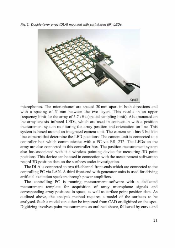
microphones. The microphones are spaced 30 mm apart in both directions andwith a spacing of 31 mm between the two layers. This results in an upperfrequency limit for the array of 5.7 kHz (spatial sampling limit). Also mounted onthe array are six infrared LEDs, which are used in connection with a positionmeasurement system monitoring the array position and orientation on-line. Thissystem is based around an integrated camera unit. The camera unit has 3 built-inline cameras that determine the LED positions. The camera unit is connected to acontroller box which communicates with a PC via RS–232. The LEDs on thearray are also connected to this controller box. The position measurement systemalso has associated with it a wireless pointing device for measuring 3D pointpositions. This device can be used in connection with the measurement software torecord 3D position data on the surfaces under investigation.

The DLA is connected to two 65-channel front-ends which are connected to thecontrolling PC via LAN. A third front-end with generator units is used for drivingartificial excitation speakers through power amplifiers.

The controlling PC is running measurement software with a dedicatedmeasurement template for acquisition of array microphone signals andcorresponding array positions in space, as well as surface point position data. Asoutlined above, the analysis method requires a model of the surfaces to beanalysed. Such a model can either be imported from CAD or digitized on the spot.Digitizing involves point measurements as outlined above, followed by curve and

Fig. 3. Double-layer array (DLA) mounted with six infrared (IR) LEDs

21

surface construction. In both cases, the end result is a CAD-type parametricsurface description which is later used as the basis for creating a surface mesh.This mesh is in turn used for calculation and results display.

Measurement ProcedureThe DLA is placed in positions close to the surfaces under investigation to samplethe near field sound pressure. The position of the array is recorded online via theposition measurement system and microphone time histories are recorded for eacharray position. The array is placed in slightly overlapping positions to cover theinvestigated surfaces patch by patch. The data acquisition software displays thecurrent and past array positions in 3D along with the surface model. In this waythe user can identify which parts of the surface have been covered with the arrayand which parts still need to be covered.

When measuring for the estimation of surface absorption, a number ofloudspeakers are distributed in the cabin interior and driven by uncorrelated noisesources, to create a distributed and (close-to) diffuse excitation field. Measurementfor the actual estimation of entering intensity is, of course, performed in operatingconditions with these sources turned off. All recorded data are stored to a database.

Data ProcessingThe post-processing software application retrieves all data from the database. Asurface mesh is created based on the parametric surface description. A number ofmesh areas may be defined in this process. These can be used for averaging of, forexample, absorption coefficient.

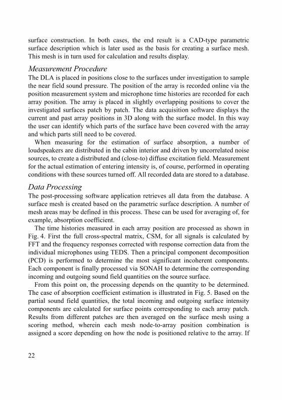
The time histories measured in each array position are processed as shown inFig. 4. First the full cross-spectral matrix, CSM, for all signals is calculated byFFT and the frequency responses corrected with response correction data from theindividual microphones using TEDS. Then a principal component decomposition(PCD) is performed to determine the most significant incoherent components.Each component is finally processed via SONAH to determine the correspondingincoming and outgoing sound field quantities on the source surface.

From this point on, the processing depends on the quantity to be determined.The case of absorption coefficient estimation is illustrated in Fig. 5. Based on thepartial sound field quantities, the total incoming and outgoing surface intensitycomponents are calculated for surface points corresponding to each array patch.Results from different patches are then averaged on the surface mesh using ascoring method, wherein each mesh node-to-array position combination isassigned a score depending on how the node is positioned relative to the array. If

22

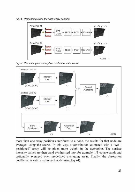
more than one array position contributes to a node, the results for that node areaveraged using the scores. In this way, a contribution estimated with a “well-positioned” array will be given more weight in the averaging. The surfaceintensity values are then band-synthesised into, for example, 1/3-octave bands andoptionally averaged over predefined averaging areas. Finally, the absorptioncoefficient is estimated in each node using Eq. (4).

Fig. 4. Processing steps for each array position

Fig. 5. Processing for absorption coefficient estimation

Array Pos #1

Array Pos #2

FFTCSM TEDS PCD SONAH

FFTCSM TEDS PCD SONAH

(p–,u–)(p+,u+),

(p–,u–)(p+,u+),

100148

(p–,u–)(p+,u+),

(p–,u–)(p+,u+),

I+,I–

I+,I–

I+,I–

I+,I– α

Surface Data #1

Surface Data #2

IntensityCalc.

IntensityCalc.

ScoredAveraging

BandSynthesis

AbsorptionCalc.

100149

23

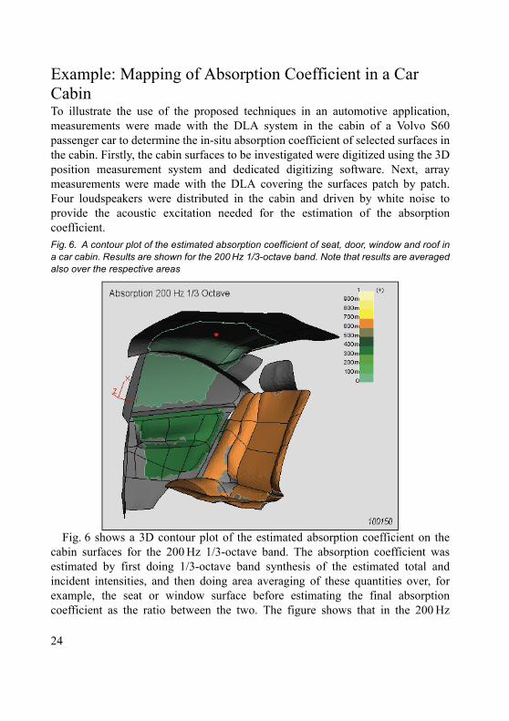
Example: Mapping of Absorption Coefficient in a Car CabinTo illustrate the use of the proposed techniques in an automotive application,measurements were made with the DLA system in the cabin of a Volvo S60passenger car to determine the in-situ absorption coefficient of selected surfaces inthe cabin. Firstly, the cabin surfaces to be investigated were digitized using the 3Dposition measurement system and dedicated digitizing software. Next, arraymeasurements were made with the DLA covering the surfaces patch by patch.Four loudspeakers were distributed in the cabin and driven by white noise toprovide the acoustic excitation needed for the estimation of the absorptioncoefficient.

Fig. 6 shows a 3D contour plot of the estimated absorption coefficient on thecabin surfaces for the 200 Hz 1/3-octave band. The absorption coefficient wasestimated by first doing 1/3-octave band synthesis of the estimated total andincident intensities, and then doing area averaging of these quantities over, forexample, the seat or window surface before estimating the final absorptioncoefficient as the ratio between the two. The figure shows that in the 200 Hz

Fig. 6. A contour plot of the estimated absorption coefficient of seat, door, window and roof ina car cabin. Results are shown for the 200 Hz 1/3-octave band. Note that results are averagedalso over the respective areas

24

frequency band, the seat has quite a high absorption coefficient compared to thedoor, window and roof.

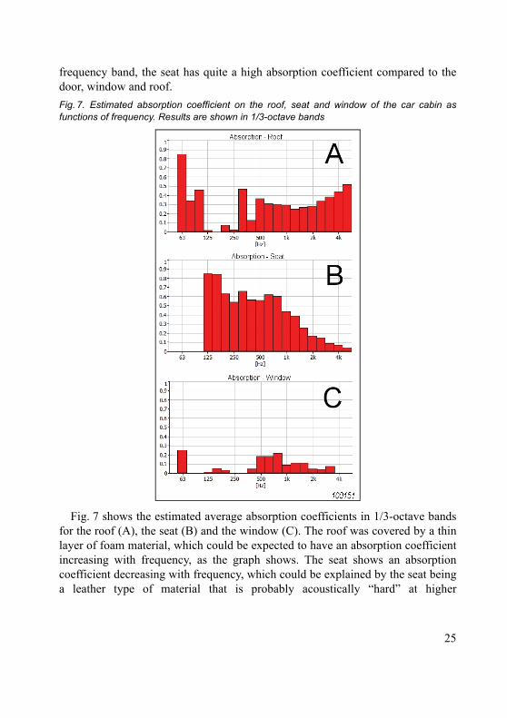
Fig. 7 shows the estimated average absorption coefficients in 1/3-octave bandsfor the roof (A), the seat (B) and the window (C). The roof was covered by a thinlayer of foam material, which could be expected to have an absorption coefficientincreasing with frequency, as the graph shows. The seat shows an absorptioncoefficient decreasing with frequency, which could be explained by the seat beinga leather type of material that is probably acoustically “hard” at higher

Fig. 7. Estimated absorption coefficient on the roof, seat and window of the car cabin asfunctions of frequency. Results are shown in 1/3-octave bands

25

frequencies. Finally, the window shows quite a low absorption coefficientthroughout the whole frequency range under investigation, as could be expected.

ConclusionA method for measuring the absorption coefficient, radiated and absorbedintensity on the panels of a vehicle cabin has been described and it was shown howthe method can be used to map, for example, the absorption coefficient on theinterior surfaces of a car cabin. The method is based on a Dual Layer Array withintegrated position measurement. The method has shown good ability to determinethe actual radiated sound intensity in the presence of a diffuse field in the cabin.

AknowledgementsThis paper is based on work done in the European Union research project Cabinnoise Reduction by Experimental and numerical Design Optimization, CREDO,which deals with noise in aircraft and helicopter cabins. Since the radiatedintensity is often seen from the perspective of the cabin, it is sometimes also calledEntering Intensity (EI) [4]. Simulations as well as results of measurement insideaircraft can be found in [4, 7].

26

References[1] Hardy, P., Trentin, D., Jézéquel, L., Ichchou, M. N., “Identification of noise

sources in an in-flight aircraft by means of local energy method ”;Proceedings of Euronoise 2006.

[2] Hald, J., “STSF – a unique technique for scan-based Near-field AcousticalHolography without restrictions on coherence”; Brüel & Kjær TechnicalReview, No. 1, 1989.

[3] Hald, J., “Patch holography in cabin environments using a two-layerhandheld array with an extended SONAH algorithm”; Proceedings ofEuronoise 2006.

[4] Hald, J., Mørkholt, J., “Methods to estimate the Entering Intensity and theirimplementation using SONAH ”; Report DWP 2.3 from the Europeanproject CREDO, 2007.

[5] Alvarez, J. D., Jacobsen, F., “In-situ measurements of the complex acousticimpedance of porous materials”; Proceedings of Inter-Noise 2007

[6] Hald, J., Mørkholt, J., “Array based Measurement of Radiated andAbsorbed Sound Intensity Components”; Proc. Acoustics ’08, 2008

[7] Hald, J., Mørkholt, J., Hardy, P., Trentin, D., Bach-Andersen, M., Keith, G.,“Measurement of Absorption Coefficient, Surface Admittance, RadiatedIntensity and Absorbed Intensity on the Panels of a Vehicle Cabin using aDual Layer Array with Integrated Position Measurement ”; Proceedings ofSAE, 2009

27

ISO 16063–11: Uncertainties in Primary Vibration Calibration by Laser Interferometry – Reference Planes and Transverse Motion*

Torben Licht and Sven Erik Salbøl

AbstractPrimary vibration calibration by laser interferometry using quadrature outputs hasbeen used for the last 10 to 15 years. ISO 16063–11 [1] was published in 1999 andhas increased the interest further. With the advent of new compact laserinterferometers, the difficulties of optical alignment and adjustment have beenpractically eliminated, and dedicated software has made the process automatic,which facilitates collection of much more data.

In most cases the method is applied to reference transducers, either single-endedor those meant for back-to-back calibration. Because the laser beam cannot alwaysbe directed towards an ideal point or surface, significant errors can be introduced.At low frequencies this is often due to non-ideal exciter motions. At highfrequencies it is often due to relative motion between points on apparently rigidmechanical structures, or rocking or bending motion of the combined structures.Some examples and solutions to these problems, including uncertaintycalculations, will be presented in this paper.

RésuméL’étalonnage primaire de vibrations par interférométrie laser avec sortie enquadrature est utilisé depuis une quinzaine d’années. La Norme ISO 16063–11 [1]publiée en 1999 connaît un intérêt croissant. Avec l’arrivée de nouveauxinterféromètres de laser très compacts, les difficultés liées au réglage et àl’alignement optique ont été pratiquement éliminées, et des logiciels dédiés ontautomatisé les procédures, facilitant l’acquisition d’une plus grande quantité dedonnées.

* First published at IMEKO XIX World Congress: Fundamental and Applied Technology, Lisbon,Portugal

28

Dans la plupart des cas, cette méthode est appliquée pour les capteurs deréférence, qu’ils soient accélerometre de transfert monobase ou destinés àl’étalonnage dos-à-dos. Comme le faisceau laser ne peut pas toujours être dirigévers un point ou une surface idéal(e), des erreurs non négligeables peuventapparaître. Aux basses fréquences, cela est souvent dû à un mouvement non idéalde l’excitateur. Aux hautes fréquences, au déplacement relatif entre points sur desstructures mécaniques apparemment rigides, ou au balancement ou fléchissementde structures combinées. La présente communication exemplifie ces problèmes etleurs solutions, y compris les calculs de l’incertitude.

ZusammenfassungPrimärkalibrierung von Schwingungssensoren durch Laserinterferometrie mitQuadraturausgängen wird seit ca. 10 – 15 Jahren verwendet. Die 1999veröffentlichte ISO 16063–11 [1] hat das Interesse weiter gesteigert. Mit denneuen kompakten Laserinterferometern wurden die Schwierigkeiten bei deroptischen Ausrichtung und Justierung in der Praxis eliminiert. DurchSpezialsoftware wurde der Prozess automatisch gemacht, so dass sich heutewesentlich mehr Daten sammeln lassen.

In den meisten Fällen wird die Methode auf Bezugsnormalsensoren angewendet,entweder single-ended oder solche, die für Back-to-Back-Kalibrierung vorgesehensind. Da sich der Laserstrahl nicht immer auf einen idealen Punkt oder eine idealeFläche richten lässt, können wesentliche Fehler entstehen. Bei tiefen Frequenzensind diese häufig auf nichtideale Bewegungen des Schwingerregerszurückzuführen, bei hohen Frequenzen dagegen auf die Relativbewegungzwischen Punkten auf scheinbar steifen mechanischen Strukturen oder aufSchaukel- oder Biegebewegungen der kombinierten Strukturen. In diesem Artikelwerden einige Beispiele und Lösungen für diese Probleme vorgestellt, darunterUnsicherheitsberechnungen.

IntroductionISO 16063–11, Methods for the Calibration of Vibration and Shock Transducers –Part 11: Primary Vibration Calibration by Laser Interferometry, does not go intomuch detail when the quality of the motion is described. The standard states:

“Transverse, bending and rocking acceleration: Sufficiently small to preventexcessive effects on the calibration results. At large amplitudes, preferably in the

29

low-frequency range from 1 Hz to 10 Hz, transverse motion of less than 1 % of themotion in the intended direction may be required; above 10 Hz to 1 kHz, amaximum of 10 % of the axial motion is permitted; above 1 kHz, a maximum of20% of the axial motion is tolerated.”

About the calibration of back-to-back accelerometers it states:“Typically, a 20 g mass is used. The laser light spot can be at either the top

(outer surface) of the dummy mass or the top surface of the referenceaccelerometer.

If the motion is sensed at the top of the dummy mass, then the dummy massshould have an optically polished top surface, and the position of the laser-lightspot should be close to the geometrical centre of this surface. In cases where themotion of the mass departs from that of a rigid body, the relative motion betweenthe top (sensed) and bottom surfaces shall be taken into consideration. To simulatea mass of 20 g of typical transfer standard accelerometers, a dummy mass in theform of a hexagonal steel bar 12 mm in length and 16 mm in width over flats ofhexagonal faces can be used. At a frequency of 5 kHz, for example, the relativemotion introduces systematic errors of 0.26 % in amplitude measurements and4.2° in phase shift measurements”.

The standard also states uncertainties attainable as:“For the magnitude of sensitivity:0.5 % of the measured value at reference conditions;< 1 % of the measured value outside reference conditions.”The standard was mainly written to help national metrology institutes (and

similar laboratories) to work in similar ways. These have, since the publication ofthe standard, claimed far better uncertainties (0.1 to 0.5 % in the full frequencyrange).

In these cases, the motion has normally been measured at the reference surfaceof the reference accelerometer, and a slotted mass has been used.

This means that the point(s) at which the motion is measured by theinterferometer are positioned at a distance of some millimetres from the centre.This makes the transverse motion, which is normally a rocking motion, a majorcontributor to the uncertainty.

To avoid this, a dummy mass, as described above, can be used and the motionmeasured at the centre. However, this leaves the problem of estimating (with greataccuracy) the motion at the interface between the dummy mass and the referenceaccelerometer.

30

Transverse Motion of ExcitersManufacturers of exciters do sometimes give specifications for transverse motion,but the way these are obtained is rarely given and they are probably measuredusing mostly small, carefully symmetrical loads, placed directly on top of themoving element. Therefore, an investigation of actual transverse motion wasperformed on three different exciters. One was a classical spring controlled model,the other two were air-bearing exciters with a specified low transverse motion.

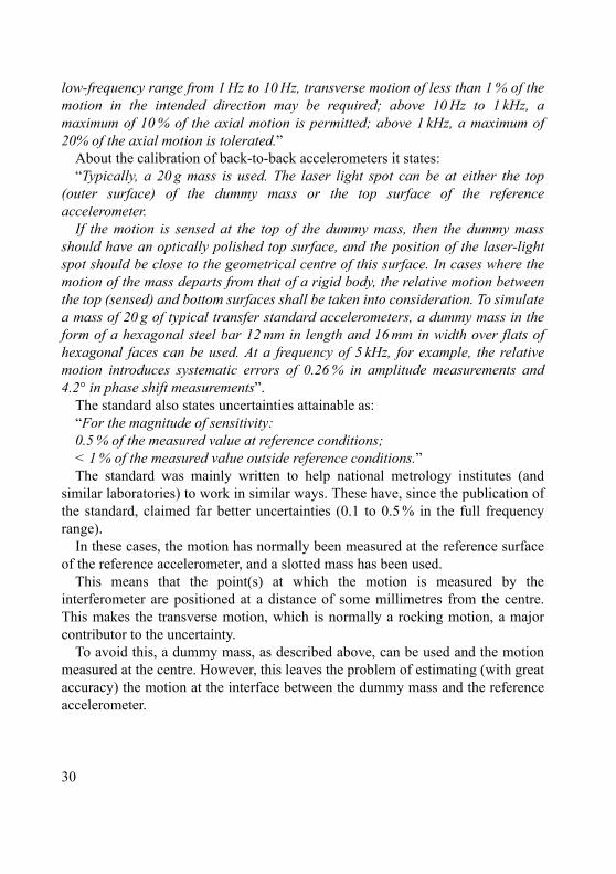
Exciters A and B are air-bearing types; exciter C is a classical spring type.Measurements on A and B were made orthogonal to the excitation direction in twodifferent directions (X and Y, 120 degrees apart) at the top end of a referencetransducer (Brüel & Kjær Type 8305), with a 20 gram slotted load-mass at themounting surface of the accelerometer (Fig. 1). (The slotted load-mass is of PTBdesign and is normally used for laser interferometry, Fig. 24.) On exciter C, Type8305 was loaded with a cubic 30 gram block with four identical accelerometersmounted on its surfaces to measure the transverse motion (Fig. 2). Measurementsfrom two accelerometers orthogonal to each other are made use of.

The results are plotted in three groups: Figs. 3 – 8 are for exciter A, Figs. 9 – 14for exciter B, and Figs. 15 – 20 for exciter C. The excitation was a random signaland the spectrum obtained as measured by the Type 8305 is shown in the bottomleft-hand graph for each of the three groups mentioned above. The transversemotions relative to the main direction for each shaker are shown as the first twocurves on the left-hand side of each group. The maximum on the graphscorresponds to 100% transverse motion. From the results, it became clear that thespecifications for transverse motion are not useful for estimating the motion anduncertainties related to transverse motion when a back-to-back referencetransducer is mounted directly on top of the exciter table. The combined structureof the exciter table and the reference transducer shows high transverse levels in the

Fig. 1. Slotted mass on Type 8305 Fig. 2. Cubic block on Type 8305

31

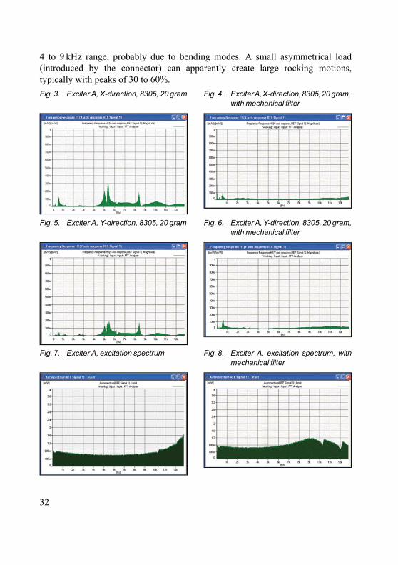
4 to 9 kHz range, probably due to bending modes. A small asymmetrical load(introduced by the connector) can apparently create large rocking motions,typically with peaks of 30 to 60%.

Fig. 3. Exciter A, X-direction, 8305, 20 gram Fig. 4. Exciter A, X-direction, 8305, 20 gram, with mechanical filter

Fig. 5. Exciter A, Y-direction, 8305, 20 gram Fig. 6. Exciter A, Y-direction, 8305, 20 gram,with mechanical filter

Fig. 7. Exciter A, excitation spectrum Fig. 8. Exciter A, excitation spectrum, withmechanical filter

32

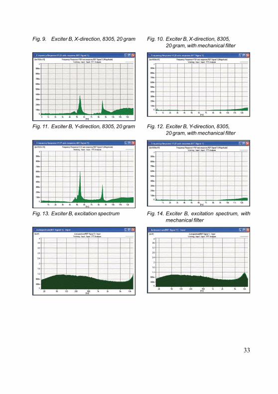
Fig. 9. Exciter B, X-direction, 8305, 20 gram Fig. 10. Exciter B, X-direction, 8305,20 gram, with mechanical filter

Fig. 11. Exciter B, Y-direction, 8305, 20 gram Fig. 12. Exciter B, Y-direction, 8305,20 gram, with mechanical filter

Fig. 13. Exciter B, excitation spectrum Fig. 14. Exciter B, excitation spectrum, withmechanical filter

33

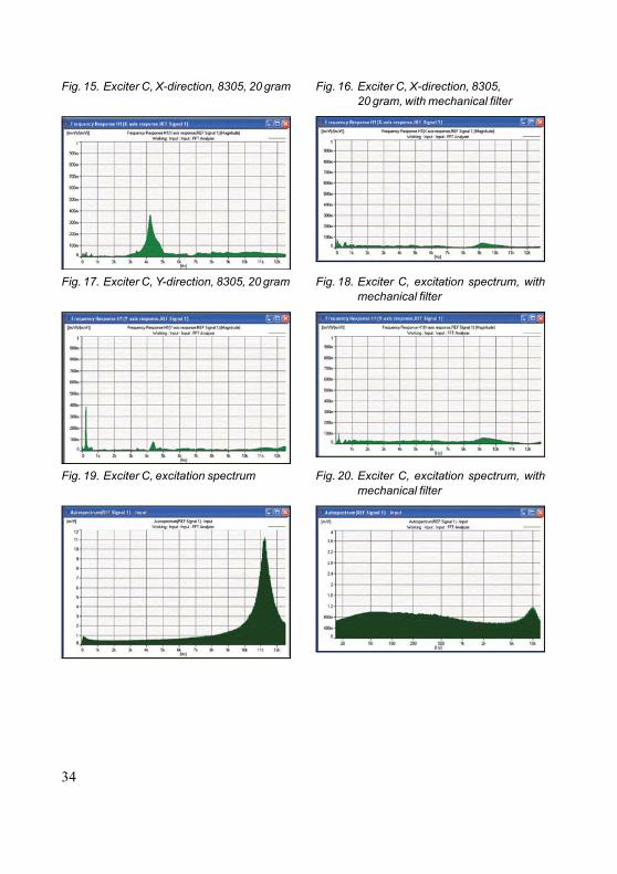
Fig. 15. Exciter C, X-direction, 8305, 20 gram Fig. 16. Exciter C, X-direction, 8305, 20 gram, with mechanical filter

Fig. 17. Exciter C, Y-direction, 8305, 20 gram Fig. 18. Exciter C, excitation spectrum, withmechanical filter

Fig. 19. Exciter C, excitation spectrum Fig. 20. Exciter C, excitation spectrum, withmechanical filter

34

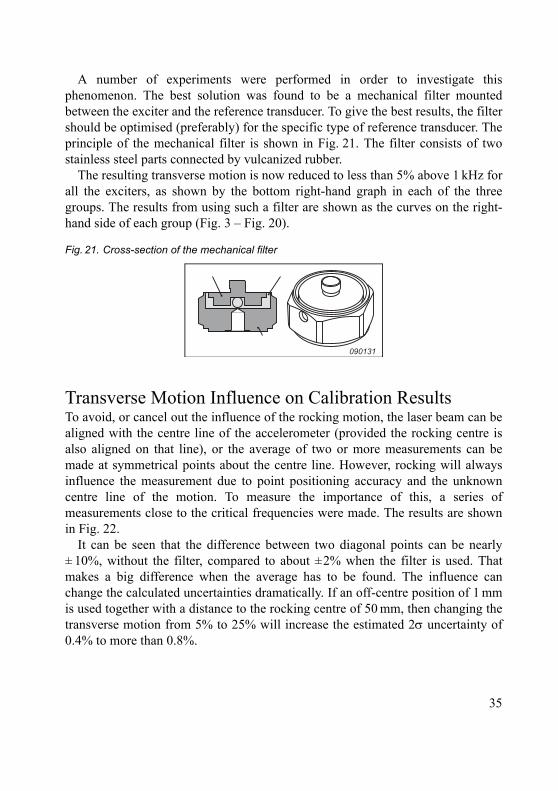
A number of experiments were performed in order to investigate thisphenomenon. The best solution was found to be a mechanical filter mountedbetween the exciter and the reference transducer. To give the best results, the filtershould be optimised (preferably) for the specific type of reference transducer. Theprinciple of the mechanical filter is shown in Fig. 21. The filter consists of twostainless steel parts connected by vulcanized rubber.

The resulting transverse motion is now reduced to less than 5% above 1 kHz forall the exciters, as shown by the bottom right-hand graph in each of the threegroups. The results from using such a filter are shown as the curves on the right-hand side of each group (Fig. 3 – Fig. 20).

Transverse Motion Influence on Calibration ResultsTo avoid, or cancel out the influence of the rocking motion, the laser beam can bealigned with the centre line of the accelerometer (provided the rocking centre isalso aligned on that line), or the average of two or more measurements can bemade at symmetrical points about the centre line. However, rocking will alwaysinfluence the measurement due to point positioning accuracy and the unknowncentre line of the motion. To measure the importance of this, a series ofmeasurements close to the critical frequencies were made. The results are shownin Fig. 22.

It can be seen that the difference between two diagonal points can be nearly± 10%, without the filter, compared to about ±2% when the filter is used. Thatmakes a big difference when the average has to be found. The influence canchange the calculated uncertainties dramatically. If an off-centre position of 1 mmis used together with a distance to the rocking centre of 50 mm, then changing thetransverse motion from 5% to 25% will increase the estimated 2 uncertainty of0.4% to more than 0.8%.

Fig. 21. Cross-section of the mechanical filter

090131

35

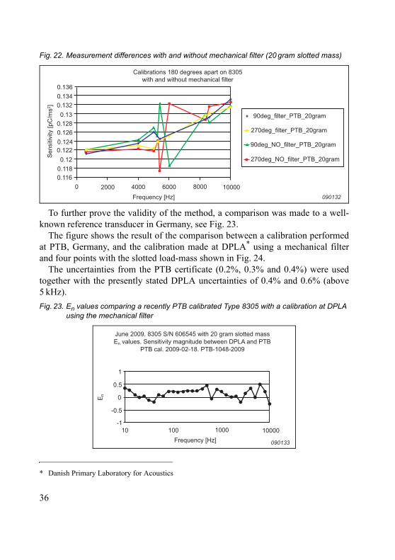
To further prove the validity of the method, a comparison was made to a well-known reference transducer in Germany, see Fig. 23.

The figure shows the result of the comparison between a calibration performedat PTB, Germany, and the calibration made at DPLA* using a mechanical filterand four points with the slotted load-mass shown in Fig. 24.

The uncertainties from the PTB certificate (0.2%, 0.3% and 0.4%) were usedtogether with the presently stated DPLA uncertainties of 0.4% and 0.6% (above5 kHz).

Fig. 22. Measurement differences with and without mechanical filter (20 gram slotted mass)

* Danish Primary Laboratory for Acoustics

Fig. 23. En values comparing a recently PTB calibrated Type 8305 with a calibration at DPLA using the mechanical filter

090132

0.1360.1340.1320.13

0.1280.1260.1240.1220.12

0.1180.116

0 2000 4000 6000 8000 10000Frequency [Hz]

Sen

sitiv

ity [p

C/m

s2 ]

Calibrations 180 degrees apart on 8305with and without mechanical filter

90deg_filter_PTB_20gram

270deg_filter_PTB_20gram

90deg_NO_filter_PTB_20gram

270deg_NO_filter_PTB_20gram

June 2009. 8305 S/N 606545 with 20 gram slotted massEn values. Sensitivity magnitude between DPLA and PTB

PTB cal. 2009-02-18. PTB-1048-2009

090133Frequency [Hz]

En

1000010 100 1000

1

0.5

0

-0.5

-1

36

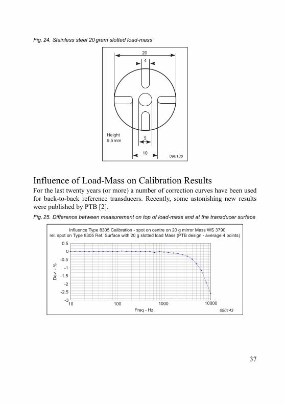
Influence of Load-Mass on Calibration ResultsFor the last twenty years (or more) a number of correction curves have been usedfor back-to-back reference transducers. Recently, some astonishing new resultswere published by PTB [2].

Fig. 24. Stainless steel 20 gram slotted load-mass

Fig. 25. Difference between measurement on top of load-mass and at the transducer surface

20

4

5

10

Height9.5 mm

090130

Influence Type 8305 Calibration - spot on centre on 20 g mirror Mass WS 3790 rel. spot on Type 8305 Ref. Surface with 20 g slotted load Mass (PTB design - average 4 points)

0.5

0

-0.5

Dev

. - %

-1

-1.5

-2

-2.5

-3 10 100

Freq - Hz1000 10000

090143

37

At DPLA a number of measurements were undertaken to question and verifythese new results. One of the first measurements was to compare the results on topof a 20 gram solid stainless steel mass (as described in the standard [1]), to theresults obtained at the interface between the transducer and a slotted 20 grammass. The difference is shown in Fig. 25, and this shows a deviation well beyondthe value stated in the standard.

A number of measurements similar to the results reported in [2] are in theprocess of being completed, but these seem to confirm the findings.

ConclusionsThe transverse motion of different shakers has been investigated. The results showthat even high quality shakers designed for calibration show very high levels oftransverse motion at higher frequencies, when back-to-back accelerometers withload-masses are mounted on them. This is detrimental to the laser-interferometricmeasurements used to give the best possible primary calibrations.

A solution to this problem has been devised in the form of mechanical filters,which modify the assembly to remove the high frequency bending modes of theshaker plus accelerometer structure.

The use of slotted load-masses for calibration of back-to-back accelerometershas been taken up, and it has been shown that the difference between this and theoften used mirror-masses is much larger than normally expected. This is thesubject of further work and discussion.

References[1] ISO 16063–11, “Methods for the Calibration of Vibration and Shock

Transducers – Part 11: Primary Vibration Calibration by LaserInterferometry”, 1999.

[2] Täubner, A., Schlaak, H-J., Bruns, T., “Metrological and TheoreticalInvestigations of the Influence of Mass Loads on the TransmissionCoefficient of Acceleration Transducers of the Back-to-back Type”,Physikalisch Technische Bundesanstalt, 38116 Braunschweig, Germany.

38

Previously issued numbers ofBrüel & Kjær Technical Review1 – 2009 Use of Volume Velocity Sound Sources in the Measurement of Acoustic

Frequency Response FunctionsTurnkey Free-field Reciprocity System for Primary Microphone Calibration

1 – 2008 ISO 16063–11: Primary Vibration Calibration by Laser Interferometry: Evaluation of Sine Approximation Realised by FFTInfrasound Calibration of Measurement MicrophonesImproved Temperature Specifications for Transducers with Built-in Electronics

1 – 2007 Measurement of Normal Incidence Transmission Loss and Other Acoustical Properties of Materials Placed in a Standing Wave Tube

1 – 2006 Dyn-X Technology: 160 dB in One Input RangeOrder Tracking in Vibro-acoustic Measurements: A Novel ApproachEliminating the Tacho ProbeComparison of Acoustic Holography Methods for Surface Velocity Determination on a Vibrating Panel

1 – 2005 Acoustical Solutions in the Design of a Measurement Microphone for Surface MountingCombined NAH and Beamforming Using the Same ArrayPatch Near-field Acoustical Holography Using a New Statistically Optimal Method

1 – 2004 Beamforming1 – 2002 A New Design Principle for Triaxial Piezoelectric Accelerometers

Use of FE Models in the Optimisation of Accelerometer DesignsSystem for Measurement of Microphone Distortion and Linearity from Medium to Very High Levels

1 – 2001 The Influence of Environmental Conditions on the Pressure Sensitivity of Measurement MicrophonesReduction of Heat Conduction Error in Microphone Pressure Reciprocity CalibrationFrequency Response for Measurement Microphones – a Question of ConfidenceMeasurement of Microphone Random-incidence and Pressure-field Responses and Determination of their Uncertainties

1 – 2000 Non-stationary STSF1 – 1999 Characteristics of the Vold-Kalman Order Tracking Filter1 – 1998 Danish Primary Laboratory of Acoustics (DPLA) as Part of the National

Metrology OrganisationPressure Reciprocity Calibration – Instrumentation, Results and UncertaintyMP.EXE, a Calculation Program for Pressure Reciprocity Calibration of Microphones

(Continued on cover page 3)

1 – 1997 A New Design Principle for Triaxial Piezoelectric AccelerometersA Simple QC Test for Knock SensorsTorsional Operational Deflection Shapes (TODS) Measurements

2 – 1996 Non-stationary Signal Analysis using Wavelet Transform, Short-time Fourier Transform and Wigner-Ville Distribution

1 – 1996 Calibration Uncertainties & Distortion of Microphones.Wide Band Intensity Probe. Accelerometer Mounted Resonance Test

2 – 1995 Order Tracking Analysis1 – 1995 Use of Spatial Transformation of Sound Fields (STSF) Techniques in the

Automative Industry2 – 1994 The use of Impulse Response Function for Modal Parameter Estimation

Complex Modulus and Damping Measurements using Resonant and Non-resonant Methods (Damping Part II)

1 – 1994 Digital Filter Techniques vs. FFT Techniques for Damping Measurements (Damping Part I)

2 – 1990 Optical Filters and their Use with the Type 1302 & Type 1306 Photoacoustic Gas Monitors

1 – 1990 The Brüel & Kjær Photoacoustic Transducer System and its Physical Properties

2 – 1989 STSF – Practical Instrumentation and ApplicationDigital Filter Analysis: Real-time and Non Real-time Performance

1 – 1989 STSF – A Unique Technique for Scan Based Near-Field Acoustic Holography Without Restrictions on Coherence

2 – 1988 Quantifying Draught Risk1 – 1988 Using Experimental Modal Analysis to Simulate Structural Dynamic

ModificationsUse of Operational Deflection Shapes for Noise Control of Discrete Tones

Special technical literatureBrüel & Kjær publishes a variety of technical literature which can be obtained from your local Brüel & Kjær representative.

The following literature is presently available:

• Catalogues (several languages)• Product Data Sheets (English, German, French,)

Furthermore, back copies of the Technical Review can be supplied as listed above. Older issues may be obtained provided they are still in stock.

Previously issued numbers ofBrüel & Kjær Technical Review(Continued from cover page 2)

TECHNICAL REVIEWNo. 1 – 2010

HEADQUARTERS: Brüel & Kjær Sound & Vibration Measurement A/S DK-2850 Nærum Denmark · Telephone: +45 7741 2000 · Fax: +45 4580 1405 www.bksv.com · info@bksv.com

Local representatives and service organisations worldwide

BV00

62–

11IS

SN00

07–

2621

ËBV-0062---'Î

Time Selective Response MethodIn situ Measurement of Absorption Coefficient

Transverse Motion in Accelerometer Calibration