Embed Size (px)
Citation preview
Business Statistics: A Decision-Making Approach, 6e © 2005 Prentice-Hall, Inc. Chap 8-1
Business Statistics: A Decision-Making Approach
6th Edition
Chapter 8Introduction to
Hypothesis Testing
Business Statistics: A Decision-Making Approach, 6e © 2005 Prentice-Hall, Inc. Chap 8-2
Chapter Goals
After completing this chapter, you should be able to:
Formulate null and alternative hypotheses for applications involving a single population mean or proportion
Formulate a decision rule for testing a hypothesis Know how to use the test statistic, critical value, and
p-value approaches to test the null hypothesis Know what Type I and Type II errors are Compute the probability of a Type II error
Business Statistics: A Decision-Making Approach, 6e © 2005 Prentice-Hall, Inc. Chap 8-3
What is a Hypothesis?
A hypothesis is a claim (assumption) about a population parameter:
population mean
population proportion
Example: The mean monthly cell phone bill of this city is = $42
Example: The proportion of adults in this city with cell phones is p = .68
Business Statistics: A Decision-Making Approach, 6e © 2005 Prentice-Hall, Inc. Chap 8-4
The Null Hypothesis, H0
States the assumption (numerical) to be tested
Example: The average number of TV sets in
U.S. Homes is at least three ( )
Is always about a population parameter, not about a sample statistic
3μ:H0
3μ:H0 3x:H0
Business Statistics: A Decision-Making Approach, 6e © 2005 Prentice-Hall, Inc. Chap 8-5
The Null Hypothesis, H0
Begin with the assumption that the null hypothesis is true Similar to the notion of innocent until
proven guilty Refers to the status quo Always contains “=” , “≤” or “” sign May or may not be rejected
(continued)
Business Statistics: A Decision-Making Approach, 6e © 2005 Prentice-Hall, Inc. Chap 8-6
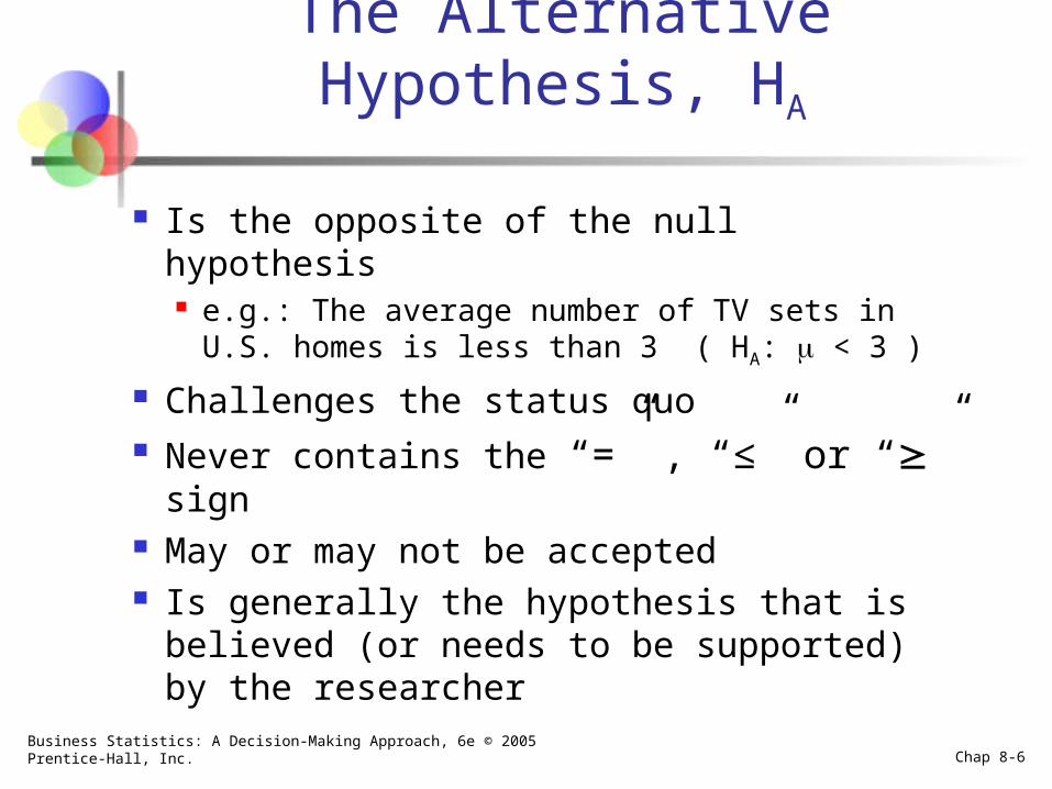
The Alternative Hypothesis, HA
Is the opposite of the null hypothesis e.g.: The average number of TV sets in U.S.
homes is less than 3 ( HA: < 3 )
Challenges the status quo Never contains the “=” , “≤” or “” sign May or may not be accepted Is generally the hypothesis that is believed
(or needs to be supported) by the researcher
Business Statistics: A Decision-Making Approach, 6e © 2005 Prentice-Hall, Inc.
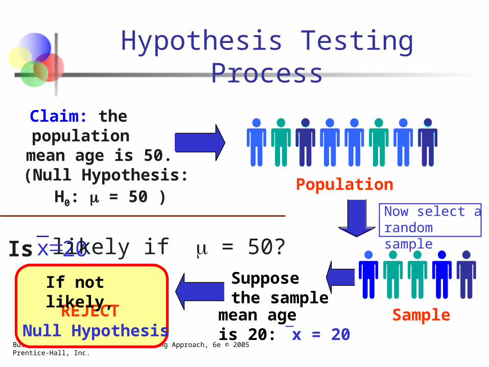
Population
Claim: thepopulationmean age is 50.(Null Hypothesis:
REJECT
Supposethe samplemean age is 20: x = 20
SampleNull Hypothesis
20 likely if = 50?Is
Hypothesis Testing Process
If not likely,
Now select a random sample
H0: = 50 )
x
Business Statistics: A Decision-Making Approach, 6e © 2005 Prentice-Hall, Inc. Chap 8-8
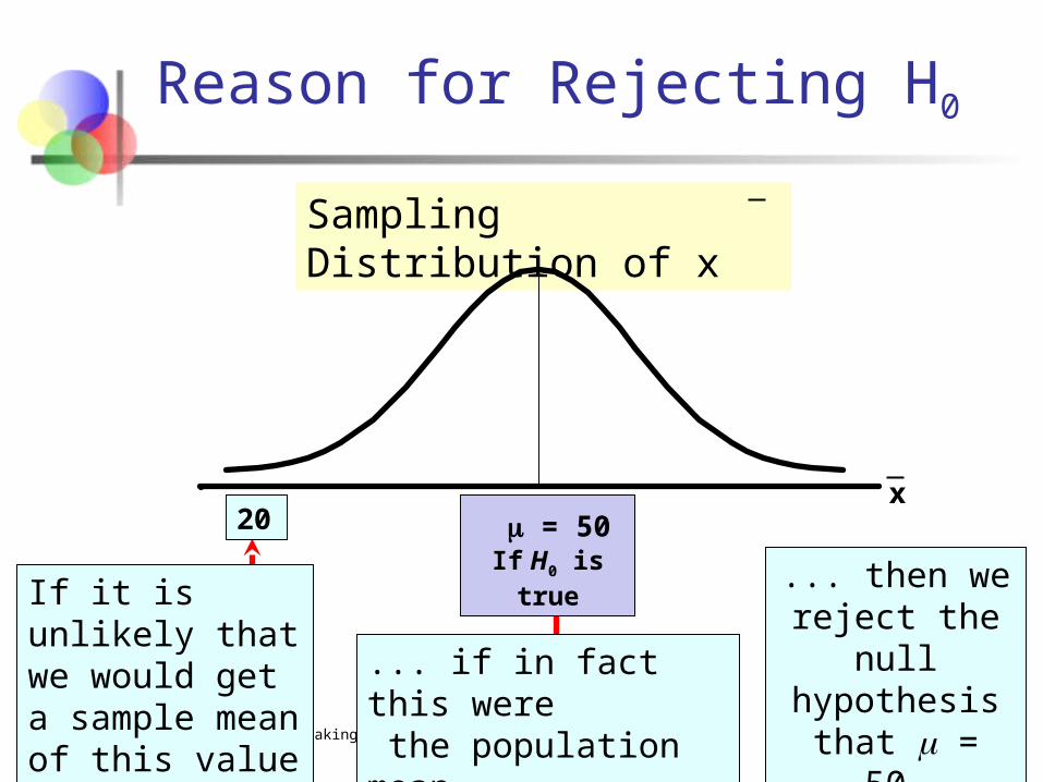
Sampling Distribution of x
= 50If H0 is true
If it is unlikely that we would get a sample mean of this value ...
... then we reject the null
hypothesis that = 50.
Reason for Rejecting H0
20
... if in fact this were the population mean…
x
Business Statistics: A Decision-Making Approach, 6e © 2005 Prentice-Hall, Inc. Chap 8-9
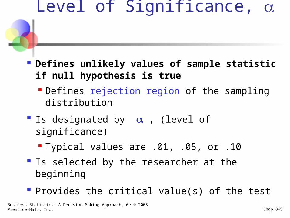
Level of Significance,
Defines unlikely values of sample statistic if null hypothesis is true Defines rejection region of the sampling
distribution
Is designated by , (level of significance) Typical values are .01, .05, or .10
Is selected by the researcher at the beginning
Provides the critical value(s) of the test
Business Statistics: A Decision-Making Approach, 6e © 2005 Prentice-Hall, Inc. Chap 8-10
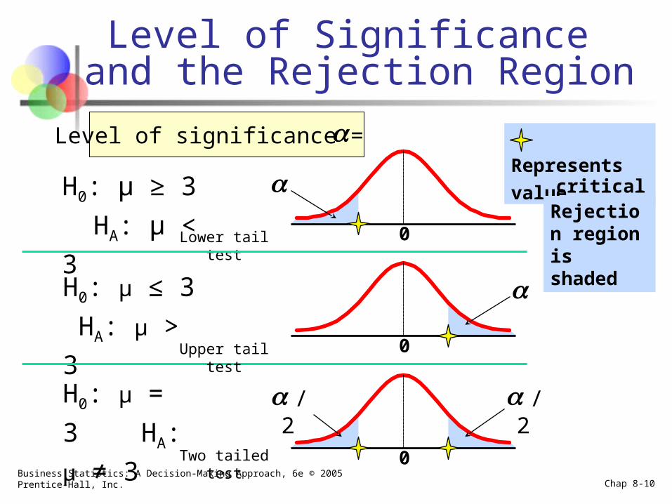
Level of Significance and the Rejection Region
H0: μ ≥ 3
HA: μ < 3 0
H0: μ ≤ 3
HA: μ > 3
H0: μ = 3
HA: μ ≠ 3
/2
Represents critical value
Lower tail test
Level of significance =
0
0
/2
Upper tail test
Two tailed test
Rejection region is shaded
Business Statistics: A Decision-Making Approach, 6e © 2005 Prentice-Hall, Inc. Chap 8-11
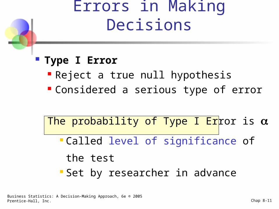
Errors in Making Decisions
Type I Error Reject a true null hypothesis Considered a serious type of error
The probability of Type I Error is Called level of significance of the test Set by researcher in advance
Business Statistics: A Decision-Making Approach, 6e © 2005 Prentice-Hall, Inc. Chap 8-12
Errors in Making Decisions
Type II Error Fail to reject a false null hypothesis
The probability of Type II Error is β
(continued)
Business Statistics: A Decision-Making Approach, 6e © 2005 Prentice-Hall, Inc. Chap 8-13
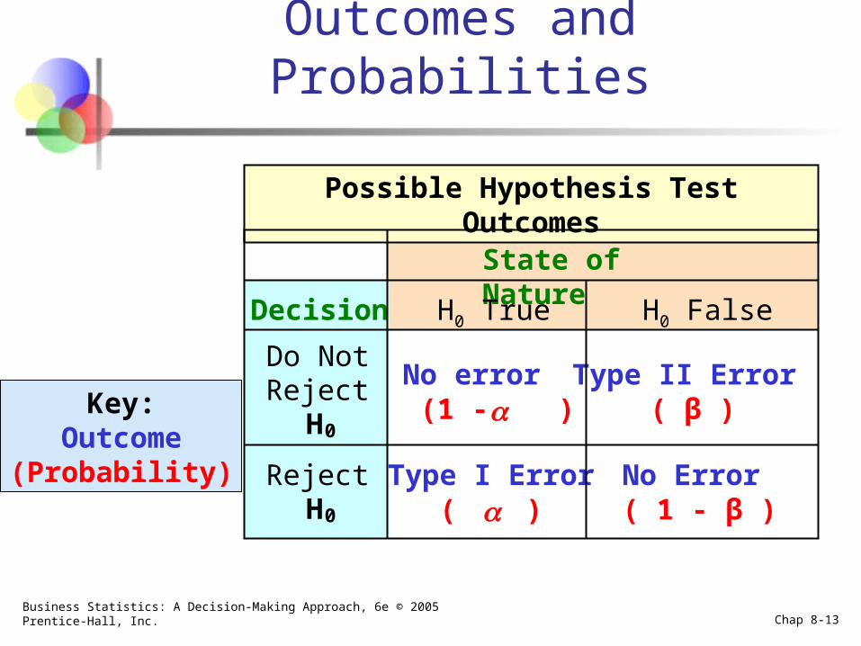
Outcomes and Probabilities
State of Nature
Decision
Do NotReject
H0
No error (1 - )
Type II Error ( β )
RejectH0
Type I Error( )
Possible Hypothesis Test Outcomes
H0 False H0 True
Key:Outcome
(Probability) No Error ( 1 - β )
Business Statistics: A Decision-Making Approach, 6e © 2005 Prentice-Hall, Inc. Chap 8-14
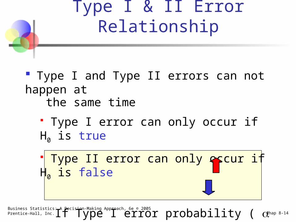
Type I & II Error Relationship
Type I and Type II errors can not happen at the same time
Type I error can only occur if H0 is true
Type II error can only occur if H0 is false
If Type I error probability ( ) , then
Type II error probability ( β )
Business Statistics: A Decision-Making Approach, 6e © 2005 Prentice-Hall, Inc. Chap 8-15
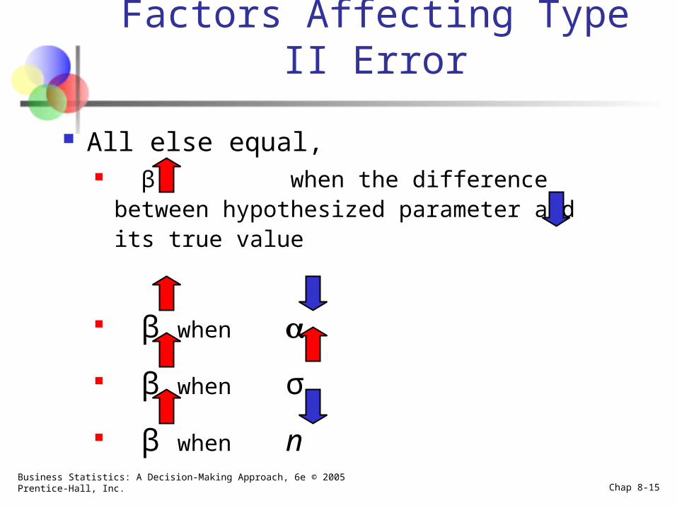
Factors Affecting Type II Error
All else equal, β when the difference between
hypothesized parameter and its true value
β when
β when σ
β when n
Business Statistics: A Decision-Making Approach, 6e © 2005 Prentice-Hall, Inc. Chap 8-16
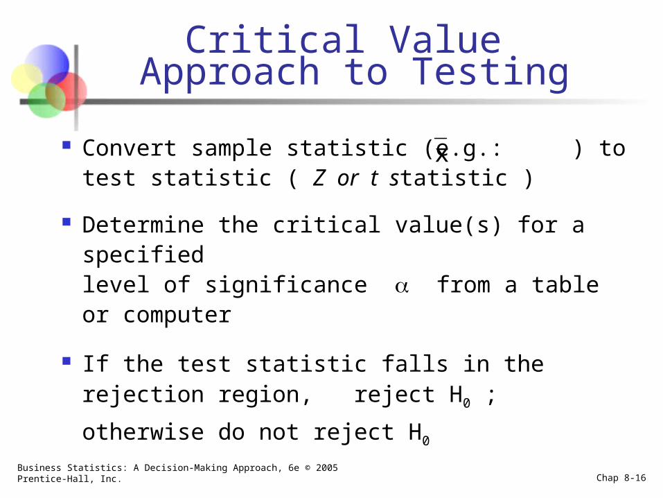
Critical Value Approach to Testing
Convert sample statistic (e.g.: ) to test statistic ( Z or t statistic )
Determine the critical value(s) for a specifiedlevel of significance from a table or computer
If the test statistic falls in the rejection region,
reject H0 ; otherwise do not reject H0
x
Business Statistics: A Decision-Making Approach, 6e © 2005 Prentice-Hall, Inc. Chap 8-17
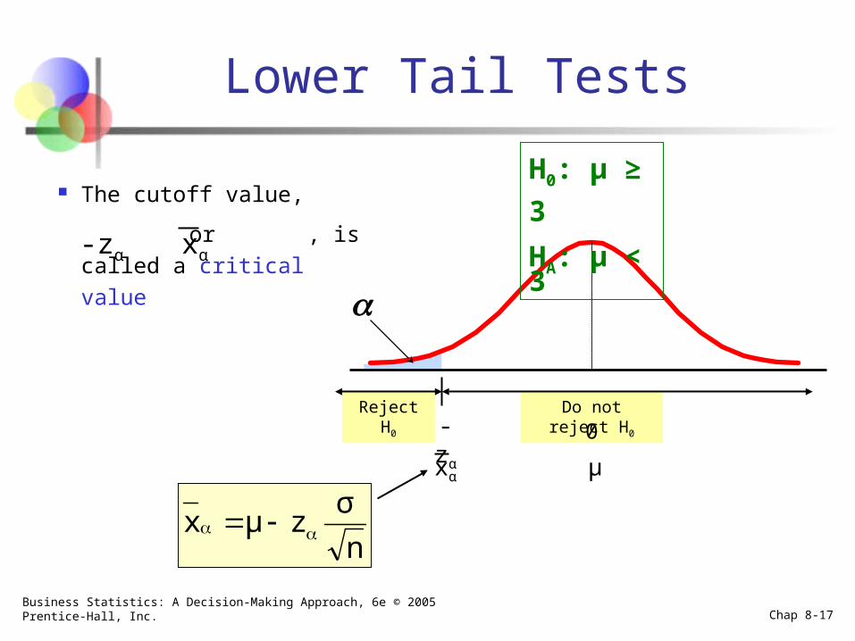
Reject H0 Do not reject H0
The cutoff value,
or , is called a
critical value
Lower Tail Tests
-zα
xα
-zα xα
0
μ
H0: μ ≥ 3
HA: μ < 3
n
σzμx
Business Statistics: A Decision-Making Approach, 6e © 2005 Prentice-Hall, Inc. Chap 8-18
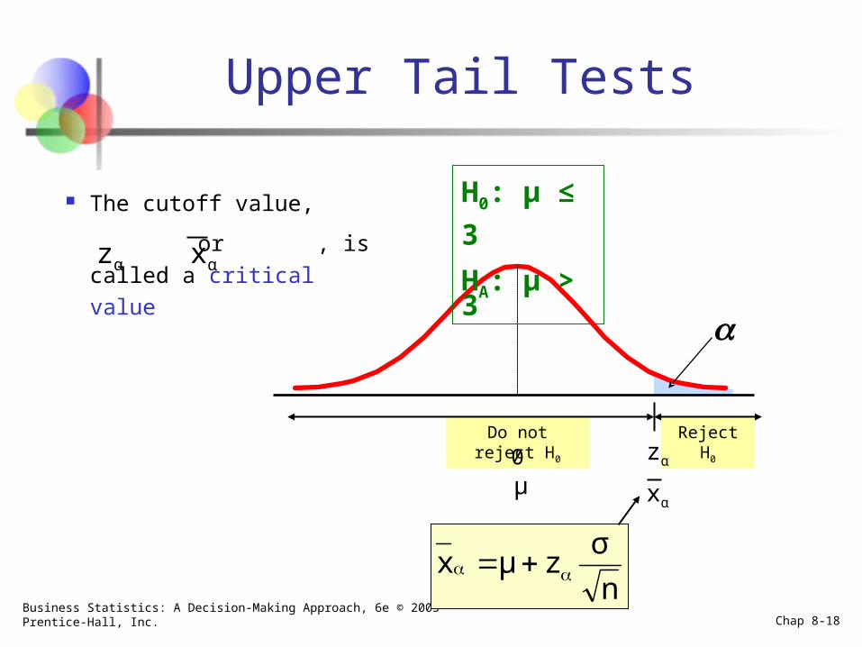
Reject H0Do not reject H0
The cutoff value,
or , is called a
critical value
Upper Tail Tests
zα
xα
zα xα
0μ
H0: μ ≤ 3
HA: μ > 3
n
σzμx
Business Statistics: A Decision-Making Approach, 6e © 2005 Prentice-Hall, Inc. Chap 8-19
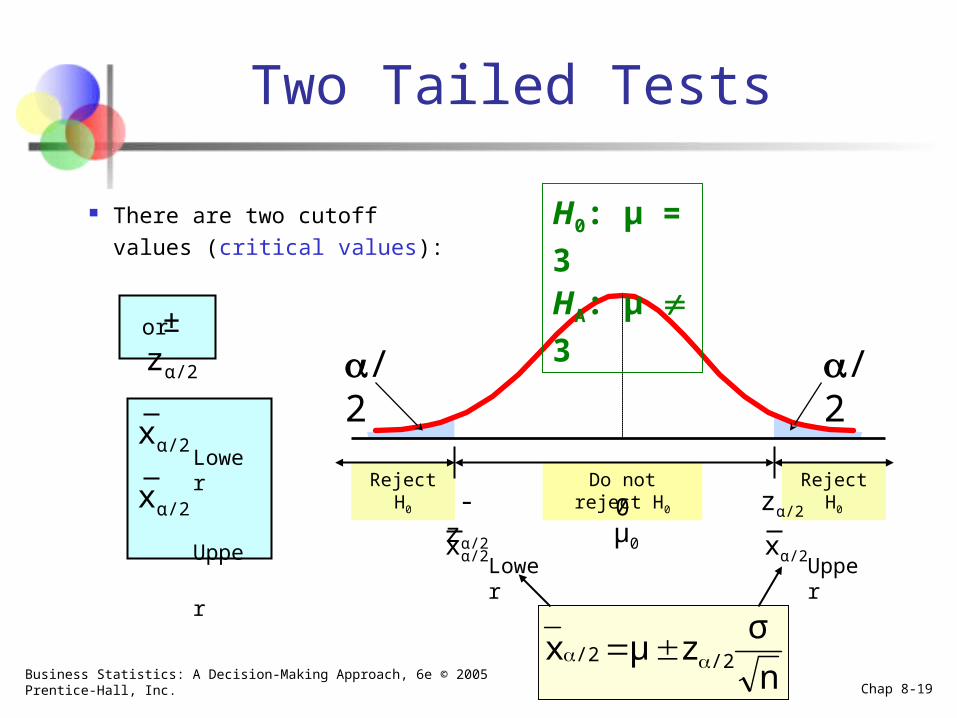
Do not reject H0 Reject H0Reject H0
There are two cutoff values
(critical values):
or
Two Tailed Tests
/2
-zα/2
xα/2
± zα/2
xα/2
0μ0
H0: μ = 3
HA: μ
3
zα/2
xα/2
n
σzμx /2/2
Lower
Upperxα/2
Lower Upper
/2
Business Statistics: A Decision-Making Approach, 6e © 2005 Prentice-Hall, Inc. Chap 8-20
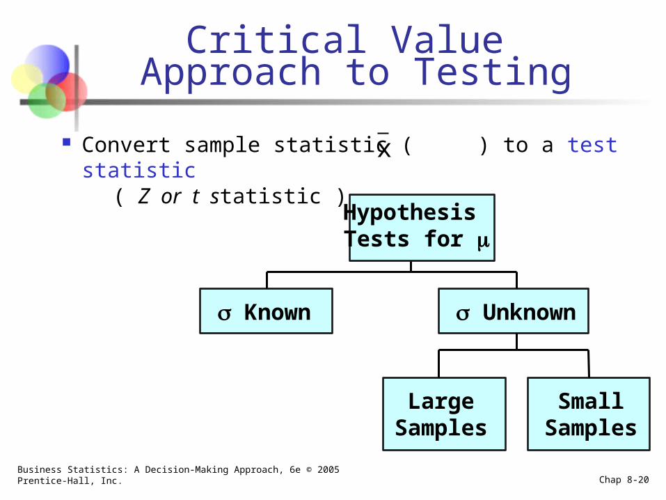
Critical Value Approach to Testing
Convert sample statistic ( ) to a test statistic ( Z or t statistic )
x
Known
Large Samples
Unknown
Hypothesis Tests for
Small Samples
Business Statistics: A Decision-Making Approach, 6e © 2005 Prentice-Hall, Inc. Chap 8-21
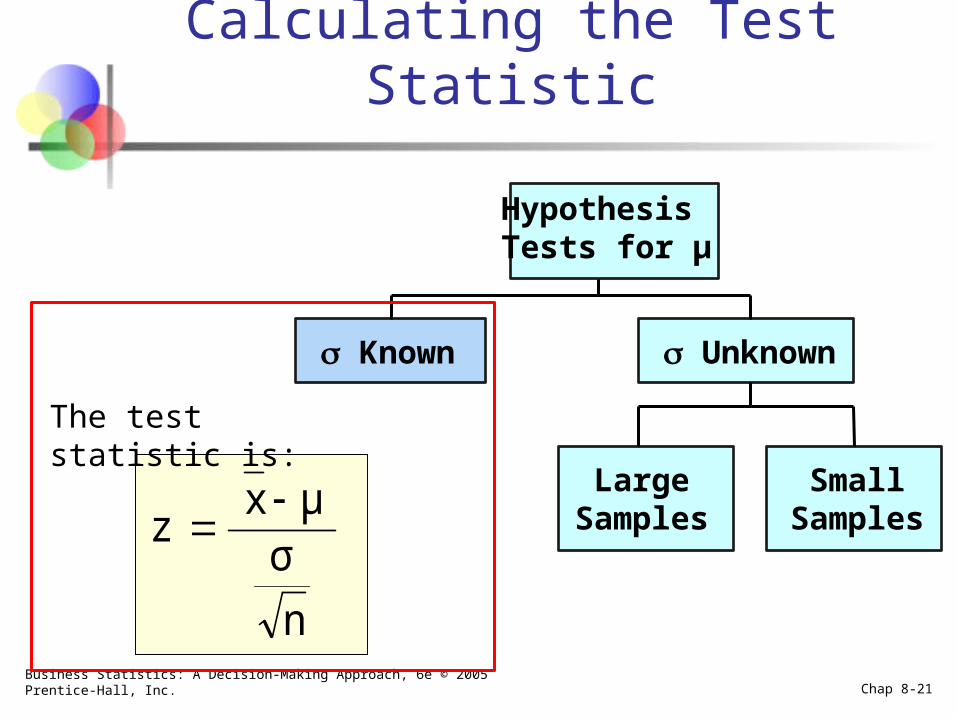
Known
Large Samples
Unknown
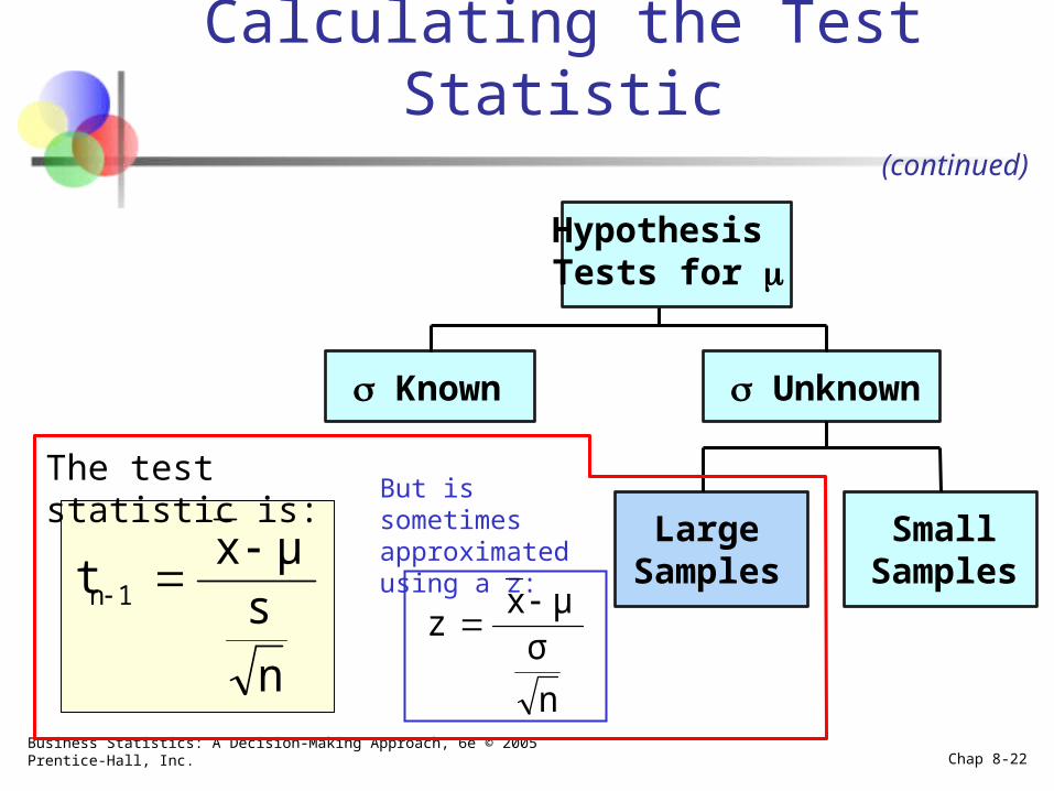
Hypothesis Tests for μ
Small Samples
The test statistic is:
Calculating the Test Statistic
n
σμx
z
Business Statistics: A Decision-Making Approach, 6e © 2005 Prentice-Hall, Inc. Chap 8-22
Known
Large Samples
Unknown
Hypothesis Tests for
Small Samples
The test statistic is:
Calculating the Test Statistic
n
sμx
t 1n
But is sometimes approximated using a z:
n
σμx
z
(continued)
Business Statistics: A Decision-Making Approach, 6e © 2005 Prentice-Hall, Inc. Chap 8-23
Known
Large Samples
Unknown
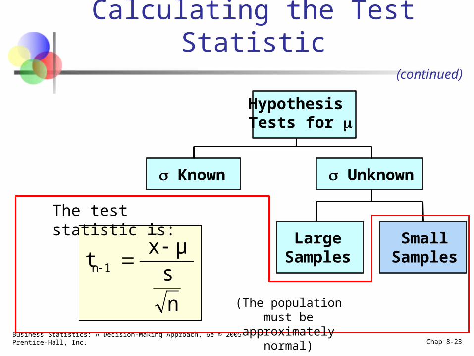
Hypothesis Tests for
Small Samples
The test statistic is:
Calculating the Test Statistic
n
sμx
t 1n
(The population must be approximately normal)
(continued)
Business Statistics: A Decision-Making Approach, 6e © 2005 Prentice-Hall, Inc. Chap 8-24
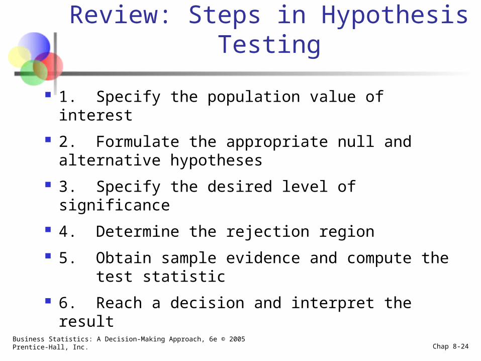
Review: Steps in Hypothesis Testing
1. Specify the population value of interest
2. Formulate the appropriate null and alternative hypotheses
3. Specify the desired level of significance
4. Determine the rejection region
5. Obtain sample evidence and compute the test statistic
6. Reach a decision and interpret the result
Business Statistics: A Decision-Making Approach, 6e © 2005 Prentice-Hall, Inc. Chap 8-25
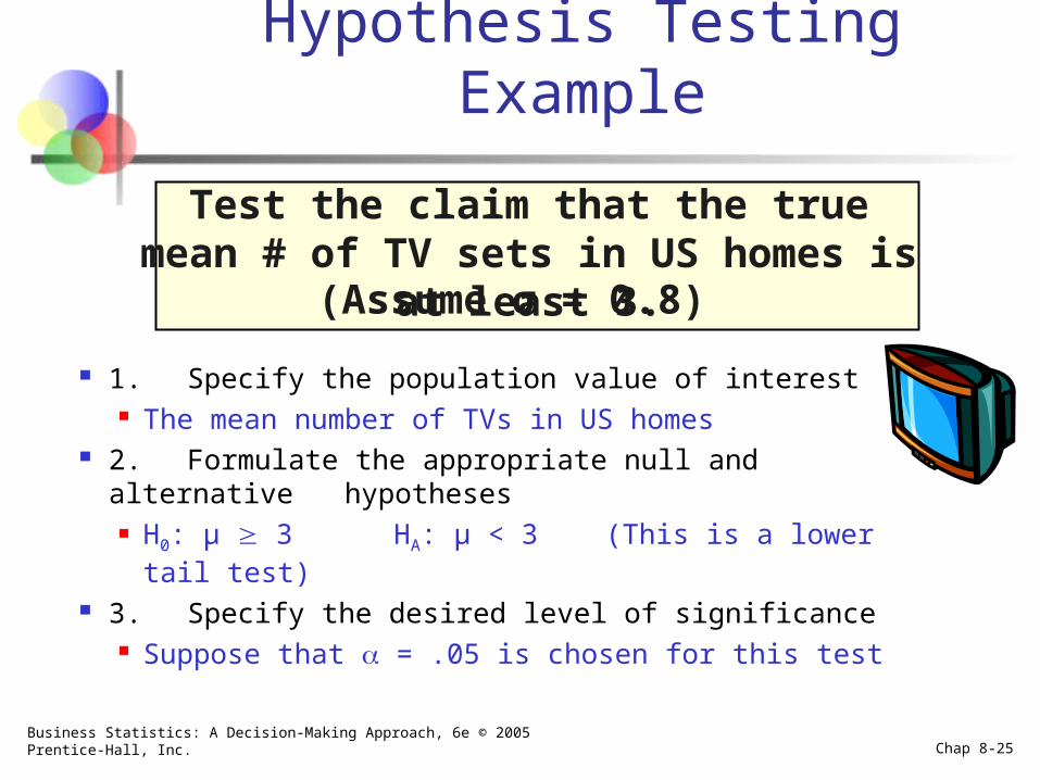
Hypothesis Testing Example
Test the claim that the true mean # of TV sets in US homes is at least 3.
(Assume σ = 0.8)
1. Specify the population value of interest The mean number of TVs in US homes
2. Formulate the appropriate null and alternative hypotheses H0: μ 3 HA: μ < 3 (This is a lower tail test)
3. Specify the desired level of significance Suppose that = .05 is chosen for this test
Business Statistics: A Decision-Making Approach, 6e © 2005 Prentice-Hall, Inc. Chap 8-26
Reject H0 Do not reject H0
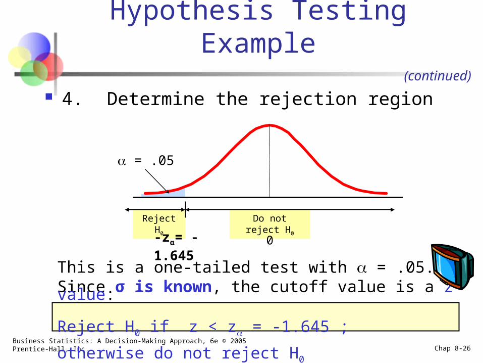
4. Determine the rejection region
= .05
-zα= -1.645 0
This is a one-tailed test with = .05. Since σ is known, the cutoff value is a z value:
Reject H0 if z < z = -1.645 ; otherwise do not reject H0
Hypothesis Testing Example(continued)
Business Statistics: A Decision-Making Approach, 6e © 2005 Prentice-Hall, Inc. Chap 8-27
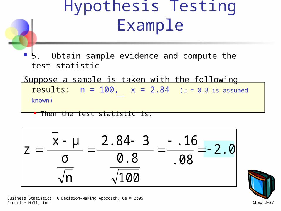
5. Obtain sample evidence and compute the test statistic
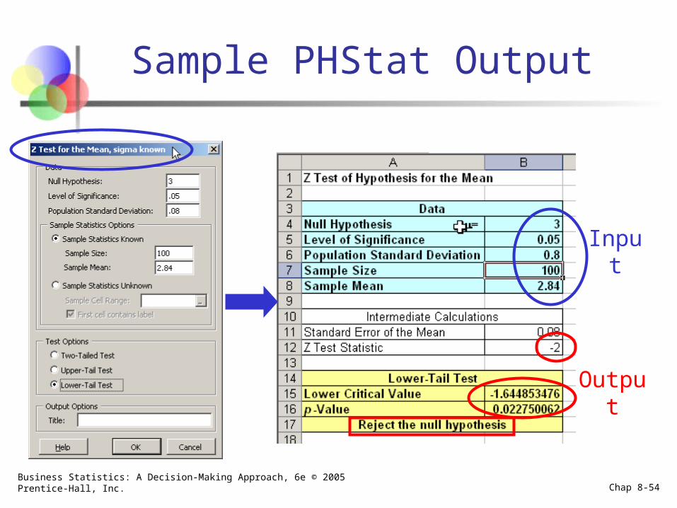
Suppose a sample is taken with the following results: n = 100, x = 2.84 ( = 0.8 is assumed known)
Then the test statistic is:
2.0.08
.16
100
0.832.84
n
σμx
z
Hypothesis Testing Example
Business Statistics: A Decision-Making Approach, 6e © 2005 Prentice-Hall, Inc. Chap 8-28
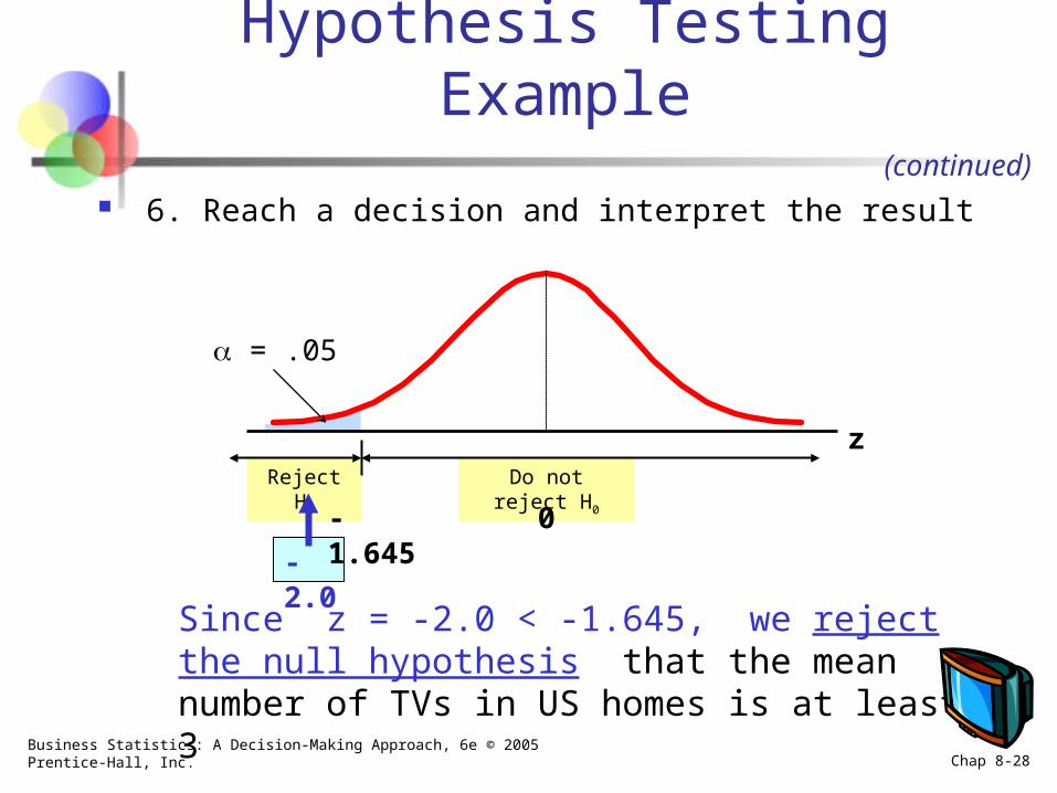
Reject H0 Do not reject H0
= .05
-1.645 0
6. Reach a decision and interpret the result
-2.0
Since z = -2.0 < -1.645, we reject the null hypothesis that the mean number of TVs in US homes is at least 3
Hypothesis Testing Example(continued)
z
Business Statistics: A Decision-Making Approach, 6e © 2005 Prentice-Hall, Inc. Chap 8-29
Reject H0
= .05
2.8684
Do not reject H0
3
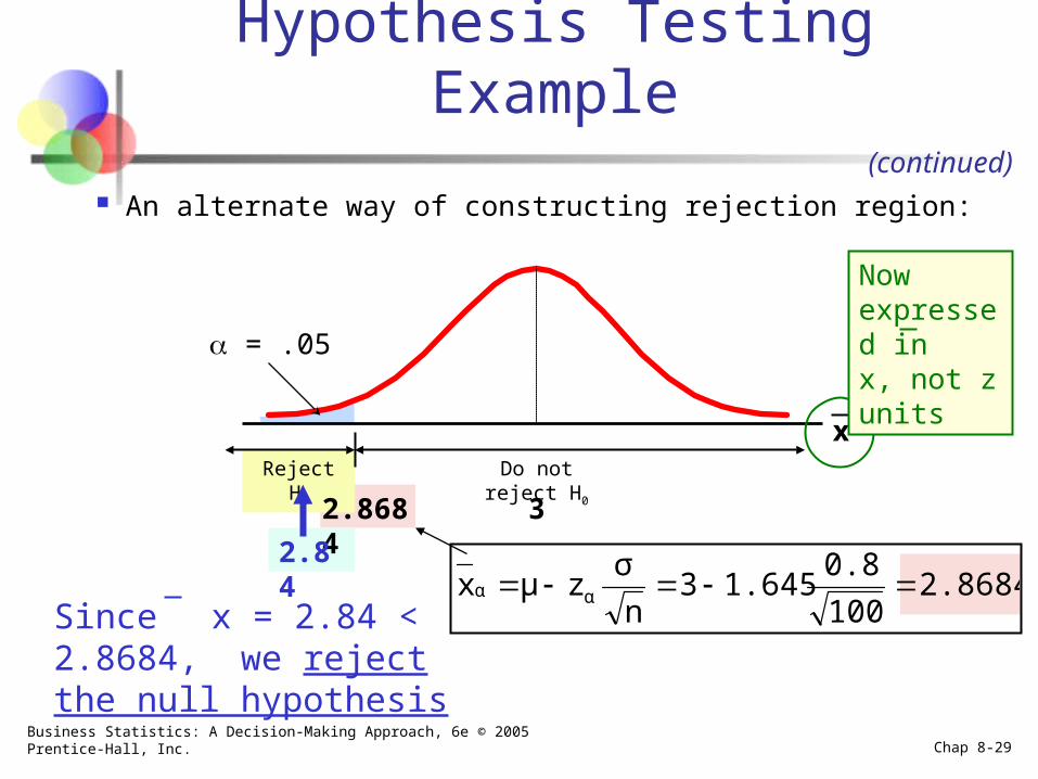
An alternate way of constructing rejection region:
2.84
Since x = 2.84 < 2.8684, we reject the null hypothesis
Hypothesis Testing Example(continued)
x
Now expressed in x, not z units
2.8684100
0.81.6453
n
σzμx αα
Business Statistics: A Decision-Making Approach, 6e © 2005 Prentice-Hall, Inc. Chap 8-30
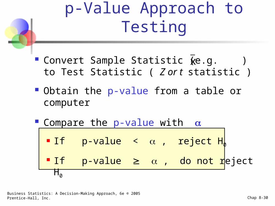
p-Value Approach to Testing
Convert Sample Statistic (e.g. ) to Test Statistic ( Z or t statistic )
Obtain the p-value from a table or computer
Compare the p-value with
If p-value < , reject H0
If p-value , do not reject H0
x
Business Statistics: A Decision-Making Approach, 6e © 2005 Prentice-Hall, Inc. Chap 8-31
p-Value Approach to Testing
p-value: Probability of obtaining a test statistic more extreme ( ≤ or ) than the observed sample value given H0 is
true
Also called observed level of significance
Smallest value of for which H0 can be
rejected
(continued)
Business Statistics: A Decision-Making Approach, 6e © 2005 Prentice-Hall, Inc. Chap 8-32
p-value =.0228
= .05
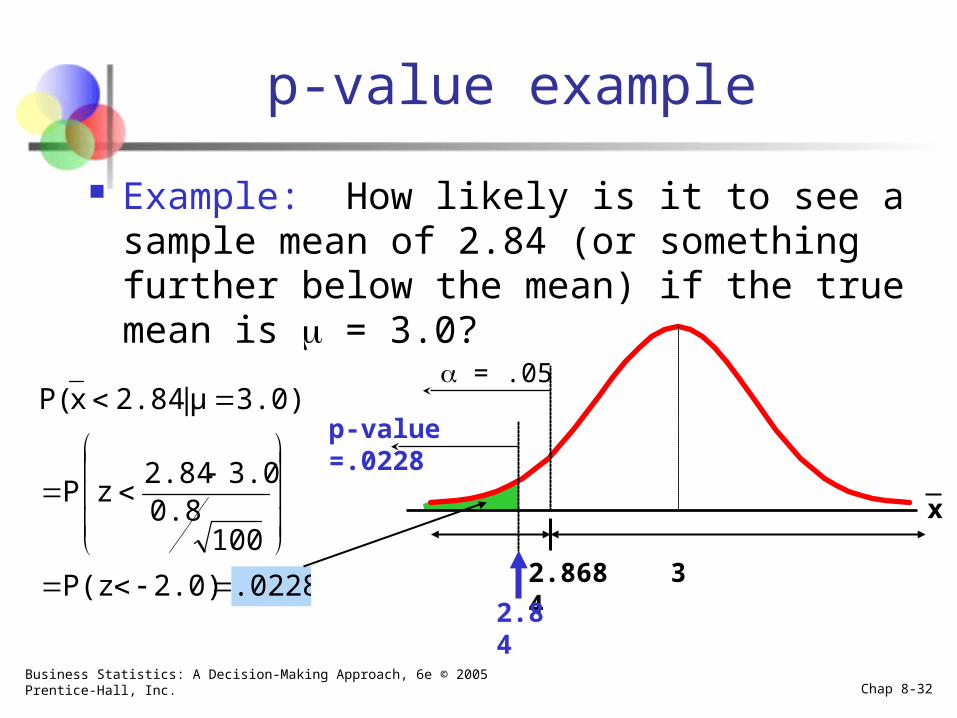
p-value example
Example: How likely is it to see a sample mean of 2.84 (or something further below the mean) if the true mean is = 3.0?
2.8684 3
2.84
x
.02282.0)P(z
1000.8
3.02.84zP
3.0)μ|2.84xP(
Business Statistics: A Decision-Making Approach, 6e © 2005 Prentice-Hall, Inc. Chap 8-33
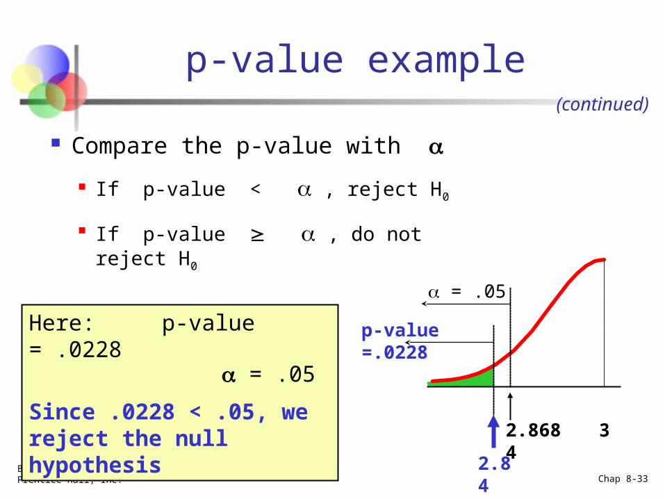
Compare the p-value with
If p-value < , reject H0
If p-value , do not reject H0
Here: p-value = .0228 = .05
Since .0228 < .05, we reject the null hypothesis
(continued)
p-value example
p-value =.0228
= .05
2.8684 3
2.84
Business Statistics: A Decision-Making Approach, 6e © 2005 Prentice-Hall, Inc. Chap 8-34
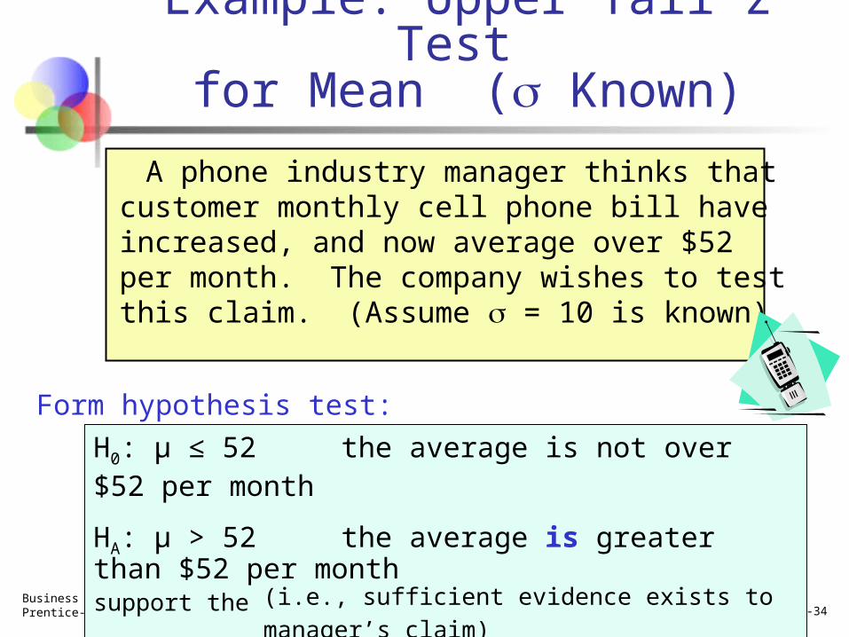
Example: Upper Tail z Test for Mean ( Known)
A phone industry manager thinks that customer monthly cell phone bill have increased, and now average over $52 per month. The company wishes to test this claim. (Assume = 10 is known)
H0: μ ≤ 52 the average is not over $52 per month
HA: μ > 52 the average is greater than $52 per month(i.e., sufficient evidence exists to support the manager’s claim)
Form hypothesis test:
Business Statistics: A Decision-Making Approach, 6e © 2005 Prentice-Hall, Inc. Chap 8-35
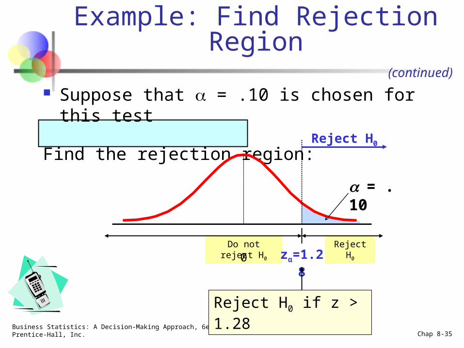
Reject H0Do not reject H0
Suppose that = .10 is chosen for this test
Find the rejection region:
= .10
zα=1.280
Reject H0
Reject H0 if z > 1.28
Example: Find Rejection Region
(continued)
Business Statistics: A Decision-Making Approach, 6e © 2005 Prentice-Hall, Inc. Chap 8-36
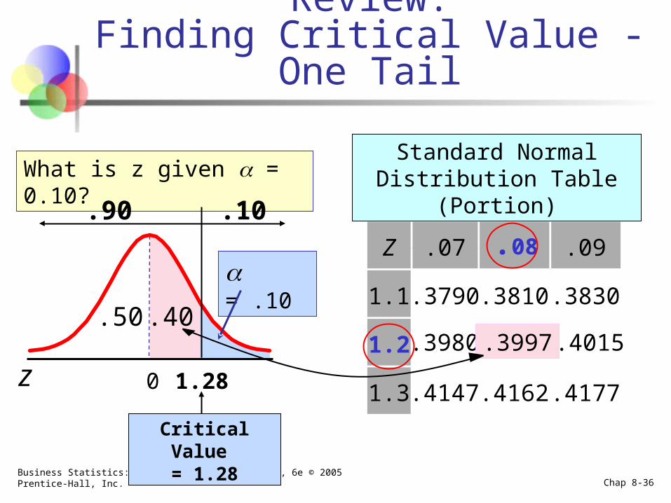
Review:Finding Critical Value - One
Tail
Z .07 .09
1.1 .3790 .3810 .3830
1.2 .3980 .4015
1.3 .4147 .4162 .4177z 0 1.28
.08
Standard Normal Distribution Table (Portion)What is z given =
0.10?
= .10
Critical Value = 1.28
.90
.3997
.10
.40.50
Business Statistics: A Decision-Making Approach, 6e © 2005 Prentice-Hall, Inc. Chap 8-37
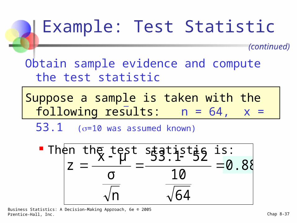
Obtain sample evidence and compute the test statistic
Suppose a sample is taken with the following results: n = 64, x = 53.1 (=10 was assumed known)
Then the test statistic is:
0.88
64
105253.1
n
σμx
z
Example: Test Statistic(continued)
Business Statistics: A Decision-Making Approach, 6e © 2005 Prentice-Hall, Inc. Chap 8-38
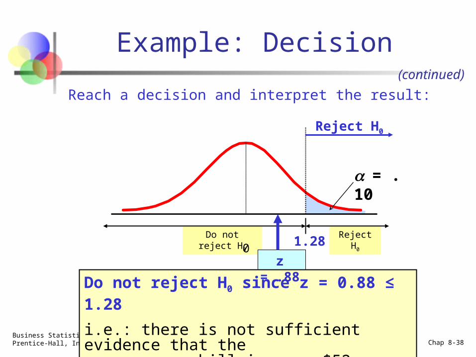
Reject H0Do not reject H0
Example: Decision
= .10
1.280
Reject H0
Do not reject H0 since z = 0.88 ≤ 1.28
i.e.: there is not sufficient evidence that the mean bill is over $52
z = .88
Reach a decision and interpret the result:(continued)
Business Statistics: A Decision-Making Approach, 6e © 2005 Prentice-Hall, Inc. Chap 8-39
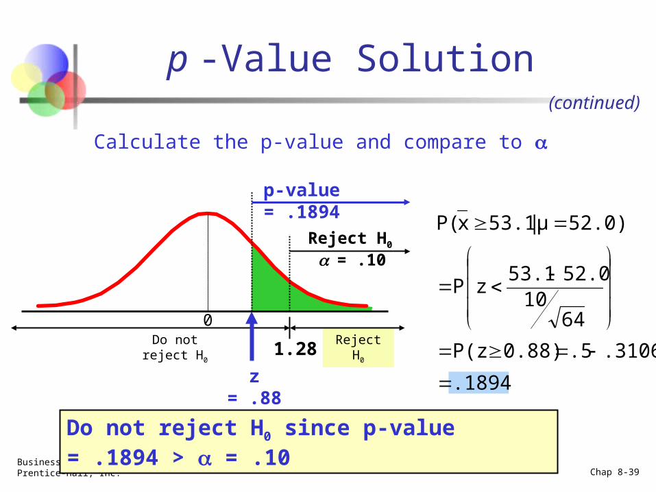
Reject H0
= .10
Do not reject H0 1.28
0
Reject H0
z = .88
Calculate the p-value and compare to
(continued)
.1894
.3106.50.88)P(z
6410
52.053.1zP
52.0)μ|53.1xP(
p-value = .1894
p -Value Solution
Do not reject H0 since p-value = .1894 > = .10
Business Statistics: A Decision-Making Approach, 6e © 2005 Prentice-Hall, Inc. Chap 8-40
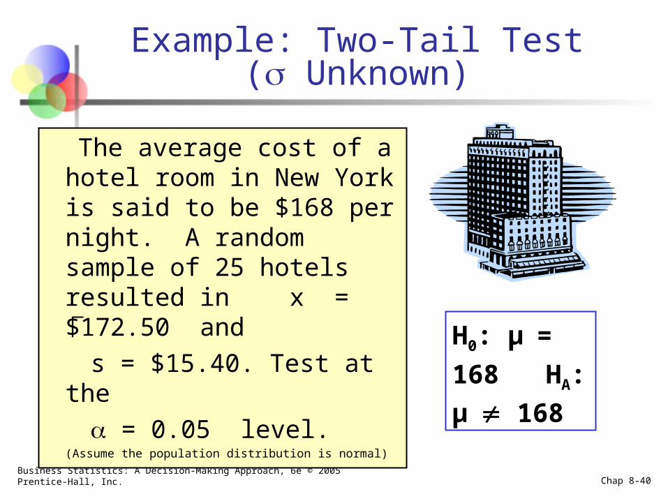
Example: Two-Tail Test( Unknown)
The average cost of a hotel room in New York is said to be $168 per night. A random sample of 25 hotels resulted in x = $172.50 and
s = $15.40. Test at the
= 0.05 level.(Assume the population distribution is normal)
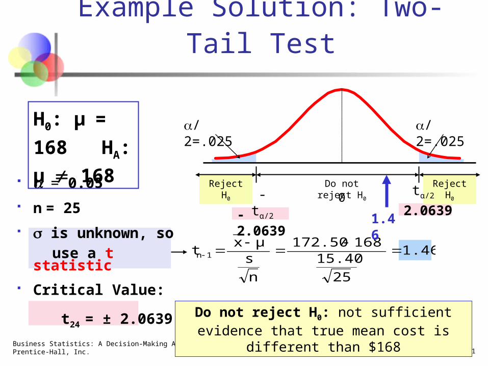
H0: μ= 168
HA: μ
168
Business Statistics: A Decision-Making Approach, 6e © 2005 Prentice-Hall, Inc. Chap 8-41
= 0.05
n = 25
is unknown, so use a t statistic
Critical Value:
t24 = ± 2.0639
Example Solution: Two-Tail Test
Do not reject H0: not sufficient evidence that true mean cost is different than $168
Reject H0Reject H0
/2=.025
-tα/2
Do not reject H0
0 tα/2
/2=.025
-2.0639 2.0639
1.46
25
15.40168172.50
n
sμx
t 1n
1.46
H0: μ= 168
HA: μ
168
Business Statistics: A Decision-Making Approach, 6e © 2005 Prentice-Hall, Inc. Chap 8-42
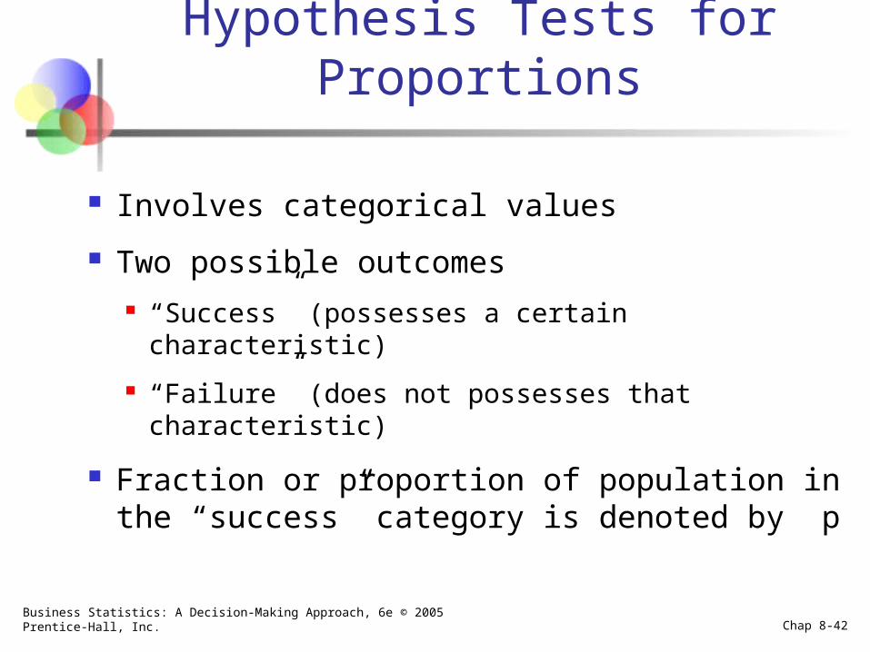
Hypothesis Tests for Proportions
Involves categorical values
Two possible outcomes “Success” (possesses a certain characteristic)
“Failure” (does not possesses that characteristic)
Fraction or proportion of population in the “success” category is denoted by p
Business Statistics: A Decision-Making Approach, 6e © 2005 Prentice-Hall, Inc. Chap 8-43
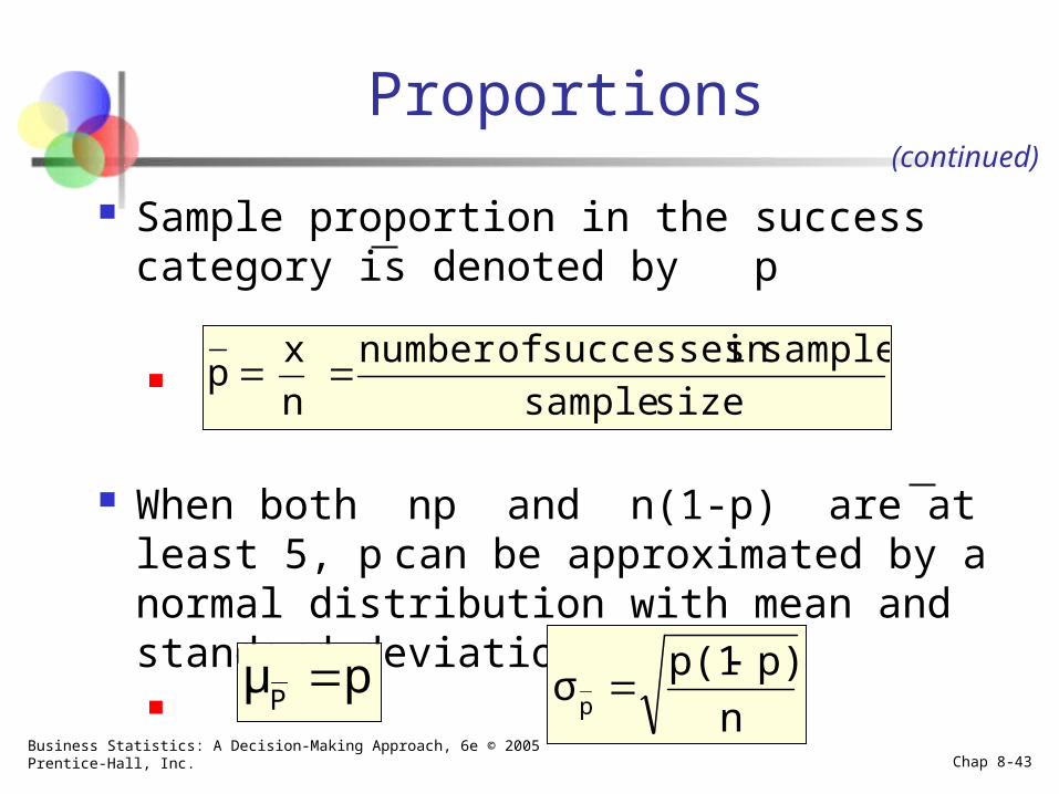
Proportions
Sample proportion in the success category is denoted by p
When both np and n(1-p) are at least 5, p can be approximated by a normal distribution with mean and standard deviation
(continued)
sizesample
sampleinsuccessesofnumber
n
xp
pμP
n
p)p(1σ
p
Business Statistics: A Decision-Making Approach, 6e © 2005 Prentice-Hall, Inc. Chap 8-44
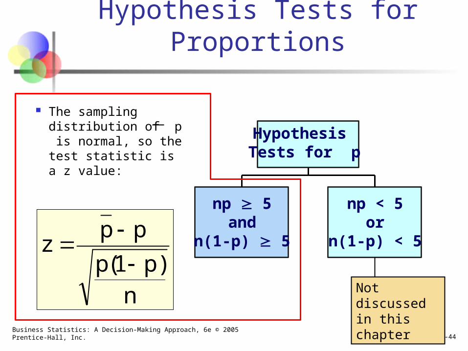
The sampling distribution of p is normal, so the test statistic is a z value:
Hypothesis Tests for Proportions
n)p(p
ppz
1
np 5and
n(1-p) 5
Hypothesis Tests for p
np < 5or
n(1-p) < 5
Not discussed in this chapter
Business Statistics: A Decision-Making Approach, 6e © 2005 Prentice-Hall, Inc. Chap 8-45
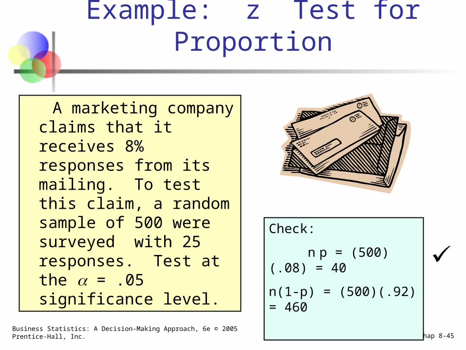
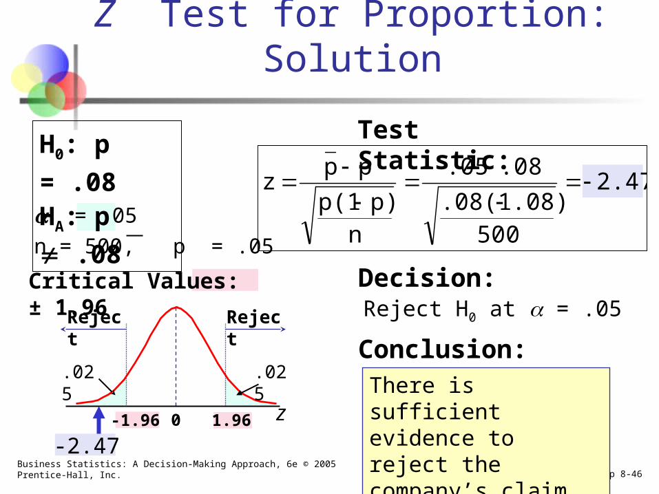
Example: z Test for Proportion
A marketing company claims that it receives 8% responses from its mailing. To test this claim, a random sample of 500 were surveyed with 25 responses. Test at the = .05 significance level.
Check:
n p = (500)(.08) = 40
n(1-p) = (500)(.92) = 460
Business Statistics: A Decision-Making Approach, 6e © 2005 Prentice-Hall, Inc. Chap 8-46
Z Test for Proportion: Solution
= .05
n = 500, p = .05
Reject H0 at = .05
H0: p = .08
HA: p
.08
Critical Values: ± 1.96
Test Statistic:
Decision:
Conclusion:
z0
Reject Reject
.025.025
1.96
-2.47
There is sufficient evidence to reject the company’s claim of 8% response rate.
2.47
500.08).08(1
.08.05
np)p(1
ppz
-1.96
Business Statistics: A Decision-Making Approach, 6e © 2005 Prentice-Hall, Inc. Chap 8-47
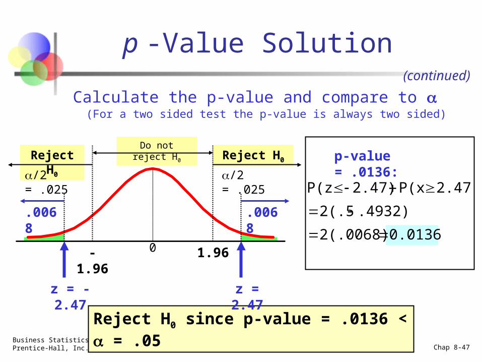
Do not reject H0
Reject H0Reject H0
/2 = .025
1.960
z = -2.47
Calculate the p-value and compare to (For a two sided test the p-value is always two sided)
(continued)
0.01362(.0068)
.4932)2(.5
2.47)P(x2.47)P(z
p-value = .0136:
p -Value Solution
Reject H0 since p-value = .0136 < = .05
z = 2.47
-1.96
/2 = .025
.0068.0068
Business Statistics: A Decision-Making Approach, 6e © 2005 Prentice-Hall, Inc. Chap 8-48
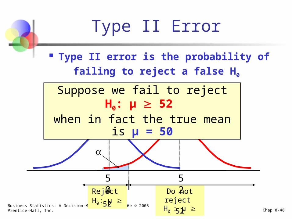
Reject H0: μ 52
Do not reject H0 : μ 52
Type II Error
Type II error is the probability of
failing to reject a false H0
5250
Suppose we fail to reject H0: μ 52 when in fact the true mean is μ = 50
Business Statistics: A Decision-Making Approach, 6e © 2005 Prentice-Hall, Inc. Chap 8-49
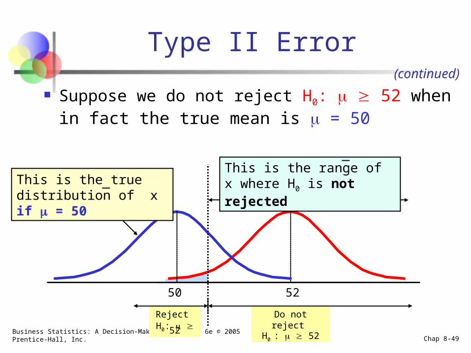
Reject H0: 52
Do not reject H0 : 52
Type II Error
Suppose we do not reject H0: 52 when in fact the true mean is = 50
5250
This is the true distribution of x if = 50
This is the range of x where H0 is not rejected
(continued)
Business Statistics: A Decision-Making Approach, 6e © 2005 Prentice-Hall, Inc. Chap 8-50
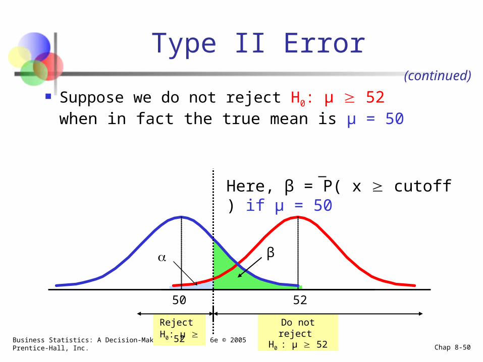
Reject H0: μ 52
Do not reject H0 : μ 52
Type II Error
Suppose we do not reject H0: μ 52 when in fact the true mean is μ = 50
5250
β
Here, β = P( x cutoff ) if μ = 50
(continued)
Business Statistics: A Decision-Making Approach, 6e © 2005 Prentice-Hall, Inc. Chap 8-51
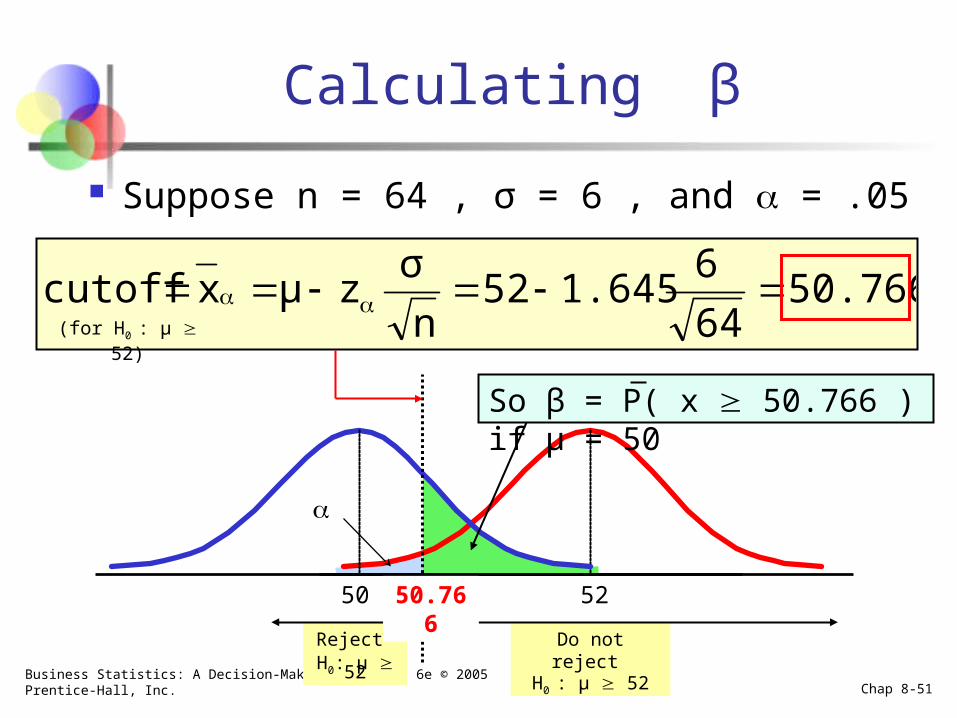
Reject H0: μ 52
Do not reject H0 : μ 52
Suppose n = 64 , σ = 6 , and = .05
5250
So β = P( x 50.766 ) if μ = 50
Calculating β
50.76664
61.64552
n
σzμxcutoff
(for H0 : μ 52)
50.766
Business Statistics: A Decision-Making Approach, 6e © 2005 Prentice-Hall, Inc. Chap 8-52
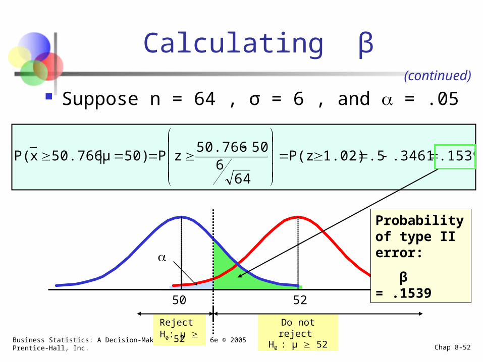
Reject H0: μ 52
Do not reject H0 : μ 52
.1539.3461.51.02)P(z
646
5050.766zP50)μ|50.766xP(
Suppose n = 64 , σ = 6 , and = .05
5250
Calculating β(continued)
Probability of type II error:
β = .1539
Business Statistics: A Decision-Making Approach, 6e © 2005 Prentice-Hall, Inc. Chap 8-53
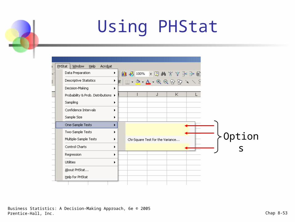
Using PHStat
Options
Business Statistics: A Decision-Making Approach, 6e © 2005 Prentice-Hall, Inc. Chap 8-54
Sample PHStat Output
Input
Output
Business Statistics: A Decision-Making Approach, 6e © 2005 Prentice-Hall, Inc. Chap 8-55
Chapter Summary
Addressed hypothesis testing methodology
Performed z Test for the mean (σ known)
Discussed p–value approach to hypothesis testing
Performed one-tail and two-tail tests . . .
Business Statistics: A Decision-Making Approach, 6e © 2005 Prentice-Hall, Inc. Chap 8-56
Chapter Summary
Performed t test for the mean (σ unknown)
Performed z test for the proportion
Discussed type II error and computed its probability
(continued)


![[PPT]Business Statistics: A Decision-Making Approach, 7th …ychoi2/MGMT_BA 301/Ch05/groebner8_ch05.ppt · Web viewTitle Business Statistics: A Decision-Making Approach, 7th edition](https://img.pdfslide.us/doc/110x75/5af95dc67f8b9a32348c4cb4/pptbusiness-statistics-a-decision-making-approach-7th-ychoi2mgmtba-301ch05groebner8ch05pptweb.jpg)